Numerical and experimental analysis of local flow

Numerical and experimental analysis of local flow phenomena in laminarTaylor flow in a square mini-channelC. J. Falconi, C. Lehrenfeld, H. Marschall, C. Meyer, R. Abiev, D. Bothe, A. Reusken, M. Schlüter,and M. Wörner Citation: Physics of Fluids 28, 012109 (2016); doi: 10.1063/1.4939498 View online: http://dx.doi.org/10.1063/1.4939498 View Table of Contents: http://scitation.aip.org/content/aip/journal/pof2/28/1?ver=pdfcov Published by the AIP Publishing Articles you may be interested in Inertia-driven particle migration and mixing in a wall-bounded laminar suspension flow Phys. Fluids 27, 123304 (2015); 10.1063/1.4936402 Experimental and numerical study of buoyancy-driven single bubble dynamics in a vertical Hele-Shaw cell Phys. Fluids 26, 123303 (2014); 10.1063/1.4903488 Migration of finite sized particles in a laminar square channel flow from low to high Reynoldsnumbers Phys. Fluids 26, 123301 (2014); 10.1063/1.4902952 The effect of neutrally buoyant finite-size particles on channel flows in the laminar-turbulenttransition regime Phys. Fluids 25, 123304 (2013); 10.1063/1.4848856 Analysis of non-spherical particle transport in complex internal shear flows Phys. Fluids 25, 091904 (2013); 10.1063/1.4821812

This article is copyrighted as indicated in the article. Reuse of AIP content is subject to the terms at: http://scitation.aip.org/termsconditions. Downloaded

to IP: 134.130.161.251 On: Mon, 18 Jan 2016 11:24:37

http://scitation.aip.org/content/aip/journal/pof2?ver=pdfcov

http://oasc12039.247realmedia.com/RealMedia/ads/click_lx.ads/www.aip.org/pt/adcenter/pdfcover_test/L-37/614767649/x01/AIP-PT/PoF_ArticleDL_0116/AIP-APL_Photonics_Launch_1640x440_general_PDF_ad.jpg/434f71374e315a556e61414141774c75?x

http://scitation.aip.org/search?value1=C.+J.+Falconi&option1=author

http://scitation.aip.org/search?value1=C.+Lehrenfeld&option1=author

http://scitation.aip.org/search?value1=H.+Marschall&option1=author

http://scitation.aip.org/search?value1=C.+Meyer&option1=author

http://scitation.aip.org/search?value1=R.+Abiev&option1=author

http://scitation.aip.org/search?value1=D.+Bothe&option1=author

http://scitation.aip.org/search?value1=A.+Reusken&option1=author

http://scitation.aip.org/search?value1=M.+Schlter&option1=author

http://scitation.aip.org/search?value1=M.+Wrner&option1=author

http://scitation.aip.org/content/aip/journal/pof2?ver=pdfcov

http://dx.doi.org/10.1063/1.4939498

http://scitation.aip.org/content/aip/journal/pof2/28/1?ver=pdfcov

http://scitation.aip.org/content/aip?ver=pdfcov

http://scitation.aip.org/content/aip/journal/pof2/27/12/10.1063/1.4936402?ver=pdfcov








PHYSICS OF FLUIDS 28, 012109 (2016)

Numerical and experimental analysis of local flowphenomena in laminar Taylor flow in a squaremini-channel

C. J. Falconi,1,a) C. Lehrenfeld,2,b) H. Marschall,3 C. Meyer,4 R. Abiev,5D. Bothe,3 A. Reusken,2 M. Schlüter,4 and M. Wörner1,c)1Institute of Catalysis Research and Technology, Karlsruhe Institute of Technology,Karlsruhe, Germany2Institut für Geometrie und Praktische Mathematik, RWTH Aachen, Aachen, Germany3Center of Smart Interfaces, Technical University Darmstadt, Darmstadt, Germany4Institute of Multiphase Flows, Technical University Hamburg-Harburg, Hamburg, Germany5St. Petersburg State Institute of Technology, St. Petersburg, Russia

(Received 12 March 2015; accepted 21 December 2015; published online 12 January 2016)

The vertically upward Taylor flow in a small square channel (side length 2 mm) is oneof the guiding measures within the priority program “Transport Processes at FluidicInterfaces” (SPP 1506) of the German Research Foundation (DFG). This paper pres-ents the results of coordinated experiments and three-dimensional numerical simula-tions (with three different academic computer codes) for typical local flow parameters(bubble shape, thickness of the liquid film, and velocity profiles) in different cuttingplanes (lateral and diagonal) for a specific co-current Taylor flow. For most quantities,the differences between the three simulation results and also between the numericaland experimental results are below a few percent. The experimental and computationalresults consistently show interesting three-dimensional flow effects in the rear partof the liquid film. There, a local back flow of liquid occurs in the fixed frame ofreference which leads to a temporary reversal of the direction of the wall shear stressduring the passage of a Taylor bubble. Notably, the axial positions of the region withlocal backflow and those of the minimum vertical velocity differ in the lateral andthe diagonal liquid films. By a thorough analysis of the fully resolved simulationresults, this previously unknown phenomenon is explained in detail and, moreover,approximate criteria for its occurrence in practical applications are given. It is thedifferent magnitude of the velocity in the lateral film and in the corner region whichleads to azimuthal pressure differences in the lateral and diagonal liquid films andcauses a slight deviation of the bubble from the rotational symmetry. This deviationis opposite in the front and rear parts of the bubble and has the mentioned significanteffects on the local flow field in the rear part of the liquid film. C 2016 AIP PublishingLLC. [http://dx.doi.org/10.1063/1.4939498]

I. INTRODUCTION

For interface resolving simulation of two-phase flows, various numerical methods are avail-able.1–4 These encompass nowadays well-established methods such as the volume-of-fluid method,the level-set method, the front-tracking method, as well as emerging methods such as the lattice Boltz-mann method. Among other areas of fundamental research, these methods are attractive to studytwo-phase flows in microfluidics and micro-process engineering numerically. In such applications,the gas/liquid or liquid/liquid flows are predominantly laminar and the number of bubbles or drops issufficiently small to be computationally manageable, see, e.g., the work of Wörner5 for a recent review.

a)Present address: Automotive Simulation Center Stuttgart e.V., Stuttgart, Germany.b)Present address: Institute for Computational and Applied Mathematics, University Münster, Münster, Germany.c)Author to whom correspondence should be addressed. Electronic mail: [email protected]

1070-6631/2016/28(1)/012109/23/$30.00 28, 012109-1 ©2016 AIP Publishing LLC


to IP: 134.130.161.251 On: Mon, 18 Jan 2016 11:24:37

http://dx.doi.org/10.1063/1.4939498

http://dx.doi.org/10.1063/1.4939498

http://dx.doi.org/10.1063/1.4939498

http://dx.doi.org/10.1063/1.4939498

http://dx.doi.org/10.1063/1.4939498

http://dx.doi.org/10.1063/1.4939498

http://dx.doi.org/10.1063/1.4939498

http://dx.doi.org/10.1063/1.4939498

http://dx.doi.org/10.1063/1.4939498

http://dx.doi.org/10.1063/1.4939498

http://dx.doi.org/10.1063/1.4939498

mailto:[email protected]






















http://crossmark.crossref.org/dialog/?doi=10.1063/1.4939498&domain=pdf&date_stamp=2016-01-12

012109-2 Falconi et al. Phys. Fluids 28, 012109 (2016)

An important point for the assessment of the accuracy of these numerical methods and their furtheradvancement towards valuable tools for engineering applications is the absence of local experimentaldata for detailed validation on practical flow problems. Additional difficulties in many technical appli-cations are caused by contaminants which may influence or even dominate the behavior of movinginterfaces.

A prototypical problem for two-phase flows in narrow channels is the Taylor flow. It is sometimesalso referred to as bubble-train flow, segmented flow, or capillary slug flow6 and consists of a regularsequence of elongated gas bubbles which almost fill the entire channel cross section (Dumitrescu-Taylor bubbles7,8) and are separated by liquid slugs. Gas-liquid Taylor flow in narrow channels isof interest in micro-process engineering,9,10 catalytically coated monolith reactors,11 material syn-thesis,12–14 and stimulus of biological cells.15 While many experimental and numerical studies onTaylor bubbles or Taylor flow consider circular channels, square channels are potentially of largertechnological relevance for certain applications, but are less often studied. There is, however, anincreasing interest to investigate bubble train flow and gas-liquid Taylor flow in square or rectangularchannels experimentally16–27 and by three-dimensional numerical simulations.28–37 Recent reviewson gas-liquid Taylor flow are provided by Angeli and Gavriilidis,38 Gupta et al.,39 Sobieszuk et al.,40

and Talimi et al.,41 and the reader is referred to these articles and the references therein for furtherexperimental and numerical studies on this subject.

Within the priority programme “Transport Processes at Fluidic Interfaces” (SPP 1506) of theGerman Research Foundation (DFG), Taylor bubbles and Taylor flow in a circular and squaremini-channel are proposed as physical benchmark problems for interface-resolving simulationmethods.37,42,43 In the work of Marschall et al.,37 a combined experimental and numerical study on asingle Taylor bubble in a square vertical mini-channel is presented. The comparison focused on thenon-axisymmetric bubble shape, where precise profiles were measured in longitudinal cuts in lateraland diagonal directions by synchrotron radiation in conjunction with ultrafast radiographic imaging.27

The influence of different numerical methods for interface resolving simulations and different surfacetension force approximations is investigated and, in general, a very good agreement between the fourconsidered codes and the experimental interface profile is found (especially as concerns the curvatureof the front and rear menisci).37 However, some differences occurred with respect to the minimumthickness of the liquid film which separates the bubble from the channel walls. A drawback of thisstudy is that no experimental data on the local velocity field are available for a comparison.

In the present paper, a similar combined experimental and numerical study as in the work ofMarschall et al.37 is performed but with focus on local features of the velocity field, which is measuredwithin the liquid phase by micro-Particle-Image-Velocimetry (µPIV). Such measurements are stillrare, especially within the liquid film. Meyer et al.44 provide a detailed overview on related experi-mental studies in the literature. In contrast to our previous study,37 which dealt with a single Taylorbubble, Taylor flow is considered in the present paper. The liquid slug length is rather short so that thePoiseuille velocity profile is not fully developed and there is a notable interaction between neighboringTaylor bubbles.

As a first goal of our combined experimental and numerical study, we provide quantitative localvelocity field information, e.g., velocity profiles for one particular Taylor flow. Obtaining quantitativebenchmark results with a single computer code is difficult, since the accuracy of the code must beguaranteed which is hard to achieve for the rather complex Taylor flow in a square channel. Here, wedecided to use three academic in-house codes which differ with respect to the numerical method andcertain aspects concerning the numerical setup (due to code-internal restrictions). For many quantitieslike bubble velocity, bubble length, liquid slug length, local bubble radius, and local axial centerlinevelocity in the liquid slug, the differences between the three simulation results and also between thenumerical and experimental results are below a few percent. We consider these simulations’ results tobe useful quantities for comparison in future fluid dynamic simulations of Taylor flow. Furthermore,the numerical and experimental results reveal some interesting phenomena, namely, a local backflowin the rear part of the liquid film. Such a local backflow in a fixed frame of reference was already foundin the numerical simulations of Quan45 who studied the effects of a co-current upward and downwardflow on a single Taylor bubble in a round capillary with a diameter of 3.2 cm. His results show thatthe velocity profile in the liquid film is almost independent of the mean velocity of the co-current


to IP: 134.130.161.251 On: Mon, 18 Jan 2016 11:24:37


flow. Interestingly, the present results for a square channel show that the axial locations of this localbackflow region differ in the lateral film and in the corner film. To the best of our knowledge, thisbehavior has not been reported in the literature so far.

As a second goal, it is demonstrated how the present integrated experimental and computationalstudy can provide a detailed insight and understanding of this local flow phenomenon. The role of theexperiment was to demonstrate that this feature, which is observed in computational fluid dynamics(CFD) simulations under idealized conditions (clean interfaces), is not a numerical artifact but isobserved in real Taylor flow. The role of the computations was to provide fully resolved informationon the bubble shape, the velocity field, and the pressure field in the entire Taylor flow unit cell (whichconsists of one Taylor bubble and one liquid slug). Only these data — which cannot be obtained in theircompleteness nowadays by the even most advanced experimental techniques — provide the informa-tion to understand in detail the underlying hydrodynamics and to derive criteria for the occurrence ofthis phenomenon in practical flow systems.

The paper is organized as follows. Section II gives an overview on the experimental setup andmeasurement techniques. Section III presents the numerical counterpart. In Section IV, the experi-mental and numerical results are compared. In Section V, a physical explanation for the local backflowin the liquid film is given and the conditions under which it may occur are discussed. The paper closeswith conclusions in Section VI.

II. EXPERIMENTS

The present experiment considers a co-current upward Taylor flow in a square vertical mini-channel with cross section 2.076 mm × 2.076 mm and corresponds to scenario “TFSC Small Slug”in the work of Meyer et al.44 The liquid phase is a water/glycerol mixture and the gas phase is air.Special care has been given to the generation of an almost ideal Taylor flow, where bubbles of identicalvolume and shape move with identical velocity and are separated from each other by liquid slugs ofidentical length. By a special injection valve combined with an extraordinary compensation pipe, itwas possible to produce a Taylor flow where the standard deviations in bubble length and slug lengthare below 3% and that of the bubble velocity is below 2%.44

For accurate µPIV measurements of the velocity in the liquid film, the following procedure isadopted. To achieve precise optical access without refraction caused by curved interfaces, refractiveindex matching (RIM) is used. The glass capillary is surrounded by another (larger) capillary filledwith a mixture of Dimethylsulfoxide (DMSO) and distilled water (volume concentration of DMSO inthe DMSO/water mixture is 95%), see Fig. 1(a). The setup is placed on a compact precision xy-stage(OWIS, PKTM 100) which is traversed in several steps (e.g., 20 µm) to measure the liquid velocityin the lateral film at different positions. To obtain the velocity profile in diagonal direction, severalpoints along the diagonal plane are captured (white dots in Fig. 1(b)). The RIM requires a precisecontrol of the temperature which was set to 20 ± 0.05 C. The liquid density, liquid viscosity, and

FIG. 1. Cross-sectional view of the experimental test section and setup for the µPIV measurements of the velocity inside theliquid film: (a) lateral and (b) diagonal.


to IP: 134.130.161.251 On: Mon, 18 Jan 2016 11:24:37


coefficient of surface tension for this temperature are ρL = 1197.2 kg/m3, ηL = 0.0481 kg/ms, andσ = 0.0624 N/m, respectively. For further details on the experimental setup as well as the instrumen-tation and measurement technique (including the RIM), see the work of Meyer et al.44

The measured bubble velocity is UB = 135.9 ± 1.9 mm/s. The corresponding values of the capil-lary number and Reynolds number are Ca = ηLUB/σ = 0.1 and Re = ρLDhUB/ηL = 7.0, respectively,where Dh = 2.076 mm is the hydraulic diameter. The measured values of the total bubble length andliquid slug length are LB = 3.26 ± 0.18 mm and LS = 1.33 ± 0.09 mm, respectively, so that the lengthof the unit cell is LUC = LB + LS = 4.59 ± 0.27 mm. The gas volume fraction in the unit cell wasmeasured as ε = 0.37 ± 0.02. This value was determined by evaluation of 20 images captured by thehigh speed camera. The gas volume was evaluated for each image with image processing softwarefor contour detection assuming rotational symmetry with respect to the channel axis. The numericalsimulations to be discussed below show a slight deviation of the Taylor bubble from rotational sym-metry. However, this deviation is rather small (cf. Section IV A) so that the error for the estimatedexperimental volume fraction is quite low. From the µPIV observations, the liquid film thickness wasestimated at different axial positions. These results and the measured velocity profiles in the liquidslug and liquid film will be presented and discussed below in Sections IV C and IV D, respectively.

III. NUMERICAL SIMULATIONS

In this section, the governing equations and the assumptions underlying the numerical simula-tions are provided. The three computer codes are described in detail in the work of Marschall et al.37

For this reason, only a brief overview is given in Section III B on the numerical method underlyingeach code. In Section III C, the computational setup is described and some global simulation resultsare given.

A. General assumptions and governing equations

In the numerical simulations, the gas and liquid phases are considered as two incompressibleimmiscible Newtonian fluids with constant density and viscosity. Both phases are separated by aninterface of zero thickness (sharp-interface model). The flow is isothermal and the coefficient of sur-face tension is constant. The physical properties of the liquid phase and the coefficient of surfacetension are the same as in the experiment (cf. Section II). The values of the gas density and viscosityin the simulations are ρG = 1.3 kg/m3 and ηG = 2 × 10−5 kg/ms, respectively.

To compute the incompressible two-phase flow, the continuity equation and linear momentumequation in one-field formulation are solved according to

∇ · u = 0, ∂t(ρu) + ∇ · (ρuu) = −∇p + ∇ · τ + ρg + fΣ. (1)

Herein, u is the continuous velocity field, τ = η∇u + (∇u)T

is the viscous stress tensor, fΣ = σκnΣδΣis the volumetric interfacial force density due to surface tension, nΣ is the interface unit normal vectorpointing into the gas phase, κ = −∇Σ · nΣ is the (total) interface curvature, and δΣ is a Dirac distributionassociated with the interface. The set of Equations (1) is complemented by an advection equation forinterface capturing which is method-dependent and, hence, mentioned below.

B. Numerical methods and computer codes

1. FS3D

The volume-of-fluid in-house code FS3D46 is based on a finite volume discretization and solvesfor the two-phase Navier-Stokes equations along with the phase fraction advection equation adoptingthe CGS system of units. The interface is kept sharp during simulations by geometrically recon-structing and advecting the interface, adopting the Piecewise Linear Interface Calculation (PLIC)method47–49 and a split advection algorithm.46 The underlying structured Cartesian grid supports stag-gered variable arrangement with the velocity field being stored on cell faces and the pressure field oncell centers. The code is massively parallelized using MPI and OpenMP.

The name FS3D means Free Surface 3D. The code is written in Fortran being actively developedat ITLR (Univ. Stuttgart) and MMA (Center of Smart Interfaces, Technische Univ. Darmstadt). The


to IP: 134.130.161.251 On: Mon, 18 Jan 2016 11:24:37


code has been extensively validated, in particular, for hydrodynamics and mass transfer of single ris-ing bubbles with and without reaction,50,51 Newtonian and non-Newtonian droplet collision,52,53 andfor hydrodynamics of falling films,54 in the course of which its discretization practice and numericalmethod have proven accurate and reliable.

2. TURBIT-VOF

The TURBIT-VOF code solves the locally volume-averaged two-phase Navier-Stokes equationin non-dimensional single field formulation for two incompressible Newtonian fluids on a regularstaggered Cartesian mesh by a finite volume method. In each mesh cell containing both phases, theinterface is represented by a PLIC plane of zero thickness. The interface evolution is described by theadvection equation for the liquid volume fraction. This equation is solved by a volume-of-fluid methodwhich consists of two steps. In the first step, the interface location is geometrically reconstructed byan in-house PLIC algorithm called EPIRA.55 On a 3D structured orthogonal non-equidistant fixedgrid, it reconstructs a planar interface of any orientation exactly. In the second step, the fluxes ofthe liquid over the cell faces are computed by an unsplit advection scheme. Time integration of themomentum equation is performed by an explicit third-order Runge-Kutta method. For approximationof spatial derivatives, second-order central difference schemes are used. A divergence free velocityfield is ensured at the end of each time step by a projection method. Further details can be found inthe work of Öztaskin et al.32

3. DROPS

The three-dimensional finite element software package DROPS uses an interface capturingapproach based on a level-set formulation. An adaptive multilevel mesh hierarchy allows for anefficient resolution of the important flow features on unstructured tetrahedral meshes.

In the level-set method, a scalar function ϕ = ϕ(x, t), denoted as the level-set function, with theproperty ϕ(x, t) > 0 if x ∈ Ω2(t), ϕ(x, t) < 0 if x ∈ Ω1(t), and ϕ(x, t) = 0 if x ∈ Σ(t), is used to describethe position of the interface. As in the volume-of-fluid method, this description of the interface byEq. (2) is only implicit,

∂tϕ + u · ∇ϕ = 0, t ≥ 0, x ∈ Ω. (2)

For the spatial discretization of velocity and pressure, the LBB-stable Hood-Taylor finite elementpair is used. To account for discontinuities in the pressure field, the pressure space is enriched using anextended finite element (XFEM) space and a modified Laplace-Beltrami technique is used to describesurface tension accurately.56 For the discretization of the level-set function, continuous piecewisequadratics combined with streamline diffusion stabilization are used. For the time discretization, abackward Euler scheme is used where the nonlinearities are resolved using (modified) fixed point iter-ation schemes. For a detailed description, the reader is referred to Groß et al.,57 Bertakis et al.,58 andGroß and Reusken,4 and to the DROPS internet page (http://www.igpm.rwth-aachen.de/DROPS/).Note that some preliminary results of the DROPS code for this test case are already published in thework of Meyer et al.44

C. Numerical setup and global results

The setup for the numerical simulations is chosen in accordance with the experimental condi-tions given in Section II. The Taylor flow is represented by a single unit cell in combination withperiodic boundary conditions in axial direction and no-slip boundary conditions at the four lateralchannel walls, see Fig. 2 for a sketch and the coordinate system. The size of the Taylor flow unitcell is Dh × Dh × LUC with Dh = 2.076 mm and LUC = 4.59 mm. The volume of the Taylor bubble isVB = 7.424 mm3 which corresponds to a gas volume fraction in the unit cell of ε = VB/Vuc = 0.375.

The initial bubble shape differs from code to code. In FS3D, it is a rectangular cuboid. In DROPS,it is a cylindrical interface with two half-spheres at the top and bottom with the correct initial vol-ume. In TURBIT-VOF, a semi-analytical axisymmetric profile is employed59 which is based on thepotential flow solution of Dumitrescu.7 The initial conditions for the velocity field are as follows.


to IP: 134.130.161.251 On: Mon, 18 Jan 2016 11:24:37


FIG. 2. Sketch of computational setup and coordinate system for Taylor flow in a square channel. The longitudinal cutswhere data are evaluated in lateral and diagonal directions are also presented.

In FS3D, the initial axial velocity is set to the experimental bubble velocity and is uniform in theentire computational domain. In DROPS, both phases are initially at rest. In TURBIT-VOF, the initialvelocity profile is parabolic within the channel cross section and is axially uniform. The interest inthis paper is on the quasi-steady solution and it is assumed that the initial values have only influenceon the computational robustness and time but not on the solution itself.

To make the pressure field compatible with the periodic boundary conditions, from the physicalpressure p, a part is subtracted which decreases linearly with increasing vertical coordinate and corre-sponds to the pressure drop per unit cell length.28,32 The periodic part of the pressure p serves as anunknown and is determined by solving a pressure Poisson equation in order to obtain a divergence-freevelocity field. The linear decreasing pressure part transforms to a constant uniform source term in theaxial component of the Navier-Stokes equation. In DROPS and TURBIT-VOF, this term drives theflow and its value is adjusted such that, finally, the target value for the experimental bubble velocityUB = 135.9 mm/s is achieved. In FS3D, the volumetric flow rate is prescribed and the pressure dropadjusts accordingly. While all computations are time-dependent, here only results of the quasi-steadystate are discussed where the bubble velocity, bubble shape, and the liquid superficial velocity areconstant in time. The respective stop criteria for the three codes are as follows. For TURBIT-VOF,the simulation is stopped when in a sufficiently long time interval the temporal change of the bubblevelocity and the maximum bubble diameter were both below certain limits, namely, 0.1 mm/s and0.5 µm. The DROPS simulations have been stopped when the change of the bubble velocity wasbelow 1% and the changes of the bubble length and maximal diameter were below 0.5%. The FS3Dsimulations have been stopped when the change in bubble rising velocity was below 5 µm/s.

The computational domain differs in the three codes. In TURBIT-VOF, it is equivalent to theunit cell. In FS3D and DROPS, one quarter and one eighth of the channel cross section is considered,respectively, in combination with appropriate symmetry boundary conditions. For specifying a suit-able grid resolution, we took advantage from the experience gained by our previous study on the flowof a Taylor bubble.37 FS3D and TURBIT-VOF use a Cartesian grid and Table I lists the equivalentnumber of mesh cells for the entire unit cell. DROPS uses an unstructured locally refined grid andthe resolution given in Table I corresponds to that of a Cartesian grid for the entire unit cell. These


to IP: 134.130.161.251 On: Mon, 18 Jan 2016 11:24:37


TABLE I. Computational domain, equivalent grid resolution for the entire unit cell, and integral simulation results for thethree computer codes.

FS3D TURBIT-VOF DROPS Experiment

Domain size Vuc/4 Vuc Vuc/8Grid 64×64×128 100×100×220 64×64×128Bubble velocity (mm/s) 135.9 135.9 135.0 135.9 ± 1.9Bubble length (mm) 3.355 3.328 3.329 3.26 ± 0.18Liquid slug length (mm) 1.235 1.262 1.261 1.33 ± 0.09Pressure drop (Pa) 117.8 119.2 121.2Volumetric flow rate (mm3/s) 377.2 391.6 382.6

grids correspond to a resolution of the minimum lateral film thickness (which is considered to be thesmallest length scale of the flow) by about 3 mesh cells. In addition, simulations on a coarser gridwere performed with TURBIT-VOF and DROPS. Based on these preliminary simulations, the resultspresented below for both codes are considered to have a numerical error (in velocity, pressure, andinterface location) of at most a few percent. Due to tremendous computational costs for further (spaceand time) resolution increase, we are neither able to accomplish comprehensive mesh-independencestudies nor can we provide sound estimates of convergence rates on the basis of the presented Taylorflow simulations. In fact, this is the main reason for using three different codes, in order to assess theaccuracy of the simulation results.

Table I lists the values of the bubble velocity UB, the bubble length LB, the liquid slug lengthLS, the axial pressure drop along the unit cell, and the volumetric flow rate of the gas-liquid flow. Toquantify deviations of the results, the following procedure is adopted. The relative deviation betweencomputational results is computed as the maximum absolute deviation from the mean value of thethree codes normalized by the mean value. The relative deviation between experimental and numericaldata is computed as the absolute value of the difference between the mean computational and exper-imental value, normalized by the experimental value. Table I shows that for all codes, the numericalvalues for UB and LB are within the experimental uncertainty. The deviation between the three codesfor both quantities is less than 0.5%. Notably, the computed value of LB is for all codes higher thanthe nominal experimental value. The axial pressure drop and the volumetric flow rate have not beenmeasured. For both quantities, the deviation between the codes is less than 2%. The total superficialvelocity is about J = 88-91 mm/s and the volumetric flow rate ratio is about VG/(VG + VL) = 0.57.

Fig. 2 shows the locations where quantities are evaluated and compared with experimental dataand the associated local coordinate system. For presenting the results in terms of local profiles, appro-priate non-dimensional coordinates are introduced. In radial direction, the distance from the channelaxis in lateral and diagonal directions is defined as rL = rL/Dh and rD = rD/Dh, respectively. In axialdirection, the vertical distance from the rear meniscus of the bubble is defined as zB = zB/LB, and forthe liquid slug the vertical distance from the bubble front meniscus as zS = zS/LS.

For comparison of the location of the backflow regions, in addition to the above base case, onefurther simulation is carried out for a higher capillary number where the Taylor bubble is axisym-metric. This simulation is performed with TURBIT-VOF for the same setup and fluid properties asgiven above. Only the pressure drop along the unit cell is increased to 168.2 Pa which results in alarger thickness of the liquid film. This simulation is, therefore, performed on a coarser grid consistingof 50 × 50 × 110 mesh cells. The respective quasi-steady simulation results of this case (denoted inthe sequel as comparative case) are as follows: UB = 293.1 mm/s, LB = 3.699 mm, LS = 0.891 mm,Ca = 0.23, and Re = 15.1.

IV. RESULTS

This section starts with results for the shape of the Taylor bubble. This is followed by a discussionof the streamlines and the flow within the gas bubble. Finally, a comparison of the measured andcomputed velocity profiles in the liquid slug and liquid film is presented. In this section, only the basecase is considered; results of the comparative case will be discussed in Section V.


to IP: 134.130.161.251 On: Mon, 18 Jan 2016 11:24:37


A. Bubble shape and liquid film thickness

In the experiment, the bubble radius and liquid film thickness in a horizontal cross section werenot measured directly. Instead, their values were estimated from µPIV observations, however, onlyfor the lateral cut. The respective values are listed in Table II for the axial positions zB = 0.25, 0.5,and 0.75. Also given is the computed bubble radius and liquid film thickness in lateral and diagonaldirections for the three codes. The latter data are obtained by different post-processing procedures. InFS3D, the profile is extracted from the f = 0.5 isosurface of the liquid volume fraction; in DROPS, itis obtained from the location where the level-set function is zero; and in TURBIT-VOF, it is extractedfrom the geometrically reconstructed interface (set of geometrical centers of the PLIC faces). Therelative difference of the bubble radius in lateral and diagonal directions between the three codes isbelow 0.6% for all three axial positions. The relative difference between the estimated experimentallateral bubble radius and the respective mean value of the three computer codes for the three axialpositions is below 2.7%.

Also given in Table II is the maximum bubble radius and the minimum thickness of the liquid film.The deviation in the maximum bubble radius between the three codes is less than 0.8%. Experimentsin circular capillary tubes show that the maximum bubble diameter and the minimum liquid filmthickness increase/decrease with increasing bubble length, but become independent from the bubblelength for sufficiently long bubbles.60,61 Recently, Klaseboer et al.62 proposed a criterion for the min-imum bubble length in circular channels such that “entry and exit effects” are no longer important forthe developed film thickness. Evaluation of this criterion for Ca = 0.1 yields LB,crit ≈ 4.8D. Whilethere is no such criterion for square channels, it is obvious that the present bubble has to be consideredas “short.” Clearly, an expression is missing in the literature which correlates the maximal bubblediameter not only with Ca but also with LB, both for circular and square channels. In the absence ofsuch a correlation, the computed maximum bubble diameter in diagonal direction is compared withthe following experimental correlation of Kreutzer et al.11 for the developed region of long Taylorbubbles in a square channel,

DB,D

Dh= 0.7 + 0.5 exp

−2.25Ca0.445

. (3)

TABLE II. Bubble radius and liquid film thickness (in µm) in lateral (L) and diagonal (D) directions at three different axialpositions. The positions refer to the distance from the bubble rear normalized by the computed bubble length of each code.Also listed are the maximum bubble radius and the minimum film thickness and the respective axial positions.

Cut zB FS3D TURBIT-VOF DROPS Experiment

Bubble radius L 0.25 952 961 960 946 ± 80.50 918 925 922 940 ± 80.75 824 825 824 847 ± 8

D 0.25 983 991 9930.50 949 953 9540.75 839 845 839

Film thickness L 0.25 86 77 78 92 ± 80.50 120 113 116 98 ± 80.75 214 213 214 191 ± 9

D 0.25 485 477 4750.50 519 515 5140.75 629 623 629

Extreme value L zB 0.198 0.173 0.194Max. bubble radius 959 973 967Min. film thickness 79 65 71

D zB 0.273 0.270 0.275Max. bubble radius 985 991 994Min. film thickness 483 477 474


to IP: 134.130.161.251 On: Mon, 18 Jan 2016 11:24:37


Evaluation of Eq. (3) gives a bubble radius of 958 µm. The present numerical results for the maximumbubble diameter are about 3.3% larger than this value.

The minimal liquid film thickness and the maximum bubble diameter are directly related. Dueto the much smaller dimension of the film thickness, the relative deviation between the codes for thisquantity is much larger than for the bubble diameter. While in diagonal direction the difference inthe minimum numerical film thickness is only about 1%, it is about 10% in lateral direction. Thisrelatively large error is probably due to poor spatial resolution of this region (about three mesh cells)which is insufficient to provide high precision results. The deviations for the axial position where theliquid film is thinnest are about 0.3% and 1.5% of the bubble length for the lateral and diagonal films,respectively. The smallest minimum film thickness in lateral direction is computed by TURBIT-VOF.Furthermore, the axial position of the minimum film thickness in TURBIT-VOF is somewhat closerto the rear meniscus of the bubble than in FS3D and DROPS. This behavior was already observed inour previous paper on the flow of a single Taylor bubble in a square channel.37

To compare the computed shapes of the Taylor bubble in more detail, in Fig. 3, axial profiles ofthe interface in longitudinal cuts in lateral and diagonal directions are shown. In FS3D, the bubble isslightly longer than in TURBIT-VOF and DROPS. Nevertheless, the computed bubble shapes agreevery well. This is especially true for the curvature of the front and rear menisci and for the bubblebody. The largest differences occur at the rear part of the bubble at z/Dh ≈ 0.1-0.3. In this range,TURBIT-VOF predicts a slightly larger bubble diameter as compared to the two other codes (see theinsets in Fig. 3). The interfacial profiles in Fig. 3 show that there is no “developed” film region, where

FIG. 3. Profiles of the computed Taylor bubble shape in a longitudinal cut in lateral and diagonal directions.


to IP: 134.130.161.251 On: Mon, 18 Jan 2016 11:24:37


the bubble diameter and the liquid film thickness are axially uniform. The latter is a common feature oflong Taylor bubbles. In the present case, the Taylor bubble is rather short as the ratio between bubblelength and hydraulic diameter is only LB/Dh ≈ 1.6, while the ratio between the volume equivalentbubble diameter and Dh is only about 1.17.

From the interface profiles displayed in Fig. 3, the local ratio of the bubble radius in diagonaland lateral directions is calculated. The axial profiles of this aspect ratio are very similar for all codesand reveal an interesting result. In the front part of the bubble, namely, in the range 0.19 < zB < 1,the bubble radius is larger in the diagonal direction than in the lateral direction so that the cross-sectional aspect ratio is larger than unity (cf. Table II). The maximum value is about 1.04 and occursat zB ≈ 0.32-0.35. In the rear part of the bubble, i.e., in the range 0 < zB < 0.19, the value of thecross-sectional aspect ratio is in contrast less than unity. Thus, at the bubble rear, the bubble radius islarger in the lateral direction than in the diagonal one. The smallest value of the aspect ratio is about0.96-0.97 and occurs at zB ≈ 0.09-0.1. This change of the aspect ratio from values larger than 1 atthe bubble front and body to values smaller than 1 at the bubble rear was also observed in the experi-ments27 and computations37 of our previous study on a single Taylor bubble in a square channel, wherethe capillary number was similar (Ca = 0.088) but the Reynolds number was higher (Re = 17.0) andthe Taylor bubble was much longer.

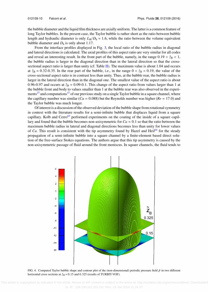
Of interest is a discussion of the observed deviation of the bubble shape from rotational symmetryin context with the literature results for a semi-infinite bubble that displaces liquid from a squarecapillary. Kolb and Cerro63 performed experiments on the coating of the inside of a square capil-lary and found that the bubble becomes non-axisymmetric for Ca ≈ 0.1 so that the ratio between themaximum bubble radius in lateral and diagonal directions becomes less than unity for lower valuesof Ca. This result is consistent with the tip asymmetry found by Hazel and Heil64 for the steadypropagation of a semi-infinite bubble into a square channel by a finite-element based direct solu-tion of the free-surface Stokes equations. The authors argue that this tip asymmetry is caused by thenon-axisymmetric passage of fluid around the front meniscus. In square channels, the fluid tends to

FIG. 4. Computed Taylor bubble shape and contour plot of the (non-dimensional) periodic pressure field p in two differenthorizontal cross sections at zB= 0.15 and 0.325 (results of TURBIT-VOF).


to IP: 134.130.161.251 On: Mon, 18 Jan 2016 11:24:37


move towards the corners, which offer less resistance to the flow than the thinner regions along thechannel sides. The resulting transverse flows induce a transverse pressure gradient that lowers thefluid pressure in the corners, where the air-liquid interface moves radially outwards.64

In view of this, contour-plots of the computed (non-dimensional) periodic pressure field p in ahorizontal cross section are shown in Fig. 4 for two different axial locations (results of TURBIT-VOF).In the cross section at zB = 0.325, the pressure at the channel sides is larger than in the corners,in agreement with Hazel and Heil.64 In contrast, in the cross section at zB = 0.15 (i.e., close to therear meniscus), the pressure at the channel sides is smaller than in the corners. At each point of theinterface, there is in normal direction a balance between capillary, viscous, and pressure forces. Here,normal viscous stresses are expected to be negligible. The non-uniform azimuthal pressure distri-bution in a horizontal cross section is then locally balanced by azimuthally non-uniform capillaryforces. As the coefficient of surface tension is constant in our simulations, this can only be achievedby a change of the local interface curvature which results in the observed deviation of the Taylorbubble shape from rotational symmetry. In Section V, it will be shown that the difference betweenthe maximum bubble radius in lateral and diagonal directions and the axial variation of the bubbleaspect ratio has strong implications on the local flow field in the rear part of the liquid film.

B. Streamlines

Fig. 5 shows streamlines of the flow in a frame of reference moving with the bubble in a lateral anddiagonal cut in combination with a contour-plot of the vertical velocity component in a fixed frame of

FIG. 5. Streamlines in the frame of reference moving with the bubble and vertical velocity in fixed frame of reference (colorcode) in a lateral and diagonal longitudinal cut (results of FS3D).


to IP: 134.130.161.251 On: Mon, 18 Jan 2016 11:24:37


reference (results of FS3D). The streamlines within the bubble indicate the presence of three toroidalvortices. The large central vortex in the body of the Taylor bubble exhibits high upward gas velocitiesclose to the channel axis and low upward velocities close to the interface. This main central vortexdrives two smaller toroidal vortices at the bubble front and bubble rear. The direction of rotation ofboth smaller vortices is opposite to that of the main vortex. The position of the center of the mainvortex differs considerably in the lateral and diagonal cuts. This shows that the flow in the bubble isnot axisymmetric but three-dimensional, especially in the lower part of the main vortex.

In the liquid slug, there is one main toroidal vortex which rotates in the same direction as the mainvortex in the bubble. The occurrence of this recirculation pattern in the liquid phase was postulatedby Taylor65 and was experimentally verified by Cox.66 Also visible is the dividing streamline, whichseparates the liquid slug in two regions, one with recirculating flow in the channel center and one withbypass flow close to the channel walls.17 The knowledge of the position of the dividing streamlineis important for mechanistic modeling of mass transfer in Taylor flow.17,67 In the bypass region, theliquid velocity is low and one can identify in Fig. 5 local areas in the rear part of the liquid film wherethe liquid is flowing downwards.

Visualizations equivalent to Fig. 5 were also made for TURBIT-VOF and DROPS. Though thestreamlines and contour lines are similar to those for FS3D displayed in Fig. 5, there are some notabledifferences in the location of the vortex centers and the radial position of the dividing streamline.These differences partly result from the different post-processing tools used by each code to obtain thestreamlines. Furthermore, in the region near the front and rear menisci, the velocities are very smallin the moving frame of reference (from which the streamlines are computed) so that the evaluationof streamlines becomes inaccurate. This may also explain why the streamlines in these regions arenot closed in Fig. 5.

C. Velocity field in the liquid slug

For a detailed quantitative analysis of the velocity field in the liquid slug, local profiles ofthe axial and radial velocities are shown in Fig. 6 at three different axial positions, where alsoexperimental data are available for comparison. Close to the front and rear menisci, the velocitiesshow strong axial gradients. Therefore, the numerical profiles displayed in Fig. 6 were interpolatedfrom the closest computational nodes to the specific respective axial position. The computed profilesof the axial velocity agree very well in the lateral near wall and corner regions with bypass flow,where they almost overlap for all three axial heights. Differences in the profiles of the axial velocityoccur, however, in the channel center. These can partly be attributed to the different volumetric flowrates of the three codes. According to Table I, the volumetric flow rate of FS3D and DROPS is almostthe same whereas the volumetric flow rate of TURBIT-VOF is about 3% larger. The profiles of theaxial velocity of FS3D and DROPS are virtually identical in Figs. 6(b) and 6(c), while close to thebubble rear a slight difference can be observed in the channel center, see Fig. 6(c). The higher axialvelocity in the channel center computed by TURBIT-VOF (as compared to FS3D and DROPS) inFigs. 6(a) and 6(b) is consistent with its larger volumetric flow rate. Close to the bubble nose, the axialvelocity in the channel center of TURBIT-VOF is, however, smaller as compared to the other codes,while the profile is slightly wider, see Fig. 6(c). In summary, the deviation of the computational andexperimental results for the local centerline axial velocity is about 3%–5% for the three consideredaxial positions, while the deviation between the codes is less than 3%.

The ratio between the maximum and mean axial velocity in the liquid slug is about 1.9. This valueis lower than 2.096, which is the corresponding value of the fully developed laminar flow in a squarechannel. Thus, the liquid slug is not long enough for the velocity profile to become fully developed.This observation is consistent with experimental results from the literature. Cox66 reports a Poiseuillevelocity distribution at a distance of 1.5 tube diameters ahead of the bubble, while Thulasidas et al.17

found that the Poiseuille profile within the liquid slug is fully developed for LS/Dh ≥ 1.5. In thepresent case, the ratio between slug length and hydraulic diameter is only LS/Dh ≈ 0.6.

The comparison of the computed lateral profiles of the axial velocity in the liquid slug with theexperimental data yields a rather sophisticated picture. Close to the bubble rear the agreement is quitegood, Fig. 6(a). The same holds for the magnitude of the axial velocity in the channel center close


to IP: 134.130.161.251 On: Mon, 18 Jan 2016 11:24:37


FIG. 6. Lateral and diagonal profiles of the axial and radial velocities in the liquid slug at different axial positions: (a) closeto bubble rear (zS= 0.9), (b) in the middle of the liquid slug (zS= 0.5), and (c) close to the bubble nose (zS= 0.1).

to the bubble nose, Fig. 6(c). In the middle of the liquid slug, the maximum axial velocity in theexperiment is slightly higher than in the simulations, Fig. 6(b). A rather large deviation between theexperimental data and the numerical profiles occurs close to the channel walls, both in the middle ofthe liquid slug, Fig. 6(b), and close to the bubble nose, Fig. 6(c). In both regions, the numerical results


to IP: 134.130.161.251 On: Mon, 18 Jan 2016 11:24:37


appear to be more reliable than the measured data. Uncertainties in the experimental data arise fromthe temperature dependence of the refractive index. Even minor changes in temperature may lead tooptical refractive index mismatch at the channel wall. It is expected that a further development of theexperimental setup (RIM and temperature control) will improve the accuracy of near wall velocitymeasurements.

Figs. 6(a) and 6(c) also show profiles of the radial liquid velocity in a lateral and diagonal cut. Inthe middle of the liquid slug, the radial velocity is virtually zero; the respective profiles are, therefore,not included in Fig. 6(b). The radial velocity profiles of all three codes are very similar but differslightly in magnitude. Due to the recirculation pattern in the liquid slug (cf. Fig. 5), the radial liquidvelocity is non-zero close to the front and rear menisci. Close to the bubble nose the liquid flows in-ward (i.e., toward the channel axis), while close to the bubble rear the liquid flow is outward. Figs. 6(a)and 6(c) show that at both locations, i.e., zS = 0.1 and 0.9, the magnitude of the radial velocity is onlyabout 10% of the axial velocity.

D. Velocity field in the bubble and the liquid film

Figs. 7(a)–7(c) show similar velocity profiles as in Fig. 6 but for the bubble region. The respectiveaxial positions correspond to zB = 0.25, 0.5, and 0.75. Each velocity profile belongs partly to theliquid film and partly to the gas flow within the bubble. The exact radial positions of the interfacein the lateral and diagonal cuts can be calculated for each code from the data given in Table II. InFigs. 7(a)–7(c), the average bubble diameter of the three codes at the respective axial position ismarked by vertical dashed lines.

First, the velocity profiles inside the bubble are discussed. The results of FS3D and DROPSalmost overlap for zB = 0.25 but deviate by a few percent for zB = 0.5 and 0.75. TURBIT-VOF pre-dicts a smaller magnitude of the axial velocity as compared to FS3D. The deviation in the magnitudeof the computed centerline axial velocity between the different codes at the three considered axialpositions is about 1.5%–5% and is the largest in the bubble nose. These differences are rather large,given the fact that the bubble velocity in all codes is very similar (the corresponding deviation is only0.4%). This can be attributed to the fact that the flow inside the bubble is more complex than that inthe liquid slug.

For sufficiently large values of r/Dh, the profiles in Figs. 7(a)–7(c) correspond to the velocity inthe liquid film (say rD/L/Dh > 0.4-0.48 depending on axial position). First, the results for the radialvelocity are discussed qualitatively. In the diagonal cut, the magnitude of the radial velocity is verysmall close to the walls and the profile for radial velocity exhibits a horizontal tangent for all threeaxial positions. In the lateral cut, the magnitude of the radial velocity close to the wall is larger thanin the diagonal cut and the horizontal tangent exists only for zB = 0.75, see Fig. 7(a). The profiles forzB = 0.25 and 0.5 show that liquid flows towards the wall. This is related to the axial profile of thebubble shape. Namely, the bubble diameter is increasing as zB decreases (cf. Fig. 3), and the bubblepushes liquid toward the wall, where it is redistributed laterally toward the channel corners. Thisresults in a draining of the lateral liquid film which will be discussed further in Section V.

For the axial velocity in the liquid film, experimental results are available for a comparison andincluded in Figs. 7(a)–7(c). The agreement between the three codes and the experimental results israther good, both for the lateral and the diagonal cuts. This indicates that the slight differences in thecomputed bubble shape have only a minor effect on the flow in the liquid film. For zB = 0.75 and 0.5,an upward flow in the liquid film can be observed. For zB = 0.5, the velocity profile in the liquid filmis linear and of “Couette type” as discussed by Meyer et al.44 At zB = 0.25, there is a local backflowof liquid in the film, both in the experiment as well as in the three computations. The magnitude ofthis backflow is much larger in the diagonal cut than in the lateral cut; see the inset in Fig. 7(c). Thisis consistent with the contour-plot of the vertical velocity shown in Fig. 5.

Since this paper considers co-current upward flow, one might conjecture that this local backflowis related to gravitational forces. However, this is not the case as is checked by a simulation with FS3Dfor the same value of UB but without gravitation forces (g = 0). Also in this case, a local backflow inthe rear part of the liquid film is found.


to IP: 134.130.161.251 On: Mon, 18 Jan 2016 11:24:37


FIG. 7. Lateral and diagonal profiles of the axial and radial velocities at different axial positions in the bubble and the liquidfilm: (a) zB= 0.75, (b) zB= 0.5, (c) zB= 0.25. The inset graphics in (b) and (c) show the lateral profiles of the axial velocityclose to the wall. For the legend, see Fig. 6(a). The vertical dashed lines denote the average bubble diameter of the three codesat the respective axial position.

During the passage of a bubble, the local backflow causes a temporal reversal of the sign of thewall shear stress at a fixed position. This is of importance for heat and mass transfer applicationswith Taylor flow in various technical fields. An example in material science is the synthesis of parti-cles with narrow size-distribution.68 In biology and medicine, lab-on-a-chip applications with Taylor


to IP: 134.130.161.251 On: Mon, 18 Jan 2016 11:24:37


flow are of interest for cell stimulus.15 Here, the shear stresses exerted on cells are of importance forthe cell viability.69 In membranes for ultrafiltration, the alternating shear stresses of slug flow are ofbenefit for the cleaning and fouling control.70,71 Taha and Cui29,72 performed in this context numericalsimulations with the volume-of-fluid method in the FLUENT code. They considered a single Taylorbubble in a vertical tube72 (20 mm inner diameter) and in a square capillary29 (Dh = 2 mm) and stud-ied among others the wall shear stress distribution. For the square capillary, they found a reversal ofthe shear stress in lateral and diagonal directions both for upward and downward flows of the Taylorbubble. Moreover, the axial location of the wall shear stress reversal was found to be different in thelateral film and the channel corners. The authors did, however, not discuss the local velocity field inthat region, nor did they give an explanation for the shear stress reversal.

V. ANALYSIS OF LOCAL BACKFLOW IN THE REAR LIQUID FILM

The most interesting result of Section IV is the occurrence of local backflow in the rear part ofthe liquid film. This section provides a physical explanation for this feature and gives criteria for itsoccurrence.

To investigate the phenomenon in more detail, advantage of the full simulation results is taken andthe three-dimensional flow field is visualized at different locations. Fig. 8(a) shows the bubble shape,the isosurface of uz = −16 mm/s, and velocity vectors at the horizontal cross sections zB = 0.17, 0.29,and 0.52 (results of TURBIT-VOF). The velocity vectors indicate that the flow in the liquid film isupward at zB = 0.52 and is downward at zB = 0.29 and 0.17. From the volume enclosed by the iso-surface for uz = −0.16 m/s, it is evident that the backflow region in the liquid film is much larger inthe channel corners than at the channel sides. For the two upper horizontal planes, the velocity in thelateral liquid film is quite small. In contrast, large downward velocities exist in the lowest plane closeto the bubble rear, where the lateral film is the thinnest. The magnitude of the liquid velocity there isas high as the largest velocities in the corner region (cf. the local profiles of uz in Fig. 10 which willbe discussed below).

The local backflow in the rear part of the liquid film is further illustrated in Figs. 9(a) and 9(b),where contour-plots of the vertical velocity uz are displayed for those two axial positions where theliquid film thickness is minimal in diagonal direction (zB = 0.27) and in lateral direction (zB = 0.17),respectively. Both figures confirm that the axial position where uz is minimal is different in both diag-onal directions (cf. Fig. 8). A detailed inspection of the velocity fields displayed in Figs. 9(a) and 9(b)and in Fig. 8(a) indicates for zB = 0.27 a draining liquid flow out of the lateral film into the channel

FIG. 8. Illustration of local backflow in the rear part of the liquid film (results of TURBIT-VOF). Visualization of the bubbleshape, the isosurface of the vertical velocity uz =−16 mm/s, and the velocity field in three different horizontal cross sections.(a) Base case with Ca= 0.1 and (b) comparative case with Ca= 0.23.


to IP: 134.130.161.251 On: Mon, 18 Jan 2016 11:24:37


FIG. 9. (a) Contour plot of the vertical velocity uz in one quarter of the cross section at position zB= 0.27 where the diagonalliquid film is the thinnest (the red line indicates the interface, every 2nd velocity vector is displayed in x- and y-directions,results of TURBIT-VOF). (b) Same but for position zB= 0.17 where the lateral film is the thinnest. (c) Interface profiles incross section zB= 0.27 (red solid line) and zB= 0.17 (blue dashed line) and illustration of the lateral and diagonal liquid filmareas.

corners, in agreement with the numerical study of Hazel and Heil.64 At zB = 0.17 close to the rearmeniscus, the flow direction in the liquid film is opposite, i.e., from the corner regions towards thelateral film.

A useful concept in Taylor flow is a macroscopic material balance of the liquid flow. By consid-ering a cross section where gas and liquid are present and a cross section through the liquid slug, arelation between the average liquid velocity and the bubble velocity can be established.6,73 In a frameof reference moving with the bubble, this mass balance leads — under the assumptions of quasi-steadystate and incompressible phases — to the relation

(J −UB)A = [UF(zB) −UB] AF(zB). (4)

Here, UF(zB) is the average axial velocity in the liquid film in a cross section at a certain axial posi-tion zB, J is the total superficial velocity, A is the area of the channel cross section, and AF(zB) =A − AB(zB) is the cross-sectional area of the liquid phase. Abiev74 pointed out that Eq. (4) implies thatUF becomes negative for AB(zB)/A > J/UB which corresponds to a local flow reversal in the liquidfilm.

For an axisymmetric bubble in a square channel, it is AB/A = πD2B/4D2

h and Eq. (4) yields

UF(zB) =J −UB

π4D2

B(zB)Dh

1 − π4D2

B(zB)D2

h

. (5)

This relation can be used to compute UF(zB) from the axial profile of the bubble diameter DB(zB). Inthe present case, the bubble is not axisymmetric and has slightly different dimensions in lateral anddiagonal directions (cf. Fig. 3 and Table II). Here, the main interest is in the local axial velocity uz inthe lateral and diagonal liquid film regions and not in the mean axial velocity UF. Nevertheless, it isinteresting to evaluate Eq. (5) under the hypothetical assumption that the bubble is axisymmetric, oncewith the lateral bubble diameter profile DB,L(zB) and once with the diagonal bubble diameter profileDB,D(zB) from Fig. 3. Given the similar interface profiles for the three codes, the respective curvesfor UF(zB) are very similar, too. Therefore, in Fig. 10, only the curves computed from the interfaceprofiles of TURBIT-VOF are shown. The figure shows that for both the bubble profile in lateral andin diagonal directions, there is a region where the predicted value of UF is negative which indicatesbackflow. In lateral direction, the predicted axial region with backflow is smaller and located at alower height as compared to the diagonal direction. These results are consistent with the contour-plotof the velocity field of uz in Fig. 5 (from FS3D) and the isosurface for uz = −0.16 m/s in Fig. 8(a)(from TURBIT-VOF). Both figures show that the axial region where uz is negative differs in the lateraland diagonal cuts.

Also shown in Fig. 10 are local velocity profiles of uz in the middle of the lateral and diagonalliquid films (results of TURBIT-VOF). The profiles of uz in the lateral and diagonal liquid films atother radial positions (not shown here) are qualitatively very similar to those displayed in Fig. 10, butdiffer in magnitude. Comparing the profiles of UF and uz in Fig. 10 shows that Eq. (5) predicts the


to IP: 134.130.161.251 On: Mon, 18 Jan 2016 11:24:37


FIG. 10. Vertical profile of the mean axial velocity in the liquid film, UF, as computed by Eq. (5) from the lateral anddiagonal interface profiles, and vertical profile of the local axial velocity uz in the lateral and diagonal liquid films at positionsrL= 0.484 and rD= 0.592, respectively (results from TURBIT-VOF). The two dashed horizontal lines at zB= 0.17 and 0.27indicate the positions where the liquid film thickness is the thinnest in lateral and diagonal directions, respectively.

region with backflow in lateral direction quite well. For the diagonal liquid film, however, the localvelocity profile indicates that the region with backflow is actually located somewhat closer to the rearmeniscus than is predicted by Eq. (5). The reason for this discrepancy is probably the drainage ofthe lateral liquid film and the associated movement of liquid toward the corners which is visible inFig. 9(b) and which is not taken into account by the above simplified analysis.

Next it is investigated why the locations whereUF is minimal differ so much in lateral and diagonaldirections. By taking the derivative of Eq. (4) with respect to zB, one obtains

∂UF(zB)∂zB

=UB −UF(zB)

AF(zB) >0

∂AF(zB)∂zB

. (6)

From Eq. (6) it follows that the axial position where UF is minimal is identical to the position where AFis minimal. For an axisymmetric bubble in a circular pipe, the thickness of the liquid film is uniform inazimuthal direction so that the axial position where UF is minimal is azimuthally unique. In a squarecapillary, the thickness of the liquid film is not uniform within an axial cross section but varies inazimuthal direction. The liquid film is the thinnest in lateral direction and the thickest in diagonaldirection. To account for this, the area of the liquid film is represented as a sum of two parts, i.e.,


to IP: 134.130.161.251 On: Mon, 18 Jan 2016 11:24:37


AF = AF,L + AF,D. Here, AF,L(zB) is the area of the lateral liquid film and AF,D(zB) is the area of the filmin the corner. The experiments by Fries et al.20 for capillary numbers in the range 0.0002-0.01 showthat the corners can contribute with about 70% to the total film area. An exact definition of both areasis, however, difficult. Fig. 9(c) shows the interface profiles in one quarter of the channel cross sectionat the two axial positions where the thickness of the liquid film is minimal in lateral and diagonaldirections, respectively. In the present case, both curves intersect at an angle of 18.5 and AF,L andAF,D are defined accordingly.

By splitting the liquid volumetric flux in two parts (i.e., through area AF,L or AF,D), the liquidmass balance from Eq. (4) becomes

(J −UB)A = UF,L(zB) −UB

AF,L(zB) +

UF,D(zB) −UB

AF,D(zB). (7)

Taking the derivative of Eq. (7) with respect to zB gives

AF,L>0

∂UF,L

∂zB+ AF,D

>0

∂UF,D

∂zB=

UB −UF,D(zB)

>0

∂AF,D

∂zB+

UB −UF,L(zB)

>0

∂AF,L

∂zB. (8)

To discuss the implications of Eq. (8), it is useful to consider again Fig. 10 where three axial re-gions in the liquid film can be distinguished. In region I at the bubble front it is ∂AF,D/∂zB > 0 and∂AF,L/∂zB > 0 (cf. the interface profiles in Fig. 3) so that the right-hand side of Eq. (8) is positive.For this region, one may expect from Eq. (8) ∂UF,L/∂zB > 0 and ∂UF,D/∂zB > 0. In the liquid filmnear the bubble rear (region III) it is ∂AF,L/∂zB < 0 and ∂AF,D/∂zB < 0 so that the right-hand side ofEq. (8) is negative. In this region, one may expect from Eq. (8) ∂UF,L/∂zB < 0 and ∂UF,D/∂zB < 0.Of special interest here is region II where ∂AF,L/∂zB ≥ 0 and ∂AF,D/∂zB ≤ 0. The magnitude of UF,Land UF,D in this region is about one order smaller than that of UB. Therefore, in the right-hand sideof Eq. (8), the approximations UB −UF,D(zB) ≈ UB and UB −UF,L(zB) ≈ UB can be introduced whichyields

AF,D∂UF,D

∂zB≈ UB

∂AF

∂zB− AF,L

∂UF,L

∂zB. (9)

This equation establishes a relation between the axial derivatives of the mean velocity in the lateraland diagonal liquid films. For the present case, the local profile of uz in the lateral film in Fig. 10 indi-cates that in the entire region II it is ∂UF,L/∂zB ≥ 0. Somewhere within region II, the film area AF(zB)takes its minimum value. Thus, within region II there are two sub-regions, one where ∂AF/∂zB < 0(close to region III) and one where ∂AF/∂zB > 0 (close to region I). In the former sub-region, theright-hand side of Eq. (9) is negative; thus it follows ∂UF,D/∂zB < 0 and the vertical derivatives of themean velocity in the liquid film in lateral and diagonal directions have opposite signs. This behavioris clearly reflected by the local profiles of uz in the lateral and diagonal films in Fig. 10. In the lattersub-region of region II, the right-hand side of Eq. (9) may be positive or negative and a clear statementabout the sign of the derivate ∂UF,D/∂zB is not possible.

In summary, it follows by a mass balance of the liquid flow in the corner and at the channel sidesthat it is the axial change of AF,L and AF,D displayed in Fig. 9(c) which gives rise to region II in Fig. 10with different axial locations where uz is minimal (and negative) in lateral and diagonal directions.The axial change of AF,L and AF,D in the rear part of the liquid film is related to the axial variation ofthe bubble aspect ratio which is caused by the non-uniform azimuthal pressure distribution within across section (cf. Section IV A and Fig. 4).

An implication of the conjecture from the last paragraph is that the size of region II shoulddiminish or even disappears for Taylor bubbles with higher capillary number since these are axisym-metric. This is tested by the comparative simulation, where Ca = 0.23 (cf. last paragraph in Sec. III C).For this comparative case, the ratio between the maximum lateral and maximum diagonal bubble radiiis 0.99 as compared to 0.98 for the base case. Furthermore, the relative difference between the axialpositions where both maxima occur (i.e., the length of region II) takes a value of ∆zB/Dh = 0.080while it was 0.175 for the base case. Fig. 8(b) shows for the comparative case a visualization equivalentto the one displayed in Fig. 8(a) for the base case (where Ca = 0.1). The maximum local downwardvelocity occurs within the isosurface for uz = −16 mm/s. Both in Figs. 8(a) and 8(b), the isosurfacevolume is larger in the corners than in the lateral film. However, in contrast to Fig. 8(a), the isosurface


to IP: 134.130.161.251 On: Mon, 18 Jan 2016 11:24:37


forms in Fig. 8(b) a connected tube around the bubble and the axial position of the isosurface is aboutthe same in the lateral and diagonal films. The downward velocity vectors in Fig. 8(a) increase inmagnitude from the plane at zB = 0.29 to the one at 0.17 in the lateral film, but decrease in the diagonalfilm. In Fig. 8(b), the downward velocity vectors increase in magnitude from the plane at zB = 0.25to the one at 0.17, both in the lateral and the diagonal films. Thus, there is no region visible where theaxial gradients of the axial velocity show opposite signs in the lateral and diagonal films. This andthe significant decrease of the size of region II as the capillary number is increased from Ca = 0.1to 0.23 confirm the conjecture from the previous paragraph. Finally, it is worth to remark that evenfor Ca = 0.23 the Taylor bubble is still locally non-axisymmetric. Similar to the base case, the ratiobetween the local lateral and diagonal bubble diameter is larger than unity close to the rear meniscus(with a maximum of about 1.04), while it is smaller than unity at the bubble body and nose (with aminimum value of about 0.97). Thus, as compared to the base case, this local deviation from rotationalsymmetry has decreases as well, as did the global deviation from rotational symmetry (measured bythe ratio of the maximum lateral to maximum diagonal bubble radius).

For practical applications with Taylor flow it may be useful to estimate beforehand whether alocal backflow in the liquid film is to be expected or not. From Eq. (4), it follows that a sufficientcondition for local backflow is

AB,max

A· UB

J> 1, (10)

where AB,max is the maximum value of the cross-sectional area of the bubble. The first ratio on theleft-hand side of Eq. (10) is always less than unity, whereas the second ratio is always larger than unity.Both ratios depend on the capillary number. Liu et al.19 performed experiments in capillaries withcircular and square cross section for various fluids and derived a correlation for UB/J. For circularchannels, the correlation of Abiev67 for UB/J (which is valid for a wider range of capillary numbers)can be used as well while the ratio AB,max/A can be estimated from the correlation of Aussillous andQuere75 for the liquid film thickness. This allows to test the inequality in Eq. (10) for circular channels.

For square channels, the determination of AB,max/A is more subtle and one has to distinguish be-tween globally axisymmetric bubbles and globally non-axisymmetric bubbles. According to Kreutzeret al.,11 the transition between both regimes occurs at Ca ≈ 0.04. The latter authors provide a correla-tion for the bubble diameter in the axisymmetric regime. For the non-axisymmetric regime, they pro-vide correlations for the bubble diameter in lateral and diagonal directions. For the non-axisymmetriccase, these correlations allow in combination with the geometrical considerations reported in the ap-pendix of Kolb and Cerro63 to estimate AB,max/A and thus to test the criterion in Eq. (10). Alternatively,one can use the correlation for AB given by Haase and Bauer23 which is based on the assumptionDB,max;L/Dh = 0.95. In the present simulations, the latter ratio has a value of about 0.93. Finally, itis noted that in the present study and in our previous one37 the bubble is already slightly globallynon-axisymmetric for Ca ≈ 0.1. If the Taylor bubble in a square channel is not globally axisymmetric,then the local backflow in the lateral and diagonal film will occur in different axial regions as shownabove.

VI. CONCLUSIONS

This paper presents a coordinated numerical and experimental study on local flow phenomenain co-current upward laminar Taylor flow through a small square channel. In the computations withthree academic computer codes, the bubble volume and velocity as well as the size of the Taylor flowunit cell are chosen in accordance with the experiments (with values of the capillary and Reynoldsnumber of 0.1 and 7, respectively). For these parameters, the local numerical results for the bubbleradius agree with a deviation of about 0.6%. For the local centerline axial velocity, the results agreewith a deviation of less than 3% in the liquid slug and of less than about 5% for the flow within thebubble.

Parameters which are sensitive with respect to the numerical method are the minimum thick-ness of the lateral liquid film and the axial position where the minimum thickness occurs. Whilethe agreement regarding the bubble shape and the velocity field in the liquid slug and in the liquidfilm is reasonably good, the differences concerning the flow in the bubble are larger. From this, one


to IP: 134.130.161.251 On: Mon, 18 Jan 2016 11:24:37


can conclude that a reasonable good agreement for the bubble shape and bubble velocity does notautomatically imply a good agreement in the local velocity field within the bubble. The reasons forthe rather large discrepancies concerning the flow within the bubble are yet unclear. Uncovering themrequires detailed experimental data on the velocity field within the Taylor bubble as well as furthercomputational studies and benchmark data on the local velocity and pressure fields within the Taylorbubble.

The present experimental and computational results consistently show a local backflow regionin the rear part of the liquid film in the fixed frame of reference. This is associated with a temporalreversal of the wall shear stress during the passage of a Taylor bubble. This local backflow occursat different axial positions in the lateral film and in the corner region. By a detailed analysis of thefull three-dimensional simulation results, it is shown that this novel phenomenon has its origin in aslight deviation of the Taylor bubble shape from rotational symmetry. Of special importance is thecrossover of the local bubble aspect ratio (defined as the local ratio between the bubble diameter indiagonal and lateral directions at a certain axial position) from values larger than unity at the bubblenose and bubble body to values smaller than unity at the bubble rear.

Our study considered two specific values of the capillary number. Future studies may investigatethe existence and size of this local backflow region for capillary and Reynolds numbers varying ina wider range. So far, approximate criteria are given for the conditions under which the shear stressreversal occurs in circular and square channels. These and the detailed understanding of the underly-ing physical mechanism shall be useful for some technical applications with gas-liquid Taylor flow(e.g., material synthesis). Finally, it is likely that similar phenomena will also occur in channels withother polygonal cross section, such as trapezoidal or equilateral triangular channels.

ACKNOWLEDGMENTS

The authors wish to thank the German Research Foundation (DFG) for financial support withinthe Priority Programme “Transport Processes at Fluidic Interfaces” (SPP 1506) with the Project Nos.BO 1879/9-1, RE 1461/2-1, SCHL 617/7-1, and WO 1682/1-1.

1 S. Osher and R. P. Fedkiw, Level Set Methods and Dynamic Implicit Surfaces (Springer, Berlin, London, 2003).2 G. Tryggvason, R. Scardovelli, and S. Zaleski, Direct Numerical Simulations of Gas-Liquid Multiphase Flows (Cambridge

University Press, Cambridge, 2011).3 A. Prosperetti and G. Tryggvason, Computational Methods for Multiphase Flow (Cambridge University Press, Cambridge,

2007).4 S. Groß and A. Reusken, Numerical Methods for Two-Phase Incompressible Flows (Springer, Heidelberg, 2011).5 M. Wörner, “Numerical modeling of multiphase flows in microfluidics and micro process engineering: A review of methods

and applications,” Microfluid. Nanofluid. 12, 841 (2012).6 M. Suo and P. Griffith, “Two-phase flow in capillary tubes,” J. Basic Eng. 86, 576 (1964).7 D. T. Dumitrescu, “Strömung an einer luftblase im senkrechten Rohr,” Z. Angew. Math. Mech. 23, 139 (1943).8 R. M. Davies and G. Taylor, “The mechanics of large bubbles rising through extended liquids and through liquids in tubes,”

Proc. R. Soc. A 200, 375 (1950).9 K. Jähnisch, M. Baerns, V. Hessel, W. Ehrfeld, V. Haverkamp, H. Löwe, C. Wille, and A. Guber, “Direct fluorination of

toluene using elemental fluorine in gas/liquid microreactors,” J. Fluorine Chem. 105, 117 (2000).10 M. Al-Rawashdeh, J. Zalucky, C. Muller, T. A. Nijhuis, V. Hessel, and J. C. Schouten, “Phenylacetylene hydrogenation over

[Rh(NBD)(PPh3)2]BF4 catalyst in a numbered-up microchannels reactor,” Ind. Eng. Chem. Res. 52, 11516 (2013).11 M. T. Kreutzer, F. Kapteijn, J. A. Moulijn, and J. J. Heiszwolf, “Multiphase monolith reactors: Chemical reaction engineering

of segmented flow in microchannels,” Chem. Eng. Sci. 60, 5895 (2005).12 A. Günther and K. F. Jensen, “Multiphase microfluidics: From flow characteristics to chemical and materials synthesis,”

Lab Chip 6, 1487 (2006).13 J. I. Park, A. Saffari, S. Kumar, A. Günther, and E. Kumacheva, “Microfluidic synthesis of polymer and inorganic particulate

materials,” Annu. Rev. Mater. Res. 40, 415 (2010).14 J. M. Köhler, S. N. Li, and A. Knauer, “Why is micro segmented flow particularly promising for the synthesis of nanoma-

terials?,” Chem. Eng. Technol. 36, 887 (2013).15 J. El-Ali, S. Gaudet, A. Günther, P. K. Sorger, and K. F. Jensen, “Cell stimulus and lysis in a microfluidic device with

segmented gas-liquid flow,” Anal. Chem. 77, 3629 (2005).16 T. C. Thulasidas, M. A. Abraham, and R. L. Cerro, “Bubble-train flow in capillaries of circular and square cross-section,”

Chem. Eng. Sci. 50, 183 (1995).17 T. C. Thulasidas, M. A. Abraham, and R. L. Cerro, “Flow patterns in liquid slugs during bubble-train flow inside capillaries,”

Chem. Eng. Sci. 52, 2947 (1997).18 T. Cubaud and C. M. Ho, “Transport of bubbles in square microchannels,” Phys. Fluids 16, 4575 (2004).


to IP: 134.130.161.251 On: Mon, 18 Jan 2016 11:24:37

http://dx.doi.org/10.1007/s10404-012-0940-8

http://dx.doi.org/10.1115/1.3653176

http://dx.doi.org/10.1002/zamm.19430230303

http://dx.doi.org/10.1098/rspa.1950.0023

http://dx.doi.org/10.1016/S0022-1139(00)00300-6

http://dx.doi.org/10.1021/ie4009277

http://dx.doi.org/10.1016/j.ces.2005.03.022

http://dx.doi.org/10.1039/b609851g

http://dx.doi.org/10.1146/annurev-matsci-070909-104514

http://dx.doi.org/10.1002/ceat.201200695

http://dx.doi.org/10.1021/ac050008x

http://dx.doi.org/10.1016/0009-2509(94)00225-G

http://dx.doi.org/10.1016/S0009-2509(97)00114-0

http://dx.doi.org/10.1063/1.1813871


19 H. Liu, C. O. Vandu, and R. Krishna, “Hydrodynamics of Taylor flow in vertical capillaries: Flow regimes, bubble risevelocity, liquid slug length, and pressure drop,” Ind. Eng. Chem. Res. 44, 4884 (2005).

20 D. M. Fries, F. Trachsel, and P. R. von Rohr, “Segmented gas-liquid flow characterization in rectangular microchannels,”Int. J. Multiphase Flow 34, 1108 (2008).

21 M. J. F. Warnier, E. Rebrov, M. H. J. M. De Croon, V. Hessel, and J. C. Schouten, “Gas hold-up and liquid film thicknessin Taylor flow in rectangular microchannels,” Chem. Eng. J. 135, S153 (2008).

22 Y. Han and N. Shikazono, “Measurement of liquid film thickness in micro square channel,” Int. J. Multiphase Flow 35, 896(2009).

23 S. Haase and T. Bauer, “New method for simultaneous measurement of hydrodynamics and reaction rates in a mini-channelwith Taylor flow,” Chem. Eng. J. 65, 176–177 (2011).

24 M. Roudet, K. Loubiere, C. Gourdon, and M. Cabassud, “Hydrodynamic and mass transfer in inertial gas-liquid flow regimesthrough straight and meandering millimetric square channels,” Chem. Eng. Sci. 66, 2974 (2011).

25 P. Zaloha, J. Kristal, V. Jiricny, N. Volkel, C. Xuereb, and J. Aubin, “Characteristics of liquid slugs in gas-liquid Taylor flowin microchannels,” Chem. Eng. Sci. 68, 640 (2012).

26 T. Abadie, J. Aubin, D. Legendre, and C. Xuereb, “Hydrodynamics of gas-liquid Taylor flow in rectangular microchannels,”Microfluid. Nanofluid. 12, 355 (2012).

27 S. Boden, T. dos Santos Rolo, T. Baumbach, and U. Hampel, “Synchrotron radiation microtomography of Taylor bubblesin capillary two-phase flow,” Exp. Fluids 55, 1 (2014).

28 B. E. Ghidersa, M. Wörner, and D. G. Cacuci, “Exploring the flow of immiscible fluids in a square vertical mini-channelby direct numerical simulation,” Chem. Eng. J. 101, 285 (2004).

29 T. Taha and Z. F. Cui, “CFD modelling of slug flow inside square capillaries,” Chem. Eng. Sci. 61, 665 (2006).30 M. Wörner, B. Ghidersa, and A. Onea, “A model for the residence time distribution of bubble-train flow in a square

mini-channel based on direct numerical simulation results,” Int. J. Heat Fluid Flow 28, 83 (2007).31 D. S. Liu and S. D. Wang, “Hydrodynamics of Taylor flow in noncircular capillaries,” Chem. Eng. Process. 47, 2098 (2008).32 M. C. Öztaskin, M. Wörner, and H. S. Soyhan, “Numerical investigation of the stability of bubble train flow in a square

minichannel,” Phys. Fluids 21, 042108 (2009).33 A. Onea, M. Wörner, and D. G. Cacuci, “A qualitative computational study of mass transfer in upward bubble train flow

through square and rectangular mini-channels,” Chem. Eng. Sci. 64, 1416 (2009).34 S. Kececi, M. Wörner, A. Onea, and H. S. Soyhan, “Recirculation time and liquid slug mass transfer in co-current upward

and downward Taylor flow,” Catal. Today 147, S125 (2009).35 O. Keskin, M. Wörner, H. S. Soyhan, T. Bauer, O. Deutschmann, and R. Lange, “Viscous co-current downward Taylor flow

in a square mini-channel,” AIChE J. 56, 1693 (2010).36 M. Wörner, “Computational study on scaling of co-current downward Taylor flow in small square channels of three different

sizes,” J. Chem. Eng. Jpn. 46, 335 (2013).37 H. Marschall, S. Boden, C. Lehrenfeld, C. J. D. Falconi, U. Hampel, A. Reusken, M. Wörner, and D. Bothe, “Validation

of interface capturing and tracking techniques with different surface tension treatments against a Taylor bubble benchmarkproblem,” Comput. Fluids 102, 336 (2014).

38 P. Angeli and A. Gavriilidis, “Hydrodynamics of Taylor flow in small channels: A review,” Proc. Inst. Mech. Eng., Part C222, 737 (2008).

39 R. Gupta, D. F. Fletcher, and B. S. Haynes, “Taylor flow in microchannels: A review of experimental and computationalwork,” J. Comput. Multiphase Flows 2, 1 (2010).

40 P. Sobieszuk, J. Aubin, and R. Pohorecki, “Hydrodynamics and mass transfer in gas-liquid flows in microreactors,” Chem.Eng. Technol. 35, 1346 (2012).

41 V. Talimi, Y. S. Muzychka, and S. Kocabiyik, “A review on numerical studies of slug flow hydrodynamics and heat transferin microtubes and microchannels,” Int. J. Multiphase Flow 39, 88 (2012).

42 S. Aland, C. Lehrenfeld, H. Marschall, C. Meyer, and S. Weller, “Accuracy of two-phase flow simulations: The Taylor flowbenchmark,” PAMM 13, 595 (2013).

43 S. Aland, S. Boden, A. Hahn, F. Klingbeil, M. Weismann, and S. Weller, “Quantitative comparison of Taylor flow simulationsbased on sharp-interface and diffuse-interface models,” Int. J. Numer. Methods Fluids 73, 344 (2013).

44 C. Meyer, M. Hoffmann, and M. Schlüter, “Micro-PIV analysis of gas–liquid Taylor flow in a vertical oriented square shapedfluidic channel,” Int. J. Multiphase Flow 67, 140 (2014).

45 S. P. Quan, “Co-current flow effects on a rising Taylor bubble,” Int. J. Multiphase Flow 37, 888 (2011).46 M. Rieber, “Numerische modellierung der dynamik freier grenzflächen in zweiphasenströmungen,” Fortschrittberichte

VDI/7, VDI-Verlag, 2003.47 R. B. DeBar, “Fundamentals of the KRAKEN code. [Eulerian hydrodynamics code for compressible nonviscous flow of

several fluids in two-dimensional (axially symmetric) region],” Technical Report UCID-17366 Lawrence Livermore Lab.CA, 1974.

48 C. W. Hirt and B. D. Nichols, “Volume of fluid (VOF) method for the dynamics of free boundaries,” J. Comput. Phys. 39,201 (1981).

49 W. J. Rider and D. B. Kothe, “Reconstructing volume tracking,” J. Comput. Phys. 141, 112 (1998).50 D. Bothe, M. Kröger, and H.-J. Warnecke, “A VOF-based conservative method for the simulation of reactive mass transfer

from rising bubbles,” Fluid Dyn. Mater. Process. 7, 303 (2011).51 D. Bothe and S. Fleckenstein, “A volume-of-fluid-based method for mass transfer processes at fluid particles,” Chem. Eng.

Sci. 101, 283 (2013).52 C. Gotaas, P. Havelka, H. A. Jakobsen, H. F. Svendsen, M. Hase, N. Roth, and B. Weigand, “Effect of viscosity on

droplet-droplet collision outcome: Experimental study and numerical comparison,” Phys. Fluids 19, 102106 (2007).53 C. Focke and D. Bothe, “Direct numerical simulation of binary off-center collisions of shear thinning droplets at high Weber

numbers,” Phys. Fluids 24, 073105 (2012).


to IP: 134.130.161.251 On: Mon, 18 Jan 2016 11:24:37

http://dx.doi.org/10.1021/ie049307n

http://dx.doi.org/10.1016/j.ijmultiphaseflow.2008.07.002

http://dx.doi.org/10.1016/j.cej.2007.07.008





http://dx.doi.org/10.1007/s10404-011-0880-8

http://dx.doi.org/10.1007/s00348-014-1768-7



http://dx.doi.org/10.1016/j.ijheatfluidflow.2006.04.011

http://dx.doi.org/10.1016/j.cep.2007.10.025

http://dx.doi.org/10.1063/1.3101146


http://dx.doi.org/10.1016/j.cattod.2009.07.054

http://dx.doi.org/10.1002/aic.12113

http://dx.doi.org/10.1252/jcej.12we068

http://dx.doi.org/10.1016/j.compfluid.2014.06.030

http://dx.doi.org/10.1243/09544062jmes776

http://dx.doi.org/10.1260/1757-482X.2.1.1




http://dx.doi.org/10.1002/pamm.201310278

http://dx.doi.org/10.1002/fld.3802



http://dx.doi.org/10.2172/7227630

http://dx.doi.org/10.2172/7227630

http://dx.doi.org/10.1016/0021-9991(81)90145-5

http://dx.doi.org/10.1006/jcph.1998.5906

http://dx.doi.org/10.3970/fdmp.2011.007.303



http://dx.doi.org/10.1063/1.2781603

http://dx.doi.org/10.1063/1.4737582


54 C. Albert, H. Raach, and D. Bothe, “Influence of surface tension models on the hydrodynamics of wavy laminar fallingfilms in volume of fluid-simulations,” Int. J. Multiphase Flow 43, 66 (2012).

55 W. Sabisch, “Dreidimensionale numerische simulation der dynamik von aufsteigenden einzelblasen und blasenschwärmenmit einer volume-of-fluid-methode,” Ph.D. thesis, University Karlsruhe, 2000.

56 S. Groß and A. Reusken, “Finite element discretization error analysis of a surface tension force in two-phase incompressibleflows,” SIAM J. Numer. Anal. 45, 1679 (2007).

57 S. Groß, J. Peters, V. Reichelt, and A. Reusken, The DROPS package for numerical simulations of incompressible flowsusing parallel adaptive multigrid techniques, RWTH Aachen University, 2002, IGPM Report No. 211.

58 E. Bertakis, S. Gross, J. Grande, O. Fortmeier, A. Reusken, and A. Pfennig, “Validated simulation of droplet sedimentationwith finite-element and level-set methods,” Chem. Eng. Sci. 65, 2037 (2010).

59 M. Wörner, B. Ghidersa, and A. Shahab, Numerical Study of Bubble Train Flow in a Square Vertical Mini-Channel: Influenceof the Length of the Flow Unit Cell (Proc. 5th Int. Conf. Multiphase Flow ICMF-2004, Yokohama, Japan, 2004).

60 M. R. Ozgu, J. C. Chen, and A. H. Stenning, “Local liquid film thickness around Taylor bubbles,” J. Heat Transfer 95, 425(1973).

61 L. W. Schwartz, H. M. Princen, and A. D. Kiss, “On the motion of bubbles in capillary tubes,” J. Fluid Mech. 172, 259(1986).

62 E. Klaseboer, R. Gupta, and R. Manica, “An extended Bretherton model for long Taylor bubbles at moderate capillarynumbers,” Phys. Fluids 26, 032107 (2014).

63 W. B. Kolb and R. L. Cerro, “Coating the inside of a capillary of square cross section,” Chem. Eng. Sci. 46, 2181 (1991).64 A. L. Hazel and M. Heil, “The steady propagation of a semi-infinite bubble into a tube of elliptical or rectangular cross-

section,” J. Fluid Mech. 470, 91 (2002).65 G. I. Taylor, “Deposition of a viscous fluid on the wall of a tube,” J. Fluid Mech. 10, 161 (1961).66 B. G. Cox, “An experimental investigation of the streamlines in viscous fluid expelled from a tube,” J. Fluid Mech. 20, 193

(1964).67 R. S. Abiev, “Bubbles velocity Taylor circulation rate and mass transfer model for slug flow in milli- and microchannels,”

Chem. Eng. J. 227, 66 (2013).68 B. K. H. Yen, A. Günther, M. A. Schmidt, K. F. Jensen, and M. G. Bawendi, “A microfabricated gas-liquid segmented flow

reactor for high-temperature synthesis: The case of CdSe quantum dots,” Angew. Chem., Int. Ed. 44, 5447 (2005).69 J. Hua, L. E. Erickson, T.-Y. Yiin, and L. A. Glasgow, “A review of the effects of shear and interfacial phenomena on cell

viability,” Crit. Rev. Biotechnol. 13, 305 (1993).70 M. Mercier, C. Fonade, and C. Lafforgue-Delorme, “How slug flow can enhance the ultrafiltration flux in mineral tubular

membranes,” J. Membr. Sci. 128, 103 (1997).71 N. Ratkovich, C. C. V. Chan, P. R. Berube, and I. Nopens, “Experimental study and CFD modelling of a two-phase slug

flow for an airlift tubular membrane,” Chem. Eng. Sci. 64, 3576 (2009).72 T. Taha and Z. F. Cui, “CFD modelling of slug flow in vertical tubes,” Chem. Eng. Sci. 61, 676 (2006).73 R. A. S. Brown and G. W. Govier, “Mechanics of large gas bubbles in tubes: II. Prediction of voidage in verticle gas-liquid

flow,” Can. J. Chem. Eng. 43, 224 (1965).74 R. S. Abiev, “Simulation of the slug flow of a gas-liquid system in capillaries,” Theor. Found. Chem. Eng. 42, 105 (2008).75 P. Aussillous and D. Quere, “Quick deposition of a fluid on the wall of a tube,” Phys. Fluids 12, 2367 (2000).


to IP: 134.130.161.251 On: Mon, 18 Jan 2016 11:24:37


http://dx.doi.org/10.1137/060667530


http://dx.doi.org/10.1115/1.3450082

http://dx.doi.org/10.1017/S0022112086001738

http://dx.doi.org/10.1063/1.4868257

http://dx.doi.org/10.1016/0009-2509(91)85119-I

http://dx.doi.org/10.1017/s0022112002001830

http://dx.doi.org/10.1017/S0022112061000159

http://dx.doi.org/10.1017/S0022112064001148


http://dx.doi.org/10.1002/anie.200500792

http://dx.doi.org/10.3109/07388559309075700

http://dx.doi.org/10.1016/S0376-7388(96)00317-1



http://dx.doi.org/10.1002/cjce.5450430502

http://dx.doi.org/10.1134/S0040579508020012

http://dx.doi.org/10.1063/1.1289396

Documents

Numerical and experimental analysis of local flow