Estimating the Severity of the WikiLeaks United StatesDiplomatic Cables Disclosure∗
Michael Gill† Arthur Spirling‡
December 19, 2014
Prepared for PA Letters
Abstract
In November 2010, the WikiLeaks organization began the release of over 250, 000 diplo-matic cables sent by US embassies to the US State Department, uploaded to its websiteby (then) Private Manning, an intelligence analyst with the US Army. This leak waswidely condemned, including by the then Secretary of State, Hillary Clinton. We assessthe severity of the leak by considering the size of the disclosure relative to all diplo-matic cables that were in existence at the time—a quantity that is not known outsideof official sources. We rely on the fact that the cables that were leaked are internallyindexed in such a way that they may be treated as a sample from a discrete uniform dis-tribution with unknown maximum; this is a version of the well known “German TankProblem”. We consider three estimators that rely on discrete uniformity—maximumlikelihood, Bayesian and frequentist unbiased minimum variance—and demonstratethat the results are very similar in all cases. To supplement these estimators, we em-ploy a regression-based procedure that incorporates the timing of cables’ release inaddition to their observed serial numbers. We estimate that, overall, approximately5% of all cables from this timeframe were leaked, but that this number varies consid-erably at the embassy-year level. Our work provides a useful characterization of thesample of documents available to international relations scholars interested in testingtheories of ‘private information’, while helping to inform the public debate surroundingManning’s trial and thirty-five year prison sentence.
∗December 19, 2014. Jonathan Bennett and Michael Egesdal provided helpful comments on an earlierdraft. We are grateful to the Office of the General Counsel at Harvard University for legal advice. Replicationmaterials (code, not data) for the estimators we describe can be found in the Political Analysis archive.†Department of Government, Harvard University. [email protected]‡Department of Government, Harvard University. [email protected]
1
1 Motivation
For scholars of international relations, the WikiLeaks US diplomatic cable disclosure of 2010
is a promising source of data on the American government’s beliefs and strategies as they
pertain to interactions with other states. A mainstay of the now “dominant” (Lake, 2010)
‘rationalist’ approach to war (Fearon, 1995), this type of ‘private information’ is by its very
nature difficult to obtain for analysts: it may never be released on the grounds that to do so
would damage national interests, endanger its citizens (though see Shapiro and Siegel, 2010,
for discussion) or more cynically, because it might allow popular challenge to elite control of
foreign policy (Gibbs, 1995). While this has not necessarily prevented data-driven scholar-
ship on the canonical bargaining model of conflict (e.g. Fearon, 1994b; Werner, 1999; Reed,
2003; Smith and Stam, 2004; Ramsay, 2008; Reiter, 2009) or historical case studies of impor-
tant incidences of decision-making (e.g. Goemens, 2000; Snyder and Borghard, 2011), it does
mean that such work cannot directly examine all the incentives faced, and actions taken,
by leaders in the contemporary period. Precisely because it contains documents that were
not designed for public release and thus are surely more candid about particular political
relationships, the WikiLeaks disclosure potentially represents a trove of data that might be
tapped to test subtle theories in international relations. These include hypotheses regarding
‘audience costs’ (Fearon, 1994a) and the signaling of resolve (see e.g. Smith, 1998; Schultz,
1999; Slantchev, 2006).
As with any ‘new’ data source, it is helpful to understand the nature of the sample available
for researchers before they conduct statistical analysis. A fundamental question in this re-
spect is the size—i.e., the ‘severity’—of the leak (sample) relative to all cables available (the
population) at the time. If this sample is ‘small’—and far from the universe of cases—then
some caution is required in interpreting results using the documents. This is especially true
2
when examining particular embassies (in particular countries) in particular years for which
the data is necessarily more finely sliced. For example, if researchers have an interest in
recent US diplomatic policy in certain areas of the world (e.g. Christensen, 2006), the utility
of studying the disclosed cables presumably varies according to the density of their coverage:
here, knowing that one has access to 5% of all instructions given to ambassadors is very
different to having 95% or 100% of those orders. Furthermore, knowledge of population size
is helpful since it prompts further investigation of the sampling process itself: that is, it
encourages analysts to think carefully about possible selection biases—especially for data
such as these that were not systematically released according to well known bureaucratic
rules—and adjust for them in their statistical approaches.
Quite separate to these methodological concerns, the Manning case received widespread
public attention and broader interest, including accusations of inhumane treatment from the
United Nations special rapporteur on torture.1 Whether or not Manning’s sentence was just
depends in part on the purported severity of the crimes she committed, and in part on the
normatively appropriate relationship between the state and secrecy—a topic of recent inter-
est to political theorists (see Sagar, 2013). Since this Letter may be seen as an attempt to
measure the first of these issues, we see it as a contribution to the public debate surrounding
the trial.
2 Data
The WikiLeaks data consist of 251,237 diplomatic cables sent by the US State Department
to US embassies and missions around the world. Machine readable versions of these docu-
ments are available at various websites, but what is not known to researchers is the fraction
1“Bradley Manning’s treatment was cruel and inhuman, UN torture chief rules”, The Guardian March12, 2012.
3

of all cables in existence that the leak represents. The original data date range is from 1966
to 2010 but we focus on all cables released on or after January 1, 2005. We do this because
coverage prior to the year 2005 is sparse (there are approximately as many cables from 2005–
2010 as there from 1966–2005); second, because we wished to guard against any change in
protocols—concerning the nature of the cables—that the terrorist attacks of September 11,
2001 may have ushered in and that we assume were in full force by 2005. This leaves 163, 958
cables.
Cables are classified into three categories, depending on the degree of damage to national
security that “the unauthorized disclosure of which reasonably could be expected to cause.”2
In descending order of the purported balefulness of unauthorized release, these categories
are ‘Top Secret’,3 ‘Secret’ and ‘Confidential’. Any cable not meeting the criteria for such
restricted access is ‘Unclassified’.
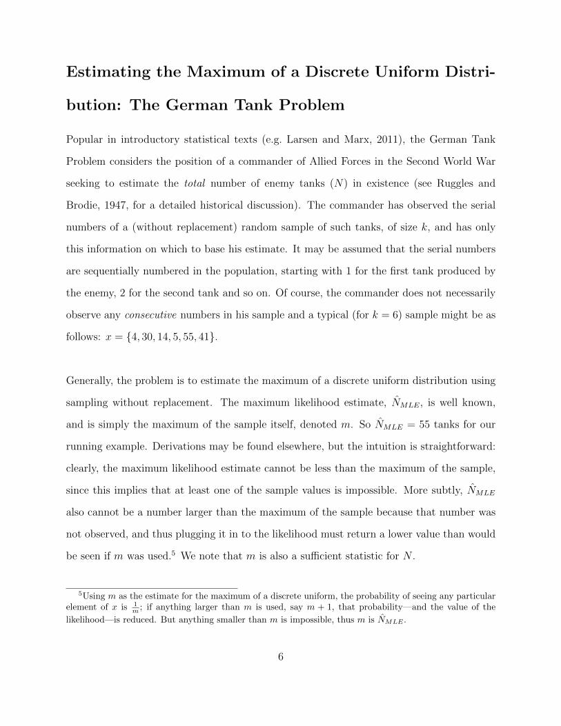
From inspection we note that the cable titles, known internally as the ‘Reference ID’s,
follow a consistent naming convention. Examples of this pattern can be seen in Table 1: a
sample from the US Embassy in Tokyo, for 2009. Consider the Reference ID 09TOKYO13:
the first two digits connote the year of creation (2009) (confirmed by the date ‘Created’
column—information that we culled from the original cable texts); this is followed by the
issuing embassy (TOKYO); followed by a number (13). This particular cable was unclassified,
as can be seen in the third column. Our immediate concern is whether the ‘13’ demarcates
that this was, indeed, the 13th document sent by the Embassy that year, and thus whether
we can treat all such numbers as indicative of their position in the creation order. Our
primary check on this logic was to plot the document numbers against the dates of issue
2Executive Order 13526, 2009.3None of our data has this classification.
4
Reference.ID Date Created Classification09TOKYO4 1/2/09 CONFIDENTIAL
09TOKYO8 1/5/09 UNCLASSIFIED
09TOKYO12 1/5/09 UNCLASSIFIED
09TOKYO13 1/5/09 UNCLASSIFIED
09TOKYO15 1/6/09 UNCLASSIFIED
09TOKYO17 1/6/09 UNCLASSIFIED
09TOKYO20 1/6/09 UNCLASSIFIED
Table 1: Example of Reference ID naming convention: two digit year, followed by Embassyorigin, followed by cable number.
(column 2) for a sample of embassies, and verify that higher numbers appear on later dates.
With some rare exceptions, this is the case.4 Where it is not the case, the reason is likely one
or more of the following: multiple cables are sent from the same embassy on the same day;
cables of different secrecy statuses are processed or cleared at different rates; it takes longer
for some cables to be started and completed than others; there is some mild seasonality in
the rate at which embassies write cables. We do not know why some cables are missing from
the leak; for example, the sample implied by Table 1 is {4, 8, 12, 13, 15, 17, 20}, implying
that cables with numbers 5, 6, 7, 9, 10 etc were written but not leaked. Two possibilities
seem plausible: Manning had limited security clearance, and the ‘unobserved’ cables were
classified as being unavailable at his grade (e.g., this includes those classified as ‘top secret’);
alternatively, Manning was not systematic in gathering the cables and thus we receive a de
facto random sample of those available.
If the cable numbers are a random sample from a discrete uniform distribution (an as-
sumption we assess below), then there are well known techniques for estimating the total
number of such cables in existence at the time of disclosure. The next section explains how.
4We also verified for each the ID number for a given embassy resets to 0 at the start of a new year (e.g.moving from 2008 to 2009 for Tokyo cables).
5
Estimating the Maximum of a Discrete Uniform Distri-
bution: The German Tank Problem
Popular in introductory statistical texts (e.g. Larsen and Marx, 2011), the German Tank
Problem considers the position of a commander of Allied Forces in the Second World War
seeking to estimate the total number of enemy tanks (N) in existence (see Ruggles and
Brodie, 1947, for a detailed historical discussion). The commander has observed the serial
numbers of a (without replacement) random sample of such tanks, of size k, and has only
this information on which to base his estimate. It may be assumed that the serial numbers
are sequentially numbered in the population, starting with 1 for the first tank produced by
the enemy, 2 for the second tank and so on. Of course, the commander does not necessarily
observe any consecutive numbers in his sample and a typical (for k = 6) sample might be as
follows: x = {4, 30, 14, 5, 55, 41}.
Generally, the problem is to estimate the maximum of a discrete uniform distribution using
sampling without replacement. The maximum likelihood estimate, NMLE, is well known,
and is simply the maximum of the sample itself, denoted m. So NMLE = 55 tanks for our
running example. Derivations may be found elsewhere, but the intuition is straightforward:
clearly, the maximum likelihood estimate cannot be less than the maximum of the sample,
since this implies that at least one of the sample values is impossible. More subtly, NMLE
also cannot be a number larger than the maximum of the sample because that number was
not observed, and thus plugging it in to the likelihood must return a lower value than would
be seen if m was used.5 We note that m is also a sufficient statistic for N .
5Using m as the estimate for the maximum of a discrete uniform, the probability of seeing any particularelement of x is 1
m ; if anything larger than m is used, say m + 1, that probability—and the value of the
likelihood—is reduced. But anything smaller than m is impossible, thus m is NMLE .
6
While NMLE is straightforward to calculate, and consistent, it is biased. Formal proofs
are not complicated, but the intuition suffices for current purposes: because m is always less
than or equal to the true value of N , the sample maximum will not, in small samples, reveal
the truth ‘on average’. Goodman (1952) suggests a minimum variance unbiased estimator
NGoodman = m+(mk
)−1. The key component, mk
, represents the “average gap between. . . the
serial numbers” (Goodman, 1952, 622–623), and adjusts the maximum likelihood estimate
upwards in a way that is consistent with the information in the sample. Goodman (1952)
then gives an unbiased variance estimator; formulae for confidence intervals are given in
Goodman (1954). For our running example, NGoodman ≈ 63.
Hohle and Held (2006) give a Bayesian estimator, wherein the goal is to obtain a poste-
rior distribution, Pr(N |m). From Bayes’ rule, we have that Pr(N |m) = Pr(m|N) Pr(N)Pr(x)
, where
Pr(x) is the normalizing constant and Pr(N) is our prior distribution for N . One important
possibility for Pr(N) is the improper uniform which reflects the idea that any particular value
of N up to ∞ seems as plausible as any other (subject to the caveat that it must be greater
than or equal to the maximum of the sample). Hohle and Held (2006) use binomial series
theory to show that a straightforward closed form expression then exists for the mean of the
resulting posterior: E(N |x) = k−1k−2(m− 1) for k > 2. In our running example, NBayes ≈ 68.
The estimators are of varying complexity and have distinct philosophical origins. Related to
this, the estimates they produce may differ, especially in small samples, and it is not imme-
diately obvious that one is ‘superior’ to the others. We assume therefore that readers will be
interested in seeing the results from each, and will be comforted if these results are similar
across estimators (in the sense that the estimates are not simply a function ‘cherry picking’
a particular approach). These estimators perform optimally when the observed cables are,
on a per embassy-year basis, a random sample of the available reference numbers 1, 2, . . . N .
7
Goodman (104 1954) suggests two easily implemented procedures (see Online Appendix A)
to establish whether this is indeed the case for a given sample. For what follows, we use
a Kolmogorov-Smirnov test in which every set of embassy-year cable reference numbers is
compared to a uniform distribution. If the test does not return a statistically significant p-
value (i.e., p > 0.05) we cannot reject the null of non-uniformity for that sample. Applying
this logic, some 641 embassy-year samples were plausibly uniform; this constitutes 63,853
cables in the data altogether.6
Ultimately, we suspect that all the embassies in all the years use the same numbering
process, and below we will report both sets of results—for the embassy-years that fulfill the
uniform sample tests, and separately for all the data together. When uniform assumptions
are not met, estimates should be interpreted with more caution.7 With this in mind, in
addition to the Goodman, Bayes, and MLE estimators, we implement a separate regression-
based estimator of population size that is less dependent on uniformity (though does rely
more heavily on assumptions about the expected number of cables created per day being rel-
atively fixed over time). In words, for each embassy-year, for any given date in the Manning
sample, we regress the maximum serial number observed upon that date on the numeric day
of year (e.g. January 1 is 1, and December 31 is 365) on which it was written. More precisely,
within each embassy-year, the relevant equation is Mt = β0 + β1 · t + ε, where Mt is the
maximum serial observed on day t, t is the numeric calendar day, and ε is the error. For a
365-day calendar year, the regression-based estimate of the total number of cables produced
is then N = M365 = β0 + β1 · 365. When the expected rate of cables generated per day
is fixed over time, the quantity β1 closely approximates the daily rate of cable generation.
6Readers may be concerned as to the power of the tests of uniformity employed. In Online AppendixB, we consider this issue and conclude that for most of our embassy-years, for most departures from theuniform, this is not a concern.
7In Online Appendix C we provide extensive simulation results exploring the precise role between non-uniformity and the nature of the conclusions we can draw about the estimates.
8

Additional details of this model can be found in Online Appendix C.
Results
The upper panel of Table 2 displays our results for the sample that meets the uniformity
assumption. Each row refers to a different estimator, but our immediate observation is that
the estimates are very similar in every case, no doubt in part because we have generally large
samples to work with. The column labelled ‘(total) N ’ is the sum of the estimates for N for
every given embassy-year: i.e., the estimate for Bangkok in 2010 plus the estimate Tokyo in
2009 plus the estimate for New Delhi in 2009 and so on (for all 710 satisfying embassy-years
in this sample). This is estimated to between 1,051,073 and 1,361,770 cables. Of these, the
63,784 cables leaked constitute an estimated proportion of roughly 5% to 6%. That is, for
those embassy years appearing to satisfy the discrete uniformity assumption, we estimate
that the WikiLeaks cable leaks represent approximately 5% to 6% of all cables sent within
the period under study.
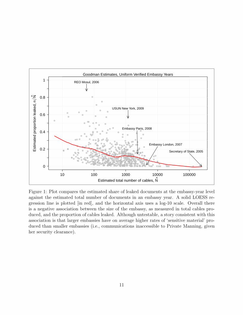
From studying the right-most columns of the table, we see that there is a fair degree of
variation in terms of leaking: the mean proportion leaked is around 13%, but for some
embassy-years it is much larger or smaller. Recalling that there are no ‘Top Secret’ cables
in our data, one explanation for this variation is that documents at that classification level
are not evenly distributed over embassy-years (literally, some embassies send more high level
material at certain times than others). Consequently, regardless of the N estimated for the
embassy-year in question, the numerator in the proportion calculation is lower in some cases
than others. Figure 1 plots the proportion leaked for all embassy-years in this sample, with
some ‘interesting’ cases highlighted.
9
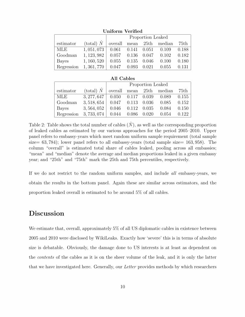
Uniform VerifiedProportion Leaked
estimator (total) N overall mean 25th median 75thMLE 1, 051, 073 0.061 0.141 0.051 0.109 0.188Goodman 1, 123, 982 0.057 0.136 0.047 0.102 0.182Bayes 1, 160, 520 0.055 0.135 0.046 0.100 0.180Regression 1, 361, 770 0.047 0.093 0.021 0.055 0.131
All CablesProportion Leaked
estimator (total) N overall mean 25th median 75thMLE 3, 277, 647 0.050 0.117 0.039 0.089 0.155Goodman 3, 518, 654 0.047 0.113 0.036 0.085 0.152Bayes 3, 564, 052 0.046 0.112 0.035 0.084 0.150Regression 3, 733, 074 0.044 0.086 0.020 0.054 0.122
Table 2: Table shows the total number of cables (N), as well as the corresponding proportionof leaked cables as estimated by our various approaches for the period 2005–2010. Upperpanel refers to embassy-years which meet random uniform sample requirement (total samplesize= 63, 784); lower panel refers to all embassy-years (total sample size= 163, 958). Thecolumn “overall” is estimated total share of cables leaked, pooling across all embassies;“mean” and “median” denote the average and median proportions leaked in a given embassyyear; and “25th” and “75th” mark the 25th and 75th percentiles, respectively.
If we do not restrict to the random uniform samples, and include all embassy-years, we
obtain the results in the bottom panel. Again these are similar across estimators, and the
proportion leaked overall is estimated to be around 5% of all cables.
Discussion
We estimate that, overall, approximately 5% of all US diplomatic cables in existence between
2005 and 2010 were disclosed by WikiLeaks. Exactly how ‘severe’ this is in terms of absolute
size is debatable. Obviously, the damage done to US interests is at least as dependent on
the contents of the cables as it is on the sheer volume of the leak, and it is only the latter
that we have investigated here. Generally, our Letter provides methods by which researchers
10
Goodman Estimates, Uniform Verified Embassy Years
Estimated total number of cables, N
Est
imat
ed p
ropo
rtio
n le
aked
, nN
0
0.2
0.4
0.6
0.8
1
10 100 1000 10000 100000
Secretary of State, 2005
REO Mosul, 2006
USUN New York, 2009
Embassy London, 2007
Embassy Paris, 2008
Figure 1: Plot compares the estimated share of leaked documents at the embassy-year levelagainst the estimated total number of documents in an embassy year. A solid LOESS re-gression line is plotted [in red], and the horizontal axis uses a log-10 scale. Overall thereis a negative association between the size of the embassy, as measured in total cables pro-duced, and the proportion of cables leaked. Although untestable, a story consistent with thisassociation is that larger embassies have on average higher rates of ‘sensitive material’ pro-duced than smaller embassies (i.e., communications inaccessible to Private Manning, givenher security clearance).
11

can be aware of the sample size available to them, overall and by embassy-year should they
choose to work with such data. Assuming the official sources (either leaked or declassified)
use numbering conventions as discussed here, the same techniques can be used for other
projects. Future work might consider the content of the cables, and utilize our estimates in
regression-type analyses.
12

Online Appendix A Verifying Samples are Random from
Discrete Uniform
Goodman (1954) suggests several ways to check that a given sample of serial numbers is a
random sample from a discrete uniform distribution. First, denoting g the largest number in
the sample, divide each of the remaining k− 1 observations in the sample by g. These k− 1
observations should then be statistically indistinguishable from a uniform on [0, 1], with a
Kolmogorov-Smirnov test an appropriate way to check this. Second, one may break the data
into equally spaced ordinal categories, and then conduct a χ2-test on this coarsened data:
if the null cannot be rejected, then the data is at least consistent with a discrete uniform.
Both tests are straightforward to implement, and we use the former.
Online Appendix B Power of the Uniformity Tests
The techniques applied in this Letter work optimally when the sample is one drawn from a
discrete uniform distribution of serial numbers. This does not mean that any bias induced
by non-uniformity invalidates the general thrust of the results presented in the Letter, but
for completeness, we analyze this first order concern here.
We verified uniformity with the Komologorov-Smirnov (KS) test noted above, but one may
be concerned as to its power and want to know the circumstances under which that test is
able to correctly reject the null of non-uniformity. While there is a theoretical literature on
the general issue of the power of the KS test (e.g. Durbin, 1961; Lewis, 1965), we wanted
to obtain specific results for our data. Thus we set up a series of simulation experiments in
which we allowed discrete serial numbers to be generated from a set of Beta distributions
(including the uniform as a special case) and considered the performance of the KS test
13
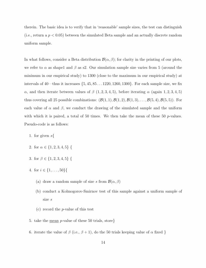
therein. The basic idea is to verify that in ‘reasonable’ sample sizes, the test can distinguish
(i.e., return a p < 0.05) between the simulated Beta sample and an actually discrete random
uniform sample.
In what follows, consider a Beta distribution B(α, β); for clarity in the printing of our plots,
we refer to α as shape1 and β as s2. Our simulation sample size varies from 5 (around the
minimum in our empirical study) to 1300 (close to the maximum in our empirical study) at
intervals of 40—thus it increases {5, 45, 85 . . . 1220, 1260, 1300}. For each sample size, we fix
α, and then iterate between values of β (1, 2, 3, 4, 5), before iterating α (again 1, 2, 3, 4, 5)
thus covering all 25 possible combinations: (B(1, 1),B(1, 2),B(1, 3), . . . ,B(5, 4),B(5, 5)). For
each value of α and β, we conduct the drawing of the simulated sample and the uniform
with which it is paired, a total of 50 times. We then take the mean of these 50 p-values.
Pseudo-code is as follows:
1. for given s{
2. for α ∈ {1, 2, 3, 4, 5} {
3. for β ∈ {1, 2, 3, 4, 5} {
4. for i ∈ {1, . . . , 50}{
(a) draw a random sample of size s from B(α, β)
(b) conduct a Kolmogorov-Smirnov test of this sample against a uniform sample of
size s
(c) record the p-value of this test
5. take the mean p-value of these 50 trials, store}
6. iterate the value of β (i.e., β + 1), do the 50 trials keeping value of α fixed }
14
7. iterate the value of α (i.e., α + 1), iterate through values of β for that value of α }
8. iterate the size of the sample to the next entry in the sample size vector }
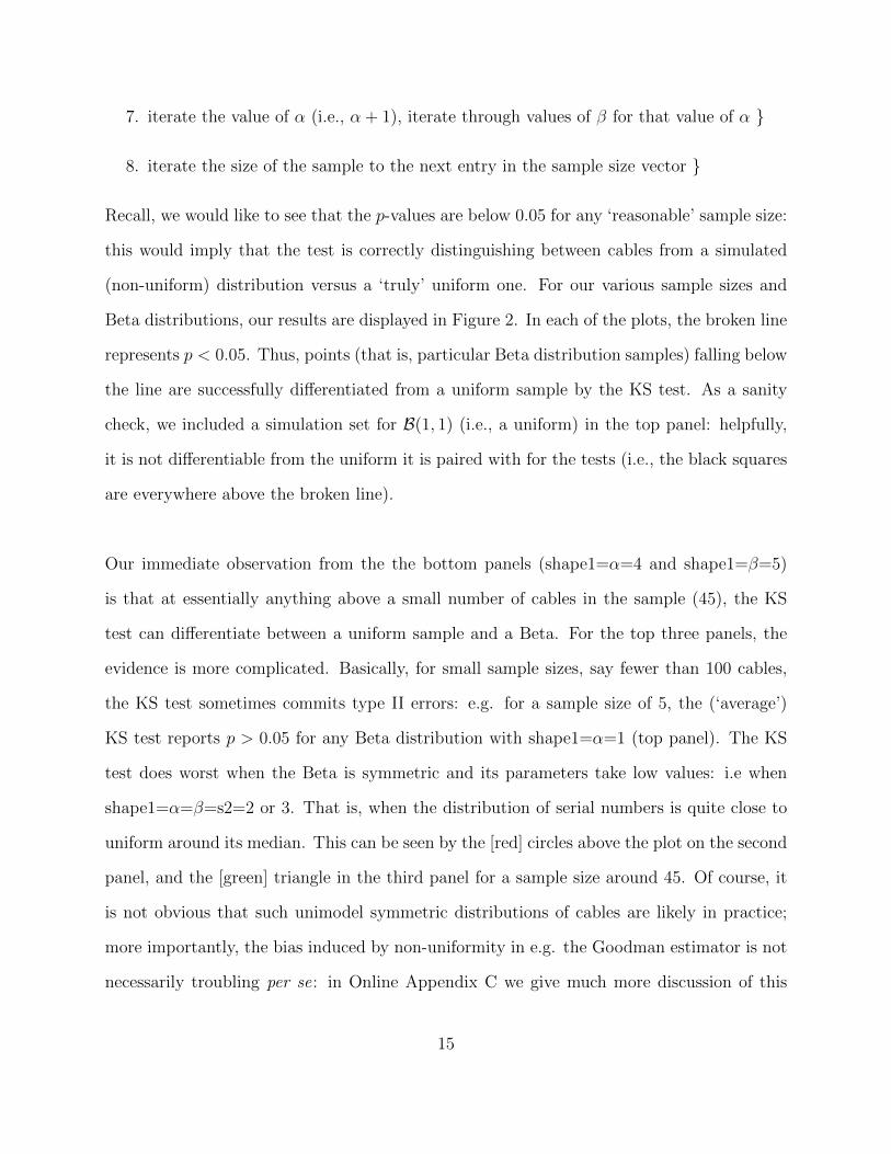
Recall, we would like to see that the p-values are below 0.05 for any ‘reasonable’ sample size:
this would imply that the test is correctly distinguishing between cables from a simulated
(non-uniform) distribution versus a ‘truly’ uniform one. For our various sample sizes and
Beta distributions, our results are displayed in Figure 2. In each of the plots, the broken line
represents p < 0.05. Thus, points (that is, particular Beta distribution samples) falling below
the line are successfully differentiated from a uniform sample by the KS test. As a sanity
check, we included a simulation set for B(1, 1) (i.e., a uniform) in the top panel: helpfully,
it is not differentiable from the uniform it is paired with for the tests (i.e., the black squares
are everywhere above the broken line).
Our immediate observation from the the bottom panels (shape1=α=4 and shape1=β=5)
is that at essentially anything above a small number of cables in the sample (45), the KS
test can differentiate between a uniform sample and a Beta. For the top three panels, the
evidence is more complicated. Basically, for small sample sizes, say fewer than 100 cables,
the KS test sometimes commits type II errors: e.g. for a sample size of 5, the (‘average’)
KS test reports p > 0.05 for any Beta distribution with shape1=α=1 (top panel). The KS
test does worst when the Beta is symmetric and its parameters take low values: i.e when
shape1=α=β=s2=2 or 3. That is, when the distribution of serial numbers is quite close to
uniform around its median. This can be seen by the [red] circles above the plot on the second
panel, and the [green] triangle in the third panel for a sample size around 45. Of course, it
is not obvious that such unimodel symmetric distributions of cables are likely in practice;
more importantly, the bias induced by non-uniformity in e.g. the Goodman estimator is not
necessarily troubling per se: in Online Appendix C we give much more discussion of this
15

(potential) issue. Finally, notice that when we get up to our mean sample size (around 100)
the KS test generally gets it right and has the power we need, with the exception of the
case where α = β = 2 and we need a sample size of around 300 to be confident we have a
uniform.
Online Appendix C Simulation Study
We assume the sample of cable serial numbers observed in each embassy year to be draws
from a discrete uniform distribution, in keeping with the practice in Goodman (1952) and
Goodman (1954) and other studies. In the context of our applied research question, the
discrete uniformity assumption means that each serial number, within a given embassy year,
has the same ex ante probability of being included in the final Manning sample.
In this appendix, we briefly discuss conditions under which the discrete uniformity assump-
tion is appropriate to estimate the cable population size for all cables originating from a
particular embassy in a given year, and how the Goodman estimator tends to perform in
settings where discrete uniformity is violated. To perform these analyses, we simulate cables
being written at the daily level (and being released over the course of a year) and observe
how non-constant probabilities of cables arriving in the final Manning sample may bias es-
timates of cable population sizes. In brief, we find that temporal shifts in the probability
cables are excluded from the Manning sample are more likely to bias estimates of the total
population size than vicissitudes in the daily rate of cables being written.
We close this document with a replication of our serial number analysis using a regression-
based approach that incorporates information on the timing of each cable observed in the
sample to help inform our estimates of the cable population size in each embassy-year. In
16
020
040
060
080
010
0012
000.00.40.8
p value
shap
e1=1
●
●●
●●
●●
●●
●●
●●
●●
●●
●●
●●
●●
●●
●●
●●
●●
●●
●
●●
●●
●●
●●
●●
●●
●●
●●
●●
●●
●●
●●
●●
●●
●●
●●
● ●
s2=
1s2
= 2
s2=
3s2
= 4
s2=
5
020
040
060
080
010
0012
00
0.00.40.8
p value
shap
e1=2
●
●
●●
●●
●●
●●
●●
●●
●●
●●
●●
●●
●●
●●
●●
●●
●●
●
●
●●
●●
●●
●●
●●
●●
●●
●●
●●
●●
●●
●●
●●
●●
●●
●●
● ●
s2=
1s2
= 2
s2=
3s2
= 4
s2=
5
020
040
060
080
010
0012
00
0.00.40.8
p value
shap
e1=3
●
●●
●●
●●
●●
●●
●●
●●
●●
●●
●●
●●
●●
●●
●●
●●
●●
●
●
●●
●●
●●
●●
●●
●●
●●
●●
●●
●●
●●
●●
●●
●●
●●
●
● ●
s2=
1s2
= 2
s2=
3s2
= 4
s2=
5
020
040
060
080
010
0012
00
0.00.40.8
p value
shap
e1=4
●
●●
●●
●●
●●
●●
●●
●●
●●
●●
●●
●●
●●
●●
●●
●●
●●
●
●●
●●
●●
●●
●●
●●
●●
●●
●●
●●
●●
●●
●●
●●
●●
●●
● ●
s2=
1s2
= 2
s2=
3s2
= 4
s2=
5
0.00.40.8
p value
shap
e1=5
●
●●
●●
●●
●●
●●
●●
●●
●●
●●
●●
●●
●●
●●
●●
●●
●●
●
●●
●●
●●
●●
●●
●●
●●
●●
●●
●●
●●
●●
●●
●●
●●
●●
● ●
s2=
1s2
= 2
s2=
3s2
= 4
s2=
5
Fig
ure
2:P
ower
ofth
eK
olm
ogor
ov-S
mir
nov
test
(lit
eral
ly,y-a
xis
isa
mea
np-
valu
e)fo
rva
riou
sva
lues
ofa
Bet
adis
trib
uti
onve
rsus
aunif
orm
,at
vari
ous
sam
ple
size
s(x
-axis
).T
opplo
tfixes
firs
tB
eta
par
amet
erat
1(‘
shap
e1=
1’),
vari
esth
ese
cond
(s2;
see
lege
nd).
Sec
ond
plo
tfixes
firs
tB
eta
par
amet
erat
2,va
ries
the
seco
nd.
Thir
dplo
tfixes
firs
tB
eta
par
amet
erat
3an
dso
on.
Bro
ken
line
repre
sentsp
=0.
05,
and
thus
all
poi
nts
bel
owth
isline
are
succ
essf
ully
dis
tingu
ished
from
the
unif
orm
by
the
KS
test
.
17
general, when the discrete uniformity assumption is satisfied, both Goodman-type estimates
and regression-based approaches provide unbiased estimates of the population size; under
some conditions, however, regression-based techniques may be preferable to the Goodman
estimator if there are sharp changes in the probability is excluded from the Manning sample
near the end of a calendar year, or if reasonable assumptions can be made about a fixed
expected rate of cable generation across periods.
C.1 Overview
Our objective is to observe how various population size estimators perform on simulated
data when (a) there may be seasonality in the rate at which cables are written, (b) there
may exist seasonality in the sensitivity of cables being written. We also seek to inspect how
such biases may manifest in large versus small sample settings. Evaluating such concerns
through simulations, however, will require our making somewhat stylized assumptions about
the data generation process of our sample. The main conclusions of our simulation studies
are as follows: large shifts in the probability cables are excluded from the Manning sample
are more likely to bias Goodman-type estimates of population size than shifts in the number
of cables created per day. For the Goodman estimator, the bias introduced is greater as the
probability of inclusion in the Manning sample is decreasing over time.
To reach these conclusions, in first set of simulations, we will assume the number of ca-
bles written on a particular day is a draw from a Poisson distribution with a fixed rate
parameter. In a second set, we model the number of cables written per day as realizations of
a Hawkes process (e.g., Hawkes, 1971; Ogata, 1988), which allows the instantaneous rate of
cable generation to vary as a part of a “self-exciting” point process, where the occurrence of
any event (i.e., a cable being written) increases the short term probability of another cable
being written. In our applied context, the simulated Hawkes process will lead to clustered
18
periods of time with higher than baseline (i.e., random) patterns of cable generation. For
one set of Poisson simulations, we will set the rate parameter to equal λ = 5. For one set
of Hawkes simulations, we will set the initial conditions to equal µ = 10/3, α1 = 1, and
β1 = 3, and simulate events in continuous time for T = 365. These parameters were selected
because they generate, in expectation, equal totals of cables over the course of an entire
year, but vary in terms of their temporal clustering and variance.8 The virtue in maintain-
ing approximately equal yearly sample sizes in the Poisson and Hawkes study conditions is
that it allows for easy inspection of how clustered periods of higher cable generation rates—
rather than sample size on its own, or variation in the probability serial numbers are out of
sample—influence population size estimates.9 As the next section will show, however, the
‘burstiness’ of cables being generated over time may be more likely to bias regression-based
estimates of population size when such periods of time are correlated with large shifts in the
probability cables are excluded from the Manning sample. Goodman-type estimators (which
rely more heavily on the observed value of the sample maximum serial number) may be less
sensitive to burst-induced biases if the probability that cables appear in the Manning sample
is sufficiently high near the end of a calendar year.
C.2 Sensitivity of Assumptions for Goodman and Regression-based
Estimators
Absent large shifts over time in the probability that serial numbers are excluded from the
Manning sample, daily cable counts being produced from Poisson and Hawkes processes are
8In addition to the “Large N” case where the expected number of cables written per year is 1825, we willalso replicate our analysis on a “Small N” case when the expected yearly total is 365.
9If the number of cables created on any given day is nt ∼ Pois(λ), then the expected number of cables
being created over the course of a year is simply∑365t=1E[nt] = 365 · 5 = 1825. In a Hawkes process, the
instantaneous rate parameter in time t is λ(t) = µ+∑ti<t
αeβ(t−ti). Under the condition that the exponentialrate of decay is greater than the self-excitation growth rate (β > α), and as the number of periods T →∞,the expected value of the rate parameter is E[λ] = µ
1−∫∞0αe−βtdt
= µ1−(α/β) .
19
both acceptable for the Goodman and regression-based estimators of cable population size
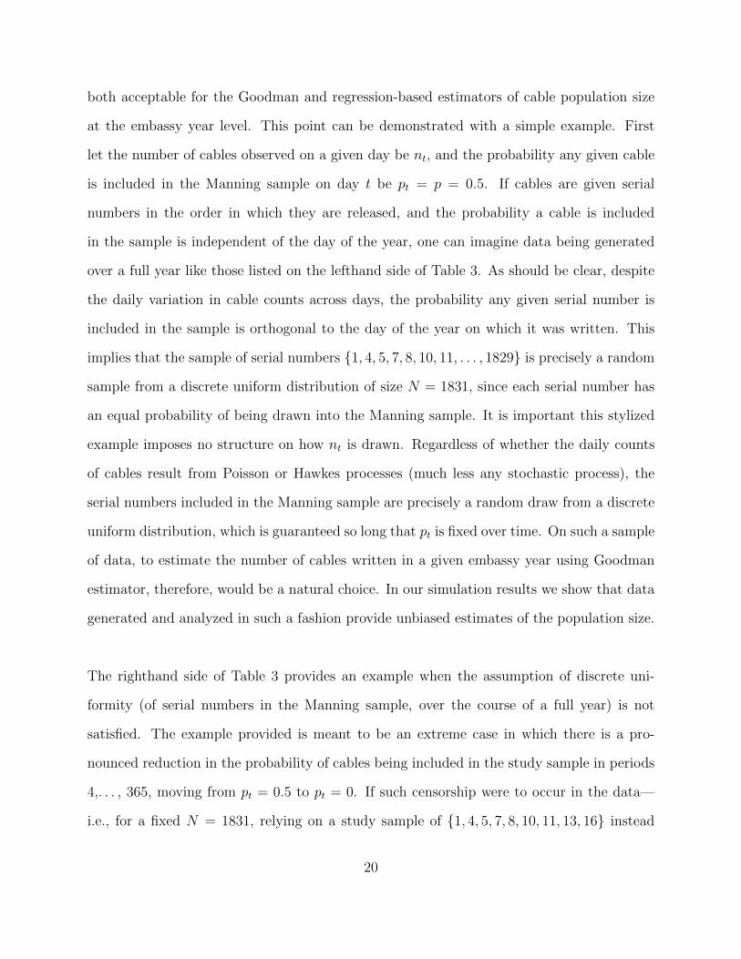
at the embassy year level. This point can be demonstrated with a simple example. First
let the number of cables observed on a given day be nt, and the probability any given cable
is included in the Manning sample on day t be pt = p = 0.5. If cables are given serial
numbers in the order in which they are released, and the probability a cable is included
in the sample is independent of the day of the year, one can imagine data being generated
over a full year like those listed on the lefthand side of Table 3. As should be clear, despite
the daily variation in cable counts across days, the probability any given serial number is
included in the sample is orthogonal to the day of the year on which it was written. This
implies that the sample of serial numbers {1, 4, 5, 7, 8, 10, 11, . . . , 1829} is precisely a random
sample from a discrete uniform distribution of size N = 1831, since each serial number has
an equal probability of being drawn into the Manning sample. It is important this stylized
example imposes no structure on how nt is drawn. Regardless of whether the daily counts
of cables result from Poisson or Hawkes processes (much less any stochastic process), the
serial numbers included in the Manning sample are precisely a random draw from a discrete
uniform distribution, which is guaranteed so long that pt is fixed over time. On such a sample
of data, to estimate the number of cables written in a given embassy year using Goodman
estimator, therefore, would be a natural choice. In our simulation results we show that data
generated and analyzed in such a fashion provide unbiased estimates of the population size.
The righthand side of Table 3 provides an example when the assumption of discrete uni-
formity (of serial numbers in the Manning sample, over the course of a full year) is not
satisfied. The example provided is meant to be an extreme case in which there is a pro-
nounced reduction in the probability of cables being included in the study sample in periods
4,. . . , 365, moving from pt = 0.5 to pt = 0. If such censorship were to occur in the data—
i.e., for a fixed N = 1831, relying on a study sample of {1, 4, 5, 7, 8, 10, 11, 13, 16} instead
20
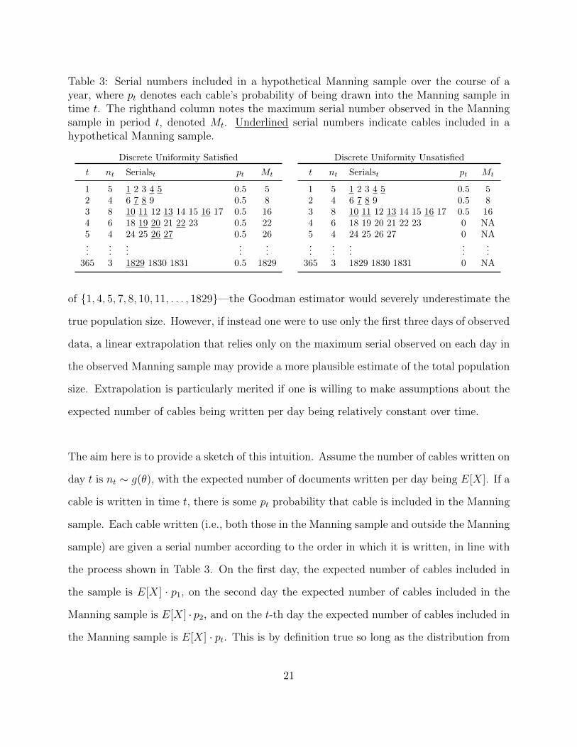
Table 3: Serial numbers included in a hypothetical Manning sample over the course of ayear, where pt denotes each cable’s probability of being drawn into the Manning sample intime t. The righthand column notes the maximum serial number observed in the Manningsample in period t, denoted Mt. Underlined serial numbers indicate cables included in ahypothetical Manning sample.
Discrete Uniformity Satisfied
t nt Serialst pt Mt
1 5 1 2 3 4 5 0.5 52 4 6 7 8 9 0.5 83 8 10 11 12 13 14 15 16 17 0.5 164 6 18 19 20 21 22 23 0.5 225 4 24 25 26 27 0.5 26...
......
......
365 3 1829 1830 1831 0.5 1829
Discrete Uniformity Unsatisfied
t nt Serialst pt Mt
1 5 1 2 3 4 5 0.5 52 4 6 7 8 9 0.5 83 8 10 11 12 13 14 15 16 17 0.5 164 6 18 19 20 21 22 23 0 NA5 4 24 25 26 27 0 NA...
......
......
365 3 1829 1830 1831 0 NA
of {1, 4, 5, 7, 8, 10, 11, . . . , 1829}—the Goodman estimator would severely underestimate the
true population size. However, if instead one were to use only the first three days of observed
data, a linear extrapolation that relies only on the maximum serial observed on each day in
the observed Manning sample may provide a more plausible estimate of the total population
size. Extrapolation is particularly merited if one is willing to make assumptions about the
expected number of cables being written per day being relatively constant over time.
The aim here is to provide a sketch of this intuition. Assume the number of cables written on
day t is nt ∼ g(θ), with the expected number of documents written per day being E[X]. If a
cable is written in time t, there is some pt probability that cable is included in the Manning
sample. Each cable written (i.e., both those in the Manning sample and outside the Manning
sample) are given a serial number according to the order in which it is written, in line with
the process shown in Table 3. On the first day, the expected number of cables included in
the sample is E[X] · p1, on the second day the expected number of cables included in the
Manning sample is E[X] · p2, and on the t-th day the expected number of cables included in
the Manning sample is E[X] · pt. This is by definition true so long as the distribution from
21
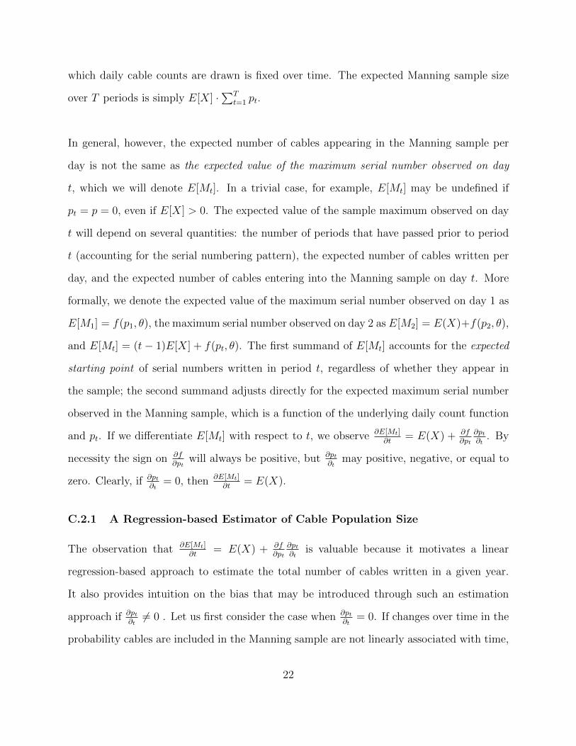
which daily cable counts are drawn is fixed over time. The expected Manning sample size
over T periods is simply E[X] ·∑T
t=1 pt.
In general, however, the expected number of cables appearing in the Manning sample per
day is not the same as the expected value of the maximum serial number observed on day
t, which we will denote E[Mt]. In a trivial case, for example, E[Mt] may be undefined if
pt = p = 0, even if E[X] > 0. The expected value of the sample maximum observed on day
t will depend on several quantities: the number of periods that have passed prior to period
t (accounting for the serial numbering pattern), the expected number of cables written per
day, and the expected number of cables entering into the Manning sample on day t. More
formally, we denote the expected value of the maximum serial number observed on day 1 as
E[M1] = f(p1, θ), the maximum serial number observed on day 2 as E[M2] = E(X)+f(p2, θ),
and E[Mt] = (t− 1)E[X] + f(pt, θ). The first summand of E[Mt] accounts for the expected
starting point of serial numbers written in period t, regardless of whether they appear in
the sample; the second summand adjusts directly for the expected maximum serial number
observed in the Manning sample, which is a function of the underlying daily count function
and pt. If we differentiate E[Mt] with respect to t, we observe ∂E[Mt]∂t
= E(X) + ∂f∂pt
∂pt∂t
. By
necessity the sign on ∂f∂pt
will always be positive, but ∂pt∂t
may positive, negative, or equal to
zero. Clearly, if ∂pt∂t
= 0, then ∂E[Mt]∂t
= E(X).
C.2.1 A Regression-based Estimator of Cable Population Size
The observation that ∂E[Mt]∂t
= E(X) + ∂f∂pt
∂pt∂t
is valuable because it motivates a linear
regression-based approach to estimate the total number of cables written in a given year.
It also provides intuition on the bias that may be introduced through such an estimation
approach if ∂pt∂t6= 0 . Let us first consider the case when ∂pt
∂t= 0. If changes over time in the
probability cables are included in the Manning sample are not linearly associated with time,
22
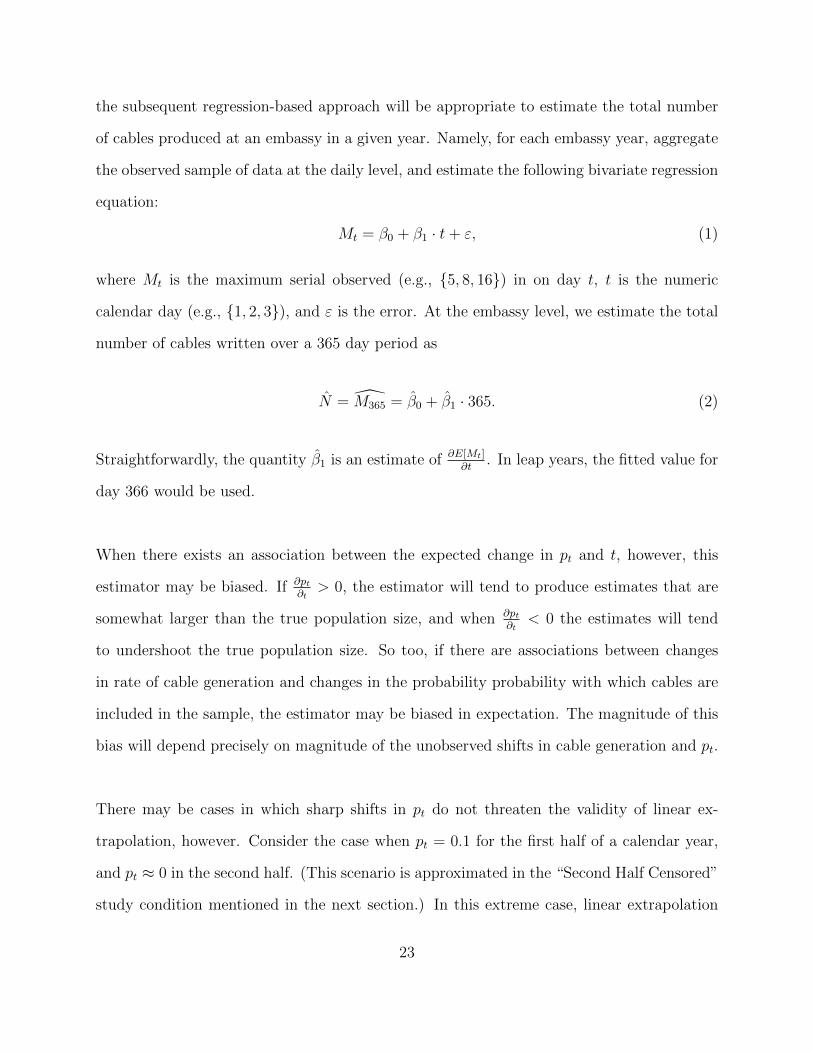
the subsequent regression-based approach will be appropriate to estimate the total number
of cables produced at an embassy in a given year. Namely, for each embassy year, aggregate
the observed sample of data at the daily level, and estimate the following bivariate regression
equation:
Mt = β0 + β1 · t+ ε, (1)
where Mt is the maximum serial observed (e.g., {5, 8, 16}) in on day t, t is the numeric
calendar day (e.g., {1, 2, 3}), and ε is the error. At the embassy level, we estimate the total
number of cables written over a 365 day period as
N = M365 = β0 + β1 · 365. (2)
Straightforwardly, the quantity β1 is an estimate of ∂E[Mt]∂t
. In leap years, the fitted value for
day 366 would be used.
When there exists an association between the expected change in pt and t, however, this
estimator may be biased. If ∂pt∂t
> 0, the estimator will tend to produce estimates that are
somewhat larger than the true population size, and when ∂pt∂t
< 0 the estimates will tend
to undershoot the true population size. So too, if there are associations between changes
in rate of cable generation and changes in the probability probability with which cables are
included in the sample, the estimator may be biased in expectation. The magnitude of this
bias will depend precisely on magnitude of the unobserved shifts in cable generation and pt.
There may be cases in which sharp shifts in pt do not threaten the validity of linear ex-
trapolation, however. Consider the case when pt = 0.1 for the first half of a calendar year,
and pt ≈ 0 in the second half. (This scenario is approximated in the “Second Half Censored”
study condition mentioned in the next section.) In this extreme case, linear extrapolation
23
given the observed data may be reasonable: even though the range of the observed data is
weighted exclusively to the first half of a calendar year, if the true rate of cable generation in
the first half of the year is close to the rate of cable generation in the second half of the year,
the estimates ∂E[Mt]∂t
obtained from the first half of the calendar year should appropriately
map to the second half of the year, even if no data are observed in sample from that period.
C.2.2 Study Conditions and Outcomes of Interest
To assess how various estimators perform across various hypothetical data generation pro-
cesses, we vary both the distribution from which daily cable counts are drawn, in addition
to the probability that any cable written on day t is to be included in the Manning sample.
As before, we denote the probability that a cable is included in the Manning sample, given
that it is written on day t, as pt.
We report simulation results for eight different manipulations of pt. The names of these
study conditions are presented along with their formal definitions in Table 4.
Table 4: Study Manipulations: Variation in the Probability of a Cable’s Inclusion in theManning Sample, given that it was written on day t
Condition Definition
Fixed Probabilities pt = p = 0.1First Half Censored pt = 0.001, if t < 183; pt = 0.1, if t ≥ 183Second Half Censored pt = 0.1, if t < 183; pt = 0.001, if t ≥ 183Random Uniform pt ∼ Unif(0, 0.1)Inverted U-Shape pt = sin(t · π/365)/10U-Shape pt = (1− sin(t · π/365))/10Linear Increase pt = (t/365)/10Linear Decrease pt = (1− t/365)/10
In addition to varying the probability with with written cables appear in the Manning
sample, we vary whether daily cables counts arise as a result of a Poisson process or a Hawkes
process. For both the Poisson and the Hawkes study conditions, we have “Large N” and a
24
“Small N” variants. In the “Large N” conditions, the Poisson parameter is λ = 5, while the
respective Hawkes parameters are defined as µ = 10/3 (the baseline rate), α = 1 (the exci-
tation parameter), and β = 3 (the exponential decay). In the “Small N” study conditions,
the Poisson parameter λ = 1, and the Hawkes parameters are µ = 0.2, α = 0.8, and β = 1.
Using Poisson and Hawkes data generation process, across both the “Large N” and “Small
N” study conditions, we perform 2,500 random simulations of each of the study conditions
listed in Table 4. In each of these simulations we record the “true” number of cables gener-
ated by either the Poisson or Hawkes processes, in addition to the estimates of each of the
MLE, Goodman, and regression-based estimators. In each iteration of the simulation, we
divide each estimator’s estimate of the total population size by the true number, yielding
N/N , and we store this value. If across multiple simulations a particular estimator sys-
tematically yields values of N/N > 1, this provides evidence that an estimator tends to
overestimate the true number of cables. Similarly, if a particular estimator on average yields
values of N/N < 1, this provides evidence that an estimator, given the study conditions,
tends to underestimate the true number of cables in a given embassy year.
C.3 Results
Figures 3 through 6 present the results of this simulation study. In each subplot, the mean
value of N/N across simulations is presented beneath each estimator’s name. The upper
and lower boundaries of each boxplot denote the interquartile range of simulation results for
each estimator. The median result is presented as a solid, horizontal line. The upper and
lower whiskers denote values 1.5 above or below the interquartile range of the plot.
Overall, the regression-based estimator performs consistently well. When the discrete uni-
formity assumption is satisfied, however, the Goodman estimator is unbiased and exhibits
25

the lowest variance. The bias and variance of each estimator appears to be larger in the
“Small N” study conditions. In our applied example, the Goodman estimator is most biased
cases in which pt is decreasing over time. Relative to the “Inverted U-Shape”, the ”U-Shape”
study conditions have distributions of N/N closer to 1.
26
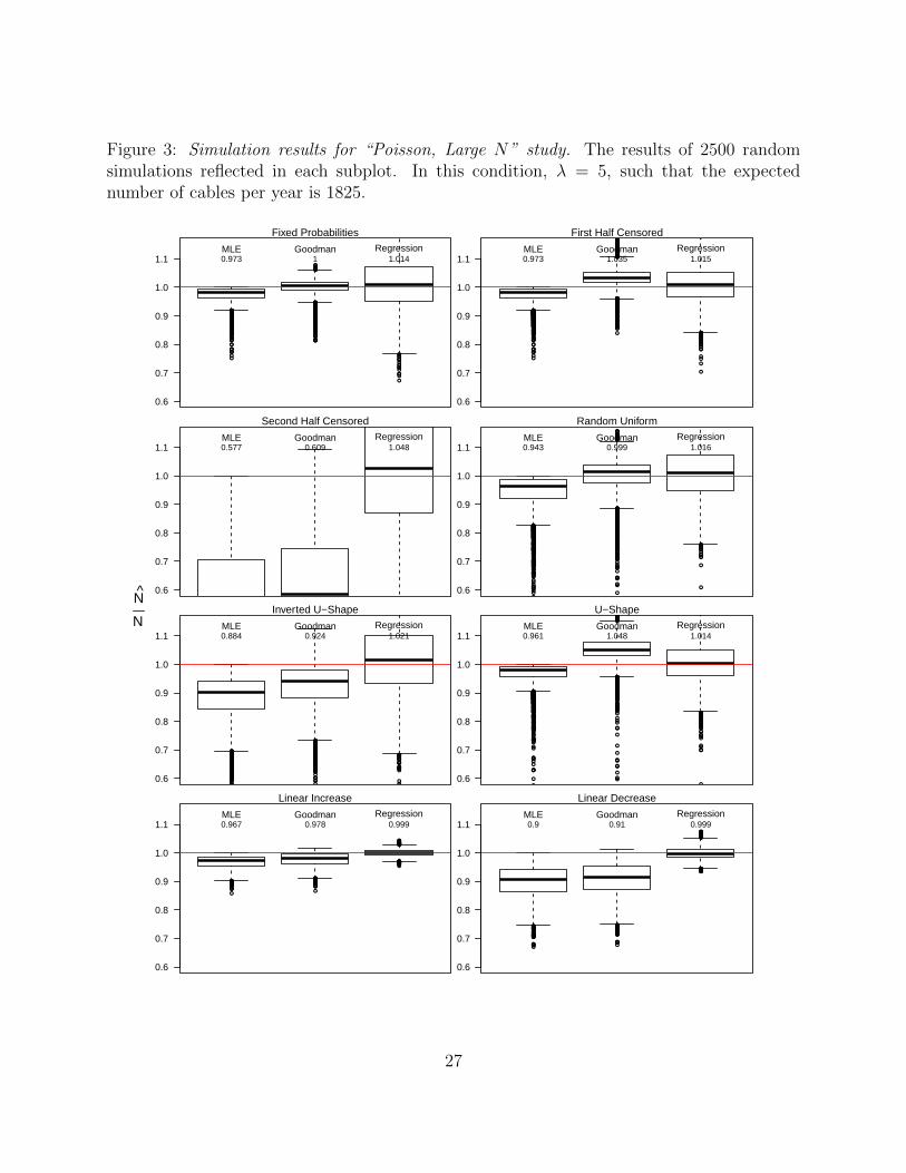
Figure 3: Simulation results for “Poisson, Large N” study. The results of 2500 randomsimulations reflected in each subplot. In this condition, λ = 5, such that the expectednumber of cables per year is 1825.
●
●
●
●
●
●
●●
●
●
●
●
●●
●
●
●
●
●
●
●●●●●
●
●
●
●●●●●●●●●●●
●●●
●●●●●●
●
●
●
●●●
●●●
●
●●●
●
●
●
●●●●
●
●●●
●●●
●●
●
●
●
●●●●●●●●●●
●
●
●●
●
●●
●
●●
●
●
●
●●
●●●●●
●
●
●
●
●●
●●
●
●●
●
●●
●
●
●
●●●●●●
●
●●
●
●
●
●
●
●●●
●
●
●●
●
●
●
●●
●
●
●
●
●●●
●
●●
●●●
●●
●
●
●
●●
●
●●●●●
●
●
●
●
●●
●
●
●
●●●●●
●●
●
●
●●●
●
●
●●●●
●
●●●●
●
●
●
●
●
●
●
●
●●
●●●
●
●
●
●
●
●
●●
●
●
●
●
●
●●●
●●●
●●
●●●●
●
●
●
●●●●●●●●●
●
●
●
●
●●
●
●
●
●
●
●
●●
●●●
●
●
●●●●●●
●
●●●●
●
●
●
●
●
●
●●●●●
●
●
●
●
●●●●●●●●●●
●●●●●●●
●
●
●●
●
●●
●
●●●●
●
●
●●
●
●●
●●
●
●●
●●
●
●●
●
●●●
●●●●●●●●●
●
●
●
●
●
●
●
●
●●
●
●
●
●●
●●
●●●●●
●
●
●
●
●
●
●
●
●●
●
●●
●
●●
●
●●
●
●
●
●●
●
●
●●●
●
●
●●●
●
●
●●
●
●●
●●
●
●
●
●●●
●
●
●●
●
●
●
●●
●
●
●
●
●
●●●●●●
●
●
●
●
●
●
●
●
●
●
●
●
●●
●●
●
●
●●●
●
●●●●●●
●
●
●
●
●
●●
●
●
●●●●
●●
●●
●
●
●
●
●
●
●
●
●
●
●●
●
●●●●●●
●
●●
●●●●
●
●
●
●
●
●●
●
●●●●●
●
●
●
●
●●
●
●
●
●
●
●
●
●
●●●
●●●
●●●
●●
●
●
●
●
●
●●●●
0.6
0.7
0.8
0.9
1.0
1.1MLE Goodman Regression
Fixed Probabilities
0.973 1 1.014
●
●
●
●
●
●
●●
●
●
●
●
●●
●
●
●
●
●
●
●●●●●
●
●
●
●●●●●●●●●●●
●●●
●●●●●●
●
●
●
●●●
●●●
●
●●●
●
●
●
●●●●
●
●●●
●●●
●●
●
●
●
●●●●●●●●●●
●
●
●●
●
●●
●
●●
●
●
●
●●
●●●●●
●
●
●
●
●●
●●
●
●●
●
●●
●
●
●
●●●●●●
●
●●
●
●
●
●
●
●●●
●
●
●●
●
●
●
●●
●
●
●
●
●●●
●
●●
●●●
●●
●
●
●
●●
●
●●●●●
●
●
●
●
●●
●
●
●
●●●●●
●●
●
●
●●●
●
●
●●●●
●
●●●●
●
●
●
●
●
●
●
●
●●
●●●
●
●
●
●
●
●
●●
●
●
●
●
●
●●●
●●●
●●
●●●●
●
●
●
●●●●●●●●●
●
●
●
●
●●
●
●
●
●
●
●
●●
●●●
●
●
●●
●
●●
●
●
●
●
●
●
●●
●
●●●
●
●
●
●
●●
●●●
●●
●
●
●
●
●
●
●
●●
●●
●●●
●
●
●
●
●
●
●
●
●
●
●
●●
●
●
●
●
●
●
●
●
●
●
●●
●
●
●
●●
●
●●●
●
●
●●●
●
●
●●
●
●
●●
●●●
●
●●●
●
●
●●
●
●●
●
●
●
●●
●
●
●
●
●
●
●
●
●
●
●
●
●
●
●
●●
●
●
●●●
●
●
●●
●
●
●
●
●●●
●
●
●
●●●
●
●
●
●●
●
●●
●●●
●
●
●
●
●
●●
●
●
●●
●
●●
●●
●
●
●
●
●
●
●
●
●●
●●
●●
●
●●
●●
●
●
●●●
●●●●
●●
●
●
●
●
●
●
●
●
●
●
●
●
●
●
●
●
●
●
●
●
●●
●
●
●
●
●
●
●
●●●●
●
●
●
●●●●
●
●
●
●
●●
●
●
●●
●●
●●
●
●
●
●●
●
●
●
●
●
●
●
●
●
●
●
●
●●
●
●
●●
●
●
●●
●
●
●
●
●
●
●
●
●
●
●
●
●
●●●
●●
●
●
●
●
●
●
●●
●
●
●
●
●●
●
●
●
●
●
●
●●
●
●
●
●
●●●
●
●
●●●
●
●
●
●●
●
●
●
●
●
●
●
●
●
●
●
●
●
●
●
●
●
●
●●
●
●
●
●
●
●●
●
●
●
●
●●●
●
●
●
●●
●
●
●
●
●
●●
●
●●
●
●
●
●
●
●
●
●●
●●
●
●
●
●
●
●●
●
●
●
●
●
●
●
●
●●●
●
●
●
●
●
●
●
●
●●
●
●
●●
●
●
●
●●
●
●
●●
●
●
●●●
●●●
●●
●
●●
●●●●
0.6
0.7
0.8
0.9
1.0
1.1MLE Goodman Regression
First Half Censored
0.973 1.035 1.015
●
●
●
●
●●
●
●
●
●●
●●
●
●
●
●
●
●
●
●
●
●
●
●
●
●
●
●
●
●
●●
●●
●●
●
●
●
●
●
●
●
●
●
●
●
●
●●
●●
●●
●
●●
●
●
●●
●●●
●●●
●
●
●
●●
●●
●
●
●
●
●
●
●
●
●
0.6
0.7
0.8
0.9
1.0
1.1MLE Goodman Regression
Second Half Censored
0.577 0.609 1.048
●
●
●
●
●●
●●●
●
●
●
●
●
●
●
●
●
●●
●
●
●
●●●●
●
●
●
●
●
●
●●●●
●●●
●
●
●
●
●
●
●
●●
●
●
●
●
●
●
●●
●
●●●●
●
●
●
●●
●
●
●
●
●
●
●●
●
●
●
●
●
●
●●
●
●●●
●
●
●●
●
●
●
●
●
●
●
●
●
●
●
●
●
●●●
●
●
●
●
●
●
●
●●
●
●
●
●●●
●●
●
●
●
●
●
●
●●●●
●●●
●
●●
●
●
●●
●
●
●
●
●●
●●
●
●●
●
●
●
●
●
●●
●
●
●
●●
●
●
●
●
●
●
●
●
●
●
●
●
●
●
●
●●
●
●
●
●
●
●
●
●
●
●●
●●
●●●
●
●●●
●
●
●●
●
●●
●●
●●
●●
●●
●
●●●●
●
●
●●
●
●●
●
●
●
●
●
●
●
●
●
●●
●
●
●
●●●
●
●
●
●
●
●
●
●
●
●●
●
●
●
●
●●
●●
●
●
●●
●
●●
●
●
●
●
●
●
●
●
●●
●
●
●
●●
●
●
●
●
●
●
●
●●
●
●
●●
●●
●
●
●
●
●
●
●
●●
●
●
●●
●
●●
●
●
●
●
●
●
●●●
●
●●
●
●
●
●
●
●
●
●
●
●●●
●
●
●
●
●
●
●
●
●
●●●
●●
●
●
●●●
●
●
●
●
●●
●
●
●
●
●
●
●
●
●
●
●
●
●
●
●
●
●●●
●
●●
●
●●
●
●
●
●●
●
●
●
●
●●
●
●
●
●
●
●●
●
●
●
●
●●
●●
●●
●●●
●
●●
●
●●
●
●
●
●
●
●
●
●●●
●
●
●
●
●
●
●
●●
●
●
●●
●
●
●
●
●
●
●
●
●
●
●●●●
●
●
●
●
●
●
●
●
●●
●
●
●●
●
●
●●
●
●
●
●
●●●
●
●
●
●
●
●
●
●
●
●
●
●●
●●
●
●
●
●
●●
●
●
●
●
●●
●●
●
●●
●
●
●
●
●
●
●
●
●
●
●
●
●
●●●
●
●
●
●
●
●
●
●
●
●
●
●
●
●
●
●
●
●
●
●
●
●●●●
●
●
●
●
●
●
●
●
●
●
●●
●
●
●
●
●●
●
●
●
●
●
●
●●
●
●
●
●
●
●
●
●
●
●
●
●
●
●
●
●
●
●
●
●
●
●
●
●
●
●
●
●
●
●
●
●
●●
●
●
●
●
●
●●
●
●
●
●
●
●
●
●
●●
●
●
●
●
●
●
●
●
●
●
●
●
●
●
●
●
●
●
●
●
●
●
0.6
0.7
0.8
0.9
1.0
1.1MLE Goodman Regression
Random Uniform
0.943 0.999 1.016
●●●
●
●
●
●
●
●●
●
●●●
●
●
●●
●
●
●
●●●●●
●
●
●●
●
●
●
●
●
●
●●
●●●
●
●
●
●●●
●
●●●
●
●
●
●
●
●
●●
●
●
●●
●
●
●
●
●
●●
●
●
●
●
●
●
●●
●
●
●
●●
●
●
●
●●●●
●
●
●
●
●
●
●
●
●
●
●
●
●
●
●
●●
●
●
●
●
●●
●
●
●●
●
●
●
●
●
●
●●
●
●●
●
●●
●
●
●
●
●
●
●
●
●
●
●
●
●
●
●●●●●●●
●
●●●
●
●
●
●
●
●
●
●
●
●
●
●
●
●●
●●
●
●
●
●
●
●
●
●
●●●
●
●
●
●
●
●●
●
●
●●
●
●●
●
●
●
●
●●
●
●
●
●
●
●●
●●
●
●
●●●
●
●●
●
●
●
●
●
●
●
●
●
●●●●
●
●
●
●
●
●
●
●
●
●
●
●
●●●
●
●
●
●
●
●
●
●
●
●●●
●
●
●
●
●●
●
●
●●
●
●
●
●●
●
●
●
●
●
●
●
●
●
●●
●●●●
●
●
●
●
●●
●
●●
●
●
●
●●
●●
●
●
●●
●
●
●
●
●
●
●
●●
●●
●
●
●
●
●
●
●
●
●●
●
●
●
●
●
●
●
●
●
●
●
●
●
●
●
●
●
●
●
●●
●
●
●
●
●
●
●
●
●
●
●
●
●
●
●
●
●
●
●
●
●
●
●
0.6
0.7
0.8
0.9
1.0
1.1MLE Goodman Regression
Inverted U−Shape
0.884 0.924 1.021
●
●
●
●●
●
●
●
●
●
●
●
●
●
●
●
●●
●
●
●
●
●
●
●
●
●
●
●
●
●●
●
●
●●
●
●
●
●
●
●
●
●
●
●●
●
●
●
●
●
●
●
●
●●
●
●
●
●●
●
●
●
●
●
●
●
●●●●
●
●
●
●●●●●●
●
●
●
●●
●
●
●
●
●
●●
●
●●●
●
●
●
●
●
●●●●
●
●
●●●
●
●
●
●
●
●
●
●
●
●
●
●
●
●
●
●●●
●
●
●
●
●
●
●
●
●
●
●●
●●
●
●
●
●
●
●
●
●●●
●
●
●
●
●
●
●
●
●
●
●
●
●
●
●
●
●●●
●
●●
●
●
●
●
●
●
●
●
●
●
●
●
●
●
●●
●
●
●
●
●
●
●
●
●
●
●
●
●
●
●
●
●
●
●●●
●
●●
●
●
●
●
●
●
●
●
●
●●●
●
●
●
●
●
●
●●
●
●
●
●
●
●
●●●
●
●
●
●
●
●●
●
●
●
●
●
●●
●
●
●
●
●●
●
●●
●●
●
●●
●●
●
●
●
●
●
●
●
●
●
●
●
●
●
●●●●●
●●
●
●
●
●
●
●
●●
●
●●●
●
●
●
●
●
●
●●
●
●
●●
●
●
●
●
●
●
●●
●
●
●
●●●●●
●
●●
●
●
●
●
●
●
●
●
●
●●●●
●
●
●●●
●●
●
●
●
●
●
●
●
●
●●
●
●
●
●
●
●
●
●
●
●
●
●
●
●
●
●
●
●
●
●
●●
●
●
●
●
●
●
●
●●●
●●
●
●
●
●
●
●
●
●
●
●
●
●
●
●
●
●
●
●
●
●●
●
●
●●
●
●●
●
●
●
●
●
●
●
●
●
●
●
●●●●●
●
●
●
●
●
●
●
●
●
●
●
●●
●
●
●
●
●
●
●
●
●
●
●
●
●●●
●
●
●
●
●
●
●
●
●
●
●●
●
●
●
●
●
●
●
●
●
●
●
●
●
●●
●
●
●
●
●●
●
●
●
●
●
●
●
●
●
●●
●
●
●
●●●
●
●
●
●●
●
●
●
●●
●
●
●●●
●
●
●
●
●
●
●
●
●
●
●
●●
●
●
●
●
●
●
●
●
●
●
●
●
●
●
●
●
●
●●
●
●
●
●
●
●
●
●
●
●
●
●●
●
●
●
●●
●
●
●
●
●
●
●
●
●
●
●
●
●
●
●
●
●
●
●
●
●
●
●
●
●
●
●
●
●
●●●
●
●
●
●
●
●
●
●
●
●
●
●
●
●
●
●●
●
●
●
●
●
●
●
●
●●
●
●
●
●
●
●
●
●
●
●
●
●
●●
●
●
●●
●
●
●
●
●
●
●
●
●
●
●
●
●
●
●
●
●
●
●
●
●
●
●
●
●
●
●
●
●
●
●
●
●
●
●
●
●
●
●
●
●
●
●
●
●
●
●
●
●
●
●
●
●
●
●
●
●
●
●
●●
●
●
●
●
●
●
●
●
●
●
●
●
●
●
●
●
●
●
●
●
●●
●
●
●●
●
●
●
●
●
●
●
●
●
●
●
●
●
●
●
●
●
●
●
●
●
●
●
●
●
●
●
●
●
●●
●
●
●
●
●●
●
●
●
●
●
●
●
●
●
●
●
●
●
●
●
●
●
●
●●
●
●
●
●
●
●
●
●
●
●●
●●
●
●
●
●
●
●
●●
●
●
●
●
●
●
●●
●
●
●
●
●
●●
●
●
●
●
●
●
●
●
●
●
●
●
●
●
●
●
●
●
●●
●
●●
●
●
●
●
●
●
●
●
●
●
●
●
●
●
●
●
●
●
●
●
●●
●
●
●
●
●
●
●
●
●
●
●
●
●
●
●
●
●
●
●
●●
●
●
●
●
●
●●
●
●
●
●
●
●
●
●
●
●
●
●
●
●
●
●
●
●
●
●
●
●
●
●
●●
●
●●
●
●
●
●
●●
●
0.6
0.7
0.8
0.9
1.0
1.1MLE Goodman Regression
U−Shape
0.961 1.048 1.014
●●●●
●
●●●●●●●●●●●●
●
●●●●●●
●●●●●
●●●
●
●
●
●●●●●●●●●●
●
●●●●●●
●●
●●●
●●●●
●●
●
●●●●●●
●●
●
●●●●●●
●
●
●
●
●
●
●
●
●●●
●●
●●●
●●
●●
●●
●
●
●●●
●
●●●
0.6
0.7
0.8
0.9
1.0
1.1MLE Goodman Regression
Linear Increase
0.967 0.978 0.999
●●●
●●●●
●
●
●
●
●
●●
●
●
●●●●●
●
●●
●
●●
●
●
●●
●●●
●●●
●
●
●
●
●
●●
●
●
●●●●●●●
●
●●
●
●
●●
●
●
●
●
●
●●
●
●●●●
●
●●
●
●
●●
●●●●
●
●●●●●
●
●●●
●
●
●●
●●
●
●●●●●●
0.6
0.7
0.8
0.9
1.0
1.1MLE Goodman Regression
Linear Decrease
0.9 0.91 0.999
N
N
27
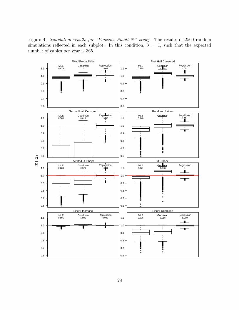
Figure 4: Simulation results for “Poisson, Small N” study. The results of 2500 randomsimulations reflected in each subplot. In this condition, λ = 1, such that the expectednumber of cables per year is 365.
●●●●
●●●
●
●
●●
●
●
●●●●
●
●●●●
●
●
●●
●
●●
●●
●
●●
●
●●●
●
●
●
●●●●
●●
●
●
●
●
●●
●
●●
●●
●●●●●
●●●
●
●●●●●
●
●
●●
●●
●●●●●
●●
●●
●
●
●
●●●●
●
●
●●●●●
●
●
●●
●
●
●
●●●●●●●
●
●●
●●
●
●
●●●●●
●
●
●
●●●
●
●
●●●●
●
●●●
●
●
●●●
●
●
●●●●●●
●
●
●
●●●
●●
●
●
●●
●
●
●●
●
●●
●●
●
●
●●
●
●●
●
●
●
●
●
●●
●
●●●●
●
●●●
●●●
●
●
●
●●
●●●
●●
●
●
●●●
●
●
●
●●
●●
●
●
●
●
●
●
●●●
●●●●●
●
●●
●
●●
●●
●
●●
●●●
●●
●
●
●●●
●●●●
●●
●
●●
●
●●●
●
●●
●
●●●
●
●●●
●
●●
●
●●●●
●
●●
●●●
●
●
●
●
●●●
●
●●
●
●
●●●●●
●●●
●
●●●
●●
●
●
●●●
●●
●●●
●
●●
●●
●●●
●
●
●●●●
●
●●●●●●
●
●
●●
●
●
●
●
●●●●●●
●
●
●●
●
●
●●●●
●
●
●
●
●
●
●
●●
●●●
●
●
●
●●
●
●
●
●
●●●●●●
●
●
●
●●●
●●
●
●
●●
●
●
●●
●
●
●
●●
●
●●
●
●●
●
●
●
●
●
●●●
●
●●●●
●
●●
●●●
●
●
●●
●
●
●
●●●
●●
●
●
●
●●●
●
●●
●
●●
●●●●
●●
●
●●●●●
●
●
●
●●
●
●
●
●
●
●
●
●●
●●
●
●●●●●
●●
●●
●●
●
●●
●●●●●●●
●●
●●●●●●●●
●
●●
●
●●
●
●
●
●●●●
●●
●
●●●
0.6
0.7
0.8
0.9
1.0
1.1MLE Goodman Regression
Fixed Probabilities
0.975 1 1.001
●●●●
●●●
●
●
●●
●
●
●●●●
●
●●●●
●
●
●●
●
●●
●●
●
●●
●
●●●
●
●
●
●●●●
●●
●
●
●
●
●●
●
●●
●●
●●●●●
●●●
●
●●●●●
●
●
●●
●●
●●●●●
●●
●●
●
●
●
●●●●
●
●
●●●●●
●
●
●●
●
●
●
●●●●●●●
●
●●
●●
●
●
●●●●●
●
●
●
●●●
●
●
●●●●
●
●●●
●
●
●●●
●
●
●●●●●●
●
●
●
●●●
●●
●
●
●●
●
●
●●
●
●●
●●
●
●
●●
●
●●
●
●
●
●
●
●●
●
●●●●
●
●●●
●●●
●
●
●
●●
●●●
●●
●
●
●●●
●
●
●
●●
●●
●
●
●
●
●
●
●●●
●●●●●
●
●●
●
●●
●●
●
●●
●●●
●●
●
●
●●
●●
●
●
●
●
●
●
●
●
●●
●
●●
●●
●●
●●●
●
●
●
●
●
●
●
●●
●
●●
●
●
●●●
●
●●
●●
●
●
●●
●●
●
●
●●●●●●●
●
●
●●●●●
●●
●●●●●
●●●
●
●●
●
●●●●
●
●
●
●●
●
●●●●●
●
●
●●●●●
●●●●●●
●
●
●●●
●
●●●
●
●
●●●
●
●
●
●
●
●
●
●●●●
●
●
●●●●
●
●●
●
●●●●
●
●
●
●
●
●●
●
●
●
●
●●
●
●
●
●
●
●
●
●
●
●
●●●
●
●
●
●
●
●
●
●●●●
●
●
●
●
●●
●●●●
●●●●
●
●
●
●
●
●
●
●●●
●
●●●●
●
●●
●●●●●●●
●
●●
●●●●●
●
●
●
●
●●●
●
●●●
●
●
●
●
●●●●
●
●
●
●
●
●●●●
●
●
●
●●
●
●●
●●●●
●
●●
●●●
●●
●
●
●●●●
●
●
●
●●●
●
●●
●
●
●
●●●
●
●●●●●●●●●
●
●●
●●●
●
●●●●
●
●
●
●
●●●●●●●
0.6
0.7
0.8
0.9
1.0
1.1MLE Goodman Regression
First Half Censored
0.975 1.028 1.001
●●
●●
●
●
●
●●
●●
●
●
●
●
●
●●●
●
●
●
●●
●
●
●
●
●
●●●
●
●
●
●
●●●
●
●●
●
●
●
●
●
●●
●
●
●●
●
●●
●
●
●
●●●
●
●
●
●●
●
●
●●
●
●
●
●
●
●
●
●
●
●
●
●
0.6
0.7
0.8
0.9
1.0
1.1MLE Goodman Regression
Second Half Censored
0.589 0.619 1.003
●●
●
●
●●
●
●
●
●
●
●
●
●
●●●
●
●
●
●
●
●●
●
●
●●
●●
●●
●
●●●
●
●●●
●
●
●
●●
●●
●
●●
●
●
●
●
●
●
●
●●
●
●
●
●●●●
●
●
●
●●
●
●●
●
●
●
●
●●
●●
●
●●●
●
●
●●
●
●
●
●●
●
●
●
●
●
●●
●●
●
●
●
●●●
●
●
●
●
●
●●●●
●
●●
●
●
●●
●
●
●●
●
●
●
●●
●●
●●
●
●
●
●
●●
●
●
●●
●●●●
●
●
●●
●
●
●
●
●
●
●●
●
●
●●
●
●
●
●
●
●
●
●
●
●
●
●
●
●
●
●
●●
●●
●
●
●
●
●●
●
●
●●
●
●
●
●
●
●
●
●●
●
●●
●
●
●
●
●●●
●
●
●●
●●●●
●
●
●
●●
●
●
●●
●●
●●
●
●
●
●
●●
●●
●
●●
●
●
●
●●●
●
●
●
●●
●
●●
●
●
●●
●
●
●●
●●●
●
●
●
●●●
●
●
●
●
●●
●
●●
●
●
●
●
●●
●●●
●
●
●
●●●●●
●●
●
●
●●
●
●
●
●
●
●
●
●
●
●●
●
●
●
●
●
●
●●
●
●●
●●
●
●
●
●
●
●●
●
●●
●
●
●
●●●
●●
●●
●
●
●
●
●
●
●●●
●●
●
●
●
●
●
●
●●
●●
●
●
●
●●
●
●
●
●
●
●
●
●
●
●
●
●●
●●
●●●●●
●
●
●●●
●
●
●●●
●
●
●●●●
●
●●●●
●
●
●
●●
●●
●●
●
●●●●
●
●●
●
●
●●
●
●
●
●
●
●
●●●
●
●
●●●
●
●
●
●
●
●●
●
●
●
●●
●●●
●
●
●
●●
●
●●
●●●
●
●
●●
●
●●
●
●●
●
●
●●
●
●●
●
●
●
●
●●●●
●
●●
●
●●
●●●
●
●
●
●●●●
●
●
●
●
●●●●●●●
●●●●
●
●
●●●●
●
●
●
●
●●
●
●●
●
●
●●●
●
●●
●
0.6
0.7
0.8
0.9
1.0
1.1MLE Goodman Regression
Random Uniform
0.948 1 1.001
●
●
●
●
●
●
●●●
●
●
●
●
●●●
●
●
●
●●
●
●
●
●
●
●●
●●
●
●●
●
●
●
●
●
●
●●
●●●
●
●●
●●
●
●●
●
●
●
●●●●
●
●
●
●
●●●●●
●
●
●●
●
●
●
●
●
●●
●●●●●
●●●
●
●
●
●
●
●
●●●
●
●
●●●
●
●●
●●●●
●●
●●
●
●●
●
●
●
●●●●
●
●
●
●●●●
●
●
●
●
●
●
●●●
●●
●●
●
●●
●
●●
●
●●
●
●
●●●
●
●●●●●
●
●
●
●●●●
●●●●
●
●●
●●●
●
●
●●●
●●
●●●
●●
0.6
0.7
0.8
0.9
1.0
1.1MLE Goodman Regression
Inverted U−Shape
0.884 0.921 1.001
●●●●
●
●
●●
●●
●
●●
●●
●●
●
●
●
●
●●●
●
●●
●
●
●
●
●
●
●
●●
●
●
●
●
●●
●
●
●
●●●
●●●
●
●●
●
●
●
●
●
●
●●
●●
●
●
●
●
●●●●
●●●
●
●●
●
●
●●
●
●
●
●
●
●●
●
●
●
●
●
●
●
●
●●
●●
●
●●
●
●
●
●
●
●
●●●
●
●●
●
●
●
●
●●
●●●●●●
●●●
●
●
●
●
●
●●
●●●●
●
●●
●
●
●
●
●
●
●
●
●
●●
●
●
●
●●
●
●
●
●
●●
●
●
●
●
●
●
●
●●●●●
●
●
●
●
●
●
●●●●
●
●
●
●
●
●
●●
●●
●
●
●●
●
●
●
●
●
●
●
●
●
●
●●
●
●●
●●
●
●●
●●
●
●
●
●
●●●
●
●●
●
●●●
●
●●
●
●
●
●
●
●●●
●●
●
●
●
●
●●●●●
●
●
●
●
●
●
●
●
●
●
●
●
●
●
●●
●
●
●
●●
●●
●●
●
●
●
●
●
●
●
●●
●
●
●●
●
●
●
●●●
●
●
●
●
●
●
●
●●●
●●
●
●
●
●
●
●
●●
●
●
●
●
●
●
●
●
●
●
●
●
●
●
●●
●
●
●●●●●
●
●
●
●
●
●
●
●
●
●
●
●
●●●●
●
●
●●●
●●●
●
●●●
●
●
●
●●
●
●
●
●
●
●●
●●
●
●
●
●
●
●
●
●
●
●
●
●
●
●
●●
●
●
●●●
●●
●●
●
●●
●
●●
●
●
●●
●
●●
●
●●●
●
●
●
●
●
●●
●●●
●●
●
●●
●
●●
●●
●
●
●
●
●
●
●●
●
●
●
●
●
●
●
●●
●
●
●●
●
●●●
●
●
●
●
●●
●
●
●
●
●
●●
●
●●●
●
●
●●
●
●
●
●
●
●●
●
●
●
●
●
●
●
●●
●
●●●
●
●
●
●
●
●
●
●
●
●
●
●
●
●
●
●
●
●
●
●
●
●
●
●
●
●
●
●
●
●
●
●●
●
●
●
●●
●
●
●●
●●●
●
●
●
●●●
●
●
●●
●
●
●●
●
●
●
●
●
●
●
●
●
●●
●
●
●●●●
●
●
●●
●
●
●
●
●
●
●
●
●
●
●
●
●●●
●
●
●
●
●
●●
●
●
●
●
●
●●
●●●●●●●
●●
●
●
●
●
●
●
●
●●
●
●●
●
●
●●●●●●
●
●●
●
●
●
●●●●
●●●●●
●
●
●
●
●
●●●
●
●●●●
●
●●
●●
●●●
●●●●●
●●
●●●●
0.6
0.7
0.8
0.9
1.0
1.1MLE Goodman Regression
U−Shape
0.971 1.048 1
●●●●●●●●●●●●●●●●●●●●●●●●●●●●●●●●●
●
●●●●●●●●●●
●
●●●●●●●●●●●●●●●●●●●●●●●●●●●●●●●●●●●●●●●●●●●●●●●●●●●●●●●●●●●
●●●●●●●●●●●●●●●●●●●
●
●●●●●●●●●●●●
●
●●●●●●●●●●●●●●●
●●
●●●●●●●●●●●●●●●●●●●●●●●●●●●●●●●●●●●●●
●
●●●●●●●●
●●●●●●●●●●●●●●●●●●●●●●●●●●●●●●●●●
●●●●●●●●●●●●●●●●●●
●●●●●●●●●●●●●●●●●●●●●●●●●●●●●●●●
●
●●●●●●●●●●
●
●●●●●●●●●●●●●●●●●●●●●●
●●●●●●●●●●●●●●●●●●●●●●●●●●●●●●●●●●
●●●●
●●●●●●●●●●●●●●●●●●●
●●●●●●●●●●●●
●
●●●●●●●●●●●●●●
●
●
●
●●●●●●●●●●●●●●●●●●●●●●●●●●●●●●●●●●●
●
●●●●●●●●●●●●●●●●●●●●●●●●●●●●●●●●●●●●●●●
●
●●●●●●●●●●●●●●●●●●
●●●
●●●●
●
●
●
●
●●
●
●●●●
●
●●●●●
●●●
●
●
●
●
●●●
●
●
●●
●
0.6
0.7
0.8
0.9
1.0
1.1MLE Goodman Regression
Linear Increase
0.995 1.006 0.999
●●●●●●●●
●
●●
●
●
●
●
●●●
●
●
●●
●
●●
●
●
●●●●●●●
●
●
●●
●
●●●●●●●
●
●
●●
●
●
●
●
●
●
●●●
●●●●●
●●
●
●
●
●
●●●
●
●
●●
●
●●
●
●
●●●●●●●●
●
●
●●
●
●●
●●●
●
●
●●
●
●
●
●
●
●
●
●●●
●●●
●●●●●●●●
●●
●
●
●●
●
●
●
●
●
●
●
●
●●
●●●●●
●
●
●●
●
●●
0.6
0.7
0.8
0.9
1.0
1.1MLE Goodman Regression
Linear Decrease
0.906 0.916 0.999
N
N
28
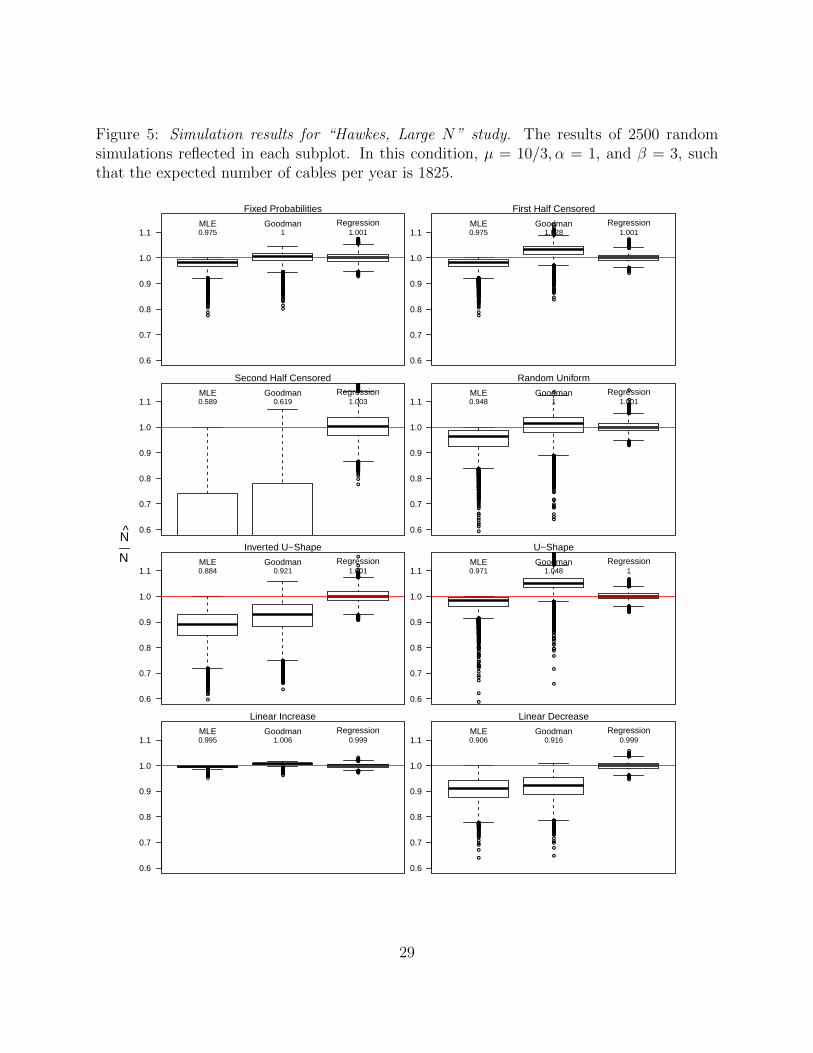
Figure 5: Simulation results for “Hawkes, Large N” study. The results of 2500 randomsimulations reflected in each subplot. In this condition, µ = 10/3, α = 1, and β = 3, suchthat the expected number of cables per year is 1825.
●●●●
●●●
●
●
●●
●
●
●●●●
●
●●●●
●
●
●●
●
●●
●●
●
●●
●
●●●
●
●
●
●●●●
●●
●
●
●
●
●●
●
●●
●●
●●●●●
●●●
●
●●●●●
●
●
●●
●●
●●●●●
●●
●●
●
●
●
●●●●
●
●
●●●●●
●
●
●●
●
●
●
●●●●●●●
●
●●
●●
●
●
●●●●●
●
●
●
●●●
●
●
●●●●
●
●●●
●
●
●●●
●
●
●●●●●●
●
●
●
●●●
●●
●
●
●●
●
●
●●
●
●●
●●
●
●
●●
●
●●
●
●
●
●
●
●●
●
●●●●
●
●●●
●●●
●
●
●
●●
●●●
●●
●
●
●●●
●
●
●
●●
●●
●
●
●
●
●
●
●●●
●●●●●
●
●●
●
●●
●●
●
●●
●●●
●●
●
●
●●●
●●●●
●●
●
●●
●
●●●
●
●●
●
●●●
●
●●●
●
●●
●
●●●●
●
●●
●●●
●
●
●
●
●●●
●
●●
●
●
●●●●●
●●●
●
●●●
●●
●
●
●●●
●●
●●●
●
●●
●●
●●●
●
●
●●●●
●
●●●●●●
●
●
●●
●
●
●
●
●●●●●●
●
●
●●
●
●
●●●●
●
●
●
●
●
●
●
●●
●●●
●
●
●
●●
●
●
●
●
●●●●●●
●
●
●
●●●
●●
●
●
●●
●
●
●●
●
●
●
●●
●
●●
●
●●
●
●
●
●
●
●●●
●
●●●●
●
●●
●●●
●
●
●●
●
●
●
●●●
●●
●
●
●
●●●
●
●●
●
●●
●●●●
●●
●
●●●●●
●
●
●
●●
●
●
●
●
●
●
●
●●
●●
●
●●●●●
●●
●●
●●
●
●●
●●●●●●●
●●
●●●●●●●●
●
●●
●
●●
●
●
●
●●●●
●●
●
●●●
0.6
0.7
0.8
0.9
1.0
1.1MLE Goodman Regression
Fixed Probabilities
0.975 1 1.001
●●●●
●●●
●
●
●●
●
●
●●●●
●
●●●●
●
●
●●
●
●●
●●
●
●●
●
●●●
●
●
●
●●●●
●●
●
●
●
●
●●
●
●●
●●
●●●●●
●●●
●
●●●●●
●
●
●●
●●
●●●●●
●●
●●
●
●
●
●●●●
●
●
●●●●●
●
●
●●
●
●
●
●●●●●●●
●
●●
●●
●
●
●●●●●
●
●
●
●●●
●
●
●●●●
●
●●●
●
●
●●●
●
●
●●●●●●
●
●
●
●●●
●●
●
●
●●
●
●
●●
●
●●
●●
●
●
●●
●
●●
●
●
●
●
●
●●
●
●●●●
●
●●●
●●●
●
●
●
●●
●●●
●●
●
●
●●●
●
●
●
●●
●●
●
●
●
●
●
●
●●●
●●●●●
●
●●
●
●●
●●
●
●●
●●●
●●
●
●
●●
●●
●
●
●
●
●
●
●
●
●●
●
●●
●●
●●
●●●
●
●
●
●
●
●
●
●●
●
●●
●
●
●●●
●
●●
●●
●
●
●●
●●
●
●
●●●●●●●
●
●
●●●●●
●●
●●●●●
●●●
●
●●
●
●●●●
●
●
●
●●
●
●●●●●
●
●
●●●●●
●●●●●●
●
●
●●●
●
●●●
●
●
●●●
●
●
●
●
●
●
●
●●●●
●
●
●●●●
●
●●
●
●●●●
●
●
●
●
●
●●
●
●
●
●
●●
●
●
●
●
●
●
●
●
●
●
●●●
●
●
●
●
●
●
●
●●●●
●
●
●
●
●●
●●●●
●●●●
●
●
●
●
●
●
●
●●●
●
●●●●
●
●●
●●●●●●●
●
●●
●●●●●
●
●
●
●
●●●
●
●●●
●
●
●
●
●●●●
●
●
●
●
●
●●●●
●
●
●
●●
●
●●
●●●●
●
●●
●●●
●●
●
●
●●●●
●
●
●
●●●
●
●●
●
●
●
●●●
●
●●●●●●●●●
●
●●
●●●
●
●●●●
●
●
●
●
●●●●●●●
0.6
0.7
0.8
0.9
1.0
1.1MLE Goodman Regression
First Half Censored
0.975 1.028 1.001
●●
●●
●
●
●
●●
●●
●
●
●
●
●
●●●
●
●
●
●●
●
●
●
●
●
●●●
●
●
●
●
●●●
●
●●
●
●
●
●
●
●●
●
●
●●
●
●●
●
●
●
●●●
●
●
●
●●
●
●
●●
●
●
●
●
●
●
●
●
●
●
●
●
0.6
0.7
0.8
0.9
1.0
1.1MLE Goodman Regression
Second Half Censored
0.589 0.619 1.003
●●
●
●
●●
●
●
●
●
●
●
●
●
●●●
●
●
●
●
●
●●
●
●
●●
●●
●●
●
●●●
●
●●●
●
●
●
●●
●●
●
●●
●
●
●
●
●
●
●
●●
●
●
●
●●●●
●
●
●
●●
●
●●
●
●
●
●
●●
●●
●
●●●
●
●
●●
●
●
●
●●
●
●
●
●
●
●●
●●
●
●
●
●●●
●
●
●
●
●
●●●●
●
●●
●
●
●●
●
●
●●
●
●
●
●●
●●
●●
●
●
●
●
●●
●
●
●●
●●●●
●
●
●●
●
●
●
●
●
●
●●
●
●
●●
●
●
●
●
●
●
●
●
●
●
●
●
●
●
●
●
●●
●●
●
●
●
●
●●
●
●
●●
●
●
●
●
●
●
●
●●
●
●●
●
●
●
●
●●●
●
●
●●
●●●●
●
●
●
●●
●
●
●●
●●
●●
●
●
●
●
●●
●●
●
●●
●
●
●
●●●
●
●
●
●●
●
●●
●
●
●●
●
●
●●
●●●
●
●
●
●●●
●
●
●
●
●●
●
●●
●
●
●
●
●●
●●●
●
●
●
●●●●●
●●
●
●
●●
●
●
●
●
●
●
●
●
●
●●
●
●
●
●
●
●
●●
●
●●
●●
●
●
●
●
●
●●
●
●●
●
●
●
●●●
●●
●●
●
●
●
●
●
●
●●●
●●
●
●
●
●
●
●
●●
●●
●
●
●
●●
●
●
●
●
●
●
●
●
●
●
●
●●
●●
●●●●●
●
●
●●●
●
●
●●●
●
●
●●●●
●
●●●●
●
●
●
●●
●●
●●
●
●●●●
●
●●
●
●
●●
●
●
●
●
●
●
●●●
●
●
●●●
●
●
●
●
●
●●
●
●
●
●●
●●●
●
●
●
●●
●
●●
●●●
●
●
●●
●
●●
●
●●
●
●
●●
●
●●
●
●
●
●
●●●●
●
●●
●
●●
●●●
●
●
●
●●●●
●
●
●
●
●●●●●●●
●●●●
●
●
●●●●
●
●
●
●
●●
●
●●
●
●
●●●
●
●●
●
0.6
0.7
0.8
0.9
1.0
1.1MLE Goodman Regression
Random Uniform
0.948 1 1.001
●
●
●
●
●
●
●●●
●
●
●
●
●●●
●
●
●
●●
●
●
●
●
●
●●
●●
●
●●
●
●
●
●
●
●
●●
●●●
●
●●
●●
●
●●
●
●
●
●●●●
●
●
●
●
●●●●●
●
●
●●
●
●
●
●
●
●●
●●●●●
●●●
●
●
●
●
●
●
●●●
●
●
●●●
●
●●
●●●●
●●
●●
●
●●
●
●
●
●●●●
●
●
●
●●●●
●
●
●
●
●
●
●●●
●●
●●
●
●●
●
●●
●
●●
●
●
●●●
●
●●●●●
●
●
●
●●●●
●●●●
●
●●
●●●
●
●
●●●
●●
●●●
●●
0.6
0.7
0.8
0.9
1.0
1.1MLE Goodman Regression
Inverted U−Shape
0.884 0.921 1.001
●●●●
●
●
●●
●●
●
●●
●●
●●
●
●
●
●
●●●
●
●●
●
●
●
●
●
●
●
●●
●
●
●
●
●●
●
●
●
●●●
●●●
●
●●
●
●
●
●
●
●
●●
●●
●
●
●
●
●●●●
●●●
●
●●
●
●
●●
●
●
●
●
●
●●
●
●
●
●
●
●
●
●
●●
●●
●
●●
●
●
●
●
●
●
●●●
●
●●
●
●
●
●
●●
●●●●●●
●●●
●
●
●
●
●
●●
●●●●
●
●●
●
●
●
●
●
●
●
●
●
●●
●
●
●
●●
●
●
●
●
●●
●
●
●
●
●
●
●
●●●●●
●
●
●
●
●
●
●●●●
●
●
●
●
●
●
●●
●●
●
●
●●
●
●
●
●
●
●
●
●
●
●
●●
●
●●
●●
●
●●
●●
●
●
●
●
●●●
●
●●
●
●●●
●
●●
●
●
●
●
●
●●●
●●
●
●
●
●
●●●●●
●
●
●
●
●
●
●
●
●
●
●
●
●
●
●●
●
●
●
●●
●●
●●
●
●
●
●
●
●
●
●●
●
●
●●
●
●
●
●●●
●
●
●
●
●
●
●
●●●
●●
●
●
●
●
●
●
●●
●
●
●
●
●
●
●
●
●
●
●
●
●
●
●●
●
●
●●●●●
●
●
●
●
●
●
●
●
●
●
●
●
●●●●
●
●
●●●
●●●
●
●●●
●
●
●
●●
●
●
●
●
●
●●
●●
●
●
●
●
●
●
●
●
●
●
●
●
●
●
●●
●
●
●●●
●●
●●
●
●●
●
●●
●
●
●●
●
●●
●
●●●
●
●
●
●
●
●●
●●●
●●
●
●●
●
●●
●●
●
●
●
●
●
●
●●
●
●
●
●
●
●
●
●●
●
●
●●
●
●●●
●
●
●
●
●●
●
●
●
●
●
●●
●
●●●
●
●
●●
●
●
●
●
●
●●
●
●
●
●
●
●
●
●●
●
●●●
●
●
●
●
●
●
●
●
●
●
●
●
●
●
●
●
●
●
●
●
●
●
●
●
●
●
●
●
●
●
●
●●
●
●
●
●●
●
●
●●
●●●
●
●
●
●●●
●
●
●●
●
●
●●
●
●
●
●
●
●
●
●
●
●●
●
●
●●●●
●
●
●●
●
●
●
●
●
●
●
●
●
●
●
●
●●●
●
●
●
●
●
●●
●
●
●
●
●
●●
●●●●●●●
●●
●
●
●
●
●
●
●
●●
●
●●
●
●
●●●●●●
●
●●
●
●
●
●●●●
●●●●●
●
●
●
●
●
●●●
●
●●●●
●
●●
●●
●●●
●●●●●
●●
●●●●
0.6
0.7
0.8
0.9
1.0
1.1MLE Goodman Regression
U−Shape
0.971 1.048 1
●●●●●●●●●●●●●●●●●●●●●●●●●●●●●●●●●
●
●●●●●●●●●●
●
●●●●●●●●●●●●●●●●●●●●●●●●●●●●●●●●●●●●●●●●●●●●●●●●●●●●●●●●●●●
●●●●●●●●●●●●●●●●●●●
●
●●●●●●●●●●●●
●
●●●●●●●●●●●●●●●
●●
●●●●●●●●●●●●●●●●●●●●●●●●●●●●●●●●●●●●●
●
●●●●●●●●
●●●●●●●●●●●●●●●●●●●●●●●●●●●●●●●●●
●●●●●●●●●●●●●●●●●●
●●●●●●●●●●●●●●●●●●●●●●●●●●●●●●●●
●
●●●●●●●●●●
●
●●●●●●●●●●●●●●●●●●●●●●
●●●●●●●●●●●●●●●●●●●●●●●●●●●●●●●●●●
●●●●
●●●●●●●●●●●●●●●●●●●
●●●●●●●●●●●●
●
●●●●●●●●●●●●●●
●
●
●
●●●●●●●●●●●●●●●●●●●●●●●●●●●●●●●●●●●
●
●●●●●●●●●●●●●●●●●●●●●●●●●●●●●●●●●●●●●●●
●
●●●●●●●●●●●●●●●●●●
●●●
●●●●
●
●
●
●
●●
●
●●●●
●
●●●●●
●●●
●
●
●
●
●●●
●
●
●●
●
0.6
0.7
0.8
0.9
1.0
1.1MLE Goodman Regression
Linear Increase
0.995 1.006 0.999
●●●●●●●●
●
●●
●
●
●
●
●●●
●
●
●●
●
●●
●
●
●●●●●●●
●
●
●●
●
●●●●●●●
●
●
●●
●
●
●
●
●
●
●●●
●●●●●
●●
●
●
●
●
●●●
●
●
●●
●
●●
●
●
●●●●●●●●
●
●
●●
●
●●
●●●
●
●
●●
●
●
●
●
●
●
●
●●●
●●●
●●●●●●●●
●●
●
●
●●
●
●
●
●
●
●
●
●
●●
●●●●●
●
●
●●
●
●●
0.6
0.7
0.8
0.9
1.0
1.1MLE Goodman Regression
Linear Decrease
0.906 0.916 0.999
N
N
29
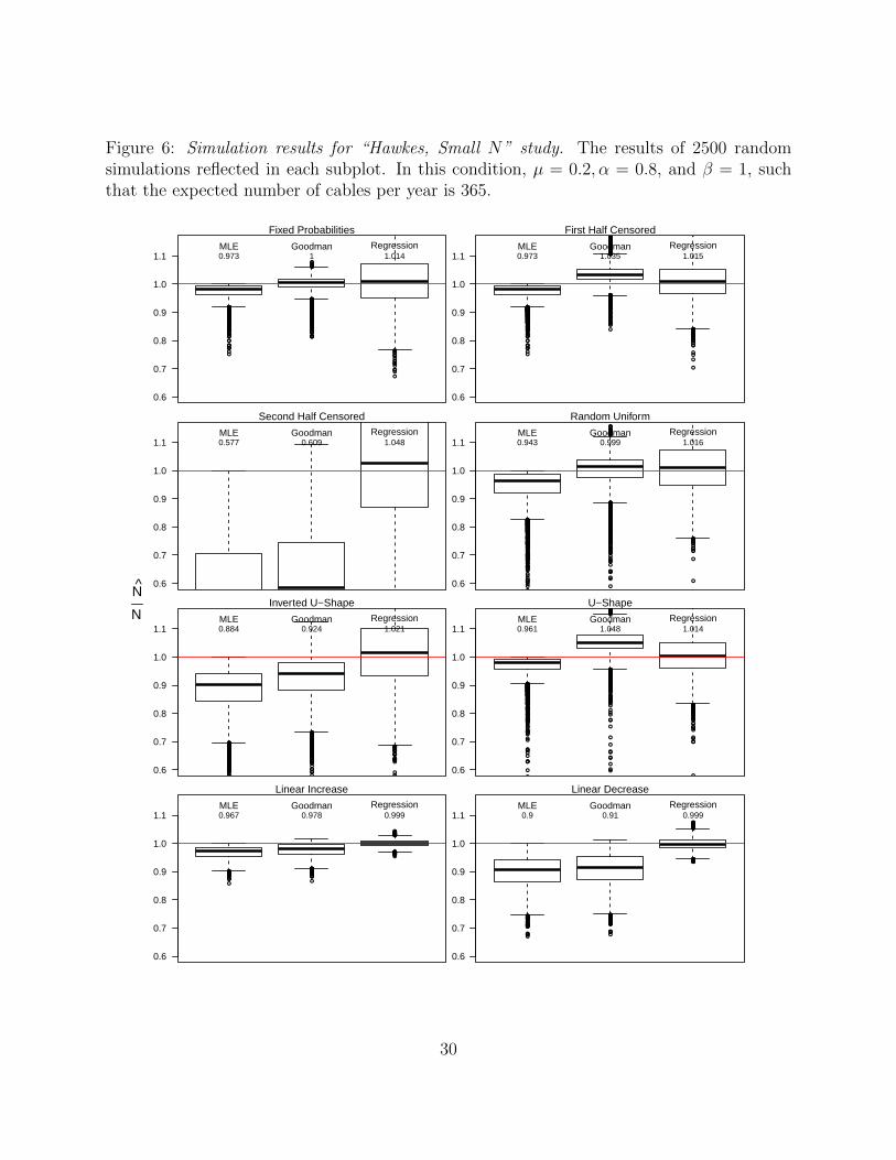
Figure 6: Simulation results for “Hawkes, Small N” study. The results of 2500 randomsimulations reflected in each subplot. In this condition, µ = 0.2, α = 0.8, and β = 1, suchthat the expected number of cables per year is 365.
●
●
●
●
●
●
●●
●
●
●
●
●●
●
●
●
●
●
●
●●●●●
●
●
●
●●●●●●●●●●●
●●●
●●●●●●
●
●
●
●●●
●●●
●
●●●
●
●
●
●●●●
●
●●●
●●●
●●
●
●
●
●●●●●●●●●●
●
●
●●
●
●●
●
●●
●
●
●
●●
●●●●●
●
●
●
●
●●
●●
●
●●
●
●●
●
●
●
●●●●●●
●
●●
●
●
●
●
●
●●●
●
●
●●
●
●
●
●●
●
●
●
●
●●●
●
●●
●●●
●●
●
●
●
●●
●
●●●●●
●
●
●
●
●●
●
●
●
●●●●●
●●
●
●
●●●
●
●
●●●●
●
●●●●
●
●
●
●
●
●
●
●
●●
●●●
●
●
●
●
●
●
●●
●
●
●
●
●
●●●
●●●
●●
●●●●
●
●
●
●●●●●●●●●
●
●
●
●
●●
●
●
●
●
●
●
●●
●●●
●
●
●●●●●●
●
●●●●
●
●
●
●
●
●
●●●●●
●
●
●
●
●●●●●●●●●●
●●●●●●●
●
●
●●
●
●●
●
●●●●
●
●
●●
●
●●
●●
●
●●
●●
●
●●
●
●●●
●●●●●●●●●
●
●
●
●
●
●
●
●
●●
●
●
●
●●
●●
●●●●●
●
●
●
●
●
●
●
●
●●
●
●●
●
●●
●
●●
●
●
●
●●
●
●
●●●
●
●
●●●
●
●
●●
●
●●
●●
●
●
●
●●●
●
●
●●
●
●
●
●●
●
●
●
●
●
●●●●●●
●
●
●
●
●
●
●
●
●
●
●
●
●●
●●
●
●
●●●
●
●●●●●●
●
●
●
●
●
●●
●
●
●●●●
●●
●●
●
●
●
●
●
●
●
●
●
●
●●
●
●●●●●●
●
●●
●●●●
●
●
●
●
●
●●
●
●●●●●
●
●
●
●
●●
●
●
●
●
●
●
●
●
●●●
●●●
●●●
●●
●
●
●
●
●
●●●●
0.6
0.7
0.8
0.9
1.0
1.1MLE Goodman Regression
Fixed Probabilities
0.973 1 1.014
●
●
●
●
●
●
●●
●
●
●
●
●●
●
●
●
●
●
●
●●●●●
●
●
●
●●●●●●●●●●●
●●●
●●●●●●
●
●
●
●●●
●●●
●
●●●
●
●
●
●●●●
●
●●●
●●●
●●
●
●
●
●●●●●●●●●●
●
●
●●
●
●●
●
●●
●
●
●
●●
●●●●●
●
●
●
●
●●
●●
●
●●
●
●●
●
●
●
●●●●●●
●
●●
●
●
●
●
●
●●●
●
●
●●
●
●
●
●●
●
●
●
●
●●●
●
●●
●●●
●●
●
●
●
●●
●
●●●●●
●
●
●
●
●●
●
●
●
●●●●●
●●
●
●
●●●
●
●
●●●●
●
●●●●
●
●
●
●
●
●
●
●
●●
●●●
●
●
●
●
●
●
●●
●
●
●
●
●
●●●
●●●
●●
●●●●
●
●
●
●●●●●●●●●
●
●
●
●
●●
●
●
●
●
●
●
●●
●●●
●
●
●●
●
●●
●
●
●
●
●
●
●●
●
●●●
●
●
●
●
●●
●●●
●●
●
●
●
●
●
●
●
●●
●●
●●●
●
●
●
●
●
●
●
●
●
●
●
●●
●
●
●
●
●
●
●
●
●
●
●●
●
●
●
●●
●
●●●
●
●
●●●
●
●
●●
●
●
●●
●●●
●
●●●
●
●
●●
●
●●
●
●
●
●●
●
●
●
●
●
●
●
●
●
●
●
●
●
●
●
●●
●
●
●●●
●
●
●●
●
●
●
●
●●●
●
●
●
●●●
●
●
●
●●
●
●●
●●●
●
●
●
●
●
●●
●
●
●●
●
●●
●●
●
●
●
●
●
●
●
●
●●
●●
●●
●
●●
●●
●
●
●●●
●●●●
●●
●
●
●
●
●
●
●
●
●
●
●
●
●
●
●
●
●
●
●
●
●●
●
●
●
●
●
●
●
●●●●
●
●
●
●●●●
●
●
●
●
●●
●
●
●●
●●
●●
●
●
●
●●
●
●
●
●
●
●
●
●
●
●
●
●
●●
●
●
●●
●
●
●●
●
●
●
●
●
●
●
●
●
●
●
●
●
●●●
●●
●
●
●
●
●
●
●●
●
●
●
●
●●
●
●
●
●
●
●
●●
●
●
●
●
●●●
●
●
●●●
●
●
●
●●
●
●
●
●
●
●
●
●
●
●
●
●
●
●
●
●
●
●
●●
●
●
●
●
●
●●
●
●
●
●
●●●
●
●
●
●●
●
●
●
●
●
●●
●
●●
●
●
●
●
●
●
●
●●
●●
●
●
●
●
●
●●
●
●
●
●
●
●
●
●
●●●
●
●
●
●
●
●
●
●
●●
●
●
●●
●
●
●
●●
●
●
●●
●
●
●●●
●●●
●●
●
●●
●●●●
0.6
0.7
0.8
0.9
1.0
1.1MLE Goodman Regression
First Half Censored
0.973 1.035 1.015
●
●
●
●
●●
●
●
●
●●
●●
●
●
●
●
●
●
●
●
●
●
●
●
●
●
●
●
●
●
●●
●●
●●
●
●
●
●
●
●
●
●
●
●
●
●
●●
●●
●●
●
●●
●
●
●●
●●●
●●●
●
●
●
●●
●●
●
●
●
●
●
●
●
●
●
0.6
0.7
0.8
0.9
1.0
1.1MLE Goodman Regression
Second Half Censored
0.577 0.609 1.048
●
●
●
●
●●
●●●
●
●
●
●
●
●
●
●
●
●●
●
●
●
●●●●
●
●
●
●
●
●
●●●●
●●●
●
●
●
●
●
●
●
●●
●
●
●
●
●
●
●●
●
●●●●
●
●
●
●●
●
●
●
●
●
●
●●
●
●
●
●
●
●
●●
●
●●●
●
●
●●
●
●
●
●
●
●
●
●
●
●
●
●
●
●●●
●
●
●
●
●
●
●
●●
●
●
●
●●●
●●
●
●
●
●
●
●
●●●●
●●●
●
●●
●
●
●●
●
●
●
●
●●
●●
●
●●
●
●
●
●
●
●●
●
●
●
●●
●
●
●
●
●
●
●
●
●
●
●
●
●
●
●
●●
●
●
●
●
●
●
●
●
●
●●
●●
●●●
●
●●●
●
●
●●
●
●●
●●
●●
●●
●●
●
●●●●
●
●
●●
●
●●
●
●
●
●
●
●
●
●
●
●●
●
●
●
●●●
●
●
●
●
●
●
●
●
●
●●
●
●
●
●
●●
●●
●
●
●●
●
●●
●
●
●
●
●
●
●
●
●●
●
●
●
●●
●
●
●
●
●
●
●
●●
●
●
●●
●●
●
●
●
●
●
●
●
●●
●
●
●●
●
●●
●
●
●
●
●
●
●●●
●
●●
●
●
●
●
●
●
●
●
●
●●●
●
●
●
●
●
●
●
●
●
●●●
●●
●
●
●●●
●
●
●
●
●●
●
●
●
●
●
●
●
●
●
●
●
●
●
●
●
●
●●●
●
●●
●
●●
●
●
●
●●
●
●
●
●
●●
●
●
●
●
●
●●
●
●
●
●
●●
●●
●●
●●●
●
●●
●
●●
●
●
●
●
●
●
●
●●●
●
●
●
●
●
●
●
●●
●
●
●●
●
●
●
●
●
●
●
●
●
●
●●●●
●
●
●
●
●
●
●
●
●●
●
●
●●
●
●
●●
●
●
●
●
●●●
●
●
●
●
●
●
●
●
●
●
●
●●
●●
●
●
●
●
●●
●
●
●
●
●●
●●
●
●●
●
●
●
●
●
●
●
●
●
●
●
●
●
●●●
●
●
●
●
●
●
●
●
●
●
●
●
●
●
●
●
●
●
●
●
●
●●●●
●
●
●
●
●
●
●
●
●
●
●●
●
●
●
●
●●
●
●
●
●
●
●
●●
●
●
●
●
●
●
●
●
●
●
●
●
●
●
●
●
●
●
●
●
●
●
●
●
●
●
●
●
●
●
●
●
●●
●
●
●
●
●
●●
●
●
●
●
●
●
●
●
●●
●
●
●
●
●
●
●
●
●
●
●
●
●
●
●
●
●
●
●
●
●
●
0.6
0.7
0.8
0.9
1.0
1.1MLE Goodman Regression
Random Uniform
0.943 0.999 1.016
●●●
●
●
●
●
●
●●
●
●●●
●
●
●●
●
●
●
●●●●●
●
●
●●
●
●
●
●
●
●
●●
●●●
●
●
●
●●●
●
●●●
●
●
●
●
●
●
●●
●
●
●●
●
●
●
●
●
●●
●
●
●
●
●
●
●●
●
●
●
●●
●
●
●
●●●●
●
●
●
●
●
●
●
●
●
●
●
●
●
●
●
●●
●
●
●
●
●●
●
●
●●
●
●
●
●
●
●
●●
●
●●
●
●●
●
●
●
●
●
●
●
●
●
●
●
●
●
●
●●●●●●●
●
●●●
●
●
●
●
●
●
●
●
●
●
●
●
●
●●
●●
●
●
●
●
●
●
●
●
●●●
●
●
●
●
●
●●
●
●
●●
●
●●
●
●
●
●
●●
●
●
●
●
●
●●
●●
●
●
●●●
●
●●
●
●
●
●
●
●
●
●
●
●●●●
●
●
●
●
●
●
●
●
●
●
●
●
●●●
●
●
●
●
●
●
●
●
●
●●●
●
●
●
●
●●
●
●
●●
●
●
●
●●
●
●
●
●
●
●
●
●
●
●●
●●●●
●
●
●
●
●●
●
●●
●
●
●
●●
●●
●
●
●●
●
●
●
●
●
●
●
●●
●●
●
●
●
●
●
●
●
●
●●
●
●
●
●
●
●
●
●
●
●
●
●
●
●
●
●
●
●
●
●●
●
●
●
●
●
●
●
●
●
●
●
●
●
●
●
●
●
●
●
●
●
●
●
0.6
0.7
0.8
0.9
1.0
1.1MLE Goodman Regression
Inverted U−Shape
0.884 0.924 1.021
●
●
●
●●
●
●
●
●
●
●
●
●
●
●
●
●●
●
●
●
●
●
●
●
●
●
●
●
●
●●
●
●
●●
●
●
●
●
●
●
●
●
●
●●
●
●
●
●
●
●
●
●
●●
●
●
●
●●
●
●
●
●
●
●
●
●●●●
●
●
●
●●●●●●
●
●
●
●●
●
●
●
●
●
●●
●
●●●
●
●
●
●
●
●●●●
●
●
●●●
●
●
●
●
●
●
●
●
●
●
●
●
●
●
●
●●●
●
●
●
●
●
●
●
●
●
●
●●
●●
●
●
●
●
●
●
●
●●●
●
●
●
●
●
●
●
●
●
●
●
●
●
●
●
●
●●●
●
●●
●
●
●
●
●
●
●
●
●
●
●
●
●
●
●●
●
●
●
●
●
●
●
●
●
●
●
●
●
●
●
●
●
●
●●●
●
●●
●
●
●
●
●
●
●
●
●
●●●
●
●
●
●
●
●
●●
●
●
●
●
●
●
●●●
●
●
●
●
●
●●
●
●
●
●
●
●●
●
●
●
●
●●
●
●●
●●
●
●●
●●
●
●
●
●
●
●
●
●
●
●
●
●
●
●●●●●
●●
●
●
●
●
●
●
●●
●
●●●
●
●
●
●
●
●
●●
●
●
●●
●
●
●
●
●
●
●●
●
●
●
●●●●●
●
●●
●
●
●
●
●
●
●
●
●
●●●●
●
●
●●●
●●
●
●
●
●
●
●
●
●
●●
●
●
●
●
●
●
●
●
●
●
●
●
●
●
●
●
●
●
●
●
●●
●
●
●
●
●
●
●
●●●
●●
●
●
●
●
●
●
●
●
●
●
●
●
●
●
●
●
●
●
●
●●
●
●
●●
●
●●
●
●
●
●
●
●
●
●
●
●
●
●●●●●
●
●
●
●
●
●
●
●
●
●
●
●●
●
●
●
●
●
●
●
●
●
●
●
●
●●●
●
●
●
●
●
●
●
●
●
●
●●
●
●
●
●
●
●
●
●
●
●
●
●
●
●●
●
●
●
●
●●
●
●
●
●
●
●
●
●
●
●●
●
●
●
●●●
●
●
●
●●
●
●
●
●●
●
●
●●●
●
●
●
●
●
●
●
●
●
●
●
●●
●
●
●
●
●
●
●
●
●
●
●
●
●
●
●
●
●
●●
●
●
●
●
●
●
●
●
●
●
●
●●
●
●
●
●●
●
●
●
●
●
●
●
●
●
●
●
●
●
●
●
●
●
●
●
●
●
●
●
●
●
●
●
●
●
●●●
●
●
●
●
●
●
●
●
●
●
●
●
●
●
●
●●
●
●
●
●
●
●
●
●
●●
●
●
●
●
●
●
●
●
●
●
●
●
●●
●
●
●●
●
●
●
●
●
●
●
●
●
●
●
●
●
●
●
●
●
●
●
●
●
●
●
●
●
●
●
●
●
●
●
●
●
●
●
●
●
●
●
●
●
●
●
●
●
●
●
●
●
●
●
●
●
●
●
●
●
●
●
●●
●
●
●
●
●
●
●
●
●
●
●
●
●
●
●
●
●
●
●
●
●●
●
●
●●
●
●
●
●
●
●
●
●
●
●
●
●
●
●
●
●
●
●
●
●
●
●
●
●
●
●
●
●
●
●●
●
●
●
●
●●
●
●
●
●
●
●
●
●
●
●
●
●
●
●
●
●
●
●
●●
●
●
●
●
●
●
●
●
●
●●
●●
●
●
●
●
●
●
●●
●
●
●
●
●
●
●●
●
●
●
●
●
●●
●
●
●
●
●
●
●
●
●
●
●
●
●
●
●
●
●
●
●●
●
●●
●
●
●
●
●
●
●
●
●
●
●
●
●
●
●
●
●
●
●
●
●●
●
●
●
●
●
●
●
●
●
●
●
●
●
●
●
●
●
●
●
●●
●
●
●
●
●
●●
●
●
●
●
●
●
●
●
●
●
●
●
●
●
●
●
●
●
●
●
●
●
●
●
●●
●
●●
●
●
●
●
●●
●
0.6
0.7
0.8
0.9
1.0
1.1MLE Goodman Regression
U−Shape
0.961 1.048 1.014
●●●●
●
●●●●●●●●●●●●
●
●●●●●●
●●●●●
●●●
●
●
●
●●●●●●●●●●
●
●●●●●●
●●
●●●
●●●●
●●
●
●●●●●●
●●
●
●●●●●●
●
●
●
●
●
●
●
●
●●●
●●
●●●
●●
●●
●●
●
●
●●●
●
●●●
0.6
0.7
0.8
0.9
1.0
1.1MLE Goodman Regression
Linear Increase
0.967 0.978 0.999
●●●
●●●●
●
●
●
●
●
●●
●
●
●●●●●
●
●●
●
●●
●
●
●●
●●●
●●●
●
●
●
●
●
●●
●
●
●●●●●●●
●
●●
●
●
●●
●
●
●
●
●
●●
●
●●●●
●
●●
●
●
●●
●●●●
●
●●●●●
●
●●●
●
●
●●
●●
●
●●●●●●
0.6
0.7
0.8
0.9
1.0
1.1MLE Goodman Regression
Linear Decrease
0.9 0.91 0.999
N
N
30

References
Christensen, Thomas. 2006. “Fostering Stability or Creating a Monster? The Rise of China
and U.S. Policy toward East Asia.” International Security 31(1).
Durbin, James. 1961. “Some methods for constructing exact tests.” Biometrika 48(1).
Fearon, James. 1994a. “Domestic Political Audiences and the Escalation of International
Disputes.” American Political Science Review 88:577–92.
Fearon, James. 1994b. “Signaling Versus the Balance of Power and Interests: An Empirical
Test of a Crisis Bargaining Model.” Journal of Conflict Resolution 38(2):236–69.
Fearon, James. 1995. “Rationalist Explanations for War.” International Organization
49(3):379–414.
Gibbs, David. 1995. “Secrecy and International Relations.” Journal of Peace Research
32(2):213–228.
Goemens, Hein. 2000. War and Punishment: The Causes of War Termination and the First
World War. Princeton, NJ: Princeton University Press.
Goodman, Leo. 1954. “Some Practical Techniques in Serial Number Analysis.” Journal of
the American Statistical Association 49(265):97–112.
Goodman, Leo A. 1952. “Serial Number Analysis.” Journal of the American Statistical
Association 47(260):622–634.
Hawkes, A.G. 1971. “Spectra of some self-exciting and mutually exciting point processes.”
Biometrika 58(1):83–90.
Hohle, Michael and Leonhard Held. 2006. Bayesian Estimation of the Size of a Population.
Technical Report Discussion Paper 499 Ludwig-Maximilians-Universitat Munchen.
31
Lake, David. 2010. “Two Cheers for Bargaining Theory: Assessing Rationalist Explanations
of the Iraq War.” International Security 35(3):7–52.
Larsen, Richard and Morris Marx. 2011. Introduction to Mathematical Statistics and Its
Applications. Upper Saddle River, NJ: Pearson.
Lewis, Peter. 1965. “Some Results on Tests for Poisson Processes.” Biometrika 52(1/2):67–
77.
Ogata, Yosihiko. 1988. “Statistical models for earthquake occurrences and residual analysis
for point processes.” Journal of the American Statistical Association 83:9–27.
Ramsay, Kristopher. 2008. “Settling It on the Field: Battlefield Events and War Termina-
tion.” Journal of Conflict Resolution 52(6):850–879.
Reed, William. 2003. “Information and Economic Interdependence.” Journal of Conflict
Resolution 47(1):54–71.
Reiter, Dan. 2009. How Wars End. Princeton: Princeton University Press.
Ruggles, Richard and Henry Brodie. 1947. “An Empirical Approach to Economic Intelligence
in World War II.” Journal of the American Statistical Association 42(237):72–91.
Sagar, Rahul. 2013. Secrets and Leaks: The Dilemma of State Secrecy. Princeton, NJ:
Princeton University Press.
Schultz, Kenneth. 1999. “Do Democratic Institutions Constrain or Inform? Contrasting Two
Institutional Perspectives on Democracy and War.” International Organization 53(2):233–
266.
Shapiro, Jacob and David Siegel. 2010. “Is this Paper Dangerous? Balancing Secrecy and
Openness in Counterterrorism.” Security Studies 19(1):66–98.
32
Slantchev, Branislav. 2006. “Politicians, the Media, and Domestic Audience Costs.” Inter-
national Studies Quarterly 50:445–477.
Smith, Alastair. 1998. “International Crises and Domestic Politics.” American Political
Science Review 92(3):623–38.
Smith, Alistair and Allan Stam. 2004. “Bargaining and the Nature of War.” Journal of
Conflict Resolution 48(6).
Snyder, Jack and Erica D. Borghard. 2011. “The Cost of Empty Threats: A Penny, Not a
Pound.” American Political Science Review 105(3).
Werner, Suzanne. 1999. “The Precarious Nature of Peace: Resolving the Issues, Enforcing
the Settlement, and Renegotiating the Terms.” American Journal of Political Science
43(3):912–934.
33
Recommended