ELASTIC FLEXURAL-TORSIONAL BUCKLING
ANALYSIS OF DOUBLY-SYMMETRICAL
WEB-TAPERED I-BEAMS
by
Shuai Zhu
B.S., Wuhan University, 2007
Submitted to the Graduate Faculty of the
Swanson School of Engineering in partial fulfillment
of the requirements for the degree of
Master of Science
University of Pittsburgh
2009
ii
UNIVERSITY OF PITTSBURGH
SWANSON SCHOOL OF ENGINEERING
This thesis was presented
by
Shuai Zhu
It was defended on
Oct. 5, 2009
and approved by
Kent A. Harries, Associate Professor, Department of Civil and Environmental Engineering
John F. Oyler, Adjunct Associate Professor, Department of Civil and Environmental Engineering
Morteza A. M. Torkamani, Associate Professor, Department of Civil and Environmental Engineering,
Thesis Advisor

iii
Copyright © by Shuai Zhu
2009
iv
ELASTIC FLEXURAL-TORSIONAL BUCKLING ANALYSIS OF
DOUBLY-SYMMETRICAL WEB-TAPERED I-BEAMS
Shuai Zhu, M.S.
University of Pittsburgh, 2009
In structural steel design, flexural-torsional buckling (FTB) is an important limit state that
must be considered, especially in thin-walled members. A thin-walled beam loaded in its
plane of symmetry bends in-plane of loading, however, it may fail because of the
flexural-torsional buckling, where the beam suddenly deflects and twists out of the loading
plane. This type of failure occurs suddenly in members with a much greater in-plane
bending stiffness than torsional or lateral bending stiffness. In this paper, the finite element
approach in conjunction with the energy method is employed to predict the flexural-torsional
buckling loads of a doubly symmetric and web-tapered I-beam.
The total potential energy of the flexural-torsional buckling of a beam element is
formulated by adding the strain energy to the potential energy of the external forces. To
apply the finite element approach, the displacement function of an element is assumed to be
cubic polynomials, the variational principle is then applied to the total potential energy
equation. Rearrangement of the energy equation leads to the elastic and geometric stiffness
matrices. To apply this methodology to the analysis of plane structures, the rotation
transportation matrix is applied to both element elastic and geometric stiffness matrices to
convert them from the local to a global coordinate system. Through the assembly process of
v
stiffness matrices of each element, with respect to the global degree of freedom, the
equilibrium equation of the whole structure is formed, which leads to a generalized
eigenvalue problem.
In out-of-plane stability problems, in-plane deflections are normally assumed to be
neglected if the ratio of the minor axis flexural and torsional stiffness to the major axis
flexural stiffness is small. The effects of prebuckling are also required when accurate
solutions are needed.
Due to the compatibility between the finite element approach and programming,
computer technology is utilized in the analysis to extend the application of the method
developed in this paper to much more complex structures, which involves enormous
computations. Object-oriented technology in C++ is employed to help organize the
programming process. Several examples are presented to compare the results to show the
efficiency of developed principles.
vi
TABLE OF CONTENTS
1.0 INTRODUCTION…………………………………………..…………..……….…….................................1
2.0 LITERATURE REVIEW…………………………………………………….....................................…3
2.1 FLEXURAL-TORSIONAL BUCKLING…..………….......................................3
2.2 FLEXURAL-TORSIONAL BUCKLING OF TAPERED STRUCTURES....5
3.0 FLEXURAL-TORSIONAL BUCKLING THEORY………………………….......................8
3.1 DERIVATION OF ENERGY EQUATIONS.................................................12
3.1.1 Strain Energy..............................................................................13
3.1.2 Displacements............................................................................15
3.1.3 Strains........................................................................................24
3.1.4 Stress and Stress Resultants.......................................................25
3.1.5 Section Properties......................................................................26
3.1.6 Strain Energy Equation..............................................................27
3.2 POTENTIAL ENERGY OF THE LOADS..................................................27
3.2.1 Displacements...........................................................................29
3.2.2 Potential Energy of Loads Equation.........................................30
vii
3.3 ENERGY EQUATION......................................................................................30
4.0 DERIVATION OF SECTION PROPERTIES OF A DOUBLY-SYMMETRIC WEB-TAPERED I-BEAM…………………………………………..…..………………..…….……………..….……32
4.1 APPLICATION OF ROTATION TRANSFORMATION EQUATION IN A DOUBLY-SYMMETRIC WEB-TAPERED CROSS SECTION.................................33
4.1.1 Rotation Transformation Equation in the Web.................................35
4.1.2 Rotation Transformation Equation in the Flange.............................36
4.2 FINITE NORMAL STRAIN...........................................................................38
4.3 DERIVATION OF SECTION PROPERTIES.................................................39
4.3.1 Axial Deformation...........................................................................39
4.3.2 Bending about x-axis.......................................................................42
4.3.3 Bending about y-axis.......................................................................45
4.3.4 Free Torsional Deformation.............................................................48
4.3.5 Warping Strain of the Flanges Due to Free Torsional Deformation……………………………………………………………………………..….………………50
4.4 CONCLUSTION.............................................................................................53
5.0 FINITE ELEMENT METHOD……………………….……………………………………..…………….54
5.1 DERIVATION OF TRANSFORMATION MATRIX T AND eT ……….……..60
5.1.1 Derivation of Transformation Matrix T ………………………………..…….61
5.1.2 Derivation of Transformation Matrix eT ………………………….…….……64
5.2 DERIVATION OF ELASTIC STIFFNESS MATRIX eK ……………..……………68
viii
5.2.1 Elastic Stiffness Matrix of the Web…………….……….……..…………….…..…68
5.2.2 Elastic Stiffness Matrix of the Flange……………………………...….…………..70
5.3 DERIVATION OF GEOMETRIC STIFFNESS MATRIX eG ………………….…..72
6.0 FLEXURAL-TORSIONAL BUCKLING EIGENVALUE PROBLEM
SOLUTION……………………..………………..……………….................……………………..…….……....…......75
7.0 SOFTWARE DEVELOPMENT………………..………………....……………………….….………..…79
7.1 OBJECT-ORIENTED MODELING AND PROGRAMMING
CONCEPTS……………………………………………………………………………….………………………..……80
7.2 PROGRAM DESIGN…..……….……………….……………………………………..……...……..85
7.3 OBJECT-ORIENTED MODELING AND PROGRAMMING FLEXURAL
TORSIONAL BUCKLING PROBLEMS …..……….…………………..…..……….…………...…..88
7.3.1 Inception…..…………….…..……………..…………………….………...………..…….88
7.3.2 Elaboration…..……………..…………….…..………………..……….…………...……88
7.3.3 Construction…..……………..……..…………..…………………………..….…………90
7.3.4 Transition…..……..……………..………………..…………………….…….…………109
8.0 CASES OF FLEXURAL-TORSIONAL BUCKLING………………...................…….110
8.1 BUCKLING ANALYSIS: EXAMPLE 1……………………..……….…………...….….110
8.2 BUCKLING ANALYSIS: EXAMPLE 2……………………..……………..………….…114
8.3 BUCKLING ANALYSIS: EXAMPLE 3……………………..….……………..….…....121
8.4 CONCLUSION……………………..……………………………..………….……………...…......126
ix
9.0 SUMMARY………………………………..…………………………………………..………………….…….……128
APPENDIX A………………………………………………………...………..……….….………..……….………..132
DERIVATION OF THE ROTATION TRANSFORMATION MATRIX….…..….……….132
A.1 VECTOR oR ………………………………………….………..…………….…………………….…...133
A.2 VECTOR RL ………………………………………….………..………………………………….…….134
A.3 VECTOR LQ ………………………………………….………..………………………….……..…….135
A.4 FINITE DISPLACEMENTS TRANSFORMATION …………………………….…….137
A.5 ROTATION TRANSFORMATION MATRIX ……………..……….......................139
APPENDIX B……………………………..…...………………………………………………………………..…………..144
B.1 ELASTIC STIFFNESS MATRIX OF A WEB ELEMENT…………………….….144
B.2 ELASTIC STIFFNESS MATRIX OF A FLANGE ELEMENT………………...148
B.3 GEOMETRIC STIFFNESS MATRIX OF A BEAM ELEMENT……………...151
APPENDIX C.………………..……………………………………………….……………………......................…154
FLEXURAL-TORSIONAL BUCKLING ANALYSIS PROGRAM……………….......154
C.1 PROP.H ……………..………………..………………..………………..………………………....……154
C.2 ELEMENTSTIFF.H ……………..………………………………………………..…..……………155
C.3 ELEMENTGEOM.H ……………..………………………………………………...……………..156
C.4 STIFFN.H ……………..……………………………………………………………..................….157
C.5 GEOMTR.H ……………..……………………………………………………..………….…………..157
x
C.6 SPPRT.H …………..…………………………..…………………………….……………………………….158
C.7 STANDM.H ……………..…………………………………………………………….………….…….….158
C.8 PROP. CPP ………………………………………………………………………………..………………...159
C.9 ELEMENTSTIFF. CPP ……………..……………………………………………….………………..160
C.10 ELEMENTGEOM. CPP ……………..…………………….………………………………………...168
C.11 STIFFN. CPP ……………..…………………………………………………………….………………....171
C.12 GEOMTR. CPP …………….…………………………………………………...………………………..172
C.13 SPPRT. CPP ……………..……………………………………………..………………….…………..…..173
C.14 STANDM. CPP ……………..…………………………………………………….…………………..….175
C.15 LBUCK. CPP ……………..…………………………………………………………….………………...182
BIBLIOGRAPHY…………………………….……....……………………………..………..……….…….………….185

xi
LIST OF TABLES
A- 1 Direction Cosines ..........................................................................................................142
xii
LIST OF FIGURES
3.1 Coordinate System................................................................................................................9
3.2 Cross Section View Displacements.....................................................................................10
3.3(a) Top View Displacement..................................................................................................10
3.3(b) Bottom View Displacement............................................................................................10
3.4 External Loads and Member End Actions of the Beam Element .......................................11
3.5 Deformed Element..............................................................................................................16
3.6 Undeformed Element z∆ and Deformed Element (1 )z ε∆ + ........................................19
3.7 Twist Rotation ...................................................................................................................20
4.1 Coordinate Systems............................................................................................................32
4.2 Cross Section Diameters....................................…………………….…………………………….…….….34
4.3(a) Cross Section View with an Arbitrary Point P ............................................................35
4.3(b) Displacements of the Point P .....................................................................................35
4.4(a) Cross Section View with an Arbitrary Point Q .........................................................37
4.4(b) Displacements of Point Q ..........................................................................................37
xiii
5.1 The Element Degrees of Freedom………………………………….………………………………………….…..57
5.2 The Depth of the I-Beam……………………………………...……..……………………………………….……….58
5.3 Displacements of the Centroid of the Web and the Flanges……………….…………………………..60
5.4 Transformation of the Displacement at the Centroid of the Flanges……............................61
5.5 Relation Between Displacements of the Web and the Flanges…………………………………..…...64
7.1 The Object-oriented Paradigm............................................................................................81
7.2 Class Illustration................................................................................................................83
7.3 Inheritance Illustration......................................................................................................84
7.4 Rational Unified Process...................................................................................................87
7.5 Refactoring Process...........................................................................................................90
7.6 Possible LBuck Program Classes......................................................................................91
7.7 Modeling Procedure..........................................................................................................92
7.8 Example Class Diagram.....................................................................................................93
7.9 LBuck Program Classes.....................................................................................................94
7.10 LBuck Program Class Diagram........................................................................................95
7.11 LBuck Program Sequence Diagram.................................................................................98
7.12 Activity Diagram............................................................................................................101
8.1 Lateral Buckling of Uniform I-beam…………………………………………………………………..……....111
8.2 Buckling Load: Cantilever Beam with Concentrated Load (L=10 m) ..............................................................................................................112
xiv
8.3 Non-Dimensional Analysis: Cantilever with Concentrated Load....................................113
8.4 Comparison of Buckling Loads........................................................................................127
8.5 Lateral buckling of a cantilevered doubly-symmetric I-beam under
end moments……………………………….…………………………………….…………….….…..………..115
8.6 Non-Dimensional Analysis: A Cantilevered I-Beam with End Moments…………………………………………………………………………………………………....……116
8.7 Lateral buckling of simply supported I-beams………………………………………………….…...……117
8.8 Non-Dimensional Analysis: A Simply-supported I-Beam in
Uniform Bending…………………………..…………………………………..……….……………..……117
8.9 Side-view of An Overhanging Beam………………………………...…………………………….………….119
8.10 Lateral Buckling of An Overhanging Segment in Uniform Bending............................119
8.11 Non-Dimensional Analysis: An Overhanging Segment in
Uniform Bending……………………………..…………………………………..…...…………..…………….….120
8.12 Non-Dimensional Analysis: Buckling Under End Moments.........................................121
8.13 Lateral Buckling of Web-tapered Simply Supported Beams.........................................122
8.14 Buckling Load: Simply-Supported Beam with Equal End Moments………………..….…...123
8.15 Taper Effects: Simply-Supported Beam With Two Equal End
Moments………………………………….……..………………………………………….……………..……...…....124
8.16 Comparison of Buckling Loads....................................................................................125
8.17 Comparison of Errors Under Different Taper Ratios....................................................126
A. 1 Rigid Body Movement………………………………………………………..…………………………..……….132
A. 2 Rigid Body Rotation…………………………………………………………………………………………….…..141
xv
NOMENCLATURE
Symbol Description
A Area of member
a distributed load height
[C] Cholesky matrix
D global nodal displacement vector for the
structure
D e global nodal displacement vector for an
element
d e local nodal displacement vector for an
element
E modulus of elasticity
e concentrated load height
F axial load
Fi axial loads at node i
Fj axial loads at node j
G shear modulus
h depth of the member
hi depth of the member at node i
hj depth of the member at node j
[I ] identity matrix
Ix moment of inertia about the x- axis
xvi
In moment of inertia about the n- axis
Iy moment of inertia about the y- axis
Iω warping moment of inertia
J torsional constant
kz torsional curvature of the deformed element
[Ke ]web web global elastic stiffness matrix
[Ke ]flange flange global elastic stiffness matrix
[Ke ] structure global elastic stiffness matrix
[Kg] structure global geometric stiffness matrix
L member length
Lf member length of the flange
Mx bending moment about x- axis
Mi moment at node i of the web
Mif moment at node i of the flange
Mj moment at node j of the web
Mjf moment at node j of the flange
[N] shape function matrix
P concentrated load
q distributed load
[T e] transformation matrix
tp perpendicular distance to P from the
mid-thickness surface
U strain energy
Ue strain energy for each finite element
u out-of-plane lateral displacement
up out-of-plane lateral displacement
xvii
of point P
uq out-of-plane lateral displacement
of point Q
ui ,uj out-of-plane lateral displacements at nodes i and j
u′ out-of-plane rotation
Vi shear at node i of the web
Vif shear at node i of the flange
Vj shear at node j of the web
Vjf shear at node j of the flange
v in-plane bending displacement
vP displacement through which the concentrated
load acts
vq displacement through which the distributed load
acts
v′ in-plane rotation
w axial displacement
wF longitudinal displacement through which the axial
load acts
wp longitudinal displacement of point Po
zP concentrated load location from
left support
α0 tapered angle
εp longitudinal strain of point Po
φ out-of-plane twisting rotation
φ ′ out-of-plane torsional curvature
γp shear strain of point Po
λ buckling parameter
Π total potential energy

xviii
σp longitudinal stress of point Po
τp shear stress of point Po
ω warping function
Ω potential energy of the loads
θ rotation of the member cross section
1
1.0 INTRODUCTION
Thin-walled structural elements having cross sections such as I, T, L, and C, with isotropic or
anisotropic composite materials are extensively used as beams, columns, and beam-columns
in engineering applications, ranging from buildings, bridges to aerospace and many other
engineering fields where requirements of a high performance in terms of minimum weight for
a given strength are of importance. Due to their particular shapes resulting from the
fabrication process, these elements always have open cross sections that make their behavior
highly sensitive to torsion, instabilities and imperfections (Mohri et al. 2003 and 2008). The
buckling behavior of thin-walled structures and structural elements is very complex due to
the coupling effect of compression, bending, and torsional deformations.
Presently, web-tapered thin-walled I-beams are used extensively in engineering
construction due to their structural and economic efficiency. The stability issue concerning
this type of structure has been receiving increased attention from engineers and researchers.
To take full advantage of the benefits of tapered beams, a design engineer has to be equipped
with reliable and efficient methods of analysis to give accurate predictions of the tapered
structure behavior. Lee et al. (1975) studied the behavior of tapered members extensively,
and their work was adopted in Appendix F3 of the AISC specification (Manual 1994). At
present, the general design approach used in the AISC Specification (Manual 2009) for the
2
design of web-tapered beams is to apply modification factors to convert the tapered members
into appropriately proportioned prismatic members in order that the prismatic LRFD beam
equations may be applied. This procedure is mostly applicable to a simple analysis of
tapered members. Therefore, there is a need to investigate and understand the behavior of
tapered beams to develop a method that aids engineers to use numerical methods to analyze
more complex tapered structures.
With recent advances and new development in computing technologies, complex
problems that were almost impossible to solve by the classical methods now can effectively
be solved using the numerical approach. Among many numerical methods, the finite
element method is one of the most powerful in handling complicated loadings, boundary
conditions and geometry. Furthermore, the finite element method is compatible with the
software development, because it implements in the matrix form that is suitable to use in the
discretized calculation.
The intent of this paper is to illustrate the practical application of the finite element
method in the flexural-torsional buckling analysis of doubly symmetric web-tapered I-beams.
A tapered I-beam is synthesized from two rectangular flat plates for flanges and a tapered flat
plate for the web, these plates form a rigid cross-section for the beam. The total potential
energy equation of the tapered I-beam is directly formulated from summing all the
sub-potential energy equations of these narrow beams.
3
2.0 LITERATURE REVIEW
2.1 FLEXURAL-TORSIONAL BUCKLING
The first theoretical research into elastic flexural-torsional buckling problem was preceded by
Euler’s 1759 treatise on column flexural buckling, which gave the first analytical method to
predict the reduced strengths of slender columns, and by Saint Venant’s 1855 memoir on
uniform torsion, which gave the first reliable description of twisting response of members to
torsion (Trahair 1993). However, it was not until 1899 that the first published discussions
of flexural-torsional buckling were made by Prandtl (1899) and Michell (1899), who
considered the lateral buckling of beams with narrow rectangular cross-sections.
Subsequent work by Wagner (1929) and later work by Bleich (1952) and also by
Timoshenko and Gere (1961) led the development of a general theory of flexural-torsional
buckling. They provided the classical energy equation for calculating the elastic
flexural-torisonal buckling loads of thin-walled beams.
Galambos (1963) introduced inelastic behavior of the flexural-torsional buckling;
similar research was also presented by Lee (1960), White (1956), Wittrick (1952), and Horne
(1950). All of these researches were done using the classical method, which provided exact
solutions, yet it is limited by the necessity to make extensive calculations by hand.
4
This situation changed dramatically with the advent of digital computers in the 1960’s.
Researchers used numerical approaches that worked well with computers. There were many
publications on various numerical approaches, such as Rayleigh Ritz method by Wang (1994),
the finite difference method by Bleich (1952), Assadi and Roeder (1985), and Chajes (1993),
and the finite integral method by Trahair (1968), Anderson and Trahair (1972), and
Kitipornchai and Trahair (1975).
The finite element method was introduced by Barsoum and Gallagher (1970), in which
they derived the stiffness equations for flexural-torsional instabilities of one-dimensional
members with constant cross sections. During the later research, Powell and Klingner (1970)
presented a lateral buckling analysis of an I-section beam, Hancock and Trahair (1978)
considered the lateral buckling analysis of a monosymmetric cross-section beam with
continuous restraints, Sallstrom (1996), Bradford and Ronagh (1997), and Papangelis et al.
(1998) calculated the flexural-torsional buckling loads of beams, beam-columns, and plane
frames, and Bazeos and Xykis (2002) presented research using the finite element method to
analyze three dimensional trusses and frames.
More recent research on the theory of flexural-torsional buckling has been presented
by Tong and Zhang (2003a) and (2003b) with their investigations of a new theory to clarify
the inconsistencies of existing theories of the flexural-torsional buckling of thin-walled
members. Torkamani and Roberts (2009) studied the elastic flexural-torsional buckling
analysis of plane structures by considering second variation of the total potential energy of
beam-column element and finite element method.
5
Many of the developments of the flexural-torsional buckling theory have been made
by extensions of the previously accepted theories, as expressed either by the differential
equations of elastic bending and torsion or by energy equation for buckling. The classical
energy equations for calculating the elastic flexural-torsional buckling load of thin-walled
beams are usually assumed to be independent of the prebuckling deflections.
2.2 FLEXURAL-TORSIONAL BUCKLING OF TAPERED STRUCTURES
The static analysis of thin-walled beams with variable cross-section can be dated back to the
early works in 1960s by Cywinski (1964), Bazant (1965), Lee (1967) and Wilde (1968).
During that period, researchers carried out extensive analytical works for the torsional
response of tapered beams.
Later on, the first study on the flexural-torsional buckling of doubly and singly
symmetric tapered I beams was conducted by Kitipornchai and Trahair (1972, 1975), who
described the tapering effect of web-depth on the lateral buckling of tapered I-beams due to
the transverse loads that their positions of application are above and below the shear centers.
In recent years, with the rapid growth of high-performance computers, the finite element
method has primarily become an efficient tool for dealing with the numerical analysis of
complex structural problems. Yang and Yau (1987), Bradford and Cuk (1988) developed a
general finite element model to investigate the instability of a doubly symmetric tapered
I-beam subjected to various loads. Taking account of the rotational nature of applied end
6
torques, Yau et al. (1992) derived some closed form solutions for the buckling of torsionally
loaded bars with various variable circular cross-sections by an analytical method. Starting
from Yang and Kuo’s elasticity approach (1994), Yang et al. (1996) presented an incremental
equation of equilibrium for a straight tapered solid beam, in which the effects of instability
caused by the initial forces acting on the beam element in deformed position have all been
taken into consideration. One feature of Yang et al.’s buckling theory (1994, 1996) is that
no assumption concerning the retaining and omission of higher-order terms was made in the
expression of potential energy. Based on the membrane theory of shell and Valsov’s (1961)
assumption of negligible shear strain in the middle surface of thin-walled section, Wekezer
(1985) and Rajasekaran (1994) derived the nonlinear equations for the buckling and dynamic
stability analyses of tapered beams with general thin-walled open cross-section. However,
such formulations were shown to be inconsistent, because either the shear center locations
were not adequately handled or the derivation of the nonlinear strain and displacement
relations omitted relevant terms (Andrade et al. 2005).
Pasquino and Marotti-de-Sciarra (1992) and Ronagh et al. (2000) adopted variational
principle to develop a finite element model of thin-walled members with variable open
cross-section for lateral stability analysis and obtained expressions for the first and second
variations of the beam total potential energy. This theory was solely specified and
numerically implemented for doubly symmetric cross-sections and then applied to study the
flexural-torsional buckling of webs and flange-tapered simply supported I-beams and
cantilevers acted by point loads (Andrade et al. 2005). Andrade and Camotim (2007) extend

7
this application of the general variational formulation to the study of the lateral-torsional
buckling of singly symmetric thin-walled tapered beams using the finite element method.
They presented derivation, and validate and illustrate the application. And recently, Zhang
and Tong (2008) analyzed the lateral buckling of web-tapered I-beams and developed the
total potential energy equations based on the classical variational principle for buckling
analysis.
In this work, a tapered I-beam is synthesized from three flat plates: the top flange, the
web, and the bottom flange. As a result, the total potential energy equation of a tapered
I-beam can be formulated by summing up all the sub-potential energy equations of the three
flat plates. The elastic and geometric stiffness matrices of a tapered I-beam element may be
obtained from the total potential energy equation derived using finite element method.
8
3.0 FLEXURAL-TORSIONAL BUCKLING THEORY
Beams, which are loaded in their minor principal plane and have smaller lateral and torsional
stiffness compared to their in-plane of loading stiffness or that have inadequate lateral
restraints, may buckle out of plane of the transverse load. For a perfectly straight, elastic
beam, there are no out-of-plane deformations until the load reaches a critical value, at which
point the beam buckles by deflecting laterally and twisting. The lateral deflection and
twisting are interdependent. When the beam deflects laterally, the induced moment exerts a
component torque about the deflected longitudinal axis which causes the beam to twist.
Such buckling behavior has been referred to as flexural-torsional buckling.
Flexural-torsional buckling may significantly decrease the load capacity of a member;
therefore, it is important to obtain the flexural-torsional buckling loads of a member to
provide an upper limit on the member’s strength.
To solve the problem effectively, a mathematical model is created based on the
following assumptions.
1. The entire structure remains elastic prior buckling. In order to achieve this, we
assume that the members are long and slender. It is assumed that x yI I> for
entire length of the beam.
9
2. The cross-sections of the members of the structure are doubly symmetric.
3. The member of the structure is perfectly straight and free of imperfection. The
plane of the cross section does not distort after buckling.
4. The axial displacement and the bending displacements are small and are thus
neglected.
5. The material properties do not change.
6. Local buckling of any member of the structure is not considered.
α0
x
y
zo
1
2
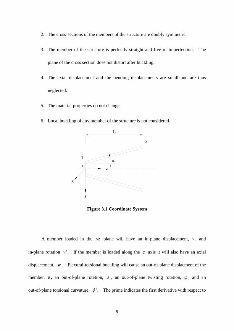
Figure 3.1 Coordinate System
A member loaded in the yz plane will have an in-plane displacement, v , and
in-plane rotation 'v . If the member is loaded along the z axis it will also have an axial
displacement, w . Flexural-torsional buckling will cause an out-of-plane displacment of the
member, u , an out-of-plane rotation, 'u , an out-of-plane twisting rotation, ϕ , and an
out-of-plane torsional curvature, 'φ . The prime indicates the first derivative with respect to
10
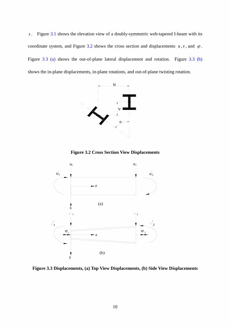
z . Figure 3.1 shows the elevation view of a doubly-symmetric web-tapered I-beam with its
coordinate system, and Figure 3.2 shows the cross section and displacements u , v , and ϕ .
Figure 3.3 (a) shows the out-of-plane lateral displacement and rotation. Figure 3.3 (b)
shows the in-plane displacements, in-plane rotations, and out-of-plane twisting rotation.
u
v
ϕ
Figure 3.2 Cross Section View Displacements
u1 u2
u'1 u'
2
'1
'2
ϕ ϕ
(a)
(b)
z
x
z
y
21
1 2
Figure 3.3 Displacements, (a) Top View Displacements, (b) Side View Displacements
11
It is assumed that the axial displacement, w , the in-plane bending displacement, v ,
and in-plane bending rotation, 'v , are small and neglected in buckling load calculations.
Only the out-of-plane displacements, u , out-of-plane rotations, 'u , out-of-plane twisting
rotation, ϕ , and out-of-plane torsional curvature, 'ϕ , will be considered to derive the
energy equation.
M1
F
P
q
F
V1V2
e a
Zp
z
y
L
M2
z z
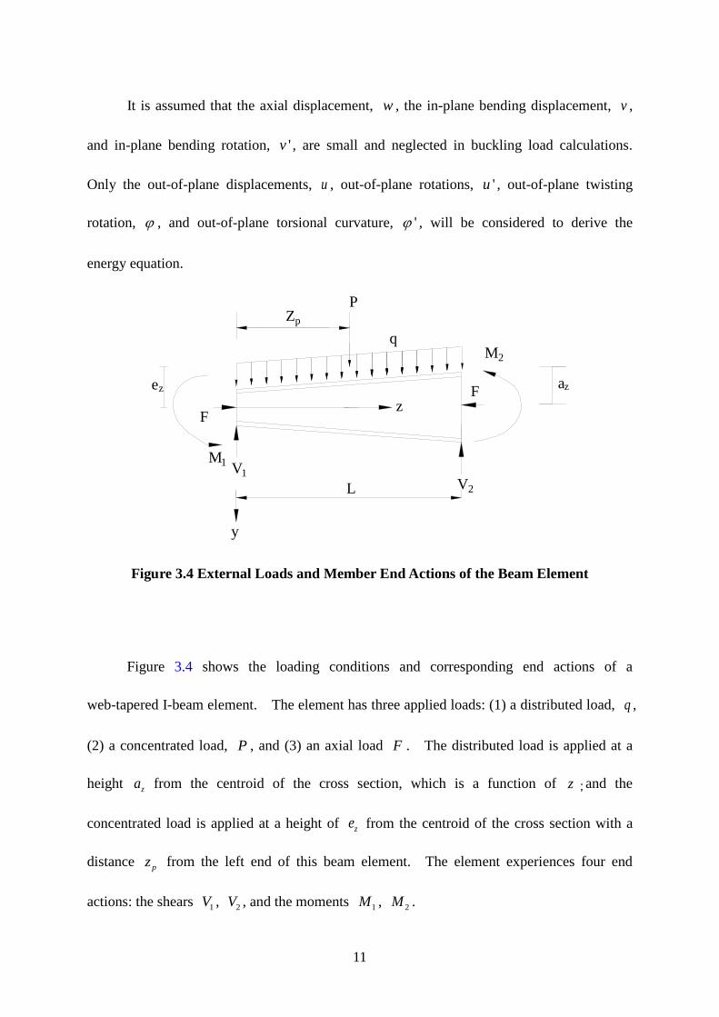
Figure 3.4 External Loads and Member End Actions of the Beam Element
Figure 3.4 shows the loading conditions and corresponding end actions of a
web-tapered I-beam element. The element has three applied loads: (1) a distributed load, q ,
(2) a concentrated load, P , and (3) an axial load F . The distributed load is applied at a
height za from the centroid of the cross section, which is a function of z ;and the
concentrated load is applied at a height of ze from the centroid of the cross section with a
distance pz from the left end of this beam element. The element experiences four end
actions: the shears 1V , 2V , and the moments 1M , 2M .
12
3.1 DERIVATION OF ENERGY EQUATIONS
The total potential energy, ∏ , of a structure is the sum of the strain energy, U, and the
potential energy of the external loads, Ω , which leads to the energy equation given by
∏ = U +Ω (3-1)
The theorem of stationary total potential energy states that of all kinematically
admissible deformations, the actual deformations (those which correspond to stresses which
satisfy equilibrium) are the ones for which the total potential energy assumes a stationary
value, i.e., the extreme value (Pilkey et al. 1994)
0δ ∏ = (3-2)
The second variation of the total potential energy equals to zero indicates the transition
from a stable state to an unstable state (Pi et al. 1992(a)), which is the critical condition for
buckling and can be expressed as
21 0
2δ ∏ = (3-3a)
therefore, the equilibrium position is stable when
21 0
2δ ∏ ≥ (3-3b)
And the equilibrium position is unstable when
21 0
2δ ∏ ≤ (3-3c)
13
Substituting in for the strain energy and the potential energy of the external loads from Eq.
(3-3a) gives
2 21 ( ) 0
2Uδ δ+ Ω = (3-4)
3.1.1 Strain Energy
An arbitrary point 0P on a cross section of the member is considered, and the strain energy,
U , in total potential energy equation of Eq. (3-1) can be expressed as
1 ( )2 P P P P
LA
U dAdzε σ γ τ= +∫∫ (3-5)
Where
Pε = longitudinal strain of point 0P
Pσ = longitudinal stress of point 0P
Pγ = shear strain of point 0P
Pτ = shear stress of point 0P
The second variation of Eq. (3-5) is
2 2 21 1 ( )2 2 P P P P P P P P
LA
U dAdzδ δε δσ δγ δτ δ ε σ δ γ τ= + + +∫∫ (3-6)
14
The strains of point 0P are defined in terms of the deformations of this point. The
longitudinal finite normal strain may be expressed as (Boresi et al. 1993)
2 2 21 [( ) ( ) ( ) ]
2p p p p
P
dw du dv dwdz dz dz dz
ε = + + + (3-7)
Where
Pu = the out-of-plane of loading lateral displacement at point 0P on the cross section.
Pv = the in-plane of loading bending displacement at point 0P on the cross section
Pw = the longitudinal displacement at point 0P on the cross section
The longitudinal displacement Pw is assumed to be small compared to the other
displacements, that is, 2( )pdwdz
is small compared to 2( )pdudz
and 2( )pdvdz
. Therefore, Eq.
(3-7) can be simplified to
2 21 [( ) ( ) ]
2p p p
P
dw du dvdz dz dz
ε = + + (3-8)
The shear strain due to bending and warping of the thin-walled section may be
disregarded. The shear strain at point 0P of the cross section due to St. Venant torsion can
be defined as (Vlasov 1961)
2P st P
dtdzφγ γ= = − (3-9)
15
The term Pt is the perpendicular distance of point 0P from the mid-thickness line of
the cross-section. The first and the second variation of the shear strain are
2P P
dtdzδφδγ = − (3-10)
2 0Pδ γ = (3-11)
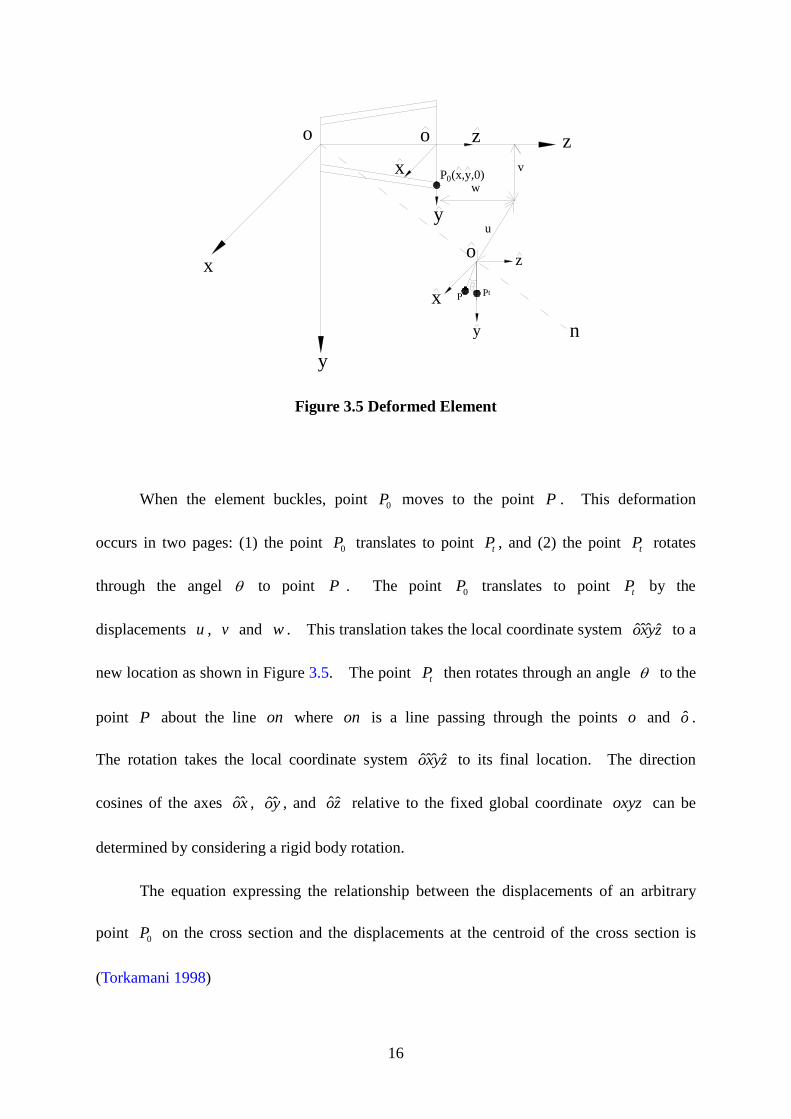
3.1.2 Displacements
The displacements Pu , Pv , and Pw of point 0P on the cross section need to be defined in
terms of the centroidal deformations u , v , and w . The deformation of an element is
shown in Figure 3.5. The coordinates oxyz represents a fixed global coordinate system
where point o is located at the beginning of the undeformed element. The ox and oy
axes coincide with the principal axes of the undeformed element. The oz axis is oriented
along the length of the element and passes through the element’s centroid. The point 0P is
defined as an arbitrary point on the cross section of the element. The coordinate ˆˆˆ ˆoxyz
represents a moving, right-handed, local coordinate system which is fixed at a point o on
the centroidal axis of the beam and moves with the beam as it deforms. The axis ˆˆoz
corresponds to the tangent at o to the deformed centroidal axis. The ˆˆox and ˆˆoy axes
are the principal axes of the deformed element. The coordinates of point 0P are ( x , y , 0)
with respect to the local coordinate system.
16
x
y
zo z
P0
PtP
n
y
z
y
(x,y,0)
u
w
v
ox
x
o
Figure 3.5 Deformed Element
When the element buckles, point 0P moves to the point P . This deformation
occurs in two pages: (1) the point 0P translates to point tP , and (2) the point tP rotates
through the angel θ to point P . The point 0P translates to point tP by the
displacements u , v and w . This translation takes the local coordinate system ˆˆˆ ˆoxyz to a
new location as shown in Figure 3.5. The point tP then rotates through an angle θ to the
point P about the line on where on is a line passing through the points o and o .
The rotation takes the local coordinate system ˆˆˆ ˆoxyz to its final location. The direction
cosines of the axes ˆˆox , ˆˆoy , and ˆˆoz relative to the fixed global coordinate oxyz can be
determined by considering a rigid body rotation.
The equation expressing the relationship between the displacements of an arbitrary
point 0P on the cross section and the displacements at the centroid of the cross section is
(Torkamani 1998)
17
ˆˆˆˆ[ ]
0
p
p R
p z
u u x xv v T y yw w kω
= + − −
(3-12)
Where
u = the out-of-plane of loading displacement at the centroid of the cross section.
v = in-plane of loading displacement at the centroid of the cross section
w = longitudinal displacement at the centroid of the cross section
x = x -coordinate of the point 0P
y = y -coordinate of the point 0P
zk = torsional curvature of the deformed element
ω = warping function (Pi et al. 1992(b))
[ ]RT = rotation transformation matrix
The first term on the right side in Eq. (3-12) stands for the translation from the point
0P to tP . The combination of the second and the third term represents the rotation part of
the total displacement due to the rotation θ . zkω− is the warping displacement defined as
the deformation in z direction. [ ]RT is the rotation transformation matrix giving the
direction cosines of the rotated axes ˆˆox , ˆˆoy , and ˆˆoz relative to the fixed axes ox , oy ,
and oz by considering a rigid body rotation of the axes through an angle θ about the axis
on .
18
From Appendix A, the rotation transformation matrix [ ]RT can be expressed for small
angles of rotation as
[ ]
2 2
2 2
22
122 2 2
12 2 2 2
12 2 2 2
x yy x zzz y
x y y zx zR z x
x z y z yxy x
T
θ θθ θ θθ θ θ
θ θ θ θθ θθ θ
θ θ θ θ θθθ θ
− +− − +
= + − − − + − + + − −
(3-13)
where xθ , yθ , and zθ are the components of the rotation θ in the x -, y -, and z - axes,
respectively.
cosxθ θ α= (3-14)
cosyθ θ β= (3-15)
coszθ θ γ= (3-16)
where α , β , and γ are the angles between the rotational axis and x -, y -, and z - axes,
respectively; θ is the rotation of the cross-section about the rotational axis.
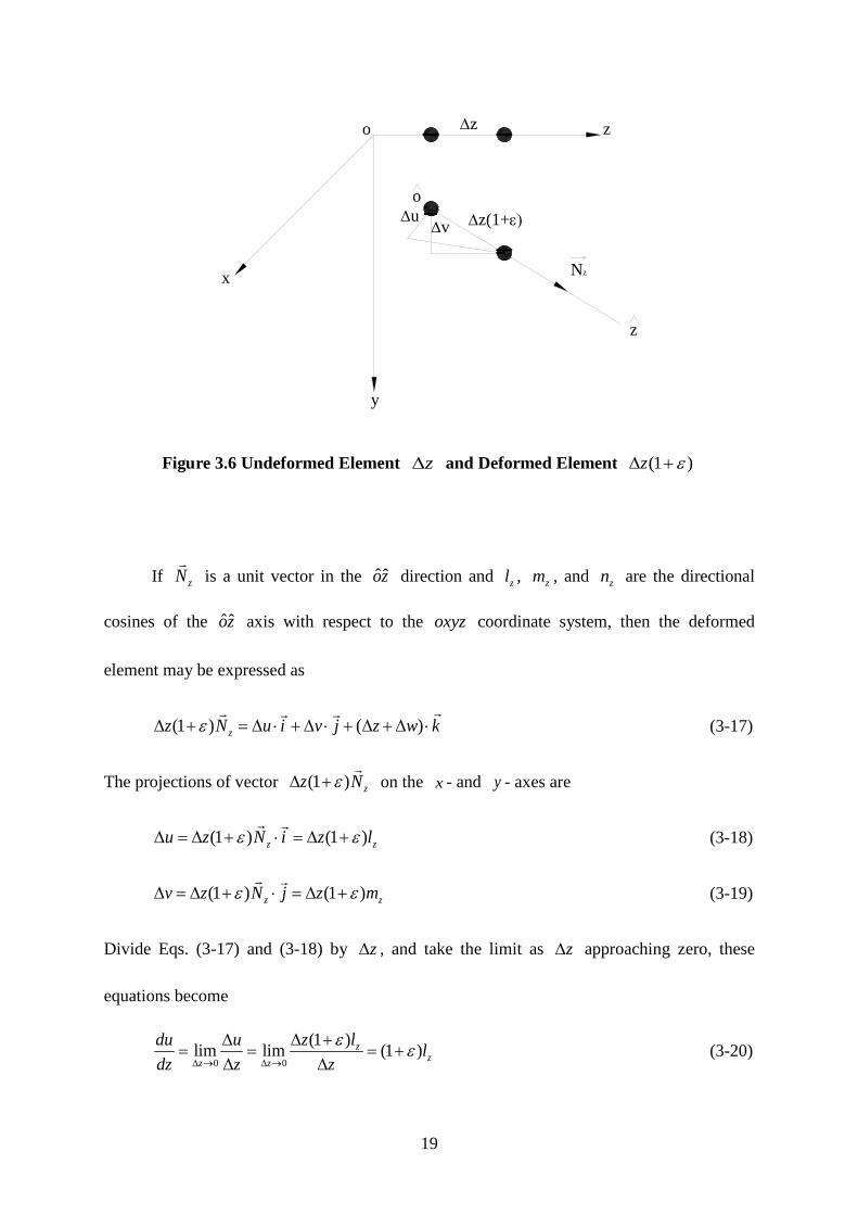
Considering the undeformed element z∆ and the deformed element (1 )z ε∆ + ,
where ε is the strain. The deformed element (1 )z ε∆ + has components u∆ , v∆ , and
( )z w∆ + ∆ on the ox , oy , and oz axes, respectively, as shown in Figure 3.6.
19
o ∆z z
x
∆u ∆z(1+ε)
Nz
y
∆v
z
o
Figure 3.6 Undeformed Element z∆ and Deformed Element (1 )z ε∆ +
If zN
is a unit vector in the ˆˆoz direction and zl , zm , and zn are the directional
cosines of the ˆˆoz axis with respect to the oxyz coordinate system, then the deformed
element may be expressed as
(1 ) ( )zz N u i v j z w kε∆ + = ∆ ⋅ + ∆ ⋅ + ∆ + ∆ ⋅
(3-17)
The projections of vector (1 ) zz Nε∆ +
on the x - and y - axes are
(1 ) (1 )z zu z N i z lε ε∆ = ∆ + ⋅ = ∆ +
(3-18)
(1 ) (1 )z zv z N j z mε ε∆ = ∆ + ⋅ = ∆ +
(3-19)
Divide Eqs. (3-17) and (3-18) by z∆ , and take the limit as z∆ approaching zero, these
equations become
0 0
(1 )lim lim (1 )zzz z
z ldu u ldz z z
ε ε∆ → ∆ →
∆ +∆= = = +
∆ ∆ (3-20)
20
0 0
(1 )lim lim (1 )zzz z
z mdv v mdz z z
ε ε∆ → ∆ →
∆ +∆= = = +
∆ ∆ (3-21)
From Appendix A, we have 2x z
z yl θ θθ= + and 2y z
z xmθ θ
θ= − +
Therefore, the out-of-plane of loading rotation dudz
and the in-plane of loading rotation dvdz
can be defined as
( )(1 )
2x z
ydudz
θ θθ ε= + + (3-22)
( )(1 )
2y z
xdvdz
θ θθ ε= − + + (3-23)
By disregarding higher order term ε , Eqs. (3-21) and (3-22) simplify to
2x z
ydudz
θ θθ= + (3-24)
2y z
xdvdz
θ θθ= − + (3-25)
Solving Eqs. (3-23) and (3-24) for xθ and yθ gives
12x z
dv dudz dz
θ θ= − + (3-26)
12y z
du dvdz dz
θ θ= + (3-27)
21
O
y
x
ly
mx
1 unit 1 unit
y
x
O
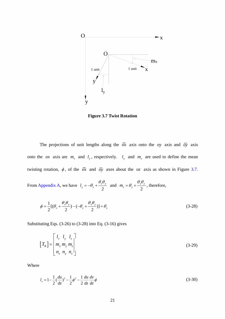
Figure 3.7 Twist Rotation
The projections of unit lengths along the ˆˆox axis onto the oy axis and ˆˆoy axis
onto the ox axis are xm and yl , respectively. yl and xm are used to define the mean
twisting rotation, φ , of the ˆˆox and ˆˆoy axes about the oz axis as shown in Figure 3.7.
From Appendix A, we have 2x y
y zlθ θ
θ= − + and 2x y
x zmθ θ
θ= + , therefore,
1 [( ) ( )]2 2 2
x y x yz z z
θ θ θ θφ θ θ θ= + − − + = (3-28)
Substituting Eqs. (3-26) to (3-28) into Eq. (3-16) gives
[ ]x y z
R x y z
x y z
l l lT m m m
n n n
=
(3-29)
Where
2 21 1 11 ( )
2 2 2xdu du dvldz dz dz
φ φ= − − − (3-30)
22
2 21 1 1( ) ( )
2 4 4ydu dv du dvldz dz dz dz
φ φ φ= − − + − (3-31)
z
duldz
= (3-32)
2 21 1 1( ) ( )
2 4 4xdu dv dv dumdz dz dz dz
φ φ φ= − − + (3-33)
2 21 1 11 ( )
2 2 2ydv du dvmdz dz dz
φ φ= − − + (3-34)
z
dvmdz
= (3-35)
21
4xdu dv dundz dz dz
φ φ= − − + (3-36)
21
4ydv du dvndz dz dz
φ φ= − + + (3-37)
2 21 11 ( ) ( )
2 2zdu dvndz dz
= − − (3-38)
The torsional curvature of the deformed cross section axes is (Love 1944)
x x x
z y y ydl dm dnk l m ndz dz dz
= + + (3-39)
Substituting Eqs. (3-30) to (3-38) into Eq. (3-39) gives
2 2
2 2
1 ( )2z
d d u dv d v dukdz dz dz dz dzφ
= + + (3-40)
The second and third term in this equation are small compared to the first term because of the
higher order effects. Eq. (3-40) may be approximated by
z
dkdzφ
= (3-41)
Substitue Eqs. (3-30) to (3-41) into Eq. (3-12), the displacement of an arbitrary point on the
cross section may be expressed in terms of the centroidal deformations as
23
ˆˆ
ˆˆ
p
p
p
u u yv v xw du dv dw x y
dz dz dz
φφ
φω
− = + − − −
+
2 2 2 2
2 2 2 2
2
1 1 1 1ˆˆ ( ) ( ) ( )2 2 2 21 1 1 1ˆˆ ( ) ( ) ( )2 2 2 2
1 1ˆ( ) (4 4
du du dv du dv du dv du dx ydz dz dz dz dz dz dz dz dz
du dv dv du dv du dv dv dx ydz dz dz dz dz dz dz dz dz
dv du du dvx ydz dz dz dz
φφ φ φ φ ω
φφ φ φ φ ω
φ φ φ φ
− + + − − + − − + − − + − −
− − + + 2 2 21) ( ) ( )2
d du dvdz dz dzφω
+ +
(3-42)
The first bracket on the right side of Eq. (3-42) contains the linear terms of the
displacements, and the second bracket contains the nonlinear terms of the displacements.
The derivatives of pu , pv , and pw with respect to z are
ˆ ( , , )p
x
du du d du dvydz dz dz dz dz
φ φ= − +Ο (3-43)
ˆ ( , , )p
y
dv dv d du dvxdz dz dz dz dz
φ φ= + +Ο (3-44)
2 2 2 2 2
2 2 2 2 2ˆˆˆˆˆˆ ( , , )pz
dw dw du d v d d dv d v d du d u du dvx y x x y ydz dz dz dz dz dz dz dz dz dz dz dz dz
φ φ φω φ φ φ= − − − − − + + +Ο
(3-45)
The terms xΟ and yΟ indicate functions of second and higher order in magnitude, and the
term zΟ indicates functions of third order and higher in magnitude, all of which are
disregarded.
24
3.1.3 Strains
The longitudinal finite normal strain may be expressed as (Boresi 1993)
2 2 21 [( ) ( ) ( ) ]
2P P P Pdw du dv dw
dz dz dz dzε = + + + (3-46)
Since Pdwdz
is small compared to Pdudz
and Pdvdz
, we can simplify this equation into
2 21 [( ) ( ) ]
2P P Pdw du dv
dz dz dzε = + + (3-47)
Substituting in the derivatives of the displacements of point oP from Eqs. (3-43) to (3-45),
Eq. (3-47) becomes
2 2 2 2 22 2 2 2 2
2 2 2 2 2
1 1ˆˆˆˆˆˆ [( ) ( ) ] ( )( )2 2P
dw d u d v d du dv d v d u dx y x y x ydz dz dz dz dz dz dz dz dz
φ φε ω φ φ= − − − + + − + + +
(3-48)
The first and second variations of the longitudinal strain are
2 2 2 2 2
2 2 2 2 2ˆˆˆˆPd w d u d v d d u du d v dv d v d vx y x xdz dz dz dz dz dz dz dz dz dzδ δ δ δφ δ δ δδε ω φ δφ= − − − + + − −
2 2
2 22 2ˆˆˆˆ ( )d u d u d dy y x y
dz dz dz dzδ δφ φφ δφ+ + + +
(3-49)
2 22 2 2 2 2 2
2 2ˆˆˆˆ( ) ( ) 2 2 ( )( )Pd u d v d v d u dx y x ydz dz dz dz dzδ δ δ δ δφδ ε δφ δφ= + − + + +
(3-50)
The second variations of the displacements in the above equations are assumed to
vanish.
25
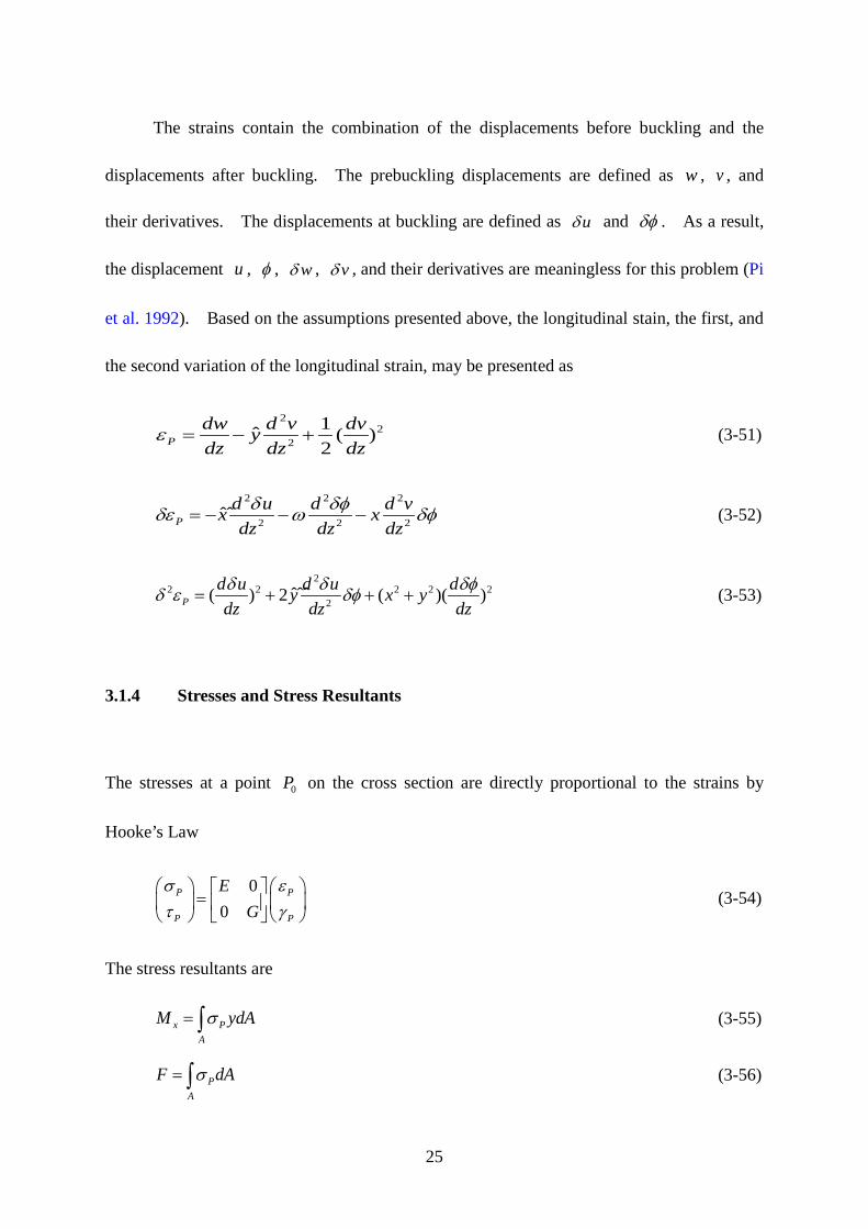
The strains contain the combination of the displacements before buckling and the
displacements after buckling. The prebuckling displacements are defined as w , v , and
their derivatives. The displacements at buckling are defined as uδ and δφ . As a result,
the displacement u , φ , wδ , vδ , and their derivatives are meaningless for this problem (Pi
et al. 1992). Based on the assumptions presented above, the longitudinal stain, the first, and
the second variation of the longitudinal strain, may be presented as
22
2
1ˆ ( )2P
dw d v dvydz dz dz
ε = − + (3-51)
2 2 2
2 2 2ˆˆPd u d d vx xdz dz dzδ δφδε ω δφ= − − − (3-52)
22 2 2 2 2
2ˆˆˆ( ) 2 ( )( )Pd u d u dy x ydz dz dzδ δ δφδ ε δφ= + + + (3-53)
3.1.4 Stresses and Stress Resultants
The stresses at a point 0P on the cross section are directly proportional to the strains by
Hooke’s Law
00
P P
P P
EG
σ ετ γ
=
(3-54)
The stress resultants are
x P
A
M ydAσ= ∫ (3-55)
P
A
F dAσ= ∫ (3-56)
26
3.1.5 Section Properties
For a member of length L with a doubly symmetric cross section, the x and y principal
centroidal axes are defined by
ˆˆ 0
A A
xdA ydA= =∫ ∫ (3-57)
ˆˆ 0
A
xydA =∫ (3-58)
The section properties are defined as
A
A dA= ∫ (3-59)
2ˆxA
I y dA= ∫ (3-60)
2ˆyA
I x dA= ∫ (3-61)
2ˆA
I dAω ω= ∫ (3-62)
24 PA
J t dA= ∫ (3-63)
The shear center of a doubly symmetric cross section coincides with the centroid, which
satisfies the conditions
ˆ 0
A
x dAω =∫ (3-64)
ˆ 0
A
y dAω =∫ (3-65)
0
A
dAω =∫ (3-66)
27
3.1.6 Strain Energy Equation
The second variation of the strain energy equation is developed by substituting Pε , Pδε ,
2Pδ ε , Pγ , Pδγ , and 2
Pδ γ along with the stresses, stress resultants, and section properties
from Sections 3.1.2 and 3.1.3 into Eq. (3-6). The second variation of the strain energy for
the flexural-torsional buckling problem is
2 2 22 2 2 2
2 2 2
1 1 ( ) ( ) ( ) ( )[ ( ) ( ) ( ) 2 ( )2 2 y x
d u d d d uU EI EI GJ Mdz dz dz dzωδ δφ δφ δδ δφ= + + +∫
2( )( ) ]d uF dz
dzδ
+
(3-67)
Where the stress resultants are linearized to
2
2x xd vM EIdz
= − (3-68)
dwF EAdz
= (3-69)
3.2 POTENTIAL ENERGY OF THE LOADS
The second part of the total potential energy equation, Eq. (3-1), is the potential energy of the
external loads, may be expressed by the multiplication of the external loads with the
corresponding displacements:
28
( ) ( )M
q p FL
dvv q dz v P M w Fdz
Ω = − −∑ − +∫ (3-70)
where
qv = vertical displacement through which the load q acts
q = the distributed load in the y - direction
pv = vertical displacement through which the load P acts
P = the concentrated load in the y - direction
Mv = vertical displacement through which the moment M acts
Mdv
dz = rotation due to the moment M
M = the applied moment about the x - axis
Fw = longitudinal displacement through which the load F acts
F = the concentrated load in the z - direction
The second variation of the potential energy of the loads is
22 2 2 2( ) ( )M
q p FL
d vv q dz v P M w Fdzδδ δ δ δΩ = − −∑ − +∫ (3-71)
29
3.2.1 Displacements
The longitudinal displacement is considered negligible due to its small quantity, therefore,
0Fw = . The displacement due to the concentrated load P at a height of ze from the
neutral axis may be found by using Eq. (3-42) ( 0, , 0)zx y e ω= = =
P y z zv v m e e= + − (3-72)
Substituting Eq. (3-34) into Eq. (3-72) gives
2 21 [( ) ]
2P zdv du dvv v edz dz dz
φ φ= − + − (3-73)
Likewise, the displacement due to the distributed load is
2 21 [( ) ]
2q zdv du dvv v adz dz dz
φ φ= − + − (3-74)
Also, the rotation about an axis parallel to the ox axis at a point with a concentrated moment
xM is
Mdv dv
dz dz= (3-75)
In this section, the effects of prebuckling deformations are neglected; therefore, the
deformation v and its derivatives are disregarded. The displacements corresponding to the
external loads become
21
2q zv a φ= (3-76)
21
2P zv e φ= − (3-77)
0Mdv
dz= (3-78)
30
The second variations of Eqs. (3-76) to (3-78) are
2 2( )q zv aδ δφ= (3-79)
2 2( )P zv eδ δφ= (3-80)
2
0Md vdzδ
= (3-81)
3.2.2 Potential Energy of Loads Equation
Substituting in the displacements of Eqs. (3-79) to (3-81) into Eq. (3-71) gives the second
variation of the potential energy of the loads
2 2 21 1 1( ) ( )2 2 2z z
L
qa dz Peδ δφ δφΩ = + ∑∫ (3-82)
3.3 ENERGY EQUATION
The second variation of the total potential energy equation for the flexural-torsional buckling
of a beam element is the sum of the second variation of the strain energy and the second
variation of the potential energy of the loads. Therefore, the second variation of the total
potential energy equation is given by
31
2 2 22 2 2 2 2
2 2 2
1 1 ( ) ( ) ( ) ( ) ( )( ) ( ) ( ) 2 ( ) ( ) ]2 2 y x
d u d d d u d uEI EI GJ M F dzdz dz dz dz dzωδ δφ δφ δ δδ δφ
∏ = + + + +
∫
2 21 1( ) ( ) 02 2z z
L
qa dz Peδφ δφ+ + ∑ =∫ (3-83)
Where
2
1 1 2xzM M V z q= + − for 0 Pz z< < (3-84)
2
1 1 ( )2x PzM M V z q P z z= + − − − for Pz z L< < (3-85)
Pz = the location where the concentrated load applies.
32
4.0 DERIVATION OF SECTION PROPERTIES OF A DOUBLY-SYMMETRIC
WEB-TAPERED I-BEAM
In uniform beams, calculation of the section properties such as cross section area, A , the
second moment of inertia, xI or yI , the torsional constant, J , and etc., are standard
procedure and can easily be determined from the characteristics of the cross section.
However, because of the tapered effects, these calculations are more complex for a
web-tapered I-beam. These section properties are changed along the length, and they are
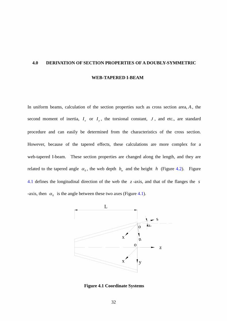
related to the tapered angle 0α , the web depth wb and the height h (Figure 4.2). Figure
4.1 defines the longitudinal direction of the web the z -axis, and that of the flanges the s
-axis, then 0α is the angle between these two axes (Figure 4.1).
L
x y
z
o
nx
sα0
o
Figure 4.1 Coordinate Systems
33
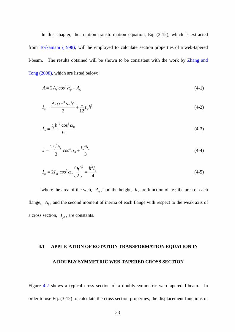
In this chapter, the rotation transformation equation, Eq. (3-12), which is extracted
from Torkamani (1998), will be employed to calculate section properties of a web-tapered
I-beam. The results obtained will be shown to be consistent with the work by Zhang and
Tong (2008), which are listed below:
3
02 cosf wA A Aα= + (4-1)
3 20 3cos 1
2 12f
x w
A hI t h
α= + (4-2)
3 30cos
6f f
y
t bI
α= (4-3)
3 33
0
2cos
3 3f f w wt b t bJ α= + (4-4)
0
2 232 cos
2 4y
yf
h IhI Iω α = =
(4-5)
where the area of the web, wA , and the height, h , are function of z ; the area of each
flange, fA , and the second moment of inertia of each flange with respect to the weak axis of
a cross section, yfI , are constants.
4.1 APPLICATION OF ROTATION TRANSFORMATION EQUATION IN
A DOUBLY-SYMMETRIC WEB-TAPERED CROSS SECTION
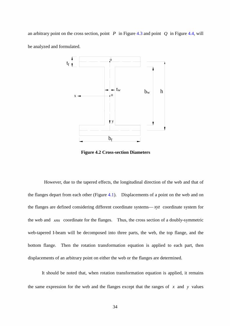
Figure 4.2 shows a typical cross section of a doubly-symmetric web-tapered I-beam. In
order to use Eq. (3-12) to calculate the cross section properties, the displacement functions of
34
an arbitrary point on the cross section, point P in Figure 4.3 and point Q in Figure 4.4, will
be analyzed and formulated.
bf
x
y
o
o
tw
tf
bw h
Figure 4.2 Cross-section Diameters
However, due to the tapered effects, the longitudinal direction of the web and that of
the flanges depart from each other (Figure 4.1). Displacements of a point on the web and on
the flanges are defined considering different coordinate systems— xyz coordinate system for
the web and xns coordinate for the flanges. Thus, the cross section of a doubly-symmetric
web-tapered I-beam will be decomposed into three parts, the web, the top flange, and the
bottom flange. Then the rotation transformation equation is applied to each part, then
displacements of an arbitrary point on either the web or the flanges are determined.
It should be noted that, when rotation transformation equation is applied, it remains
the same expression for the web and the flanges except that the ranges of x and y values
35
are changed, which are discussed in this section. Then, by employing the finite normal strain,
the section properties are derived for five different cases.
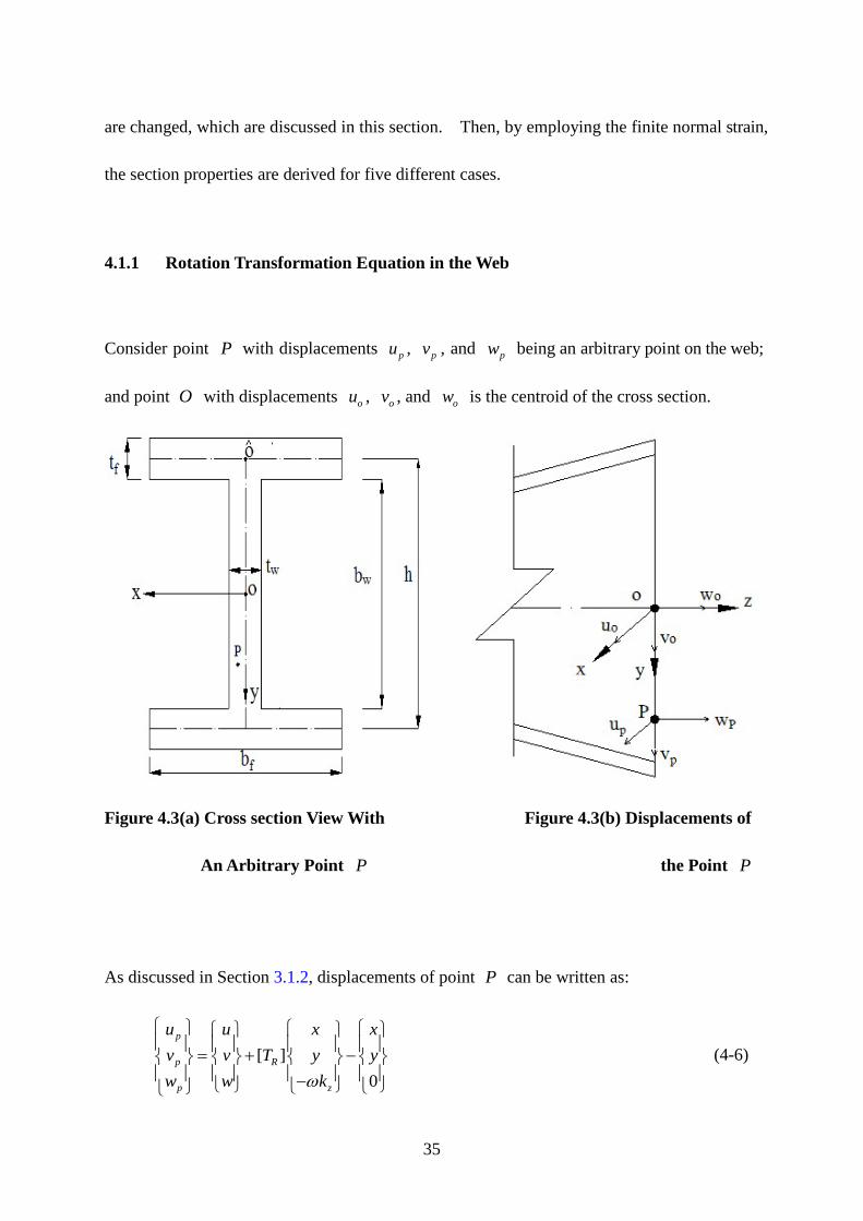
4.1.1 Rotation Transformation Equation in the Web
Consider point P with displacements pu , pv , and pw being an arbitrary point on the web;
and point O with displacements ou , ov , and ow is the centroid of the cross section.
Figure 4.3(a) Cross section View With Figure 4.3(b) Displacements of
An Arbitrary Point P the Point P
As discussed in Section 3.1.2, displacements of point P can be written as:
[ ]0
p
p R
p z
u u x xv v T y yw w kω
= + − −
(4-6)
36
where the values of x and y are bounded as given below:
2 2w wt tx− ≤ ≤ (4-7)
2 2w wb by≤ ≤ − (4-8)
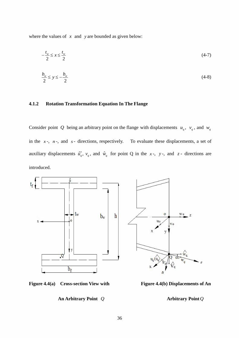
4.1.2 Rotation Transformation Equation In The Flange
Consider point Q being an arbitrary point on the flange with displacements qu , qv , and qw
in the x -, n -, and s - directions, respectively. To evaluate these displacements, a set of
auxiliary displacements ˆˆ , q qu v , and ˆ qw for point Q in the x -, y -, and z - directions are
introduced.
Figure 4.4(a) Cross-section View with Figure 4.4(b) Displacements of An
An Arbitrary Point Q Arbitrary Point Q
37
The displacement functions for ˆˆ , q qu v , and ˆ qw can be written as:
ˆˆ [ ]ˆ 0
q
q R
q z
u u x xv v T y yw w kω
= + − −
(4-9)
Displacements qu , qv , and qw are calculated in terms of displacements ˆˆ , q qu v , ˆ qw ,
and angle 0α considering geometry of the cross section (See Figure 4.4b). For both the top
and the bottom flange, one may have:
^
q qu u= (4-10)
^ ^
0 0cos sinqq qv v wα α= + (4-11)
^ ^
0 0cos sinqq qw w vα α= − (4-12)
Eqs. (4-10) to (4-12) may be expressed in matrix form:
[ ]0 0
0 0
ˆˆ1 0 0ˆˆ0 cos sinˆˆ0 sin cos
q q q
q q q
q q q
u u uv v T vw w w
α αα α
= =
−
(4-13)
Where
[ ] 0 0
0 0
1 0 00 cos sin0 sin cos
T α αα α
= −
(4-14)
Substituting Eq. (4-9) into the right-hand side of Eq. (4-13), one has displacements of an
arbitrary point Q on the flange:
38
[ ] [ ]ˆˆ [ ]ˆ 0
q q
q q R
q q z
u u u x xv T v T v T y yw w w kω
= = + −
−
(4-15)
where the values of x and y are bounded and are given by the equations below.
For the top flange:
2 2f fb b
x− ≤ ≤ (4-16)
2 2 2 2f ft th hy− − ≤ ≤ − + (4-17)
For the bottom flange:
2 2f fb b
x− ≤ ≤
(4-18)
2 2 2 2f ft th hy− ≤ ≤ + (4-19)
4.2 FINITE NORMAL STRAIN
Finite normal strain is a well defined concept, only the longitudinal finite normal strain is used
in this work. After the displacements have been obtained for an arbitrary point on both the
web and the flanges, the longitudinal finite normal strain can be employed to define the strains.
For point P on the web, the longitudinal normal finite strain is:
2 2 2
p1 [( ) ( ) ( ) ]2
p p p pdw du dv dwdz dz dz dz
ε = + + + (4-20)
39
For point Q on the flanges, the longitudinal normal finite strain is:
2 2 2
q1 [( ) ( ) ( ) ]2
q q q qdw du dv dwds ds ds ds
ε = + + + (4-21)
where
0cosdz
dsα= (4-22)
4.3 DERIVATION OF SECTION PROPERTIES
In this section, several well defined deformation patterns are investigated, and the
corresponding section properties of a doubly-symmetric web-tapered I-beam are derived.
This is done based on the formulations presented in the previous sections.
4.3.1 Axial Deformation
When displacement in z − direction is the only displacement, one has no rotation, thus 0θ = ,
then 0x y zθ θ θ= = = ; from Eq.(3-16), ( cos ) 0zd dkdz dzφ θ γ
= = = ; the displacements of the
centroid are 0u v= = , and 0w ≠ . From Eq. (3-13), one has
[ ]1 0 00 1 00 0 1
RT =
(4-23)
40
4.3.1.1 Axis deformation of the web
The displacements of point P on the web in terms of centroidal displacement are given by
Eq. (4-6),
0[ ] 0
0 0
p
p R
p
u u x xv v T y yw w w
= + − =
(4-24)
From Eq. (4-20), we can express the strain of point P as
' 2 ' '2
p1 10 0 ( )2 2
pp
dww w w
dzε = + + + = + (4-25)
If the higher order term is disregarded, the linear term is:
'
pL wε = (4-26)
The corresponding axial force on the web is
'L
w w w P w wN t dy E t dy Ew Aσ ε= = =∫ ∫ (4-27)
4.3.1.2 Axial deformation of the flange
First, we need to find ˆˆ, q qu v , and ˆ qw using Eq. (4-9),
ˆ 0ˆ [ ] 0ˆ 0 0
q
q R
q
u u x xv v T y yw w w
= + − =
(4-28)
41
Then qu , qv , and qw are calculated using Eq. (4-13)
0 0 0
0 0 0
ˆ1 0 0 0ˆ0 cos sin sinˆ0 sin cos cos
q q
q q
q q
u uv v ww w w
α α αα α α
= =
−
(4-29)
The normal strain is calculated using Eq. (4-21):
2 2 2q
1 0 ( ) ( )2
q q qdw dv dwds ds ds
ε
= + + +
' 2 2 ' 2 20 0 0 0
1cos [( sin cos ) ( cos ) ]2
w w wα α α α= + + (4-30)
The nonlinear terms in Eq. (4-30) show that the deformation in the flange is a curve due to the
axial deformation in the web. For simplicity, only the linear terms are kept:
' 2
q 0cosL wε α= . (4-31)
The corresponding axial force in the s -direction on the flange is
' 2
, 0cosLf s f q fN EA EA wε α= = . (4-32)
The component of ,f sN in the z -direction is
' 3
, , 0 0cos cosf z f s fN N EA wα α= = . (4-33)
4.3.1.3 Derivation of the cross section area
If one sums up the forces in z -direction using Eqs. (4-27) and (4-33), the axial force of the
whole cross section in the z -direction can be determined:
42
,2 f z wN N N= +
' 30(2 cos )f wEw A Aα= + (4-34)
Thus, the effective cross-section area is
3
02 cosf wA A Aα= + . (4-35)
4.3.2 Bending about x -axis
When rotation about x -axis is the only displacement, one has
' , 0, 9 0 ;ovθ α β γ= = = =
'cosx vθ θ α= = , cos 0yθ θ β= = , cos 0zθ φ θ γ= = = ;
/ 0zk d dzφ= = ;
0u v w= = = . (4-36)
Substituting Eq. (4-36) into Eq. (3-13), we have
[ ]'2
'
'2'
1 00
0 12
0 12
RvT v
vv
= − − −
(4-37)
43
4.3.2.1 Bending about x –axis of the web
Using Eq. (3-12), we have:
'2 '2
' '
0(1 / 2 ) / 2
p
p
p
u u x xv v v y y v yw v y w v y
+ − = + − − = − +
. (4-38)
Then from Eq. (4-20):
2 2 2p
1 0 ( ) ( )2
p p pdw dv dwdz dz dz
ε
= + + +
'' '' ' 2 '' 21 ( ) ( )2
v y v v y v y = + + (4-39)
When linear terms are kept:
''L
P v yε = . (4-40)
Thus, the moment about x -axis considering only the web may be calculated
3"
12L
w w w w wp
hM yt dy E yt dy Ev tσ ε= = =∫ ∫ (4-41)
4.3.2.2 Bending about x –axis of the flanges
First, we need to find ˆˆ, q qu v , and ˆ qw using Eq. (3-12)
'2'
'2'
1 00ˆˆ 0 1
2ˆ 0 0
0 12
q
q
q
x xu uvv v v y y
w w vv
= + − − −
−
'2
'
0/ 2v y
yv
= −
(4-42)
44
Then from Eq. (4-13), we get:
' '20 0 0 0
' '20 0 0 0
ˆ1 0 0 0ˆ0 cos sin sin cos / 2ˆ0 sin cos cos sin / 2
q q
q q
q q
u uv v yv v yw w yv v y
α α α αα α α α
= = −
− +
(4-43)
Using Eq. (4-21) to determine the normal strain:
2 2 2q,s
1 ( ) ( ) ( )2
q q q qdw du dv dwds ds ds ds
ε
= + + +
" 2 ' " " ' " 2 20 0 0 0 0 0
1cos sin cos ( sin cos cos )2
yv v v y yv v v yα α α α α α= + + −
" 2 ' " 20 0 0
1 ( cos sin cos )2
yv v v yα α α+ + (4-44)
When linear terms are kept:
" 2
q,s 0cosL yvε α= . (4-45)
Then, the axial forces in the top and the bottom flange are obtained based on Eqs. (4-16) to
(4-19):
For the top flange:
2 2
, 1 , 1 , 12 2
f
f
thL L
tf s f f s f s fhN EA E b dyε ε− +
− −= = ∫ .
" 20
1 cos2 fEv Aα= − (4-46)
Likewise, for the bottom flange:
2 2
, 2 , 2 , 22 2
f
f
thL L
tf s f f s f s fhN EA E b dyε ε+
−= = ∫
45
" 20
1 cos2 fEv Aα= . (4-47)
4.3.2.3 Derivation of the moment of inertia about the x -axis
The moment of the whole cross-section about x -axis can be derived using Eqs. (4-41), (4-46)
and (4-47):
, 2 0 , 1 0cos cos
2 2x f s f s wh hM N N Mα α= − +
2
" 3 30
1( cos )2 12f
w
A hEv t hα= + . (4-48)
From standard moment-curvature relations
23 3
01( cos )
2 12f
x w
A hI t hα= + . (4-49)
4.3.3 Bending about y -axis
When rotation about y -axis is the only displacement, one has,
0' 0, 90 , 0uθ α γ β= = = = ;
cos 0xθ θ α= = , 'cosy uθ θ β= = , cos 0zθ θ γ= = ;
/ / 0z zk d dz d dzφ θ= = = ;
0u v w= = = . (4-50)
46
4.3.3.1 Bending about the y –axis of the web
The moment about the weak axis in the web is relatively small compared to the moment in the
flanges, thus, it is neglected here.
4.3.3.2 Bending about the y –axis of the flanges
Substituting Eq. (4-50) into Eq. (3-13), we get
[ ]
'2
'2'
1 0 '2
0 1 0
0 12
R
u u
Tuu
−
= − −
(4-51)
We need to find ˆˆ, q qu v , and ˆ qw first using Eq. (3-12):
'2
'2'
1 0 'ˆ 2ˆ 0 1 0ˆ 0 0
0 12
q
q
q
u uu u x xv v y yw w uu
− = + −
− −
'2
'
20
u x
u x
= −
(4-52)
Using Eq. (4-13), we get:
'2
'0 0 0
'0 0 0
ˆ1 0 0 / 2ˆ0 cos sin sinˆ0 sin cos cos
q q
q q
q q
u u u xv v u xw w u x
α α αα α α
− = = −
− −
(4-53)
47
From Eq. (4-21), we can have:
2 2 2q,s
1 ( ) ( ) ( )2
q q q qdw du dv dwds ds ds ds
ε
= + + +
" ' " 2 " 2 20 0 0
1cos ( cos ) ( cos )2
u x u u x u xα α α = − + + (4-54)
When only the linear terms are kept:
"
q,s 0cosL u xε α= − . (4-55)
Thus, the moment of the bottom flange about the n -axis can be determined:
/2
, 2 ,/2
f
f
b Lf n q s fb
M E xt dxε−
= ∫
" 2 30
1cos12 f fEu b tα= . (4-56)
Likewise, for the top flange, we have:
" 2 3
, 1 01cos
12f n f fM Eu b tα= . (4-57)
4.3.3.3 Derivation of the moment of inertia about the y -axis
Finally, the bending moment of the whole cross section about the y -axis can be determined by
combining Eqs. (4-56) and (4-57):
, 1 0 , 2 0cos cosy f n f nM M Mα α= +
" 3 3
01cos6 f fEu b tα= "
yEu I= (4-58)
Where 3 30
1cos6y f fI b tα= (4-59)
48
4.3.4 Free Torsional Deformation
In this case, there is a pure twist about the z -axis in the cross section, the twisting angle is zθ .
00, 90 , 0θ θ α β γ= = = = ;
cos 0xθ θ α= = , cos 0yθ θ β= = , coszθ θ γ θ= = ;
'/ /z zk d dz d dzφ θ θ= = = ;
0u v w= = = . (4-60)
Substituting Eq. (4-60) into Eq. (3-13), we get
[ ]
2
2
1 / 2 0
1 / 2 0
0 0 1
RT
θ θ
θ θ
− −
= −
(4-61)
4.3.4.1 Torsional deformation of the web
The twist of the web about the z -axis is zθ θ= , from the classical thin-walled theory
developed by Vlasov (1961), the resultant free torsional torque is given by
w w
dT GJdzθ
= (4-62)
Where
3 / 3w w wJ b t= (4-63)
49
4.3.4.2 Torsional deformation of the flanges
The twisting angle of the top flange about the 1s -direction is
1 cossθ θ α= (4-64)
Then the corresponding twist is obtained
' 21
1
cossddsθ θ α= (4-65)
The resultant free torsional torque of the top flange with respect to the 1s -direction is given by
1
1 1
',
2
1
coss ff s f
dGJ
dJ
sT G
θθ α== (4-66)
where 3 / 3 f ffJ t b= (4-67)
Likewise, one may have the expression for the bottom flange.
2
2 2
',
2
2
coss ff s f
dGJ
dJ
sT G
θθ α== (4-68)
4.3.4.2 Derivation of torsional constant
Finally, using Eqs. (4-66) and (4-68), one may express the torque of the whole cross section
about the z -axis
1 2 1 2, , , 1 , 2 0( ) cosf z f z w f s f s wT T T T T T Tα= + + = + +
' 3 '
02 cosf wGJ GJθ α θ= + ' 30(2 cos )f wG J Jθ α= + (4-69)
50
Where we find the equivalent free torsional constant of the cross-section
3 33 3
0 0
22 cos cos
3 3f f w w
f w
b t b tJ J Jα α= + = + (4-70)
4.3.5 Warping Strain of the Flanges Due to Free Torsional Deformation
4.3.5.1 Warping strain of the top flange in 1s -direction
Due to the assumption of zero linear shear strain on the middle surface of the top flange:
1
1
0ssx
w ux s
γ∂ ∂
= + =∂ ∂
(4-71)
1sw and u are the displacements of an arbitrary point on the middle surface of the top flange
along the 1s - and x -axis, respectively.
To get u , set 2hy = − in Eq. (3-13) using Eqs. (4-60) and (4-61), and make the
differentiation with respect to the 1s -axis, we will obtain
2 / 2
2hu xθ θ= − (4-72)
' '0 0 0 0
1
cos cos ( tan ) cos2
u hu xs
α α θ α θ θθ α∂= = + −
∂ (4-73)
Then we can write the expression for 1sw from Eq. (4-71)
51
'' 2
1 0 0 0 0tan cos cos cos / 22s
hw x x xθθ α α α θθ α
= − + −
=' '
20 0 0sin cos cos
2 2hx x xθ θθθ α α α
− + −
(4-74)
Neglecting the nonlinear terms in Eq. (4-21), the linear term of the strain can be determined
'1, 1 1 0
1
cosL sf s s
dw wds
ε α= =
"
' 20 0( 2 tan )cos
2hx θ θ α α= − + (4-75)
The bending moment of the top flange about the 1n -axis is given by:
/ 2
, 1 ,/ 2
f
f
b Lf n f s fb
M E xt dxε−
= ∫
" / 22 ' 2
0 0 / 2cos ( 2 tan )
2f
f
b
b
hE x dxθα θ α−
= − + ∫
"
2 '0 0cos ( 2 tan )
2yfhEI θα θ α= − + . (4-76)
The shear force along the x -axis due to the warping is thus determined:
, 1 ', 1 1, 1 0
1
cosn ff n n f
dMQ M
dsα= =
"'
3 "0 0cos ( 3 tan )
2yfhEI θα θ α= − + (4-77)
52
4.3.5.2 Warping strain of the top flange in 2s -direction
Likewise, the shear force along the bottom flange can also be analyzed using the same
procedure, which is listed with the other parameters as below:
'
2 0 0( tan )cos2s
hw x θ θ α α= + (4-78)
"' 2
, 2 0 0( 2 tan )cos2
Lf s
hx θε θ α α= + (4-79)
"2 '
2, 1 0 0cos ( 2 tan )2f n yf
hM EI θα θ α= + (4-80)
"'3 "
2, 1 0 0cos ( 3 tan )2f n yf
hQ EI θα θ α= + . (4-81)
4.3.5.3 Derivation of the warping constant
Finally, the bi-moment of the cross-section can be evaluated using Eqs. (4-76) and (4-80)
1 1 2 20 , ,cos ( )2w n f n fhB M Mα= −
3 " ' ' '0 0cos ( / 2 2 tan ) ( )yf whEI h E Iα θ θ α θ= − + = − (4-82)
where 3 202 cos ( )
2w yfhI I α= (4-83)
53
4.4 CONCLUSION
By investigating five deformation cases, the rotation transformation equation is used to derive
the displacements and strains for an arbitrary point in the cross section of a doubly-symmetric
web-tapered I-beam. It has been shown that the results of the section properties have a good
agreement with Tong and Zhang (2003a), which demonstrates the efficiency as well as the
accuracy of the rotation transformation equation in analyzing a web-tapered I-beam problem.
The normal finite strain is truncated in this derivation process, depending upon desire
accuracy, some of the nonlinear terms may be considered in calculations if required.
54
5.0 FINITE ELEMENT METHOD
The finite element analysis is a powerful numerical method to solve problems in many
engineering fields and mathematical physics. Since the analytical solutions to many cases
are difficult to obtain due to complicated geometries, loadings and material properties, the
finite element method, which requires the solution of a system of simultaneous equations
rather than complicated differential equations, provides a much easier way to generate results
within acceptable errors.
The general steps to formulate the finite element solution begin with discretizing the
structure into smaller elements. After this, the type for each element must be selected, and it
should be chosen to closely model the actual behavior of the real body. Next, a
displacement function is assumed for each element. The most common displacement
function is a polynomial function expressed in terms of the nodal unknowns. The total
number of polynomial functions needed to describe the displacement of an element depends
on the number of degrees of freedom of the element. The strain-displacement relationship
and stress-strain relationship are then defined for each element. These relationships are
necessary to derive equations describing each element’s behavior.

55
Equivalent loads at each node of the element need to be defined. Then the element
stiffness matrices may be derived using one of several methods including energy methods as
used in this Chapter. It should be noted that, unlike other energy methods such as the
principle of virtual work, the principle of minimum total potential energy is applicable only
for elastic materials. In this paper, the element stiffness matrices for flexural-torsional
buckling of a beam element, including the elastic stiffness matrix and the geometric stiffness
matrix, will be produced using principle of minimum total potential energy.
After the element stiffness matrices are derived, the element matrices will be
converted from the local to global coordinate system for the entire structure using
transformation matrix. Then through the assembly process, the governing equation for the
whole structure can be obtained. The global stiffness matrix will be singular when there are
no boundary conditions applied to the structure. In order to remove the singularity, the
boundary conditions are applied to the matrix so that the structure does not move as a rigid
body. This process involves partitioning the global matrix into the free and restrained
degrees of freedom. The section of the global stiffness matrix corresponding to the free
degrees of freedom of the structure is used for solving the problem. For the
flexural-torsional buckling problem, the partitioned global elastic and geometric stiffness
matrices are used to solve for the buckling loads.
In this paper, the objective is to apply the finite element method to a doubly-symmetric
web-tapered I-beam to calculate the flexural-torsional buckling load of the structure.
56
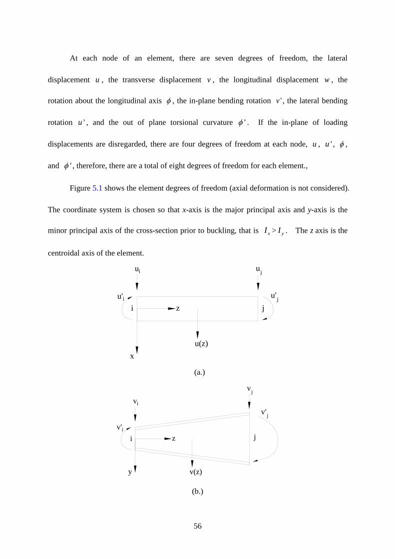
At each node of an element, there are seven degrees of freedom, the lateral
displacement u , the transverse displacement v , the longitudinal displacement w , the
rotation about the longitudinal axis φ , the in-plane bending rotation 'v , the lateral bending
rotation 'u , and the out of plane torsional curvature 'φ . If the in-plane of loading
displacements are disregarded, there are four degrees of freedom at each node, u , 'u , φ ,
and 'φ , therefore, there are a total of eight degrees of freedom for each element.,
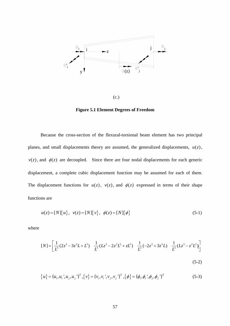
Figure 5.1 shows the element degrees of freedom (axial deformation is not considered).
The coordinate system is chosen so that x-axis is the major principal axis and y-axis is the
minor principal axis of the cross-section prior to buckling, that is xI > yI . The z axis is the
centroidal axis of the element.
x
z
u(z)
u'i
ji
u'ji j
(a.)
y
zv'i
vj
vi
v'j
v(z)
ji
(b.)
57
y
z
'i 'j(z)
ji ji
(c.)
Figure 5.1 Element Degrees of Freedom
Because the cross-section of the flexural-torsional beam element has two principal
planes, and small displacements theory are assumed, the generalized displacements, ( )u z ,
( )v z , and ( )zφ are decoupled. Since there are four nodal displacements for each generic
displacement, a complete cubic displacement function may be assumed for each of them.
The displacement functions for ( )u z , ( )v z , and ( )zφ expressed in terms of their shape
functions are
( ) [ ]u z N u= , ( ) [ ]v z N v= , ( ) [ ]z Nφ φ= (5-1)
where
3 2 3 3 2 2 3 3 2 3 2 2
3 3 3 3
1 1 1 1[ ] (2 3 ) ( 2 ) ( 2 3 ) ( )N z z L L Lz z L zL z z L Lz z LL L L L = − + − + − + −
(5-2)
, ', , 'Ti i j ju u u u u= , , ', , 'T
i i j jv v v v v= , , ', , 'Ti i j jφ φ φ φ φ= (5-3)
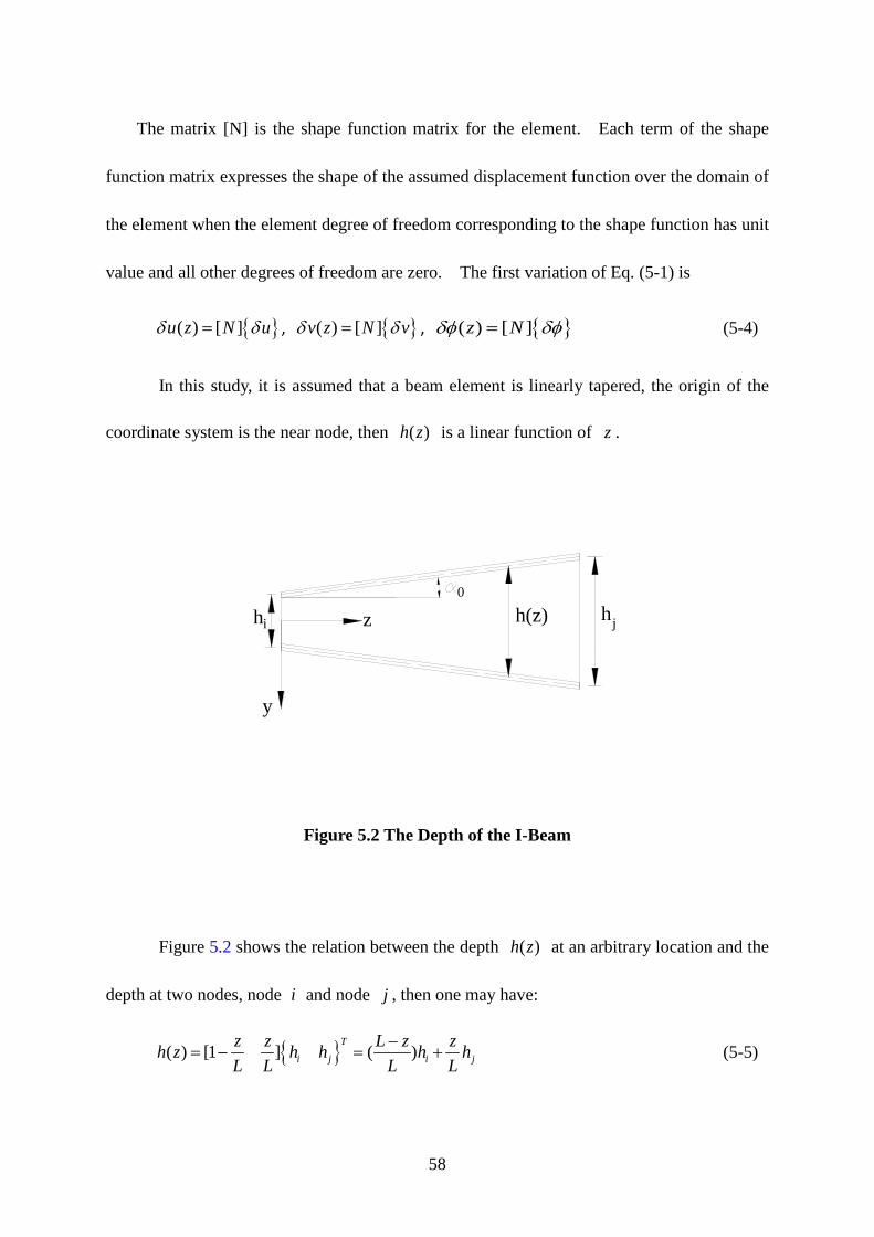
58
The matrix [N] is the shape function matrix for the element. Each term of the shape
function matrix expresses the shape of the assumed displacement function over the domain of
the element when the element degree of freedom corresponding to the shape function has unit
value and all other degrees of freedom are zero. The first variation of Eq. (5-1) is
( ) [ ]u z N uδ δ= , ( ) [ ]v z N vδ δ= , ( ) [ ]z Nδφ δφ= (5-4)
In this study, it is assumed that a beam element is linearly tapered, the origin of the
coordinate system is the near node, then ( )h z is a linear function of z .
y
z h(z)0
hjhi
Figure 5.2 The Depth of the I-Beam
Figure 5.2 shows the relation between the depth ( )h z at an arbitrary location and the
depth at two nodes, node i and node j , then one may have:
( ) [1 ] ( )
T
i j i jz z L z zh z h h h hL L L L
−= − = + (5-5)
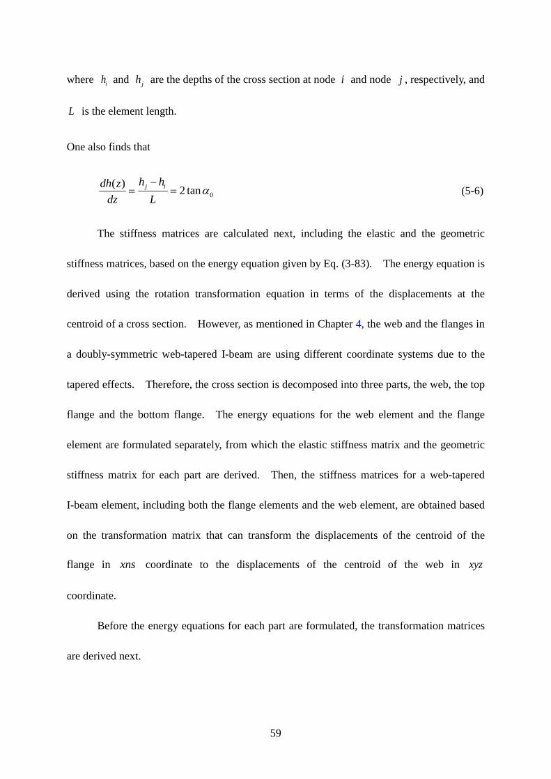
59
where ih and jh are the depths of the cross section at node i and node j , respectively, and
L is the element length.
One also finds that
0
( ) 2 tanj ih hdh zdz L
α−
= = (5-6)
The stiffness matrices are calculated next, including the elastic and the geometric
stiffness matrices, based on the energy equation given by Eq. (3-83). The energy equation is
derived using the rotation transformation equation in terms of the displacements at the
centroid of a cross section. However, as mentioned in Chapter 4, the web and the flanges in
a doubly-symmetric web-tapered I-beam are using different coordinate systems due to the
tapered effects. Therefore, the cross section is decomposed into three parts, the web, the top
flange and the bottom flange. The energy equations for the web element and the flange
element are formulated separately, from which the elastic stiffness matrix and the geometric
stiffness matrix for each part are derived. Then, the stiffness matrices for a web-tapered
I-beam element, including both the flange elements and the web element, are obtained based
on the transformation matrix that can transform the displacements of the centroid of the
flange in xns
coordinate to the displacements of the centroid of the web in xyz
coordinate.
Before the energy equations for each part are formulated, the transformation matrices
are derived next.
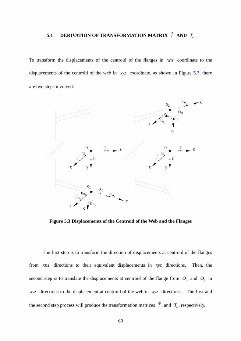
60
5.1 DERIVATION OF TRANSFORMATION MATRIX T AND eT
To transform the displacements of the centroid of the flanges in xns
coordinate to the
displacements of the centroid of the web in xyz coordinate, as shown in Figure 5.3, there
are two steps involved.
x y
z
o1
n
uu'
sx
uoα0
o
y
zo
1
'
u'o1
'o1
o1
o2
n
s
x
uo2'o
α0
2u'
o2
o2
x
uu''
Figure 5.3 Displacements of the Centroid of the Web and the Flanges
The first step is to transform the direction of displacements at centroid of the flanges
from xns
directions to their equivalent displacements in xyz directions. Then, the
second step is to translate the displacements at centroid of the flange from 1O , and 2O in
xyz directions to the displacement at centroid of the web in xyz directions. The first and
the second step process will produce the transformation matrices T , and eT , respectively.
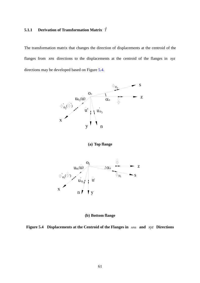
61
5.1.1 Derivation of Transformation Matrix T
The transformation matrix that changes the direction of displacements at the centroid of the
flanges from xns directions to the displacements at the centroid of the flanges in xyz
directions may be developed based on Figure 5.4.
o2
n
s
x
uo2
'o
α0
2 u'o2
o2
z
y
u'
(u)
( ')
(a) Top flange
o1
x
uo
'o
z
y
u'
(u)
( ') o
α0
u'o1
1
n
s1
1
(b) Bottom flange
Figure 5.4 Displacements at the Centroid of the Flanges in xns and xyz Directions
62
From the Figure 5.4, one may have:
For the top flange:
2ˆou u= (5-7)
2
'0 0
ˆˆ 'cos sinou u α φ α= + (5-8)
2 0 0ˆˆ 'sin coso uφ α φ α= − + (5-9)
2
' ˆ 'oφ φ= (5-10)
One may rewrite Eqs.(5-7) to (5-10) in the matrix form
2
2
2
2
'0 0
0 0
'
ˆ1 0 0 0ˆ '0 cos sin 0ˆ0 sin cos 0ˆ0 0 0 1 '
o
o
o
o
u uuu α α
φ α α φ
φ φ
= −
(5-11)
For the bottom flange:
1ˆou u= (5-12)
1
'0 0
ˆˆ 'cos sinou u α φ α= − (5-13)
1 0 0ˆˆ 'sin coso uφ α φ α= + (5-14)
1
' ˆ 'oφ φ= (5-15)
63
One may rewrite Eqs.(5-12) to (5-15) in the matrix form
1
1
1
1
'0 0
0 0
'
ˆ1 0 0 0ˆ '0 cos sin 0ˆ0 sin cos 0ˆ0 0 0 1 '
o
o
o
o
u uuu α α
φ α α φ
φ φ
− =
(5-16)
Eqs. (5-11) and (5-16) applies to the transformation of displacements at the top and
bottom flanges at node i . If we expand the matrices to an element including both nodes i
and j , the transformation matrix T for the top and bottom flanges are obtained.
For the top flange, based on Eq. (5-11), one has:
0
0 0
0 0
0
0 0
1 0 0 0 0 0 0 00 0 0 0 0 00 0 0 0 0 00 0 0 1 0 0 0 0ˆ( )0 0 0 0 1 0 0 00 0
cos sinsin cos
cos0 0 0 sin 00 0 0 0 0 sin 00 0 0
c0 0 0 0 1
os
topT
αα
α αα α
αα
− = −
(5-17a)
For the bottom flange, based on Eq. (5-16), one may have:
0 0
0 0
0
0
0
0
1 0 0 0 0 0 0 00 0 0 0 0 00 0 0 0 0 00 0 0 1 0 0 0 0ˆ( )0 0 0 0 1 0 0 00 0 0 0 0 sin 00 0 0 0 0 si
cos sinsin cos
coscosn 0
0 0 0 0 0 0 0 1
bottomT
αα
α αα α
αα
=
−
−
(5-17b)
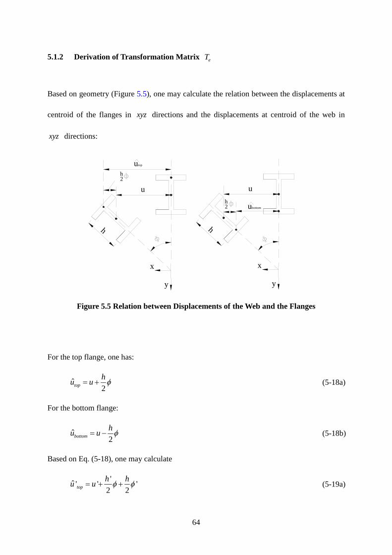
64
5.1.2 Derivation of Transformation Matrix eT
Based on geometry (Figure 5.5), one may calculate the relation between the displacements at
centroid of the flanges in xyz directions and the displacements at centroid of the web in
xyz directions:
u
utop
h2
h
y
x
u
ubottom
h
y
x
h2
Figure 5.5 Relation between Displacements of the Web and the Flanges
For the top flange, one has:
ˆ
2tophu u φ= + (5-18a)
For the bottom flange:
ˆ
2bottomhu u φ= − (5-18b)
Based on Eq. (5-18), one may calculate
'ˆ ' ' '2 2toph hu u φ φ= + + (5-19a)

65
'ˆ ' ' '2 2bottomh hu u φ φ= − − (5-19b)
where 0' 2 tanh α= .
Eqs. (5-18) and (5-19) may be implemented for node i to derive a transformation
matrix relating displacements of the centroid of the flanges in xyz directions to the
displacements of the centroid of the web in xyz directions:
For the top flange:
' '
''
1 0 0ˆ 2ˆ
0 1 tanˆ 20 0 1 0ˆ0 0 0 1
ii i
i iio
i i
ii Top
hu uu uhαφ φ
φφ
=
(5-20a)
For the bottom flange:
' '
''
1 0 0ˆ 2ˆ
0 1 tanˆ 20 0 1 0ˆ0 0 0 1
ii i
i iio
i i
ii Bottom
hu uu uhαφ φ
φφ
− − −=
(5-20b)
One may expand the matrices, Eq.(5-20), to an element including both nodes i and
j , the transformation matrix eT for both the top and bottom flanges are obtained.
66
For the top flange:
0
0
1 0 0 0 0 0 02
0 1 tan 0 0 0 02
0 0 1 0 0 0 0 00 0 0 1 0 0 0 0
( )0 0 0 0 1 0 0
2
0 0 0 0 0 1 tan2
0 0 0 0 0 0 1 00 0 0 0 0 0 0 1
i
i
e topj
j
h
h
T h
h
α
α
=
(5-21a)
For the bottom flange:
0
0
1 0 0 0 0 0 02
0 1 tan 0 0 0 02
0 0 1 0 0 0 0 00 0 0 1 0 0 0 0
( )0 0 0 0 1 0 0
2
0 0 0 0 0 1 tan2
0 0 0 0 0 0 1 00 0 0 0 0 0 0 1
i
i
e bottomj
j
h
h
T h
h
α
α
− − −
= − − −
(5-21b)
Finally, using Eqs. (5-17) and (5-21), one may express the displacements of the
centroid of the flanges as
ˆ[ ] [ ]e top e top etopflange webd T T d= (5-22a)
ˆ[ ] [ ]e bottom e bottom ebottomflange webd T T d= (5-22b)
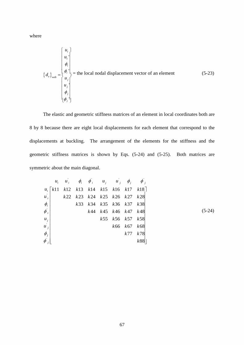
67
where
'
'
'
'
i
i
i
ie web
j
j
j
j
uu
duu
φφ
φφ
=
= the local nodal displacement vector of an element (5-23)
The elastic and geometric stiffness matrices of an element in local coordinates both are
8 by 8 because there are eight local displacements for each element that correspond to the
displacements at buckling. The arrangement of the elements for the stiffness and the
geometric stiffness matrices is shown by Eqs. (5-24) and (5-25). Both matrices are
symmetric about the main diagonal.
' ' ' '
'
'
'
'
11 12 13 14 15 16 17 1822 23 24 25 26 27 28
33 34 35 36 37 3844 45 46 47 48
55 56 57 5866 67 68
77 7888
i i i i j j j j
i
i
i
i
j
j
j
j
u u u u
u k k k k k k k ku k k k k k k k
k k k k k kk k k k k
u k k k ku k k k
k kk
φ φ φ φ
φφ
φφ
(5-24)
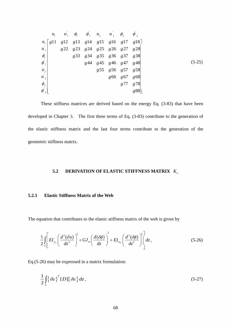
68
' ' ' '
'
'
'
'
11 12 13 14 15 16 17 1822 23 24 25 26 27 28
33 34 35 36 37 3844 45 46 47 48
55 56 57 5866 67 68
77 7888
i i i i j j j j
i
i
i
i
j
j
j
j
u u u u
u g g g g g g g gu g g g g g g g
g g g g g gg g g g g
u g g g gu g g g
g gg
φ φ φ φ
φφ
φφ
(5-25)
These stiffness matrices are derived based on the energy Eq. (3-83) that have been
developed in Chapter 3. The first three terms of Eq. (3-83) contribute to the generation of
the elastic stiffness matrix and the last four terms contribute to the generation of the
geometric stiffness matrix.
5.2 DERIVATION OF ELASTIC STIFFNESS MATRIX eK
5.2.1 Elastic Stiffness Matrix of the Web
The equation that contributes to the elastic stiffness matrix of the web is given by
22 22 2
2 2
1 ( ) ( ) ( )2 w wy w
L
d u d dEI GJ EI dzdz dz dzωδ δφ δφ + +
∫ , (5-26)
Eq.(5-26) may be expressed in a matrix formulation:
1 [ ]
2T
L
D dzδε δε∫ , (5-27)
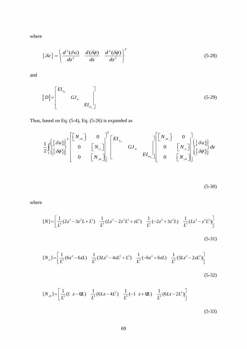
69
where
2 2
2 2
( ) ( ) ( )T
d u d ddz dz dzδ δφ δφδε
=
(5-28)
and
[ ]w
w
y
w
EI
D GJEIω
=
(5-29)
Thus, based on Eq. (5-4), Eq. (5-26) is expanded as
, ,
, ,
, ,
0 01 0 02
0 0
w
w
T
zz zzT y
z w zL
zz zz
N NEIu u
N GJ N dzEIN Nω
δ δ
δφ δφ
∫
(5-30)
where
3 2 3 3 2 2 3 3 2 3 2 2
3 3 3 3
1 1 1 1[ ] (2 3 ) ( 2 ) ( 2 3 ) ( )N z z L L Lz z L zL z z L Lz z LL L L L = − + − + − + −
(5-31)
2 2 2 3 2 2 2
, 3 3 3 3
1 1 1 1[ ] (6 6 ) (3 4 ) ( 6 6 ) (3 2 )zN z zL Lz zL L z zL Lz zLL L L L = − − + − + −
(5-32)
2 2
, 3 3 3 3
1 1 1 1[ ] (1 26 ) (6 4 ) ( 1 26 ) (6 2 )zzN z L Lz L z L Lz LL L L L = − − − + −
(5-33)
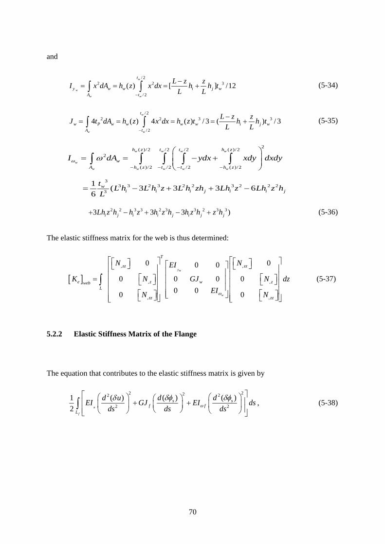
70
and
/ 22 2 3
/ 2
( ) [ ] /12w
w
w w
t
y w w i j wA t
L z zI x dA h z x dx h h tL L−
−= = = +∫ ∫ (5-34)
/ 22 2 3 3
/ 2
4 ( ) 4 ( ) / 3 ( ) / 3w
w w
t
w P w w w w i j wA t
L z zJ t dA h z x dx h z t h h tL L−
−= = = = +∫ ∫ (5-35)
2( )/2 /2 /2 ( )/22
( )/2 /2 /2 ( )/2
w w w w
w
w w w w w
h z t t h z
wA h z t t h z
I dA ydx xdy dxdyω ω− − − −
= = − +
∫ ∫ ∫ ∫ ∫
33 3 2 3 2 2 3 2 2 2
3
1 ( 3 3 3 66
wi i i j i i j
t L h L h z L h zh Lh z Lh z hL
= − + + −
2 2 3 3 2 3 3 2 3 33 3 3 )i j i i j i j jLh z h h z h z h h z h z h+ − + − + (5-36)
The elastic stiffness matrix for the web is thus determined:
[ ], ,
, ,
, ,
0 00 0
0 0 0 00 00 0
yw
w
T
zz zz
e z w zwebL
zz zz
N NEI
K N GJ N dzEIN Nω
=
∫ (5-37)
5.2.2 Elastic Stiffness Matrix of the Flange
The equation that contributes to the elastic stiffness matrix is given by
22 2 22
2 2
( ) ( )1 ( )2 n
f
s sf f
L
d dd uEI GJ EI dsds ds dsω
δφ δφδ + + ∫ , (5-38)
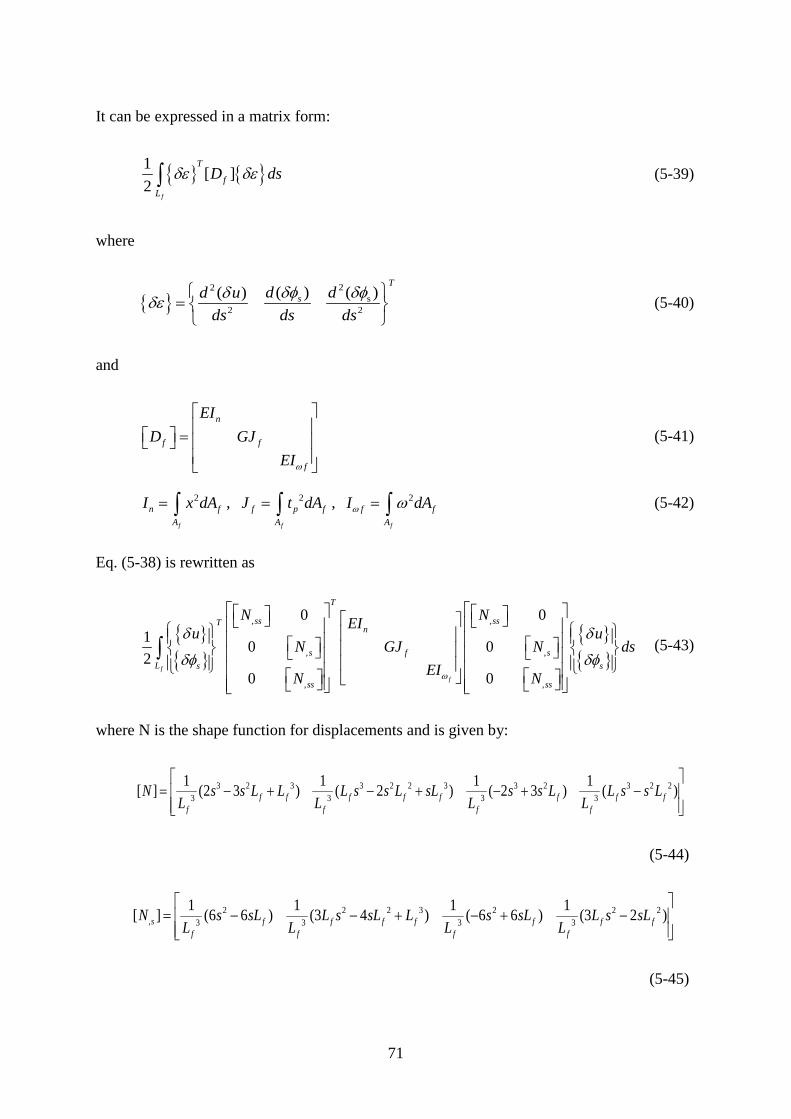
71
It can be expressed in a matrix form:
1 [ ]
2f
T
fL
D dsδε δε∫ (5-39)
where
22s
2 2
( ) ( )( )T
sd dd uds ds ds
δφ δφδδε
=
(5-40)
and
n
f f
f
EID GJ
EIω
=
(5-41)
2
f
n fA
I x dA= ∫ , 2
f
f p fA
J t dA= ∫ , 2
f
f fA
I dAω ω= ∫ (5-42)
Eq. (5-38) is rewritten as
, ,
, ,
, ,
0 01 0 02
0 0f
f
T
ss ssTn
s f sL s s
ss ss
N NEIu uN GJ N ds
EIN Nω
δ δ
δφ δφ
∫ (5-43)
where N is the shape function for displacements and is given by:
3 2 3 3 2 2 3 3 2 3 2 23 3 3 3
1 1 1 1[ ] (2 3 ) ( 2 ) ( 2 3 ) ( )f f f f f f f ff f f f
N s s L L L s s L sL s s L L s s LL L L L
= − + − + − + −
(5-44)
2 2 2 3 2 2 2, 3 3 3 3
1 1 1 1[ ] (6 6 ) (3 4 ) ( 6 6 ) (3 2 )s f f f f f f ff f f f
N s sL L s sL L s sL L s sLL L L L
= − − + − + −
(5-45)
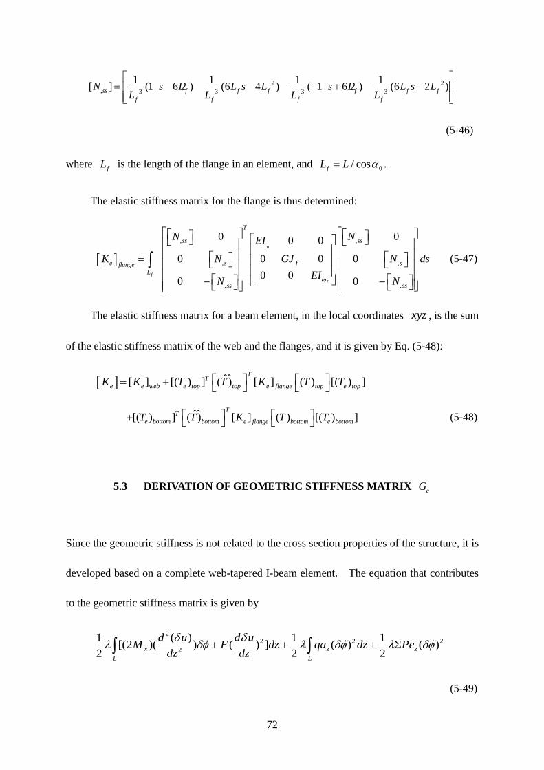
72
2 2, 3 3 3 3
1 1 1 1[ ] (1 26 ) (6 4 ) ( 1 26 ) (6 2 )ss f f f f f ff f f f
N s L L s L s L L s LL L L L
= − − − + −
(5-46)
where fL is the length of the flange in an element, and 0/ cosfL L α= .
The elastic stiffness matrix for the flange is thus determined:
[ ], ,
, ,
, ,
0 00 0
0 0 0 00 00 0
n
ff
T
ss ss
e s f sflangeL
ss ss
N NEI
K N GJ N dsEIN Nω
= − −
∫ (5-47)
The elastic stiffness matrix for a beam element, in the local coordinates xyz , is the sum
of the elastic stiffness matrix of the web and the flanges, and it is given by Eq. (5-48):
[ ] ˆˆ[ ] [( ) ] ( ) [ ] ( ) [( ) ]
TTe e web e top top e flange top e topK K T T K T T = +
ˆˆ[( ) ] ( ) [ ] ( ) [( ) ]
TTe bottom bottom e flange bottom e bottomT T K T T + (5-48)
5.3 DERIVATION OF GEOMETRIC STIFFNESS MATRIX eG
Since the geometric stiffness is not related to the cross section properties of the structure, it is
developed based on a complete web-tapered I-beam element. The equation that contributes
to the geometric stiffness matrix is given by
22 2 2
2
1 ( ) 1 1[(2 )( ) ( ) ] ( ) ( )2 2 2x z z
L L
d u d uM F dz qa dz Pedz dzδ δλ δφ λ δφ λ δφ+ + + Σ∫ ∫
(5-49)
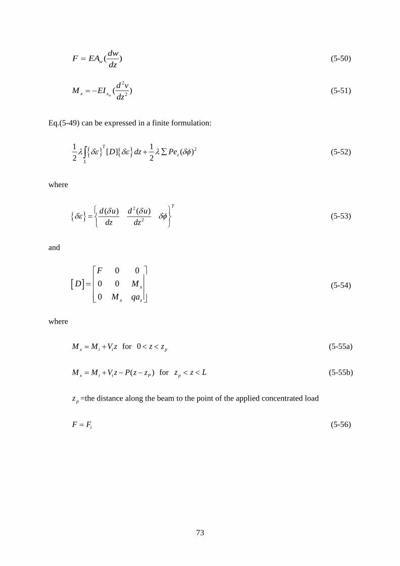
73
( )wdwF EAdz
= (5-50)
2
2( )wx x
d vM EIdz
= − (5-51)
Eq.(5-49) can be expressed in a finite formulation:
21 1[ ] ( )
2 2T
zL
D dz Peλ δε δε λ δφ+ ∑∫ (5-52)
where
2
2
( ) ( )T
d u d udz dzδ δδε δφ
=
(5-53)
and
[ ]0 0
0 00
x
x z
FD M
M qa
=
(5-54)
where
x i iM M V z= + for 0 pz z< < (5-55a)
( )x i i PM M V z P z z= + − − for pz z L< < (5-55b)
pz =the distance along the beam to the point of the applied concentrated load
iF F= (5-56)
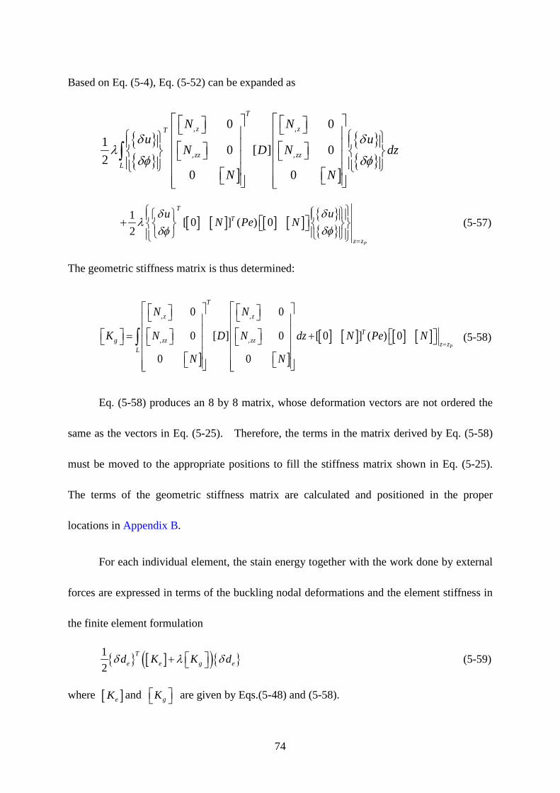
74
Based on Eq. (5-4), Eq. (5-52) can be expanded as
] ]
, ,
, ,
0 01 0 [ ] 02
0 0
T
z zT
zz zzL
N Nu u
N D N dz
N N
δ δλ
δφ δφ
∫
[ ] [ ] [ ] [ ]
1 [ 0 ] ( ) 02
P
TT
z z
uuN Pe N
δδλ
δφδφ=
+ (5-57)
The geometric stiffness matrix is thus determined:
] ]
[ ] [ ] [ ] [ ], ,
, ,
0 0
0 [ ] 0 [ 0 ] ( ) 0
0 0P
T
z z
Tg zz zz z z
L
N N
K N D N dz N Pe N
N N=
= +
∫ (5-58)
Eq. (5-58) produces an 8 by 8 matrix, whose deformation vectors are not ordered the
same as the vectors in Eq. (5-25). Therefore, the terms in the matrix derived by Eq. (5-58)
must be moved to the appropriate positions to fill the stiffness matrix shown in Eq. (5-25).
The terms of the geometric stiffness matrix are calculated and positioned in the proper
locations in Appendix B.
For each individual element, the stain energy together with the work done by external
forces are expressed in terms of the buckling nodal deformations and the element stiffness in
the finite element formulation
[ ]( ) 1
2T
e e g ed K K dδ λ δ + (5-59)
where [ ]eK and gK are given by Eqs.(5-48) and (5-58).
75
6.0 FLEXURAL-TORSIONAL BUCKLING EIGENVALUE
PROBLEM SOLUTION
A finite element analysis of the structured systems requires that the structure be divided into
several elements. The number and type of the elements depends on the geometry, material,
and loading condition of the structure. In this section, it is assumed that one is interested in
calculation of the flexural-torsional buckling load of a single tapered beam subjected to
arbitrary loading and stable support condition. Therefore, the beam is divided into n
elements. For each element, as it was shown in Chapter 5, the second variation of the total
potential energy in the global coordinate system may be expressed
[ ] [ ]( ) 21 1
2 2T
e e e e eD K G Dδ δ λ δ∏ = + (6-1)
Where
[ ]eK is the element elastic stiffness matrix in global coordinates
[ ]eG is the element geometric stiffness matrix in global coordinates
, ', , ', , ', , '
TTe i i i i j j j jD U U U Uδ δ δ δ δ δ δ δ δ= Φ Φ Φ Φ
(6-2)
To predict the buckling loads of the structure, the element matrices must be combined
together by the superposition process with respect to the degrees of freedom. Therefore, the
second variation of the total potential energy equation of the structure becomes:
76
[ ] [ ]( ) 0T
e eD K G Dδ λ δ∑ + ∑ = (6-3)
where
[ ]eK∑ is the structure global elastic stiffness matrix
[ ]eG∑ is the structure global geometric stiffness matrix
Since the variation of the displacement does not equal zero, Eq. (6-3) becomes
[ ] [ ]( ) 0e eK G Dλ δ∑ + ∑ = (6-4)
Eq. (6-4) is in the form of a generalized linear eigenvalue problem, and it can be
solved to determine the flexural-torsional buckling loads. A symmetric positive definite
matrix of order n has n eigenvalues λn and n non-zero eigenvectors δDn. The lowest
eigenvalue defines the load set at which the structure first buckles, and the corresponding
eigenvector defines the buckling mode of the structure.
In order to calculate the eigenvalues and eigenvectors of a generalized eigenvalue
problem, the problem should be converted to a standard eigenvalue problem (Griffiths and
Smith 1991). In other words, a generalized eigenvalue problem of the form
[ ] [ ]( ) 0A B Xλ+ = (6-5)
should be converted to the standard form of
[ ] [ ]( ) 0A I Xλ+ = (6-6)
where
[ ]I is the identity matrix.
To do so, one should first apply the Cholesky decomposition (Griffiths and Smith
1991) to the stiffness matrix [ ]K . The Cholesky decomposition is the numerical method to
77
decompose a square and symmetric matrix to the product of an upper triangular and the
transpose of the upper triangular matrix. This process can be written as
[ ] [ ][ ]TK C C= (6-7)
The next step is to substitute for the stiffness matrix in the generalized eigenvalue equation
(6-3) using Eq. (6-7)
( ) [ ][ ] [ ]TC C D G Dδ λ δ⋅ = − ⋅ (6-8)
Using premultiplication in Eq. (6-8), one may have
1[ ] [ ] [ ]TC D C G Dδ λ δ−⋅ = − ⋅ (6-9)
Introduce
[ ]TD C Dδ δ= ⋅ , or ( ) 1[ ]TD C Dδ δ
−= (6-10)
Substitute Eq. (6-10) in Eq. (6-9), one may have
( )( ) 11[ ] [ ] [ ]TD C G C Dδ λ δ
−−= − ⋅ (6-11)
Moving all the terms on the right side in Eq. (6-11) to the left, one may rewrite Eq. (6-12)
( )
11 1[ ] [ ] [ ] [ ] 0TC G C I Dδλ
−− + ⋅ =
(6-12)
Eq. (6-12) is in the form of a standard eigenvalue problem. It can be expressed more closely
to Eq. (6-5) if it is rewritten as
[ ] [ ]( ) 0S I Dγ+ = (6-13)
where
[ ] ( ) 11[ ] [ ] [ ]TS C G C−−=
(6-14)
1γλ
= (6-15)
78
The last step is to solve the standard eigenvalue problem. There are many numerical
methods to solve a standard eigenvalue problem, the selection of the methods depends on the
size of the matrix. Since the matrices in a flexural-torsional buckling problem can become
very large, the matrices may be converted to a simpler form using Householder’s method
before solving for the eigenvalues (Griffiths and Smith 1991). Householder’s method
converts a symmetric matrix into a tridiagonal matrix, a tridiagonal matrix has non-zero
elements only on the diagonal plus or minus one column (Press 1992). The eigenvalues of a
tridiagonal matrix may be then solved using QL iteration (Press 1992). The buckling loads
are the trial applied loads multiplied by the smallest eigenvalue, λ, which may be described
by the relationship
crF Fλ= (6-16)
where crF is the vector of the buckling loads, F is the vector of the trial loads, and λ
is a buckling parameter.
79
7.0 SOFTWARE DEVELOPMENT
There are many software packages that can be used to solve eigenvalues and eigenvectors of
a standard eigenvalue problem. However, the solution of a generalized eigenvalue problem
in our research is a complex and time consuming process for large matrices. Therefore, our
aim is to develop a software package of special purpose to determine the flexural-torsional
buckling load of a doubly-symmetric web-tapered I-beam.
Object-oriented technology can be defined as a method of analysis, design and
implementation of software that considers a problem as a real world situation. This
technology was selected for the program design and implementation over other software
development technologies because of the numerous advantages it offers in software
organization and that it can support a finite element application. Unlike traditional
procedural programming languages, object-oriented programming languages focus on
breaking the software into modular units, and each unit is modeled based upon a real-world
concept, not a computer concept. Since the models are close to a real problem, a more
precise and concise software can be developed. This programming approach was developed
to provide a more organized methodology to software development in comparison to the
older disorganized approaches.
80
There are many languages that support object-oriented design, including Smalltalk,
Eiffel, C++, and etc. There is no particular object-oriented language superior to the others;
rather, it is best to select a programming language based on its ability to provide sufficient
support of the desired programming style (Stroustrup 1991). The object-oriented language
used in this program design is C/C++.
C/C++ is a structured language convenient for software development or revision, and
it is also a mid-level language that can be used as a high-level language, and can directly
access the hardware like a low-level language. Among many programming languages,
C/C++ was selected because it has become one of the most popular ones that support
object-oriented design.
7.1 OBJECT-ORIENTED MODELING AND PROGRAMMING CONCEPTS
The fundamental idea behind object-oriented languages is to combine into a single unit both
data and the functions that operate on that data. Such a unit is called an object; it is the
smallest unit of a system. This concept of combining data and functions into one entity is
known as encapsulation. An object’s functions, called member functions in C++, typically
provide a secure way to access the data. An object may call on another object’s member
functions in order to perform an operation or to retrieve some data. However, objects have
the ability to limit the access of their data and member functions from other objects so that
the information cannot be accessed directly. The data is hidden, so it is safe from accidental
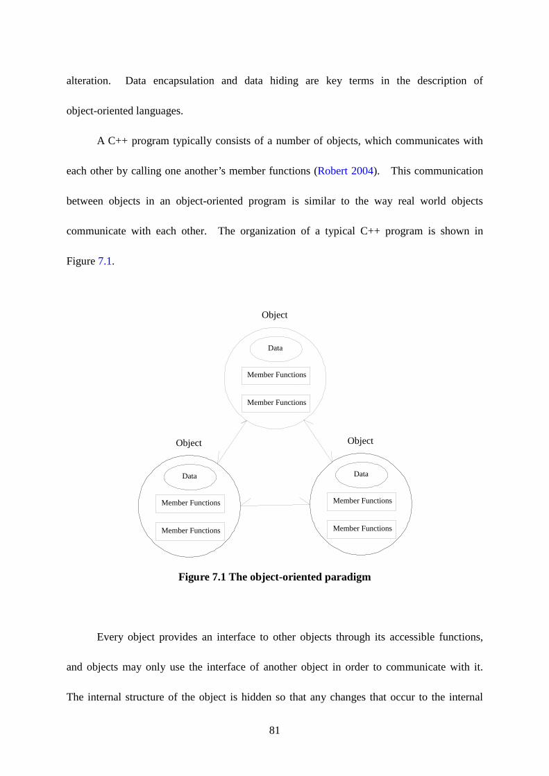
81
alteration. Data encapsulation and data hiding are key terms in the description of
object-oriented languages.
A C++ program typically consists of a number of objects, which communicates with
each other by calling one another’s member functions (Robert 2004). This communication
between objects in an object-oriented program is similar to the way real world objects
communicate with each other. The organization of a typical C++ program is shown in
Figure 7.1.
Member Functions
Member Functions
Data
Object
Member Functions
Member Functions
Data
Object
Member Functions
Member Functions
Data
Object
Figure 7.1 The object-oriented paradigm
Every object provides an interface to other objects through its accessible functions,
and objects may only use the interface of another object in order to communicate with it.
The internal structure of the object is hidden so that any changes that occur to the internal
82
structure will only affect the object’s implementation. When an instance of either class is
created, other objects may only access the object properties that are declared public within
the code. Private and protected data and member functions have restricted access by other
objects. Therefore, the public features of a class make up the interface of an object of that
class, and the private and protected features of an object are used to aid in the object’s
implementation.
An object must have four characteristics (Rumbaugh et al. 1991): identity,
classification, polymorphism, and inheritance.
Each object has an identity. Even if all the properties of two different objects are
identical, their identities are not the same; each has a unique identifier or handle. Often,
object-oriented programming systems assign invisible arbitrary numbers to serve as handles.
A group of objects cannot combine into a new object, but they may form a class if they
share common properties, characteristics, or legal operations. A class is the outline, or
template, of an object; it describes all of the attributes and operations that an object of its type
contains, as shown by Figure 7.2 below. A class is only an abstraction, while an object
represents an actual real world item. Once a class is defined, many objects of that class may
be created with each object being unique yet possessing all of the same features as the other
objects. Each object is created at run-time according to the class specification and is said to
be an instance of a class.
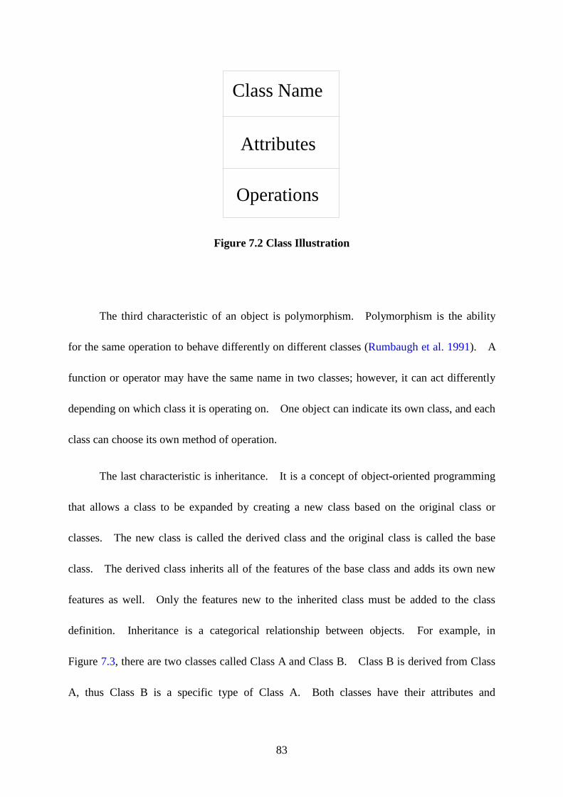
83
Class Name
Attributes
Operations
Figure 7.2 Class Illustration
The third characteristic of an object is polymorphism. Polymorphism is the ability
for the same operation to behave differently on different classes (Rumbaugh et al. 1991). A
function or operator may have the same name in two classes; however, it can act differently
depending on which class it is operating on. One object can indicate its own class, and each
class can choose its own method of operation.
The last characteristic is inheritance. It is a concept of object-oriented programming
that allows a class to be expanded by creating a new class based on the original class or
classes. The new class is called the derived class and the original class is called the base
class. The derived class inherits all of the features of the base class and adds its own new
features as well. Only the features new to the inherited class must be added to the class
definition. Inheritance is a categorical relationship between objects. For example, in
Figure 7.3, there are two classes called Class A and Class B. Class B is derived from Class
A, thus Class B is a specific type of Class A. Both classes have their attributes and
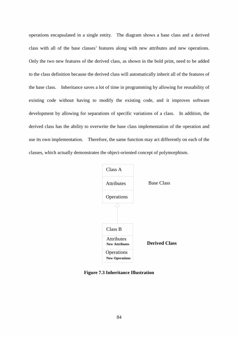
84
operations encapsulated in a single entity. The diagram shows a base class and a derived
class with all of the base classes’ features along with new attributes and new operations.
Only the two new features of the derived class, as shown in the bold print, need to be added
to the class definition because the derived class will automatically inherit all of the features of
the base class. Inheritance saves a lot of time in programming by allowing for reusability of
existing code without having to modify the existing code, and it improves software
development by allowing for separations of specific variations of a class. In addition, the
derived class has the ability to overwrite the base class implementation of the operation and
use its own implementation. Therefore, the same function may act differently on each of the
classes, which actually demonstrates the object-oriented concept of polymorphism.
Class A
Attributes
Operations
Class B
Attributes
Operations
New Attributes
New Operations
Base Class
Derived Class
Figure 7.3 Inheritance Illustration
85
Objects, classes, polymorphism, and inheritance are only a few of the many
object-oriented concepts. These are just the beginning to all of the advantages that
object-oriented programming has to offer. More specific concepts will be discussed
throughout the program development in the following sections. One technical advancement
that has brought object-oriented concepts to the point that they are at today is abstraction.
Abstraction allows a programmer to focus on the overall entity under consideration without
getting mired in the details. This means focusing on defining an object rather than on the
implementation of an object. When an object user needs information from the object, the
user needs to know what the object is and does, rather than how the object is implemented.
The goal of abstraction is “to isolate those aspects that are important for some purpose and
suppress those aspects that are unimportant” (Rumbaugh et al. 1991).
7.2 PROGRAM DESIGN
The development of the executable program required for this project necessitated a software
package designed by Phusit Dontree (1994). The LBuck program developed by Dontree
was written in C++; however, many of the features of the programming were outdated and
only applicable to uniform I-beams. The goal is to rework the original LBuck program to
make it applicable to doubly-symmetric web-tapered I-beams. In object-oriented
terminology, this process is known as refactoring.
86
The term refactoring is used to describe a technique of changing the internal structure
of a program in order to make it easier to understand and cheaper to modify, without
changing its observable behavior (Fowler 1999). The decision to refactor the existing
program rather than start from scratch owes to many features that work well in original
LBuck program. By refactoring the program, the design of the software can be improved
and utilized for any researcher’s purpose. Kent Beck (as quoted in Fowler, 1999), who was
one of the first people to recognize the importance of refactoring, stated four main things that
make a program hard to work with: 1) programs that are hard to read are hard to modify, 2)
programs that have duplicate logic are hard to modify, 3) programs that require additional
behavior that requires you to change running code are hard to modify, and 4) programs with
complex conditional logic are hard to modify. These four main issues will be seriously
considered while refactoring the program.
Object-oriented software development must follow a specific design process. This
process must outline every single step during the design of the program from the abstract
concepts to the detailed codes. The Rational Unified Process developed by Grady Booch,
James Rumbaugh, and Ivar Jacobson (Jacobson et al. 1999) provides a modern approach to
software development which can be tailored to model real world situations. This approach
consists of four main phases: inception, elaboration, construction, and transition, which is
shown in Figure 7.4.
The inception phase is where the scope of the project is determined. Also the core
architecture will be established, and the critical risk while assuring feasibility is identified and

87
reduced (Jacobson 2000). The elaboration phase is the stage where all of the details are
collected to create a plan for the construction. The construction phase is where the system is
built, which involves many iterations. The transition phase is the stage where any work left
until the end must be completed, such as specific forms of testing.
Inception
Elaboration
Construction
Transition
Iteration
Figure 7.4 Rational Unified Process
The design process is going to focus on the LBuck programs. And the details of each
phase will be discussed in the following sections.
88
7.3 OBJECT-ORIENTED MODELING AND PROGRAMMING
FLEXURAL-TORSIONAL BUCKLING PROBLEMS
This section explains the details of each phase of the software development of the
flexural-torsional buckling problem of doubly symmetric web-tapered I-beams: inception,
elaboration, construction and the transition.
7.3.1 Inception
For the inception phase of the project, the scope may be summarized as: refactor an existing
program that calculates the flexural-torsional buckling loads of a beam.
7.3.2 Elaboration
This phase begins with a technique called use case modeling. Use case modeling intends to
communicate with the user how the system and its environment are related, it is one of the
most important parts in software development. This process will ensure that the client and
other program developers of the design will understand the users’ needs. Use cases have
two important roles: (1) they capture a system’s functional requirements and (2) they
structure each object model into a manageable view (Jacobson 2000).
The first step in developing the use cases is to determine the actors. An actor is
something or someone that will use the system. Actors do not need to be human, and it can
89
be other systems that require information from the current system. For this particular
program, the actor is the Project program, which is the user interface. The user interface is
the system that calls on the LBuck to execute, and it requires the flexural-torsional buckling
loads of the structure from the program.
The next step is to consider all scenarios that need to deal with. A scenario is a
sequence of steps describing an interaction between an actor and a system (Fowler 2000). A
group of related scenarios is a use case. For this particular program, the scenario is the
flexural-torsional buckling analysis of a doubly symmetric web-tapered I-beam. The user
interaction for this scenario makes up the use case model, and it is essentially inputting
background information to calculate the flexural-torsional buckling loads of the structure.
It is important to provide detailed descriptions of the use case along with the diagram.
The description of the use case for the program is: the user enters into the program the
structure properties, dimensions, loads, and restraints. The program uses the data to
calculate the flexural-torsional buckling load of the structure.
In this stage, it is also necessary to understand the operations of the LBuck program,
and to collect all of the details needed for the refactoring process in the construction phase of
the program. Figure 7.5 shows the refactoring process of the construction phase (Robert
2004). The goal is to modify the original code and rebuild new models based on current
research needs.
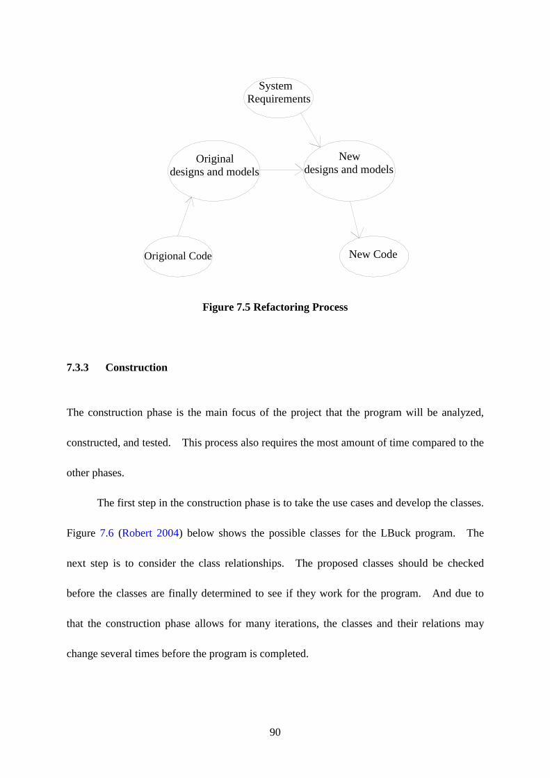
90
SystemRequirements
Originaldesigns and models
Origional Code
Newdesigns and models
New Code
Figure 7.5 Refactoring Process
7.3.3 Construction
The construction phase is the main focus of the project that the program will be analyzed,
constructed, and tested. This process also requires the most amount of time compared to the
other phases.
The first step in the construction phase is to take the use cases and develop the classes.
Figure 7.6 (Robert 2004) below shows the possible classes for the LBuck program. The
next step is to consider the class relationships. The proposed classes should be checked
before the classes are finally determined to see if they work for the program. And due to
that the construction phase allows for many iterations, the classes and their relations may
change several times before the program is completed.
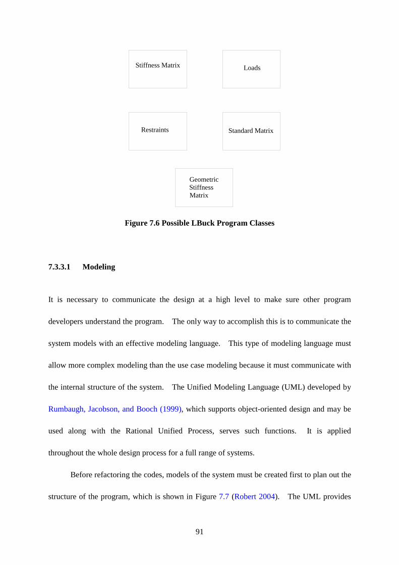
91
Stiffness Matrix Loads
Standard MatrixRestraints
GeometricStiffnessMatrix
Figure 7.6 Possible LBuck Program Classes
7.3.3.1 Modeling
It is necessary to communicate the design at a high level to make sure other program
developers understand the program. The only way to accomplish this is to communicate the
system models with an effective modeling language. This type of modeling language must
allow more complex modeling than the use case modeling because it must communicate with
the internal structure of the system. The Unified Modeling Language (UML) developed by
Rumbaugh, Jacobson, and Booch (1999), which supports object-oriented design and may be
used along with the Rational Unified Process, serves such functions. It is applied
throughout the whole design process for a full range of systems.
Before refactoring the codes, models of the system must be created first to plan out the
structure of the program, which is shown in Figure 7.7 (Robert 2004). The UML provides
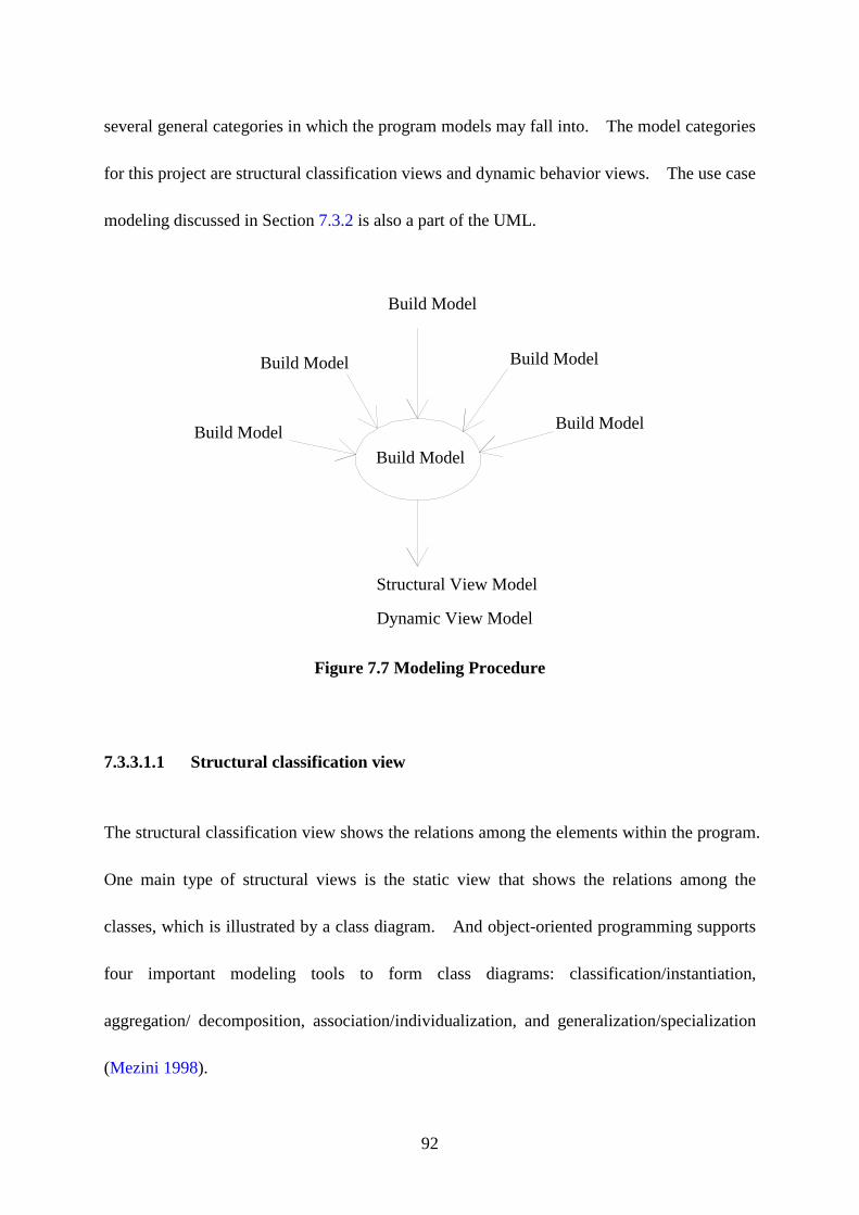
92
several general categories in which the program models may fall into. The model categories
for this project are structural classification views and dynamic behavior views. The use case
modeling discussed in Section 7.3.2 is also a part of the UML.
Build ModelBuild Model
Build Model
Build Model
Build Model
Build Model
Structural View Model
Dynamic View Model
Figure 7.7 Modeling Procedure
7.3.3.1.1 Structural classification view
The structural classification view shows the relations among the elements within the program.
One main type of structural views is the static view that shows the relations among the
classes, which is illustrated by a class diagram. And object-oriented programming supports
four important modeling tools to form class diagrams: classification/instantiation,
aggregation/ decomposition, association/individualization, and generalization/specialization
(Mezini 1998).
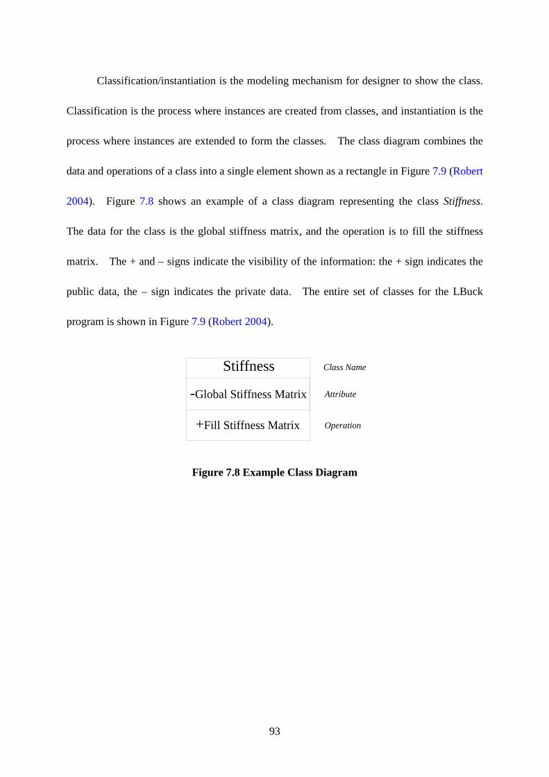
93
Classification/instantiation is the modeling mechanism for designer to show the class.
Classification is the process where instances are created from classes, and instantiation is the
process where instances are extended to form the classes. The class diagram combines the
data and operations of a class into a single element shown as a rectangle in Figure 7.9 (Robert
2004). Figure 7.8 shows an example of a class diagram representing the class Stiffness.
The data for the class is the global stiffness matrix, and the operation is to fill the stiffness
matrix. The + and – signs indicate the visibility of the information: the + sign indicates the
public data, the – sign indicates the private data. The entire set of classes for the LBuck
program is shown in Figure 7.9 (Robert 2004).
Stiffness
-Global Stiffness Matrix
+Fill Stiffness Matrix
Class Name
Attribute
Operation
Figure 7.8 Example Class Diagram
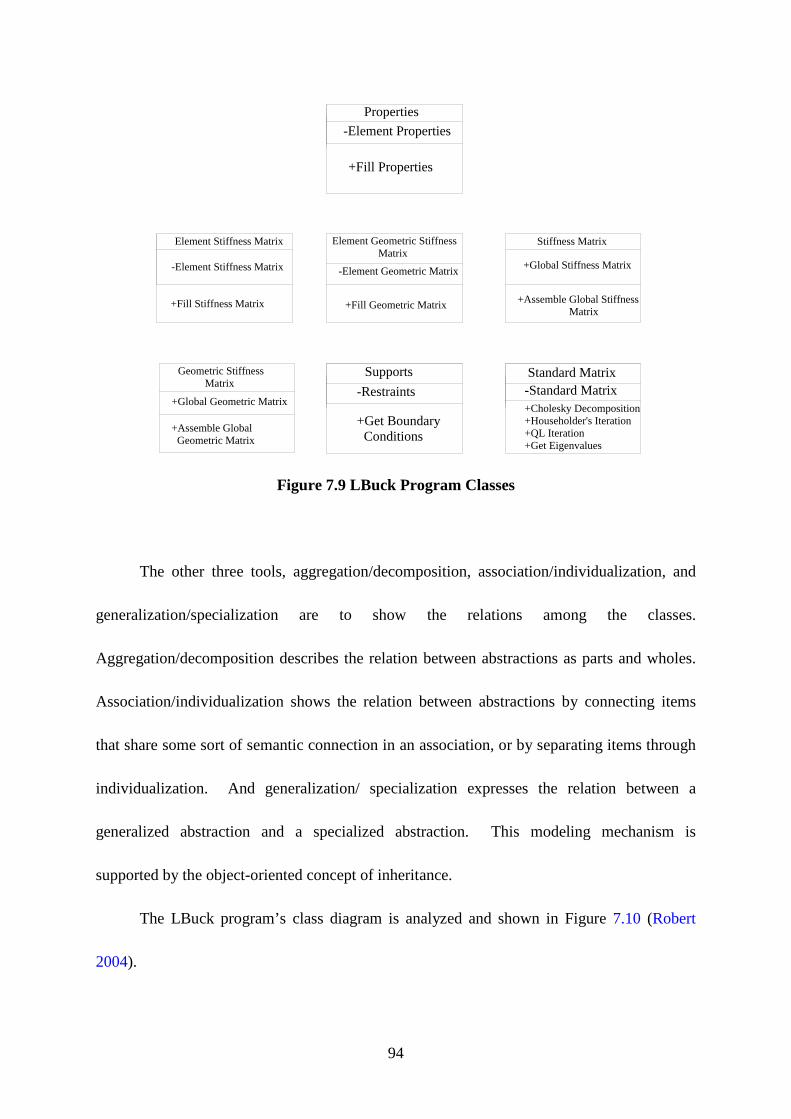
94
Properties-Element Properties
+Fill Properties
Element Stiffness Matrix
-Element Stiffness Matrix
+Fill Stiffness Matrix
Element Geometric Stiffness Matrix
-Element Geometric Matrix
+Fill Geometric Matrix
Stiffness Matrix
+Global Stiffness Matrix
+Assemble Global Stiffness Matrix
Supports-Restraints
+Get Boundary Conditions
Standard Matrix-Standard Matrix+Cholesky Decomposition+Householder's Iteration+QL Iteration+Get Eigenvalues
Geometric Stiffness Matrix
+Global Geometric Matrix
+Assemble Global Geometric Matrix
Figure 7.9 LBuck Program Classes
The other three tools, aggregation/decomposition, association/individualization, and
generalization/specialization are to show the relations among the classes.
Aggregation/decomposition describes the relation between abstractions as parts and wholes.
Association/individualization shows the relation between abstractions by connecting items
that share some sort of semantic connection in an association, or by separating items through
individualization. And generalization/ specialization expresses the relation between a
generalized abstraction and a specialized abstraction. This modeling mechanism is
supported by the object-oriented concept of inheritance.
The LBuck program’s class diagram is analyzed and shown in Figure 7.10 (Robert
2004).
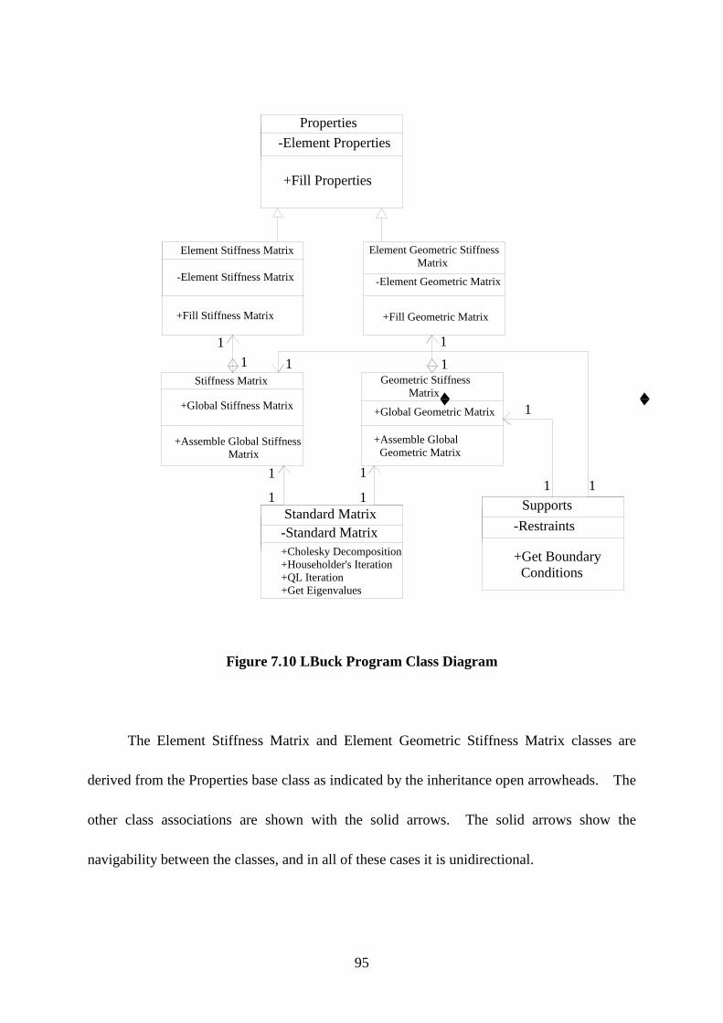
95
Properties-Element Properties
+Fill Properties
Element Stiffness Matrix
-Element Stiffness Matrix
+Fill Stiffness Matrix
Element Geometric Stiffness Matrix
-Element Geometric Matrix
+Fill Geometric Matrix
Stiffness Matrix
+Global Stiffness Matrix
+Assemble Global Stiffness Matrix
Supports-Restraints
+Get Boundary Conditions
Standard Matrix-Standard Matrix+Cholesky Decomposition+Householder's Iteration+QL Iteration+Get Eigenvalues
Geometric Stiffness Matrix
+Global Geometric Matrix
+Assemble Global Geometric Matrix
1
1 1
1111 1
1
1
1
1
Figure 7.10 LBuck Program Class Diagram
The Element Stiffness Matrix and Element Geometric Stiffness Matrix classes are
derived from the Properties base class as indicated by the inheritance open arrowheads. The
other class associations are shown with the solid arrows. The solid arrows show the
navigability between the classes, and in all of these cases it is unidirectional.
96
One of the new features shown on the diagram is the black diamond which is used to
indicate composition. Composition is another one of the basic concepts of object-oriented
programming. Composition is a specific form of aggregation. This shows the conceptual
relationship of an element stiffness matrix being a part of a global stiffness matrix.
Composition is a stronger form of aggregation where the part may belong to only one whole
and the life of the part is the life of the whole. The Stiffness Matrix and the Geometric
Stiffness Matrix classes are the “whole” and the Element Stiffness Matrix and Element
Geometric Stiffness Matrix classes are the “parts”. The Standard Matrix class must be
associated with the Stiffness Matrix and the Geometric Stiffness Matrix classes in order to
calculate the standard matrix. The Restraints are applied to both the stiffness matrix and the
geometric stiffness matrix; therefore, associations between these classes are indicated. At
the ends of the arrows are numbers indicating the multiplicity of the instances of the classes
with (*) denoting infinity. For example, a Stiffness matrix object may be associated with
anywhere from one to an infinite number of element stiffness matrices at a conceptual level;
however, each element stiffness matrix may be associated with only one stiffness matrix.
The ordered keyword is a constraint implying there is an ordering of the objects that it is
associated with and that a particular object can appear on the total list of objects only once.
7.3.3.1.2 Dynamic behavior view
The dynamic behavior view provides a visual model of the system over a period of time, and
it helps developers to understand which objects are instantiated and how the objects interact
97
with each other during the program execution. A sequence diagram is a specific type of
dynamic behavior view that displays the interaction as a two-dimensional chart. The
sequence diagram of LBuck program is shown in Figure 7.11 (Robert 2004). It is important
to notice that all of the same behaviors are being implemented in this model, only now the
behaviors are redistributed among the objects to enhance the object-oriented features of the
program design.
The assemble Stiffness process creates a new element stiffness matrix object for each
element in the discretized structure. Each element object reads the properties for the
element and fills the matrix in the Fill_Element_Matrix process. Each matrix is sent back to
the Stiffness Matrix object and assembled into the appropriate position in the global stiffness
matrix. The exact same process occurs for the Geometric Matrix object. The assemble
Geometric process creates a new Element Geometric Matrix object for each element in the
discretized structure. Each element object reads the properties for the element and fills the
element geometric stiffness matrix in the Fill_Element_Matrix process. Each element
matrix is sent back to the Geometric Matrix object and assembled into the appropriate
position in the global stiffness matrix.
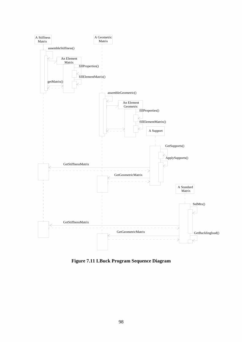
98
A Stiffness Matrix
A Geometric Matrix
assembleStiffness()
An Element Matrix
fillProperties()
fillElementMatrix()
assembleGeometric()
An Element Geometric
fillProperties()
fillElementMatrix()
A Support
GetSupports()
ApplySupports()
GetGeometricMatrix
GetStiffnessMatrix
GetStiffnessMatrix
GetGeometricMatrix
A Standard Matrix
StdMtx()
GetBucklingload()
getMatrix()
Figure 7.11 LBuck Program Sequence Diagram
99
The support object reads in the supports in the getSupports process. It applies the
boundary conditions to the structure in the applySupports process. The Standard Matrix
object changes the generalized eigenvalue problem to the standard eigenvalue problem.
Consequently, the global stiffness matrix and global geometric stiffness matrix are combined
to the standard matrix. The standard matrix is then solved for the eigenvalues. The final
step is the print process. This process is different depending on the type of analysis. For
the buckling analysis, the buckling parameter, or eigenvalue, is printed as the result of the
anlaysis. The buckling load is the multiplication of the eigenvalue and the trial loads. For
the prebuckling anlaysis, the eigenvalue is checked within the print process before the results
are printed. If the eigenvalue is not equal to one, the eigenvalue is returned to the beginning
of the program as a multiplication factor. The trial loads are multiplied by the multiplication
factor and the entire process starts again. The program continues until the eigenvalue is
close to one, and the trial loads for that iteration are the buckling loads.
It is often difficult to understand the flow of behaviors within a program, and dynamic
behavior views help to model the flow control so that the sequence of behaviors become
apparent. The sequence diagrams for both the Frame and LBuck programs help to increase
the clarity of how the objects collaborate within the program during its implementation.
An activity diagram is another type of dynamic behavior view. “An activity graph
shows the computational activities involved in performing a calculation” (Rumbaugh et al.
1991). It describes a sequence of activities and helps when trying to understand the flow
of work in a calculation. Activity diagrams are much like flowcharts except that they allow
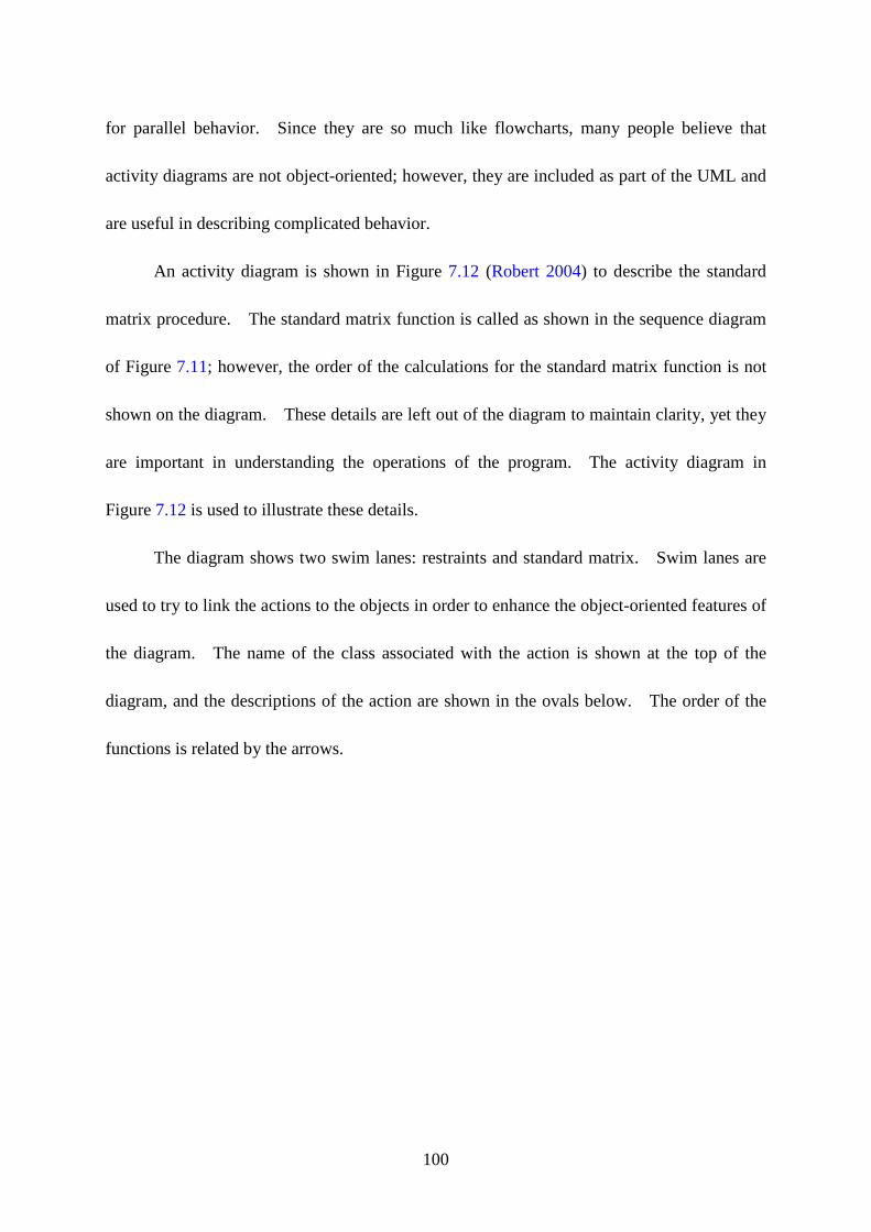
100
for parallel behavior. Since they are so much like flowcharts, many people believe that
activity diagrams are not object-oriented; however, they are included as part of the UML and
are useful in describing complicated behavior.
An activity diagram is shown in Figure 7.12 (Robert 2004) to describe the standard
matrix procedure. The standard matrix function is called as shown in the sequence diagram
of Figure 7.11; however, the order of the calculations for the standard matrix function is not
shown on the diagram. These details are left out of the diagram to maintain clarity, yet they
are important in understanding the operations of the program. The activity diagram in
Figure 7.12 is used to illustrate these details.
The diagram shows two swim lanes: restraints and standard matrix. Swim lanes are
used to try to link the actions to the objects in order to enhance the object-oriented features of
the diagram. The name of the class associated with the action is shown at the top of the
diagram, and the descriptions of the action are shown in the ovals below. The order of the
functions is related by the arrows.
101
Restraints Standard Matrix
ReceiveStiffnessMatricesK and G
ApplyBoundaryConditions
ApplyCholeskyMethod
ApplyHouseholder'sIteration
ApplyQLIteration
CheckEigenValues
Figure 7.12 Activity Diagram
7.3.3.2 Coding
Once the abstract models are completed, the design can move back to the coding process.
Two-dimensional arrays are used in the classes to store the matrices. Passing an array as an
102
argument between two functions is different from passing other types of variables. The
name of an array is its address, and arrays must be passed by their names, or addresses.
Normally, there are two ways for an object to access the array of another object: (1) make the
array public data, (2) make the two objects friends to each other.
The coding for LBuck program begins with defining the classes:
class Properties
protected:
int j1,j2,joint_num;
float E,G,Jf,Iwf,L,Lf,In,tw,d,zi,zj,hi,hj,tanA0,A0,element_num,length;
float Fi,Vi,Vj,Mi;
float z[MSize];
float h[MSize];
float v[MSize];
float mi[MSize];
public:
virtual void Fill_Properties(int, int, float)=0;
;
The Properties class stores the properties of the structure. The Fill_Properties ()
function stores the properties in matrix form.
103
class Element_Stiffness:public Properties
private:
float KE[MSize][MSize];
float EW[MSize][MSize];
float EF[MSize][MSize];
float P[MSize][MSize];
float Q[MSize][MSize];
float PT[MSize][MSize];
float QT[MSize][MSize];
float C[MSize][MSize];
float CT[MSize][MSize];
float DT[MSize][MSize];
float D[MSize][MSize];
float X1[MSize][MSize];
float X2[MSize][MSize];
float X3[MSize][MSize];
float X4[MSize][MSize];
float Y1[MSize][MSize];
float Y2[MSize][MSize];
float Y3[MSize][MSize];
104
float Y4[MSize][MSize];
public:
friend int main();
friend class Stiffness;
void Fill_Element_Stiffness(float, int, float);
void Fill_Properties(int, int, float);
;
The Element_Stiffness class is derived from the Properties class. The
Fill_Element_Stiffness1 () function fills the buckling stiffness matrix. And the stiffness
matrix will be stored in the KE two-dimensional array.
class Element_Geometric:public Properties
private:
float KG[MSize][MSize];
float GW[MSize][MSize];
float GF[MSize][MSize];
float P[MSize][MSize];
float Q[MSize][MSize];
float PT[MSize][MSize];
float QT[MSize][MSize];
float C[MSize][MSize];
105
float CT[MSize][MSize];
float DT[MSize][MSize];
float D[MSize][MSize];
float X1[MSize][MSize];
float X2[MSize][MSize];
float X3[MSize][MSize];
float X4[MSize][MSize];
float Y1[MSize][MSize];
float Y2[MSize][MSize];
float Y3[MSize][MSize];
float Y4[MSize][MSize];
public:
friend class Geometric;
void Fill_Element_Geometric(float,int,float);
void Fill_Properties(int, int, float);
;
The Element_Geometric class is also derived from the Properties class. The
Fill_Element_Geometric () function fills the buckling geometric stiffness matrix. The
geometric stiffness matrix is stored in the GE two a dimensional array.
106
class Stiffness
private:
Element_Stiffness stiff; //Element Stiffness matrix
int element_num;//number of elements
float length;
public:
float A[MSize][MSize];
Stiffness(int);
void Assembling_Stiffness_Matrix(float,int,float);
;
The Stiffness class contains an Element_Stiffness matrix object. Each element
stiffness matrix will be assembled into the global stiffness matrix, A, using the
Assembling_Stiffness_Matrix () function, and then deleted in order to save memory space.
class Geometric
private:
Element_Geometric geom; //element geometric matrix
int element_num; //number of elements
float length;
public:
107
float B[MSize][MSize];
Geometric(int);
void Assembling_Geometric_Matrix(float,int,float);
;
Similarly, there is an Element_Geometric matrix object. And each element
geometric stiffness matrix will be assembled into global geometric stiffness matrix, B, using
the Assembling_Stiffness_Matrix () function.
class Standard_Matrix
private:
int size;
float dia[MSize];
float C[MSize][MSize];
float off[MSize];
float buckling_load;
public:
Standard_Matrix();
void standard_matrix(float[MSize][MSize],float[MSize][MSize],int);
float pythag(float,float);
void choldc(float[MSize][MSize]);
void tred2(float[MSize][MSize]);
108
void tqli(float[MSize][MSize]);
float getBucklingLoad();
;
The Standard_Matrix class creates the standard eigen-value problem from the elastic
stiffness matrix and the geometric stiffness matrix. The Standard_Matrix () function calls
upon the functions choldc (), tred2 (), and tqli (), in addition, it is the function used to store
the standard matrix. The pythag () function is the Pythagorean function. The choldc ()
function is the Cholesky method which changes the stiffness matrix to the upper triangular
matrix (Press 1992). The tred2 () function displays the Householder’s iteration which
changes the standard matrix to a tridiagonal matrix. And the eigenvlaue of the tridiagonal
matrix will be calculated in tqli () function through QL iteration (Press 1992).
class Supports
private:
int restrain[MSize];
int rest;
int size; //Total degrees of freedom
int free_size; //Free degrees of freedom
public:
Supports(int);
void Get_boundary_conditions();
109
int Boundary_Condition(float[MSize][MSize],float[MSize][MSize]);
;
The Supports class is used to store the restraint information. The
Get_boundary_conditions () function is used to input the boundary conditions. The
Boundary_Condition () function is used to apply the restraints to the global stiffness and
geometric stiffness matrices.
The source files now should be implemented to the classes. The original program
provided the data that are only applicable to doubly symmetric uniform I-beams, therefore,
those codes have to be modified and reorganized.
7.3.4 Transition
The transition phase is the last stage in the design process, which focuses on testing and
fixing bugs. The goal of this phase is to ensure that the product is applicable to practical use.
In this stage, the testing will be conducted to compare the results of the program with those of
the existing solutions. Once the transition phase is completed, the program is ready to use.
The complete program code for the LBuck programs is in Appendix C.
110
8.0 FLEXURAL-TORSIONAL BUCKLING OF BEAMS: EXAMPLES
The buckling load is an important criterion for the structural steel design. In this chapter,
three example cases, the cantilever with a tip concentrated load, the beam subjected to free
end moments with different boundaries, and the simply supported tapered beam with two
equal end moments, are analyzed using the LBUCK program developed in this research.
The second variation of the total potential energy presented in Chapter 3, in which the
prebuckling behavior is disregarded, is used in conjunction with finite element methods to
develop the computer program. The LBUCK program will be verified by comparing the
lateral buckling loads of beams with results from typical theories in existing literatures.
8.1 BUCKLING ANALYSIS: EXAMPLE 1
Since the lateral buckling loads of prismatic uniform thin-walled beams have been
extensively investigated and widely accepted, a cantilever of uniform I-section is analyzed to
help verify the program developed in this paper.
A cantilevered beam with a concentrated load at the free end is analyzed first (See
Figure 8.1). The load is applied at the shear center. The properties of the cantilever are E
= 210 GPa (30458 ksi), ν = 0.3, h = 600 mm (23.62 in), ft = 10 mm (0.394 in), wt = 8 mm
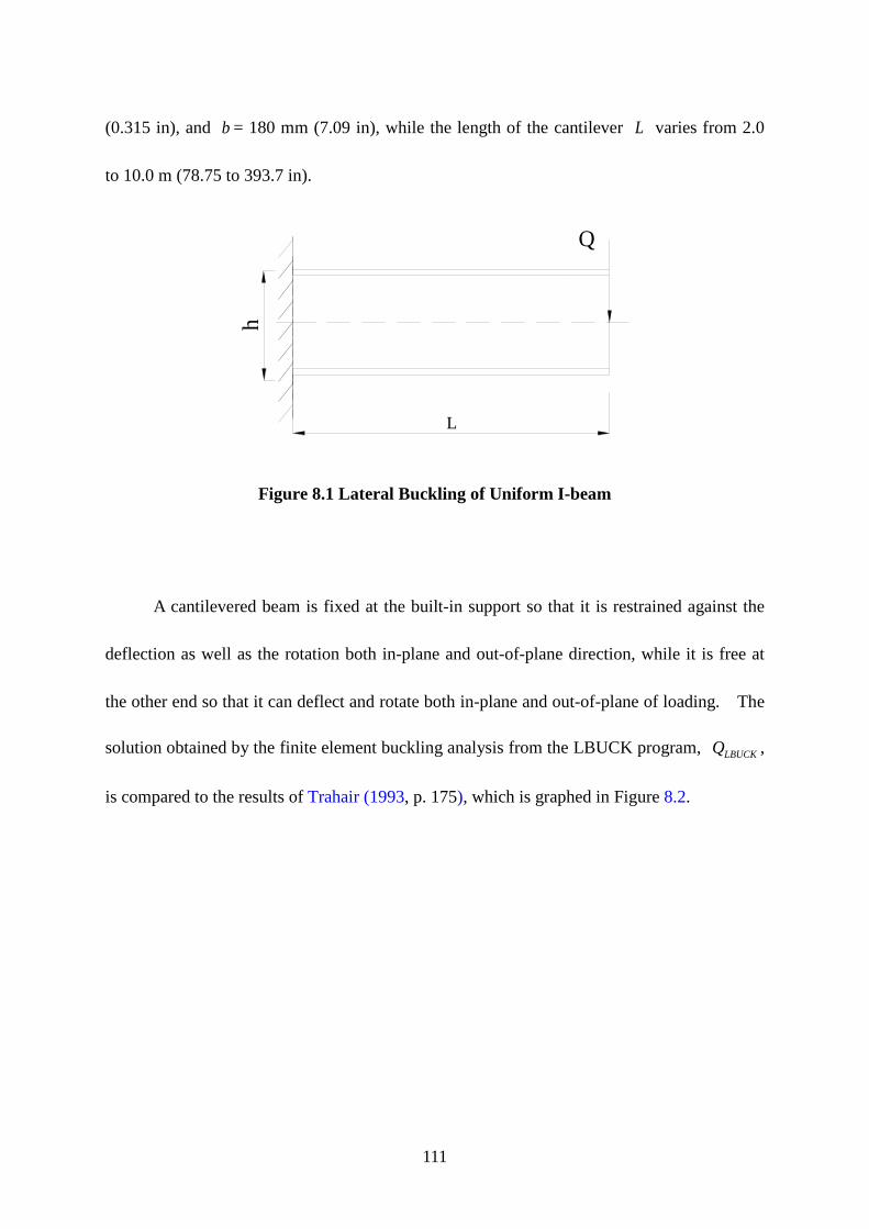
111
(0.315 in), and b = 180 mm (7.09 in), while the length of the cantilever L varies from 2.0
to 10.0 m (78.75 to 393.7 in).
hQ
L
Figure 8.1 Lateral Buckling of Uniform I-beam
A cantilevered beam is fixed at the built-in support so that it is restrained against the
deflection as well as the rotation both in-plane and out-of-plane direction, while it is free at
the other end so that it can deflect and rotate both in-plane and out-of-plane of loading. The
solution obtained by the finite element buckling analysis from the LBUCK program, LBUCKQ ,
is compared to the results of Trahair (1993, p. 175), which is graphed in Figure 8.2.
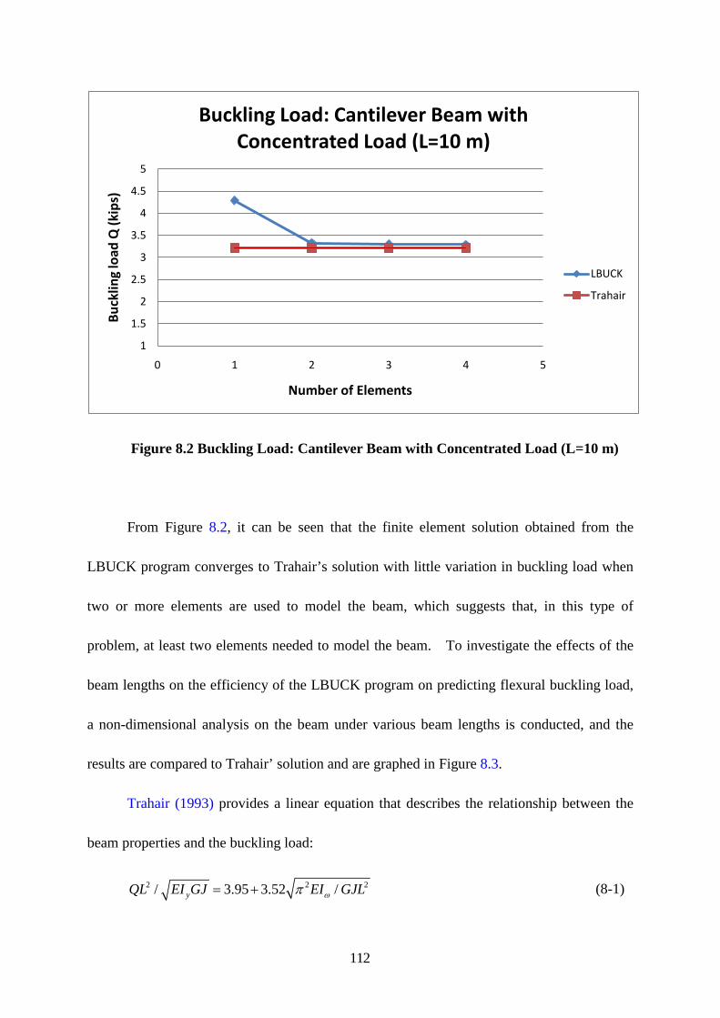
112
Figure 8.2 Buckling Load: Cantilever Beam with Concentrated Load (L=10 m)
From Figure 8.2, it can be seen that the finite element solution obtained from the
LBUCK program converges to Trahair’s solution with little variation in buckling load when
two or more elements are used to model the beam, which suggests that, in this type of
problem, at least two elements needed to model the beam. To investigate the effects of the
beam lengths on the efficiency of the LBUCK program on predicting flexural buckling load,
a non-dimensional analysis on the beam under various beam lengths is conducted, and the
results are compared to Trahair’ solution and are graphed in Figure 8.3.
Trahair (1993) provides a linear equation that describes the relationship between the
beam properties and the buckling load:
2 2 2/ 3.95 3.52 /yQL EI GJ EI GJLωπ= + (8-1)
1
1.5
2
2.5
3
3.5
4
4.5
5
0 1 2 3 4 5
Buck
ling
load
Q (k
ips)
Number of Elements
Buckling Load: Cantilever Beam with Concentrated Load (L=10 m)
LBUCK
Trahair
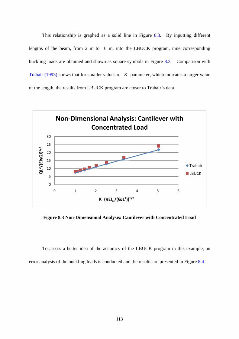
113
This relationship is graphed as a solid line in Figure 8.3. By inputting different
lengths of the beam, from 2 m to 10 m, into the LBUCK program, nine corresponding
buckling loads are obtained and shown as square symbols in Figure 8.3. Comparison with
Trahair (1993) shows that for smaller values of K parameter, which indicates a larger value
of the length, the results from LBUCK program are closer to Trahair’s data.
Figure 8.3 Non-Dimensional Analysis: Cantilever with Concentrated Load
To assess a better idea of the accuracy of the LBUCK program in this example, an
error analysis of the buckling loads is conducted and the results are presented in Figure 8.4.
0
5
10
15
20
25
30
0 1 2 3 4 5 6
QL2 /
(EIy
GJ)
1/2
K=(πEIω/(GJL2))1/2
Non-Dimensional Analysis: Cantilever withConcentrated Load
Trahair
LBUCK
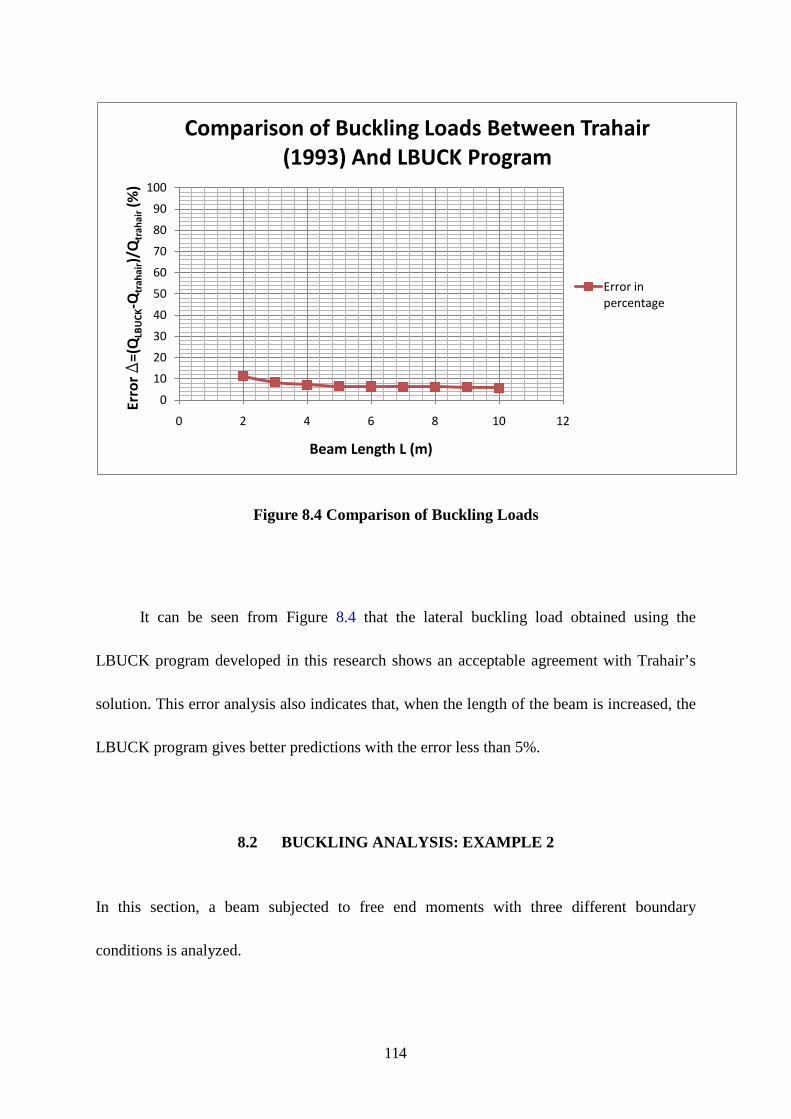
114
Figure 8.4 Comparison of Buckling Loads
It can be seen from Figure 8.4 that the lateral buckling load obtained using the
LBUCK program developed in this research shows an acceptable agreement with Trahair’s
solution. This error analysis also indicates that, when the length of the beam is increased, the
LBUCK program gives better predictions with the error less than 5%.
8.2 BUCKLING ANALYSIS: EXAMPLE 2
In this section, a beam subjected to free end moments with three different boundary
conditions is analyzed.
0
10
20
30
40
50
60
70
80
90
100
0 2 4 6 8 10 12
Erro
rD=(
QLB
UCK
-Qtr
ahai
r)/Q
trah
air(%
)
Beam Length L (m)
Comparison of Buckling Loads Between Trahair (1993) And LBUCK Program
Error in percentage
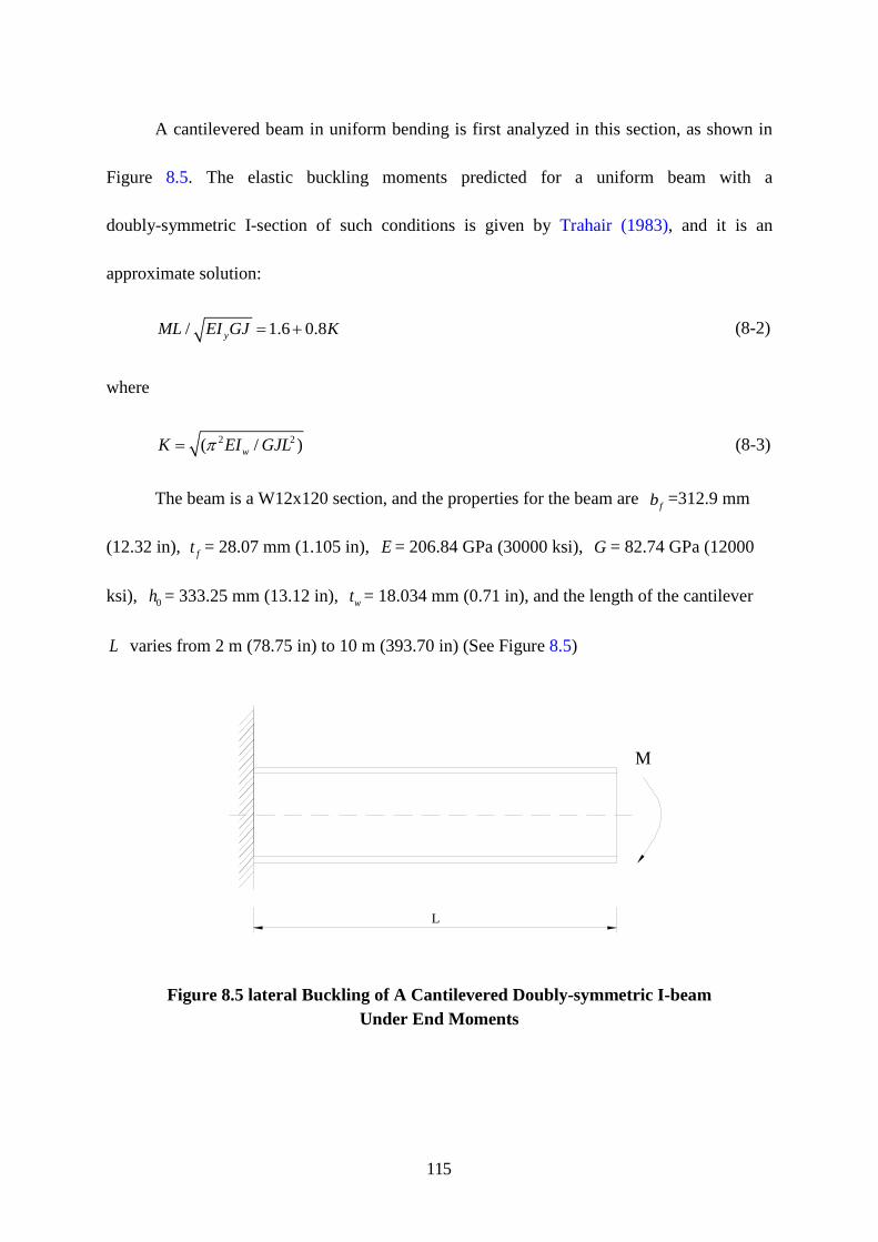
115
A cantilevered beam in uniform bending is first analyzed in this section, as shown in
Figure 8.5. The elastic buckling moments predicted for a uniform beam with a
doubly-symmetric I-section of such conditions is given by Trahair (1983), and it is an
approximate solution:
/ 1.6 0.8yML EI GJ K= + (8-2)
where
2 2( / )wK EI GJLπ= (8-3)
The beam is a W12x120 section, and the properties for the beam are fb =312.9 mm
(12.32 in), ft = 28.07 mm (1.105 in), E = 206.84 GPa (30000 ksi), G = 82.74 GPa (12000
ksi), 0h = 333.25 mm (13.12 in), wt = 18.034 mm (0.71 in), and the length of the cantilever
L varies from 2 m (78.75 in) to 10 m (393.70 in) (See Figure 8.5)
L
M
Figure 8.5 lateral Buckling of A Cantilevered Doubly-symmetric I-beam
Under End Moments
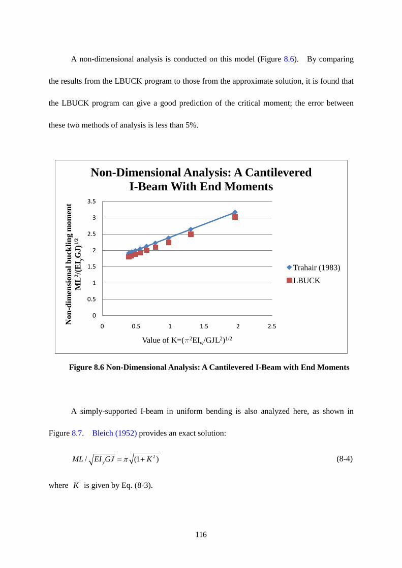
116
A non-dimensional analysis is conducted on this model (Figure 8.6). By comparing
the results from the LBUCK program to those from the approximate solution, it is found that
the LBUCK program can give a good prediction of the critical moment; the error between
these two methods of analysis is less than 5%.
Figure 8.6 Non-Dimensional Analysis: A Cantilevered I-Beam with End Moments
A simply-supported I-beam in uniform bending is also analyzed here, as shown in
Figure 8.7. Bleich (1952) provides an exact solution:
2/ (1 )yML EI GJ Kπ= + (8-4)
where K is given by Eq. (8-3).
0
0.5
1
1.5
2
2.5
3
3.5
0 0.5 1 1.5 2 2.5Non
-dim
ensi
onal
buc
klin
g m
omen
tM
L2 /(
EI y
GJ)
1/2
Value of K=(π2EIw/GJL2)1/2
Non-Dimensional Analysis: A Cantilevered I-Beam With End Moments
Trahair (1983)LBUCK
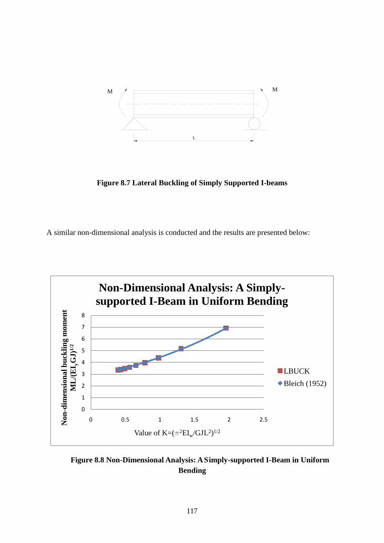
117
L
M M
Figure 8.7 Lateral Buckling of Simply Supported I-beams
A similar non-dimensional analysis is conducted and the results are presented below:
Figure 8.8 Non-Dimensional Analysis: A Simply-supported I-Beam in Uniform Bending
0
1
2
3
4
5
6
7
8
0 0.5 1 1.5 2 2.5Non
-dim
ensi
onal
buc
klin
g m
omen
tM
L/(E
I yG
J)1/
2
Value of K=(π2EIw/GJL2)1/2
Non-Dimensional Analysis: A Simply-supported I-Beam in Uniform Bending
LBUCKBleich (1952)
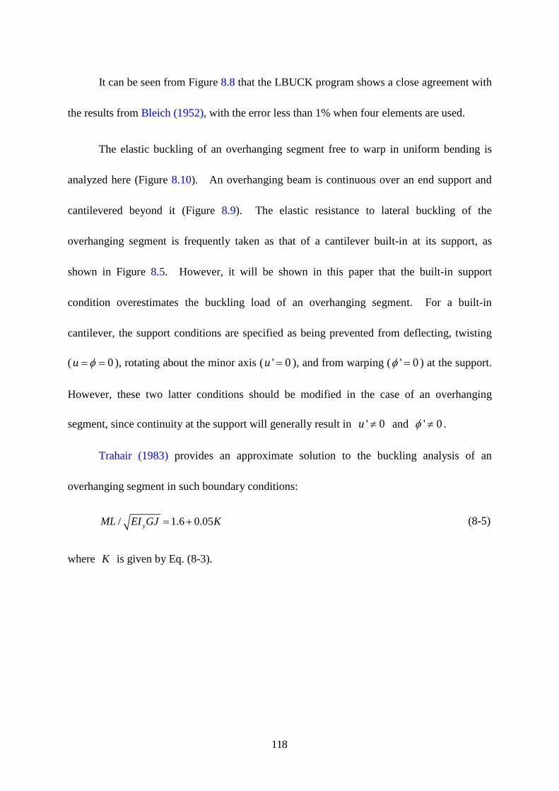
118
It can be seen from Figure 8.8 that the LBUCK program shows a close agreement with
the results from Bleich (1952), with the error less than 1% when four elements are used.
The elastic buckling of an overhanging segment free to warp in uniform bending is
analyzed here (Figure 8.10). An overhanging beam is continuous over an end support and
cantilevered beyond it (Figure 8.9). The elastic resistance to lateral buckling of the
overhanging segment is frequently taken as that of a cantilever built-in at its support, as
shown in Figure 8.5. However, it will be shown in this paper that the built-in support
condition overestimates the buckling load of an overhanging segment. For a built-in
cantilever, the support conditions are specified as being prevented from deflecting, twisting
( 0u φ= = ), rotating about the minor axis ( ' 0u = ), and from warping ( ' 0φ = ) at the support.
However, these two latter conditions should be modified in the case of an overhanging
segment, since continuity at the support will generally result in ' 0u ≠ and ' 0φ ≠ .
Trahair (1983) provides an approximate solution to the buckling analysis of an
overhanging segment in such boundary conditions:
/ 1.6 0.05yML EI GJ K= + (8-5)
where K is given by Eq. (8-3).
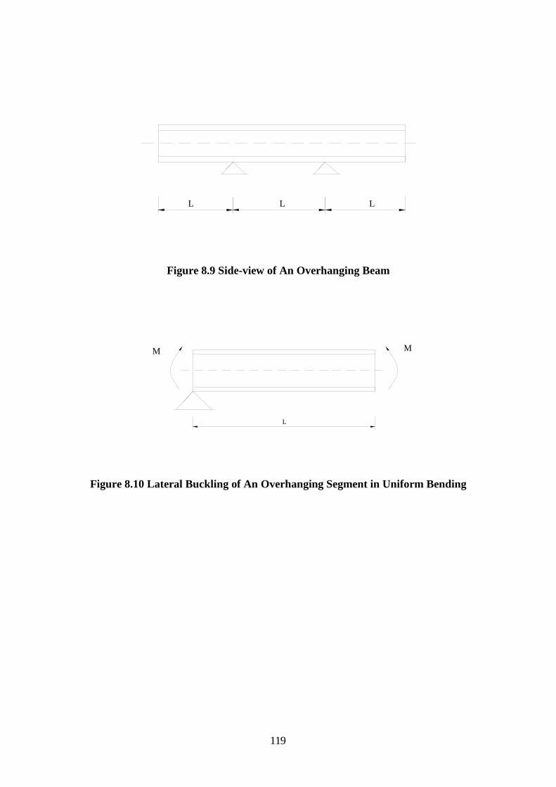
119
LL L
Figure 8.9 Side-view of An Overhanging Beam
L
M M
Figure 8.10 Lateral Buckling of An Overhanging Segment in Uniform Bending
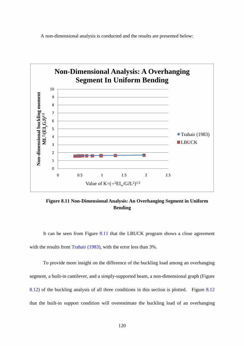
120
A non-dimensional analysis is conducted and the results are presented below:
Figure 8.11 Non-Dimensional Analysis: An Overhanging Segment in Uniform Bending
It can be seen from Figure 8.11 that the LBUCK program shows a close agreement
with the results from Trahair (1983), with the error less than 3%.
To provide more insight on the difference of the buckling load among an overhanging
segment, a built-in cantilever, and a simply-supported beam, a non-dimensional graph (Figure
8.12) of the buckling analysis of all three conditions in this section is plotted. Figure 8.12
that the built-in support condition will overestimate the buckling load of an overhanging
0
1
2
3
4
5
6
7
8
9
10
0 0.5 1 1.5 2 2.5
Non
-dim
ensi
onal
buc
klin
g m
omen
tM
L2 /(
EI y
GJ)
1/2
Value of K=(π2EIw/GJL2)1/2
Non-Dimensional Analysis: A Overhanging Segment In Uniform Bending
Trahair (1983)LBUCK
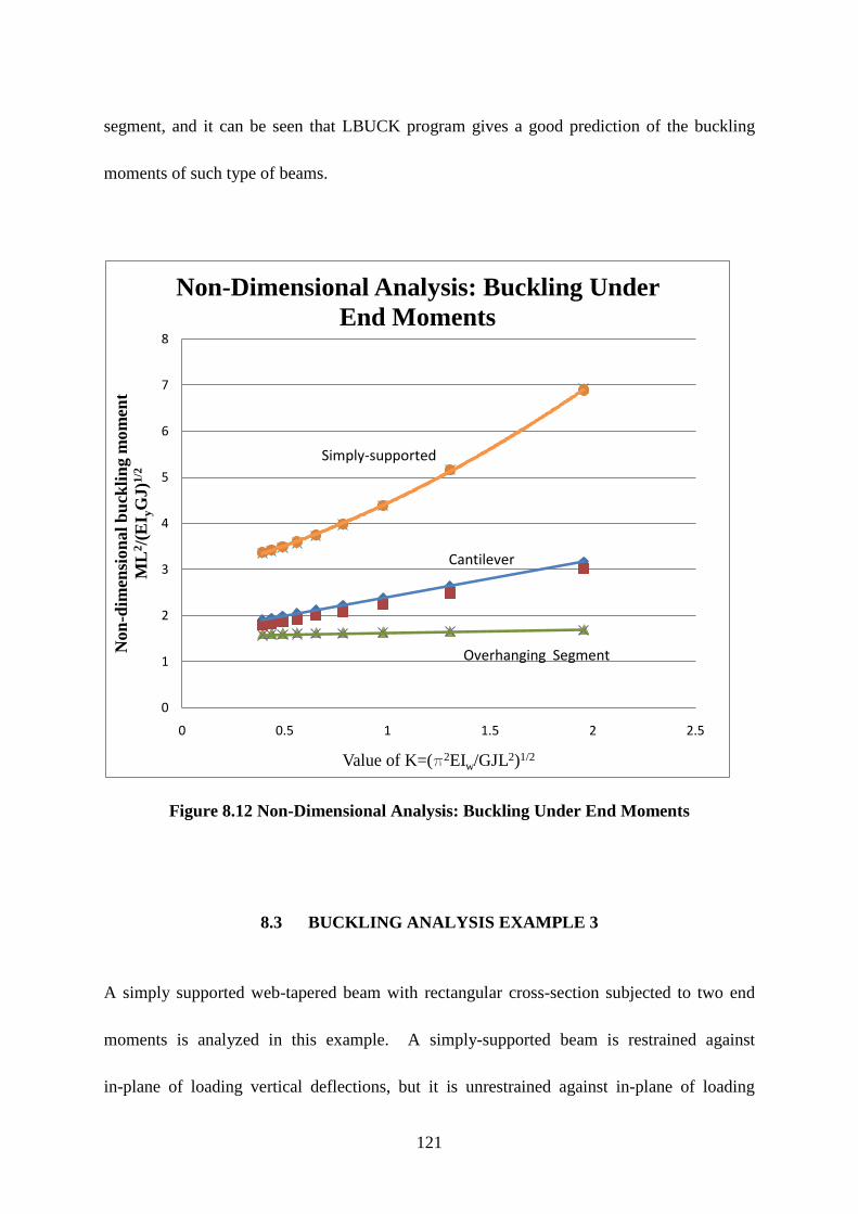
121
segment, and it can be seen that LBUCK program gives a good prediction of the buckling
moments of such type of beams.
Figure 8.12 Non-Dimensional Analysis: Buckling Under End Moments
8.3 BUCKLING ANALYSIS EXAMPLE 3
A simply supported web-tapered beam with rectangular cross-section subjected to two end
moments is analyzed in this example. A simply-supported beam is restrained against
in-plane of loading vertical deflections, but it is unrestrained against in-plane of loading
0
1
2
3
4
5
6
7
8
0 0.5 1 1.5 2 2.5
Non
-dim
ensi
onal
buc
klin
g m
omen
tM
L2 /(
EI y
GJ)
1/2
Value of K=(π2EIw/GJL2)1/2
Non-Dimensional Analysis: Buckling Under End Moments
Simply-supported
Cantilever
Overhanging Segment
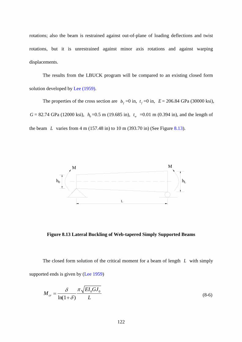
122
rotations; also the beam is restrained against out-of-plane of loading deflections and twist
rotations, but it is unrestrained against minor axis rotations and against warping
displacements.
The results from the LBUCK program will be compared to an existing closed form
solution developed by Lee (1959).
The properties of the cross section are fb =0 in, ft =0 in, E = 206.84 GPa (30000 ksi),
G = 82.74 GPa (12000 ksi), 0h =0.5 m (19.685 in), wt =0.01 m (0.394 in), and the length of
the beam L varies from 4 m (157.48 in) to 10 m (393.70 in) (See Figure 8.13).
L
M M
h0 hL
Figure 8.13 Lateral Buckling of Web-tapered Simply Supported Beams
The closed form solution of the critical moment for a beam of length L with simply
supported ends is given by (Lee 1959)
0 0
ln(1 )cr
EI GJM
Lπδ
δ=
+ (8-6)
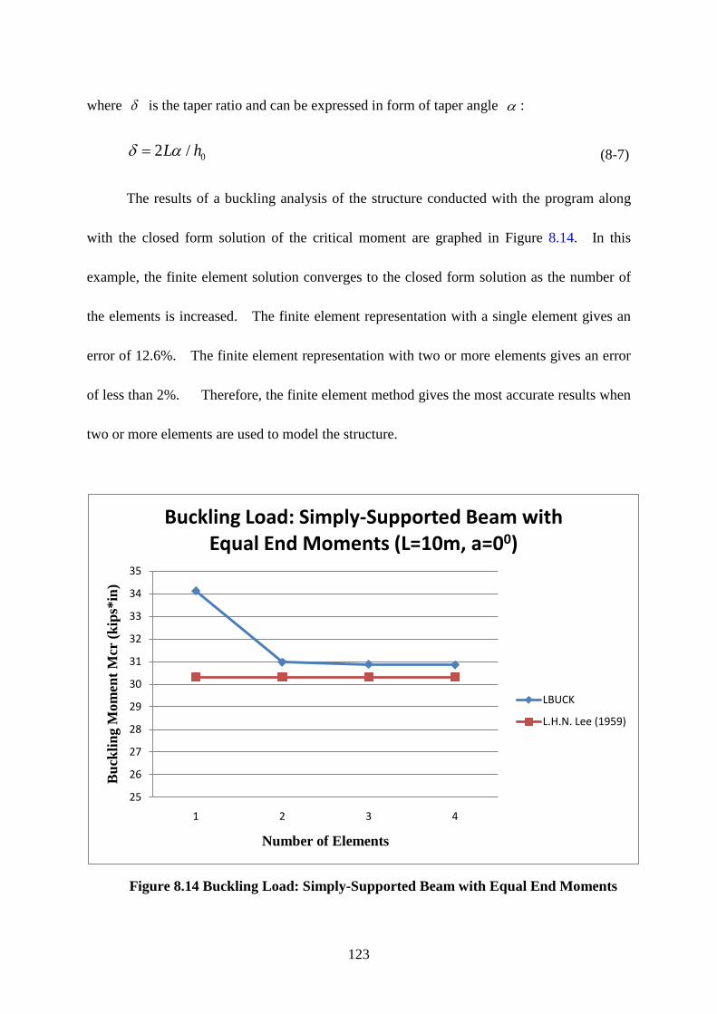
123
where δ is the taper ratio and can be expressed in form of taper angle α :
02 /L hδ α= (8-7)
The results of a buckling analysis of the structure conducted with the program along
with the closed form solution of the critical moment are graphed in Figure 8.14. In this
example, the finite element solution converges to the closed form solution as the number of
the elements is increased. The finite element representation with a single element gives an
error of 12.6%. The finite element representation with two or more elements gives an error
of less than 2%. Therefore, the finite element method gives the most accurate results when
two or more elements are used to model the structure.
Figure 8.14 Buckling Load: Simply-Supported Beam with Equal End Moments
25
26
27
28
29
30
31
32
33
34
35
1 2 3 4
Buc
klin
g M
omen
t Mcr
(kip
s*in
)
Number of Elements
Buckling Load: Simply-Supported Beam with Equal End Moments (L=10m, a=00)
LBUCK
L.H.N. Lee (1959)
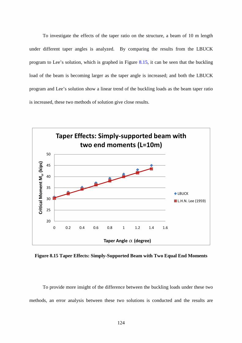
124
To investigate the effects of the taper ratio on the structure, a beam of 10 m length
under different taper angles is analyzed. By comparing the results from the LBUCK
program to Lee’s solution, which is graphed in Figure 8.15, it can be seen that the buckling
load of the beam is becoming larger as the taper angle is increased; and both the LBUCK
program and Lee’s solution show a linear trend of the buckling loads as the beam taper ratio
is increased, these two methods of solution give close results.
Figure 8.15 Taper Effects: Simply-Supported Beam with Two Equal End Moments
To provide more insight of the difference between the buckling loads under these two
methods, an error analysis between these two solutions is conducted and the results are
20
25
30
35
40
45
50
0 0.2 0.4 0.6 0.8 1 1.2 1.4 1.6
Crit
ical
Mom
ent
Mcr
(kip
s)
Taper Angle a (degree)
Taper Effects: Simply-supported beam with two end moments (L=10m)
LBUCK
L.H.N. Lee (1959)
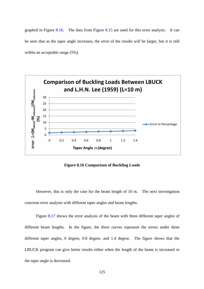
125
graphed in Figure 8.16. The data from Figure 8.15 are used for this error analysis. It can
be seen that as the taper angle increases, the error of the results will be larger, but it is still
within an acceptable range (5%).
Figure 8.16 Comparison of Buckling Loads
However, this is only the case for the beam length of 10 m. The next investigation
concerns error analysis with different taper angles and beam lengths.
Figure 8.17 shows the error analysis of the beam with three different taper angles of
different beam lengths. In the figure, the three curves represent the errors under three
different taper angles, 0 degree, 0.8 degree, and 1.4 degree. The figure shows that the
LBUCK program can give better results either when the length of the beam is increased or
the taper angle is decreased.
0
5
10
15
20
25
30
0 0.2 0.4 0.6 0.8 1 1.2 1.4
Erro
r D
=(M
LBU
CK-M
refe
rece
)/M
refe
renc
e
(%)
Taper Angle a(degree)
Comparison of Buckling Loads Between LBUCK and L.H.N. Lee (1959) (L=10 m)
Error in Percentage
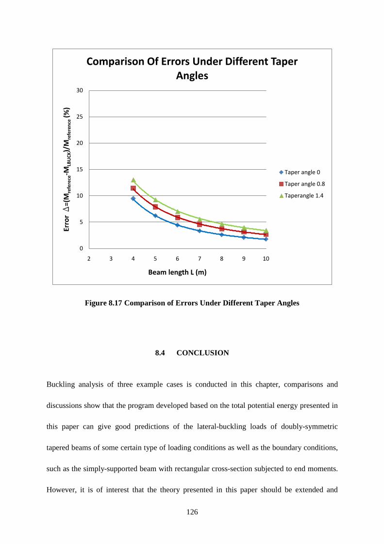
126
Figure 8.17 Comparison of Errors Under Different Taper Angles
8.4 CONCLUSION
Buckling analysis of three example cases is conducted in this chapter, comparisons and
discussions show that the program developed based on the total potential energy presented in
this paper can give good predictions of the lateral-buckling loads of doubly-symmetric
tapered beams of some certain type of loading conditions as well as the boundary conditions,
such as the simply-supported beam with rectangular cross-section subjected to end moments.
However, it is of interest that the theory presented in this paper should be extended and
0
5
10
15
20
25
30
2 3 4 5 6 7 8 9 10
Erro
r D
=(M
refe
rece
-MLB
UCK
)/M
refe
renc
e(%
)
Beam length L (m)
Comparison Of Errors Under Different Taper Angles
Taper angle 0
Taper angle 0.8
Taperangle 1.4

127
applied to more general cases, such as tapered beams of I-sections subjected to distributed
loading or more complex boundary conditions, and the effects of the loadings on the buckling
loads of the beams remains to be investigated in the future research.
128
9.0 SUMMARY
Theoretical analysis of flexural-torsional buckling of doubly-symmetric web-tapered I-beams
using finite element method is mainly investigated in this study. The first two chapters
present an introduction to the topic and a review of existing literatures. Chapter 3 presents
the derivation of the total potential energy equations. Chapter 4 verifies the validity of the
transformation equation to derive the cross section properties compared to those from the
reference. Chapter 5 implements the finite element method into the total potential energy
equation, and Chapter 6 explains the eigenvalue solution procedure to a generalized matrix
problem. Chapter 7 introduces the concept of object-oriented technology and software
development. Three example cases are analyzed in Chapter 8. And the following
paragraph is a summary and findings of this research.
To calculate the flexural-torsional buckling load of a doubly-symmetric web-tapered
I-beam, the study began with the derivation of the energy equations. The total potential
energy equation was derived for the flexural-torsional buckling of a beam element by
summing up the strain energy and the potential energy of the external loads. The first
variation of the total potential energy equals to zero is the statement of the minimum total
potential energy. The second variation of the total potential energy equals to zero indicates
the transition from a stable to an unstable configuration. The development of the theory in
129
this research is based on the second variation of the total potential energy. The finite
element method is then implemented into the energy equations to derive the element elastic
stiffness and geometric stiffness matrices of a doubly-symmetric web-tapered beam element.
Cubic polynomials were assumed for the displacement functions. Due to the tapered effects,
the web-tapered I-beam element is synthesized into three parts, the top flange, the web, and
the bottom flange. Some transformation matrices were developed based on geometry to
convert the energy equations of the flanges in their own coordinate systems to the web
coordinate system. The stiffness matrices then can be formulated for an individual
web-tapered I-beam element. Stiffness matrices of individual elements in global
coordinates were then summed up to provide the stiffness and geometric stiffness matrices of
a beam consisting of several elements.
The final equation for calculating the flexural-torsional buckling loads is in the form of
a generalized eigenvalue problem. It is converted to a standard eigenvalue equation using
the Cholesky method. Householder’s method is then used to change the standard matrix
into a tridiagonal matrix. The eigenvalue of the tridiagonal matrix was calculated using QL
iteration. The buckling parameter is the inverse of the smallest eigenvalue.
Computer technology was utilized due to the compatibility of finite element method
with software. An existing software that has used the finite element equations of a
beam-column element to calculate the flexural-torsional buckling loads of a plane frame
structure is refactored. The contents of the program are modified to meet current needs.
130
The original program was not object-oriented and not user friendly. Object-oriented
technology was applied to the existing flexural-torsional buckling program by refactoring the
existing program. First, the basic system requirements were determined. Next, models
were created considering object-oriented concepts to communicate with the new software
structure. The models considered included the user case diagram, the class diagram, the
sequence diagram, and the activity diagram. Then, the program code was changed from an
older procedural structure to an object-oriented structure reflecting the object-oriented models.
Object-oriented software development is a useful tool in engineering applications to increase
the flexibility of the software applications. An object-oriented design of an existing
flexural-torsional buckling analysis program was presented in this study.
In Chapter 8, three example cases were analyzed to compare the results from the
software package to the existing theoretical solutions. The finite element method always
predicts a buckling factor that is larger than the actual value from an existing closed form
solution. To increase the accuracy of the finite element solution, more elements are needed
to model the beam. The examples show that the program can provide reasonable results
when at least two elements are used, and they also show that the program developed based
upon the theory proposed provides good results when analyzing the beams as presented in
Chapter 8, which encourages the further research on more complex situations.
Further research remains to be the development of the program based on the theory
that can investigate the flexural-torsional buckling of doubly-symmetric web-tapered I-beam.
The research of interest should be: the effects of loading position on the buckling load, the

131
flexural-torsional buckling load of web-tapered I-beam subjected to more complex loading
conditions, e.g., distributed loading, combination of distributed load with concentrated loads,
as well as more complex boundary conditions, e.g., continuous beams, frame structures.
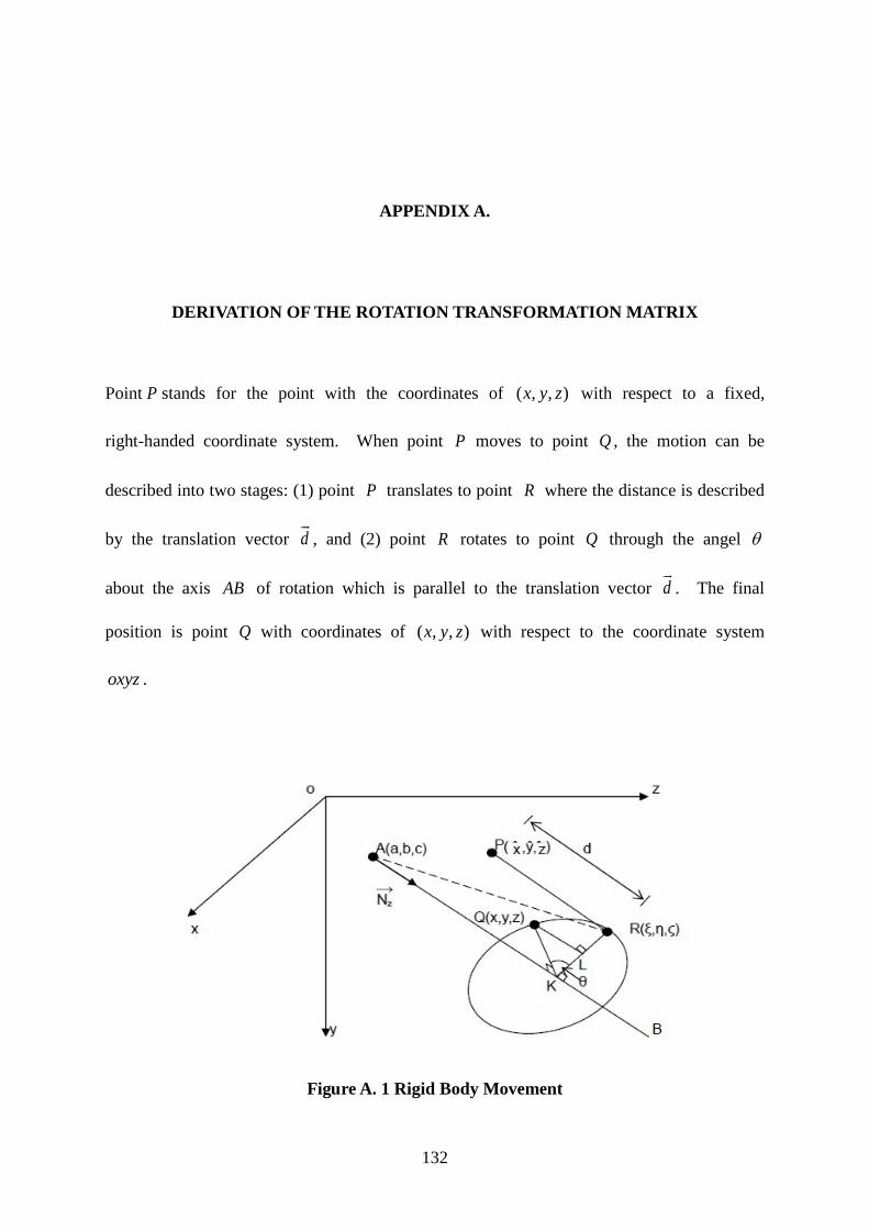
132
APPENDIX A.
DERIVATION OF THE ROTATION TRANSFORMATION MATRIX
Point P stands for the point with the coordinates of ( , , )x y z with respect to a fixed,
right-handed coordinate system. When point P moves to point Q , the motion can be
described into two stages: (1) point P translates to point R
where the distance is described
by the translation vector d
, and (2) point R rotates to point Q
through the angel θ
about the axis AB of rotation which is parallel to the translation vector d
. The final
position is point Q with coordinates of ( , , )x y z
with respect to the coordinate system
oxyz .
Figure A. 1 Rigid Body Movement
133
The objective of this Appendix is to show that the coordinates of the point Q can be
calculated from the coordinate of the point P , the component of a translation vector d
and
direction cosines of the axis of rotation AB .
The axis of rotation AB passes through the point c, which has coordinates ( , , )a b c
and has direction-angles of α , β , and γ with respect to the oxyz coordinate system.
Points Q and R are located in a plane perpendicular to the line AB . A unit vector N
on the axis of rotation AB has the same directional cosines as the rotation angle θ
and is
given by
cos cos cosN i j kα β γ= + +
(A-1)
The vector oQ
can be broken into its vector components expressed by
oQ oR RL LQ= + +
(A-2)
Therefore, the vector oQ
may be found by determining each of its components, oR
,
RL
, and LQ
in terms of the coordinates of point P , the components of a translation vector
d
, direction cosines of the axis of rotation AB , and rotational angle θ .
A. 1 VECTOR oR
The point P translates to the point R with coordinates ( , , )ε η ζ with respect to the oxyz
coordinate system. The coordinate of point R may be expressed in terms of the coordinates
of point P and the translation vector d
as
134
^
cosx dξ α= +
(A-3)
^
cosy dη β= +
(A-4)
^
cosz dζ γ= +
(A-5)
A. 2 VECTOR RL
The point K shown in Figure A.1 is the projection of points R and Q on the axis AB .
The vectors KR and KQ are equal in magnitude and are radii of the rotation about AB ,
where the rotation angle, θ , is the angle ^
R K Q . The point L shown in Figure A.1 is the
projection of the point Q on the line KR . The vector KR
may be defined as
KR AR AK= −
(A-6)
And it can be expanded as
[( ) ( ) ( ) ]KR a i b j c k AKξ η ζ= − + − + − −
(A-7)
Vector AK
is the projection of AR
on line AB . Therefore,
( )AK AR N N= ⋅
(A-8)
By considering the components of vectors AR
and N
, Eq. (A-8) may be expressed as
[( ) cos ( ) cos ( ) cos ](cos cos cos )AK a b c i j kξ α η β ζ γ α β γ= − + − + − + +
(A-9)
135
Substituting Eq. (A-9) into (A-7) gives
[( ) cos (( ) cos ( ) cos ( ) cos )]KR a a b c iξ α ξ α η β ζ γ= − − − + − + −
+[( ) cos (( ) cos ( ) cos ( ) cos )]b a b c jη β ξ α η β ζ γ− − − + − + −
+[( ) cos (( ) cos ( ) cos ( ) cos )]c a b c kζ γ ξ α η β ζ γ− − − + − + −
(A-10)
The vector RL
may be written as
RL RK LK= −
(A-11)
cosRL KR KR θ= − +
(A-12)
(1 cos )RL KRθ= − −
(A-13)
Substituting Eq. (A-10) into Eq. (A-13) gives
(1 cos )[( ) cos (( ) cos ( ) cos ( ) cos )]RL a a b c iθ ξ α ξ α η β ζ γ= − − − − − + − + −
(1 cos )[( ) cos (( ) cos ( ) cos ( ) cos )]b a b c jθ η β ξ α η β ζ γ− − − − − + − + −
(1 cos )[( ) cos (( ) cos ( ) cos ( ) cos )]c a b c kθ ζ γ ξ α η β ζ γ− − − − − + − + −
(A-14)
A. 3 VECTOR LQ
By definition of vector cross-product
[( ) cos ( ) cos ] [( ) cos ( ) cos ]N AR c b i a c jζ β η γ ξ γ ζ α× = − − − + − − −
[( ) cos ( ) cos ]b a kη α ξ β+ − − −
(A-15)
136
And
^
| | sinN AR AR K A R× =
(A-16)
From triangle ARK ,
^
sinAR K A R KR= (A-17)
Therefore,
| |N AR KR× =
(A-18)
A unit vector, LQN
, in the direction LQ is defined as
| |LQN ARNN AR×
=×
(A-19)
Substituting Eq. (A-18) into (A-19) gives
LQ
N ARNKR×
=
(A-20)
Substituting Eq. (A-15) into Eq. (A-20) gives
1 [( ) cos ( ) cos ] [( ) cos ( ) cos ]LQN c b i a c jKR
ζ β η γ ξ γ ζ α= − − − + − − −
[( ) cos ( ) cos ] b a kη α ξ β+ − − −
(A-21)
Since
sin sinLQ KQ KRθ θ= = (A-22)
The vector LQ
may be expressed as
sin LQLQ KR Nθ=
(A-23)
137
From Eq. (A-21) and (A-23), the vector LQ
may be written as
sin [( ) cos ( ) cos ] [( ) cos ( ) cos ]LQ c b i a c jθ ζ β η γ ξ γ ζ α= − − − + − − −
[( ) cos ( ) cos ] b a kη α ξ β+ − − −
(A-24)
A. 4 FINITE DISPLACEMENTS TRANSFORMATION
To define the finite displacements transformation matrix, consider the x y and z components
of Eq. (A-2) in the form of
x xx RL LQξ= + + (A-25a)
y yy RL LQη= + + (A-25b)
z zz RL LQζ= + + (A-25c)
Substituting in for vectors RL
from Eq. (A-14) and LQ
from Eq. (A-24) into (A-25a) to
(A-25c) gives
2(1 cos )[( ) ( ) cos ( ) cos cos ( )cos cos ]x a a b a cξ θ ξ ξ α η β ζ α γ= − − − − − − − − −
sin [( ) cos ( ) cos ]c bθ ξ β η γ+ − − − (A-26a)
2(1 cos )[( ) ( ) cos cos ( )cos ( ) cos cos ]y b a b cη θ η ξ α β η β ζ β γ= − − − − − − − − −
sin [( ) cos ( ) cos ]a cθ ξ γ ζ α+ − − − (A-26b)
2(1 cos )[( ) ( ) cos cos ( )cos cos ( )cos ]z c a b cζ θ ζ ξ α γ η β γ ζ γ= − − − − − − − − −
sin [( ) cos ( ) cos ]b aθ η α ξ β+ − − − (A-26c)
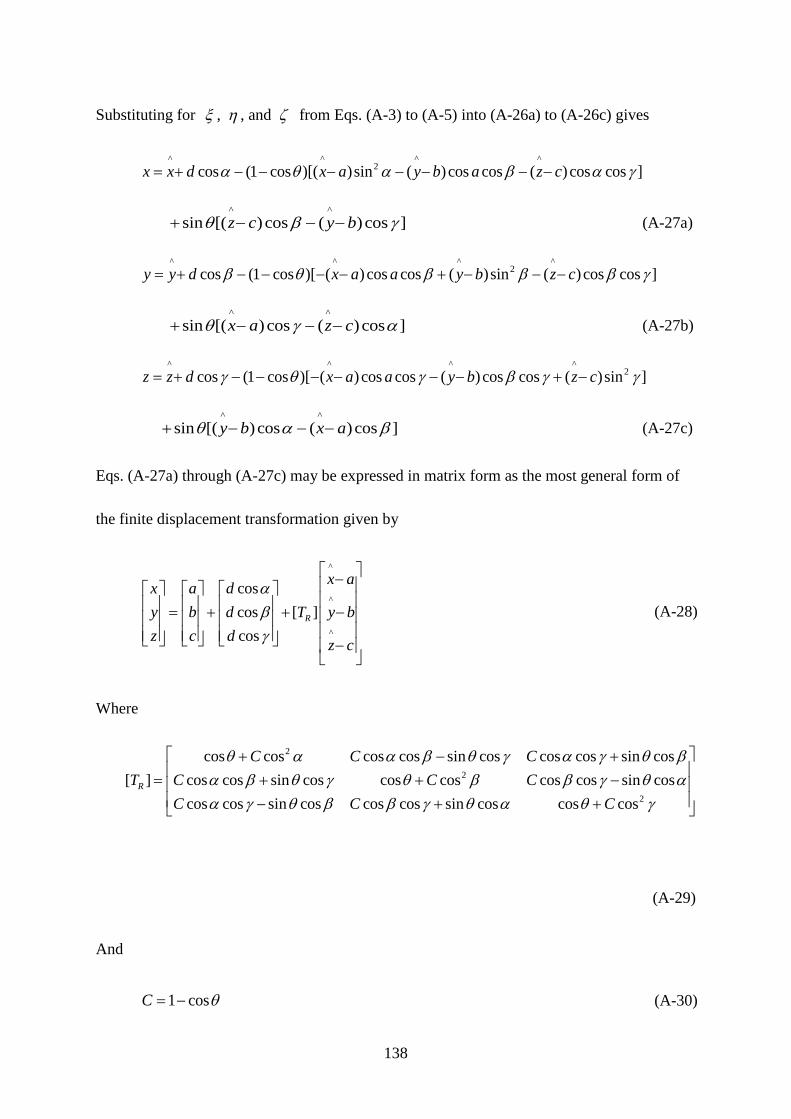
138
Substituting for ξ , η , and ζ from Eqs. (A-3) to (A-5) into (A-26a) to (A-26c) gives
^ ^ ^ ^
2cos (1 cos )[( )sin ( ) cos cos ( )cos cos ]x x d x a y b a z cα θ α β α γ= + − − − − − − −
^ ^
sin [( ) cos ( ) cos ]z c y bθ β γ+ − − − (A-27a)
^ ^ ^ ^
2cos (1 cos )[ ( ) cos cos ( )sin ( ) cos cos ]y y d x a a y b z cβ θ β β β γ= + − − − − + − − −
^ ^sin [( ) cos ( ) cos ]x a z cθ γ α+ − − − (A-27b)
^ ^ ^ ^
2cos (1 cos )[ ( ) cos cos ( )cos cos ( )sin ]z z d x a a y b z cγ θ γ β γ γ= + − − − − − − + −
^ ^sin [( ) cos ( ) cos ]y b x aθ α β+ − − − (A-27c)
Eqs. (A-27a) through (A-27c) may be expressed in matrix form as the most general form of
the finite displacement transformation given by
^
^
^
coscos [ ]cos
R
x ax a dy b d T y bz c d z c
αβγ
− = + + − −
(A-28)
Where
2
2
2
cos cos cos cos sin cos cos cos sin cos[ ] cos cos sin cos cos cos cos cos sin cos
cos cos sin cos cos cos sin cos cos cosR
C C CT C C C
C C C
θ α α β θ γ α γ θ βα β θ γ θ β β γ θ αα γ θ β β γ θ α θ γ
+ − + = + + − − + +
(A-29)
And
1 cosC θ= − (A-30)
139
A.5 ROTATION TRANSFORMATION MATRIX
For small rotation transformation, we have d
=0; therefore, Eqs. (A-3) to (A-5) can be
simplified to
^xξ = (A-31a)
^yη = (A-31b)
^zζ = (A-31c)
Using Eqs. (A-31) in (A-26), we have
^ ^ ^ ^
2(1 cos )[( )sin ( ) cos cos ( )cos cos ]x x x a y b a z cθ α β α γ= − − − − − − −
^ ^sin [( ) cos ( ) cos ]z c y bθ β γ+ − − − (A-32a)
^ ^ ^ ^
2(1 cos )[( )sin ( ) cos cos ( )cos cos ]y y y b x a z cθ β α β β γ= − − − − − − −
^ ^sin [( ) cos ( ) cos ]x a z cθ γ α+ − − − (A-32b)
^ ^ ^ ^
2(1 cos )[( )sin ( ) cos cos ( )cos cos ]z z z c x a y bθ γ α γ β γ= − − − − − − −
^ ^sin [( ) cos ( ) cos ]y b x aθ α β+ − − − (A-32c)
If the rotation axis AB passes through the origin, then 0a b c= = = , and Eqs. (A-32) can
be simplified to
^ ^ ^ ^ ^ ^
2(1 cos )[ sin cos cos cos cos ] sin [ cos cos ]x x x y a z z yθ α β α γ θ β γ= − − − − + −
(A-33a)
140
^ ^ ^ ^ ^ ^
2(1 cos )[ sin cos cos cos cos ] sin [ cos cos ]y y y x a z x zθ β β β γ θ γ α= − − − − + −
(A-33b)
^ ^ ^ ^ ^ ^
2(1 cos )[ sin cos cos cos cos ] sin [ cos cos ]z z z x a y y xθ γ γ β γ θ α β= − − − − + −
(A-33c)
Eqs. (A-33) may be simplified using trigonometric identities and expressed as
^ ^ ^ ^ ^ ^2 22sin [ sin cos cos cos cos ] 2sin cos [ cos cos ]
2 2 2x x x y a z z yθ θ θα β α γ β γ= − − − + −
(A-34a)
^ ^ ^ ^ ^ ^2 22sin [ sin cos cos cos cos ] 2sin cos [ cos cos ]
2 2 2y y y x a z x zθ θ θβ β β γ γ α= − − − + −
(A-34b)
^ ^ ^ ^ ^ ^2 22sin [ sin cos cos cos cos ] 2sin cos [ cos cos ]
2 2 2z z z x a y y xθ θ θγ γ β γ α β= − − − + −
(A-34c)
Eqs. (A-34) may be expressed in the following form
^ ^2 2 2(1 2sin sin ) (2sin cos cos 2sin cos cos )
2 2 2 2x x yθ θ θ θα α β γ= − + −
^2(2sin cos cos 2sin cos cos )
2 2 2zθ θ θα γ β+ + (A-35a)
^ ^2 2 2(2sin cos cos 2sin cos cos ) (1 2sin sin )
2 2 2 2y x yθ θ θ θα β γ β= + + −
^2(2sin cos cos 2sin cos cos )
2 2 2zθ θ θβ γ α+ − (A-35b)
^ ^2 2(2sin cos cos 2sin cos cos ) (2sin cos cos 2sin cos cos )
2 2 2 2 2 2z x yθ θ θ θ θ θα γ β β γ α= − + +
^2 2(1 2sin sin )
2zθ γ+ − (A-35c)
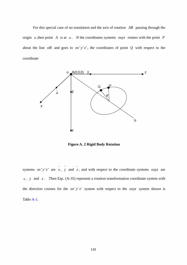
141
For this special case of no translation and the axis of rotation AB passing through the
origin o ,then point A is at o . If the coordinates systems oxyz rotates with the point P
about the line oB and goes to ' ' 'ox y z , the coordinates of point Q with respect to the
coordinate
Figure A. 2 Rigid Body Rotation
systems ' ' 'ox y z are ^x ,
^y and
^z , and with respect to the coordinate systems oxyz are
x , y and z . Then Eqs. (A-35) represent a rotation transformation coordinate system with
the direction cosines for the ' ' 'ox y z system with respect to the oxyz system shown is
Table A-1.
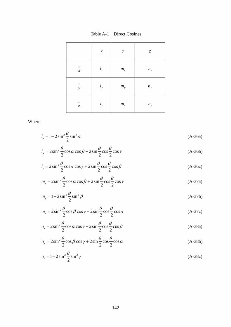
142
Table A-1 Direct Cosines
x y z
^x xl xm xn
^y yl ym yn
^z zl zm zn
Where
2 21 2sin sin
2xlθ α= − (A-36a)
22sin cos cos 2sin cos cos
2 2 2ylθ θ θα β γ= − (A-36b)
22sin cos cos 2sin cos cos
2 2 2zlθ θ θα γ β= + (A-36c)
22sin cos cos 2sin cos cos
2 2 2xm θ θ θα β γ= + (A-37a)
2 21 2sin sin
2ym θ β= − (A-37b)
22sin cos cos 2sin cos cos
2 2 2zm θ θ θβ γ α= − (A-37c)
22sin cos cos 2sin cos cos
2 2 2xn θ θ θα γ β= − (A-38a)
22sin cos cos 2sin cos cos
2 2 2yn θ θ θβ γ α= + (A-38b)
2 21 2sin sin
2zn θ γ= − (A-38c)
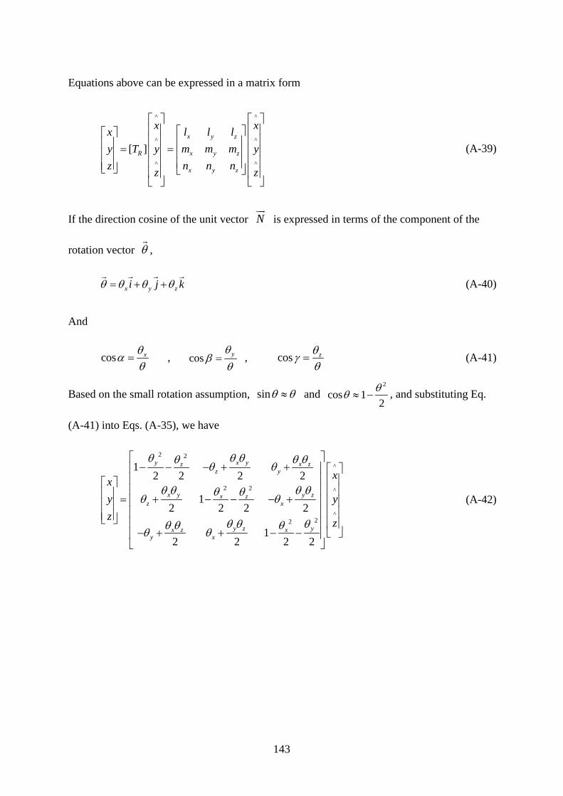
143
Equations above can be expressed in a matrix form
^ ^
^ ^
^ ^
[ ]x y z
R x y z
x y z
x xx l l ly T y m m m yz n n nz z
= =
(A-39)
If the direction cosine of the unit vector N
is expressed in terms of the component of the
rotation vector θ
,
x y zi j kθ θ θ θ= + +
(A-40)
And
cos xθα
θ= , cos yθβ
θ= , cos zθγ
θ= (A-41)
Based on the small rotation assumption, sinθ θ≈ and 2
cos 12θθ ≈ − , and substituting Eq.
(A-41) into Eqs. (A-35), we have
2 2^
2 2 ^
^22
12 2 2 2
12 2 2 2
12 2 2 2
y x y x zzz y
x y y zx zz x
y z yx z xy x
xxy yz z
θ θ θ θ θθ θ θ
θ θ θ θθ θθ θ
θ θ θθ θ θθ θ
− − − + +
= + − − − + − + + − −
(A-42)
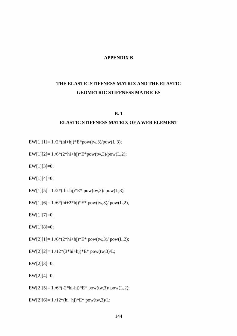
144
APPENDIX B
THE ELASTIC STIFFNESS MATRIX AND THE ELASTIC
GEOMETRIC STIFFNESS MATRICES
B. 1
ELASTIC STIFFNESS MATRIX OF A WEB ELEMENT
EW[1][1]= 1./2*(hi+hj)*E*pow(tw,3)/pow(L,3);
EW[1][2]= 1./6*(2*hi+hj)*E*pow(tw,3)/pow(L,2);
EW[1][3]=0;
EW[1][4]=0;
EW[1][5]= 1./2*(-hi-hj)*E* pow(tw,3)/ pow(L,3),
EW[1][6]= 1./6*(hi+2*hj)*E* pow(tw,3)/ pow(L,2),
EW[1][7]=0,
EW[1][8]=0;
EW[2][1]= 1./6*(2*hi+hj)*E* pow(tw,3)/ pow(L,2);
EW[2][2]= 1./12*(3*hi+hj)*E* pow(tw,3)/L;
EW[2][3]=0;
EW[2][4]=0;
EW[2][5]= 1./6*(-2*hi-hj)*E* pow(tw,3)/ pow(L,2);
EW[2][6]= 1./12*(hi+hj)*E* pow(tw,3)/L;
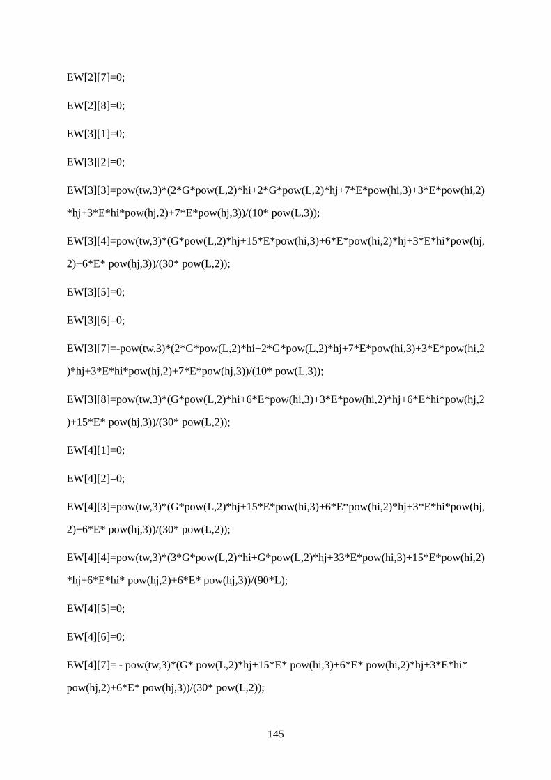
145
EW[2][7]=0;
EW[2][8]=0;
EW[3][1]=0;
EW[3][2]=0;
EW[3][3]=pow(tw,3)*(2*G*pow(L,2)*hi+2*G*pow(L,2)*hj+7*E*pow(hi,3)+3*E*pow(hi,2)
*hj+3*E*hi*pow(hj,2)+7*E*pow(hj,3))/(10* pow(L,3));
EW[3][4]=pow(tw,3)*(G*pow(L,2)*hj+15*E*pow(hi,3)+6*E*pow(hi,2)*hj+3*E*hi*pow(hj,
2)+6*E* pow(hj,3))/(30* pow(L,2));
EW[3][5]=0;
EW[3][6]=0;
EW[3][7]=-pow(tw,3)*(2*G*pow(L,2)*hi+2*G*pow(L,2)*hj+7*E*pow(hi,3)+3*E*pow(hi,2
)*hj+3*E*hi*pow(hj,2)+7*E*pow(hj,3))/(10* pow(L,3));
EW[3][8]=pow(tw,3)*(G*pow(L,2)*hi+6*E*pow(hi,3)+3*E*pow(hi,2)*hj+6*E*hi*pow(hj,2
)+15*E* pow(hj,3))/(30* pow(L,2));
EW[4][1]=0;
EW[4][2]=0;
EW[4][3]=pow(tw,3)*(G*pow(L,2)*hj+15*E*pow(hi,3)+6*E*pow(hi,2)*hj+3*E*hi*pow(hj,
2)+6*E* pow(hj,3))/(30* pow(L,2));
EW[4][4]=pow(tw,3)*(3*G*pow(L,2)*hi+G*pow(L,2)*hj+33*E*pow(hi,3)+15*E*pow(hi,2)
*hj+6*E*hi* pow(hj,2)+6*E* pow(hj,3))/(90*L);
EW[4][5]=0;
EW[4][6]=0;
EW[4][7]= - pow(tw,3)*(G* pow(L,2)*hj+15*E* pow(hi,3)+6*E* pow(hi,2)*hj+3*E*hi*
pow(hj,2)+6*E* pow(hj,3))/(30* pow(L,2));
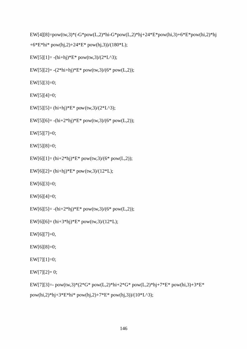
146
EW[4][8]=pow(tw,3)*(-G*pow(L,2)*hi-G*pow(L,2)*hj+24*E*pow(hi,3)+6*E*pow(hi,2)*hj
+6*E*hi* pow(hj,2)+24*E* pow(hj,3))/(180*L);
EW[5][1]= -(hi+hj)*E* pow(tw,3)/(2*L^3);
EW[5][2]= -(2*hi+hj)*E* pow(tw,3)/(6* pow(L,2));
EW[5][3]=0;
EW[5][4]=0;
EW[5][5]= (hi+hj)*E* pow(tw,3)/(2*L^3);
EW[5][6]= -(hi+2*hj)*E* pow(tw,3)/(6* pow(L,2));
EW[5][7]=0;
EW[5][8]=0;
EW[6][1]= (hi+2*hj)*E* pow(tw,3)/(6* pow(L,2));
EW[6][2]= (hi+hj)*E* pow(tw,3)/(12*L);
EW[6][3]=0;
EW[6][4]=0;
EW[6][5]= -(hi+2*hj)*E* pow(tw,3)/(6* pow(L,2));
EW[6][6]= (hi+3*hj)*E* pow(tw,3)/(12*L);
EW[6][7]=0,
EW[6][8]=0;
EW[7][1]=0;
EW[7][2]= 0;
EW[7][3]=- pow(tw,3)*(2*G* pow(L,2)*hi+2*G* pow(L,2)*hj+7*E* pow(hi,3)+3*E*
pow(hi,2)*hj+3*E*hi* pow(hj,2)+7*E* pow(hj,3))/(10*L^3);
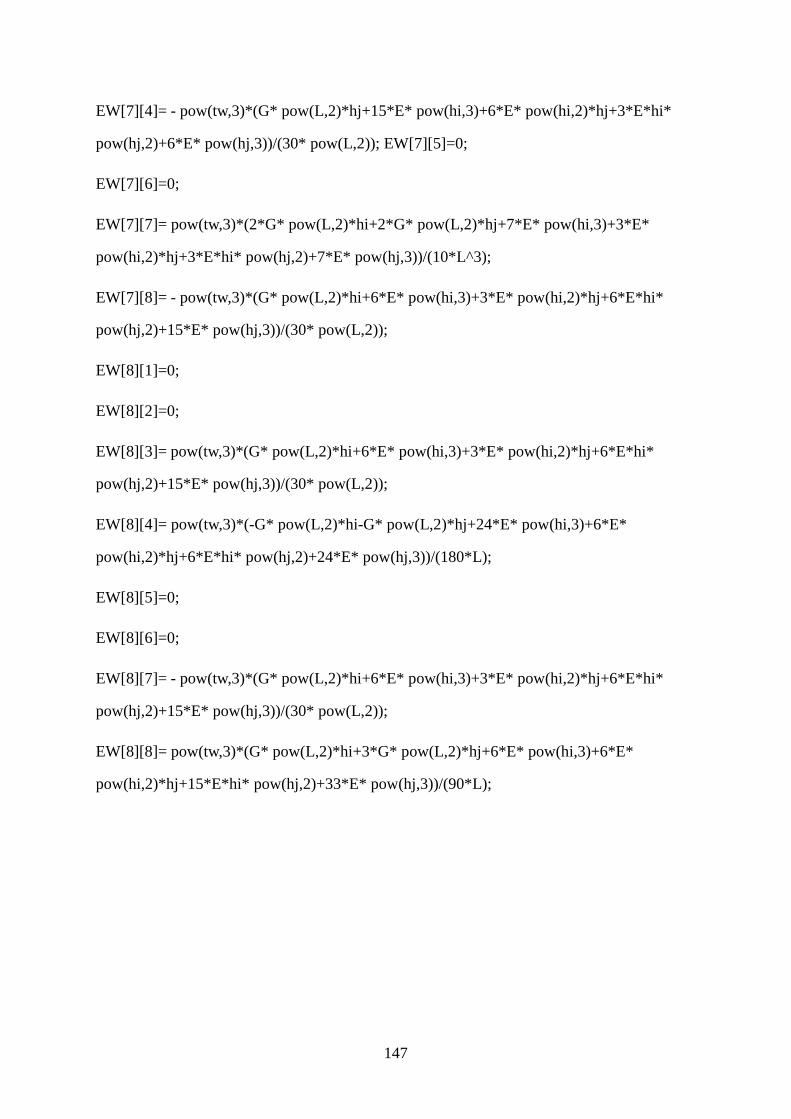
147
EW[7][4]= - pow(tw,3)*(G* pow(L,2)*hj+15*E* pow(hi,3)+6*E* pow(hi,2)*hj+3*E*hi*
pow(hj,2)+6*E* pow(hj,3))/(30* pow(L,2)); EW[7][5]=0;
EW[7][6]=0;
EW[7][7]= pow(tw,3)*(2*G* pow(L,2)*hi+2*G* pow(L,2)*hj+7*E* pow(hi,3)+3*E*
pow(hi,2)*hj+3*E*hi* pow(hj,2)+7*E* pow(hj,3))/(10*L^3);
EW[7][8]= - pow(tw,3)*(G* pow(L,2)*hi+6*E* pow(hi,3)+3*E* pow(hi,2)*hj+6*E*hi*
pow(hj,2)+15*E* pow(hj,3))/(30* pow(L,2));
EW[8][1]=0;
EW[8][2]=0;
EW[8][3]= pow(tw,3)*(G* pow(L,2)*hi+6*E* pow(hi,3)+3*E* pow(hi,2)*hj+6*E*hi*
pow(hj,2)+15*E* pow(hj,3))/(30* pow(L,2));
EW[8][4]= pow(tw,3)*(-G* pow(L,2)*hi-G* pow(L,2)*hj+24*E* pow(hi,3)+6*E*
pow(hi,2)*hj+6*E*hi* pow(hj,2)+24*E* pow(hj,3))/(180*L);
EW[8][5]=0;
EW[8][6]=0;
EW[8][7]= - pow(tw,3)*(G* pow(L,2)*hi+6*E* pow(hi,3)+3*E* pow(hi,2)*hj+6*E*hi*
pow(hj,2)+15*E* pow(hj,3))/(30* pow(L,2));
EW[8][8]= pow(tw,3)*(G* pow(L,2)*hi+3*G* pow(L,2)*hj+6*E* pow(hi,3)+6*E*
pow(hi,2)*hj+15*E*hi* pow(hj,2)+33*E* pow(hj,3))/(90*L);
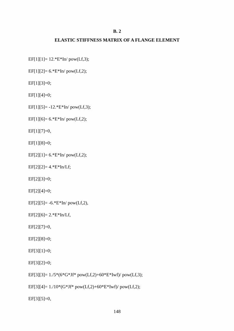
148
B. 2
ELASTIC STIFFNESS MATRIX OF A FLANGE ELEMENT
EF[1][1]= 12.*E*In/ pow(Lf,3);
EF[1][2]= 6.*E*In/ pow(Lf,2);
EF[1][3]=0;
EF[1][4]=0;
EF[1][5]= -12.*E*In/ pow(Lf,3);
EF[1][6]= 6.*E*In/ pow(Lf,2);
EF[1][7]=0,
EF[1][8]=0;
EF[2][1]= 6.*E*In/ pow(Lf,2);
EF[2][2]= 4.*E*In/Lf;
EF[2][3]=0;
EF[2][4]=0;
EF[2][5]= -6.*E*In/ pow(Lf,2),
EF[2][6]= 2.*E*In/Lf,
EF[2][7]=0,
EF[2][8]=0;
EF[3][1]=0;
EF[3][2]=0;
EF[3][3]= 1./5*(6*G*Jf* pow(Lf,2)+60*E*Iwf)/ pow(Lf,3);
EF[3][4]= 1./10*(G*Jf* pow(Lf,2)+60*E*Iwf)/ pow(Lf,2);
EF[3][5]=0,
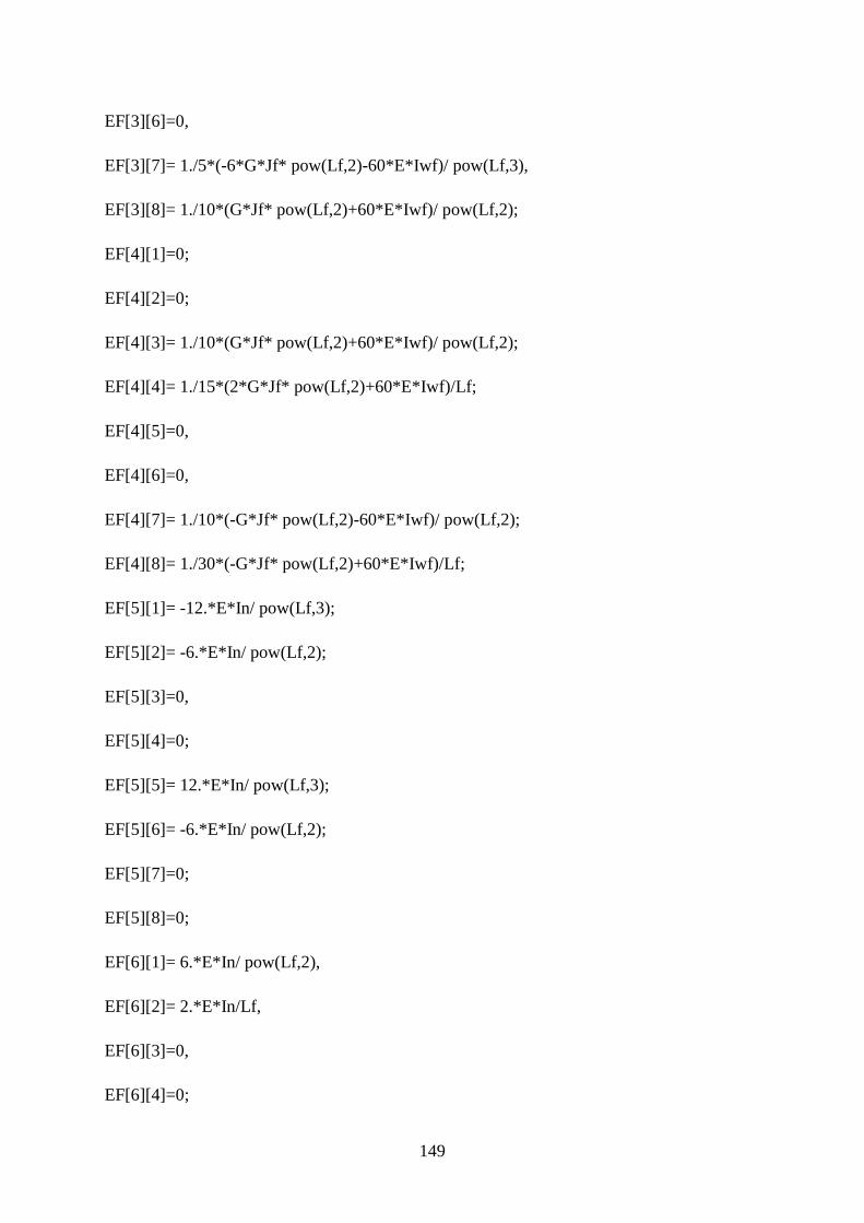
149
EF[3][6]=0,
EF[3][7]= 1./5*(-6*G*Jf* pow(Lf,2)-60*E*Iwf)/ pow(Lf,3),
EF[3][8]= 1./10*(G*Jf* pow(Lf,2)+60*E*Iwf)/ pow(Lf,2);
EF[4][1]=0;
EF[4][2]=0;
EF[4][3]= 1./10*(G*Jf* pow(Lf,2)+60*E*Iwf)/ pow(Lf,2);
EF[4][4]= 1./15*(2*G*Jf* pow(Lf,2)+60*E*Iwf)/Lf;
EF[4][5]=0,
EF[4][6]=0,
EF[4][7]= 1./10*(-G*Jf* pow(Lf,2)-60*E*Iwf)/ pow(Lf,2);
EF[4][8]= 1./30*(-G*Jf* pow(Lf,2)+60*E*Iwf)/Lf;
EF[5][1]= -12.*E*In/ pow(Lf,3);
EF[5][2]= -6.*E*In/ pow(Lf,2);
EF[5][3]=0,
EF[5][4]=0;
EF[5][5]= 12.*E*In/ pow(Lf,3);
EF[5][6]= -6.*E*In/ pow(Lf,2);
EF[5][7]=0;
EF[5][8]=0;
EF[6][1]= 6.*E*In/ pow(Lf,2),
EF[6][2]= 2.*E*In/Lf,
EF[6][3]=0,
EF[6][4]=0;
150
EF[6][5]= -6.*E*In/ pow(Lf,2);
EF[6][6]= 4.*E*In/Lf;
EF[6][7]=0;
EF[6][8]=0;
EF[7][1]=0,
EF[7][2]=0,
EF[7][3]= 1./5*(-6*G*Jf* pow(Lf,2)-60*E*Iwf)/ pow(Lf,3);
EF[7][4]= 1./10*(-G*Jf* pow(Lf,2)-60*E*Iwf)/ pow(Lf,2);
EF[7][5]=0;
EF[7][6]=0;
EF[7][7]= 1./5*(6*G*Jf* pow(Lf,2)+60*E*Iwf)/ pow(Lf,3);
EF[7][8]= 1./10*(-G*Jf* pow(Lf,2)-60*E*Iwf)/ pow(Lf,2);
EF[8][1]=0;
EF[8][2]=0;
EF[8][3]= 1./10*(G*Jf* pow(Lf,2)+60*E*Iwf)/ pow(Lf,2);
EF[8][4]= 1./30*(-G*Jf* pow(Lf,2)+60*E*Iwf)/Lf;
EF[8][5]=0;
EF[8][6]=0;
EF[8][7]= 1./10*(-G*Jf* pow(Lf,2)-60*E*Iwf)/ pow(Lf,2);
EF[8][8]= 1./15*(2*G*Jf* pow(Lf,2)+60*E*Iwf)/Lf;
151
B. 3
GEOMETRIC STIFFNESS MATRIX OF A BEAM ELEMENT
KG[1][1]=(6.*F)/(5*L);
KG[1][2]=F/10.;
KG[1][3]=(-6.*Mi)/(5*L)-Vi/10.;
KG[1][4]=-Mi/10.;
KG[1][5]=(-6.*F)/(5.*L);
KG[1][6]=F/10;
KG[1][7]=(6.*Mi)/(5.*L)+(11.*Vi)/10.;
KG[1][8]=-Mi/10.-(L*Vi)/10.;
KG[2][1]=KG[1][2];
KG[2][2]=(2.*F*L)/15.;
KG[2][3]=(-11.*Mi)/10.-(L*Vi)/5.;
KG[2][4]=-(2.*L*Mi)/15.-((L*L)*Vi)/30.;
KG[2][5]=-F/10.;
KG[2][6]=-(F*L)/30.;
KG[2][7]=Mi/10.+(L*Vi)/5.;
KG[2][8]=(L*Mi)/30.;
KG[3][1]=KG[1][3];
KG[3][2]=KG[2][3];
KG[3][3]=P*(d+h1/2+zp*0)-(6.*P*(d+h1/2+zp*0)*zp*zp)/(L*L)+(4.*P*(d+h1/2+zp*0)*zp*
zp*zp)/(L*L*L)+(9.*P*(d+h1/2+zp*0)*zp*zp*zp*zp)/(L*L*L*L)-(12.*P*(d+h1/2.+zp*0)*z
p*zp*zp*zp*zp)/(L*L*L*L*L)+(4.*P*(d+h1/2+zp*0)*zp*zp*zp*zp*zp*zp)/(L*L*L*L*L*L
);
KG[3][4]=P*(d+h1/2+zp*0)*zp-(2.*P*(d+h1/2+zp*0)*zp*zp)/L-(2.*P*(d+h1/2+zp*0)*zp*z
p*zp)/(L*L)+(8.*P*(d+h1/2+zp*0)*zp*zp*zp*zp)/(L*L*L)-(7.*P*(d+h1/2.+zp*0)*zp*zp*z
p*zp*zp)/(L*L*L*L)+(2.*P*(d+h1/2+zp*0)*zp*zp*zp*zp*zp*zp)/(L*L*L*L*L);
KG[3][5]=(6.*Mi)/(5.*L)+Vi/10.;

152
KG[3][6]=-Mi/10.+(L*Vi)/10.;
KG[3][7]=(3.*P*(d+h1/2+zp*0)*zp*zp)/(L*L)-(2.*P*(d+h1/2+zp*0)*zp*zp*zp)/(L*L*L)-(9
.*P*(d+h1/2+zp*0)*zp*zp*zp*zp)/(L*L*L*L)+(12.*P*(d+h1/2+zp*0)*zp*zp*zp*zp*zp)/(L
*L*L*L*L)-(4.*P*(d+h1/2+zp*0)*zp*zp*zp*zp*zp*zp)/(L*L*L*L*L*L);
KG[3][8]=-(P*(d+h1/2+zp*0)*zp*zp)/L+(P*(d+h1/2+zp*0)*zp*zp*zp)/(L*L)+(3.*P*(d+h1/
2+zp*0)*zp*zp*zp*zp)/(L*L*L)-(5.*P*(d+h1/2.+zp*0)*zp*zp*zp*zp*zp)/(L*L*L*L)+(2.*P
*(d+h1/2+zp*0)*zp*zp*zp*zp*zp*zp)/(L*L*L*L*L);
KG[4][1]=KG[1][4];
KG[4][2]=KG[2][4];
KG[4][3]=KG[3][4];
KG[4][4]=P*(d+h1/2+zp*0)*zp*zp-(4.*P*(d+h1/2.+zp*0)*zp*zp*zp)/L+(6.*P*(d+h1/2.+zp
*0)*zp*zp*zp*zp)/(L*L)-(4.*P*(d+h1/2.+zp*0)*zp*zp*zp*zp*zp)/(L*L*L)+(P*(d+h1/2.+zp
*0)*zp*zp*zp*zp*zp*zp)/(L*L*L*L);
KG[4][5]=Mi/10;
KG[4][6]=(L*Mi)/30.+((L*L)*Vi)/30;
KG[4][7]=(3.*P*(d+h1/2+zp*0)*zp*zp*zp)/(L*L)-(8.*P*(d+h1/2+zp*0)*zp*zp*zp*zp)/(L*
L*L)+(7.*P*(d+h1/2.+zp*0)*zp*zp*zp*zp*zp)/(L*L*L*L)-(2.*P*(d+h1/2.+zp*0)*zp*zp*zp
*zp*zp*zp)/(L*L*L*L*L);
KG[4][8]=-(P*(d+h1/2+zp*0)*zp*zp*zp)/L+(3.*P*(d+h1/2+zp*0)*zp*zp*zp*zp)/(L*L)-(3.*
P*(d+h1/2+zp*0)*zp*zp*zp*zp*zp)/(L*L*L)+(P*(d+h1/2+zp*0)*zp*zp*zp*zp*zp*zp)/(L*
L*L*L);
KG[5][1]=KG[1][5];
KG[5][2]=KG[2][5];
KG[5][3]=KG[3][5];
KG[5][4]=KG[4][5];
KG[5][5]=(6.*F)/(5.*L);
KG[5][6]=-F/10.;
KG[5][7]=(-6.*Mi)/(5.*L)-(11.*Vi)/10.;
153
KG[5][8]=Mi/10.+(L*Vi)/10.;
KG[6][1]=KG[1][6];
KG[6][2]=KG[2][6];
KG[6][3]=KG[3][6];
KG[6][4]=KG[4][6];
KG[6][5]=KG[5][6];
KG[6][6]=(2.*F*L)/15;
KG[6][7]=(11.*Mi)/10+(9.*L*Vi)/10;
KG[6][8]=(-2.*L*Mi)/15-((L*L)*Vi)/10.;
KG[7][1]=KG[1][7];
KG[7][2]=KG[2][7];
KG[7][3]=KG[3][7];
KG[7][4]=KG[4][7];
KG[7][5]=KG[5][7];
KG[7][6]=KG[6][7];
KG[7][7]=(9.*P*(d+h1/2+zp*0)*zp*zp*zp*zp)/(L*L*L*L)-(12.*P*(d+h1/2+zp*0)*zp*zp*z
p*zp*zp)/(L*L*L*L*L)+(4.*P*(d+h1/2+zp*0)*zp*zp*zp*zp*zp*zp)/(L*L*L*L*L*L);
KG[7][8]=-(3.*P*(d+h1/2+zp*0)*zp*zp*zp*zp)/(L*L*L)+(5.*P*(d+h1/2+zp*0)*zp*zp*zp*
zp*zp)/(L*L*L*L)-(2.*P*(d+h1/2+zp*0)*zp*zp*zp*zp*zp*zp)/(L*L*L*L*L);
KG[8][1]=KG[1][8];
KG[8][2]=KG[2][8];
KG[8][3]=KG[3][8];
KG[8][4]=KG[4][8];
KG[8][5]=KG[5][8];
KG[8][6]=KG[6][8];
KG[8][7]=KG[7][8];
KG[8][8]=(P*(d+h1/2)*zp*zp*zp*zp)/(L*L)-(2.*P*(d+h1/2+zp*0)*zp*zp*zp*zp*zp)/(L*L*
L)+(P*(d+h1/2+zp*0)*zp*zp*zp*zp*zp*zp)/(L*L*L*L);
154
APPENDIX C
FLEXURAL-TORSIONAL BUCKLING ANALYSIS PROGRAM
This Appendix presents the code written for the LBuck Program.
C.1 PROP.H
#if!defined(properties_h) #define propereties_h #define MSize 62 class Properties protected: int j1,j2,joint_num; float E,G,Jf,Iwf,L,Lf,In,tw,d,zi,zj,hi,hj,tanA0,A0,element_num,length; float Fi,Vi,Vj,Mi; float z[MSize]; float h[MSize]; float v[MSize]; float mi[MSize]; public: virtual void Fill_Properties(int, int, float)=0; ;
#endif
155
C.2 ELEMENTSTIFF.H
#if!defined(element_stiffness_h) #define element_stiffness_h #define MSize 62 class Element_Stiffness:public Properties /* Inheritance */ private: float KE[MSize][MSize]; float EW[MSize][MSize]; float EF[MSize][MSize]; float P[MSize][MSize]; float Q[MSize][MSize]; float PT[MSize][MSize]; float QT[MSize][MSize]; float C[MSize][MSize]; float CT[MSize][MSize]; float DT[MSize][MSize]; float D[MSize][MSize]; float X1[MSize][MSize]; float X2[MSize][MSize]; float X3[MSize][MSize]; float X4[MSize][MSize]; float Y1[MSize][MSize]; float Y2[MSize][MSize]; float Y3[MSize][MSize]; float Y4[MSize][MSize]; public: friend int main(); friend class Stiffness; void Fill_Element_Stiffness(float, int, float); void Fill_Properties(int, int, float); ; #endif
156
C.3 ELEMENTGEOM.H
#if!defined(element_geometric_h) #define element_geometric_h #define MSize 62 class Element_Geometric:public Properties private: float KG[MSize][MSize]; float GW[MSize][MSize]; float GF[MSize][MSize]; float P[MSize][MSize]; float Q[MSize][MSize]; float PT[MSize][MSize]; float QT[MSize][MSize]; float C[MSize][MSize]; float CT[MSize][MSize]; float DT[MSize][MSize]; float D[MSize][MSize]; float X1[MSize][MSize]; float X2[MSize][MSize]; float X3[MSize][MSize]; float X4[MSize][MSize]; float Y1[MSize][MSize]; float Y2[MSize][MSize]; float Y3[MSize][MSize]; float Y4[MSize][MSize]; public: friend class Geometric; void Fill_Element_Geometric(float,int,float); void Fill_Properties(int, int, float); ; #endif
157
C.4 STIFFN.H
#if!defined(stiffness_h) #define stiffness_h #define MSize 62 class Stiffness private: Element_Stiffness stiff; //Element Stiffness matrix int element_num;//number of elements float length; public: float A[MSize][MSize]; Stiffness(int); void Assembling_Stiffness_Matrix(float,int,float); ; #endif
C.5 GEOMTR.H
#if!defined(geometric_h) #define geometric_h #define MSize 62 class Geometric private: Element_Geometric geom; //element geometric matrix int element_num; //number of elements float length; public: float B[MSize][MSize]; Geometric(int); void Assembling_Geometric_Matrix(float,int,float); ; #endif
158
C.6 SPPRT.H
#if!defined(support_h) #define support_h #define MSize 62 class Supports private: int restrain[MSize]; int rest; int size; //Total degrees of freedom int free_size; //Free degrees of freedom public: Supports(int); void Get_boundary_conditions(); int Boundary_Condition(float[MSize][MSize],float[MSize][MSize]); ; #endif
C.7 STANDM.H
#if!defined(standard_matrix_h) #define standard_matrix_h #define MSize 62 class Standard_Matrix private: int size; float dia[MSize]; float C[MSize][MSize]; float off[MSize]; float buckling_load; public: Standard_Matrix(); void standard_matrix(float[MSize][MSize],float[MSize][MSize],int); float pythag(float,float);
159
void choldc(float[MSize][MSize]); void tred2(float[MSize][MSize]); void tqli(float[MSize][MSize]); float getBucklingLoad(); ; #endif
C.8 PROP. CPP
#include<iostream> #include<fstream> #include<stdio.h> #include"math.h" #include"prop.h" using namespace std; //Fill Element Properties void Properties::Fill_Properties(int j, int element_num, float length) double PI=3.14159265; joint_num=element_num+1; float P=0.; float L=length/element_num; //in float A0=0.0; for(int i=1;i<MSize;i++) z[i]=0.0;h[i]=0.;v[i]=0.;mi[i]=0.0; for(int i=1;i<=joint_num;i++) z[i]=(i-1)*L; zi=z[j]; zj=z[j+1]; for(int i=2;i<=joint_num;i++) h[1]=13.12; h[i]=h[i-1]+2*L*tan(A0); cout<<h[i]<<endl; hi=h[j]; hj=h[j+1]; for(int i=1;i<=joint_num;i++) v[i]=P; v[joint_num]=0.;
160
Vi=v[j]; Vj=v[j+1]; for(int i=1;i<=joint_num;i++) mi[i]=10000;
Mi=mi[j];
C.9 ELEMENTSTIFF. CPP
#include<iostream> #include<fstream> #include<stdio.h> #include"math.h" #include"prop.h" #include"elementstiff.h" using namespace std; static double PI=3.14159265; void Element_Stiffness::Fill_Properties(int j,int element_num,float length) Properties::Fill_Properties(j,element_num,length); void Element_Stiffness::Fill_Element_Stiffness(float K, int element_num,float length) ofstream SaveFile("KE.txt"); float E=30000; //ksi float G=12000; //ksi float Jf=5.54; //in^4 float tw=0.71; //in float tf=1.105; //in float In=172.19; //in^4 float Iwf;//in^6 Iwf=In*pow((hi+hj-2*tf)/2,2)/4; cout<<"Iwf="<<Iwf<<endl; float L=length/element_num; //in
161
float A0=-0.0; //rad float Lf=L/cos(A0); for(int i=1;i<MSize;i++) for(int j=1;j<MSize;j++)
EW[i][j]=0.;EF[i][j]=0;C[i][j]=0;CT[i][j]=0;D[i][j]=0;DT[i][j]=0;P[i][j]=0; PT[i][j]=0;Q[i][j]=0;QT[i][j]=0;KE[i][j]=0;X1[i][j]=0;X2[i][j]=0;X3[i][j]=0; X4[i][j]=0; Y1[i][j]=0;Y2[i][j]=0;Y3[i][j]=0;Y4[i][j]=0;
EW[1][1]=1./2*(hi+hj)*E*pow(tw,3)/pow(L,3); EW[1][2]=1./6*(2*hi+hj)*E*pow(tw,3)/pow(L,2); EW[1][3]=0; EW[1][4]=0; EW[1][5]=1./2*(-hi-hj)*E*pow(tw,3)/pow(L,3); EW[1][6]=1./6*(hi+2*hj)*E*pow(tw,3)/pow(L,2); EW[1][7]=0; EW[1][8]=0; EW[2][1]=1./6*(2*hi+hj)*E*pow(tw,3)/pow(L,2); EW[2][2]=1./12*(3*hi+hj)*E*pow(tw,3)/L; EW[2][3]=0; EW[2][4]=0; EW[2][5]=1./6*(-2*hi-hj)*E*pow(tw,3)/ pow(L,2); EW[2][6]=1./12*(hi+hj)*E*pow(tw,3)/L; EW[2][7]=0; EW[2][8]=0; EW[3][1]=0; EW[3][2]=0; EW[3][3]=pow(tw,3)*(2*G*pow(L,2)*hi+2*G*pow(L,2)*hj+7*E*pow(hi,3)+3*E*pow(hi,2)*hj+3*E*hi*pow(hj,2)+7*E*pow(hj,3))/(10* pow(L,3)); EW[3][4]=pow(tw,3)*(G*pow(L,2)*hj+15*E*pow(hi,3)+6*E*pow(hi,2)*hj+3*E*hi*pow(hj,2)+6*E*pow(hj,3))/(30*pow(L,2)); EW[3][5]=0; EW[3][6]=0; EW[3][7]=-pow(tw,3)*(2*G*pow(L,2)*hi+2*G*pow(L,2)*hj+7*E*pow(hi,3)+3*E*pow(hi,2)*hj+3*E*hi*pow(hj,2)+7*E*pow(hj,3))/(10*pow(L,3)); EW[3][8]=pow(tw,3)*(G*pow(L,2)*hi+6*E*pow(hi,3)+3*E*pow(hi,2)*hj+6*E*hi*pow(hj,2)+15*E*pow(hj,3))/(30*pow(L,2)); EW[4][1]=0; EW[4][2]=0; EW[4][3]=pow(tw,3)*(G*pow(L,2)*hj+15*E*pow(hi,3)+6*E*pow(hi,2)*hj+3*E*hi*pow(hj,2)+6*E*pow(hj,3))/(30*pow(L,2)); EW[4][4]=pow(tw,3)*(3*G*pow(L,2)*hi+G*pow(L,2)*hj+33*E*pow(hi,3)+15*E*pow(hi,2)*hj+6*E*hi*pow(hj,2)+6*E*pow(hj,3))/(90*L);
162
EW[4][5]=0; EW[4][6]=0; EW[4][7]=-pow(tw,3)*(G*pow(L,2)*hj+15*E*pow(hi,3)+6*E*pow(hi,2)*hj+3*E*hi*pow(hj,2)+6*E*pow(hj,3))/(30*pow(L,2)); EW[4][8]=pow(tw,3)*(-G*pow(L,2)*hi-G*pow(L,2)*hj+24*E*pow(hi,3)+6*E*pow(hi,2)*hj+6*E*hi*pow(hj,2)+24*E*pow(hj,3))/(180*L); EW[5][1]=-(hi+hj)*E*pow(tw,3)/(2*pow(L,3)); EW[5][2]=-(2*hi+hj)*E*pow(tw,3)/(6*pow(L,2)); EW[5][3]=0; EW[5][4]=0; EW[5][5]=(hi+hj)*E*pow(tw,3)/(2*pow(L,3)); EW[5][6]=-(hi+2*hj)*E*pow(tw,3)/(6*pow(L,2)); EW[5][7]=0; EW[5][8]=0; EW[6][1]=(hi+2*hj)*E*pow(tw,3)/(6*pow(L,2)); EW[6][2]=(hi+hj)*E*pow(tw,3)/(12*L); EW[6][3]=0; EW[6][4]=0; EW[6][5]=-(hi+2*hj)*E*pow(tw,3)/(6*pow(L,2)); EW[6][6]=(hi+3*hj)*E*pow(tw,3)/(12*L); EW[6][7]=0; EW[6][8]=0; EW[7][1]=0; EW[7][2]=0; EW[7][3]=-pow(tw,3)*(2*G*pow(L,2)*hi+2*G*pow(L,2)*hj+7*E*pow(hi,3)+3*E*pow(hi,2)*hj+3*E*hi*pow(hj,2)+7*E*pow(hj,3))/(10*pow(L,3)); EW[7][4]=-pow(tw,3)*(G*pow(L,2)*hj+15*E*pow(hi,3)+6*E*pow(hi,2)*hj+3*E*hi*pow(hj,2)+6*E*pow(hj,3))/(30*pow(L,2)); EW[7][5]=0; EW[7][6]=0; EW[7][7]=pow(tw,3)*(2*G*pow(L,2)*hi+2*G*pow(L,2)*hj+7*E*pow(hi,3)+3*E*pow(hi,2)*hj+3*E*hi*pow(hj,2)+7*E*pow(hj,3))/(10*pow(L,3)); EW[7][8]=-pow(tw,3)*(G*pow(L,2)*hi+6*E*pow(hi,3)+3*E*pow(hi,2)*hj+6*E*hi*pow(hj,2)+15*E*pow(hj,3))/(30*pow(L,2)); EW[8][1]=0; EW[8][2]=0; EW[8][3]=pow(tw,3)*(G*pow(L,2)*hi+6*E*pow(hi,3)+3*E*pow(hi,2)*hj+6*E*hi*pow(hj,2)+15*E*pow(hj,3))/(30*pow(L,2)); EW[8][4]=pow(tw,3)*(-G*pow(L,2)*hi-G*pow(L,2)*hj+24*E*pow(hi,3)+6*E*pow(hi,2)*hj+6*E*hi*pow(hj,2)+24*E*pow(hj,3))/(180*L); EW[8][5]=0; EW[8][6]=0;
163
EW[8][7]=-pow(tw,3)*(G*pow(L,2)*hi+6*E*pow(hi,3)+3*E*pow(hi,2)*hj+6*E*hi*pow(hj,2)+15*E*pow(hj,3))/(30*pow(L,2)); EW[8][8]=pow(tw,3)*(G*pow(L,2)*hi+3*G*pow(L,2)*hj+6*E*pow(hi,3)+6*E*pow(hi,2)*hj+15*E*hi*pow(hj,2)+33*E*pow(hj,3))/(90*L); EF[1][1]=12.*E*In/pow(Lf,3); EF[1][2]=6.*E*In/pow(Lf,2); EF[1][3]=0; EF[1][4]=0; EF[1][5]=-12.*E*In/pow(Lf,3); EF[1][6]=6.*E*In/pow(Lf,2); EF[1][7]=0; EF[1][8]=0; EF[2][1]=6.*E*In/pow(Lf,2); EF[2][2]=4.*E*In/Lf; EF[2][3]=0; EF[2][4]=0; EF[2][5]=-6.*E*In/pow(Lf,2); EF[2][6]=2.*E*In/Lf; EF[2][7]=0; EF[2][8]=0; EF[3][1]=0; EF[3][2]=0; EF[3][3]=1./5*(6*G*Jf*pow(Lf,2)+60*E*Iwf)/pow(Lf,3); EF[3][4]=1./10*(G*Jf*pow(Lf,2)+60*E*Iwf)/pow(Lf,2); EF[3][5]=0; EF[3][6]=0; EF[3][7]=1./5*(-6*G*Jf*pow(Lf,2)-60*E*Iwf)/pow(Lf,3); EF[3][8]=1./10*(G*Jf*pow(Lf,2)+60*E*Iwf)/pow(Lf,2); EF[4][1]=0; EF[4][2]=0; EF[4][3]=1./10*(G*Jf*pow(Lf,2)+60*E*Iwf)/pow(Lf,2); EF[4][4]=1./15*(2*G*Jf*pow(Lf,2)+60*E*Iwf)/Lf; EF[4][5]=0; EF[4][6]=0; EF[4][7]=1./10*(-G*Jf*pow(Lf,2)-60*E*Iwf)/pow(Lf,2); EF[4][8]=1./30*(-G*Jf*pow(Lf,2)+60*E*Iwf)/Lf; EF[5][1]=-12.*E*In/pow(Lf,3); EF[5][2]=-6.*E*In/pow(Lf,2); EF[5][3]=0; EF[5][4]=0; EF[5][5]=12.*E*In/pow(Lf,3);
164
EF[5][6]=-6.*E*In/pow(Lf,2); EF[5][7]=0; EF[5][8]=0; EF[6][1]=6.*E*In/pow(Lf,2); EF[6][2]=2.*E*In/Lf; EF[6][3]=0; EF[6][4]=0; EF[6][5]=-6.*E*In/pow(Lf,2); EF[6][6]=4.*E*In/Lf; EF[6][7]=0; EF[6][8]=0; EF[7][1]=0; EF[7][2]=0; EF[7][3]=1./5*(-6*G*Jf*pow(Lf,2)-60*E*Iwf)/pow(Lf,3); EF[7][4]=1./10*(-G*Jf*pow(Lf,2)-60*E*Iwf)/pow(Lf,2); EF[7][5]=0; EF[7][6]=0; EF[7][7]=1./5*(6*G*Jf*pow(Lf,2)+60*E*Iwf)/pow(Lf,3); EF[7][8]=1./10*(-G*Jf*pow(Lf,2)-60*E*Iwf)/pow(Lf,2); EF[8][1]=0; EF[8][2]=0; EF[8][3]=1./10*(G*Jf*pow(Lf,2)+60*E*Iwf)/pow(Lf,2); EF[8][4]=1./30*(-G*Jf*pow(Lf,2)+60*E*Iwf)/Lf; EF[8][5]=0; EF[8][6]=0; EF[8][7]=1./10*(-G*Jf*pow(Lf,2)-60*E*Iwf)/pow(Lf,2); EF[8][8]=1./15*(2*G*Jf*pow(Lf,2)+60*E*Iwf)/Lf; Q[1][1]=1; Q[2][2]=1; Q[3][3]=1; Q[4][4]=1; Q[5][5]=1; Q[6][6]=1; Q[7][7]=1; Q[8][8]=1; /*Q[1][3]=hi/2; Q[2][3]=tan(A0); Q[2][4]=hi/2; Q[5][7]=hj/2; Q[6][7]=tan(A0); Q[6][8]=hj/2;*/
165
QT[1][1]=1; QT[2][2]=1; QT[3][3]=1; QT[4][4]=1; QT[5][5]=1; QT[6][6]=1; QT[7][7]=1; QT[8][8]=1; /*QT[3][1]=hi/2; QT[3][2]=tan(A0); QT[4][2]=hi/2; QT[7][5]=hj/2; QT[7][6]=tan(A0); QT[8][6]=hj/2;*/ P[1][1]=1; P[2][2]=cos(A0); P[3][3]=cos(A0); P[4][4]=1; P[5][5]=1; P[6][6]=cos(A0); P[7][7]=cos(A0); P[8][8]=1; P[2][3]=sin(A0); P[3][2]=-sin(A0); P[6][7]=sin(A0); P[7][6]=-sin(A0); PT[1][1]=1; PT[2][2]=cos(A0); PT[3][3]=cos(A0); PT[4][4]=1; PT[5][5]=1; PT[6][6]=cos(A0); PT[7][7]=cos(A0); PT[8][8]=1; PT[3][2]=sin(A0); PT[2][3]=-sin(A0); PT[7][6]=sin(A0); PT[6][7]=-sin(A0);
166
C[1][1]=1; C[2][2]=cos(A0); C[3][3]=cos(A0); C[4][4]=1; C[5][5]=1; C[6][6]=cos(A0); C[7][7]=cos(A0); C[8][8]=1; C[2][3]=-sin(A0); C[3][2]=sin(A0); C[6][7]=-sin(A0); C[7][6]=sin(A0); CT[1][1]=1; CT[2][2]=cos(A0); CT[3][3]=cos(A0); CT[4][4]=1; CT[5][5]=1; CT[6][6]=cos(A0); CT[7][7]=cos(A0); CT[8][8]=1; CT[3][2]=-sin(A0); CT[2][3]=sin(A0); CT[7][6]=-sin(A0); CT[6][7]=sin(A0); D[1][1]=1; D[2][2]=1; D[3][3]=1; D[4][4]=1; D[5][5]=1; D[6][6]=1; D[7][7]=1; D[8][8]=1; /*D[1][3]=-hi/2; D[2][3]=-tan(A0); D[2][4]=-hi/2; D[5][7]=-hj/2; D[6][7]=-tan(A0); D[6][8]=-hj/2;*/
167
DT[1][1]=1; DT[2][2]=1; DT[3][3]=1; DT[4][4]=1; DT[5][5]=1; DT[6][6]=1; DT[7][7]=1; DT[8][8]=1; /*DT[3][1]=-hi/2; DT[3][2]=-tan(A0); DT[4][2]=-hi/2; DT[7][5]=-hj/2; DT[7][6]=-tan(A0); DT[8][6]=-hj/2;*/ for(int i=1;i<=8;i++) for(int j=1;j<=8;j++) for(int k=1;k<=8;k++) X1[i][j]=X1[i][j]+QT[i][k]*PT[k][j]; for(int i=1;i<=8;i++) for(int j=1;j<=8;j++) for(int k=1;k<=8;k++) X2[i][j]=X2[i][j]+X1[i][k]*EF[k][j]; for(int i=1;i<=8;i++) for(int j=1;j<=8;j++) for(int k=1;k<=8;k++) X3[i][j]=X3[i][j]+X2[i][k]*P[k][j]; for(int i=1;i<=8;i++) for(int j=1;j<=8;j++) for(int k=1;k<=8;k++) X4[i][j]=X4[i][j]+X3[i][k]*Q[k][j]; for(int i=1;i<=8;i++) for(int j=1;j<=8;j++) for(int k=1;k<=8;k++) Y1[i][j]=Y1[i][j]+DT[i][k]*CT[k][j];
168
for(int i=1;i<=8;i++) for(int j=1;j<=8;j++) for(int k=1;k<=8;k++) Y2[i][j]=Y2[i][j]+Y1[i][k]*EF[k][j]; for(int i=1;i<=8;i++) for(int j=1;j<=8;j++) for(int k=1;k<=8;k++) Y3[i][j]=Y3[i][j]+Y2[i][k]*C[k][j]; for(int i=1;i<=8;i++) for(int j=1;j<=8;j++) for(int k=1;k<=8;k++) Y4[i][j]=Y4[i][j]+Y3[i][k]*D[k][j]; for(int i=1;i<=8;i++) for(int j=1;j<=8;j++) KE[i][j]=EW[i][j]+X4[i][j]+Y4[i][j]; for(int j=1;j<=8;j++) for(int k=1;k<=8;k++) SaveFile<<"KE["<<j<<"]["<<k<<"]="<<KE[j][k]<<endl; SaveFile.close();
C.10 ELEMENTGEOM. CPP
#include<iostream> #include<fstream> #include<stdio.h> #include"math.h" #include"prop.h" #include"elementgeom.h" using namespace std; static double PI=3.14159265; void Element_Geometric::Fill_Properties(int j,int element_num,float length)
169
Properties::Fill_Properties(j,element_num,length); /* n means the number of elements*/ void Element_Geometric::Fill_Element_Geometric(float n,int element_num,float length) ofstream SaveFile("KG.txt"); int i=0; float L=length/element_num; //in float A0=-0.0; //rad float h1=13.12; //inch float d=-h1/2; //in distance of the loading above the flange float zp=length; float q=0.; float P=0.; //kips float F=0.; for(int i=1;i<MSize;i++) for(int j=1;j<MSize;j++) KG[i][j]=0; KG[1][1]=(6.*F)/(5*L); KG[1][2]=F/10.; KG[1][3]=(-6.*Mi)/(5*L)-Vi/10.; KG[1][4]=-Mi/10.; KG[1][5]=(-6.*F)/(5.*L); KG[1][6]=F/10; KG[1][7]=(6.*Mi)/(5.*L)+(11.*Vi)/10.; KG[1][8]=-Mi/10.-(L*Vi)/10.; KG[2][1]=KG[1][2]; KG[2][2]=(2.*F*L)/15.; KG[2][3]=(-11.*Mi)/10.-(L*Vi)/5.; KG[2][4]=-(2.*L*Mi)/15.-((L*L)*Vi)/30.; KG[2][5]=-F/10.; KG[2][6]=-(F*L)/30.; KG[2][7]=Mi/10.+(L*Vi)/5.; KG[2][8]=(L*Mi)/30.; KG[3][1]=KG[1][3]; KG[3][2]=KG[2][3]; KG[3][3]=P*(d+h1/2+zp*0)-(6.*P*(d+h1/2+zp*0)*zp*zp)/(L*L)+(4.*P*(d+h1/2+zp*0)*zp*zp*zp)/(L*L*L)+(9.*P*(d+h1/2+zp*0)*zp*zp*zp*zp)/(L*L*L*L)-(12.*P*(d+h1/2.+zp*0)*zp*zp*zp*zp*zp)/(L*L*L*L*L)+(4.*P*(d+h1/2+zp*0)*zp*zp*zp*zp*zp*zp)/(L*L*L*L*L*L);
170
KG[3][4]=P*(d+h1/2+zp*0)*zp-(2.*P*(d+h1/2+zp*0)*zp*zp)/L-(2.*P*(d+h1/2+zp*0)*zp*zp*zp)/(L*L)+(8.*P*(d+h1/2+zp*0)*zp*zp*zp*zp)/(L*L*L)-(7.*P*(d+h1/2.+zp*0)*zp*zp*zp*zp*zp)/(L*L*L*L)+(2.*P*(d+h1/2+zp*0)*zp*zp*zp*zp*zp*zp)/(L*L*L*L*L); KG[3][5]=(6.*Mi)/(5.*L)+Vi/10.; KG[3][6]=-Mi/10.+(L*Vi)/10.; KG[3][7]=(3.*P*(d+h1/2+zp*0)*zp*zp)/(L*L)-(2.*P*(d+h1/2+zp*0)*zp*zp*zp)/(L*L*L)-(9.*P*(d+h1/2+zp*0)*zp*zp*zp*zp)/(L*L*L*L)+(12.*P*(d+h1/2+zp*0)*zp*zp*zp*zp*zp)/(L*L*L*L*L)-(4.*P*(d+h1/2+zp*0)*zp*zp*zp*zp*zp*zp)/(L*L*L*L*L*L); KG[3][8]=-(P*(d+h1/2+zp*0)*zp*zp)/L+(P*(d+h1/2+zp*0)*zp*zp*zp)/(L*L)+(3.*P*(d+h1/2+zp*0)*zp*zp*zp*zp)/(L*L*L)-(5.*P*(d+h1/2.+zp*0)*zp*zp*zp*zp*zp)/(L*L*L*L)+(2.*P*(d+h1/2+zp*0)*zp*zp*zp*zp*zp*zp)/(L*L*L*L*L); KG[4][1]=KG[1][4]; KG[4][2]=KG[2][4]; KG[4][3]=KG[3][4]; KG[4][4]=P*(d+h1/2+zp*0)*zp*zp-(4.*P*(d+h1/2.+zp*0)*zp*zp*zp)/L+(6.*P*(d+h1/2.+zp*0)*zp*zp*zp*zp)/(L*L)-(4.*P*(d+h1/2.+zp*0)*zp*zp*zp*zp*zp)/(L*L*L)+(P*(d+h1/2.+zp*0)*zp*zp*zp*zp*zp*zp)/(L*L*L*L); KG[4][5]=Mi/10; KG[4][6]=(L*Mi)/30.+((L*L)*Vi)/30; KG[4][7]=(3.*P*(d+h1/2+zp*0)*zp*zp*zp)/(L*L)-(8.*P*(d+h1/2+zp*0)*zp*zp*zp*zp)/(L*L*L)+(7.*P*(d+h1/2.+zp*0)*zp*zp*zp*zp*zp)/(L*L*L*L)-(2.*P*(d+h1/2.+zp*0)*zp*zp*zp*zp*zp*zp)/(L*L*L*L*L); KG[4][8]=-(P*(d+h1/2+zp*0)*zp*zp*zp)/L+(3.*P*(d+h1/2+zp*0)*zp*zp*zp*zp)/(L*L)-(3.*P*(d+h1/2+zp*0)*zp*zp*zp*zp*zp)/(L*L*L)+(P*(d+h1/2+zp*0)*zp*zp*zp*zp*zp*zp)/(L*L*L*L); KG[5][1]=KG[1][5]; KG[5][2]=KG[2][5]; KG[5][3]=KG[3][5]; KG[5][4]=KG[4][5]; KG[5][5]=(6.*F)/(5.*L); KG[5][6]=-F/10.; KG[5][7]=(-6.*Mi)/(5.*L)-(11.*Vi)/10.; KG[5][8]=Mi/10.+(L*Vi)/10.; KG[6][1]=KG[1][6]; KG[6][2]=KG[2][6]; KG[6][3]=KG[3][6]; KG[6][4]=KG[4][6]; KG[6][5]=KG[5][6]; KG[6][6]=(2.*F*L)/15; KG[6][7]=(11.*Mi)/10+(9.*L*Vi)/10; KG[6][8]=(-2.*L*Mi)/15-((L*L)*Vi)/10.;
171
KG[7][1]=KG[1][7]; KG[7][2]=KG[2][7]; KG[7][3]=KG[3][7]; KG[7][4]=KG[4][7]; KG[7][5]=KG[5][7]; KG[7][6]=KG[6][7]; KG[7][7]=(9.*P*(d+h1/2+zp*0)*zp*zp*zp*zp)/(L*L*L*L)-(12.*P*(d+h1/2+zp*0)*zp*zp*zp*zp*zp)/(L*L*L*L*L)+(4.*P*(d+h1/2+zp*0)*zp*zp*zp*zp*zp*zp)/(L*L*L*L*L*L); KG[7][8]=-(3.*P*(d+h1/2+zp*0)*zp*zp*zp*zp)/(L*L*L)+(5.*P*(d+h1/2+zp*0)*zp*zp*zp*zp*zp)/(L*L*L*L)-(2.*P*(d+h1/2+zp*0)*zp*zp*zp*zp*zp*zp)/(L*L*L*L*L); KG[8][1]=KG[1][8]; KG[8][2]=KG[2][8]; KG[8][3]=KG[3][8]; KG[8][4]=KG[4][8]; KG[8][5]=KG[5][8]; KG[8][6]=KG[6][8]; KG[8][7]=KG[7][8]; KG[8][8]=(P*(d+h1/2)*zp*zp*zp*zp)/(L*L)-(2.*P*(d+h1/2+zp*0)*zp*zp*zp*zp*zp)/(L*L*L)+(P*(d+h1/2+zp*0)*zp*zp*zp*zp*zp*zp)/(L*L*L*L); for(int j=1;j<=8;j++) for(int k=1;k<=8;k++) SaveFile<<"KG["<<j<<"]["<<k<<"]="<<KG[j][k]<<endl; SaveFile.close();
C.11 STIFFN. CPP
#include "prop.h" #include "elementstiff.h" #include "stiffn.h" #include<iostream> using namespace std; //Constructor Stiffness::Stiffness(int e) for(int i=1;i<MSize;i++)
172
for(int j=1;j<MSize;j++) A[i][j]=0.0; element_num=e; //Assemble element stiffness matrices,KE, //to a structural stiffness matrix, A void Stiffness::Assembling_Stiffness_Matrix(float K, int element_num,float length) int j1=1;int j2=2; for(int i=1;i<=element_num;i++) //for each element stiff.Fill_Properties(i,element_num,length);//Read in properties //Fill element matrix; stiff.Fill_Element_Stiffness(K,element_num,length); for(int j=1;j<=4;j++) //Fill Global Matrix for(int k=1;k<=4;k++) A[4*(j1-1)+j][4*(j1-1)+k]+=stiff.KE[j][k]; A[4*(j2-1)+j][4*(j2-1)+k]+=stiff.KE[j+4][k+4]; A[4*(j2-1)+j][4*(j1-1)+k]+=stiff.KE[j+4][k]; A[4*(j1-1)+j][4*(j2-1)+k]+=stiff.KE[j][k+4]; //Get the stiffness matrix for each element(two nodes) //in global matrix j1=j1+1;j2=j2+1;
C.12 GEOMTR. CPP
#include<iostream> #include"prop.h" #include"elementgeom.h" #include"geomtr.h" using namespace std;
173
Geometric::Geometric(int e) for(int i=0;i<MSize;i++) //Clear Geometric Matrix for(int j=0;j<MSize;j++) B[i][j]=0.0; element_num=e; //Assemble element geometric matrices to //a global geometric matrix void Geometric::Assembling_Geometric_Matrix(float K,int element_num,float length) int j1=1;int j2=2; for(int i=1;i<=element_num;i++) //for each element geom.Fill_Properties(i,element_num,length); //Fill element matrix and rotate geom.Fill_Element_Geometric(K,element_num,length); for(int j=1;j<=4;j++) //Fill Global Matrix for(int k=1;k<=4;k++) B[4*(j1-1)+j][4*(j1-1)+k]+=geom.KG[j][k]; B[4*(j2-1)+j][4*(j2-1)+k]+=geom.KG[j+4][k+4]; B[4*(j2-1)+j][4*(j1-1)+k]+=geom.KG[j+4][k]; B[4*(j1-1)+j][4*(j2-1)+k]+=geom.KG[j][k+4]; //Get the stiffness matrix for each element(two nodes) //in global matrix ++j1;++j2;
C.13 SPPRT. CPP
#include<iostream> #include"spprt.h"
174
using namespace std; Supports::Supports(int s) size=s; rest=0; for(int i=1;i<MSize;i++) restrain[i]=0; //Read the Boundary condition void Supports::Get_boundary_conditions() /*restrain[1]=1; restrain[2]=1; restrain[3]=1; restrain[4]=1;*/ restrain[1]=1; restrain[3]=1;
/*restrain[size]=1; restrain[size-1]=1; restrain[size-2]=1; restrain[size-3]=1;*/ rest=2; //number of restraints //Apply BCs to the stiffness matrix and geometric stiffness matrix int Supports::Boundary_Condition(float X[MSize][MSize], float Y[MSize][MSize]) int r=0; for(int i=1;i<=size;i++) if(restrain[i]==1) for(int j=1;j<=size;j++) for(int k=i-r;k<=size-r;k++) X[k][j]=X[k+1][j]; r++; r=0; for(int i=1;i<=size;i++)
175
if(restrain[i]==1) for(int j=1;j<=size-rest;j++) for(int k=i-r;k<=size-r;k++) X[j][k]=X[j][k+1]; r++; r=0; for(int i=1;i<=size;i++) if(restrain[i]==1) for(int j=1;j<=size;j++) for(int k=i-r;k<=size-r;k++) Y[k][j]=Y[k+1][j]; r++; r=0; for(int i=1;i<=size;i++) if(restrain[i]==1) for(int j=1;j<=size-rest;j++) for(int k=i-r;k<=size-r;k++) Y[j][k]=Y[j][k+1]; r++; cout<<"rest="<<rest<<endl; free_size=size-rest; return free_size;
C.14 STANDM. CPP
#include<iostream> #include<fstream> #include<stdio.h> #include"math.h" #include"prop.h" #include"elementstiff.h" #include"stiffn.h"
176
#include"elementgeom.h" #include"geomtr.h" #include"standm.h" using namespace std; #define SIGN(a,b)((b)>=0.0?fabs(a):-fabs(a)) Standard_Matrix::Standard_Matrix() for(int i=1;i<MSize;i++) for(int j=1;j<MSize;j++) C[i][j]=0.0; //Standard_Matrix: Decompose the stiffness matrices to //a standard matrix, and solve the eigenvalues void Standard_Matrix::standard_matrix(float A[MSize][MSize], float B[MSize][MSize], int s) ofstream SaveFile("Standm.txt"); size=s; choldc(A); //Cholevski Decomposition for(int i=1;i<=size;i++) for(int j=1;j<=size;j++) C[i][j]=0.0; for(int k=1;k<=size;k++) C[i][j]=C[i][j]+A[i][k]*B[k][j]; //A=L(-1) for(int i=1;i<=size;i++) for(int j=1;j<=size;j++) SaveFile<<"L(-1)["<<i<<"]["<<j<<"]="<<A[i][j]<<endl; for(int i=1;i<=size;i++) for(int j=1;j<=size;j++) if(i>j) A[j][i]=A[i][j]; //A=LT(-1) A[i][j]=0.0; for(int i=1;i<=size;i++) for(int j=1;j<=size;j++) SaveFile<<"LT(-1)["<<i<<"]["<<j<<"]="<<A[i][j]<<endl; for(int i=1;i<=size;i++) for(int j=1;j<=size;j++) B[i][j]=0.0;
177
for(int k=1;k<=size;k++) B[i][j]=B[i][j]+C[i][k]*A[k][j]; SaveFile<<"S["<<i<<"]["<<j<<"]="<<B[i][j]<<endl;
tred2(B); for(int i=1;i<=size;i++) for(int j=1;j<=size;j++) SaveFile<<"After_TRED2_B["<<i<<"]["<<j<<"]="<<B[i][j]<<endl; tqli(B); for(int i=1;i<=size;i++) for(int j=1;j<=size;j++) SaveFile<<"After_TQLI_B["<<i<<"]["<<j<<"]="<<B[i][j]<<endl; void Standard_Matrix::choldc(float A[MSize][MSize]) int i=0,j=0,k=0; double sum=0.0, p[MSize]; for(int i=1;i<=size;i++) p[i]=0.0; for(int j=i;j<=size;j++) sum=(double)A[i][j]; for(k=i-1;k>=1;k--) sum-=(double)A[i][k]*A[j][k]; if(i==j) if(sum<=0.0) cout<<"choldc failed"<<endl; exit(0); p[i]=sqrt(sum); else A[j][i]=(float)sum/p[i]; for(int i=1;i<=size;i++) for(int j=1;j<=size;j++)
178
if(i>j) A[i][j]=A[i][j]; else A[i][j]=(i==j?p[i]:0.0); for(int i=1;i<=size;i++) A[i][i]=1.0/p[i]; for(int j=i+1;j<=size;j++) sum=0.0; for(int k=i;k<j;k++) sum-=A[j][k]*A[k][i]; A[j][i]=(float)sum/p[j]; /*(C) Copr.1986-92 Numerical Recipes Software 5.)2p491&0X43"52'(.*/ //Apply Householder's method to change the standard matrix //to Tridiagonal matrix,and calculate eigenvalue by QL iteration void Standard_Matrix::tred2(float B[MSize][MSize]) int i,l,k,j,n=size; float scale,hh,h,g,f; for(int i=n;i>=2;i--) l=i-1; h=scale=0.0; if(l>1) for(k=1;k<=l;k++) scale+=(float)fabs(B[i][k]); if(scale==0.0) off[i]=B[i][l]; else for(k=1;k<=l;k++) B[i][k]/=scale; h+=B[i][k]*B[i][k];
179
f=B[i][l]; g=(f>0.0?(float)-sqrt(h):(float)sqrt(h)); off[i]=scale*g; h-=f*g; B[i][l]=f-g; f=0.0; for(j=1;j<=l;j++) B[j][i]=B[i][j]/h; g=0.0; for(k=1;k<=j;k++) g+=B[j][k]*B[i][k]; for(k=j+1;k<=l;k++) g+=B[k][j]*B[i][k]; off[j]=g/h; f+=off[j]*B[i][j]; hh=(float)f/(h+h); for(j=1;j<=l;j++) f=B[i][j]; off[j]=g=off[j]-hh*f; for(k=1;k<=j;k++) B[j][k]-=(f*off[k]+g*B[i][k]); else off[i]=B[i][l]; dia[i]=h; dia[1]=0.0;off[1]=0.0; /*contents of this loop can be omitted if eigenvectors not wanted except for statement d[i]=B[i][j];*/ for(int i=1;i<=n;i++) l=i-1; if(dia[i]) for(j=1;j<=l;j++)
180
g=0.0; for(k=1;k<=l;k++) g+=B[i][k]*B[k][j]; for(k=1;k<=l;k++) B[k][j]-=g*B[k][i]; dia[i]=B[i][i]; B[i][i]=1.0; for (j=1;j<=l;j++) B[j][i]=B[i][j]=0.0; /*(C) Copr.1986-92 Numerical Recipes Software 5.)2p491&0X43"52'(.*/ // tqli:Solve eigenvalues from the tridiagonal matrix void Standard_Matrix::tqli(float B[MSize][MSize]) int i,l,k,m,iter,n=size; float s,r,p,g,f,dd,c,b,bkp; float chkmin=99999999.9; for(i=2;i<=n;i++) off[i-1]=off[i]; off[n]=0.0; for(l=1;l<=n;l++) iter=0; do for(m=l;m<=n-1;m++) dd=(float)fabs(dia[m])+(float)fabs(dia[m+1]); if(((float)fabs(off[m])+dd==dd)) break; if(m!=l) if(iter++==30) cout<<"Too many iterations in tqli"<<endl; exit(0);
181
g=(dia[l+1]-dia[l])/(2.0*off[l]); r=pythag(g,1.0); g=dia[m]-dia[l]+off[l]/(g+(float)SIGN(r,g)); s=c=1.0; p=0.0; for(i=m-1;i>=l;i--) f=s*off[i]; b=c*off[i]; if(fabs(f)>=fabs(g)) c=g/f; r=pythag(c,1.0); off[i+1]=f*r; c*=(s=1.0/r); else s=f/g; r=pythag(s,1.0); off[i+1]=g*r; s*=(c=1.0/r); g=dia[i+1]-p; r=(dia[i]-g)*s+2.0*c*b; p=s*r; dia[i+1]=g+p; g=c*r-b; dia[l]-=p; off[l]=g; off[m]=0.0; while(m!=l); for(int i=1;i<n;i++) if(dia[i]!=0) cout<<"dia["<<i<<"]="<<dia[i]<<endl; bkp=fabs(float(1.0/dia[i]));
182
cout<<"bkp="<<bkp<<endl; if(bkp>0.0001) if(chkmin>bkp) chkmin=bkp; buckling_load=chkmin; /*(C) Copr.1986-92 Numerical Recipes Software 5.)2p491&0X43"52'(.*/ //Pythagorus function float Standard_Matrix::pythag(const float a,const float b) float c; float fabsa=fabs(a); float fabsb=fabs(b); c=(fabsa>fabsb?fabsa*sqrt(1.0+(fabsb*fabsb)/(fabsa*fabsa)): (fabsb==0.0?0.0:fabsb*sqrt(1.0+(fabsa*fabsa)/(fabsb*fabsb)))); return c; float Standard_Matrix::getBucklingLoad() return buckling_load;
C. 15 LBUCK. CPP
#include<iostream> #include<stdio.h> #include<fstream> #include"process.h" #include"prop.h" #include"elementstiff.h" #include"stiffn.h" #include"spprt.h" #include"elementgeom.h" #include"geomtr.h"
183
#include"standm.h" using namespace std; int main(void) ofstream SaveFile("buckling.txt"); int joint_num,element_num; //number of joints and elements float P=10000.,length; cout<<"Please input beam length:"; cin>>length; cout<<"Please input element number:"; cin>>element_num; joint_num=element_num+1; SaveFile<<"Element number is:"<<element_num<<endl; SaveFile<<"Joint number is:"<<joint_num<<endl; joint_num=element_num+1; int size=joint_num*4; Stiffness global_stiff(element_num); //Create global stiffness matrix
Geometric global_geom(element_num); //Create global geometric matrix Standard_Matrix sd; //Create standard matrix Supports sp(size); //Create support object //Call the stiffness matrix and the //geometric stiffness matrix global_stiff.Assembling_Stiffness_Matrix(0.,element_num,length); global_geom.Assembling_Geometric_Matrix(0.,element_num,length); //Apply Boundary Conditions sp.Get_boundary_conditions(); int s=sp.Boundary_Condition(global_stiff.A,global_geom.B);
for(int j=1;j<=size;j++) //Read Global Matrix for(int k=1;k<=size;k++) SaveFile<<"A["<<j<<"]["<<k<<"]="<<global_stiff.A[j][k]<<endl; for(int j=1;j<=size;j++) //Read Global Matrix for(int k=1;k<=size;k++)
184
SaveFile<<"B["<<j<<"]["<<k<<"]="<<global_geom.B[j][k]<<endl; //Find Standard Matrix sd.standard_matrix(global_stiff.A,global_geom.B,s); //Print Buckling Load float buck_load=sd.getBucklingLoad(); SaveFile<<"BucklingLoad is "<<buck_load*P<<endl; cout<<"BucklingLoad is "<<buck_load*P<<endl; SaveFile.close(); system("pause");
185
BIBLIOGRAPHY
American Institute of Steel Construction (1994). Steel Construction Manual, American Institute of Steel Construction, Chicago, IL. American Institute of Steel Construction (2009). Steel Construction Manual, American Institute of Steel Construction, Chicago, IL. Anderson, J. M., and Trahair, N. S. (1972). Stability of Monosymmetric Beams and Cantilevers. Journal of the Structural Division, ASCE, 98(1), 269-285. Andrade A., and Camotim D. (2005). Lateral-torsional buckling of singly-symmetric tapered beams: Theory and application. Journal of Engineering Mechanics; 131(6): 586-97. Andrade A, Camotim D., and Dinis P. B. (2007). Lateral-torsional buckling of singly-symmetric web-tapered thin-walled I-beams: 1D model vs. shell FEA. Computers and Structures, 85 (2007), 1343–1359. Assadi, M., and Roeder, C. W. (1985). Stability of Continuously Restrained Cantilevers. Journal of Engineering Mechanics, 111(12), 1440-1456. Barsoum, R. S., and Gallagher, R. H. (1970). Finite Element Analysis of Torsional and Torsional-flexural Stability Problems. International Journal for Numerical Method in Engineering, 2(3), 335-352. Bazant, Z. P. (1965). Nonuniform torsion of thin-walled bars of variable cross section. International Association of Bridge Structural Engineering 25 17–39. Bazeos, N., and Xykis, C. (2002). Elastic Buckling Analysis of 3-D Trusses and Frames with Thin-Walled Members. Computational Mechanics, 29(6), 459-470.
Bleich, F. (1952). Buckling Strength of Metal Structures. McGraw-Hill, New York.
Boresi, A. P., Schmidt, R. J., and Sidebottom, O. M. (1993). Advanced Mechanics of Materials (5th edition). John Wiley&Sons, New York.
186
Bradford, M. A., and Ronagh, H. R. (1997). Generalized Elastic Buckling of Restrained I-Beams by FEM. Journal of Structural Engineering, ASCE, 123(12), 1631-1637. Bradford M.A., and Cuk P.E. (1988). Elastic buckling of tapered monosymmetric I-beams. Journal of Structural Engineering, 114(5), 977-996. Chajes, A. (1993). Principles of Structural Stability Theory. Englewood Cliffs, Prentice-Hall, New Jersey. Cywinski, Z. (1964). Theory of torsion of thin-walled bars with variable rigidity. Arch. Inzynieru Ladovej 10 (2) 161–183. Fowler, M. (1999). Refactoring, Improving the Design of Existing Code. Addison-Wesley, Massachusetts. Fowler, M. and Scott, K. (2000). UML Distilled Second Edition: A Brief Guide to the Standard Object Modeling Languag. Addison-Wesley, Massachusetts. Galambos, T. V. (1963). Inelastic Lateral Buckling of Beams. Journal of the Structural Division, ASCE, 89(ST5), 217-242. Griffiths, D. V. and Smith, I. M. (1991). Numerical Methods for Engineers. London, England: Blackwell Scientific Publications. Hancock, G. J., and Trahair, N. S. (1978). Finite Element Analysis of Lateral Buckling of Continuously Restrained Beam-Columns. Civil Engineering Transations, Institution of Engineering, Australia, CE20(2), 120-127. Horne, M. R. (1950). Critical Loading Condition of Engineering Structures. PhD Dissertation, Cambridge University, Cambridge, England. Jacobson, I. (2000). The Road to the Unified Software Development Process. Cambridge University Press, New York. Jacobson, I., Booch, G., and Rumbaugh, J. (1999). The Unified Software Development Process. Reading, Addison-Wesley, Massachusetts. Kitipornchai, S., and Trahair, N.S. (1972). Elastic stability of tapered I-beams. Journal of the Structural Division, ASCE, 98 (3) 713–728.
187
Kitipornchai, S., and Trahair, N. S. (1975). Elastic Behavior of Tapered Monosymmetric I-Beams Under Moment Gradient. Journal of the Structural Division, ASCE, 101(8), 1661-1678.
Lafore, R. (2002). Object-Oriented Programming in C++ (4th ed.). Sams Publishing, Indiana.
Lee, L. H. N. (1959). On the Lateral Buckling of a Tapered Narrow Rectangular Beam. Journal of Applied Mechanics, 1959(26) 457-458.
Lee, G. C. (1960). Literature Survey on Lateral Instability and Lateral Bracing Requirements. Technical Report 62, Welding Research Council Bulletin, August.
Lee, G.C., Szabo, B.A. (1967). Torsional response of tapered I-girders. Journal of the Structural Division, ASCE, 93 (5) 233–252.
Love, A. E. H. (1944). A Treatise on the mathematical Theory of Elasticity (4th edition), Dover Publication, New York.
Mezini, M. (1998). Variational Object-Oriented Programming Beyond Classes and Inheritance. Kluwer Academic Publishers, Massachusetts.
Michell, A. G. M. (1899). Elastic Stability of Long Beams under Transverse Forces. Philosophical Magazine, 48, 298-309.
Mohri F., Noureddine D., and Michel P. F. (2008). Large torsion finite element model for thin-walled beams. Computers and Structures 86(7-8) 671-683.
Mohri, F., Brouki, A. and Roth, J.C. (2003). Theoretical and numerical stability analyses of unrestrained, mono-symmetric thin-walled beams. J Construct Steel Res. v59. 63-90.
Papangelis, J. P., Trahair, N. S., and Hancock, G. L. (1998). Elastic flexural-torsional buckling of structures by computer. Computers and Structures, 68(1-3), 125-137.
Pasquino M., and Marotti-de-Sciarra F. (1992). Buckling of thin-walled beams with open and generically variable section. Computers and Structures, 44(4), 843-849.
188
Phusit Dontree (1994). Elatic flexural-torsional buckling analysis using object-oriented technology and C/C++. Master Thesis, University of Pittsburgh, Pittsburgh, Pennsylvania. Pilkey, W. D., and Wunderlich, W. (1994). Mechanics of Structures Variational and Computational Methods, CRC Press Inc., Boca Patom, Florida. Pi, Y. L., and Trahair, N. S. (1992a). Prebuckling Deflections and Lateral Buckling. Journal of Structural Engineering, ASCE, Vol. 118, No. 11, pp. 2949-2966.
Pi, Y. L., Trahair, N. S., and Rajasekaran, S. (1992b). Energy equation for beam lateral buckling. Journal of Structural Engineering, ASCE, Vol. 118, No. 6, June 1992, pp.1462-1479.
Powell, G., and Klingner, R. (1970). Elastic lateral buckling of steel beams. Journal of the Structural Division, ASCE, 96(9), 1919-1932.
Prandtl, L. (1899). Kipperscheinungen. Munich, Germany: PhD Dissertation. Press, W. H. (1992). Numerical Recipes in C: The Art of Scientific Computing. Cambridge: Cambridge University Press. Lee G. C., Morell M. L. (1975). Application of AISC Design Provisions for Tapered Members. Engineering Journal, Volume 12, pp. 1-13. Rajasekaran, S. (1994). Equations for tapered thin-walled beams of generic open cross section. Journal of Engineering Mechanics, ASCE, 120 (8) 1607–1629. Roberts, E.R.(2004). Elatic flexural-torsional buckling analysis using finite element method and object-oriented technology with C/C++. Master Thesis, University of Pittsburgh, Pittsburgh, Pennsylvania. Ronagh, H. R., Bradford, M. A., and Attard, M. M. (2000). Nonlinear analysis of thin-walled members of variable cross-section, Part I: theory. Computer Structures 77 285–299. Ronagh, H. R., Bradford, M. A., and Attard, M. M. (2000). Nonlinear analysis of thin-walled members of variable cross-section, Part II: application. Computer Structures 77 301–313. Rumbaugh, J., Michael, B., William, P., Frederick, E., and William, L. (1991). Object-Oriented Modeling and Design, Prentice Hall, New York.
189
Sallstrom, J. H. (1996). Accurate Calculation of Elastic Buckling Loads for Space Frames Built up of Uniform Beams of Open Thin-Walled Cross-Section. International Journal of Numerical Methods in Engineering, 39, 2319-2333.
Stroustrup, B. (1991). The C++ Programming Language (2nd ed.). Reading, Addison-Wesley, Massachusetts.
Timoshenko, S. P., and Gere, J. M. (1961). Theory of Elastic Stability (2nd ed.). McGraw-Hill, New York. Tong, G., and Zhang, L. (2003a). A General Theory for the Flexural-Torsional Buckling of Thin-Walled Members I: Energy Method. Advances in Structural Engineering, 6(4), 293-298. Tong, G., and Zhang, L. (2003b). A General Theory for the Flexural-Torsional Buckling of Thin-Walled Members I: Fictitious Load Method. Advances in Structural Engineering, 6(4), 299-308.
Torkamani, M. A. M. (1998). Transformation matrices for finite and small rotations. Journal of Engineering Mechanics, ASCE, 124(3), 359-362.
Torkamani, M. A. M., and Erin R. R. (2009). Energy equations for elastic flexural–torsional buckling analysis of plane structures. Thin-Walled Structures, 47(4), 463-473. Trahair, N. S. (1968). Elastic Stability of Propped Cantilevers. Civil Engineering Transations, Institution of Engineering, Australia, CE10 (1), 94-100. Trahair, N. S. (1983). Lateral buckling of overhanging beams. Proceedings International Conference On Instability And Plastic Collapse Of Steel Structures, (ed. L. J. Morris), Granada, London, pp. 503-18.
Trahair, N. S. (1993). Flexural-Torsional Buckling of Structures. CRC Press, Boca Raton, Florida.
Vlasov, V. Z. (1961). Thin-walled Elastic Beams (2nd edition). Israel Program for Scientific Translation, Jerusalem, Israel.
Wagner, H. (1929). Torsion and buckling of open sections. in 25th Anniversary Publication, Technische Hochschule, Danzig.
190
Wang, C. M., Wang, L., and Ang, K. K. (1994). Beam-Buckling Analysis via Automated Rayleigh-Ritz Method. Journal of Structural Engineering, ASCE, 120(1), 200-211. Wekezer, J. (1985). Instability of thin-walled bars. Journal of Engineering Mechanics (ASCE), 111(7), 923-935. White, M. W. (1956). The Lateral Torsional Buckling of Yielded Structural Steel Members. PhD Dissertation, Lehigh University, Bethlehem, Pennsylvania.
Wilde, P. (1968). The torsion of thin-walled bars with variable cross section. Arch. Mech. Stosowanej 4 (20) 431–443.
Wittrick, W. H. (1952). Lateral Instability of Rectangular Beams of Strain Hardening Material under Uniform Bending. Journal of Aeronautical Science, 19(12). Yang,Y.B., and Kuo, S.R. (1994). Theory and Analysis of Nonlinear Framed Structures, Prentice-Hall, Singapore. Yang,Y.B., Yau,J.D., and Yin, S.H. (1996). Theory of buckling for tapered beams. International Conference on Advances in Steel Structures, Hong Kong, December 11–14, pp. 91–96. Yang, Y.B., and Yau, J.D. (1987). Stability of beams with tapered I-sections. Journal of Engineering Mechanics, ASCE, 113 (9) 1337–1357. Yau, J.D., Yang, Y.B., and Kuo, S.R. (1992). Stability of tapered bars of circular cross-sections under semi- and quasi-tangential torques. International Journal of Mechanics Science 34(1) 31–40. Zhang, L., and Tong, G. S. (2008). Lateral buckling of web-tapered I-beams: A new theory. Journal of Constructional Steel Research, 2008.01.014.
Recommended