DYNAMICS OF HIGH- AND LOW-PRESSURE PLASMA REMEDIATION
BY
XUDONG XU
B.S., Hefei University of Technology, 1985M.S., Anhui Institute of Optics & Fine Mechanics, Chinese Academy of Sciences, 1988
M.S., University of Illinois at Urbana-Champaign, 1995
THESIS
Submitted in partial fulfillment of the requirementsfor the degree of Doctor of Philosophy in Electrical Engineering
in the Graduate College of theUniversity of Illinois at Urbana-Champaign, 2000
Urbana, Illinois
iii
DYNAMICS OF HIGH- AND LOW-PRESSURE PLASMA REMEDIATION
Xudong “Peter” XuDepartment of Electrical and Computer EngineeringUniversity of Illinois at Urbana-Champaign, 1999
Mark J. Kushner, Advisor
Plasma remediation is an efficient and promising technology to destroy toxic and
greenhouse gases. In this work we computationally study the dynamics of high-pressure
dielectric barrier discharges (DBDs) and low-pressure plasma processing reactors. The
high-pressure systems are examined in the context of volatile organic compound (VOC)
and NOx remediation. The low-pressure systems are studied in the context of the
consumption and generation of perfluorocompounds (PFCs) in an inductively coupled
plasma (ICP) etching reactor and abatement of PFCs in a plasma burn box. The plasma
kinetic processes are discussed with the goal of providing insight for optimizing
efficiencies.
In electropositive gas mixtures, the expanding microdischarges in DBDs maintain
a fairly uniform electron density as a function of radius. In electronegative gas mixtures,
the electron density has a maximum value near the streamer edge due to dielectric
charging and attachment at smaller radii at lower E/N (electric field/number density).
The expansion and ultimate stalling of the microdischarge is largely determined by
charging of the dielectric at larger radii than the core of the microdischarge.
The dynamics of adjacent microdischarges are similar to a single microdischarge,
with the exception that the electron density peaks at the interface. The residual charge on
the dielectric in DBDs from a preceding microdischarge can significantly change the
dynamics of microdischarges produced by the next voltage pulse.
iv
Remediation of carbon tetrachloride (CCl4) in DBDs progresses by chain
chemistry. Though dissociative electron attachment is primarily responsible for initial
dissociation of CCl4, dissociative excitation and charge transfers from Ar*, Ar**, Ar+, and
O2+ to CCl4 play a significant role. Choosing the proper O2 to CCl4 ratio and preventing
the presence of water vapor in gas mixtures can considerably increase the remediation
efficiency of CCl4.
C2F6 (or CF4) consumption in the plasma etching reactor increases with increasing
ICP power deposition, and decreasing C2F6 (or CF4) mole fraction or total gas flow rate,
but the efficiency of removal of C2F6 (eV/molecule) is only strongly dependent on the
C2F6 mole fraction and total gas flow rate. All PFCs in the effluent can generally be
remediated in the burn-box at high power deposition with a sufficiently large flow of
additive gases (O2, H2, or H2O). In general, CF4 generation occurs during abatement of
C2F6 using O2 as an additive, especially for high power with low O2 input. CF4 is not,
however, substantially produced when H2 or H2O is used as additives.
The use of DBDs as excimer ultraviolet (UV) lighting sources was also studied.
The mixture Xe/Cl2 ≈ 99/1 was found to be an optimum gas mixture for the generation of
the XeCl*. Higher applied voltage improves both the intensity and efficiency of UV
photon generations. The strong attachment at high Cl2 concentration (e.g., ≥5%) leads to
electron shell propagation to smaller radii after the voltage pulse.
v
ACKNOWLEDGMENTS
I would like to express my gratitude and deep appreciation to my advisor,
Professor Mark J. Kushner, for his guidance, encouragement, inspiration, and support that
made this work possible. He has helped me greatly and constantly in both my
professional and personal development with his wisdom, experience, and intuition.
My sincerely thanks go to the professors of my final dissertation committee,
Herman Krier, Kenneth Beard, Ilesanmi Adesida, and J. Gary Eden for their thoughtful
comments.
I am also grateful to all my fellow members in the Computational Optical and
Discharge Physics Group, Ron Kinder, Da Zhang, Junqing Lu, Dan Cronin, Kelly
Voyles, Dr. Trudy van der Straaten, Dr. Shahid Rauf, Dr. Robert Hoekstra, Dr. Eric
Keiter, Dr. Michael Grapperhaus, Dr. Helen Hwang, Dr. Fred Huang, and Dr. Wenli
Collison. Special thanks go to Rajesh Dorai and Brian Lay at some crucial moments.
Finally, I am most indebted to my wife, my son, my parents, and my sister for
their everlasting love, encouragement, patience, and support throughout the course of my
education. They have always been a great source of inspiration to me.
vi
TABLE OF CONTENTS
Page
1. INTRODUCTION . . . . . . . . . . . . . . . . . . . . . . . . . . . . . . . . . . . . . . . . . . . . . . . 1
1.1 References . . . . . . . . . . . . . . . . . . . . . . . . . . . . . . . . . . . . . . . . . . . . . . . . . . 10
2. DESCRIPTION OF THE MODELS . . . . . . . . . . . . . . . . . . . . . . . . . . . . . . . . 16
2.1. Introduction . . . . . . . . . . . . . . . . . . . . . . . . . . . . . . . . . . . . . . . . . . . . . . . . . 162.2. One-Dimensional Plasma Chemistry and Hydrodynamic Model . . . . . . . . 162.3. One-Dimensional Plasma Chemistry and Hydrodynamic Model . . . . . . . . 192.4. Two-Dimensional Hybrid Plasma Equipment Model (HPEM) . . . . . . . . . 21
2.4.1. The Electromagnetic Module (EMM) . . . . . . . . . . . . . . . . . . . . . . . 222.4.2. The Electron Energy Transport Module (EETM) . . . . . . . . . . . . . . 232.4.3. The Fluid-Kinetics Simulation (FKS) . . . . . . . . . . . . . . . . . . . . . . . 24
2.5. References . . . . . . . . . . . . . . . . . . . . . . . . . . . . . . . . . . . . . . . . . . . . . . . . . 28
3. SINGLE MICRODISCHARGE DYNAMICS IN DIELECTRIC BARRIERDISCHARGES . . . . . . . . . . . . . . . . . . . . . . . . . . . . . . . . . . . . . . . . . . . . . . . . . . 30
3.1. Introduction . . . . . . . . . . . . . . . . . . . . . . . . . . . . . . . . . . . . . . . . . . . . . . . . . 303.2. Dynamics of Microdischarges in Pure Nitrogen Gas . . . . . . . . . . . . . . . . . 303.3. Dynamics of Microdischarges in N2/O2 and N2/O2/H2O . . . . . . . . . . . . . . 353.4. Dynamics of Microdischarges in Ar, Ar/O2 and Ar/O2/CCl4 . . . . . . . . . . . 383.5. Concluding Remarks . . . . . . . . . . . . . . . . . . . . . . . . . . . . . . . . . . . . . . . . . . 393.6. References . . . . . . . . . . . . . . . . . . . . . . . . . . . . . . . . . . . . . . . . . . . . . . . . . . 55
4. MULTIPLE MICRODISCHARGE DYNAMICS IN DIELECTRIC BARRIERDISCHARGES . . . . . . . . . . . . . . . . . . . . . . . . . . . . . . . . . . . . . . . . . . . . . . . . . . 56
4.1. Introduction . . . . . . . . . . . . . . . . . . . . . . . . . . . . . . . . . . . . . . . . . . . . . . . . . 564.2. Multiple Microdischarges Dynamics in N2 . . . . . . . . . . . . . . . . . . . . . . . . 564.3. Multi-microdischarges Dynamics in N2/O2 . . . . . . . . . . . . . . . . . . . . . . . . 604.4. Consequences of Remnant Surface Charges on Microdischarge Spreading . 624.5. Concluding Remarks . . . . . . . . . . . . . . . . . . . . . . . . . . . . . . . . . . . . . . . . 64
5. REMEDIATION OF CARBONTETRACHLORIDE IN DIELECTRICBARRIER DISCHARGES . . . . . . . . . . . . . . . . . . . . . . . . . . . . . . . . . . . . . . . 76
5.1. Introduction . . . . . . . . . . . . . . . . . . . . . . . . . . . . . . . . . . . . . . . . . . . . . . . . 765.2. Reaction Mechanisms in Remediation of CCl4 . . . . . . . . . . . . . . . . . . . . 775.3. Spatial Dependencies in Remediation of CCl4 . . . . . . . . . . . . . . . . . . . . 805.4. Optimization of Remediation Conditions . . . . . . . . . . . . . . . . . . . . . . . . . 835.5. Effects of H2O on CCl4 Remediation . . . . . . . . . . . . . . . . . . . . . . . . . . . . 865.6. Concluding Remarks . . . . . . . . . . . . . . . . . . . . . . . . . . . . . . . . . . . . . . . . 885.7. References . . . . . . . . . . . . . . . . . . . . . . . . . . . . . . . . . . . . . . . . . . . . . . . . . 102
vii
6. MODELING EXCIMER EMISSION IN DIELECTRIC BARRIERDISCHARGES . . . . . . . . . . . . . . . . . . . . . . . . . . . . . . . . . . . . . . . . . . . . . . . . . 1046.1. Introduction . . . . . . . . . . . . . . . . . . . . . . . . . . . . . . . . . . . . . . . . . . . . . . . . 1046.2. Formation of Excimers . . . . . . . . . . . . . . . . . . . . . . . . . . . . . . . . . . . . . . . 1056.3. Spatial Dependencies in Excimer Generation . . . . . . . . . . . . . . . . . . . . . . 1086.4. Optimization of Discharge Conditions for Excimer and Photon Generation . 1106.5. Concluding Remarks . . . . . . . . . . . . . . . . . . . . . . . . . . . . . . . . . . . . . . . . . 1136.6. References . . . . . . . . . . . . . . . . . . . . . . . . . . . . . . . . . . . . . . . . . . . . . . . . . . . 131
7. PLASMA REMEDIATION OF PERFLUOROCOMPOUNDS ININDUCTIVELY COUPLED PLASMA REACTORS . . . . . . . . . . . . . . . . . . . 133
7.1. Introduction . . . . . . . . . . . . . . . . . . . . . . . . . . . . . . . . . . . . . . . . . . . . . . . . 1337.2. Plasma Characteristics, Consumption and Generation of PFCs in an ICP
Etching Reactor . . . . . . . . . . . . . . . . . . . . . . . . . . . . . . . . . . . . . . . . . . . . . 1347.3. Plasma Abatement of PFCs in a Burn-box . . . . . . . . . . . . . . . . . . . . . . . . 138
7.3.1. Validation . . . . . . . . . . . . . . . . . . . . . . . . . . . . . . . . . . . . . . . . . . . . 1387.3.2. O2 as an additive for PFC abatement . . . . . . . . . . . . . . . . . . . . . . . 1417.3.3. H2 as an additive for PFC abatement . . . . . . . . . . . . . . . . . . . . . . . 1467.3.4. H2O as an additive for PFC abatement . . . . . . . . . . . . . . . . . . . . . 148
7.4. Concluding Remarks . . . . . . . . . . . . . . . . . . . . . . . . . . . . . . . . . . . . . . . . . 1507.5. References . . . . . . . . . . . . . . . . . . . . . . . . . . . . . . . . . . . . . . . . . . . . . . . . 177
8. CONCLUDING REMARKS . . . . . . . . . . . . . . . . . . . . . . . . . . . . . . . . . . . . . . 178
APPENDIX A. LIST OF SPECIES FOR N2/O2/H2O, A/O2/H2O/CCl4, Xe/Cl2
AND/CF4/C2F6/H2/O2/H2O PLASMAS . . . . . . . . . . . . . . . . . . . . . . . . . . . . . . 181
APPENDIX B. LIST OF REACTIONS FOR N2/O2/H2O, A/O2/H2O/CCl4,Xe/Cl2 AND/CF4/C2F6/H2/O2/H2O PLASMAS . . . . . . . . . . . . . . . . . . . . . . . . 182B.1. References . . . . . . . . . . . . . . . . . . . . . . . . . . . . . . . . . . . . . . . . . . . . . . . . 205
VITA. . . . . . . . . . . . . . . . . . . . . . . . . . . . . . . . . . . . . . . . . . . . . . . . . . . . . . . . . . . . .212
1
1. INTRODUCTION
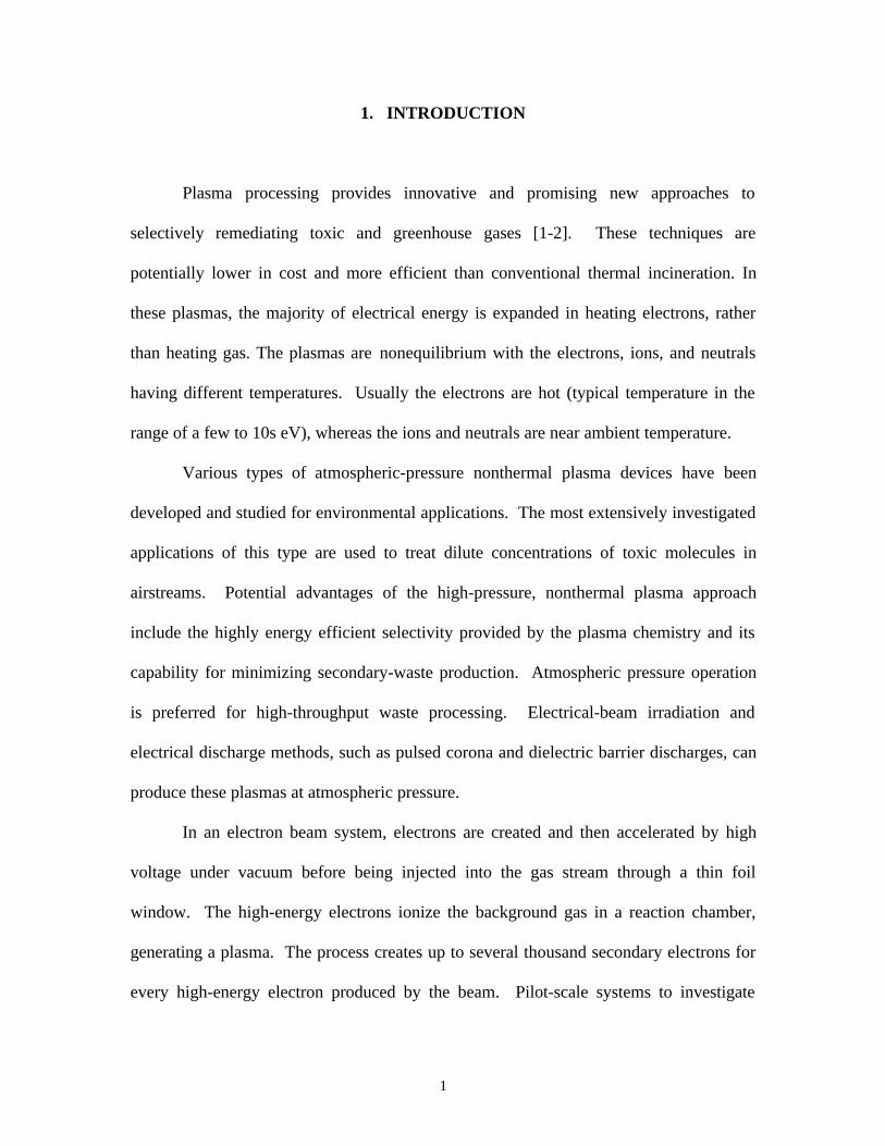
Plasma processing provides innovative and promising new approaches to
selectively remediating toxic and greenhouse gases [1-2]. These techniques are
potentially lower in cost and more efficient than conventional thermal incineration. In
these plasmas, the majority of electrical energy is expanded in heating electrons, rather
than heating gas. The plasmas are nonequilibrium with the electrons, ions, and neutrals
having different temperatures. Usually the electrons are hot (typical temperature in the
range of a few to 10s eV), whereas the ions and neutrals are near ambient temperature.
Various types of atmospheric-pressure nonthermal plasma devices have been
developed and studied for environmental applications. The most extensively investigated
applications of this type are used to treat dilute concentrations of toxic molecules in
airstreams. Potential advantages of the high-pressure, nonthermal plasma approach
include the highly energy efficient selectivity provided by the plasma chemistry and its
capability for minimizing secondary-waste production. Atmospheric pressure operation
is preferred for high-throughput waste processing. Electrical-beam irradiation and
electrical discharge methods, such as pulsed corona and dielectric barrier discharges, can
produce these plasmas at atmospheric pressure.
In an electron beam system, electrons are created and then accelerated by high
voltage under vacuum before being injected into the gas stream through a thin foil
window. The high-energy electrons ionize the background gas in a reaction chamber,
generating a plasma. The process creates up to several thousand secondary electrons for
every high-energy electron produced by the beam. Pilot-scale systems to investigate
2
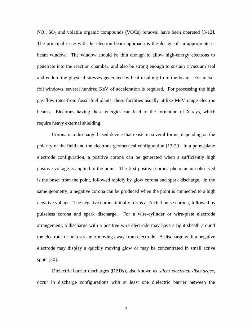
NOx, SO2 and volatile organic compounds (VOCs) removal have been operated [3-12].
The principal issue with the electron beam approach is the design of an appropriate e-
beam window. The window should be thin enough to allow high-energy electrons to
penetrate into the reaction chamber, and also be strong enough to sustain a vacuum seal
and endure the physical stresses generated by heat resulting from the beam. For metal-
foil windows, several hundred KeV of acceleration is required. For processing the high
gas-flow rates from fossil-fuel plants, these facilities usually utilize MeV range electron
beams. Electrons having these energies can lead to the formation of X-rays, which
require heavy external shielding.
Corona is a discharge-based device that exists in several forms, depending on the
polarity of the field and the electrode geometrical configuration [13-29]. In a point-plane
electrode configuration, a positive corona can be generated when a sufficiently high
positive voltage is applied to the point. The first positive corona phenomenon observed
is the onset from the point, followed rapidly by glow corona and spark discharge. In the
same geometry, a negative corona can be produced when the point is connected to a high
negative voltage. The negative corona initially forms a Trichel pulse corona, followed by
pulseless corona and spark discharge. For a wire-cylinder or wire-plate electrode
arrangement, a discharge with a positive wire electrode may have a tight sheath around
the electrode or be a streamer moving away from electrode. A discharge with a negative
electrode may display a quickly moving glow or may be concentrated in small active
spots [30].
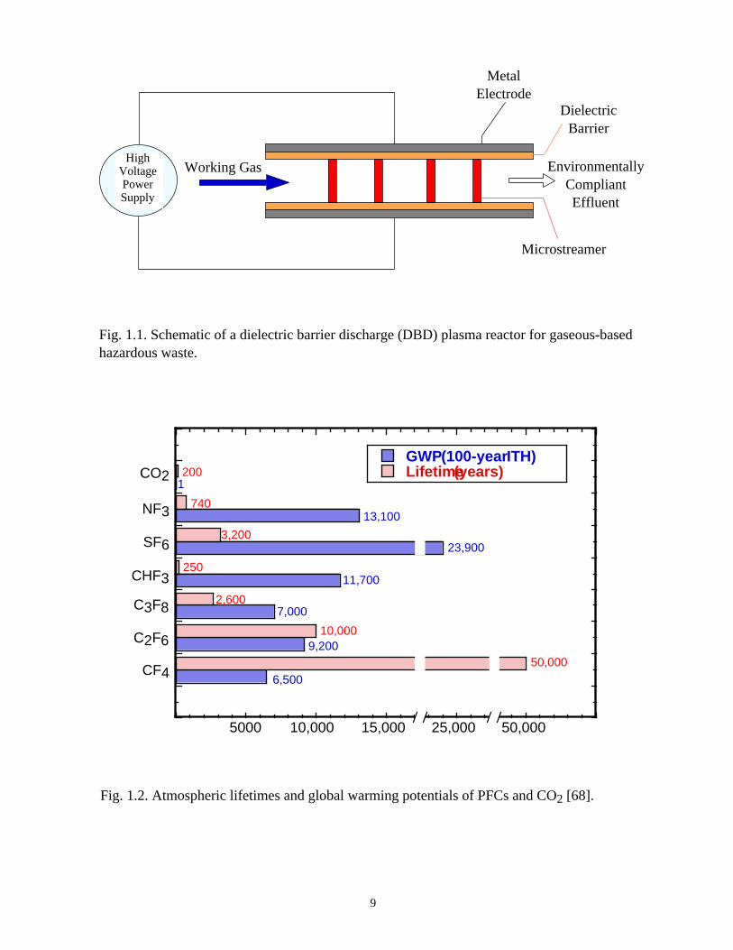
Dielectric barrier discharges (DBDs), also known as silent electrical discharges,
occur in discharge configurations with at least one dielectric barrier between the
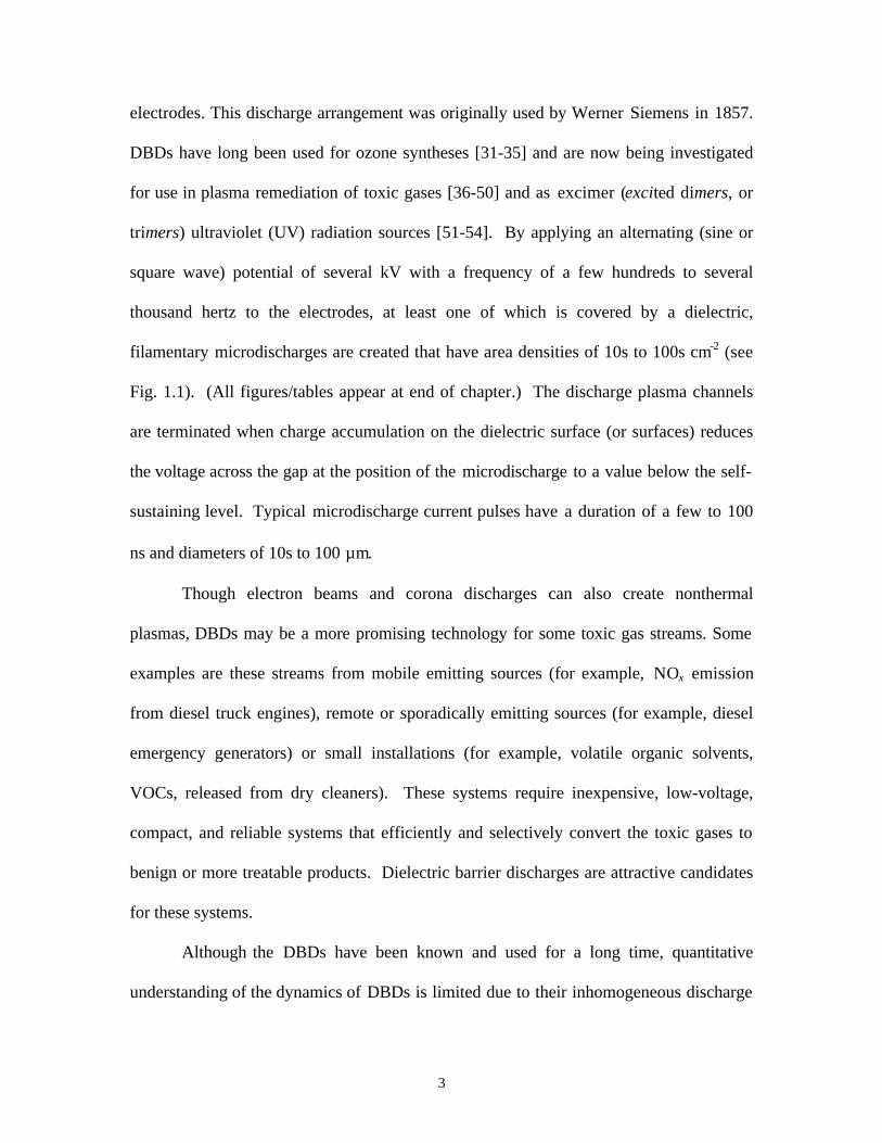
3
electrodes. This discharge arrangement was originally used by Werner Siemens in 1857.
DBDs have long been used for ozone syntheses [31-35] and are now being investigated
for use in plasma remediation of toxic gases [36-50] and as excimer (excited dimers, or
trimers) ultraviolet (UV) radiation sources [51-54]. By applying an alternating (sine or
square wave) potential of several kV with a frequency of a few hundreds to several
thousand hertz to the electrodes, at least one of which is covered by a dielectric,
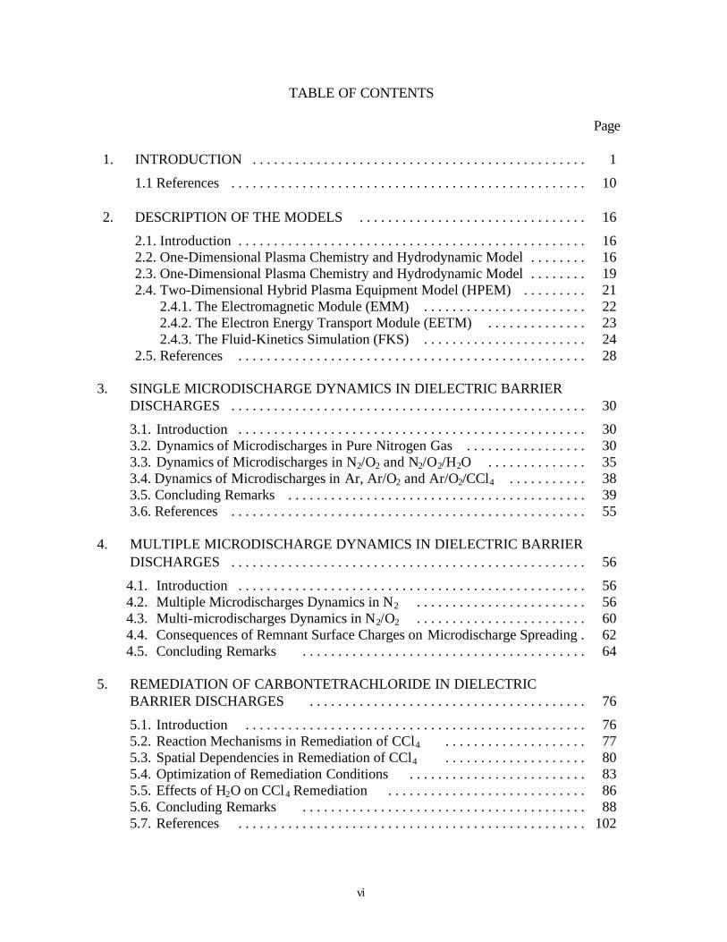
filamentary microdischarges are created that have area densities of 10s to 100s cm-2 (see
Fig. 1.1). (All figures/tables appear at end of chapter.) The discharge plasma channels
are terminated when charge accumulation on the dielectric surface (or surfaces) reduces
the voltage across the gap at the position of the microdischarge to a value below the self-
sustaining level. Typical microdischarge current pulses have a duration of a few to 100
ns and diameters of 10s to 100 µm.
Though electron beams and corona discharges can also create nonthermal
plasmas, DBDs may be a more promising technology for some toxic gas streams. Some
examples are these streams from mobile emitting sources (for example, NOx emission
from diesel truck engines), remote or sporadically emitting sources (for example, diesel
emergency generators) or small installations (for example, volatile organic solvents,
VOCs, released from dry cleaners). These systems require inexpensive, low-voltage,
compact, and reliable systems that efficiently and selectively convert the toxic gases to
benign or more treatable products. Dielectric barrier discharges are attractive candidates
for these systems.
Although the DBDs have been known and used for a long time, quantitative
understanding of the dynamics of DBDs is limited due to their inhomogeneous discharge
4
structures with complex reaction mechanics. Several investigations [33, 55-57] have
computationally addressed microdischarge dynamics in DBDs. One-dimensional
simulations in the direction perpendicular to the electrodes have shown that early during
the discharge pulse the electric field is large in the gap; however, formation of a cathode
fall reduces the bulk electric field, which in turn reduces excitation rates [55-57].
Eliasson and Kogelschatz [33] developed a two-dimensional simulation [(r, z) in the
plane perpendicular to the electrodes] to investigate the expansion of microdischarges
and charging of the dielectric in xenon and oxygen plasmas. They found that for a 1-mm
gap in 1 atm of oxygen, the microdischarge expanded to a radius of 10s to 100s µm in
≈50 ns. Similar computational results were obtained by Braun et al. [57].
In typical applications of DBDs, the gas pressure is sufficiently large (pd > 75 -
100 Torr-cm) and current pulses sufficiently short (<10s ns) that diffusion is not a
dominant process in the ion kinetics. Volumetric processes (ionization, attachment, and
dissociative recombination), which are generally exponentially dependent on the
magnitude of the local electric field, dominantly determine the ion density and mole
fractions. Typically, there is a unique value of E/N (electric field/gas number density) for
a given gas mixture where self-sustaining or steady state ion kinetics can be achieved and
where volumetric ion sources balance volumetric ion sinks. (This is strictly true only for
discharges dominated by attachment and in which multistep processes are not important.)
At a given radial location, as the microdischarge charges the dielectric and removes
voltage from the gap, the electric field in the bulk plasma necessarily transitions from
being above self-sustaining (required to avalanche the gas) to being below self-sustaining
(required to extinguish the discharge). The dependence of rate coefficients on E/N for
5
such things as ionization, attachment, recombination, and ion-ion neutralization can be
markedly different. As a result, the ion kinetics, and therefore ion composition, of the
microdischarge can be expected to be very different as a function of time as the dielectric
charges and E/N changes. This situation is further complicated by the fact that the
microdischarge radially expands during the current pulse from 10s to 100s µm. As the
microdischarge expands, the sequence of avalanche, dielectric charging, and quenching
occurs in a wavelike fashion propagating to larger radii. Ion composition may therefore
depend not only on time but also radius. Since ion chemistry can greatly affect the
efficiency of, for example, plasma remediation processes, the radial dynamics of
microdischarge expansion and their effect on ion chemistry, warrants further study.
To investigate the dynamics and kinetics of plasma remediation in DBDs, one-
dimensional (1-D) and a two-dimensional (2-D) plasma chemistry and hydrodynamics
models have been developed. The 1-D model is radially dependent and is applied to the
study of a single DBD dynamic. The 2-D model is a Cartesian-coordinate simulation
which can be used to investigate dynamics of multiple, radially asymmetric,
microdischarges in close vicinity. The details of the two models are discussed in Chapter
2.
In this work, computer models are used to investigate the dynamics and kinetics
of plasma remediation. In Chapter 3, the 1-D model is applied to the study of ion kinetics
in an expanding microdischarge in a DBD. The context of this study is the use of DBDs
for toxic gas remediation, and therefore, three representative gas systems are
investigated: Ar and N2 (nonattaching); Ar/O2, N2/O2, and N2/O2/H2O (moderately
attaching); and Ar/O2/CCl4 (highly attaching). It was found that as the E/N in the bulk
6
plasma transitions from avalanche to below self-sustaining, the ion kinetics in these three
representative systems differ markedly.
In Chapter 4, results from the 2-D model for the expansion of multiple, closely
spaced microdischarges in DBDs are discussed. Because the final applications of interest
are plasma remediation of toxins from air, N2 and dry air (N2/O2) discharges were
investigated as examples of nonattaching and attaching discharges. Parametric studies
for microdischarge development for one to four adjacent microdischarges are discussed.
Carbon tetrachloride (CCl4) is an important industrial solvent, which is widely
used as degreasing and cleaning agent in the dry-cleaning and textile industries. CCl4 is a
toxin and needs to be carefully disposed of. Several recent experimental studies to
destroy CCl4 have been conducted by using electron-beam irradiation, corona discharges
and dielectric barrier discharges [12, 43, 46, 49]. In Chapter 5, we present an in-depth
study of CCl4 remediation in Ar/O2 and Ar/O2/H2O mixtures in DBDs. The reaction
mechanisms and the optimal conditions are determined.
Another important application of DBDs is to produce narrow-band excimer
ultraviolet radiation. UV photon sources have a number of applications such as
biological sterilization, photochemical degradation of organic compounds in flue gases,
photo-induced surface modification and material deposition, and lithography. During the
last few years DBD UV sources have been investigated using many different excited
species, including rare gas excimers (such as Ar2*, Kr2
*, and Xe2*), molecular rare gas-
halide excimers (such as ArCl*, KrCl*, XeCl*, XeBr*, and XeI*), and halogen dimers
(such as F2*, Cl2
*, Br2* and I2
*), where a wide range of (V)UV spectrum can be covered
7
[51-54, 58, 59]. In Chapter 6, the kinetics and optimization of the XeCl* (308) excimer
system is discussed.
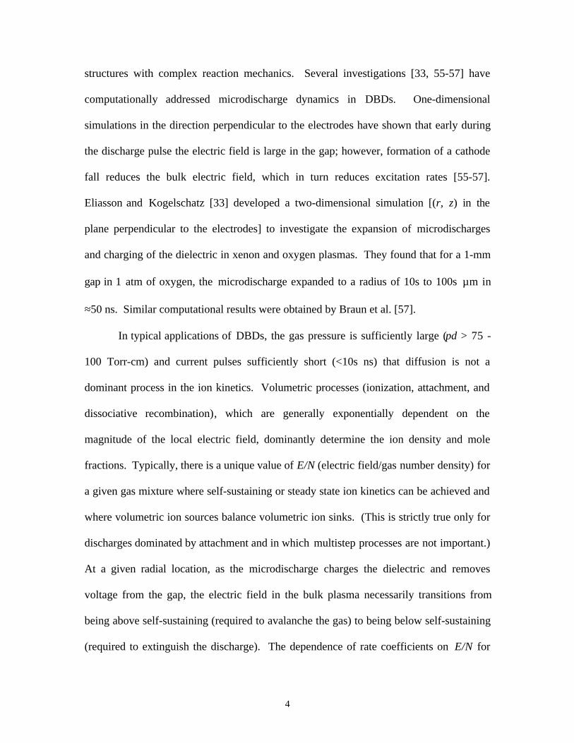
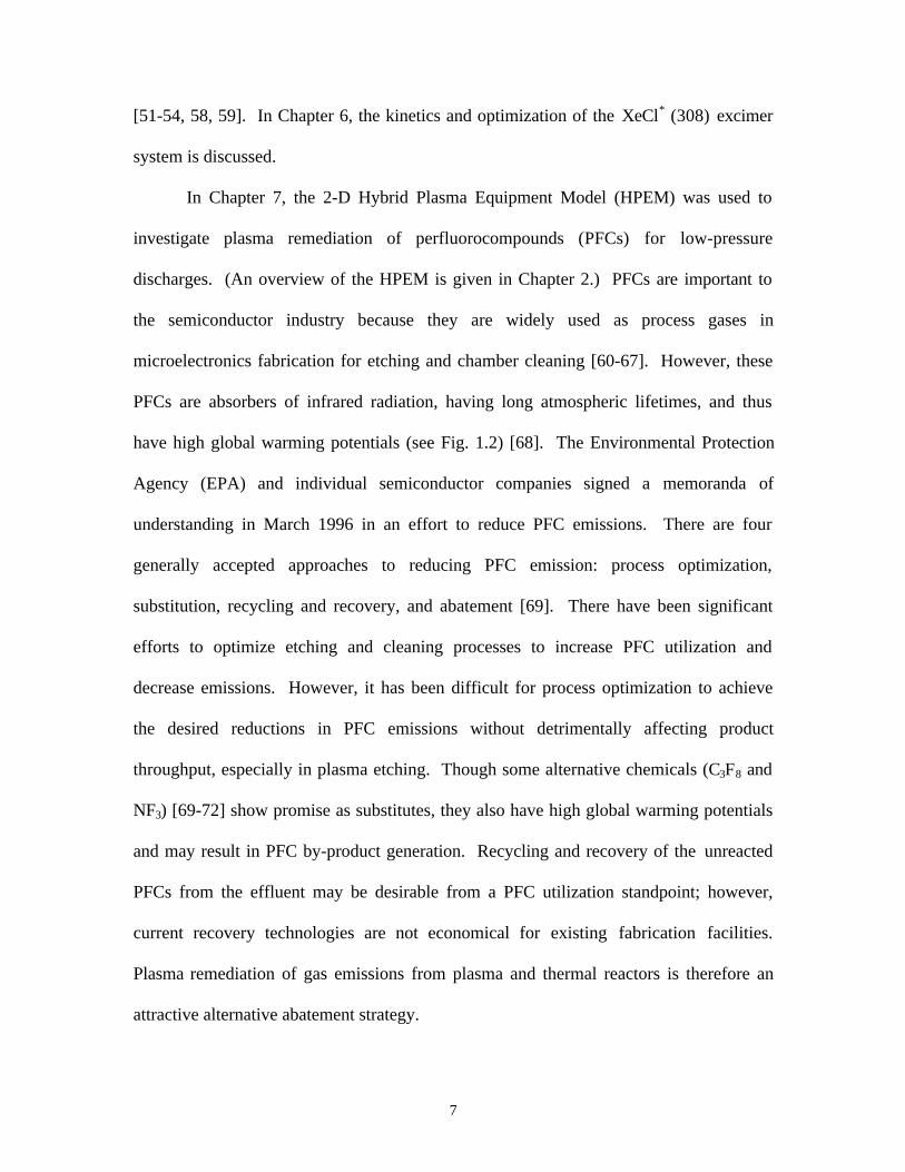
In Chapter 7, the 2-D Hybrid Plasma Equipment Model (HPEM) was used to
investigate plasma remediation of perfluorocompounds (PFCs) for low-pressure
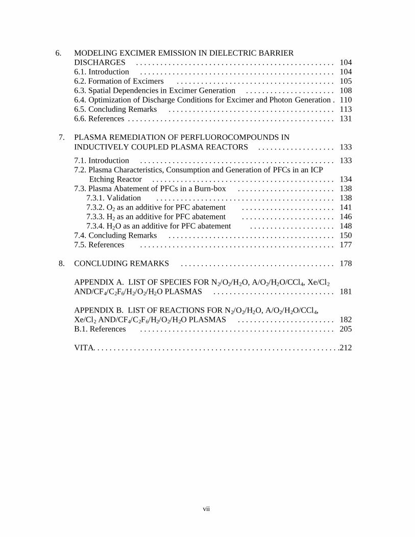
discharges. (An overview of the HPEM is given in Chapter 2.) PFCs are important to
the semiconductor industry because they are widely used as process gases in
microelectronics fabrication for etching and chamber cleaning [60-67]. However, these
PFCs are absorbers of infrared radiation, having long atmospheric lifetimes, and thus
have high global warming potentials (see Fig. 1.2) [68]. The Environmental Protection
Agency (EPA) and individual semiconductor companies signed a memoranda of
understanding in March 1996 in an effort to reduce PFC emissions. There are four
generally accepted approaches to reducing PFC emission: process optimization,
substitution, recycling and recovery, and abatement [69]. There have been significant
efforts to optimize etching and cleaning processes to increase PFC utilization and
decrease emissions. However, it has been difficult for process optimization to achieve
the desired reductions in PFC emissions without detrimentally affecting product
throughput, especially in plasma etching. Though some alternative chemicals (C3F8 and
NF3) [69-72] show promise as substitutes, they also have high global warming potentials
and may result in PFC by-product generation. Recycling and recovery of the unreacted
PFCs from the effluent may be desirable from a PFC utilization standpoint; however,
current recovery technologies are not economical for existing fabrication facilities.
Plasma remediation of gas emissions from plasma and thermal reactors is therefore an
attractive alternative abatement strategy.
8
Plasmas have experimentally demonstrated to efficiently destroy C2F6, a found in
reactor effluent at low pressures. For example, Mohindra et al. [72] used a microwave
tubular reactor to destroy the PFCs. Hartz and coworkers [73] demonstrated the
advantage of utilizing low-pressure surface wave plasmas to destroy C2F6. A commercial
point-of-use RF abatement system developed by Litmas was investigated by Tonnis et al.
[74]. The expansion of the semiconductor industry has resulted in a potential
corresponding increase in PFC emissions, so a need for new methods of PFC remediation
is necessary. It is therefore important to computationally investigate the kinetic processes
of plasma remediation of PFCs in order to optimize the process. In Chapter 7, the
dissociation of PFCs in an inductively coupled plasma (ICP) etching reactor and their
subsequent remediation in a downstream plasma burn-box are discussed.
Finally, conclusions are made in Chapter 8.
HighVoltagePowerSupply
Working Gas EnvironmentallyCompliantEffluent
MetalElectrode
DielectricBarrier
Microstreamer
Fig. 1.1. Schematic of a dielectric barrier discharge (DBD) plasma reactor for gaseous-based hazardous waste.
GWP (100-year ITH)Lifetime (years)
CF4
C2F6
C3F8
CHF3
SF6
NF3
CO2
5000 10,000 15,000 25,000 50,000
6,500
50,0009,200
10,000
2,6007,000
11,700250
23,9003,200
13,100740
2001
Fig. 1.2. Atmospheric lifetimes and global warming potentials of PFCs and CO2 [68].
9
10
1.1 References
[1] Nonthermal Plasma Techniques for Pollution Control, edited by B. N. Penetrante
and S. E. Schultheis (Springer, Berlin, 1993), Parts A and B.
[2] Plasma Science and the Environment, edited by W. Manheimer, L. E. Sugiyama,
T. H. Stix (American Institute of Physics, Woodbury, NY, 1997).
[3] D. J. Helftitch and P. L. Feldman, Radiat. Phys. Chem. 24, 129 (1984).
[4] J. C. Person and D. O. Ham, Radiat. Phys. Chem. 31, 1 (1988)
[5] P. Fuchs, B. Roth, U. Schwing, H. Angele, and J. Gottstein, Radiat. Phys. Chem.
31, 45 (1988).
[6] B. M. Penetrante, M. C. Hsiao, B. T. Merritt, and G. E. Vogtlin, Appl. Phys. Lett.,
66, 3096 (1995).
[7] A. G. Chmielewski, E. Iller, Z. Zemek, M. Romanowski, and K. Koperski, J.
Phys. Chem. 46, 1063 (1995).
[8] L. Prager, H. Langguth, S. Rummel, and R. Mehnert, Radiat. Phys. Chem. 46,
1137 (1995).
[9] S. A. Vitale, K. Hadidi, D. R. Cohn, and L. Bromberg, Radiat. Phys. Chem. 49,
421 (1997).
[10] S. A. Vitale, K. Hadidi, D. R. Cohn, and P. Falkos, Plasma Chem. Plasma
Process, 16, 651 (1996).
[11] N. W. Frank, Radiat. Phys. Chem. 45, 989 (1995).
[12] L. Bromberg, D. R. Cohn, R. M. Patrick, and P. Thomas, Phys. Lett. A 173, 293
(1993).
[13] R. Morrow, Phys. Rev. A32, 1799 (1985).
11
[14] J.-S. Chang, J. Aerosol Sci. 20, 87 (1988).
[15] I. Gallimberti, Pure Appl. Chem. 60, 663 (1988).
[16] S. R. Stearns, J. Appl. Phys. 66, 2899 (1989).
[17] R. J. van Brunt and S. V. Kulkarni, Phys. Rev. A42, 4908 (1990).
[18] P. Pignolet, S. Hadj-Ziane, B. Held, R. Peyrous, J. M. Benas, and C. Coste, J.
Phys. D: Appl. Phys. 14, 1069 (1990).
[19] T. Ohkubo, S. Hamasaki, Y. Nomoto, J. Chang, and T. Adachi, IEEE Trans. Ind.
Appl. 26, 542 (1990).
[20] F. A. van Goor, J. Phys. D: Appl. Phys. 26, 404 (1993).
[21] F. Grange, N. Soulem, J. F. Loiseau, and N. Spyrou, J. Phys. D: Appl. Phys. 28,
1619 (1995).
[22] N. Bonifac, A. Denat, and V. Atrazhez, J. Appl. Phys. 81, 2717 (1997).
[23] A. A. Kulikovsky, IEEE Trans. Plasma Sci. 25 439 (1997).
[24] A. A. Kulikovsky, J. Phys. D: Appl. Phys. 30, 441 (1997).
[25] R. Morrow, J. Phys. D: Appl. Phys. 30, 3099 (1997).
[26] Y. S. Mok, S. W. Ham, and I. S. Nam, IEEE Trans. Plasma Sci. 26, 1566 (1998).
[27] M. Cemak, T. Hosokawa, S. Kobayashi, and T. Kaneda, J. Appl. Phys. 83, 5678
(1998).
[28] M. Simek, V. Babicky, M. Clupek, S. DeBenedictis, G. Dilecce, and P. Sunka, J.
Phys. D: Appl. Phys. 31, 2591 (1998).
[29] S. Kanazawa, J.-S. Chang, G. F. Round, G. Sheng, T. Ohkubo, Y. Nomoto, and T.
Adachi, Combust. Sci. Tech. 133, 93 (1998).
12
[30] J.-S. Chang in Nonthermal Plasma Techniques for Pollution Control, edited by B.
N. Penetrante and S. E. Schultheis (Springer, Berlin, 1993), Part A, pp. 2-32.
[31] B. Eliasson, M. Hirth, and U. Kogelschatz, J. Phys. D.: Appl. Phys., 20, 1421
(1987).
[32] W. Elgi and B. Eliasson, Helvetica Physica Acta 62, 302 (1989).
[33] B. Eliasson and U. Kogelschatz, IEEE Trans. Plasma Sci., 19, 309 (1991).
[34] V. I. Gibalov, J. Drimal, M. Wronski, and V. G. Samoilovich, Contrib. Plasma
Phys. 31, 89 (1991).
[35] J. Kitayama and M Kuzumoto, J. Phys. D.: Appl. Phys., 30, 2453 (1997).
[36] M. B. Chang, J. H. Balbach, M. J. Rood, and M. J. Kushner, J. Appl. Phys., 69,
4409 (1991).
[37] H. Esron and U. Kogelschatz, Appl. Surf. Sci., 54, 440 (1992).
[38] D. Evans, L. A. Rosocha, G. K. Anderson, J. J. Coogan, and M. J. Kushner, J.
Appl. Phys., 74, 5378 (1993).
[39] A. C. Gentile and M. J. Kushner, J. Appl. Phys., 78, 2074 (1995).
[40] A. C. Gentile and M. J. Kushner, J. Appl. Phys., 78, 2977 (1995).
[41] M. C. Hsiao, B. T. Merritt, B. M. Penetrante, and G. E. Voglin, J. Appl. Phys., 78,
3451 (1995).
[42] B. M. Penetrante, M. C. Hsiao, B. T. Merritt, G. E. Vogtlin, Appl. Phys. Lett., 66,
3096 (1995).
[43] B. M. Penetrante, M. C. Hsiao, J. N. Bardsley, B. T. Merritt, G. E. Vogtlin, P. H.
Wallman, A. Kuthi, C. P. Burkhart, and J. R. Bayless, Phys. Lett., 209, 69 (1995).
[44] W. Sun, B. Pashaie, S. K. Dhali, and F. I. Honea, J. Appl. Phys., 79, 3438 (1996).
13
[45] A. C. Gentile and M. J. Kushner, J. Appl. Phys., 79, 3877 (1996).
[46] R. G. Tonkyn, S. E. Barlow, and T. M. Orlando, J. Appl. Phys., 79, 3451 (1996).
[47] Z. Fralkenstein, J. Adv. Oxid. Technol., 1, 1 (1997).
[48] B. M. Penetrante, M. C. Hsiao, J. N. Bardsley, B. T. Merritt, G. E. Vogtlin, A.
Kuthi, C. P. Burkhart, and J. R. Bayless, Plasma Sources. Sci. Technol. 6, 251
(1997).
[49] W. Niessen, O. Wolf, R. Schruft, and M. Neiger, J. Phys. D.: Appl. Phys., 31, 542
(1998).
[50] F. Massines, A. Rabehi, P. Decomps, and R. B. Gadri, J. Appl. Phys., 83, 2950
(1998).
[51] U. Kogelschatz in Nonthermal Plasma Techniques for Pollution Control, edited
by B. N. Penetrante and S. E. Schultheis (Springer, Berlin, 1993), Part B, pp. 339-
354.
[52] J. Zhang and I. W. Boyd, J. Appl. Phys., 80, 633 (1996).
[53] Z. Falkenstein and J. J. Coogan, J. Phys. D.: Appl. Phys., 30, 2704 (1997).
[54] J. Zhang and I W. Boyd, J. Appl. Phys. 84, 1174 (1998).
[55] D. Braun, U. Kuchler, and G. Pietsh, J. Phys. D.: Appl. Phys., 24, 564 (1991).
[56] Y. Sakai, A. Oda, and H. Akashi, Rep. Inst. Fluid Science, 10, 29 (1997).
[57] D. Braun, V. Gibalov, and G. Pietsch, Plasma Sources. Sci. Technol. 1, 166
(1992).
[58] B. Eliasson and U. Kogelschatz, Appl. Phys. B46, 299 (1988).
[59] U. Kogelschatz, Appl. Surf. Sci. 54, 410 (1992).
14
[60] Plasma Etching: An Introduction, edited by D. M. Manos and D. L. Flamm
(Academic, San Diego, CA, 1989).
[61] S. Ito, K. Nakamura, and H. Sugai, Jpn. J. Appl. Phys. 33, L1261 (1994).
[62] P. Verdonck, J. Swart, G. Brasseur, and P. De Geyter, J. Electrochem. Soc. 142,
1971 (1995).
[63] K. Takahashi, M. Hori, and T. Goto, J. Vac. Sci. Technol. A14, 2004 (1996).
[64] A. Tserspi, W. Schwarzenbach, J. Derouard, and N. Sadeghi, J. Vac. Sci. Technol.
A15, 3120 (1997).
[65] M. A. Sobolewski, J. G. Langan and B. S. Felker, J. Vac. Sci. Technol. B16, 173
(1998).
[66] T. E. F. M. Standaert, M. Schaepkens, N. R. Rueger, P. G. M., Sebel, G. S.
Oehrlein, and J. M. Cook, J. Vac. Sci. Technol. A16, 239 (1998).
[67] B. E. E. Kastenmeier, P. J. Matsui, G. S. Oehrlein, and J. G. Langan, J. Vac. Sci.
Technol. A16, 2047 (1998).
[68] L. Beu, P. T. Brown, J. Latt, J. U. Papp, T. Gilliland, T. Tamayo, J. Harrison, J.
Davison, A. Cheng, J. Jewett, W. Worth, Current State of Technology:
Perfluorocompound (PFC) Emissions Reduction, SEMATECH Technology
Transfer 98053508A-TR, 1998.
[69] E. Meeks, R. S. Larson, S. R. Vosen, and J. W. Shon, J. Electrochem. Soc. 144,
357 (1997).
[70] M. Schaekens, G. S. Oehrlein, C. Hedlund, L. B. Jonsson, and H. O. Blom, J.
Vac. Sci. Technol. A16, 3281 (1998).
[71] S. P. Sun, D. Bennett, L. Zazzera, and W. Reagen, Semicond. Int., 85, (1998).
15
[72] V. Mohindra, H. Chae, H. H. Sawin, and M. T. Mocella, IEEE Trans. Semicond.
Manufact., 10, 399 (1997).
[73] C. L. Hartz, J, W. Bevaan, M. W. Jackson, and B. A. Wofford, Environ. Sci.
Technol. 32, 682 (1998).
[74] E. J. Tonnis, V. Vartanian, L. Beu, T. Lii, R. Jewett, and D. Graves, Evaluation of
a Litmas “Blue” Point-of-Use (POU) Plasma Abatement Device for
Perluorocompound (PFC) Destruction, SEMATECH Technology Transfer
98123605A-TR, 1998.
16
2. DESCRIPTION OF THE MODELS
2.1 Introduction
In this chapter, detailed descriptions of the 1-D and the 2-D Plasma Chemistry
and Hydrodynamics Models (PCHMs) for high-pressure DBD processing of gases and
the 2-D Hybrid Plasma Equipment Model (HPEM) for low-pressure plasma abatement
are presented. In Section 2.2, we describe the 1-D PCHM used in Chapter 3 to study ion
kinetics in an expanding microdischarge for a single microdischarge, in Chapter 5 to
investigate CCl4 remediation processing, and in Chapter 6 to examine excimer photon
generation. In Section 2.3, we describe the 2-D PCHM used in Chapter 4 to study the
expansion of multiple, closely spaced microdischarges and the effect of surface
remaining charges on microdischarges in DBDs. In Section 2.4, we describe the 2-D
HPEM used in Chapter 7 to investigate the PFC consumption and generation of PFCs in
an ICP-etching reactor and the abatement of PFCs in a plasma burn box.
2.2 One-Dimensional Plasma Chemistry and Hydrodynamic Model
The model used in this study is a modified version of the 1-D microdischarge
simulation previously discussed in [1]. The model begins by assuming that the DBD is
composed of a uniformly spaced array of identical, radially symmetric microdischarges.
The numerical mesh is discretized in the radial direction with varying resolution from
submicron near the center to a few microns at the outer radius. The last numerical cell
has a square outer boundary and circular inner boundary in order to apply reflective
boundary conditions. The spacing of the microdischarges is sufficiently large that they
17
do not significantly interact, and therefore, a single microdischarge employing reflective
boundary conditions can be used. Typically 800-900 radial points are used in the
simulation.
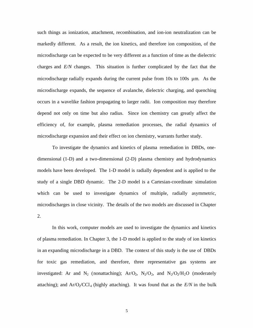
The model is composed of four components: an external circuit model, a solution
of Boltzmann's equation for the electron energy distribution, a heavy plasma chemistry
model, and a transport module. A schematic of the modules of PCHM is shown in Fig.
2.1. The external circuit model calculates the voltage across the plasma, which is then
used to obtain the time evolution of the electron energy distribution from the solution of
Boltzmann's equation. The heavy particle plasma chemistry model produces the
concentrations of neutral and charged particles, and also provides the plasma conductivity
for the external circuit model. The motion of species between mesh points is addressed
in the transport module. Electron impact rate coefficients for use in the plasma chemistry
model are obtained using the local field approximation. Solutions of Boltzmann’s
equation [2] are parameterized over a wide range of E/N, and the resulting rate and
electron impact rate coefficients are placed in a look-up table for use during execution of
the model.
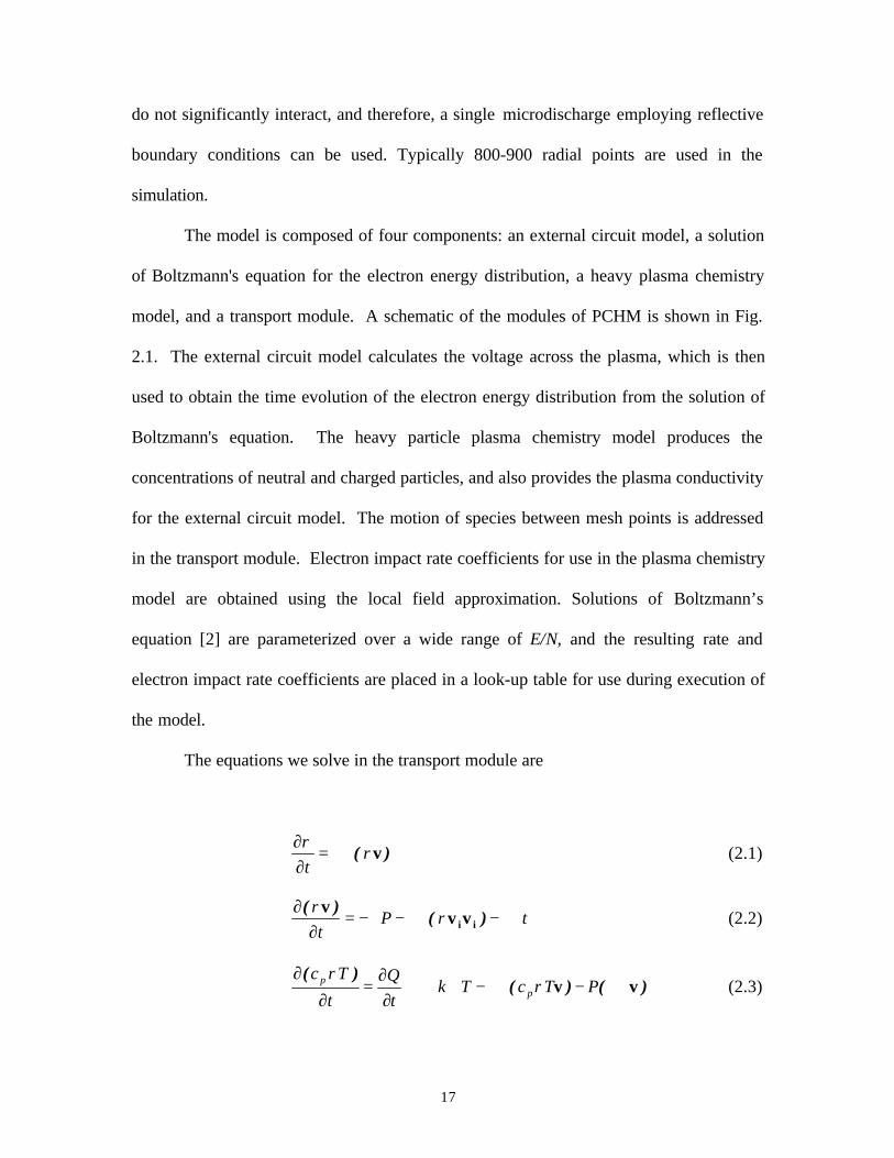
The equations we solve in the transport module are
)( vρρ
⋅∇=∂∂
t (2.1)
τρρ
⋅∇−⋅∇−−∇=∂
∂)(
)(iivv
vP
t (2.2)
)()()(
vv ⋅∇−⋅∇−∇⋅∇+∂∂
=∂
∂PTcT
t
Q
t
Tcp
p ρκρ
(2.3)
18
where ρ is the mass density, v is the velocity, T is the temperature, cp is the heat capacity,
P is the thermodynamic pressure (assuming ideal gas behavior), τ is the viscosity tensor,
Q is the enthalpy, and κ is the thermal conductivity. The form of the viscosity tensor
used is given by Thompson [3]. The viscosity and thermal conductivity of the gas was
obtained using Lennard Jones parameters and applying the mixture rules as described in
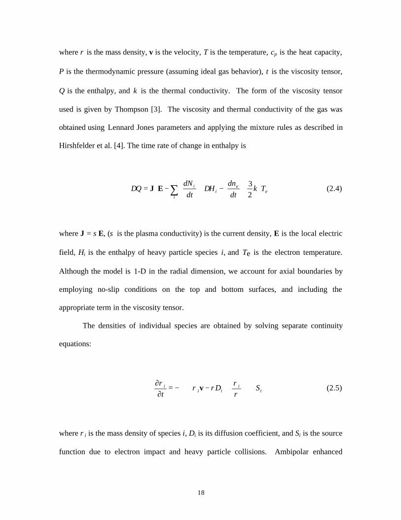
Hirshfelder et al. [4]. The time rate of change in enthalpy is
ee
ii
i Tkdt
dnH
dt
dNQ ⋅⋅
−⋅
−⋅= ∑ 2
3∆∆ EJ (2.4)
where J = σE, (σ is the plasma conductivity) is the current density, E is the local electric
field, Hi is the enthalpy of heavy particle species i, and Te is the electron temperature.
Although the model is 1-D in the radial dimension, we account for axial boundaries by
employing no-slip conditions on the top and bottom surfaces, and including the
appropriate term in the viscosity tensor.
The densities of individual species are obtained by solving separate continuity
equations:
ii
iii SD
t+
∇−⋅−∇=∂
∂ρρρρρ
v (2.5)
where ρi is the mass density of species i, Di is its diffusion coefficient, and Si is the source
function due to electron impact and heavy particle collisions. Ambipolar enhanced
19
diffusion coefficients are used for ions. The transport equations were explicitly
integrated in time using a fourth-order Runga-Kutta-Gill technique. Spatial derivatives
are formulated using conservative finite difference donor cell techniques on a staggered
mesh (ρ and T are obtained at cell vertices whereas ρv is obtained at cell boundaries). In
addition, a finite surface conductivity for the dielectric was used in order to simulate the
spreading of charge on the dielectric surface.
2.3 Two-Dimensional Plasma Chemistry and Hydrodynamic Model
The 2-D model of DBDs used in this study is analog to the 1-D model described
above. We resolve the two dimensions parallel to the electrodes and therefore do not
address the cathode fall dynamics. This model addresses the positive column
characteristics of the microdischarge. To begin, we select a gas mixture, gap spacing,
dielectric properties, and voltage pulse shape. A small initial electron density (108-109
cm-3), having a radial extent of a few microns, is specified as an initial condition. The
voltage pulse is applied, and the compressible Navier-Stokes equations are solved for
continuity, momentum conservation, and energy density of the gas mixture. Continuity
equations are solved for all heavy particle species (neutrals and ions) and electrons. We
invoke the local field approximation for electron transport. In doing so, the electron
transport coefficients are obtained from the spatially dependent value of E/N and a two-
term spherical harmonic solution of Boltzmann’s equation.
The transport equations were explicitly integrated in time using a fourth-order
Runga-Kutta-Gill technique. Spatial derivatives are formulated using conservative finite
difference donor cell techniques on a staggered mesh (ρ[mass density] and T
20
[temperature] are solved for at cell vertices, whereas ρv[momentum] is obtained at cell
boundaries). The 2-D mesh was rectilinear with (usually) equal spacing in each
direction. In the cases where we have bulk gas flow through the device (e.g., a “right to
left” flow field), we simply superimposed a bulk flow velocity vb parallel to the
electrodes. To account for no-slip flow and formation of boundary layers in the axial
direction, we include an axial sheer term in the viscous drag term of the momentum
equation. This term is formulated using Λ = d/π (d is the gap spacing) as the transport
length. The axial electrical field is also provided by solving circuit equations for the
pulse power apparatus and dielectric charging. Given the E/N in the plasma, electron
impact rate coefficients are obtained using the local field approximation from a two-term
spherical harmonic expansion of Boltzmann’s equation for the electron energy
distribution. In the plasma chemistry model, the densities for all species, the gas
temperature, and the charge density on the dielectric are updated independently at each
mesh point while excluding transport. This method allow us to use a different integration
time step at each mesh point, which tends to be shorter (<10-11 s) in the active
microdischarge region and longer outside the microdischarge. After the update of the
local kinetics, the densities are then updated based on advection and diffusion in the
hydrodynamic model where the momentum equations are simultaneously solved. We
enforced electrical neutrality, so the electron density at each mesh point is forced to be
equal to the charge weighted sum of the ion densities.
Initial conditions are generated by specifying (or randomly distributing) a center
point for each microdischarge in the 2-D domain. The microdischarge is assumed to be
21
initially radially symmetric and composed of a seed electron density having a super-
Gaussian profile.
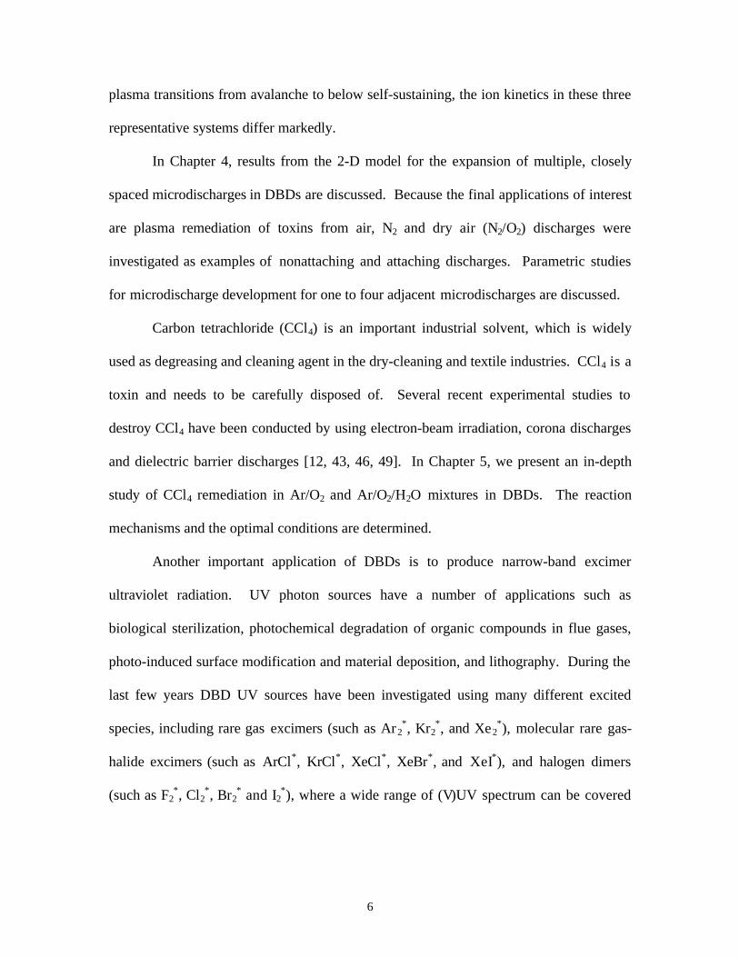
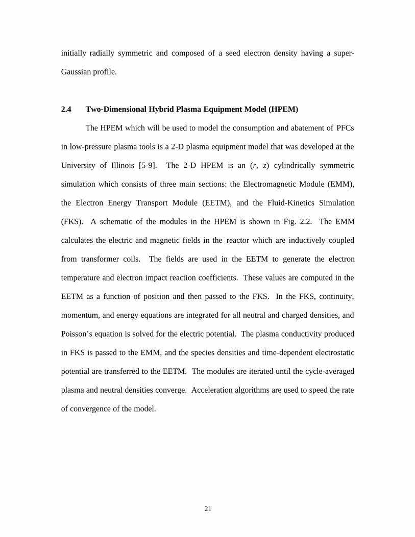
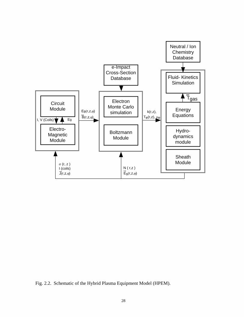
2.4 Two-Dimensional Hybrid Plasma Equipment Model (HPEM)
The HPEM which will be used to model the consumption and abatement of PFCs
in low-pressure plasma tools is a 2-D plasma equipment model that was developed at the
University of Illinois [5-9]. The 2-D HPEM is an (r, z) cylindrically symmetric
simulation which consists of three main sections: the Electromagnetic Module (EMM),
the Electron Energy Transport Module (EETM), and the Fluid-Kinetics Simulation
(FKS). A schematic of the modules in the HPEM is shown in Fig. 2.2. The EMM
calculates the electric and magnetic fields in the reactor which are inductively coupled
from transformer coils. The fields are used in the EETM to generate the electron
temperature and electron impact reaction coefficients. These values are computed in the
EETM as a function of position and then passed to the FKS. In the FKS, continuity,
momentum, and energy equations are integrated for all neutral and charged densities, and
Poisson’s equation is solved for the electric potential. The plasma conductivity produced
in FKS is passed to the EMM, and the species densities and time-dependent electrostatic
potential are transferred to the EETM. The modules are iterated until the cycle-averaged
plasma and neutral densities converge. Acceleration algorithms are used to speed the rate
of convergence of the model.
22
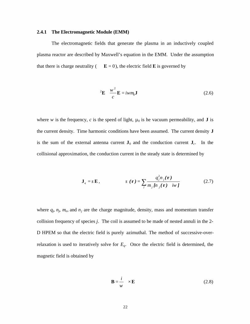
2.4.1 The Electromagnetic Module (EMM)
The electromagnetic fields that generate the plasma in an inductively coupled
plasma reactor are described by Maxwell’s equation in the EMM. Under the assumption
that there is charge neutrality ( 0=⋅∇ E ), the electric field E is governed by
JEE 0
22 ωµ
ωi
c=+∇ (2.6)
where ω is the frequency, c is the speed of light, µ0 is he vacuum permeability, and J is
the current density. Time harmonic conditions have been assumed. The current density J
is the sum of the external antenna current J0 and the conduction current Jc. In the
collisional approximation, the conduction current in the steady state is determined by
EJ c σ= , ∑ +=
j jj
jj
im
nq
])([
)()(
ωνσ
r
rr
2
(2.7)
where qj, nj, me, and ν j are the charge magnitude, density, mass and momentum transfer
collision frequency of species j. The coil is assumed to be made of nested annuli in the 2-
D HPEM so that the electric field is purely azimuthal. The method of successive-over-
relaxation is used to iteratively solve for Eθ. Once the electric field is determined, the
magnetic field is obtained by
EB ×∇=ωi
(2.8)
23
2.4.2 The Electron Energy Transport Module (EETM)
There are two methods for determining the electron energy distribution (EED) as
a function of position in EETM. The first one is by solving the Boltzmann and electron
energy conservation equations in Boltzmann-electron energy equation module (BEM).
The second method uses the electron Monte Carlo simulation (EMCS) for spatially
varying EED.
In the BEM, Boltzmann’s equation is solved using a two-term spherical harmonic
expansion for a range of the reduced electric field E/N as follows:
eee
ee
e ffm
qf
t
fν−=∇⋅×++∇⋅+
∂∂
vBvEv )()( (2.9a)
10 eee fv
ffv
+= (2.9b)
where fe is the electron distribution function, ν is the electron momentum transfer
collision frequency, qe is the electron charge, E is the electric field, and B is the magnetic
field. A table of electron transport properties as a function of electron temperature is
created. The interpolated data are used in solving electron energy equation as follows;
( )
∇−⋅∇−−=
∂
∂
∑ eebi
iiee
ebe
TTkkNnTPt
TknλΓΓ
2
52
3
(2.10)
where Te is the electron temperature, ne is the electron density, P is the electron power
deposition, kb is Boltzmann’s constant, ki is the rate coefficient of power loss for
24
collisions of electrons with species i having density Ni, λ is the electron thermal
conductivity, and ΓΓ is the electron flux. This equation is solved in the steady state using
successive over relaxation. Finally the electron transport coefficients such as electron
impact rate coefficients, source terms for electrons and ions, and transport coefficients are
updated using the spatially dependent electron temperature.
The alternative method for determining the electron transport and energy
properties is used by EMCS. The electron EMCS is executed using a few thousand
pseudoparticles. Electrons are initialized as a Maxwellian velocity distribution and
distributed in the reactor weighted by the electron density from the FKS. The particle
trajectories are simulated under a Lorentzian force from the local electric and magnetic
fields as a function of time. The EMCS is performed for ≈ 20−50 RF cycles for each
iteration. The resulting time-averaged electron energy distribution is used to generate
electron impact source functions for each process.
2.4.3. The Fluid-Kinetics Simulation (FKS)
The FKS solves the fluid transport equations for all charged and neutral species
with chemical and electron impact reactions and Poisson’s equation or an ambipolar field
solution for the electrostatic potential. Electron density and flux are obtained by solving
the drift-diffusion equations. For all other charged and neutral species, we solve the
species continuity, momentum, and energy equations as follows
iii Snt
n+⋅−∇=
∂∂
)( iv (2.11)
25
i
iii
i
iiii
m
nqn
m
kTn
t
n ))(
)()( sii
E(Evv
v ++⋅∇−
∇−=
∂∂
)( ijijjij ji
j nnmm
mvv −
++ ∑ ν (2.12)
222
Em
qnnP
t
n
ii
iiiiii
ji
)()(
)() ων
νε
ε
++⋅∇−⋅∇−⋅−∇=
∂
∂iii vvQ
∑ −+
++j
ijijjiji
ijs
ii
ii TTknnmm
mE
m
qn)(ν
ν32
2
(2.13)
where ni, vi, mi, Ti, qi, εi, Qi, Pi, and νi, are, respectively, the number density, velocity,
mass, temperature, charge, thermal energy, thermal flux, pressure, and momentum
transfer collision frequency of species i. Si is the source function for species i resulting
from heavy particle and electron impact collision. The parameter νij is the rate constant
for the collision between species i and j, mij = mimj/(mi + mj) is the reduced mass, and k is
Boltzmann’s constant. Equations (2.11) and (2.12) are solved in space and time, while
Equation (2.13) is solved only in the steady state because the time scale of the energy
equation is several orders of magnitude longer than other plasma time scales. The
average gas temperature, which is a density weighed average of neutral species, is
computed for chemical reactions which are dependent on temperature.
At sufficiently high pressures, gas atoms achieve thermal equilibrium with
surfaces they come in contact with. The gas and surface temperature are, therefore,
essentially the same at the interface. However, at low pressures there might not be
sufficient numbers of collisions to efficiently couple the gas and adjacent surfaces,
resulting in a temperature difference. This condition is known as the temperature jump
26
effect [10-12]. Because ICPs generally operate at low pressures (<10s mTorr), a
temperature jump at reactor walls is accounted for using the method developed by
Kennard [10]. Using this method, the difference between the wall temperature Tw and the
gas temperature Tg at the wall are given by
x
TgTT g
gw ∂
∂=− . (2.14)
The temperature Tg and its derivative are computed at the wall. The factor g is
( )( )( ) λγα
γα12
592
+−−
=g , (2.15)
where α, γ , and λ are, respectively, the accommodation coefficient, ratio of specific
heats, and mean free path. The accommodation coefficient determines how well the gas
thermally couples to the surface and its value varies from 0 (no coupling) to 1 (perfect
coupling). The actual value depends on the gas and condition of the surface.
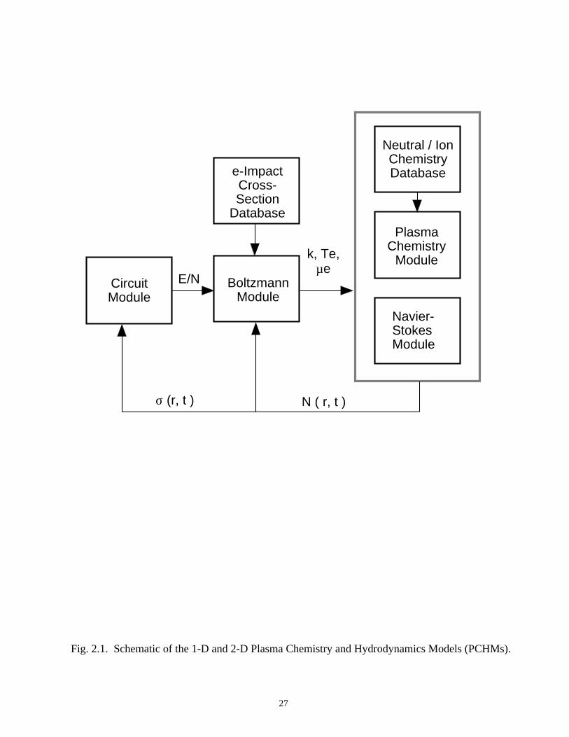
Fig. 2.1. Schematic of the 1-D and 2-D Plasma Chemistry and Hydrodynamics Models (PCHMs).
27
CircuitModule
BoltzmannModule
Neutral / IonChemistryDatabase
k, Te,µe
N ( r, t )σ (r, t )
E/N
e-ImpactCross-Section
Database
Navier-StokesModule
PlasmaChemistry
Module
CircuitModule
k(r,z),Te(r,z), µe
N ( r,z )σ (r, z )I (coils)
Electro-MagneticModule
I, V (Coils) Eθ
e-ImpactCross-Section
Database
BoltzmannModule
ElectronMonte CarlosimulationEθ(r,z,φ)
B(r,z,φ)
Neutral / IonChemistryDatabase
SheathModule
Fluid- KineticsSimulation
EnergyEquations
Hydro-dynamicsmodule
Tgas
J(r,z,φ) Es(r,z,φ)
Fig. 2.2. Schematic of the Hybrid Plasma Equipment Model (HPEM).
28
29
2.5 References
[1] A. C. Gentile and M. J. Kushner, J. Appl. Phys., 79, 3877 (1996).
[2] S. D. Rockwood, Phys. Rev. A., 6, 2348 (1993).
[3] P. A. Thompson, Compressible Fluid Dynamics (McGraw-Hill, NY, 1972), p. 9
and Appendix E.
[4] J. O. Hirschfelder, C. F. Curtiss, and R. B. Bird, in Molecular Theory of Gases
and Liquids (Wiley, New York, 1954), Chap. 8.
[5] P. L. G. Ventzek, R. J. Hoekstra, and M. J. Kushner, J. Vac. Sci. Technol. B. 12,
461 (1994).
[6] W. Z. Collison and M. J. Kushner, Appl. Phys. Lett. 68, 903 (1996).
[7] S. Rauf and M. J. Kushner, J. Appl. Phys. 82, 2805 (1997).
[8] M. J. Grapperhaus, Z. Krivokapic, and M. J. Kushner, J. Appl. Phys. 83, 35
(1998).
[9] S. Rauf and M. J. Kushner, J. Appl. Phys. 83, 5087 (1998).
[10] E. H. Kennard, Kinetic Theory of Gases (McGraw-Hill, NY, 1938).
[11] Y. Sone, T. Ohwada, and K. Aoki, Phys. Fluids A 1, 363 (1989).
[12] S. K. Loyalka, Physica A 163, 813 (1990).
30
3. SINGLE MICRODISCHARGE DYNAMICS IN DIELECTRIC BARRIERDISCHARGES
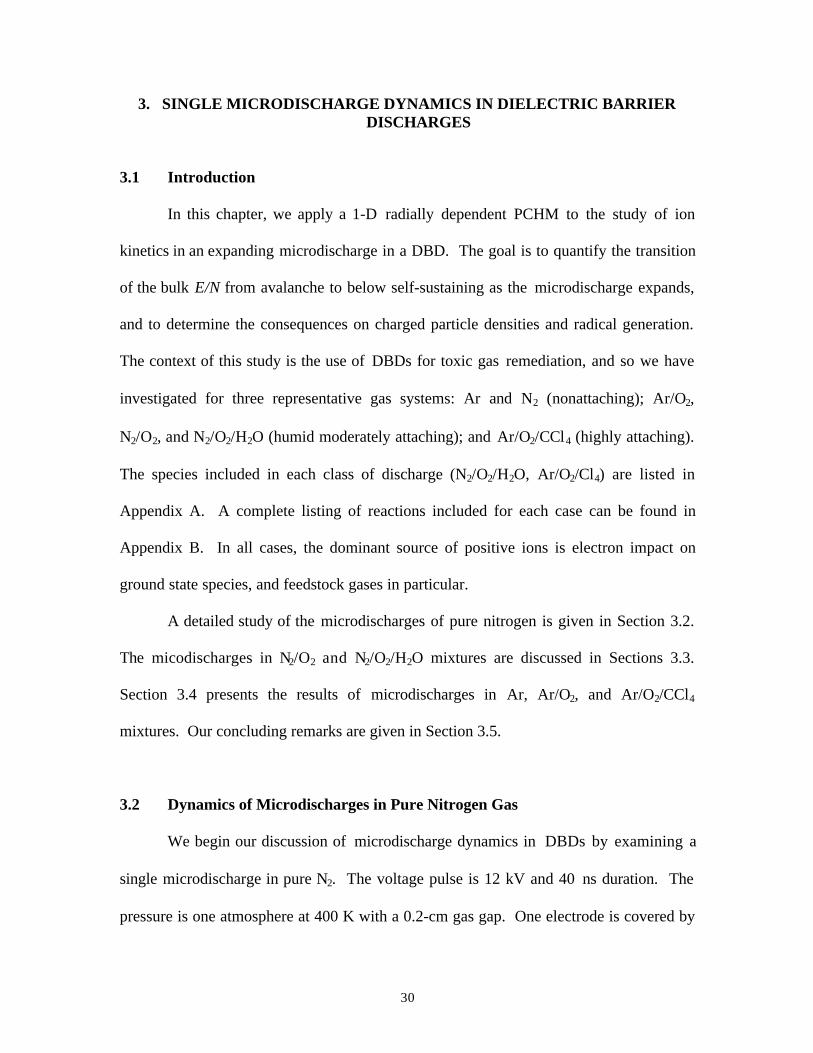
3.1 Introduction
In this chapter, we apply a 1-D radially dependent PCHM to the study of ion
kinetics in an expanding microdischarge in a DBD. The goal is to quantify the transition
of the bulk E/N from avalanche to below self-sustaining as the microdischarge expands,
and to determine the consequences on charged particle densities and radical generation.
The context of this study is the use of DBDs for toxic gas remediation, and so we have
investigated for three representative gas systems: Ar and N2 (nonattaching); Ar/O2,
N2/O2, and N2/O2/H2O (humid moderately attaching); and Ar/O2/CCl4 (highly attaching).
The species included in each class of discharge (N2/O2/H2O, Ar/O2/Cl4) are listed in
Appendix A. A complete listing of reactions included for each case can be found in
Appendix B. In all cases, the dominant source of positive ions is electron impact on
ground state species, and feedstock gases in particular.
A detailed study of the microdischarges of pure nitrogen is given in Section 3.2.
The micodischarges in N2/O2 and N2/O2/H2O mixtures are discussed in Sections 3.3.
Section 3.4 presents the results of microdischarges in Ar, Ar/O2, and Ar/O2/CCl4
mixtures. Our concluding remarks are given in Section 3.5.
3.2 Dynamics of Microdischarges in Pure Nitrogen Gas
We begin our discussion of microdischarge dynamics in DBDs by examining a
single microdischarge in pure N2. The voltage pulse is 12 kV and 40 ns duration. The
pressure is one atmosphere at 400 K with a 0.2-cm gas gap. One electrode is covered by
31
0.5 mm thickness of a dielectric having permittivity of 5εo. The initial seed electron
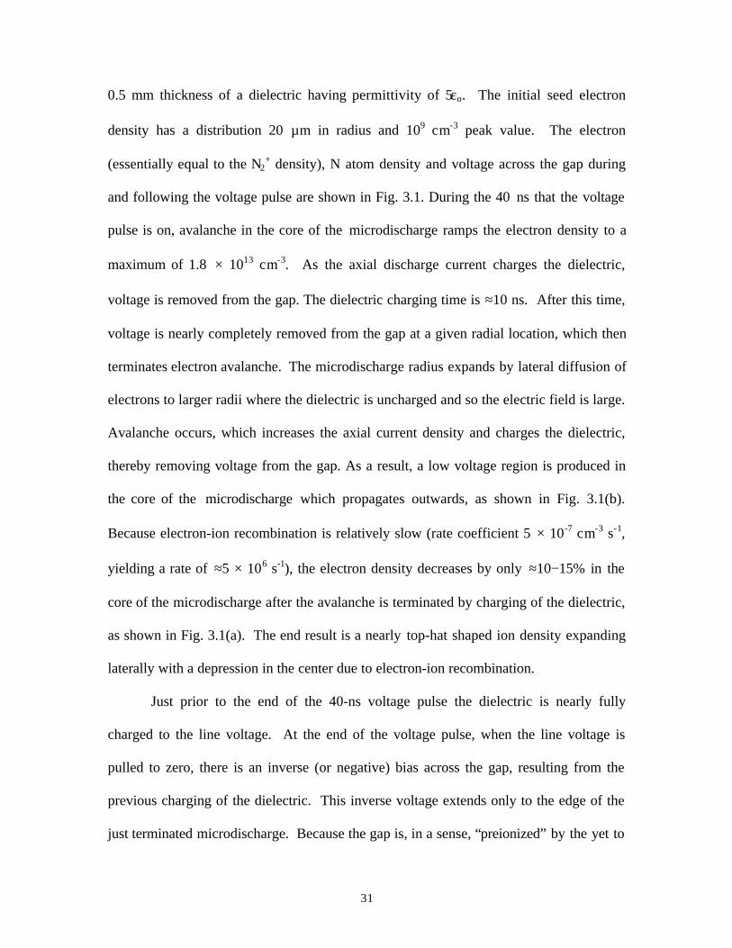
density has a distribution 20 µm in radius and 109 cm-3 peak value. The electron
(essentially equal to the N2+ density), N atom density and voltage across the gap during
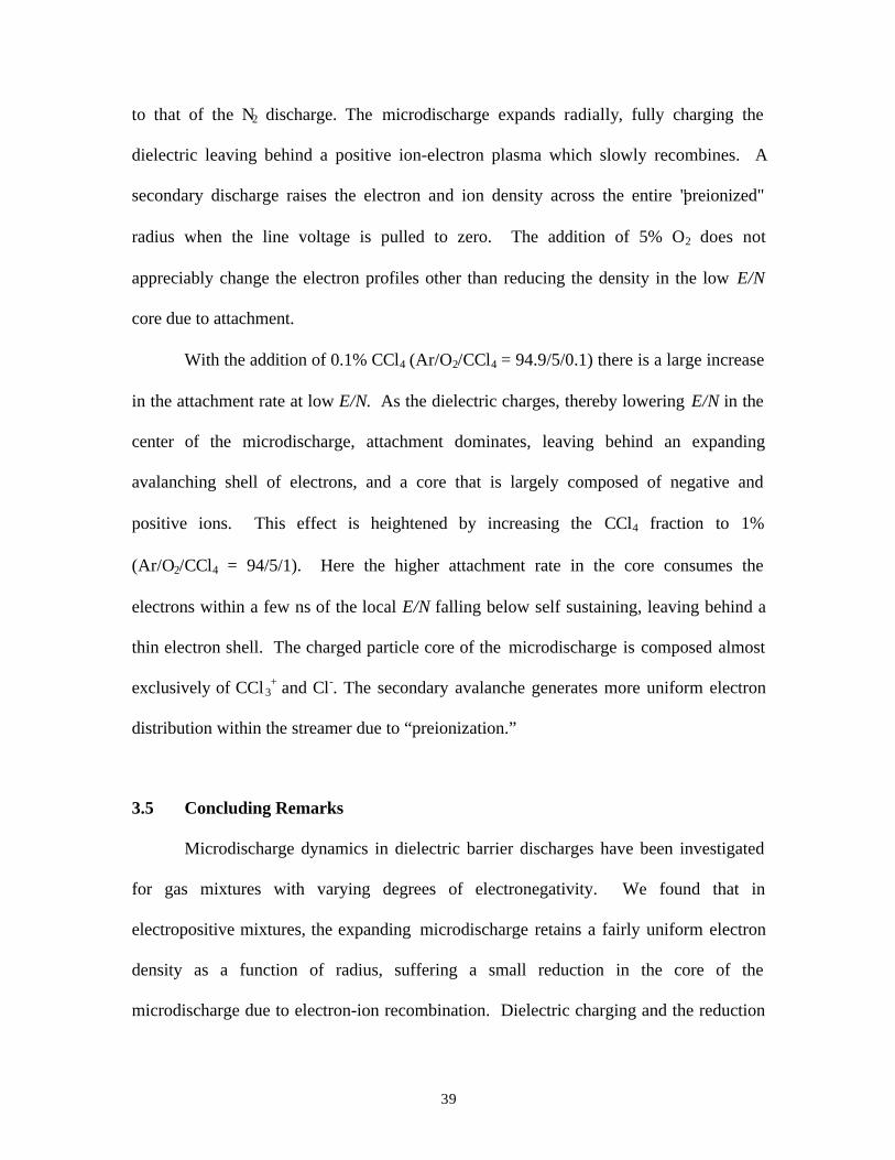
and following the voltage pulse are shown in Fig. 3.1. During the 40 ns that the voltage
pulse is on, avalanche in the core of the microdischarge ramps the electron density to a
maximum of 1.8 × 1013 cm-3. As the axial discharge current charges the dielectric,
voltage is removed from the gap. The dielectric charging time is ≈10 ns. After this time,
voltage is nearly completely removed from the gap at a given radial location, which then
terminates electron avalanche. The microdischarge radius expands by lateral diffusion of
electrons to larger radii where the dielectric is uncharged and so the electric field is large.
Avalanche occurs, which increases the axial current density and charges the dielectric,
thereby removing voltage from the gap. As a result, a low voltage region is produced in
the core of the microdischarge which propagates outwards, as shown in Fig. 3.1(b).
Because electron-ion recombination is relatively slow (rate coefficient 5 × 10⁻⁷ cm-3 s-1,
yielding a rate of ≈5 × 10⁶ s-1), the electron density decreases by only ≈10−15% in the
core of the microdischarge after the avalanche is terminated by charging of the dielectric,
as shown in Fig. 3.1(a). The end result is a nearly top-hat shaped ion density expanding
laterally with a depression in the center due to electron-ion recombination.
Just prior to the end of the 40-ns voltage pulse the dielectric is nearly fully
charged to the line voltage. At the end of the voltage pulse, when the line voltage is
pulled to zero, there is an inverse (or negative) bias across the gap, resulting from the
previous charging of the dielectric. This inverse voltage extends only to the edge of the
just terminated microdischarge. Because the gap is, in a sense, “preionized” by the yet to
32
fully recombine plasma, there is a secondary rapid avalanche that nearly doubles the peak
ion density. Because the electron density in the microdischarge is large compared to the
initial density prior to the primary avalanche, discharging the dielectric is more rapid
(≈2.6 ns) and occurs nearly simultaneously across the entire radius. Any lateral diffusion
of electrons, of which there is a small component, does not significantly expand the
microdischarge. The "stationary" microdischarge results from the fact that for the
secondary avalanche, the gap voltage beyond the boundary of the microdischarge is zero,
whereas for the primary avalanche, the gap voltage is always largest outside the
microdischarge. After the short secondary avalanche, the electron and ion density
continue their slow decrease by dissociative recombination.
The N atom density resembles the ion density as a function of position and time.
N atoms, produced by electron impact dissociation of N2, accumulate during the current
pulse since the rate of reassociation to form N2 (or ionization to form N+) is slow. The
radial profile of the N atom density is even more uniform than for the ions since the
volumetric sink terms and rate of radial diffusion are both smaller.
It was found that the energy deposition and peak electron density in the
microdischarge increased nearly linearly with increasing the dielectric capacitance (either
by increasing ε or decreasing thickness) for a given line voltage. The maximum
microdischarge radius, however, is a weak function of dielectric properties and energy
deposition, provided that the line voltage is constant. We found that the rate of expansion
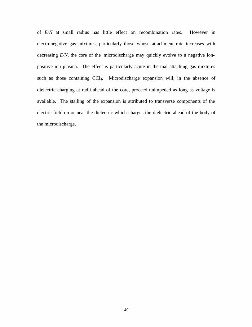
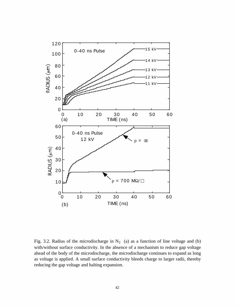
of the microdischarge radius depends most sensitively on the line voltage. In agreement
with Eliasson and Kogelschatz [1], we found that the rate of microdischarge expansion is
largely a function of the rate of electron avalanche, which for our conditions increases
33
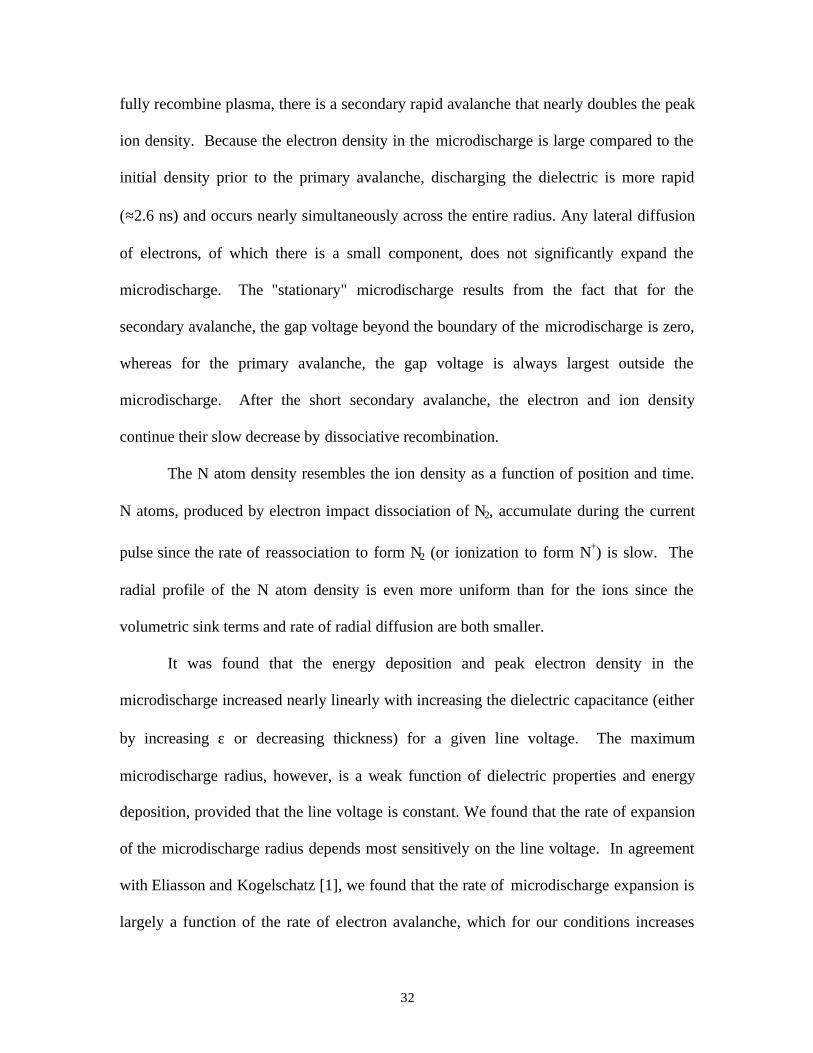
with increasing voltage. This trend is shown in Fig. 3.2(a) where the microdischarge
radius is plotted as a function of time for increasing charging voltage during a 40 ns
pulse. The microdischarge radius increases nearly linearly with time after the first 5-10
ns. The short induction time is the duration required for electron avalanche to increase
the axial current to the magnitude required to fully charge the dielectric, and collapses the
gap voltage in the center of the microdischarge. This induction time increases with
decreasing line voltage.
In the absence of there being a mechanism to charge the dielectric at larger radii
than the expanding microdischarge, a process which removes voltage from the gap, the
microdischarge will continue to grow as long as the voltage is on. (Under conditions of
high energy deposition, hydrodynamic effects that rarefy the microdischarge core and
“snow plow” a high gas density shell will reduce the E/N at large radius and eventually
terminate expansion [2]. The energy deposition in these cases is insufficient for this to
occur.) The experimental observation is that the expansion of the microdischarge stalls
after 10-30 ns, which conflicts with these results.
In the two-dimensional modeling results of Eliasson and Kogelschatz, in which
the electric potential is obtained from solving Poisson's equation in the (r, z) plane,
charging of the dielectric produced a lateral component of the electric field [1]. This
lateral component redirected charge flowing to the dielectric to radii greater than the
main body of the microdischarge. The reduced gap voltage at large radii (or lengthened
field lines) lowered ionization rates sufficiently to stall expansion. In our one-
dimensional model, we can capture this behavior by allowing a finite surface
conductivity (or less than infinite surface resistance) for the dielectric. The finite surface
34
resistance allows the charge on the dielectric to spread laterally to larger radii than the
microdischarge region. As a result, the gap voltage at large radii is eventually reduced to
values lower than that required for avalanche and stalls the expansion of the
microdischarge during the voltage pulse. For example, the microdischarge radius is
shown in Fig. 3.2(b) as a function of time for a 12-kV pulse with and without surface
conductivity. The expansion of the microdischarges is similar in the initial stage (< 4-5
ns). Lateral charging of the dielectric when there is a nonzero surface conductivity,
however, essentially halts the expansion after ≈5 ns. Further expansion is slow, although
there is some small amount of additional microdischarge growth during the secondary
avalanche. In the case of there being no surface conductivity, the microdischarge
expands as long as there is voltage across the gap.
The peak gas temperature in the microdischarge depends on the total energy
deposition, manner of dissipation of the deposited energy and change in enthalpy due to
chemical reactions and radiative decay of excited states. For our default conditions (ε/ε0
= 5, dielectric capacitance of 88.5 pF/cm2, 2-mm gas gap, and 40-ns 12-kV pulse) the rise
in bulk temperature is ≈4 K. The rise is ≈27 K for a line voltage of 17 kV with dielectric
capacitance 442.5 pF/cm2. As excited states of N2 are quenched and dissipate their
energy into translational modes, there is an additional temperature rise of ≈23 K in the
first 0.34 µs after the termination of the voltage pulse. We note that when using high
permittivity dielectrics (50-200ε0), there will be sufficient temperature increases to
induce hydrodynamic effects such as rarefaction [2]. In the remainder of this chapter, we
will discuss microdischarges generated by a 40-ns pulse without surface conductivity for
35
the dielectric. These conditions are most conducive to investigating changes in charged
particle composition resulting from dielectric charging.
3.3 Dynamics of Microdischarges in N2/O2 and N2/O2/H2O
Addition of O2 to N2 produces additional electron losses by dissociative and three-
body electron attachment to O2, followed by ion-ion recombination between O- and O2-
with all positive ions. Humid air mixtures add dissociative attachment to H2O as an
electron loss mechanism, followed by ion-ion recombination of H- with all positive ions.
The dissociative attachment cross sections for O2 and H2O are similar in that they are
resonant and have a threshold energy of 5.38 eV an 5.53 eV, respectively.
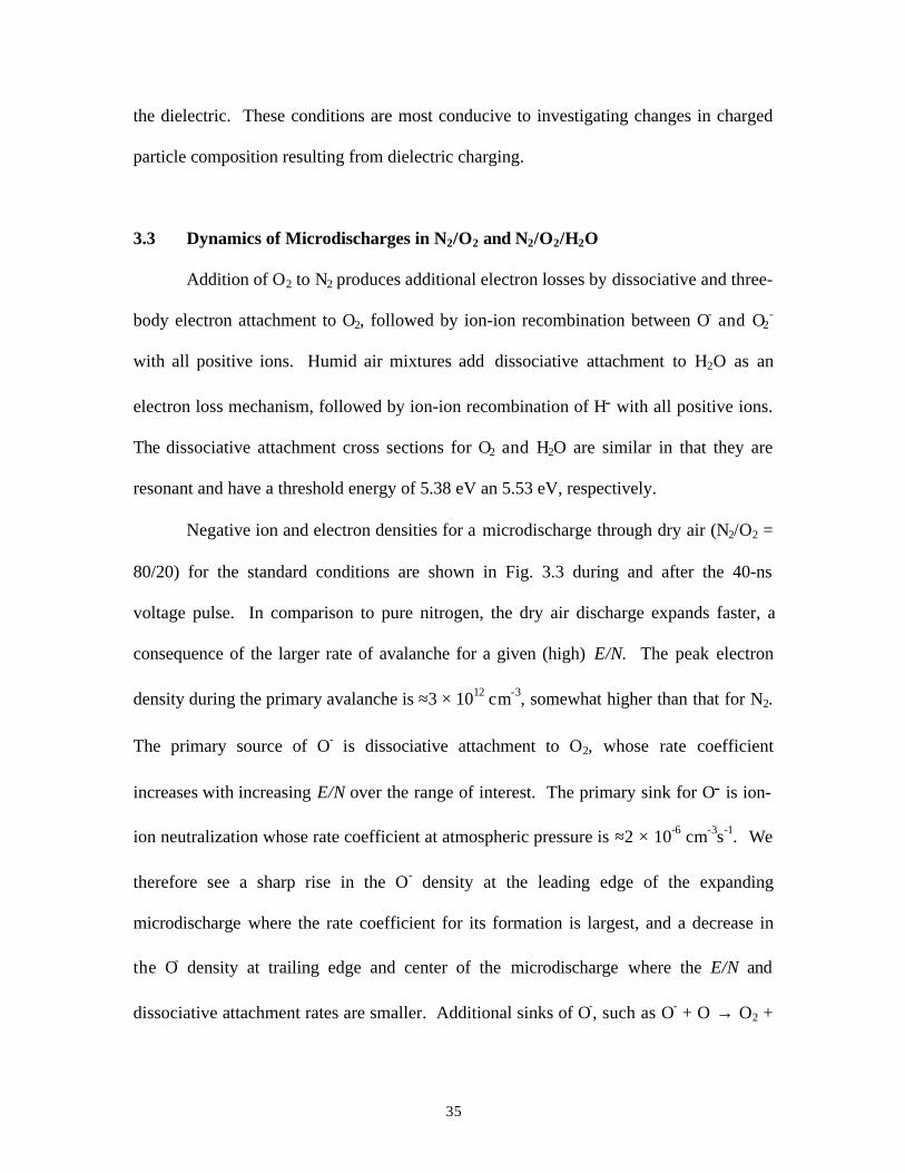
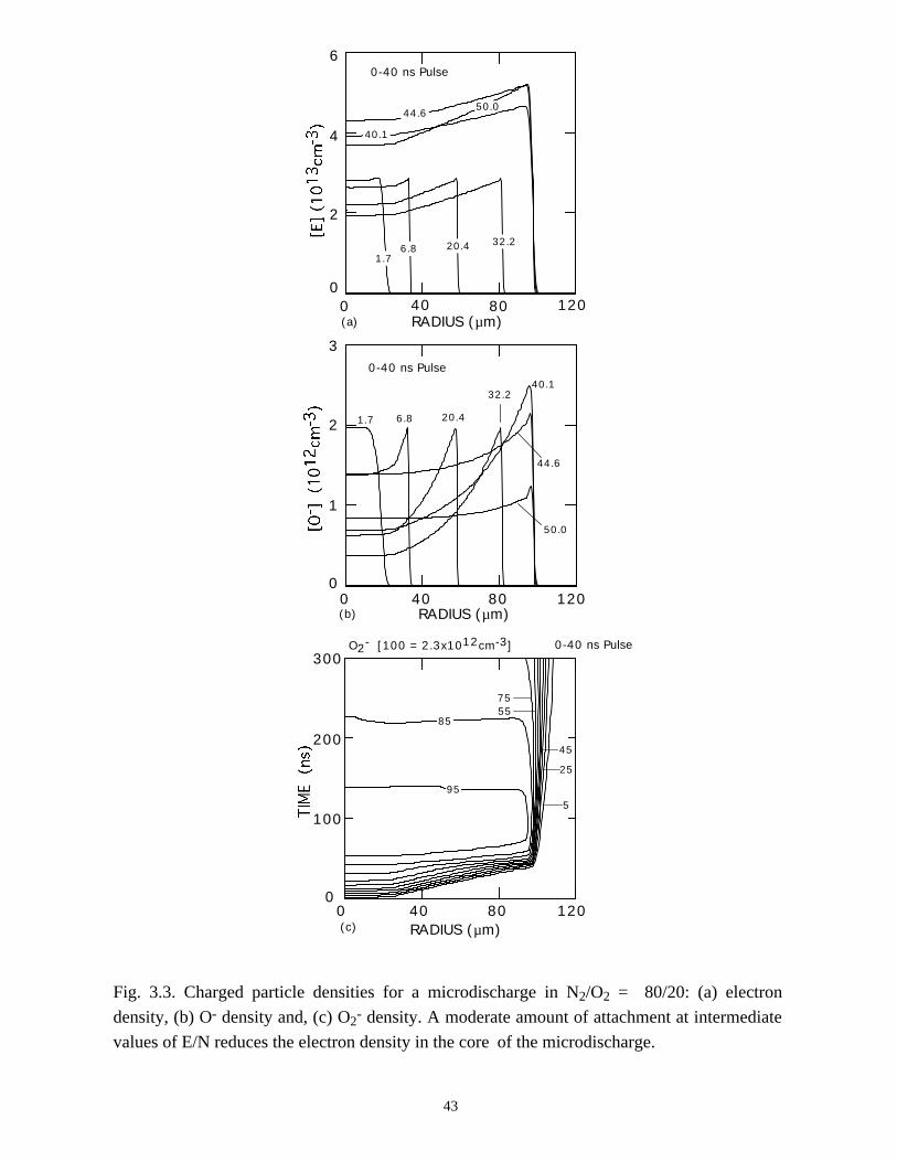
Negative ion and electron densities for a microdischarge through dry air (N2/O2 =
80/20) for the standard conditions are shown in Fig. 3.3 during and after the 40-ns
voltage pulse. In comparison to pure nitrogen, the dry air discharge expands faster, a
consequence of the larger rate of avalanche for a given (high) E/N. The peak electron
density during the primary avalanche is ≈3 × 1012 cm-3, somewhat higher than that for N2.
The primary source of O- is dissociative attachment to O2, whose rate coefficient
increases with increasing E/N over the range of interest. The primary sink for O- is ion-
ion neutralization whose rate coefficient at atmospheric pressure is ≈2 × 10⁻⁶ cm-3s-1. We
therefore see a sharp rise in the O- density at the leading edge of the expanding
microdischarge where the rate coefficient for its formation is largest, and a decrease in
the O- density at trailing edge and center of the microdischarge where the E/N and
dissociative attachment rates are smaller. Additional sinks of O-, such as O- + O → O2 +
36
e, also contribute to reducing the O- density in the center of the microdischarge. The
electron density also decreases in the center of the microdischarge, though at a lower rate
due to its lower rate of electron-ion recombination and due to the presence of a source of
electrons from O- detachment. The density of O2- does not exhibit a peak at the leading
edge of the expanding microdischarge because the rate coefficient for 3-body attachment
decreases with increasing E/N and will, in fact, increase after the voltage collapses in the
gap.
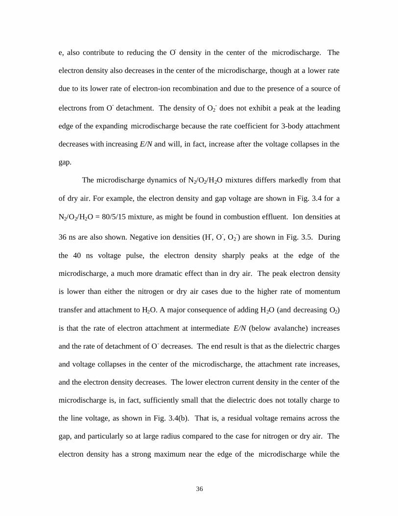
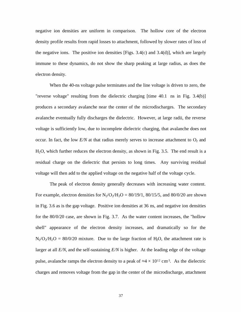
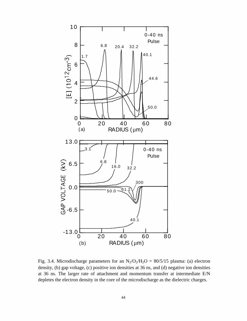
The microdischarge dynamics of N2/O2/H2O mixtures differs markedly from that
of dry air. For example, the electron density and gap voltage are shown in Fig. 3.4 for a
N2/O2/H2O = 80/5/15 mixture, as might be found in combustion effluent. Ion densities at
36 ns are also shown. Negative ion densities (H-, O-, O2-) are shown in Fig. 3.5. During
the 40 ns voltage pulse, the electron density sharply peaks at the edge of the
microdischarge, a much more dramatic effect than in dry air. The peak electron density
is lower than either the nitrogen or dry air cases due to the higher rate of momentum
transfer and attachment to H2O. A major consequence of adding H2O (and decreasing O2)
is that the rate of electron attachment at intermediate E/N (below avalanche) increases
and the rate of detachment of O- decreases. The end result is that as the dielectric charges
and voltage collapses in the center of the microdischarge, the attachment rate increases,
and the electron density decreases. The lower electron current density in the center of the
microdischarge is, in fact, sufficiently small that the dielectric does not totally charge to
the line voltage, as shown in Fig. 3.4(b). That is, a residual voltage remains across the
gap, and particularly so at large radius compared to the case for nitrogen or dry air. The
electron density has a strong maximum near the edge of the microdischarge while the
37
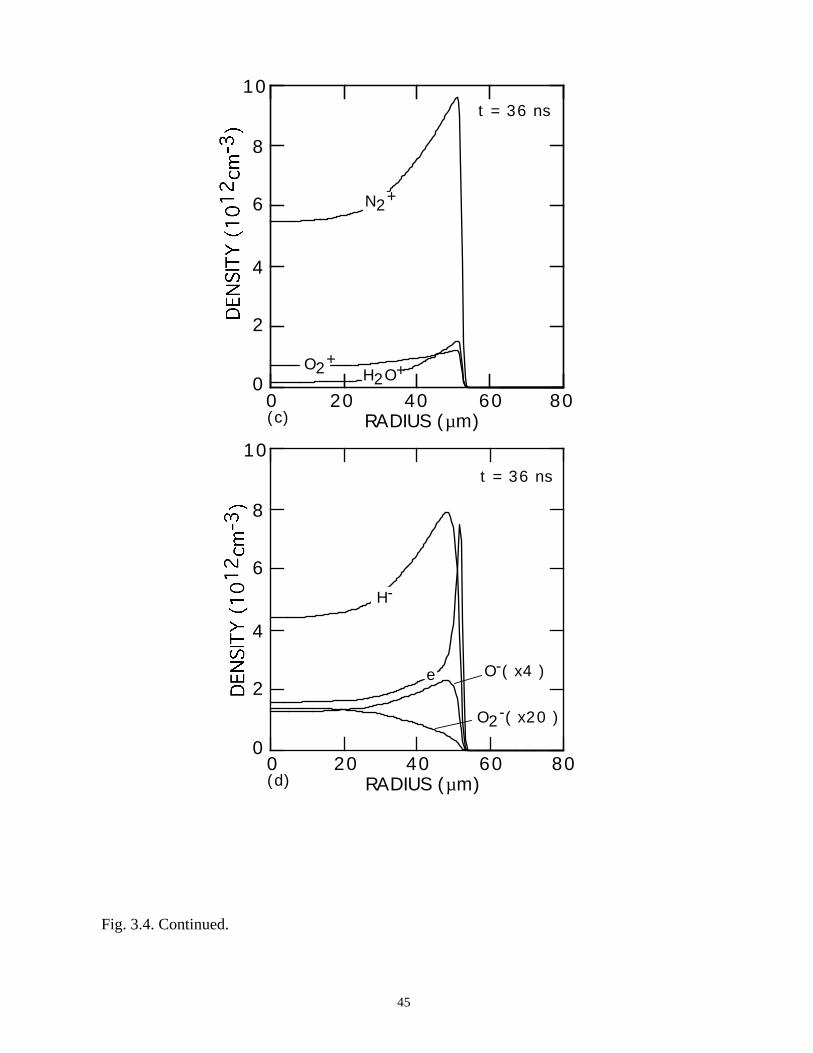
negative ion densities are uniform in comparison. The hollow core of the electron
density profile results from rapid losses to attachment, followed by slower rates of loss of
the negative ions. The positive ion densities [Figs. 3.4(c) and 3.4(d)], which are largely
immune to these dynamics, do not show the sharp peaking at large radius, as does the
electron density.
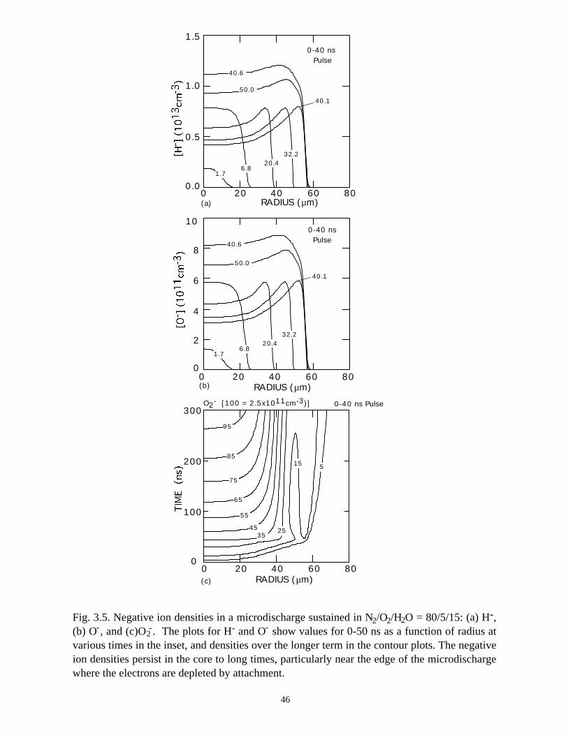
When the 40-ns voltage pulse terminates and the line voltage is driven to zero, the
"reverse voltage" resulting from the dielectric charging [time 40.1 ns in Fig. 3.4(b)]
produces a secondary avalanche near the center of the microdischarges. The secondary
avalanche eventually fully discharges the dielectric. However, at large radii, the reverse
voltage is sufficiently low, due to incomplete dielectric charging, that avalanche does not
occur. In fact, the low E/N at that radius merely serves to increase attachment to O2 and
H2O, which further reduces the electron density, as shown in Fig. 3.5. The end result is a
residual charge on the dielectric that persists to long times. Any surviving residual
voltage will then add to the applied voltage on the negative half of the voltage cycle.
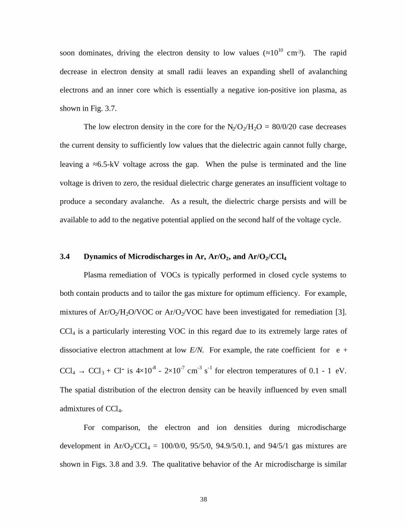
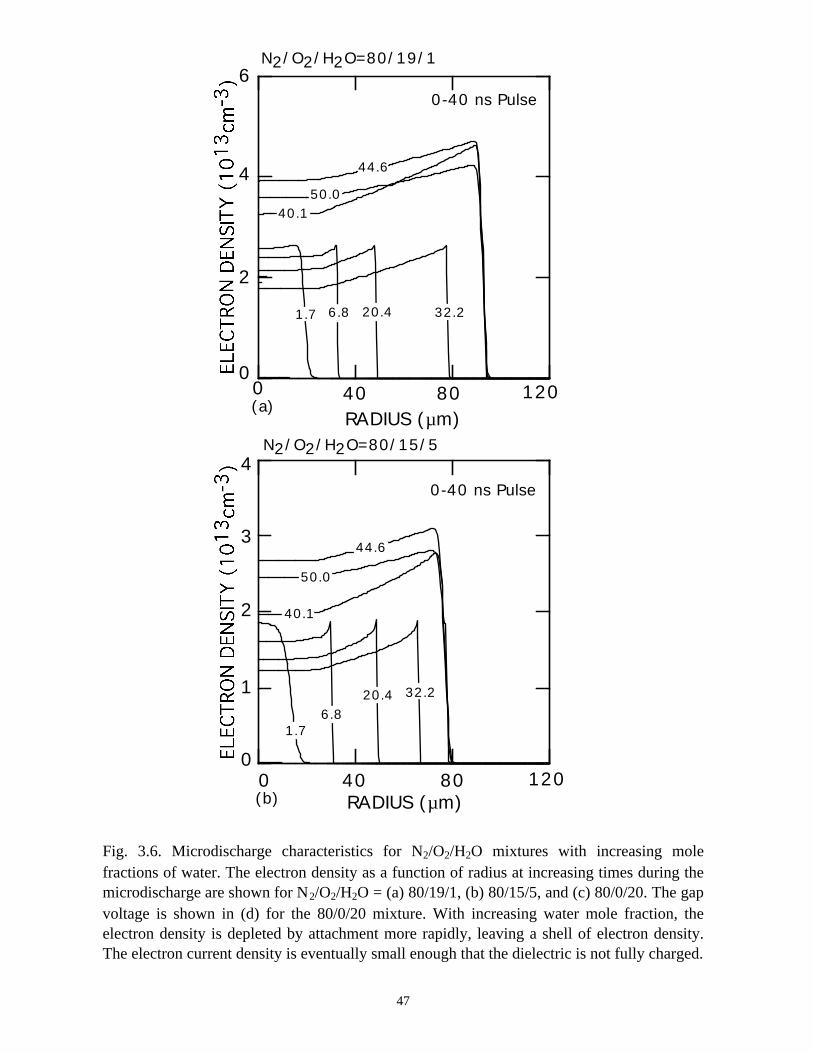
The peak of electron density generally decreases with increasing water content.
For example, electron densities for N2/O2/H2O = 80/19/1, 80/15/5, and 80/0/20 are shown
in Fig. 3.6 as is the gap voltage. Positive ion densities at 36 ns, and negative ion densities
for the 80/0/20 case, are shown in Fig. 3.7. As the water content increases, the "hollow
shell" appearance of the electron density increases, and dramatically so for the
N2/O2/H2O = 80/0/20 mixture. Due to the large fraction of H2O, the attachment rate is
larger at all E/N, and the self-sustaining E/N is higher. At the leading edge of the voltage
pulse, avalanche ramps the electron density to a peak of ≈4 × 1012 cm-3. As the dielectric
charges and removes voltage from the gap in the center of the microdischarge, attachment
38
soon dominates, driving the electron density to low values (≈1010 cm-3). The rapid
decrease in electron density at small radii leaves an expanding shell of avalanching
electrons and an inner core which is essentially a negative ion-positive ion plasma, as
shown in Fig. 3.7.
The low electron density in the core for the N2/O2/H2O = 80/0/20 case decreases
the current density to sufficiently low values that the dielectric again cannot fully charge,
leaving a ≈6.5-kV voltage across the gap. When the pulse is terminated and the line
voltage is driven to zero, the residual dielectric charge generates an insufficient voltage to
produce a secondary avalanche. As a result, the dielectric charge persists and will be
available to add to the negative potential applied on the second half of the voltage cycle.
3.4 Dynamics of Microdischarges in Ar, Ar/O2, and Ar/O2/CCl4
Plasma remediation of VOCs is typically performed in closed cycle systems to
both contain products and to tailor the gas mixture for optimum efficiency. For example,
mixtures of Ar/O2/H2O/VOC or Ar/O2/VOC have been investigated for remediation [3].
CCl4 is a particularly interesting VOC in this regard due to its extremely large rates of
dissociative electron attachment at low E/N. For example, the rate coefficient for e +
CCl4 → CCl3 + Cl- is 4×10⁻⁸ - 2×10⁻⁷ cm-3 s-1 for electron temperatures of 0.1 - 1 eV.
The spatial distribution of the electron density can be heavily influenced by even small
admixtures of CCl4.
For comparison, the electron and ion densities during microdischarge
development in Ar/O2/CCl4 = 100/0/0, 95/5/0, 94.9/5/0.1, and 94/5/1 gas mixtures are
shown in Figs. 3.8 and 3.9. The qualitative behavior of the Ar microdischarge is similar
39
to that of the N2 discharge. The microdischarge expands radially, fully charging the
dielectric leaving behind a positive ion-electron plasma which slowly recombines. A
secondary discharge raises the electron and ion density across the entire "preionized"
radius when the line voltage is pulled to zero. The addition of 5% O2 does not
appreciably change the electron profiles other than reducing the density in the low E/N
core due to attachment.
With the addition of 0.1% CCl4 (Ar/O2/CCl4 = 94.9/5/0.1) there is a large increase
in the attachment rate at low E/N. As the dielectric charges, thereby lowering E/N in the
center of the microdischarge, attachment dominates, leaving behind an expanding
avalanching shell of electrons, and a core that is largely composed of negative and
positive ions. This effect is heightened by increasing the CCl4 fraction to 1%
(Ar/O2/CCl4 = 94/5/1). Here the higher attachment rate in the core consumes the
electrons within a few ns of the local E/N falling below self sustaining, leaving behind a
thin electron shell. The charged particle core of the microdischarge is composed almost
exclusively of CCl3+ and Cl-. The secondary avalanche generates more uniform electron
distribution within the streamer due to “preionization.”
3.5 Concluding Remarks
Microdischarge dynamics in dielectric barrier discharges have been investigated
for gas mixtures with varying degrees of electronegativity. We found that in
electropositive mixtures, the expanding microdischarge retains a fairly uniform electron
density as a function of radius, suffering a small reduction in the core of the
microdischarge due to electron-ion recombination. Dielectric charging and the reduction
40
of E/N at small radius has little effect on recombination rates. However in
electronegative gas mixtures, particularly those whose attachment rate increases with
decreasing E/N, the core of the microdischarge may quickly evolve to a negative ion-
positive ion plasma. The effect is particularly acute in thermal attaching gas mixtures
such as those containing CCl4. Microdischarge expansion will, in the absence of
dielectric charging at radii ahead of the core, proceed unimpeded as long as voltage is
available. The stalling of the expansion is attributed to transverse components of the
electric field on or near the dielectric which charges the dielectric ahead of the body of
the microdischarge.
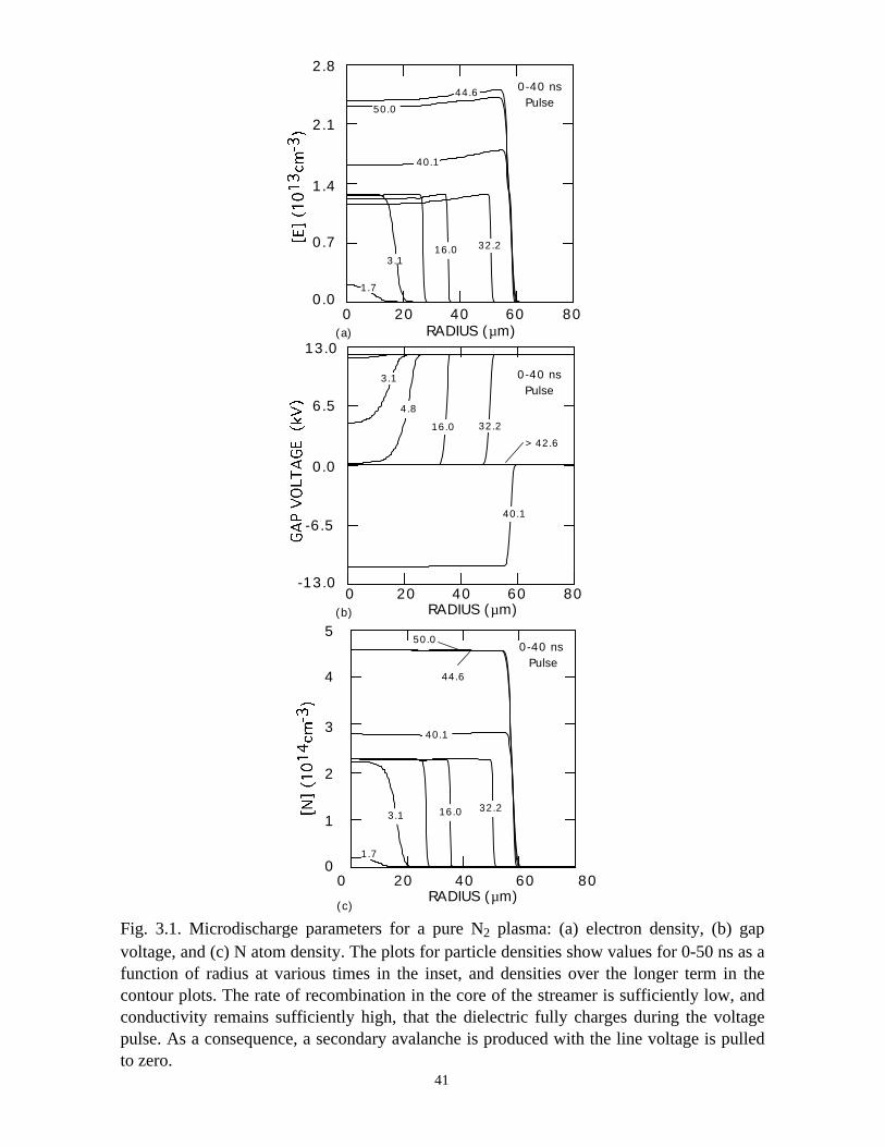
Fig. 3.1. Microdischarge parameters for a pure N2 plasma: (a) electron density, (b) gapvoltage, and (c) N atom density. The plots for particle densities show values for 0-50 ns as afunction of radius at various times in the inset, and densities over the longer term in thecontour plots. The rate of recombination in the core of the streamer is sufficiently low, andconductivity remains sufficiently high, that the dielectric fully charges during the voltagepulse. As a consequence, a secondary avalanche is produced with the line voltage is pulledto zero.
41
(b)806040200
RADIUS (µm)
-6.5
0.0
6.5
-13.0
13.0
0-40 nsPulse
40.1
4.8
16.0
> 42.6
3.1
32.2
0.0
2.1
0.7
1.4
2.8
(a)806040200
RADIUS (µm)
0-40 nsPulse
44.6
50.0
32.216.0
1.7
40.1
3.1
(c)
0
3
1
2
5
4
806040200RADIUS (µm)
0-40 ns Pulse
44.6
1.7
3.1 16.0 32.2
40.1
50.0
0
20
40
60
80
100
120
0 10 20 30 40 50 60TIME (ns)
15 kV0-40 ns Pulse
(a)
0 10 20 30 40 50 60TIME (ns)
0
10
20
30
40
50
600-40 ns Pulse
12 kV
(b)
14 kV
13 kV
12 kV
11 kV
ρ = 700 MΩ/
ρ =
Fig. 3.2. Radius of the microdischarge in N2 (a) as a function of line voltage and (b)with/without surface conductivity. In the absence of a mechanism to reduce gap voltageahead of the body of the microdischarge, the microdischarge continues to expand as longas voltage is applied. A small surface conductivity bleeds charge to larger radii, therebyreducing the gap voltage and halting expansion.
42
0-40 ns Pulse
85
595
5575
45
25
(c) RADIUS (µm)12080400
100
200
300
0
O2- [100 = 2.3x1012cm-3]
RADIUS (µm)12080400
(b)
0
1
3
2
0-40 ns Pulse40.1
32.2
6.8 20.41.7
44.6
50.0
RADIUS (µm)12080400
(a)
0
2
6
4
0-40 ns Pulse
1.76.8 20.4 32.2
40.1
44.650.0
Fig. 3.3. Charged particle densities for a microdischarge in N2/O2 = 80/20: (a) electron
density, (b) O- density and, (c) O2- density. A moderate amount of attachment at intermediate
values of E/N reduces the electron density in the core of the microdischarge.
43
806040200
0-40 nsPulse
50.0
6.816.0 32.2
3.1
61.2
300
RADIUS (µm)
40.1
(b)
0.0
6.5
13.0
-13.0
-6.5
806040200(a) RADIUS (µm)
0
6
2
4
10
8
0-40 nsPulse
40.1
44.6
50.0
32.26.8 20.4
1.7
Fig. 3.4. Microdischarge parameters for an N2/O2/H2O = 80/5/15 plasma: (a) electrondensity, (b) gap voltage, (c) positive ion densities at 36 ns, and (d) negative ion densitiesat 36 ns. The larger rate of attachment and momentum transfer at intermediate E/Ndepletes the electron density in the core of the microdischarge as the dielectric charges.
44
806040200(c) RADIUS (µm)
t = 36 ns
0
2
4
6
8
10
N2+
O2+H2O+
806040200(d) RADIUS (µm)
t = 36 ns
0
2
4
6
8
10
O2-( x20 )
H-
O-( x4 )e
Fig. 3.4. Continued.
45
O2- [100 = 2.5x1011cm-3)]
806040200
100
200
300
0
RADIUS (µm)
515
2535
45
55
65
75
85
95
(c)
0-40 ns Pulse
(a)806040200
RADIUS (µm)
0-40 ns Pulse
0.0
0.5
1.5
1.040.1
1.76.8
20.432.2
40.6
50.0
(b)806040200
RADIUS (µm)
0
6
2
4
10
8
0-40 nsPulse
40.1
1.76.8
20.432.2
40.6
50.0
Fig. 3.5. Negative ion densities in a microdischarge sustained in N /O /H O = 80/5/15: (a) H-,(b) O , and (c)O . The plots for H and O show values for 0-50 ns as a function of radius atvarious times in the inset, and densities over the longer term in the contour plots. The negativeion densities persist in the core to long times, particularly near the edge of the microdischargewhere the electrons are depleted by attachment.
46
2 2 2-- -
2-
N2/O2/H2O=80/19/1
(a)8040 1200
RADIUS (µm)
0
2
4
60-40 ns Pulse
40.150.0
44.6
20.41.7 32.26.8
6.8
0-40 ns Pulse
N2/O2/H2O=80/15/5
8040 1200RADIUS (µm)
0
2
1
4
3
1.7
40.1
32.220.4
44.6
50.0
(b)
Fig. 3.6. Microdischarge characteristics for N2/O2/H2O mixtures with increasing molefractions of water. The electron density as a function of radius at increasing times during themicrodischarge are shown for N2/O2/H2O = (a) 80/19/1, (b) 80/15/5, and (c) 80/0/20. The gapvoltage is shown in (d) for the 80/0/20 mixture. With increasing water mole fraction, theelectron density is depleted by attachment more rapidly, leaving a shell of electron density.The electron current density is eventually small enough that the dielectric is not fully charged.
47
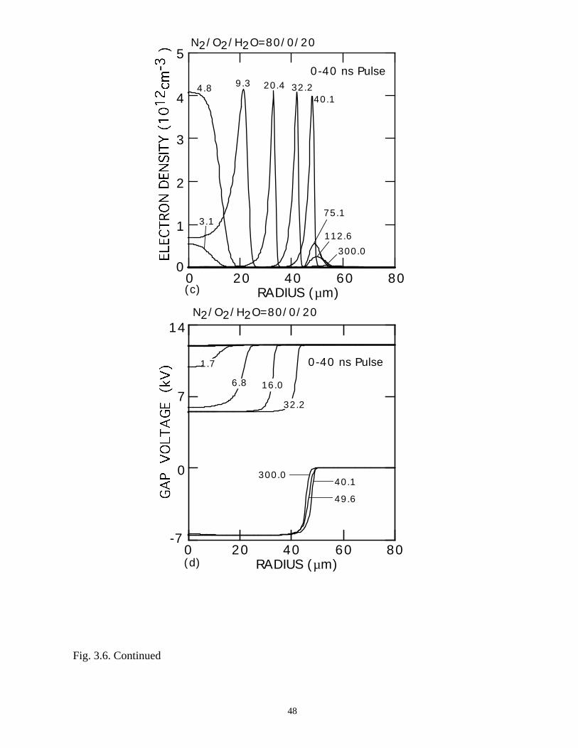
40.132.220.4
3.1
4.8 9.3
75.1
112.6
300.0
806040200RADIUS (µm)
1
2
3
4
5
0
(c)
0-40 ns Pulse
N2/O2/H2O=80/0/20
(d)
-7
0
7
14
40.1
6.8
32.2
300.0
0-40 ns Pulse1.7
49.6
806040200RADIUS (µm)
N2/O2/H2O=80/0/20
16.0
Fig. 3.6. Continued
48
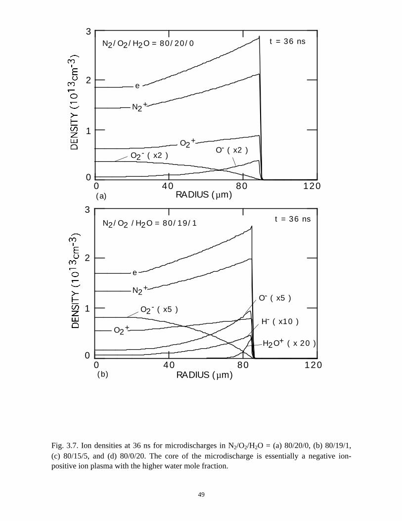
0
2
1
3
(a)
O2- ( x2 )O- ( x2 )
12080400RADIUS (µm)
t = 36 nsN2/O2/H2O = 80/20/0
N2+
e
O2+
(b)
O2- ( x5 )O- ( x5 )
12080400RADIUS (µm)
0
2
1
3t = 36 ns
H2O+ ( x 20 )
H- ( x10 )
N2/O2 /H2O = 80/19/1
e
N2+
O2+
Fig. 3.7. Ion densities at 36 ns for microdischarges in N2/O2/H2O = (a) 80/20/0, (b) 80/19/1,(c) 80/15/5, and (d) 80/0/20. The core of the microdischarge is essentially a negative ion-positive ion plasma with the higher water mole fraction.
49
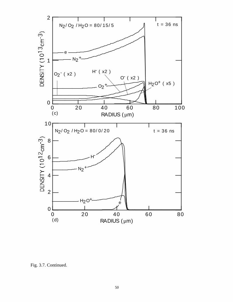
(c)
H2O+ ( x5 )O- ( x2 )
RADIUS (µm)
t = 36 ns
H- ( x2 )O2- ( x2 )
N2/O2 /H2O = 80/15/5
0
2
1
806040200 100
eN2+
O2+
806040200(d) RADIUS (µm)
t = 36 ns
0
2
4
6
8
10
H-
N2+
H2O+e
N2/O2 /H2O = 80/0/20
Fig. 3.7. Continued.
50
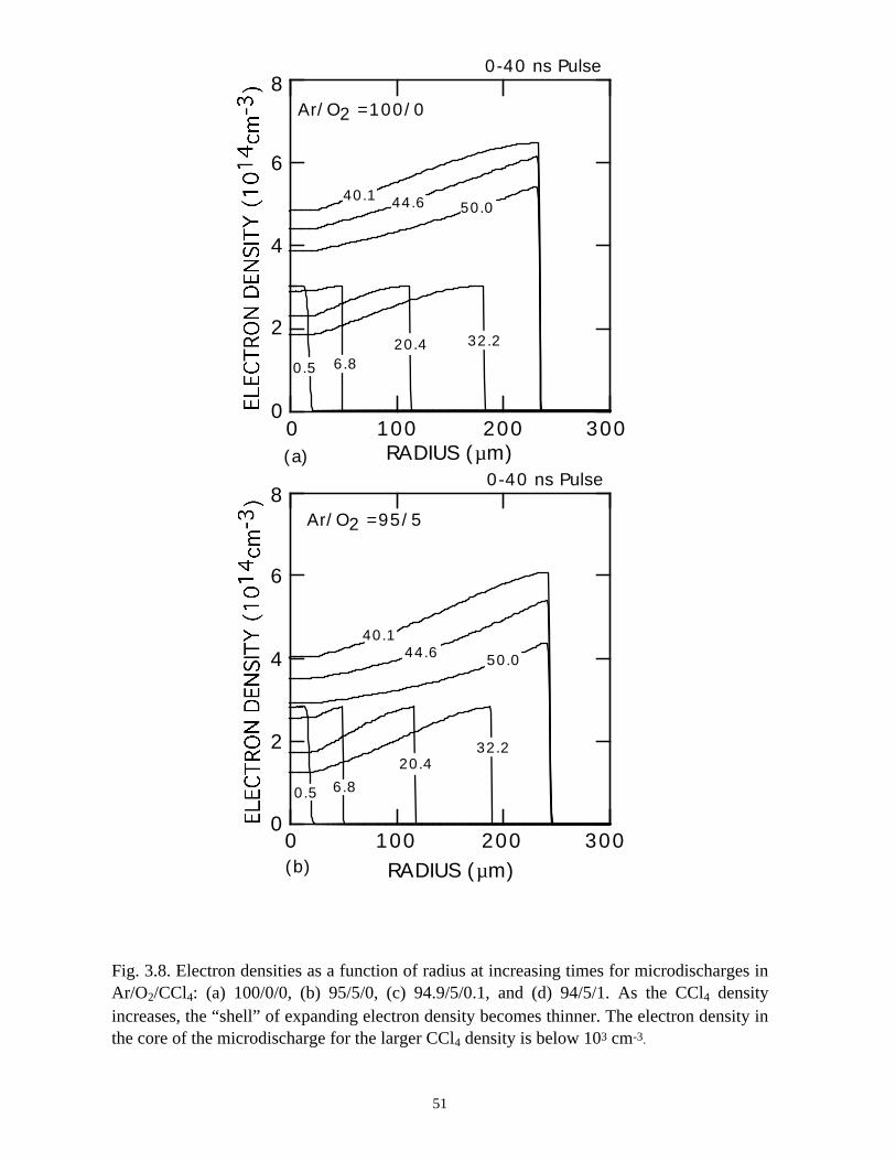
0-40 ns Pulse
0 100 200 300(b)
Ar/O2 =95/5
RADIUS (µm)
4
0
2
6
8
50.0
40.144.6
32.2
0.5
20.4
6.8
RADIUS (µm)(a)0 100 200 300
4
0
2
6
80-40 ns Pulse
50.040.1
Ar/O2 =100/0
44.6
32.220.4
0.5 6.8
Fig. 3.8. Electron densities as a function of radius at increasing times for microdischarges inAr/O2/CCl4: (a) 100/0/0, (b) 95/5/0, (c) 94.9/5/0.1, and (d) 94/5/1. As the CCl4 densityincreases, the “shell” of expanding electron density becomes thinner. The electron density inthe core of the microdischarge for the larger CCl4 density is below 103 cm-3.
51
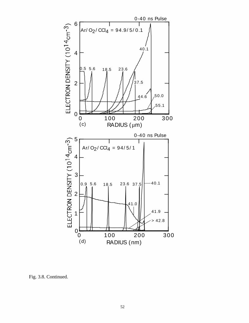
0-40 ns Pulse
1
2
3
4
5
03002001000
RADIUS (nm)(d)
40.1
Ar/O2/CCl4 = 94/5/1
0.9 5.6 18.5 23.6 37.5
41.0
41.9
> 42.8
0-40 ns Pulse
0.5 5.6 18.5 23.6
50.0
55.1
30020010000
2
4
6Ar/O2/CCl4 = 94.9/5/0.1
(c) RADIUS (µm)
44.6
37.5
40.1
Fig. 3.8. Continued.
52
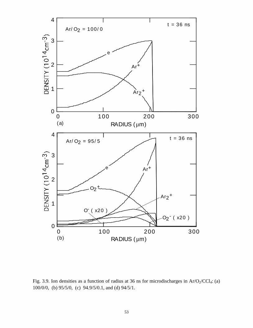
RADIUS (µm)
Ar/O2 = 95/5
(b)
Ar2+
O- ( x20 )
30020010000
2
4
1
3
t = 36 ns
e Ar+
O2+
O2- ( x20 )
(a)3002001000
RADIUS (µm)
0
2
4
1
3
t = 36 ns
e
Ar+
Ar2+
Ar/O2 = 100/0
Fig. 3.9. Ion densities as a function of radius at 36 ns for microdischarges in Ar/O2/CCl4: (a)100/0/0, (b) 95/5/0, (c) 94.9/5/0.1, and (d) 94/5/1.
53
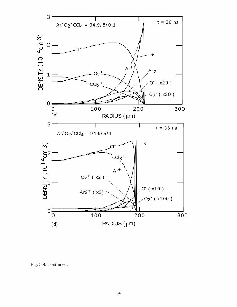
RADIUS (µm)(c)
e
Ar2+
O- ( x20 )
30020010000
2
1
3Ar/O2/CCl4 = 94.9/5/0.1 t = 36 ns
Cl-
Ar+O2+
CCl3+
O2- ( x20 )
(d)
Ar2+ ( x2)
e
O2+ ( x2 )Ar+
3002001000RADIUS (µm)
0
2
1
3t = 36 ns
Ar/O2/CCl4 = 94.9/5/1
Cl-
CCl3+
O- ( x10 )
O2- ( x100 )
Fig. 3.9. Continued.
54
55
3.6 References
[1] B. Eliasson and U. Kogelschatz, IEEE Trans. Plasma Sci. 19, 309 (1991).
[2] A. C. Gentile and M. J. Kushner, J. Appl. Phys. 79, 3877 (1996).
[3] L. A. Rosocha, G. K. Anderson, L. A. Bechtold, J. J. Coogan, H. G. Hech, M.
Kang, W. H. McCulla, R. A. Tennant, and P. J. Wantuck, in Nonthermal Plasma
Techniques for Pollution Control, edited by B. N. Penetrante and S. E. Schultheis
(Springer, Berlin, 1993), Part B, pp. 281.
56
4. MULTIPLE MICRODISCHARGE DYNAMICS IN DIELECTRICBARRIER DISCHARGES
4.1 Introduction
In the last chapter, we addressed the radially symmetric dynamics of a single
microdischarge. In this chapter, we report on results from a 2-D PCHM modeling study
in which we address the complementary problem of the expansion of multiple, and hence
radially asymmetric, microdischarges in close vicinity. We will investigate N2 and dry
air (N2/O2) discharges as examples of nonattaching and attaching discharges. The
microdischarge development for 1-4 adjacent microdischarges in N2 is presented in
Section 4.2. In Section 4.3, we examine the dynamics of two closely space
microdischarges in N2/O2. In Section 4.4, we discuss the consequences of remnant
surface charges on microdischarge spreading. Our concluding remarks are in Section 4.5.
4.2 Multi-Microdischarges Dynamics in N2
We begin our discussion of multi-microdischarge dynamics in DBDs by
examining two microdischarges in pure N2. Initial conditions are generated by specifying
(or randomly distributing) a center point for each microdischarge in the 2-D domain. The
microdischarge is assumed to be initially radially symmetric and composed of a seed
electron density having a super-Gaussian profile with peak density of n0 = 109 cm-3 and
radius r0 = 15 µm. Initial electron densities that would be smaller than 10-4 n0 are set
equal to zero. The pressure is one atmosphere at 400 K. One electrode is covered by 0.5-
mm thickness of a dielectric having permittivity of 25ε0 with 0.25-cm gas gap. The
57
applied voltage is a square pulse of specified duration and magnitude unless stated
otherwise.
The electron density is shown in Fig. 4.1 for two microdischarges in N2 separated
by 300 µm for a square wave 40-ns voltage pulse of 12 kV. Results are shown for times
of 0.8, 26, 41 and 100 ns. One-dimensional slices of the electron density through the axis
of symmetry are shown in Fig. 4.2. Only the upper half of the microdischarges are
shown in Fig. 4.1, taking advantage of symmetry across the lower horizontal axis. As in
Chapter 3, we have chosen conditions for which the microdischarge will continue to
expand for the duration of the voltage pulse in order to reduce the importance of issues
related to surface conductivity of the substrate. The expanding microdischarges retain
their initial circular profiles until they collide. Note the somewhat hollow appearance of
the microdischarges. As in the case of the single microdischarge, charging of the
dielectric in the center of the microdischarge produces a collapse of the E/N in the bulk
plasma, which reduces the rate of electron generating collisions (e.g., ionization) and
increases the rate of electron consuming collisions, in this case dissociative
recombination. At 40 ns when the voltage is pulled to zero, the electric field resulting
from charging the dielectric produces a secondary discharge in a manner similar to that
for the single discharge. Further expansion does not occur during the secondary
avalanche since the dielectric outside the microdischarge is not charged.
When the microdischarges collide, a peak in the electron density occurs at the
interface, having an enhancement of ≈13% over the single microdischarge. This increase
can be attributed to two causes. The first, in a sense, is a consequence of the initial
conditions. Electrons from the microdischarge diffuse into regions of uncharged
58
dielectric, followed by avalanche that begins charging the dielectric. The peak electron
density occurs as the voltage across the gap falls below the self-sustaining value and net
electron generation turns negative. The peak electron density therefore weakly depends
on the initial electron density since there is some dynamic “overshoot” of the equilibrium
conditions. Since we have contributions from expansion by both microdischarges to the
effective n0 at the interface, the initial electron density for avalanche at that location is
larger. As a consequence the maximum electron density is larger. The second effect is
hydrodynamic in nature. The ions and neutrals can, from a hydrodynamic standpoint, be
considered well coupled fluids. The inertia of the expanding plasma column results in
the shells of the colliding microdischarges producing a higher gas density. Since the ions
are entrained in this flow, the ion density increases commensurably.
The plasma expansion of the microdischarges terminates on the sides where the
collision occurs, but continues to expand on the opposite sides. The end result is an
elongated appearance to the microdischarges. The microdischarges do not “pass
through” each other as would, for example, expanding acoustic waves. Recall that the
expansion of the microdischarges is sustained by diffusion of electrons into regions in
which the dielectric is uncharged, thereby enabling avalanche and growth of the
microdischarge. Since at the interface, electron diffusion occurs into regions in which the
dielectric is already charged, further avalanche and expansion does not occur.
The gas temperature in the microdischarge depends on the total energy deposition,
manner of dissipation of deposited energy and change in enthalpy due to chemical
reactions and radiative decay of excited states. Gradients in temperature also produce a
pressure gradient which can lead to advection. For example, 1-D slices of the gas
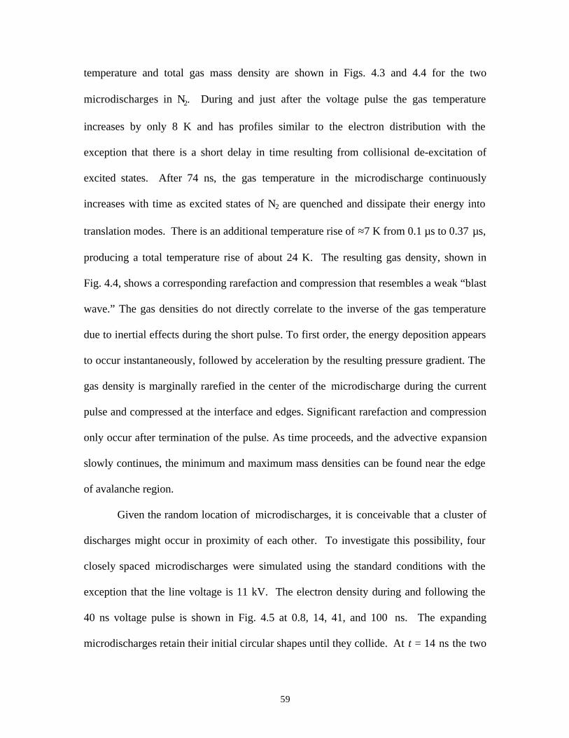
59
temperature and total gas mass density are shown in Figs. 4.3 and 4.4 for the two
microdischarges in N2. During and just after the voltage pulse the gas temperature
increases by only 8 K and has profiles similar to the electron distribution with the
exception that there is a short delay in time resulting from collisional de-excitation of
excited states. After 74 ns, the gas temperature in the microdischarge continuously
increases with time as excited states of N2 are quenched and dissipate their energy into
translation modes. There is an additional temperature rise of ≈7 K from 0.1 µs to 0.37 µs,
producing a total temperature rise of about 24 K. The resulting gas density, shown in
Fig. 4.4, shows a corresponding rarefaction and compression that resembles a weak “blast
wave.” The gas densities do not directly correlate to the inverse of the gas temperature
due to inertial effects during the short pulse. To first order, the energy deposition appears
to occur instantaneously, followed by acceleration by the resulting pressure gradient. The
gas density is marginally rarefied in the center of the microdischarge during the current
pulse and compressed at the interface and edges. Significant rarefaction and compression
only occur after termination of the pulse. As time proceeds, and the advective expansion
slowly continues, the minimum and maximum mass densities can be found near the edge
of avalanche region.
Given the random location of microdischarges, it is conceivable that a cluster of
discharges might occur in proximity of each other. To investigate this possibility, four
closely spaced microdischarges were simulated using the standard conditions with the
exception that the line voltage is 11 kV. The electron density during and following the
40 ns voltage pulse is shown in Fig. 4.5 at 0.8, 14, 41, and 100 ns. The expanding
microdischarges retain their initial circular shapes until they collide. At t = 14 ns the two
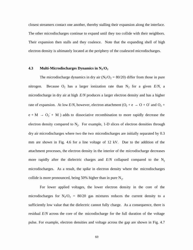
60
closest streamers contact one another, thereby stalling their expansion along the interface.
The other microdischarges continue to expand until they too collide with their neighbors.
Their expansion then stalls and they coalesce. Note that the expanding shell of high
electron density is ultimately located at the periphery of the coalesced microdischarges.
4.3 Multi-Microdischarges Dynamics in N2/O2
The microdischarge dynamics in dry air (N2/O2 = 80/20) differ from those in pure
nitrogen. Because O2 has a larger ionization rate than N2 for a given E/N, a
microdischarge in dry air at high E/N produces a larger electron density and has a higher
rate of expansion. At low E/N, however, electron attachment (O2 + e → O + O- and O2 +
e + M → O2- + M ) adds to dissociative recombination to more rapidly decrease the
electron density compared to N2. For example, 1-D slices of electron densities through
dry air microdischarges where two the two microdischarges are initially separated by 0.3
mm are shown in Fig. 4.6 for a line voltage of 12 kV. Due to the addition of the
attachment processes, the electron density in the interior of the microdischarge decreases
more rapidly after the dielectric charges and E/N collapsed compared to the N2
microdischarges. As a result, the spike in electron density where the microdischarges
collide is more pronounced, being 50% higher than in pure N2.
For lower applied voltages, the lower electron density in the core of the
microdischarges for N2/O2 = 80/20 gas mixtures reduces the current density to a
sufficiently low value that the dielectric cannot fully charge. As a consequence, there is
residual E/N across the core of the microdischarge for the full duration of the voltage
pulse. For example, electron densities and voltage across the gap are shown in Fig. 4.7
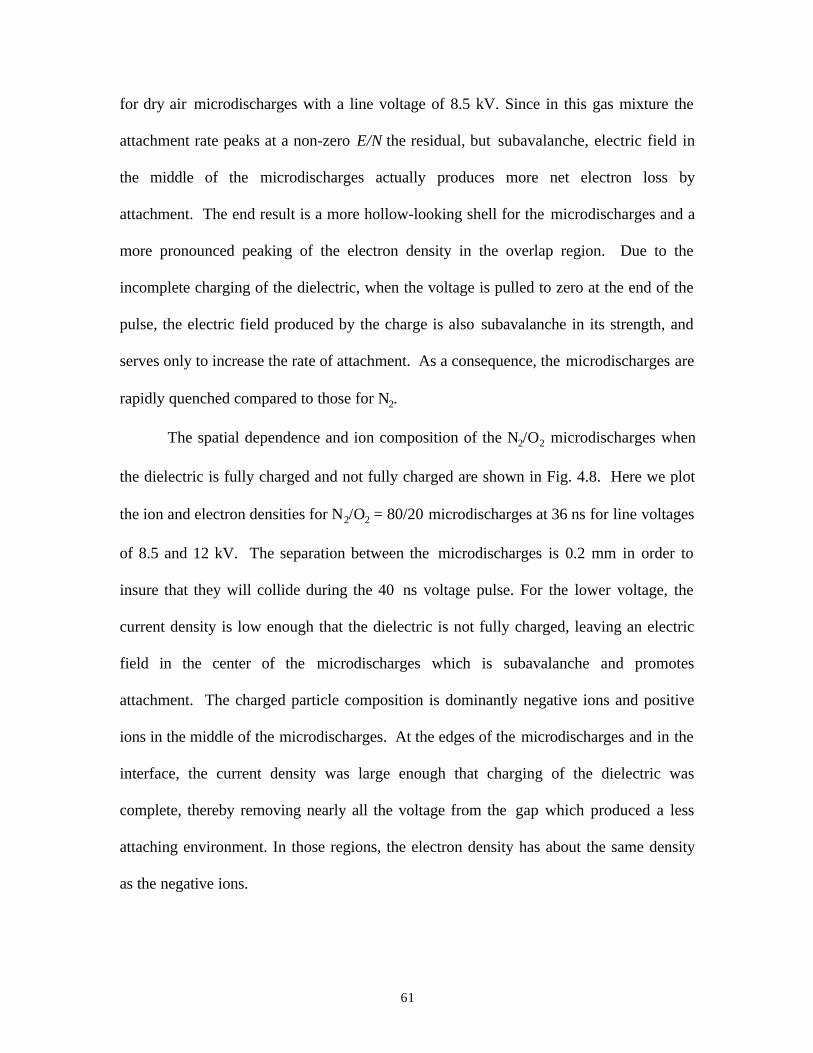
61
for dry air microdischarges with a line voltage of 8.5 kV. Since in this gas mixture the
attachment rate peaks at a non-zero E/N the residual, but subavalanche, electric field in
the middle of the microdischarges actually produces more net electron loss by
attachment. The end result is a more hollow-looking shell for the microdischarges and a
more pronounced peaking of the electron density in the overlap region. Due to the
incomplete charging of the dielectric, when the voltage is pulled to zero at the end of the
pulse, the electric field produced by the charge is also subavalanche in its strength, and
serves only to increase the rate of attachment. As a consequence, the microdischarges are
rapidly quenched compared to those for N2.
The spatial dependence and ion composition of the N2/O2 microdischarges when
the dielectric is fully charged and not fully charged are shown in Fig. 4.8. Here we plot
the ion and electron densities for N2/O2 = 80/20 microdischarges at 36 ns for line voltages
of 8.5 and 12 kV. The separation between the microdischarges is 0.2 mm in order to
insure that they will collide during the 40 ns voltage pulse. For the lower voltage, the
current density is low enough that the dielectric is not fully charged, leaving an electric
field in the center of the microdischarges which is subavalanche and promotes
attachment. The charged particle composition is dominantly negative ions and positive
ions in the middle of the microdischarges. At the edges of the microdischarges and in the
interface, the current density was large enough that charging of the dielectric was
complete, thereby removing nearly all the voltage from the gap which produced a less
attaching environment. In those regions, the electron density has about the same density
as the negative ions.
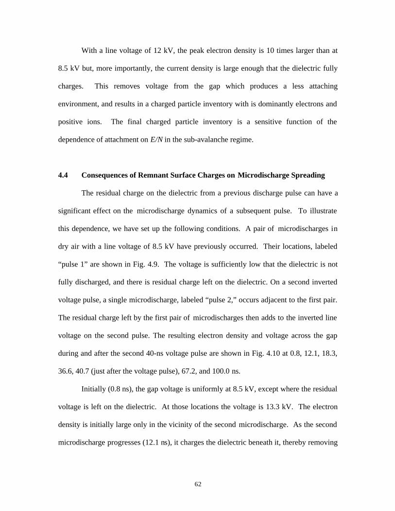
62
With a line voltage of 12 kV, the peak electron density is 10 times larger than at
8.5 kV but, more importantly, the current density is large enough that the dielectric fully
charges. This removes voltage from the gap which produces a less attaching
environment, and results in a charged particle inventory with is dominantly electrons and
positive ions. The final charged particle inventory is a sensitive function of the
dependence of attachment on E/N in the sub-avalanche regime.
4.4 Consequences of Remnant Surface Charges on Microdischarge Spreading
The residual charge on the dielectric from a previous discharge pulse can have a
significant effect on the microdischarge dynamics of a subsequent pulse. To illustrate
this dependence, we have set up the following conditions. A pair of microdischarges in
dry air with a line voltage of 8.5 kV have previously occurred. Their locations, labeled
“pulse 1” are shown in Fig. 4.9. The voltage is sufficiently low that the dielectric is not
fully discharged, and there is residual charge left on the dielectric. On a second inverted
voltage pulse, a single microdischarge, labeled “pulse 2,” occurs adjacent to the first pair.
The residual charge left by the first pair of microdischarges then adds to the inverted line
voltage on the second pulse. The resulting electron density and voltage across the gap
during and after the second 40-ns voltage pulse are shown in Fig. 4.10 at 0.8, 12.1, 18.3,
36.6, 40.7 (just after the voltage pulse), 67.2, and 100.0 ns.
Initially (0.8 ns), the gap voltage is uniformly at 8.5 kV, except where the residual
voltage is left on the dielectric. At those locations the voltage is 13.3 kV. The electron
density is initially large only in the vicinity of the second microdischarge. As the second
microdischarge progresses (12.1 ns), it charges the dielectric beneath it, thereby removing
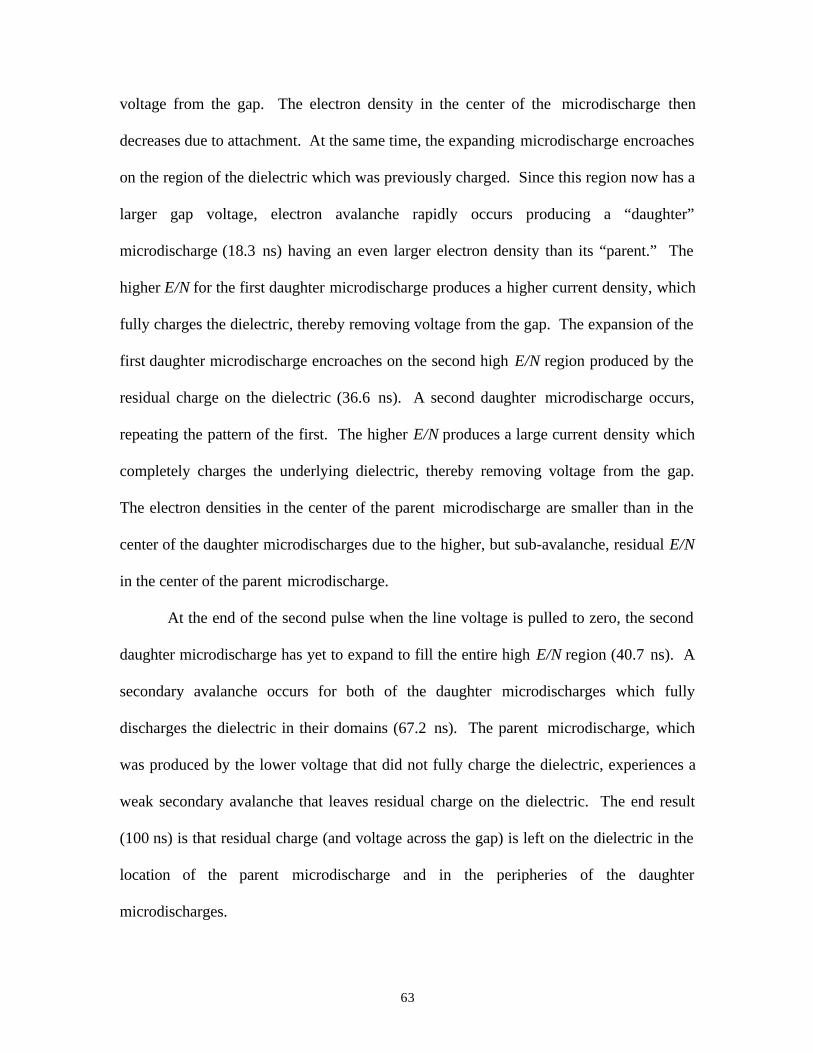
63
voltage from the gap. The electron density in the center of the microdischarge then
decreases due to attachment. At the same time, the expanding microdischarge encroaches
on the region of the dielectric which was previously charged. Since this region now has a
larger gap voltage, electron avalanche rapidly occurs producing a “daughter”
microdischarge (18.3 ns) having an even larger electron density than its “parent.” The
higher E/N for the first daughter microdischarge produces a higher current density, which
fully charges the dielectric, thereby removing voltage from the gap. The expansion of the
first daughter microdischarge encroaches on the second high E/N region produced by the
residual charge on the dielectric (36.6 ns). A second daughter microdischarge occurs,
repeating the pattern of the first. The higher E/N produces a large current density which
completely charges the underlying dielectric, thereby removing voltage from the gap.
The electron densities in the center of the parent microdischarge are smaller than in the
center of the daughter microdischarges due to the higher, but sub-avalanche, residual E/N
in the center of the parent microdischarge.
At the end of the second pulse when the line voltage is pulled to zero, the second
daughter microdischarge has yet to expand to fill the entire high E/N region (40.7 ns). A
secondary avalanche occurs for both of the daughter microdischarges which fully
discharges the dielectric in their domains (67.2 ns). The parent microdischarge, which
was produced by the lower voltage that did not fully charge the dielectric, experiences a
weak secondary avalanche that leaves residual charge on the dielectric. The end result
(100 ns) is that residual charge (and voltage across the gap) is left on the dielectric in the
location of the parent microdischarge and in the peripheries of the daughter
microdischarges.
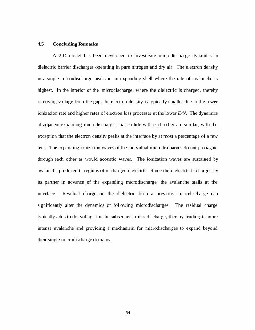
64
4.5 Concluding Remarks
A 2-D model has been developed to investigate microdischarge dynamics in
dielectric barrier discharges operating in pure nitrogen and dry air. The electron density
in a single microdischarge peaks in an expanding shell where the rate of avalanche is
highest. In the interior of the microdischarge, where the dielectric is charged, thereby
removing voltage from the gap, the electron density is typically smaller due to the lower
ionization rate and higher rates of electron loss processes at the lower E/N. The dynamics
of adjacent expanding microdischarges that collide with each other are similar, with the
exception that the electron density peaks at the interface by at most a percentage of a few
tens. The expanding ionization waves of the individual microdischarges do not propagate
through each other as would acoustic waves. The ionization waves are sustained by
avalanche produced in regions of uncharged dielectric. Since the dielectric is charged by
its partner in advance of the expanding microdischarge, the avalanche stalls at the
interface. Residual charge on the dielectric from a previous microdischarge can
significantly alter the dynamics of following microdischarges. The residual charge
typically adds to the voltage for the subsequent microdischarge, thereby leading to more
intense avalanche and providing a mechanism for microdischarges to expand beyond
their single microdischarge domains.
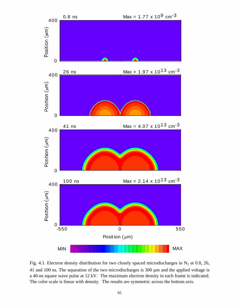
400
0
0-550 550
Position (µm)
0.8 ns Max = 1.77 x 109 cm-3
400
0
400
0
400
0
26 ns Max = 1.97 x 1013 cm-3
41 ns Max = 4.07 x 1013 cm-3
100 ns Max = 2.14 x 1013 cm-3
MIN MAX
Fig. 4.1. Electron density distribution for two closely spaced microdischarges in N2 at 0.8, 26,
41 and 100 ns. The separation of the two microdischarges is 300 µm and the applied voltage isa 40-ns square wave pulse at 12 kV. The maximum electron density in each frame is indicated.The color scale is linear with density. The results are symmetric across the bottom axis.
65
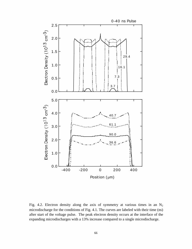
0.0
0.5
1.0
1.5
2.0
2.50-40 ns Pulse
3.7
7.3
16.1
29.4
0-200 400200-400
Position (µm)
36.6
40.7
61.1
90.0
0.0
1.0
2.0
3.0
4.0
5.0
Fig. 4.2. Electron density along the axis of symmetry at various times in an N2
microdischarge for the conditions of Fig. 4.1. The curves are labeled with their time (ns)after start of the voltage pulse. The peak electron density occurs at the interface of theexpanding microdischarges with a 13% increase compared to a single microdischarge.
66
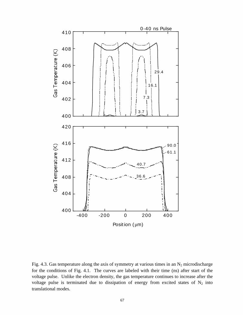
400
402
404
406
408
4100-40 ns Pulse
3.7
7.3
16.1
29.4
0-200 400200-400
Position (µm)
36.6
40.7
61.1
90.0
400
404
408
412
416
420
Fig. 4.3. Gas temperature along the axis of symmetry at various times in an N2 microdischargefor the conditions of Fig. 4.1. The curves are labeled with their time (ns) after start of thevoltage pulse. Unlike the electron density, the gas temperature continues to increase after thevoltage pulse is terminated due to dissipation of energy from excited states of N2 intotranslational modes.
67
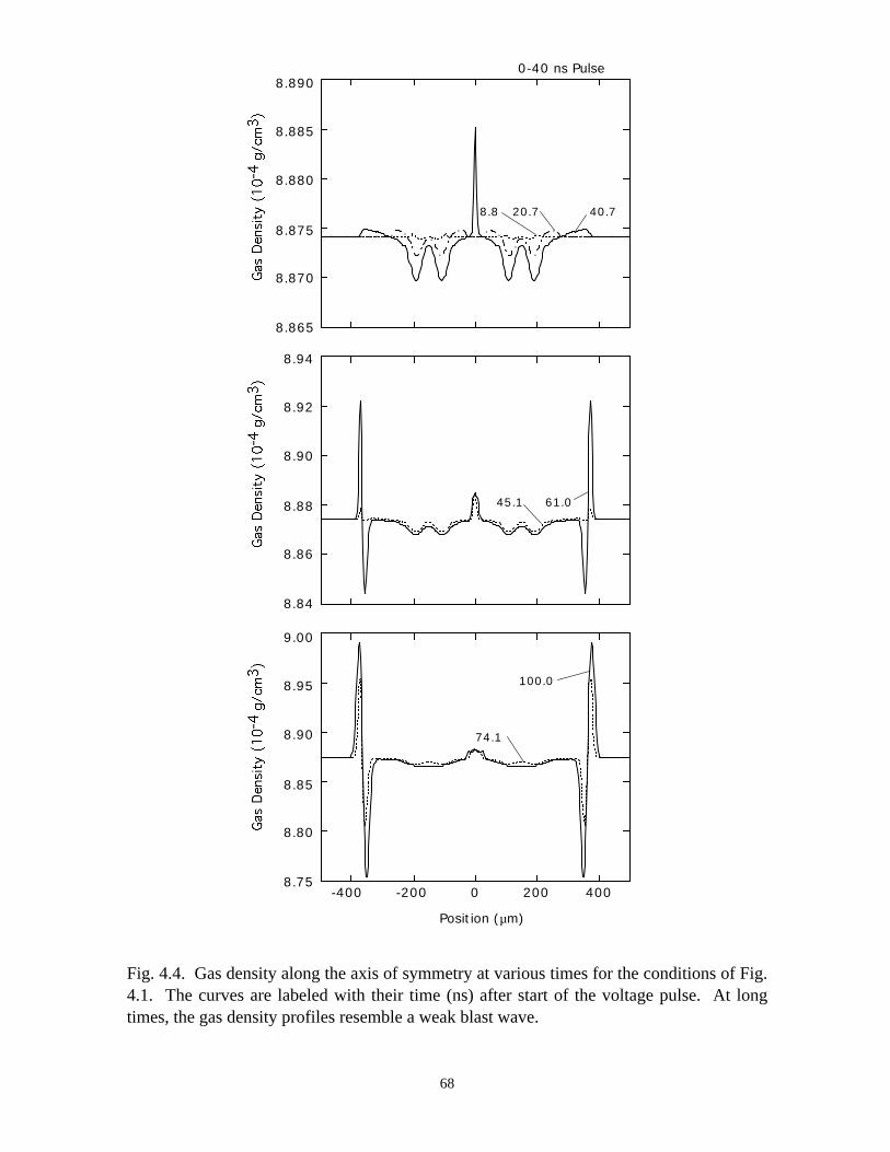
8.865
8.870
8.875
8.880
8.885
8.8900-40 ns Pulse
8.8 40.720.7
0-200 400200-400
Position (µm)
45.1 61.0
8.84
8.86
8.88
8.90
8.92
8.94
8.75
8.80
8.85
8.90
8.95
9.00
74.1
100.0
Fig. 4.4. Gas density along the axis of symmetry at various times for the conditions of Fig.4.1. The curves are labeled with their time (ns) after start of the voltage pulse. At longtimes, the gas density profiles resemble a weak blast wave.
68
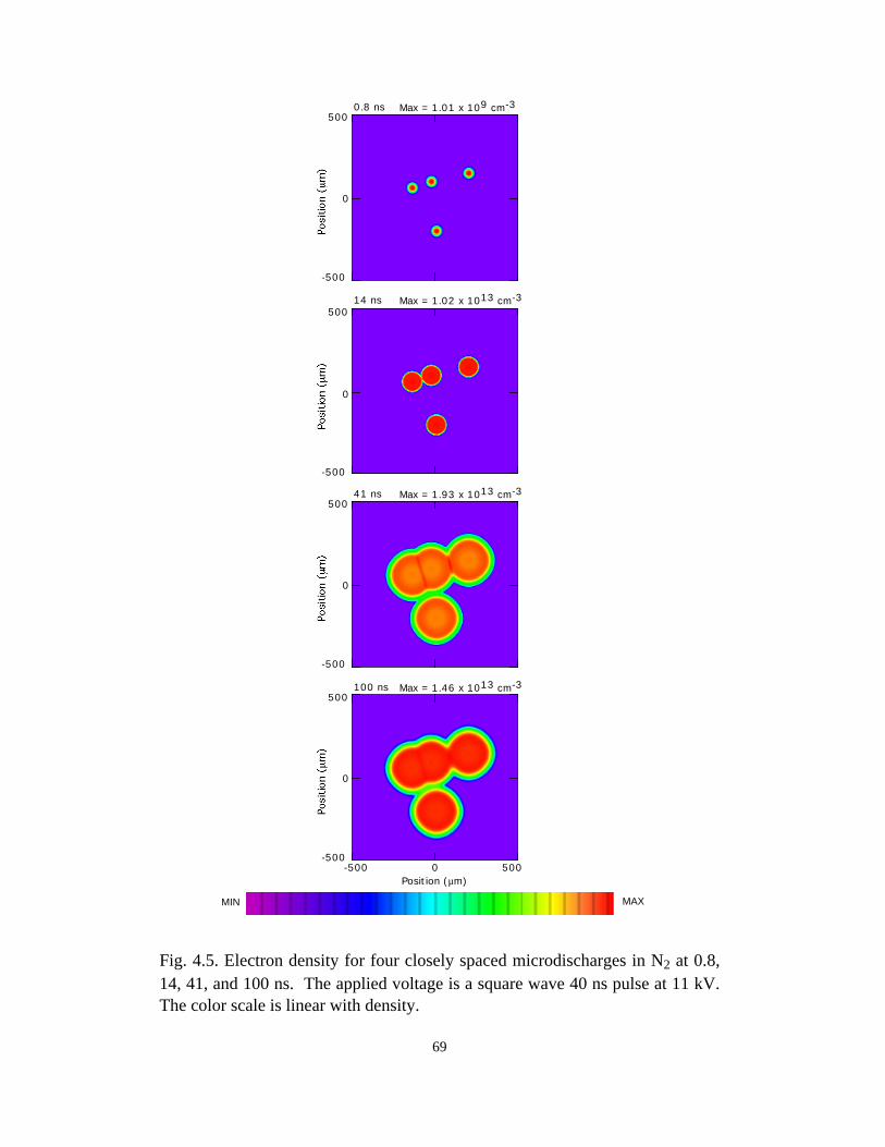
0.8 ns Max = 1.01 x 109 cm-3500
0
-500
14 ns Max = 1.02 x 1013 cm-3500
0
-500
41 ns Max = 1.93 x 1013 cm-3500
0
-500
100 ns Max = 1.46 x 1013 cm-3500
0
-500
Position (µm)5000-500
MIN
Fig. 4.5. Electron density for four closely spaced microdischarges in N2 at 0.8,14, 41, and 100 ns. The applied voltage is a square wave 40 ns pulse at 11 kV.The color scale is linear with density.
69
MAX
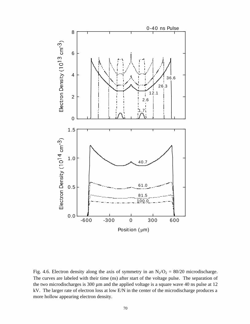
0
2
4
6
80-40 ns Pulse
1.7
2.6
12.1
26.3
0-300 600300-600
Position (µm)
81.5
40.7
61.0
100.0
0.0
0.5
1.0
1.5
36.6
Fig. 4.6. Electron density along the axis of symmetry in an N2/O2 = 80/20 microdischarge.The curves are labeled with their time (ns) after start of the voltage pulse. The separation ofthe two microdischarges is 300 µm and the applied voltage is a square wave 40 ns pulse at 12kV. The larger rate of electron loss at low E/N in the center of the microdischarge produces amore hollow appearing electron density.
70
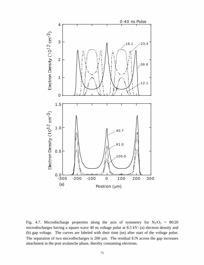
0
1
2
3
40-40 ns Pulse
1.7
16.1
12.1
23.4
61.0
40.7
100.0
0.0
0.5
1.0
1.5
36.6
Position (µm)
0-100 200100-200-300 300(a)
Fig. 4.7. Microdischarge properties along the axis of symmetry for N2/O2 = 80/20microdischarges having a square wave 40 ns voltage pulse at 8.5 kV: (a) electron density and(b) gap voltage. The curves are labeled with their time (ns) after start of the voltage pulse.
The separation of two microdischarges is 200 µm. The residual E/N across the gap increasesattachment in the post avalanche phase, thereby consuming electrons.
71
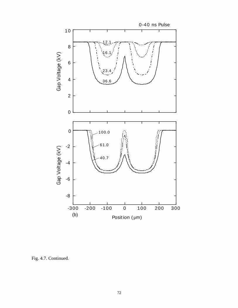
0-40 ns Pulse
23.4
12.1
16.1
40.7
61.0
100.0
36.6
0
2
4
6
8
10
Position (µm)
0-100 200100-200-300 300
0
-2
-4
-6
-8
(b)
Fig. 4.7. Continued.
72
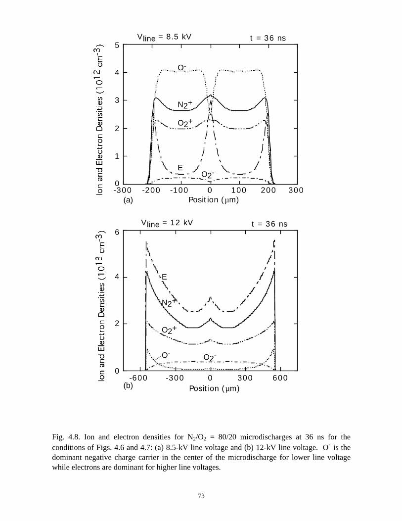
t = 36 ns
0-300 600300-600Position (µm)
0
1
2
3
4
5Vline = 8.5 kV
O-
N2+
O2+
EO2-
Position (µm)0-100 200100-200-300 300
0
2
4
6 t = 36 nsVline = 12 kV
O-
N2+
O2+
E
O2-
(a)
(b)
Fig. 4.8. Ion and electron densities for N2/O2 = 80/20 microdischarges at 36 ns for theconditions of Figs. 4.6 and 4.7: (a) 8.5-kV line voltage and (b) 12-kV line voltage. O is thedominant negative charge carrier in the center of the microdischarge for lower line voltagewhile electrons are dominant for higher line voltages.
73
-
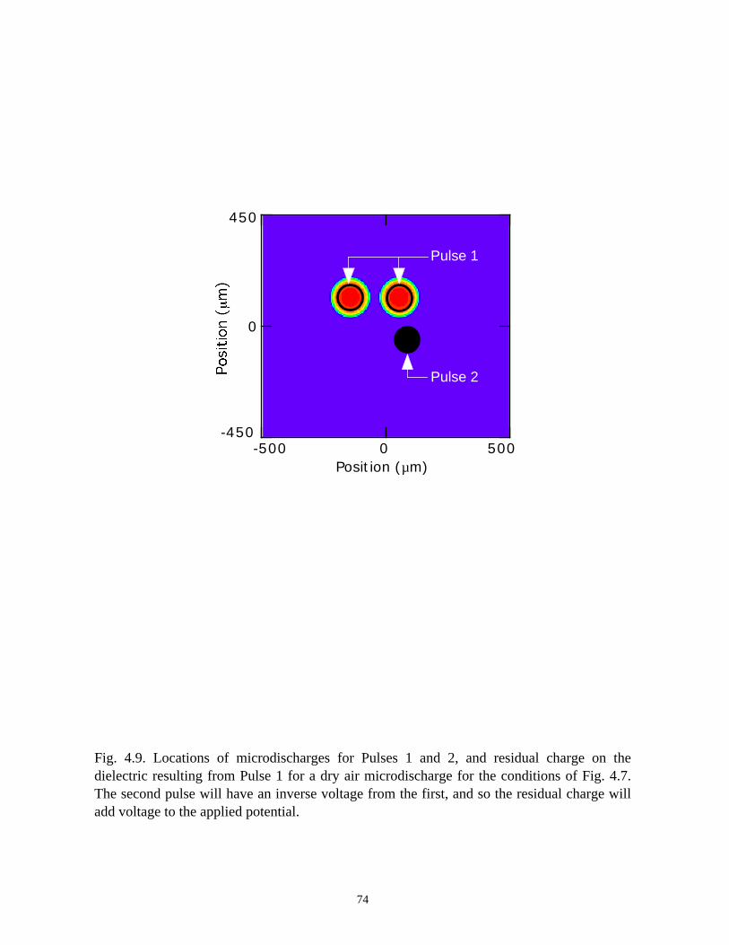
Pulse 1
Pulse 2
450
0
-450
Position (µm)5000-500
Fig. 4.9. Locations of microdischarges for Pulses 1 and 2, and residual charge on thedielectric resulting from Pulse 1 for a dry air microdischarge for the conditions of Fig. 4.7.The second pulse will have an inverse voltage from the first, and so the residual charge willadd voltage to the applied potential.
74
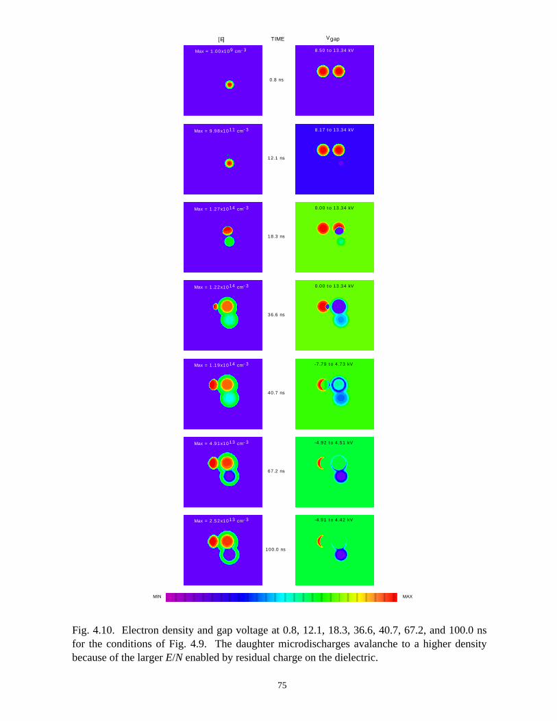
[E] Vgap
Max = 1.00x109 cm- 3
0.8 ns
8.50 to 13.34 kV
Max = 9.98x1011 cm- 3 8.17 to 13.34 kV
Max = 1.27x1014 cm- 3 0.00 to 13.34 kV
Max = 1.22x1014 cm- 3 0.00 to 13.34 kV
Max = 1.19x1014 cm- 3 -7.79 to 4.73 kV
Max = 4.91x1013 cm- 3 -4.92 to 4.51 kV
Max = 2.52x1013 cm- 3 -4.91 to 4.42 kV
12.1 ns
18.3 ns
36.6 ns
40.7 ns
67.2 ns
100.0 ns
TIME
MIN MAX
Fig. 4.10. Electron density and gap voltage at 0.8, 12.1, 18.3, 36.6, 40.7, 67.2, and 100.0 nsfor the conditions of Fig. 4.9. The daughter microdischarges avalanche to a higher densitybecause of the larger E/N enabled by residual charge on the dielectric.
75
76
5. REMEDIATION OF CARBONTETRACHLORIDE IN DIELECTRICBARRIER DISCHARGES
5.1 Introduction
Carbon tetrachloride (CCl4) is primarily used as an industrial solvent. CCl4
contamination in the environment is a concern due to its long lifetime and the large
volumes in use. Under ambient conditions, CCl4 is not decomposed easily [1, 2]. In the
atmosphere, CCl4 is almost unreactive with the hydroxyl radical (OH) but can be
decomposed via direct photolysis in the stratosphere [3, 4]. The persistence of CCl4 in
the environment is of concern because it is a suspected human carcinogen and as a result
is an Environmental Protection Agency (EPA) priority pollutant [5, 6].
Several methods have been applied to the remediation of gas-phase CCl4 such as
incineration [7], reduction over metallic iron [8], and decomposition with low
temperature plasmas [9-13]. In particular, dielectric barrier discharges are attractive for
this purpose due to their ability to operate stably at atmospheric pressure and due to their
low-cost maintenance [9].
In Chapter 3 we have shown that the characteristics of microdischarge
development in Ar/O2/CCl4 was appreciably influenced by small amounts of CCl4. Due
to the large rate of dissociative attachment of CCl4 at low E/N, electron densities showed
an expanding shell with a core composed of largely negative ions and positive ions. In
this chapter, we examine the kinetics and mechanism of plasma remediation of CCl4 in
Ar/O2 and Ar/O2/H2O gas mixtures in DBDs and determine the optimum strategies for its
remediation.
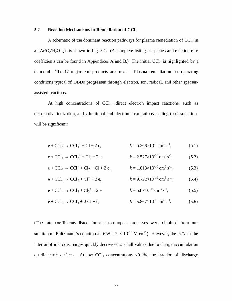
77
5.2 Reaction Mechanisms in Remediation of CCl4
A schematic of the dominant reaction pathways for plasma remediation of CCl4 in
an Ar/O2/H2O gas is shown in Fig. 5.1. (A complete listing of species and reaction rate
coefficients can be found in Appendices A and B.) The initial CCl4 is highlighted by a
diamond. The 12 major end products are boxed. Plasma remediation for operating
conditions typical of DBDs progresses through electron, ion, radical, and other species-
assisted reactions.
At high concentrations of CCl4, direct electron impact reactions, such as
dissociative ionization, and vibrational and electronic excitations leading to dissociation,
will be significant:
e + CCl4 → CCl3+ + Cl + 2 e, k = 5.268×10⁻⁹ cm3 s-1, (5.1)
e + CCl4 → CCl2+ + Cl2 + 2 e, k = 2.527×10⁻¹⁰ cm3 s-1, (5.2)
e + CCl4 → CCl+ + Cl2 + Cl + 2 e, k = 1.013×10⁻¹⁰ cm3 s-1, (5.3)
e + CCl4 → CCl3 + Cl+ + 2 e, k = 9.722×10⁻¹² cm3 s-1, (5.4)
e + CCl4 → CCl2 + Cl2+ + 2 e, k = 5.8×10⁻¹³ cm3 s-1, (5.5)
e + CCl4 → CCl2 + 2 Cl + e, k = 5.867×10⁻⁸ cm3 s-1. (5.6)
(The rate coefficients listed for electron-impact processes were obtained from our
solution of Boltzmann’s equation at E/N = 2 × 10-15 V cm2.) However, the E/N in the
interior of microdischarges quickly decreases to small values due to charge accumulation
on dielectric surfaces. At low CCl4 concentrations <0.1%, the fraction of discharge
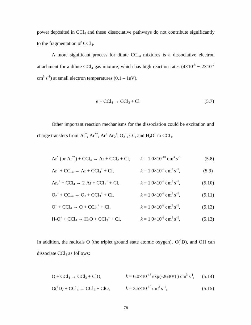
78
power deposited in CCl4 and these dissociative pathways do not contribute significantly
to the fragmentation of CCl4.
A more significant process for dilute CCl4 mixtures is a dissociative electron
attachment for a dilute CCl4 gas mixture, which has high reaction rates (4×10⁻⁸ − 2×10⁻⁷
cm3 s-1) at small electron temperatures (0.1 – 1eV).
e + CCl4 → CCl3 + Cl- (5.7)
Other important reaction mechanisms for the dissociation could be excitation and
charge transfers from Ar*, Ar**, Ar+ Ar2+, O2
+, O+, and H2O+ to CCl4.
Ar* (or Ar**) + CCl4 → Ar + CCl2 + Cl2 k = 1.0×10⁻¹⁰ cm3 s-1 (5.8)
Ar+ + CCl4 → Ar + CCl3+ + Cl, k = 1.0×10⁻⁹ cm3 s-1, (5.9)
Ar2+ + CCl4 → 2 Ar + CCl3
+ + Cl, k = 1.0×10⁻⁹ cm3 s-1, (5.10)
O2+ + CCl4 → O2 + CCl3
+ + Cl, k = 1.0×10⁻⁹ cm3 s-1, (5.11)
O+ + CCl4 → O + CCl3+ + Cl, k = 1.0×10⁻⁹ cm3 s-1, (5.12)
H2O+ + CCl4 → H2O + CCl3
+ + Cl, k = 1.0×10⁻⁹ cm3 s-1. (5.13)
In addition, the radicals O (the triplet ground state atomic oxygen), O(1D), and OH can
dissociate CCl4 as follows:
O + CCl4 → CCl3 + ClO, k = 6.0×10⁻¹³ exp(-2630/T) cm3 s-1, (5.14)
O(1D) + CCl4 → CCl3 + ClO, k = 3.5×10⁻¹⁰ cm3 s-1, (5.15)
79
OH + CCl4 → CCl3 + HOCl, k = 1.0×10⁻¹² exp(-2320/T) cm3 s-1. (5.16)
However, at ambient temperatures the Reactions (5.14) and (5.16) have small rate
coefficients, and so the only Reaction (5.14) alone contributes significantly to the
dissociation of CCl4.
CCl3, one of the main fragments of CCl4 quickly reacts with O2 to form CCl3O2:
CCl3 + O2 + M → CCl3O2 + M k = 1.19×10⁻³² exp(1278/T) cm6 s-1. (5.17)
The CCl3O2 undergoes a chain reaction with Cl radical and produces phosgene (COCl2)
as one of the main end products [14, 15]:
CCl3O2 + Cl → CCl3O + ClO k = 1×10-12 cm3 s-1, (5.18)
CCl3O2 + CCl3O2 → 2 CCl3O + O2 k = 8.32×10⁻¹¹ cm3 s-1, (5.19)
CCl3O → COCl2 + Cl k = 4.0×10¹³ exp(-4600/T) s-1. (5.20)
Other possible pathways, which scavenge CCl3, are reactions with O and OH,
CCl3 + O → COCl2 + Cl k = 4.15×10⁻¹¹ cm3 s-1, (5.21)
CCl3 + OH → COCl2 + HCl k = 4.15×10⁻¹¹ cm3 s-1. (5.22)
Another important fragment of CCl4, CCl2, reacts with O atoms and OH radicals
to generate COCl and also slowly reacts with O2 to form COCl2.
80
CCl2 + O → COCl + Cl k = 1×10-11 cm3 s-1, (5.23)
CCl2 + OH → COCl + HCl k = 1×10-11 cm3 s-1, (5.24)
CCl2 + O2 → COCl2 + Cl k = 1×10-14 cm3 s-1. (5.25)
The COCl further reacts with O, O2, Cl, and OH to generate CO and CO2, the details of
which are summarized in Fig. 5.1. At ambient temperatures, CO and COCl2 are fairly
stable molecules, though COCl2 slowly reacts with O and OH.
The other end product is Cl2, which is formed by the reaction
Cl + Cl + M → Cl2 + M k = 3.47×10⁻³³ exp(810/T) cm6 s-1. (5.26)
Cl is produced mainly by the ion-ion neutralization reaction of Cl-.
5.3 Spatial Dependencies in Remediation of CCl4
In this section, we consider the dynamics of the system, focusing on CCl 4
remediation and the temporal and spatial dependencies of important species. In the
analyses that follow, a single streamer is examined using the 1-D radially dependent
model as described in Section 2.2. Furthermore, we limit the discharge to the first pulse
only. The standard conditions used in this chapter are the same as those used in Chapter
3 (the applied voltage is a square pulse with 40 ns duration, the initial gas pressure is 1
atm, and the initial seed electron density has a distribution 20 µm in radius and 109 cm-3
81
peak value), with the exception that the temperature is 300 K. The baseline case is a gas
mixture of Ar/O2/CCl4 = 79.9/20/0.1 with a pulse magnitude of 12 kV.
The production of charged species is the main process during the pulse. Figure
5.2 shows the concentration profiles of the electron, positive ions, and negative ions
during and following the voltage pulse as a function of radius. During the 40-ns voltage
pulse, the electron density sharply peaks at the edge of the microdischarge because
electrons are rapidly consumed, primarily by the dissociative attachment to CCl4 in the
core. The Cl-, on the other hand, shows a flat distribution in the core. Electrons also
attach to oxygen to generate O- and O2-, whose concentrations are 12 and 25 times less
than the Cl- concentration during the pulse. Due to the low CCl4 concentration (0.01
mole fraction), the direct electron impact ionization of CCl4 is negligible. The major
ionization reactions involving electrons are those of Ar and O2,
e + Ar → Ar+ + 2 e, k = 1.18×10⁻¹⁰ cm3 s-1, (5.27)
e + O2 → O2+ + 2 e, k = 1.77×10⁻¹⁰ cm3 s-1, (5.28)
e + O2 → O+ + O + 2 e, k = 1.45×10⁻¹² cm3 s-1, (5.29)
where the rate coefficients are for E/N = 2×10-15 V cm2. It is apparent that Ar+ and O2+
are the primary ions generated by electron impact. Ar+ is rapidly depleted due to its
charge transfer reactions,
Ar+ + CCl4 → Ar + CCl3+ + Cl, k = 1.0×10⁻⁹ cm3 s-1, (5.30)
Ar+ + O2 → Ar + O2+, k = 4.0×10⁻¹¹ cm3 s-1, (5.31)
Ar+ + Ar + M → Ar2+ + M, k = 2.0×10⁻³¹ cm6 s-1, (5.32)
82
Most of Ar+ are consumed by the charge transfer reaction with O2 [Reaction (5.31)]. The
dime ion, Ar2+, also rapidly transfers its charge. Both of Ar+ and Ar2
+ densities have a
sharp edge in their profiles [Fig. 5.2(e) and (f)]. O2+ depletion by charge transfer is only
by the reaction with CCl4. The O2+ density profile displays a much less sharp edge than
Ar+ and Ar2+. The CCl3
+ density shows a steady decrease, with increasing radius during
the pulse and a flatter profile within the core after the pulse.
The excited state species Ar*, Ar**, and O(1D), which can decompose CCl4, are
shown in Fig. 5.3. All of their densities have a sharp edge. Because of the larger
concentration of O2 compared to CCl4, these species are lost preferentially to quenching
by O2 and so do not make an important contribution to CCl4 decomposition. Compared
to O(1D) in Fig. 5.3(c), the triplet state of atomic oxygen O, shown in Fig. 5.3(d), has
higher concentration (by a factor of 3.6) with a flat spatial distribution. O reacts with O2,
CCl3, and CCl2 to generate O3, COCl2, and COCl, respectively.
The spatial dependence of the CCl3, CCl2, and Cl densities, the primary neutral
fragments of CCl4 are shown in Fig. 5.4. Since CCl 3 is scavenged rapidly by O2 [as in
Reaction (5.17)], the CCl3 density shows a hollow distribution. During the pulse, the
peak value of CCl3 is more than that of CCl2 by a factor of 5. The CCl3 radicals are
almost removed completely at around 5 µs. Unlike the CCl3, the CCl2 is uniformly
distributed within the core. The CCl2 concentration builds up during the leading and
trailing edge of the pulse due to the reactions of excited species such as Ar* and Ar** with
CCl4 to form CCl2 [Reaction (5.8)] and the electron-impact dissociation of CCl 4
[Reaction (5.6)]. The CCl2 density gradually decreases after the pulse because there is a
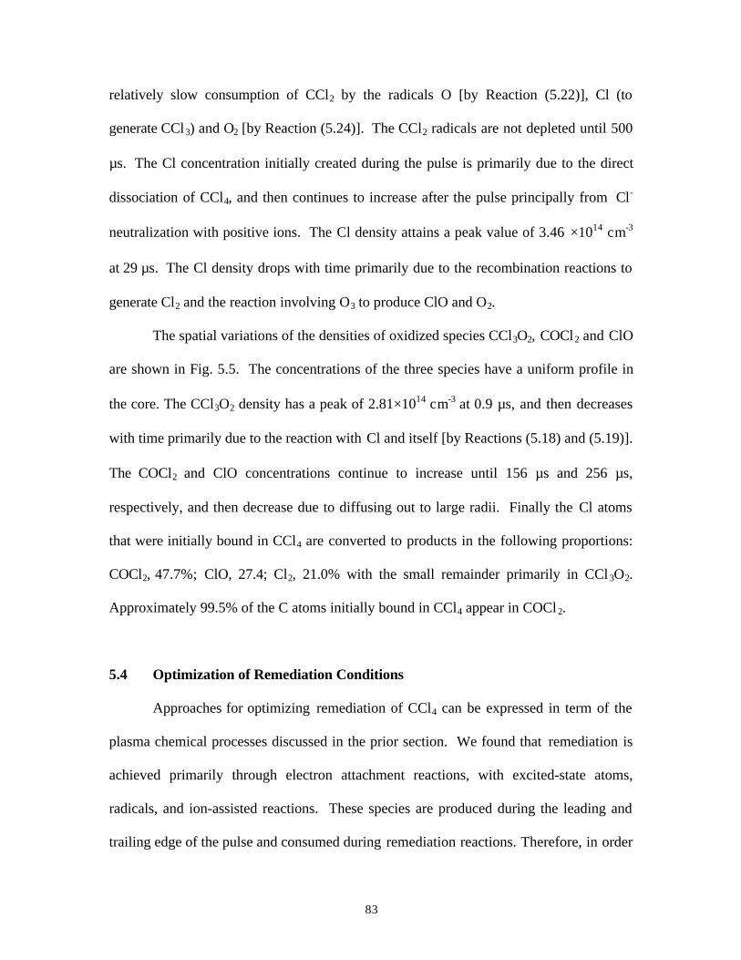
83
relatively slow consumption of CCl2 by the radicals O [by Reaction (5.22)], Cl (to
generate CCl3) and O2 [by Reaction (5.24)]. The CCl2 radicals are not depleted until 500
µs. The Cl concentration initially created during the pulse is primarily due to the direct
dissociation of CCl4, and then continues to increase after the pulse principally from Cl-
neutralization with positive ions. The Cl density attains a peak value of 3.46 ×1014 cm-3
at 29 µs. The Cl density drops with time primarily due to the recombination reactions to
generate Cl2 and the reaction involving O3 to produce ClO and O2.
The spatial variations of the densities of oxidized species CCl3O2, COCl2 and ClO
are shown in Fig. 5.5. The concentrations of the three species have a uniform profile in
the core. The CCl3O2 density has a peak of 2.81×1014 cm-3 at 0.9 µs, and then decreases
with time primarily due to the reaction with Cl and itself [by Reactions (5.18) and (5.19)].
The COCl2 and ClO concentrations continue to increase until 156 µs and 256 µs,
respectively, and then decrease due to diffusing out to large radii. Finally the Cl atoms
that were initially bound in CCl4 are converted to products in the following proportions:
COCl2, 47.7%; ClO, 27.4; Cl2, 21.0% with the small remainder primarily in CCl3O2.
Approximately 99.5% of the C atoms initially bound in CCl4 appear in COCl2.
5.4 Optimization of Remediation Conditions
Approaches for optimizing remediation of CCl4 can be expressed in term of the
plasma chemical processes discussed in the prior section. We found that remediation is
achieved primarily through electron attachment reactions, with excited-state atoms,
radicals, and ion-assisted reactions. These species are produced during the leading and
trailing edge of the pulse and consumed during remediation reactions. Therefore, in order

84
to obtain an optimal remediation strategy, it is important to consider the effects of all the
parameters that affect the formation and depletion of agents that remediate CCl4.
To explore these dependencies we parameterized the model over the capacitance
of dielectric (εd/L, where εd = permittivity, L = thickness of the dielectric), applied
voltage, and O2 mole fraction. Further, we will examine effects of water vapor on CCl 4
remediation in the next section. To evaluate the efficiency of remediation, the results
have been summarized in the term of eV/molecule: the amount of energy (eV) required
removing 1 molecule of CCl4, typically called the W value. Thus, the lower the W value,
the more efficient is the process.
Energy deposition and the W value for CCl4 degradation are shown in Fig. 5.6 as
a function of dielectric capacitance, where the conditions for each case are the same as
that of the standard case in Section 5.3, with the exception of the dielectric capacitance
being varied. As might be anticipated, the energy deposition linearly increases with
increasing the dielectric capacitance. However, the W value increases with increasing
εd/L due to a less efficient utilization of the reactant intermediates. Electrons, Ar+, O2+,
Ar*, Ar**, and O(1D), which do not quickly react with CCl4, will be otherwise consumed.
The W value decreases at high applied voltages, as shown in Fig. 5.7, where the
conditions for each case are the same as the standard case of Section 5.3 with the
exception that the applied voltage is varied. This scaling results from the fact that the
fractional power deposition producing ionization, excitation and dissociation increases
with increasing E/N, especially for ionization due to the generation of more electrons,
which are beneficial to CCl4 dissociation.
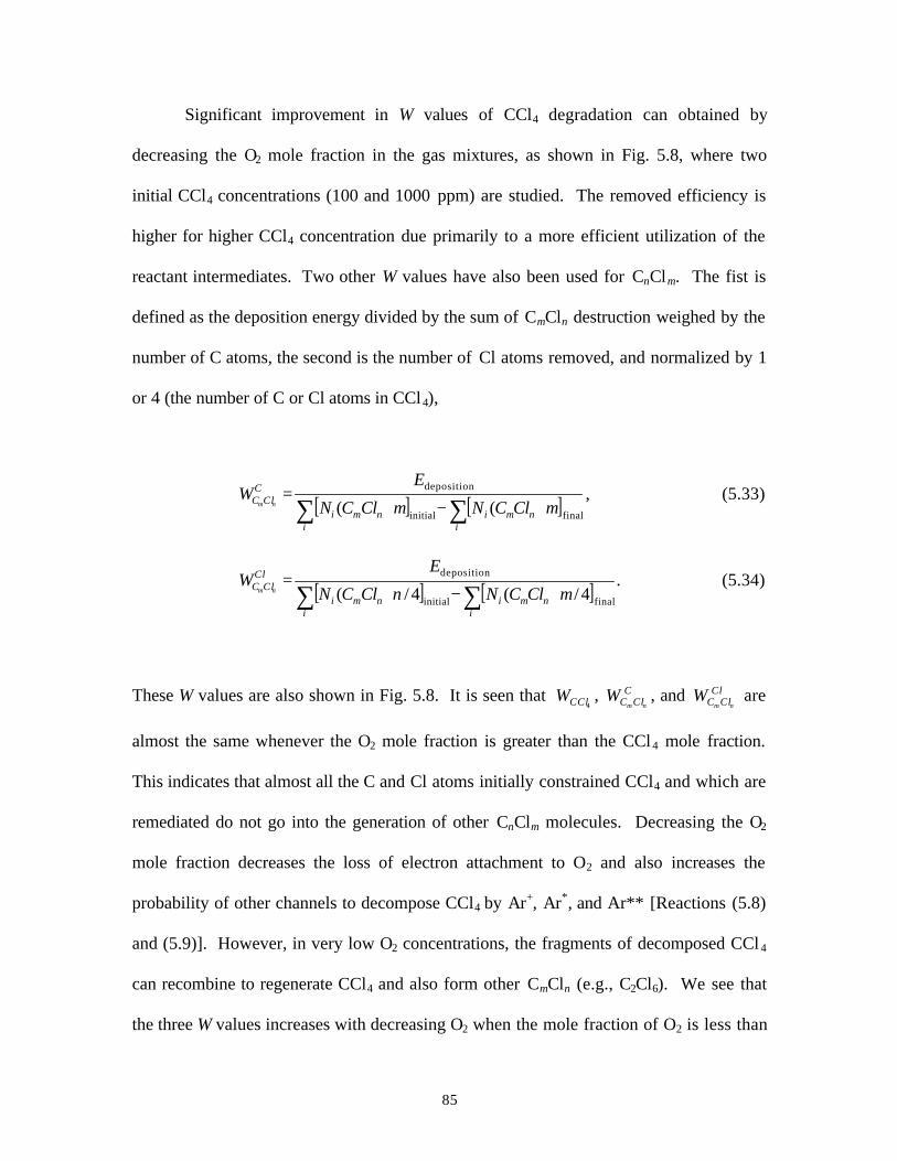
85
Significant improvement in W values of CCl4 degradation can obtained by
decreasing the O2 mole fraction in the gas mixtures, as shown in Fig. 5.8, where two
initial CCl4 concentrations (100 and 1000 ppm) are studied. The removed efficiency is
higher for higher CCl4 concentration due primarily to a more efficient utilization of the
reactant intermediates. Two other W values have also been used for CnClm. The fist is
defined as the deposition energy divided by the sum of CmCln destruction weighed by the
number of C atoms, the second is the number of Cl atoms removed, and normalized by 1
or 4 (the number of C or Cl atoms in CCl4),
[ ] [ ]∑ ∑ ⋅−⋅=
i inminmi
CClC mClCNmClCN
EW
nm
finalinitial
deposition
((, (5.33)
[ ] [ ]∑ ∑ ⋅−⋅=
i inminmi
ClClC mClCNnClCN
EW
nm
finalinitial
deposition
4/(4/(. (5.34)
These W values are also shown in Fig. 5.8. It is seen that 4CClW , C
ClC nmW , and Cl
ClC nmW are
almost the same whenever the O2 mole fraction is greater than the CCl4 mole fraction.
This indicates that almost all the C and Cl atoms initially constrained CCl4 and which are
remediated do not go into the generation of other CnClm molecules. Decreasing the O2
mole fraction decreases the loss of electron attachment to O2 and also increases the
probability of other channels to decompose CCl4 by Ar+, Ar*, and Ar** [Reactions (5.8)
and (5.9)]. However, in very low O2 concentrations, the fragments of decomposed CCl4
can recombine to regenerate CCl4 and also form other CmCln (e.g., C2Cl6). We see that
the three W values increases with decreasing O2 when the mole fraction of O2 is less than
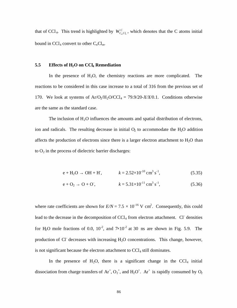
86
that of CCl4. This trend is highlighted by CClC nm
W , which denotes that the C atoms initial
bound in CCl4 convert to other CnClm.
5.5 Effects of H2O on CCl4 Remediation
In the presence of H2O, the chemistry reactions are more complicated. The
reactions to be considered in this case increase to a total of 316 from the previous set of
170. We look at systems of Ar/O2/H2O/CCl4 = 79.9/20-X/X/0.1. Conditions otherwise
are the same as the standard case.
The inclusion of H2O influences the amounts and spatial distribution of electrons,
ion and radicals. The resulting decrease in initial O2 to accommodate the H2O addition
affects the production of electrons since there is a larger electron attachment to H2O than
to O2 in the process of dielectric barrier discharges:
e + H2O → OH + H-, k = 2.52×10⁻¹⁰ cm3 s-1, (5.35)
e + O2 → O + O-, k = 5.31×10⁻¹¹ cm3 s-1, (5.36)
where rate coefficients are shown for E/N = 7.5 × 10⁻¹⁶ V cm2. Consequently, this could
lead to the decrease in the decomposition of CCl4 from electron attachment. Cl- densities
for H2O mole fractions of 0.0, 10-2, and 7×10⁻² at 30 ns are shown in Fig. 5.9. The
production of Cl- decreases with increasing H2O concentrations. This change, however,
is not significant because the electron attachment to CCl4 still dominates.
In the presence of H2O, there is a significant change in the CCl4 initial
dissociation from charge transfers of Ar+, O2+, and H2O
+. Ar+ is rapidly consumed by O2
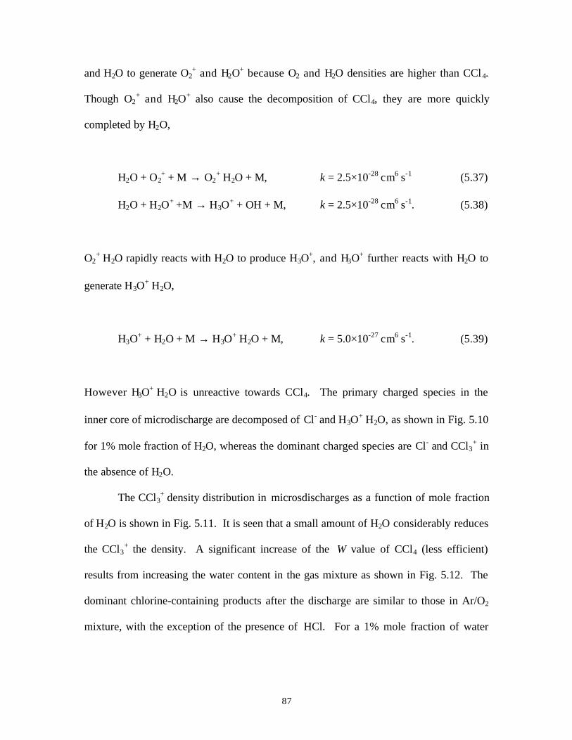
87
and H2O to generate O2+ and H2O
+ because O2 and H2O densities are higher than CCl4.
Though O2+ and H2O
+ also cause the decomposition of CCl4, they are more quickly
completed by H2O,
H2O + O2+ + M → O2
+⋅H2O + M, k = 2.5×10⁻²⁸ cm6 s-1 (5.37)
H2O + H2O+ +M → H3O
+ + OH + M, k = 2.5×10⁻²⁸ cm6 s-1. (5.38)
O2+⋅H2O rapidly reacts with H2O to produce H3O
+, and H3O+ further reacts with H2O to
generate H3O+⋅H2O,
H3O+ + H2O + M → H3O
+⋅H2O + M, k = 5.0×10⁻²⁷ cm6 s-1. (5.39)
However H3O+⋅H2O is unreactive towards CCl4. The primary charged species in the
inner core of microdischarge are decomposed of Cl- and H3O+⋅H2O, as shown in Fig. 5.10
for 1% mole fraction of H2O, whereas the dominant charged species are Cl- and CCl3+ in
the absence of H2O.
The CCl3+ density distribution in microsdischarges as a function of mole fraction
of H2O is shown in Fig. 5.11. It is seen that a small amount of H2O considerably reduces
the CCl3+ the density. A significant increase of the W value of CCl4 (less efficient)
results from increasing the water content in the gas mixture as shown in Fig. 5.12. The
dominant chlorine-containing products after the discharge are similar to those in Ar/O2
mixture, with the exception of the presence of HCl. For a 1% mole fraction of water
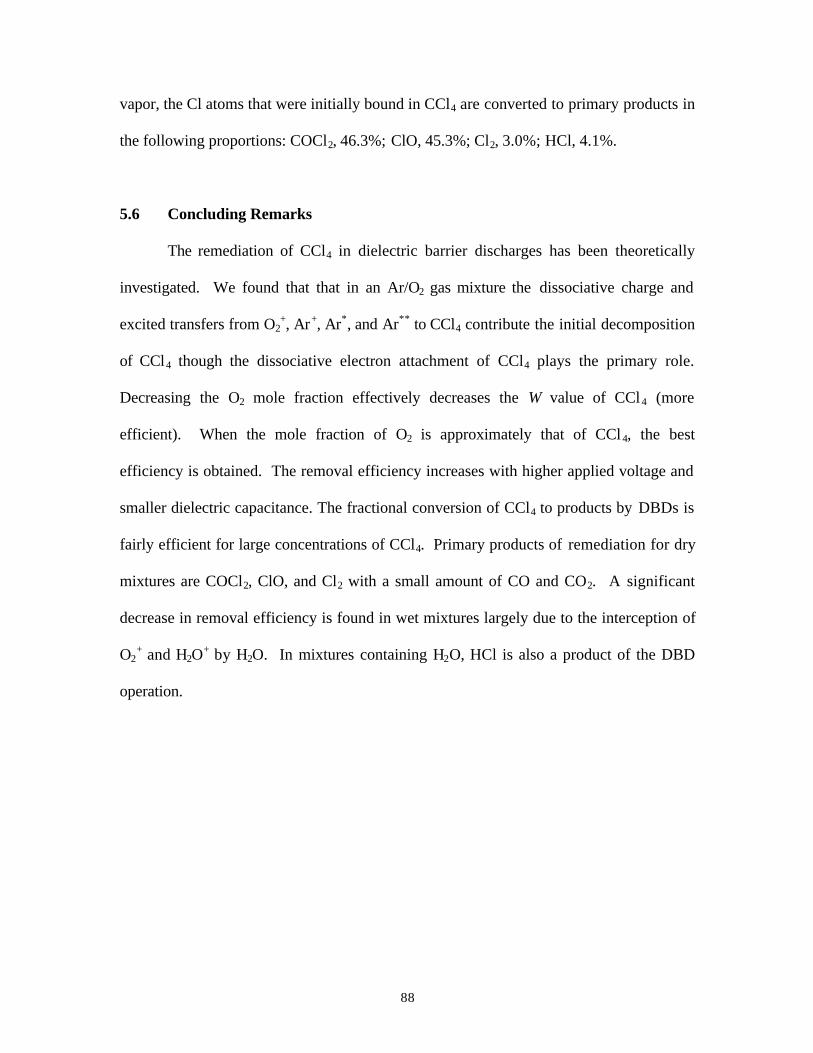
88
vapor, the Cl atoms that were initially bound in CCl4 are converted to primary products in
the following proportions: COCl2, 46.3%; ClO, 45.3%; Cl2, 3.0%; HCl, 4.1%.
5.6 Concluding Remarks
The remediation of CCl4 in dielectric barrier discharges has been theoretically
investigated. We found that that in an Ar/O2 gas mixture the dissociative charge and
excited transfers from O2+, Ar+, Ar*, and Ar** to CCl4 contribute the initial decomposition
of CCl4 though the dissociative electron attachment of CCl4 plays the primary role.
Decreasing the O2 mole fraction effectively decreases the W value of CCl4 (more
efficient). When the mole fraction of O2 is approximately that of CCl4, the best
efficiency is obtained. The removal efficiency increases with higher applied voltage and
smaller dielectric capacitance. The fractional conversion of CCl4 to products by DBDs is
fairly efficient for large concentrations of CCl4. Primary products of remediation for dry
mixtures are COCl2, ClO, and Cl2 with a small amount of CO and CO2. A significant
decrease in removal efficiency is found in wet mixtures largely due to the interception of
O2+ and H2O
+ by H2O. In mixtures containing H2O, HCl is also a product of the DBD
operation.
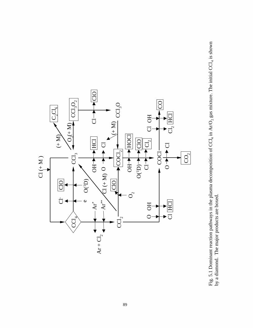
ClO
CC
l 4
eCl-
O(1 D
)
Ar*
Ar**
Ar
+ C
l 2
CO
Cl 2
CC
l 3
CC
l 2
OC
lO2
CC
l 3O2
Cl (
+ M
)
Cl (
+ M
)OH
HC
l
C2C
l 6
CO
Cl
O(1 D
)
OH
HO
Cl
O Cl
OH
HC
l
Cl
Cl 2
CO
Cl
Cl 2
OH
HC
l
CO
2
OC
l
(+ M
)
CC
l 3O
Cl
(+ M
)
(+ M
)
ClO
ClO
O2
ClO
Fig
. 5.1
Dom
inan
t rea
ctio
n pa
thw
ays
in th
e pl
asm
a de
com
posi
tion
of
CC
l 4 in
Ar/
O2 g
as m
ixtu
re. T
he in
itia
l CC
l 4 is
sho
wn
by a
dia
mon
d. T
he m
ajor
pro
duct
s ar
e bo
xed.
89
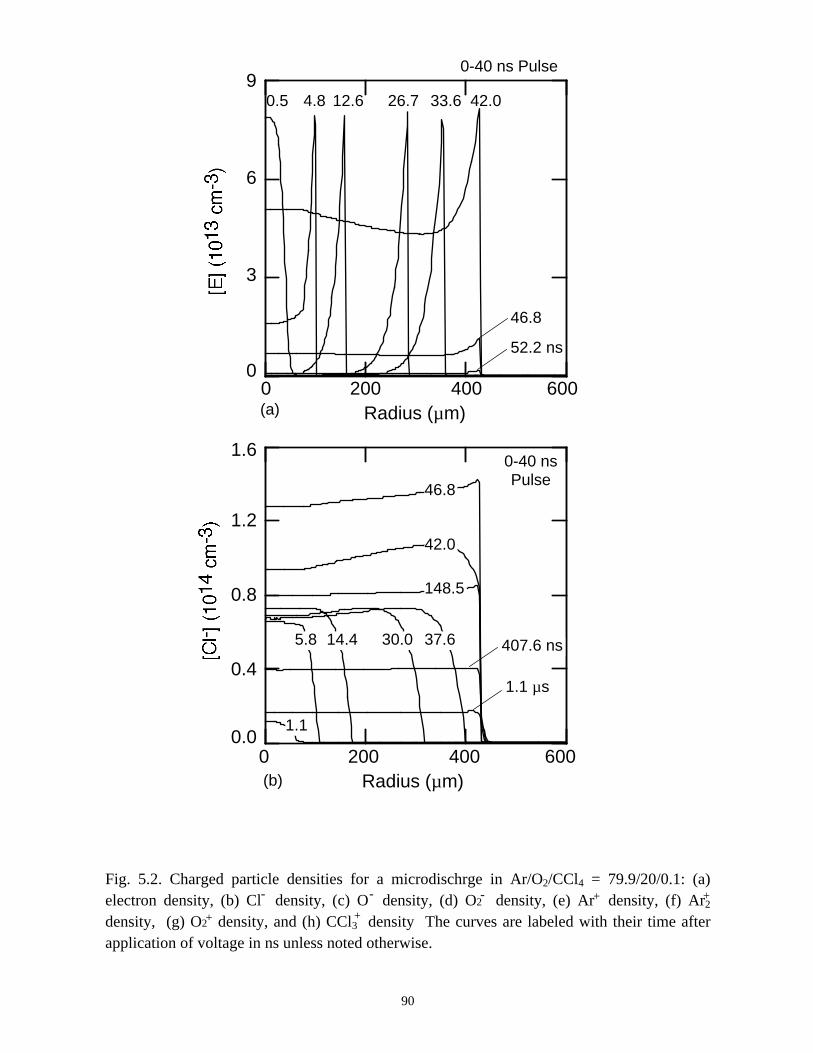
0.5 4.8 12.6 33.626.7 42.0
46.8
52.2 ns
3
0
6
9
0 200 400 600Radius (µm)
1.1
5.8 14.4 30.0 37.6
42.0
46.8
148.5
407.6 ns
1.1 µs
0 200 400 600Radius (µm)
0.0
0.4
0.8
1.2
1.6
0-40 ns Pulse
0-40 nsPulse
(a)
(b)
Fig. 5.2. Charged particle densities for a microdischrge in Ar/O2/CCl4 = 79.9/20/0.1: (a)electron density, (b) Cl density, (c) O density, (d) O2 density, (e) Ar density, (f) Ar2
density, (g) O2 density, and (h) CCl3 density The curves are labeled with their time afterapplication of voltage in ns unless noted otherwise.
90
- - - + +
+ +
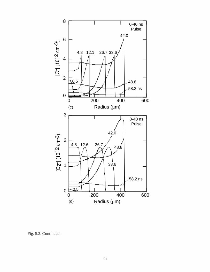
0.5
4.8 12.1 26.7 33.6
42.0
58.2 ns
0 200 400 600Radius (µm)
0
2
4
6
8
48.8
0.5
4.8 12.6
33.6
26.7
42.0
58.2 ns
48.8
0 200 400 600Radius (µm)
0
2
1
3
0-40 nsPulse
0-40 nsPulse
Fig. 5.2. Continued.
91
(c)
(d)
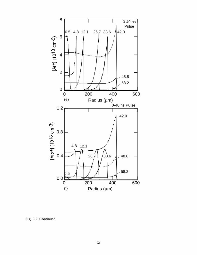
0.5 4.8 12.1 26.7 33.6 42.0
58.2
0 200 400 600Radius (µm)
0
2
4
6
8
48.8
Fig. 5.2. Continued.
92
0-40 nsPulse
(e)
0.5
4.8 12.1
26.7 33.6
42.0
58.2
0 200 400 600Radius (µm)
48.8
0.0
0.4
0.8
1.20-40 ns Pulse
(f)
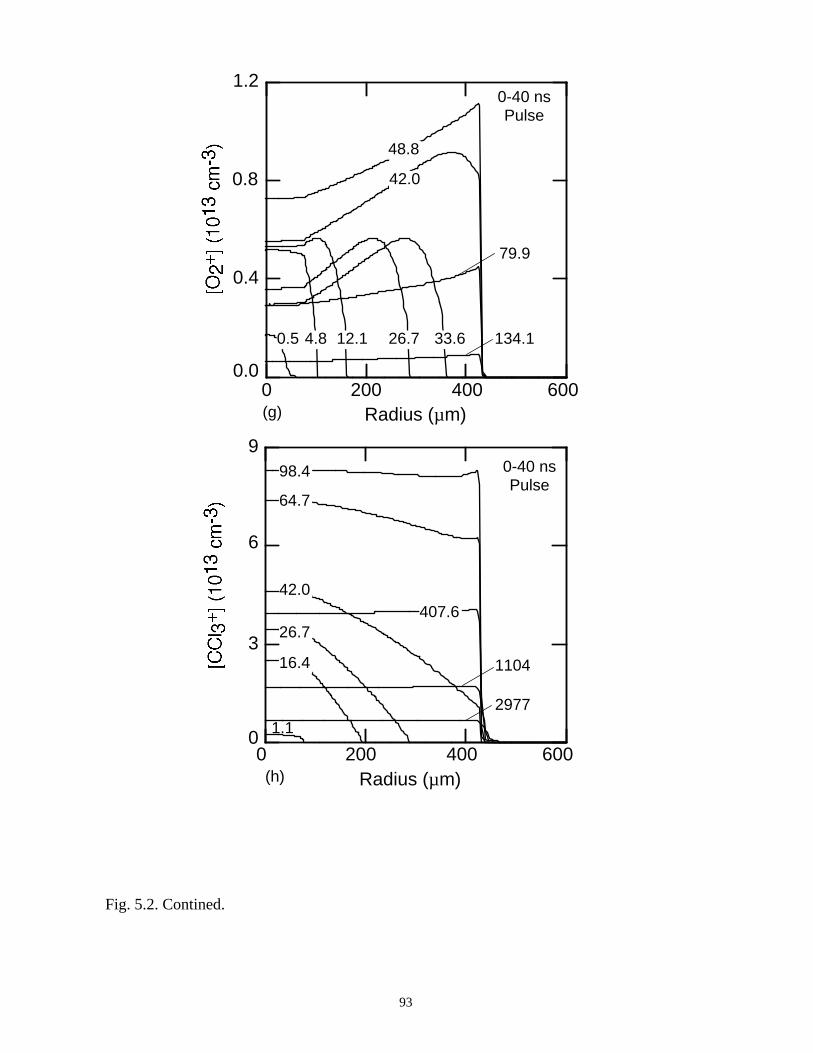
0 200 400 600Radius (µm)
0.0
0.4
0.8
1.2
0.5 4.8 12.1 26.7 33.6
42.0
48.8
79.9
134.1
1.1
16.4
26.7
64.7
42.0
98.4
1104
0 200 400 600Radius (µm)
0
3
9
6
407.6
2977
Fig. 5.2. Contined.
93
(g)
0-40 nsPulse
0-40 nsPulse
(h)

0 200 400 600Radius (µm)
0
2
4
0.5 4.8 12.6 33.626.7
42.0 ns
0-40 nsPulse
(a)
0.5 4.8 12.6 33.626.7
42.0 ns
0 200 400 600Radius (µm)
0.0
0.5
1.0
1.50-40 nsPulse
(b)
Fig. 5.3. (a) Ar* density, (b) Ar** density, (c) O(1D) density and (d) O density for theconditions of Fig. 5.2. The excited state species, Ar* and Ar*, lead to the decomposition ofCCl4 by the excitation transfer. CCl4 is almost not reacted with O but is decomposed byO(1D). The curves are labeled with their time after application of voltage (ns).
94
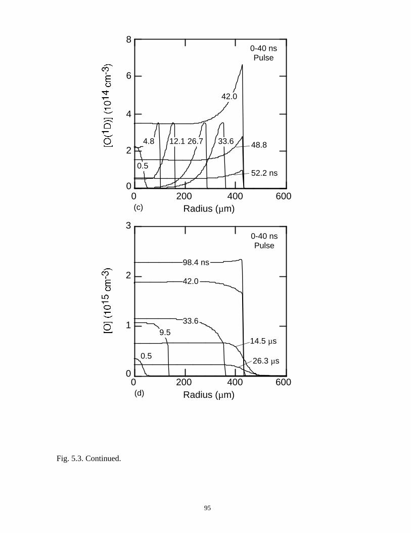
0
2
4
6
0.5
4.8 12.1 26.7 33.6
42.0
48.8
8
52.2 ns
0 200 400 600Radius (µm)
0-40 nsPulse
(c)
0.5
9.533.6
42.0
98.4 ns
14.5 µs
26.3 µs
0
1
2
3
0 200 400 600Radius (µm)
0-40 nsPulse
(d)
Fig. 5.3. Continued.
95
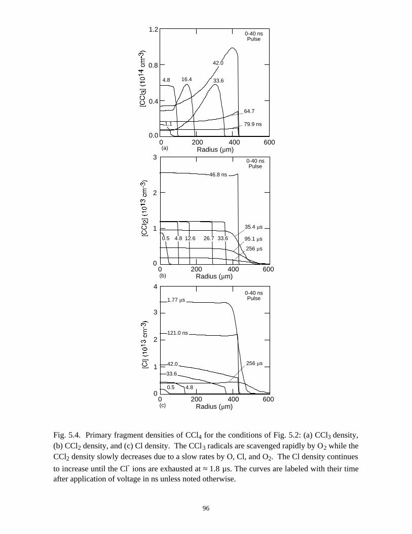
0 200 400 600Radius (µm)
0.0
0.4
0.8
1.2
1.1
4.8 16.4
64.7
33.6
42.0
79.9 ns
0-40 nsPulse
(a)
0.5 4.8 12.6 33.626.7
46.8 ns
35.4 µs
95.1 µs
256 µs
1
0
2
3
0 200 400 600Radius (µm)
0-40 nsPulse
(b)
0.5 4.8
33.6
42.0
121.0 ns
1.77 µs
256 µs1
0
2
3
4
0 200 400 600Radius (µm)
0-40 nsPulse
(c)
Fig. 5.4. Primary fragment densities of CCl4 for the conditions of Fig. 5.2: (a) CCl3 density,(b) CCl2 density, and (c) Cl density. The CCl3 radicals are scavenged rapidly by O2 while theCCl2 density slowly decreases due to a slow rates by O, Cl, and O2. The Cl density continues
to increase until the Cl ions are exhausted at ≈ 1.8 µs. The curves are labeled with their timeafter application of voltage in ns unless noted otherwise.
96
-
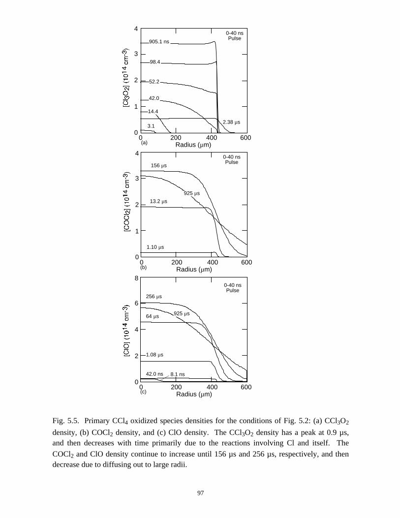
3.1
14.4
52.2
42.0
98.4
905.1 ns
2.38 µs
1
0
2
3
4
0 200 400 600Radius (µm)
0-40 nsPulse
(a)
1.10 µs
13.2 µs
156 µs
925 µs
1
0
2
3
4
0 200 400 600Radius (µm)
0-40 nsPulse
(b)
Radius (µm)
8.1 ns42.0 ns
1.08 µs
64 µs 925 µs
256 µs
2
0
4
6
8
0 200 400 600
0-40 nsPulse
(c)
Fig. 5.5. Primary CCl4 oxidized species densities for the conditions of Fig. 5.2: (a) CCl3O2
density, (b) COCl2 density, and (c) ClO density. The CCl3O2 density has a peak at 0.9 µs,and then decreases with time primarily due to the reactions involving Cl and itself. The
COCl2 and ClO density continue to increase until 156 µs and 256 µs, respectively, and thendecrease due to diffusing out to large radii.
97
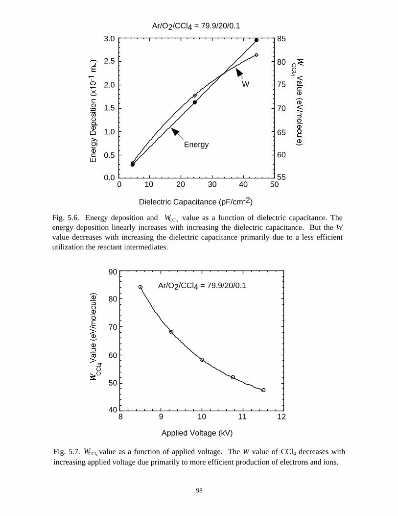
0 10 20 30 40 500.0
0.5
1.0
1.5
2.0
2.5
3.0
55
60
65
70
75
80
85
Dielectric Capacitance (pF/cm-2)
Ar/O2/CCl4 = 79.9/20/0.1
Energy
W
Fig. 5.6. Energy deposition and value as a function of dielectric capacitance. Theenergy deposition linearly increases with increasing the dielectric capacitance. But the Wvalue decreases with increasing the dielectric capacitance primarily due to a less efficientutilization the reactant intermediates.
8 9 10 11 1240
50
60
70
80
90
Applied Voltage (kV)
Ar/O2/CCl4 = 79.9/20/0.1
Fig. 5.7. value as a function of applied voltage. The W value of CCl4 decreases withincreasing applied voltage due primarily to more efficient production of electrons and ions.
98
WCCl4
WCCl4
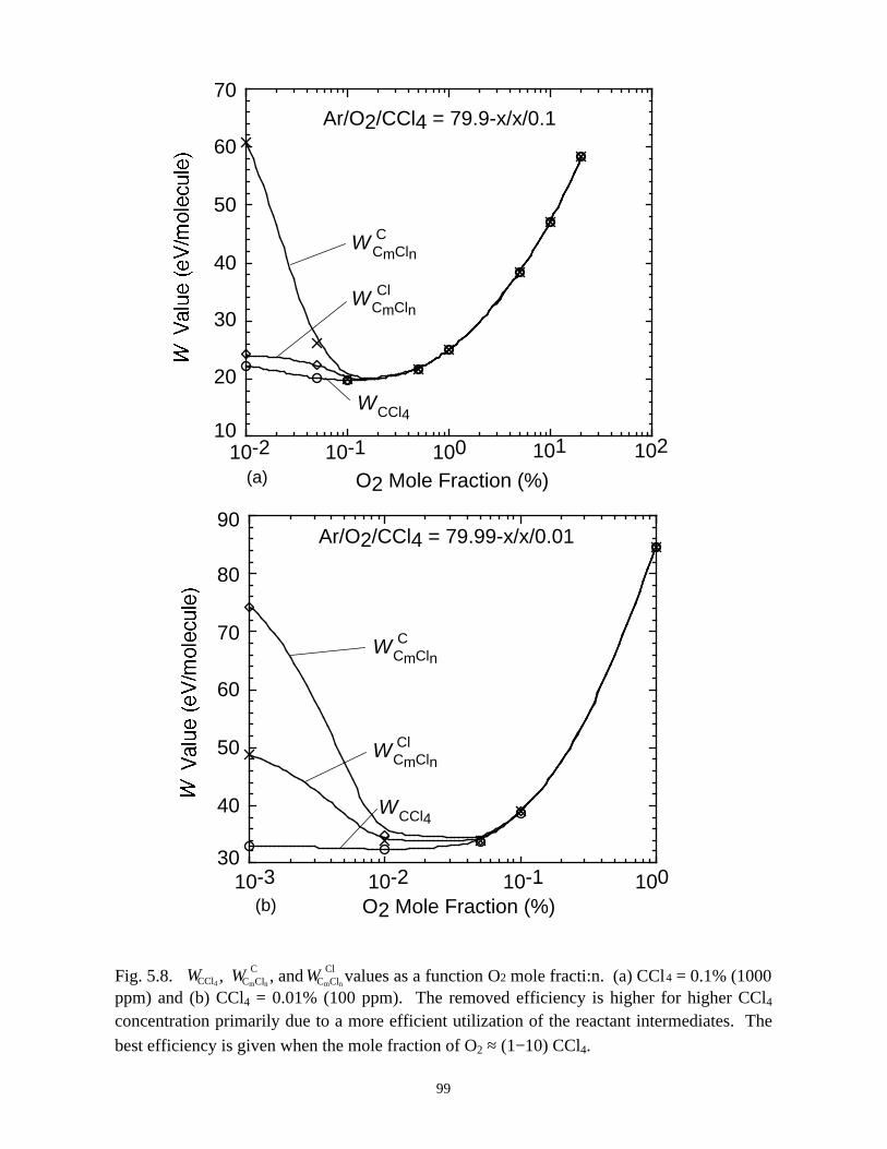
10-2 10-1 100 101 102
10-2 10-1 10010-330
40
50
60
70
80
90
30
40
50
60
70
10
20
O2 Mole Fraction (%)
O2 Mole Fraction (%)
WCmClnC
WCmClnCl
WCCl4
WCmClnC
WCmClnCl
WCCl4
Ar/O2/CCl4 = 79.9-x/x/0.1
Ar/O2/CCl4 = 79.99-x/x/0.01
Fig. 5.8. , , and values as a function O2 mole fracti:n. (a) CCl4 = 0.1% (1000ppm) and (b) CCl4 = 0.01% (100 ppm). The removed efficiency is higher for higher CCl4
concentration primarily due to a more efficient utilization of the reactant intermediates. The
best efficiency is given when the mole fraction of O2 ≈ (1−10) CCl4.
99
(a)
(b)
WCCl4 WCmClnClWCmCln
C
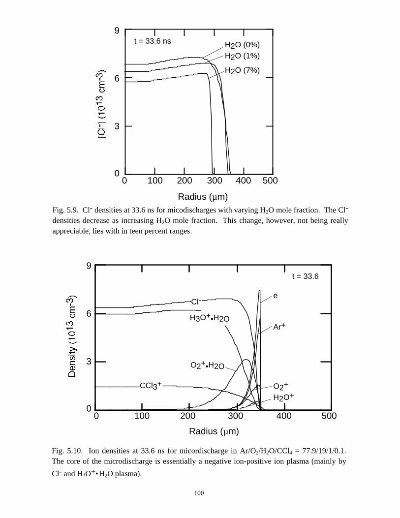
H2O (0%)H2O (1%)
H2O (7%)
3
0
6
9
Radius (µm)
0 100 400 500200 300
t = 33.6 ns
Fig. 5.9. Cl- densities at 33.6 ns for micodischarges with varying H2O mole fraction. The Cl-
densities decrease as increasing H2O mole fraction. This change, however, not being reallyappreciable, lies with in teen percent ranges.
CCl3+
Cl-
H3O+•H2O
e
Ar+
O2+
H2O+
3
0
6
9
0 100 400 500
Radius (µm)
200 300
t = 33.6
O2+•H2O
Fig. 5.10. Ion densities at 33.6 ns for micordischarge in Ar/O2/H2O/CCl4 = 77.9/19/1/0.1.The core of the microdischarge is essentially a negative ion-positive ion plasma (mainly by
Cl- and H3O+•H2O plasma).
100
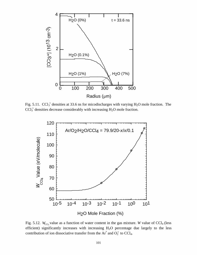
H2O (0%)
H2O (1%) H2O (7%)
2
0
4
Radius (µm)
0 100 400 500200 300
H2O (0.1%)
t = 33.6 ns
10-2 10-1 100 10110-310-410-5
110
100
50
60
70
80
90
120
H2O Mole Fraction (%)
Ar/O2/H2O/CCl4 = 79.9/20-x/x/0.1
Fig. 5.12. value as a function of water content in the gas mixture. W value of CCl4 (lessefficient) significantly increases with increasing H2O percentage due largely to the lesscontribution of ion dissociative transfer from the Ar and O2 to CCl4.
101
Fig. 5.11. CCl3 densities at 33.6 ns for micodischarges with varying H2O mole fraction. TheCCl3 densities decrease considerably with increasing H2O mole fraction.
+
+
+ +
WCCl4
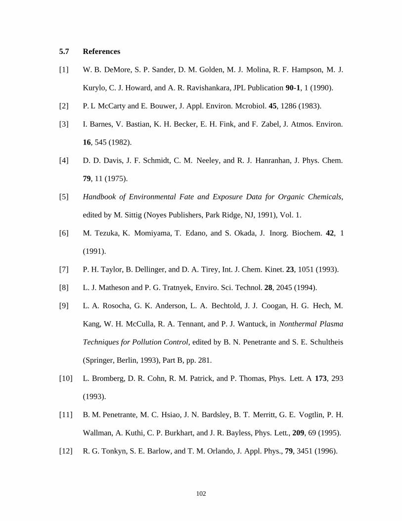
102
5.7 References
[1] W. B. DeMore, S. P. Sander, D. M. Golden, M. J. Molina, R. F. Hampson, M. J.
Kurylo, C. J. Howard, and A. R. Ravishankara, JPL Publication 90-1, 1 (1990).
[2] P. L McCarty and E. Bouwer, J. Appl. Environ. Mcrobiol. 45, 1286 (1983).
[3] I. Barnes, V. Bastian, K. H. Becker, E. H. Fink, and F. Zabel, J. Atmos. Environ.
16, 545 (1982).
[4] D. D. Davis, J. F. Schmidt, C. M. Neeley, and R. J. Hanranhan, J. Phys. Chem.
79, 11 (1975).
[5] Handbook of Environmental Fate and Exposure Data for Organic Chemicals,
edited by M. Sittig (Noyes Publishers, Park Ridge, NJ, 1991), Vol. 1.
[6] M. Tezuka, K. Momiyama, T. Edano, and S. Okada, J. Inorg. Biochem. 42, 1
(1991).
[7] P. H. Taylor, B. Dellinger, and D. A. Tirey, Int. J. Chem. Kinet. 23, 1051 (1993).
[8] L. J. Matheson and P. G. Tratnyek, Enviro. Sci. Technol. 28, 2045 (1994).
[9] L. A. Rosocha, G. K. Anderson, L. A. Bechtold, J. J. Coogan, H. G. Hech, M.
Kang, W. H. McCulla, R. A. Tennant, and P. J. Wantuck, in Nonthermal Plasma
Techniques for Pollution Control, edited by B. N. Penetrante and S. E. Schultheis
(Springer, Berlin, 1993), Part B, pp. 281.
[10] L. Bromberg, D. R. Cohn, R. M. Patrick, and P. Thomas, Phys. Lett. A 173, 293
(1993).
[11] B. M. Penetrante, M. C. Hsiao, J. N. Bardsley, B. T. Merritt, G. E. Vogtlin, P. H.
Wallman, A. Kuthi, C. P. Burkhart, and J. R. Bayless, Phys. Lett., 209, 69 (1995).
[12] R. G. Tonkyn, S. E. Barlow, and T. M. Orlando, J. Appl. Phys., 79, 3451 (1996).
103
[13] W. Niessen, O. Wolf, R. Schruft, and M. Neiger, J. Phys. D.: Appl. Phys., 31, 542
(1998).
[14] J. J. Russell, J. A. Seetula, D. Gutman, F. Danis, F, Caralp, P. D. Lightfoot, R.
Lesclaux, C. F. Melius, and S. M Senkan, J. Phys. Chem. 94, 3277 (1990).
[15] R. Atkinson, D. L. Baulch, R. A. Cox, R. F. Hampson Jr., J. A. Kerr, and J. Troe,
J. Phys. Chem. Ref. Data 21, 1125 (1992).
104
6. MODELING EXCIMER EMISSION IN DIELECTRIC BARRIERDISCHARGES
6.1 Introduction
UV radiation, with quantum energies in the range of 3-10 eV, has a number of
applications because these energetic photons are capable of splitting most chemical
bonds. Examples include sterilization [1, 2], lithography [3, 4], degradation of organic
compounds in flue gases and in water [5, 6], and UV-enhanced chemical vapor
deposition [7-9]. All of these applications require efficient UV sources of high power
that preferably radiate in a narrow selectable wavelength range. Traditional intense UV
sources, such as high-pressure mercury, Xe-arc, and flash lamps, emit in a broad spectral
range from 200 nm to several microns. Conventional narrow-bandwidth UV sources
such as low-pressure mercury and rare-gases resonance-line lamps have small UV
intensities. Though excimer lasers can be used as sources of intense narrow-bandwidth
UV radiation, they are expensive in capital and operating costs, and provide only a small
beam. In addition, incoherent UV sources have shown other advantages over UV lasers
in photodeposition for metal, dielectric, or semiconductor layers [7, 10, 11]. For example
incoherent excimer UV sources produced smooth continuous films while excimer laser
deposition resulted in discontinuous grainy Pd films [7].
Excimers are bound excited states of molecules that do not have a stable molecule
ground state. There are a number of methods for generating excimers, such as dielectric
barrier discharges, coronas, high-energy beams, x-rays, α-particles, protons, heavy ions,
synchrotron radiation, and microwave discharges [12-18]. Of these, DBDs are
potentially more attractive due to their simplicity, stability, low cost, high power, and
105
easy maintenance. Depending on the gas mixture, many different excimers could be
generated in dielectric barrier discharges, which include rare gas dimers such as Ar2* (126
nm), Kr2* (146 nm), and Xe2
* (172 nm), rare gas-halide complex such as ArF* (193 nm),
KrF* (249 nm), XeF* (354 nm), ArCl* (175 nm), KrCl* (222 nm), XeCl* (308 nm), ArBr*
(165 nm), KrBr* (207 nm), XeBr* (283 nm), KrI* (190 nm), and XeI* (253 nm), and
halogen dimers such as F2* (158 nm), Cl2
* (259 nm), Br2* (289), and I2
* (342 nm) [19-26].
Each emits radiation in a narrow wavelength band of the vacuum ultraviolet (VUV) or
UV part of the spectrum.
In this chapter, the dynamics of generating radiation and excimer formation for
mixtures of chlorine and xenon gases in dielectric barrier discharges will be discussed.
The 1-D PCHM has been used to determine operating parameters that optimize the
efficiency of generating examer radiation. Section 6.2 is an overview of the formation of
excimers in Xe/Cl2 mixtures. In Section 6.3, we present the microdischarge dynamics
and the spatial dependencies of excimer and photon generation. We discuss the
optimization of discharge conditions for excimer and photon generation in Section 6.4.
Concluding remarks are in Section 6.5.
6.2 Formation of Excimers
The dominant reaction pathways for generating the major four excimers, XeCl* (λ
= 308 nm), Xe2* (λ = 172 nm), Xe2Cl* (λ = 490 nm), and Cl2
* (λ = 259 nm) in Xe/Cl2
mixtures are shown in Fig. 6.1. Species and reaction rate coefficients for these and other
processes are listed in Appendices A and B. Among these excited species, XeCl* is
expected to be the primary excimer for Xe/Cl2 gas mixtures. A simplified potential
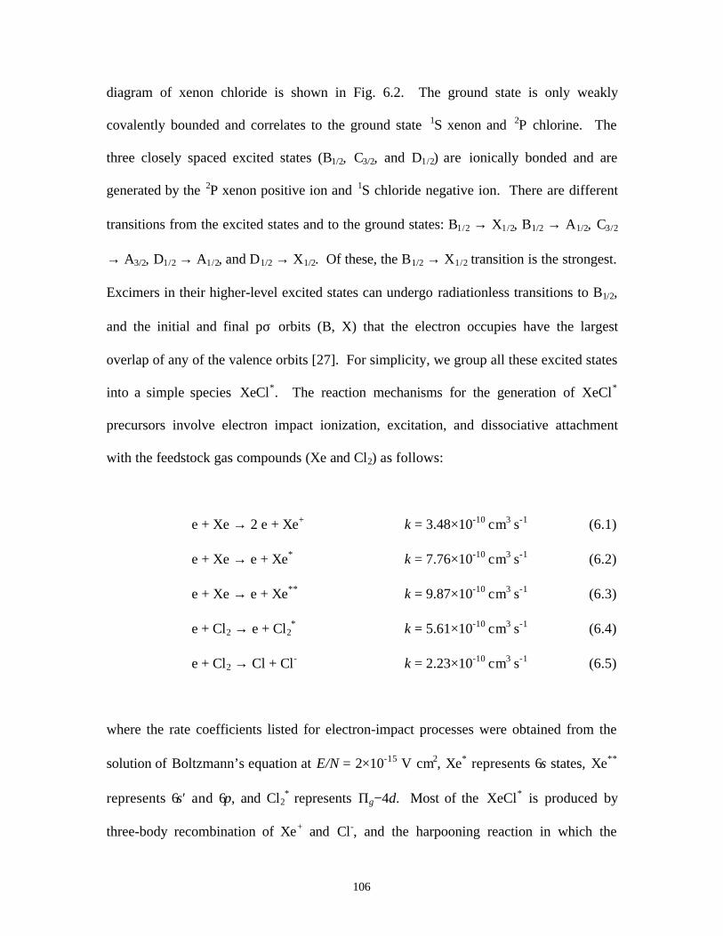
106
diagram of xenon chloride is shown in Fig. 6.2. The ground state is only weakly
covalently bounded and correlates to the ground state 1S xenon and 2P chlorine. The
three closely spaced excited states (B1/2, C3/2, and D1/2) are ionically bonded and are
generated by the 2P xenon positive ion and 1S chloride negative ion. There are different
transitions from the excited states and to the ground states: B1/2 → X1/2, B1/2 → A1/2, C3/2
→ A3/2, D1/2 → A1/2, and D1/2 → X1/2. Of these, the B1/2 → X1/2 transition is the strongest.
Excimers in their higher-level excited states can undergo radiationless transitions to B1/2,
and the initial and final pσ orbits (B, X) that the electron occupies have the largest
overlap of any of the valence orbits [27]. For simplicity, we group all these excited states
into a simple species XeCl*. The reaction mechanisms for the generation of XeCl*
precursors involve electron impact ionization, excitation, and dissociative attachment
with the feedstock gas compounds (Xe and Cl2) as follows:
e + Xe → 2 e + Xe+ k = 3.48×10⁻¹⁰ cm3 s-1 (6.1)
e + Xe → e + Xe* k = 7.76×10⁻¹⁰ cm3 s-1 (6.2)
e + Xe → e + Xe** k = 9.87×10⁻¹⁰ cm3 s-1 (6.3)
e + Cl2 → e + Cl2* k = 5.61×10⁻¹⁰ cm3 s-1 (6.4)
e + Cl2 → Cl + Cl- k = 2.23×10⁻¹⁰ cm3 s-1 (6.5)
where the rate coefficients listed for electron-impact processes were obtained from the
solution of Boltzmann’s equation at E/N = 2×10-15 V cm2, Xe* represents 6s states, Xe**
represents 6s′ and 6p, and Cl2* represents Πg−4d. Most of the XeCl* is produced by
three-body recombination of Xe+ and Cl-, and the harpooning reaction in which the
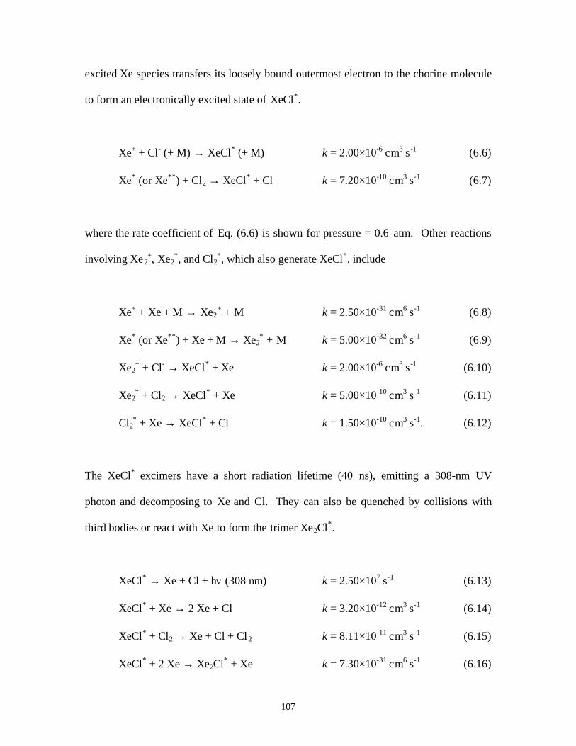
107
excited Xe species transfers its loosely bound outermost electron to the chorine molecule
to form an electronically excited state of XeCl*.
Xe+ + Cl- (+ M) → XeCl* (+ M) k = 2.00×10⁻⁶ cm3 s-1 (6.6)
Xe* (or Xe**) + Cl2 → XeCl* + Cl k = 7.20×10⁻¹⁰ cm3 s-1 (6.7)
where the rate coefficient of Eq. (6.6) is shown for pressure = 0.6 atm. Other reactions
involving Xe2+, Xe2
*, and Cl2*, which also generate XeCl*, include
Xe+ + Xe + M → Xe2+ + M k = 2.50×10⁻³¹ cm6 s-1 (6.8)
Xe* (or Xe**) + Xe + M → Xe2* + M k = 5.00×10⁻³² cm6 s-1 (6.9)
Xe2+ + Cl- → XeCl* + Xe k = 2.00×10⁻⁶ cm3 s-1 (6.10)
Xe2* + Cl2 → XeCl* + Xe k = 5.00×10⁻¹⁰ cm3 s-1 (6.11)
Cl2* + Xe → XeCl* + Cl k = 1.50×10⁻¹⁰ cm3 s-1. (6.12)
The XeCl* excimers have a short radiation lifetime (40 ns), emitting a 308-nm UV
photon and decomposing to Xe and Cl. They can also be quenched by collisions with
third bodies or react with Xe to form the trimer Xe2Cl*.
XeCl* → Xe + Cl + hν (308 nm) k = 2.50×10⁷ s-1 (6.13)
XeCl* + Xe → 2 Xe + Cl k = 3.20×10⁻¹² cm3 s-1 (6.14)
XeCl* + Cl2 → Xe + Cl + Cl2 k = 8.11×10⁻¹¹ cm3 s-1 (6.15)
XeCl* + 2 Xe → Xe2Cl* + Xe k = 7.30×10⁻³¹ cm6 s-1 (6.16)
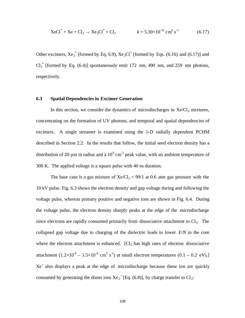
108
XeCl* + Xe + Cl2 → Xe2Cl* + Cl2 k = 5.30×10⁻³¹ cm6 s-1 (6.17)
Other excimers, Xe2* (formed by Eq. 6.9), Xe2Cl* [formed by Eqs. (6.16) and (6.17)] and
Cl2* [formed by Eq. (6.4)] spontaneously emit 172 nm, 490 nm, and 259 nm photons,
respectively.
6.3 Spatial Dependencies in Excimer Generation
In this section, we consider the dynamics of microdischarges in Xe/Cl2 mixtures,
concentrating on the formation of UV photons, and temporal and spatial dependencies of
excimers. A single streamer is examined using the 1-D radially dependent PCHM
described in Section 2.2. In the results that follow, the initial seed electron density has a
distribution of 20 µm in radius and a 109 cm-3 peak value, with an ambient temperature of
300 K. The applied voltage is a square pulse with 40 ns duration.
The base case is a gas mixture of Xe/Cl2 = 99/1 at 0.6 atm gas pressure with the
10 kV pulse. Fig. 6.3 shows the electron density and gap voltage during and following the
voltage pulse, whereas primary positive and negative ions are shown in Fig. 6.4. During
the voltage pulse, the electron density sharply peaks at the edge of the microdischarge
since electrons are rapidly consumed primarily from dissociative attachment to Cl2. The
collapsed gap voltage due to charging of the dielectric leads to lower E/N in the core
where the electron attachment is enhanced. [Cl2 has high rates of electron dissociative
attachment (1.2×10⁻⁹ – 1.5×10⁻⁹ cm3 s-1) at small electron temperatures (0.1 – 0.2 eV).]
Xe+ also displays a peak at the edge of microdischarge because these ion are quickly
consumed by generating the dimer ions Xe2+ [Eq. (6.8)], by charge transfer to Cl2:
109
Xe+ + Cl2 → Xe + Cl2+ k = 6.0×10⁻¹¹ cm3 s-1 (6.18)
and by the three-body recombination with Cl-. The Xe2+ and Cl- density profiles display
a less sharp edge than those of Xe+ and electrons, while the Cl2+ density shows a steady
decrease with increasing radius.
The neutral excited species Xe* and Xe**, which are precursors to the generation
of XeCl*, also have sharp edges (as does the Xe+) and have approximately the same
densities, as shown in Fig. 6.5. These species are lost primarily by radiative relaxation
(Xe* → Xe, k = 3.93×10⁶ s-1; Xe** → Xe, k = 3.0×10⁷ s-1), harpooning reactions [Eq.
(6.7)], dimerzation (Eq. 6.9) and Penning ionization:
Xe* (or Xe**) + Cl2 → Xe + Cl2+ k = 5.0×10⁻¹⁰ cm3 s-1. (6.19)
The behavior of XeCl* and its corresponding photon generation at 308 nm are
shown in Fig. 6.6. The formation of the XeCl* excimer is delayed compared to electron
generation due to there being two or three steps required for its formation. The total
generation of 308-nm photons is ultimately uniform across the microdischarge. The
emissions of other photons (172 nm, 490 nm, and 259 nm emitted by Xe2*, Xe2Cl*, and
Cl2* respectively) are shown in Fig. 6.7. The distribution of the total number of these
photons appears fairly uniform across the entire microdischarge. The ratios of the total
number of 308-nm photons to those at 172 nm, 490 nm, and 259 nm photons are 2.63,
0.99, and 6075.4 respectively. In addition, Xe2Cl* displays a long lifetime since its
110
quenching rate is nearly independent of the Xe pressure and only dependent on the Cl2
density [28]. Cl2* has a short lifetime due to a quick consumption by conversion to
XeCl*, and Xe2* has a lifetime similar to XeCl*.
Electron attachment significantly increases with increasing Cl2 mole fraction. As
a result, the dynamics of the microdischarge can be changed. The results for Xe/Cl2 =
95/5 with otherwise the same conditions as the base case are shown in Figs. 6.8-6.10.
The electron density and gap voltage for different times are shown in Fig. 6.8. The
electron density in the core is driven to such a low value during the pulse that there is not
an immediate second avalanche in the core at the end of pulse. Instead, after the pulse,
the electron density shell propagates towards the center of the microdischarge due to
there being high gap voltages in the core. XeCl* and 308-nm photons are regenerated in
the core as the second avalanche moves towards the center, as shown in Fig. 6.9. The
total number of 308 nm photons is slightly lower than the base case. However, the
generation of 172 nm (Xe2*) and 490 nm (Xe2Cl*) photons dramatically decreases and
the generation of 259 nm photons increases compared to the Xe/Cl2 =99/1 case, as shown
in Fig. 6.10. This trend is due to the fact that Cl2 is very efficient at quenching Xe 2* and
Xe2Cl*, and the higher Cl2 mole fraction is beneficial to generating Cl2*.
6.4 Optimization of Discharge Conditions for Excimer and Photon Generation
The efficiency of UV photon generation in DBDs depends on the dielectric
properties, gas composition, gas pressure, and applied voltage. In this section, we
describe the consequences of varying these factors for Xe/Cl2 gas mixtures. In the
following discussion, the base case from the last section is used as a starting point. The
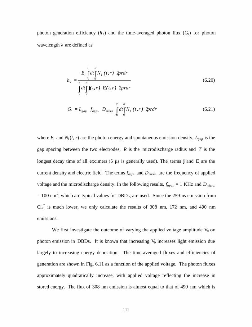
111
photon generation efficiency (ηλ) and the time-averaged photon flux (Γλ) for photon
wavelength λ are defined as
∫∫
∫ ∫
⋅⋅
⋅=
RT
T R
rdrrtrtdt
rdrrtNdtE
00
0 0
2
2
π
πη
λλ
λ
),(),(
),(
Ej
(6.20)
rdrrtNdtDfLT R
microapplgap πΓ λλ ∫ ∫ ⋅⋅⋅⋅=0 0
2),(. (6.21)
where Eλ and Nλ(t, r) are the photon energy and spontaneous emission density, Lgap is the
gap spacing between the two electrodes, R is the microdischarge radius and T is the
longest decay time of all excimers (5 µs is generally used). The terms j and E are the
current density and electric field. The terms fappl. and Dmicro. are the frequency of applied
voltage and the microdischarge density. In the following results, fappl. = 1 KHz and Dmicro.
= 100 cm-2, which are typical values for DBDs, are used. Since the 259-ns emission from
Cl2* is much lower, we only calculate the results of 308 nm, 172 nm, and 490 nm
emissions.
We first investigate the outcome of varying the applied voltage amplitude V0 on
photon emission in DBDs. It is known that increasing V0 increases light emission due
largely to increasing energy deposition. The time-averaged fluxes and efficiencies of
generation are shown in Fig. 6.11 as a function of the applied voltage. The photon fluxes
approximately quadratically increase, with applied voltage reflecting the increase in
stored energy. The flux of 308 nm emission is almost equal to that of 490 nm which is
112
coincidental and not “physics.” When the applied voltage magnitude is increased, a
higher fraction of power deposition goes into producing excitation and ionization. As a
result, the efficiencies of 308 nm and 490 nm generations improve at higher applied
voltage. However the efficiency of 172 nm generation has a weaker dependence on the
applied voltage since increasing it is rapidly quenched by reactions such as with Cl2.
The consequences of dielectric capacitance (εd/L, where εd = permittivity and L =
thickness of the dielectric) on the photon emission fluxes and photon generation
efficiencies are shown in Fig. 6.12. With a larger dielectric capacitance, more current is
required to charge the dielectric. Therefore, more energy is deposited in the plasma and
the corresponding photon fluxes are larger [Fig. 6.12(a)].
The effect of Cl2 mole fraction on the photon fluxes and generation efficiency are
shown in Fig. 6.13. When the Cl2 mole fraction is larger than 1%, the generation of 308
nm photons is dominant. There is an optimum efficiency for 308 nm generation at Cl2 ≈
1%. Increasing Cl2 concetration enhances the ion transfer reaction from Xe+ to Cl2 [Eq.
(6.18)], which results in consuming more Xe+, but leads to an increase of Cl- generation.
Both Xe+ and Cl- are important precursors forming XeCl* [via Eq. (6.6)]. However, the
fluxes and generation efficiency for 172 nm and 490 nm photons strongly decrease with
increasing Cl2, since Cl2 can efficiently quench Xe 2* and Xe2Cl*.
We also investigated the consequences of gas pressure on the photon fluxes and
efficiencies at the same initial (E/N)0 = 3.4×10⁻¹⁵ V cm2 as shown in Fig. 6.14. The
emissions of three photons increase with increasing gas pressure due to higher gas
density resulting in more UV emission. The efficiencies of 308 nm and 490 nm photon
generation are improved at low pressures due to decreased quenching. However the
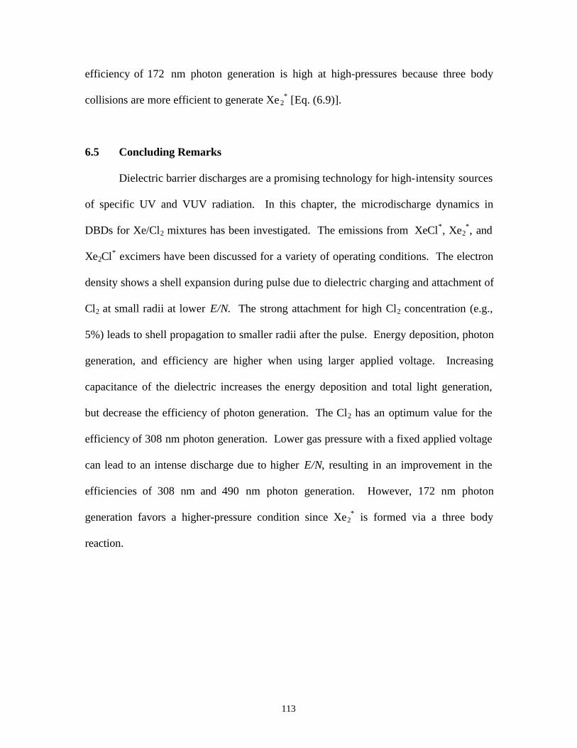
113
efficiency of 172 nm photon generation is high at high-pressures because three body
collisions are more efficient to generate Xe2* [Eq. (6.9)].
6.5 Concluding Remarks
Dielectric barrier discharges are a promising technology for high-intensity sources
of specific UV and VUV radiation. In this chapter, the microdischarge dynamics in
DBDs for Xe/Cl2 mixtures has been investigated. The emissions from XeCl*, Xe2*, and
Xe2Cl* excimers have been discussed for a variety of operating conditions. The electron
density shows a shell expansion during pulse due to dielectric charging and attachment of
Cl2 at small radii at lower E/N. The strong attachment for high Cl2 concentration (e.g.,
5%) leads to shell propagation to smaller radii after the pulse. Energy deposition, photon
generation, and efficiency are higher when using larger applied voltage. Increasing
capacitance of the dielectric increases the energy deposition and total light generation,
but decrease the efficiency of photon generation. The Cl2 has an optimum value for the
efficiency of 308 nm photon generation. Lower gas pressure with a fixed applied voltage
can lead to an intense discharge due to higher E/N, resulting in an improvement in the
efficiencies of 308 nm and 490 nm photon generation. However, 172 nm photon
generation favors a higher-pressure condition since Xe2* is formed via a three body
reaction.
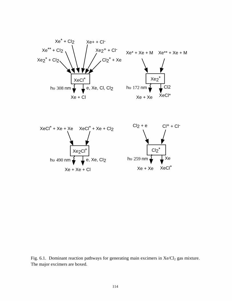
Xe2* + Cl2
XeCl*
Xe+ + Cl-Xe* + Cl2
Xe** + Cl2 Xe2+ + Cl-
Cl2* + Xe
hυ 308 nm
Xe + Cl
e, Xe, Cl, Cl2
Xe* + Xe + M Xe** + Xe + M
Xe2*
hυ 172 nm
Xe + Xe
Cl2
XeCl*
XeCl* + Xe + Xe XeCl* + Xe + Cl2
Xe2Cl*
hυ 490 nm
Xe + Xe + Cl
e, Xe, Cl2
Cl2*
Cl2 + e Cl+ + Cl-
hυ 259 nm
Xe + Xe
Xe
XeCl*
Fig. 6.1. Dominant reaction pathways for generating main excimers in Xe/Cl2 gas mixture.The major excimers are boxed.
114
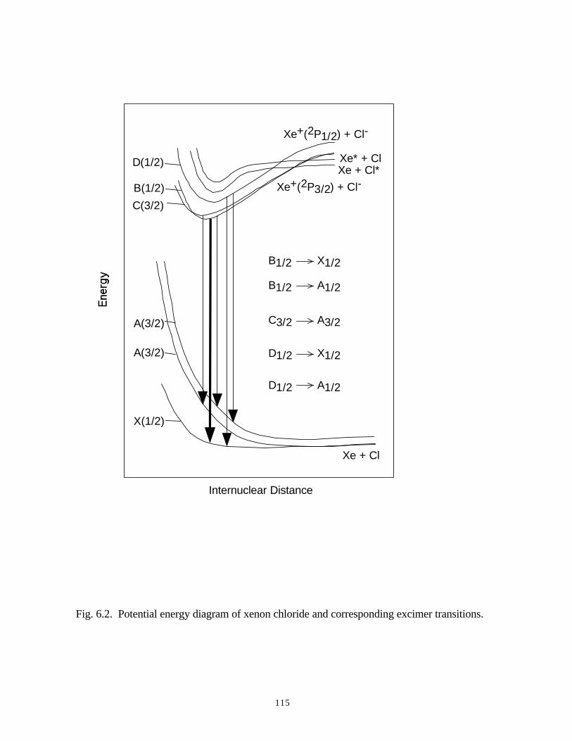
B1/2 X1/2
X(1/2)
A(3/2)
B(1/2)
C(3/2)
D(1/2)
Internuclear Distance
Xe+(2P3/2) + Cl-
Xe+(2P1/2) + Cl-
Xe* + ClXe + Cl*
Xe + Cl
A(3/2)
B1/2 A1/2
C3/2 A3/2
D1/2 X1/2
D1/2 A1/2
Fig. 6.2. Potential energy diagram of xenon chloride and corresponding excimer transitions.
115
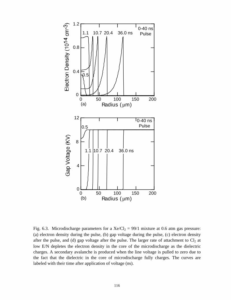
0
0.4
0.8
1.2
0.5
1.1 10.7 36.0 ns20.4
0.5
1.1 10.7 36.0 ns
0
4
8
12
20.4
0 50 100 150 200Radius (µm)
0 50 100 150 200Radius (µm)
Fig. 6.3. Microdischarge parameters for a Xe/Cl2 = 99/1 mixture at 0.6 atm gas pressure:(a) electron density during the pulse, (b) gap voltage during the pulse, (c) electron densityafter the pulse, and (d) gap voltage after the pulse. The larger rate of attachment to Cl2 atlow E/N depletes the electron density in the core of the microdischarge as the dielectriccharges. A secondary avalanche is produced when the line voltage is pulled to zero due tothe fact that the dielectric in the core of microdischarge fully charges. The curves arelabeled with their time after application of voltage (ns).
116
0-40 nsPulse
(a)
0-40 nsPulse
(b)
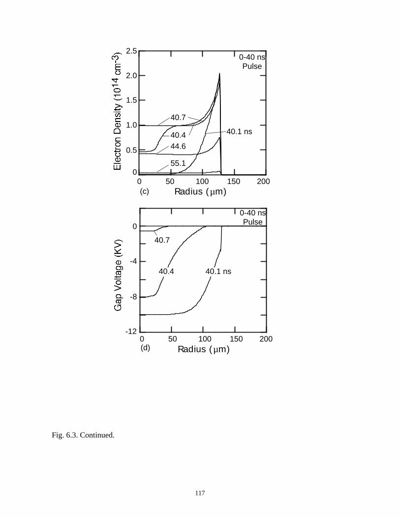
0
0.5
1.0
1.5
2.0
2.5
40.4
40.7
44.6
55.1
40.1 ns
0 50 100 150 200
40.1 ns40.4
40.7
-12
-8
-4
0
Radius (µm)
0 50 100 150 200Radius (µm)
Fig. 6.3. Continued.
117
0-40 nsPulse
(c)
0-40 nsPulse
(d)
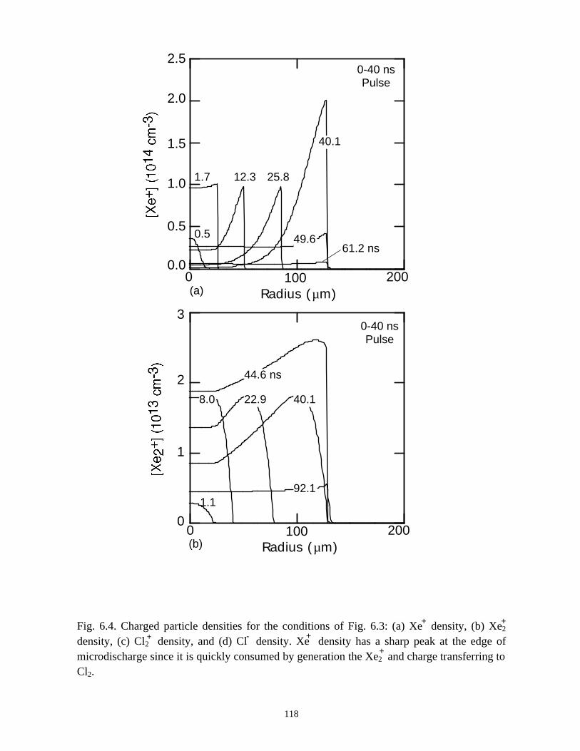
0.5 49.6
12.3
40.1
25.81.7
61.2 ns
0.0
0.5
1.0
1.5
0 100 200Radius (µm)
2.0
2.5
1.1
8.0 22.9 40.1
44.6 ns
92.1
0 100 200Radius (µm)
1
0
2
3
0-40 nsPulse
(a)
0-40 nsPulse
(b)
Fig. 6.4. Charged particle densities for the conditions of Fig. 6.3: (a) Xe density, (b) Xe2
density, (c) Cl2 density, and (d) Cl density. Xe density has a sharp peak at the edge ofmicrodischarge since it is quickly consumed by generation the Xe2 and charge transferring toCl2.
118
+
+ +
+ -
+
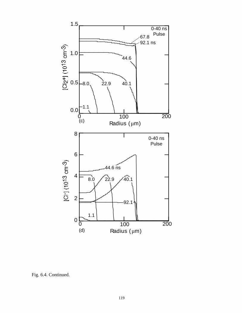
1.1
8.0 22.9 40.1
44.6 ns
0 100 200Radius (µm)
2
0
6
8
4
92.1
1.1
8.0 22.9 40.1
44.6
92.1 ns67.8
0.0
0.5
1.0
1.5
0 100 200Radius (µm)
0-40 nsPulse
(c)
Fig. 6.4. Continued.
119
0-40 nsPulse
(d)
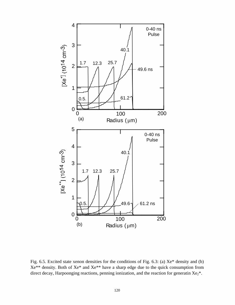
1.7 12.3
40.1
61.2
0 100 200Radius (µm)
1
0
3
4
2
0.5.
25.7
49.6 ns
0 100 200Radius (µm)
1
0
3
4
2
5
1.7 12.3
40.1
61.2 ns0.5.
25.7
49.6
Fig. 6.5. Excited state xenon densities for the conditions of Fig. 6.3: (a) Xe* density and (b)Xe** density. Both of Xe* and Xe** have a sharp edge due to the quick consumption fromdirect decay, Harpoonging reactions, penning ionization, and the reaction for generatin Xe2*.
120
0-40 nsPulse
(a)
0-40 nsPulse
(b)
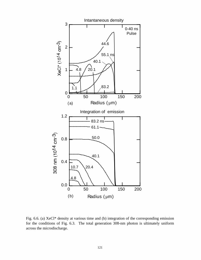
Radius (µm)(a)
1.1
4.8 20.1
40.1
44.6
55.1 ns
83.2
0
1
2
3
0 50 100 150 200
Intantaneous density
(b) Radius (µm)
Integration of emission
4.8
10.7 20.4
40.1
50.0
83.2 ns
0.0
0.4
0.8
1.2
0 50 100 150 200
61.1
Fig. 6.6. (a) XeCl* density at various time and (b) integration of the corresponding emissionfor the conditions of Fig. 6.3. The total generation 308-nm photon is ultimately uniformacross the microdischarge.
121
0-40 nsPulse
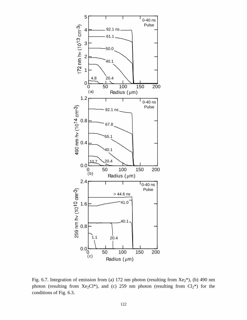
Radius (µm)
4.8 20.4
40.1
50.0
92.1 ns
61.1
0 50 100 150 2000
1
2
3
4
5
10.7 20.4
40.1
55.1
92.1 ns
67.8
0.0
0.4
0.8
1.2
0 50 100 150 200
0.0
0.8
1.6
2.4
0 50 100 150 200
Radius (µm)
Radius (µm)
20.4
40.1
> 44.6 ns
41.0
1.1
(a)
0-40 nsPulse
(b)
0-40 nsPulse
(c)
0-40 nsPulse
Fig. 6.7. Integration of emission from (a) 172 nm photon (resulting from Xe2*), (b) 490 nmphoton (resulting from Xe2Cl*), and (c) 259 nm photon (resulting from Cl2*) for theconditions of Fig. 6.3.
122
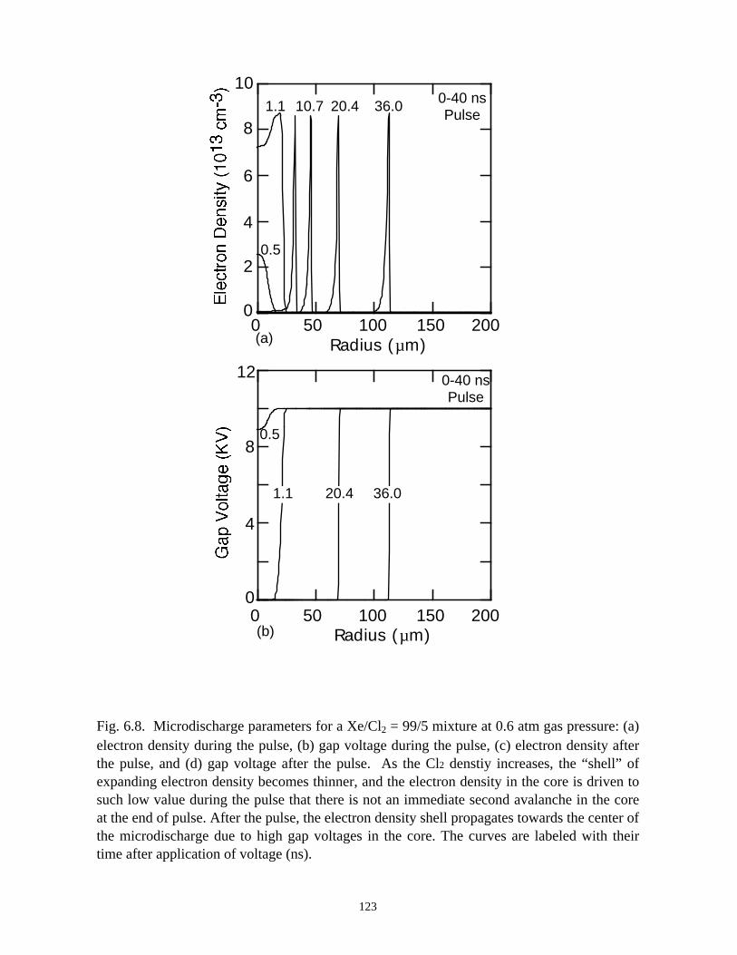
0 50 100 150 200
0.5
1.1 20.4 36.0
0
12
4
8
0.5
1.1 10.7 36.020.4
2
4
6
8
10
0
Radius (µm)
Radius (µm)
0 50 100 150 200
Fig. 6.8. Microdischarge parameters for a Xe/Cl2 = 99/5 mixture at 0.6 atm gas pressure: (a)electron density during the pulse, (b) gap voltage during the pulse, (c) electron density afterthe pulse, and (d) gap voltage after the pulse. As the Cl2 denstiy increases, the “shell” ofexpanding electron density becomes thinner, and the electron density in the core is driven tosuch low value during the pulse that there is not an immediate second avalanche in the coreat the end of pulse. After the pulse, the electron density shell propagates towards the center ofthe microdischarge due to high gap voltages in the core. The curves are labeled with theirtime after application of voltage (ns).
123
0-40 nsPulse
(a)
0-40 nsPulse
(b)
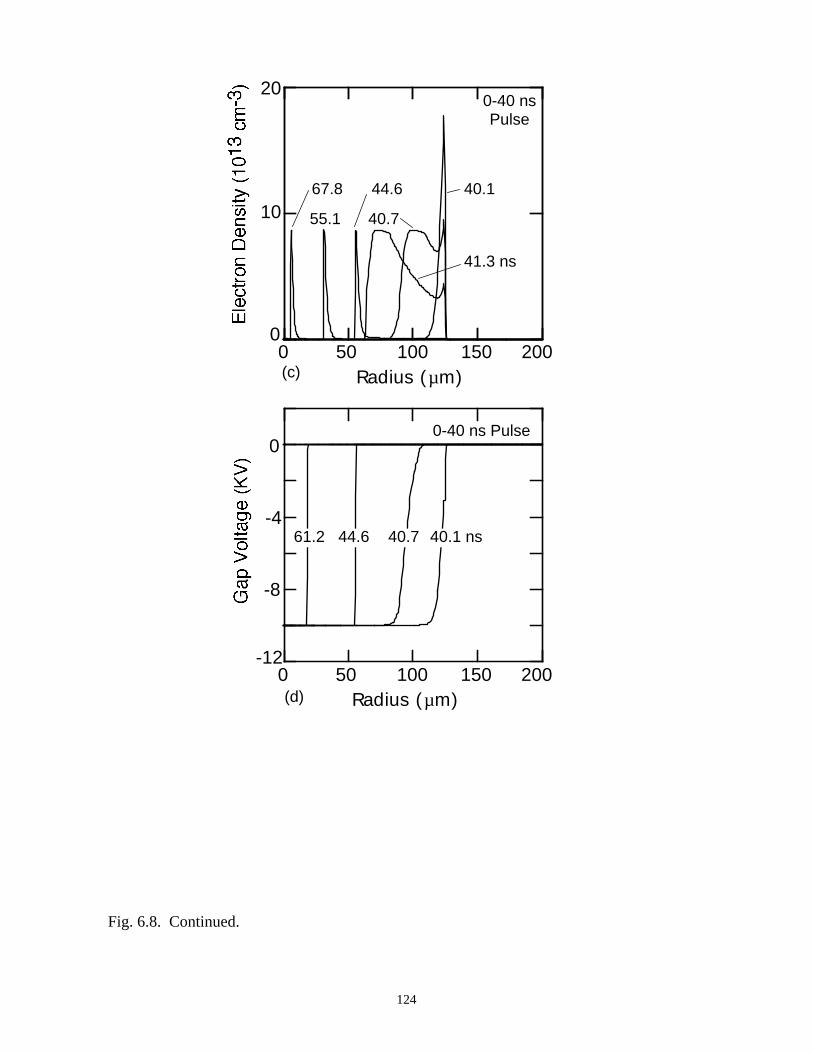
40.1 ns40.744.661.2
0 50 100 150 200-12
0
-4
-8
40.144.6
55.1
67.8
40.7
41.3 ns
20
10
0
Radius (µm)
0 50 100 150 200Radius (µm)(c)
(d)
0-40 ns Pulse
0-40 nsPulse
Fig. 6.8. Continued.
124
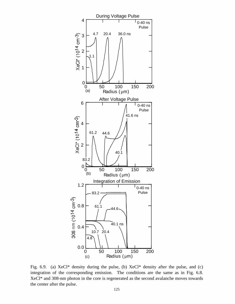
Radius (µm)
1.1
36.0 ns20.44.7
0 50 100 150 200
4
0
2
3
1
During Voltage Pulse
Radius (µm)
40.1
41.6 ns
44.661.2
83.2
0 50 100 150 200
4
0
2
6After Voltage Pulse
4.8
10.7 20.4
40.1 ns
44.6
83.2
61.1
0.0
0.4
0.8
1.2
0 50 100 150 200
Integration of Emission
Radius (µm)
0-40 nsPulse
(a)
0-40 nsPulse
(b)
0-40 nsPulse
(c)
Fig. 6.9. (a) XeCl* density during the pulse, (b) XeCl* density after the pulse, and (c)integration of the corresponding emission. The conditions are the same as in Fig. 6.8.XeCl* and 308-nm photon in the core is regenerated as the second avalanche moves towardsthe center after the pulse.
125
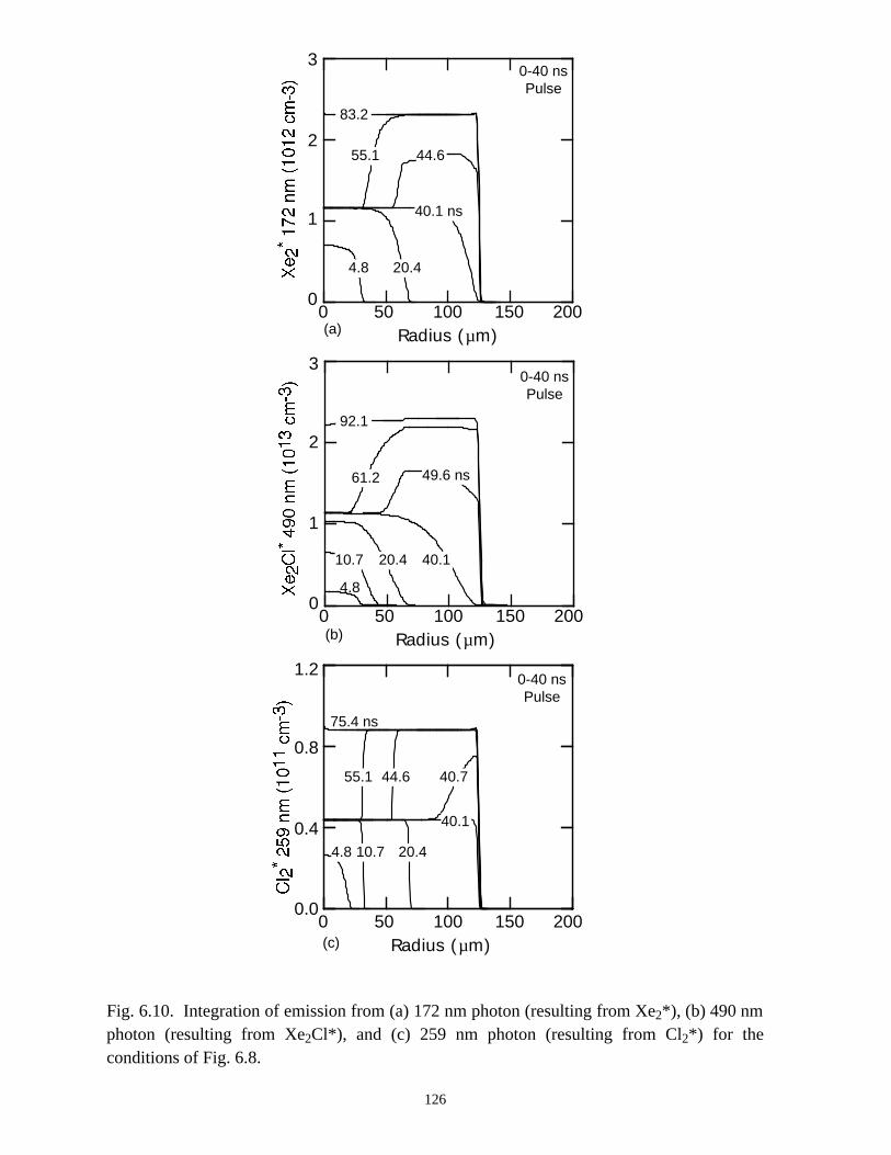
Radius (µm)
4.8 20.4
40.1 ns
44.6
83.2
55.1
0 50 100 150 2000
1
2
3
Radius (µm)
4.8
20.4 40.1
49.6 ns
92.1
61.2
0 50 100 150 2000
1
2
3
10.7
Radius (µm)0 50 100 150 200
0.0
0.4
0.8
1.2
4.8 10.7 20.4
40.1
44.6
75.4 ns
55.1 40.7
0-40 nsPulse
(a)
0-40 nsPulse
(b)
0-40 nsPulse
(c)
Fig. 6.10. Integration of emission from (a) 172 nm photon (resulting from Xe2*), (b) 490 nmphoton (resulting from Xe2Cl*), and (c) 259 nm photon (resulting from Cl2*) for theconditions of Fig. 6.8.
126
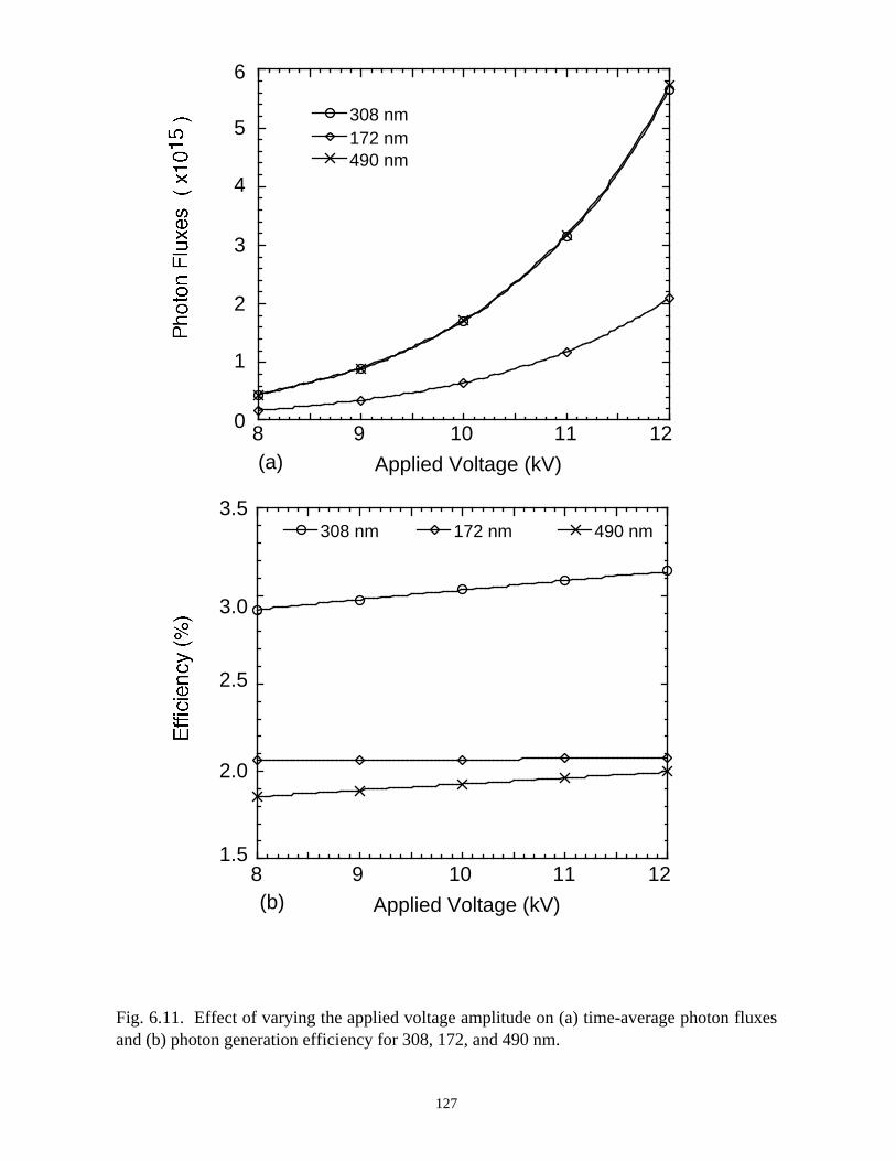
308 nm172 nm490 nm
308 nm 172 nm 490 nm
8 9 10 11 12
Applied Voltage (kV)
0
1
2
3
4
5
6
8 9 10 11 12
Applied Voltage (kV)
1.5
2.0
2.5
3.0
3.5
Fig. 6.11. Effect of varying the applied voltage amplitude on (a) time-average photon fluxesand (b) photon generation efficiency for 308, 172, and 490 nm.
127
(a)
(b)
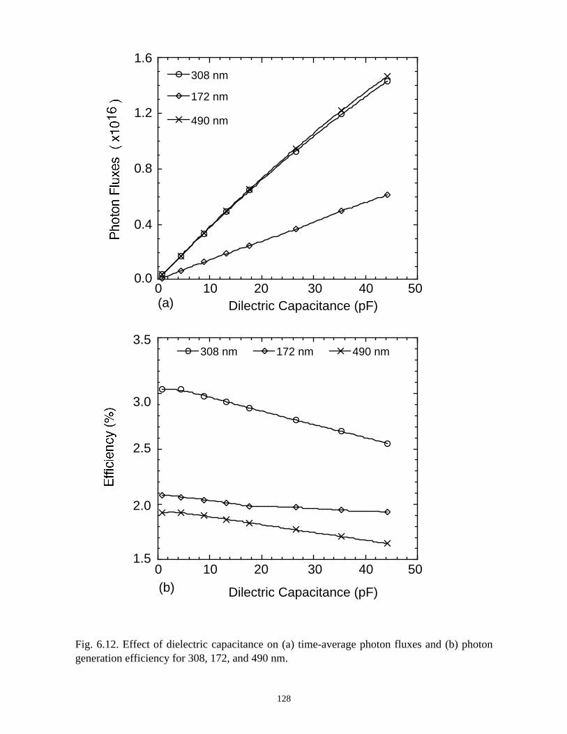
308 nm
172 nm
490 nm
308 nm 172 nm 490 nm
1.5
2.0
2.5
3.0
3.5
0 10 20 30 40
Dilectric Capacitance (pF)
50
Dilectric Capacitance (pF)0 10 20 30 40 50
0.0
0.4
0.8
1.2
1.6
Fig. 6.12. Effect of dielectric capacitance on (a) time-average photon fluxes and (b) photongeneration efficiency for 308, 172, and 490 nm.
128
(a)
(b)
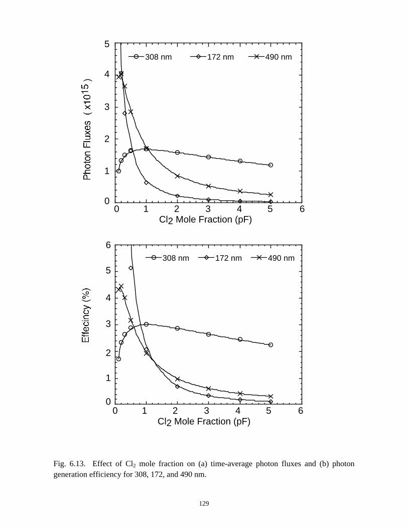
Fig. 6.13. Effect of Cl2 mole fraction on (a) time-average photon fluxes and (b) photongeneration efficiency for 308, 172, and 490 nm.
129
308 nm 172 nm 490 nm
308 nm 172 nm 490 nm
3
0
1
2
Cl2 Mole Fraction (pF)0 1 2 3 4 5 6
Cl2 Mole Fraction (pF)0 1 2 3 4 5 6
0
2
4
6
1
3
5
4
5
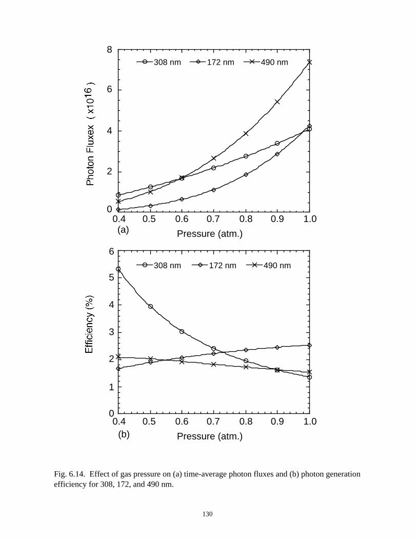
308 nm 172 nm 490 nm
308 nm 172 nm 490 nm
6
0
4
8
Pressure (atm.)
0.4 0.5 0.6 0.7 0.8 0.9 1.00
2
4
6
1
3
5
Pressure (atm.)
0.4 0.5 0.6 0.7 0.8 0.9 1.0
Fig. 6.14. Effect of gas pressure on (a) time-average photon fluxes and (b) photon generationefficiency for 308, 172, and 490 nm.
130
(a)
(b)
2
131
6.6 References
[1] A. M. Braun, M. T. Maurette, E. Oliveros, Photochemical Technology (John
Wiley, New York, 1991).
[2] R. F. Scheir and B. F. Fencl, Heat. Pip. Air Cond. J. 68, 109 (1996).
[3] D. J. Elliott, Microlithography: Process Technology for IC Fabrication (New
York : McGraw-Hill, 1986).
[4] D. Collier and W. Pantley, Laser Focus World 34, 63 (1998).
[5] H. Scheytt, H. Esron, L. Prager, R. Mehnert, and C. von Sonntag, in Proceedings
of the NATO Advanced Research Workshop on Non-Thermal Plasma Techniques
for Pollution Control, Part B, edited by P. Penetrante and S. Schulthesis
(Springer-Verlag, Berlin, 1993) pp. 91-101.
[6] O. Legrini, E. Oliveros, and A. M. Braun, Chem. Rev. 93, 671 (1993).
[7] U. Kogelschatz, Appl. Surf. Sci. 54, 410 (1992).
[8] M. E. Gross, A. Appelbaum, and P. K. Gallagher, J. Appl. Phys. 61, 1628 (1987).
[9] H. Esrom and U. Kogelschatz, Mater. Res. Soc. Symp. Proc. 158, 189 (1990).
[10] H. Esrom, J. Demny, and U. Kogelschatz, Chemtronics, 4, 202 (1989).
[11] T. H. Baum, J. Electrochem. Soc. 137, 252 (1990).
[12] B. Eliasson and U. Kogelschatz, IEEE Trans. Plasma Sci. 19, 309 (1991).
[13] H. A. Koehler, L. J Ferderber, D. L. Redhead, and P. J. Ebert, Phy. Rev. A 9, 768
(1974)
[14] O. Dutuit, R. A. Gutchek, and J. Lecalve, Chem. Phys. Lett. 58, 66 (1978).
[15] M. Kitamura, K. Mitsuka, and H. Sato, Appl. Surf. Sci. 79/80, 507 (1994).
[16] T. Gerber, W. Luethy, and P. Burkhard, Opt. Commun. 35, 242 (1980).
132
[17] W. Wieme, J. Lenaerts, J. Chem . Phys. 74, 483 (1981).
[18] D. J. Eckstrom, H. H. Nakano, D. C. Lorents, T. Rothem, J. A. Betts, M. Lainhart,
K. J. Triebes, and D. A. Dakin, J. Appl. Phys. 64, 1691 (1988).
[19] B. Gellert and U. Kogelschaz, Appl. Phys. B: Photophys. Laser Chem. 52, 14
(1991).
[20] B. Eliasson and U. Kogelschaz, Appl. Phys. B: Photophys. Laser Chem. 46, 299
(1991).
[21] U. Kogelschaz, Pure Appl. Chem. 62, 1667 (1990).
[22] J.-Y. Zhang and Ian W. Boyd, J. Appl. Phys. 80, 633 (1996).
[23] J.-Y. Zhang and Ian W. Boyd, J. Appl. Phys. 84, 1174 (1998).
[24] Z. Falkenstein and J. J. Coogan, J. Phys. D: Appl. Phys. 30 2704 (1997).
[25] B. Eliasson and B. Gellert, J. Appl. Phys. 68, 2026 (1990).
[26] B. Eliasson, M. Hirth, and U. Kogelschaz, J. Phys. D: Appl. Phys. 20 1412
(1987).
[27] C. K. Rhodes, Excimer Lasers, Vol. 30 of Topics in Applied Physics (Springer,
Berlin, 1984).
[28] D. C. Lorents, Gaseous Electronics Conference, Boulder, CO, October 1984.
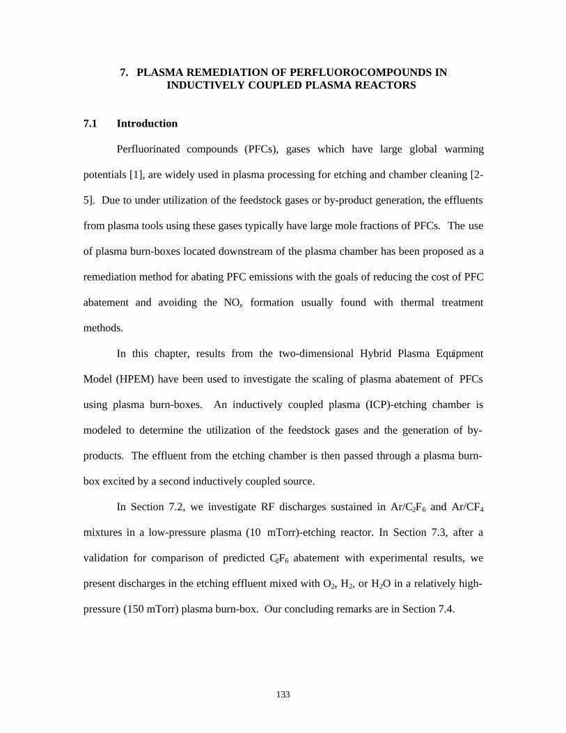
133
7. PLASMA REMEDIATION OF PERFLUOROCOMPOUNDS ININDUCTIVELY COUPLED PLASMA REACTORS
7.1 Introduction
Perfluorinated compounds (PFCs), gases which have large global warming
potentials [1], are widely used in plasma processing for etching and chamber cleaning [2-
5]. Due to under utilization of the feedstock gases or by-product generation, the effluents
from plasma tools using these gases typically have large mole fractions of PFCs. The use
of plasma burn-boxes located downstream of the plasma chamber has been proposed as a
remediation method for abating PFC emissions with the goals of reducing the cost of PFC
abatement and avoiding the NOx formation usually found with thermal treatment
methods.
In this chapter, results from the two-dimensional Hybrid Plasma Equipment
Model (HPEM) have been used to investigate the scaling of plasma abatement of PFCs
using plasma burn-boxes. An inductively coupled plasma (ICP)-etching chamber is
modeled to determine the utilization of the feedstock gases and the generation of by-
products. The effluent from the etching chamber is then passed through a plasma burn-
box excited by a second inductively coupled source.
In Section 7.2, we investigate RF discharges sustained in Ar/C2F6 and Ar/CF4
mixtures in a low-pressure plasma (10 mTorr)-etching reactor. In Section 7.3, after a
validation for comparison of predicted C2F6 abatement with experimental results, we
present discharges in the etching effluent mixed with O2, H2, or H2O in a relatively high-
pressure (150 mTorr) plasma burn-box. Our concluding remarks are in Section 7.4.
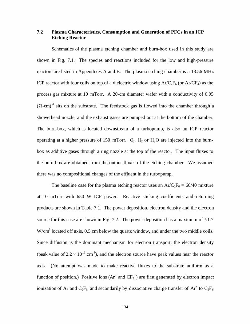
134
7.2 Plasma Characteristics, Consumption and Generation of PFCs in an ICPEtching Reactor
Schematics of the plasma etching chamber and burn-box used in this study are
shown in Fig. 7.1. The species and reactions included for the low and high-pressure
reactors are listed in Appendixes A and B. The plasma etching chamber is a 13.56 MHz
ICP reactor with four coils on top of a dielectric window using Ar/C2F6 (or Ar/CF4) as the
process gas mixture at 10 mTorr. A 20-cm diameter wafer with a conductivity of 0.05
(Ω-cm) -1 sits on the substrate. The feedstock gas is flowed into the chamber through a
showerhead nozzle, and the exhaust gases are pumped out at the bottom of the chamber.
The burn-box, which is located downstream of a turbopump, is also an ICP reactor
operating at a higher pressure of 150 mTorr. O2, H2 or H2O are injected into the burn-
box as additive gases through a ring nozzle at the top of the reactor. The input fluxes to
the burn-box are obtained from the output fluxes of the etching chamber. We assumed
there was no compositional changes of the effluent in the turbopump.
The baseline case for the plasma etching reactor uses an Ar/C2F6 = 60/40 mixture
at 10 mTorr with 650 W ICP power. Reactive sticking coefficients and returning
products are shown in Table 7.1. The power deposition, electron density and the electron
source for this case are shown in Fig. 7.2. The power deposition has a maximum of ≈1.7
W/cm3 located off axis, 0.5 cm below the quartz window, and under the two middle coils.
Since diffusion is the dominant mechanism for electron transport, the electron density
(peak value of 2.2 × 1011 cm-3), and the electron source have peak values near the reactor
axis. (No attempt was made to make reactive fluxes to the substrate uniform as a
function of position.) Positive ions (Ar+ and CF3+) are first generated by electron impact
ionization of Ar and C2F6, and secondarily by dissociative charge transfer of Ar+ to C2F6
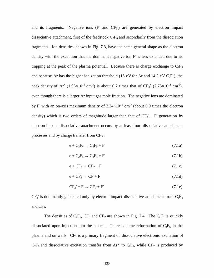
135
and its fragments. Negative ions (F- and CF3-) are generated by electron impact
dissociative attachment, first of the feedstock C2F6 and secondarily from the dissociation
fragments. Ion densities, shown in Fig. 7.3, have the same general shape as the electron
density with the exception that the dominant negative ion F- is less extended due to its
trapping at the peak of the plasma potential. Because there is charge exchange to C2F6
and because Ar has the higher ionization threshold (16 eV for Ar and 14.2 eV C2F6), the
peak density of Ar+ (1.96×1011 cm-3) is about 0.7 times that of CF3+ (2.75×1011 cm-3),
even though there is a larger Ar input gas mole fraction. The negative ions are dominated
by F- with an on-axis maximum density of 2.24×1011 cm-3 (about 0.9 times the electron
density) which is two orders of magnitude larger than that of CF3-. F- generation by
electron impact dissociative attachment occurs by at least four dissociative attachment
processes and by charge transfer from CF3-,
e + C2F6 → C2F5 + F- (7.1a)
e + C2F5 → C2F4 + F- (7.1b)
e + CF3 → CF2 + F- (7.1c)
e + CF2 → CF + F- (7.1d)
CF3- + F → CF3 + F- (7.1e)
CF3- is dominantly generated only by electron impact dissociative attachment from C2F6
and CF4.
The densities of C2F6, CF3 and CF2 are shown in Fig. 7.4. The C2F6 is quickly
dissociated upon injection into the plasma. There is some reformation of C2F6 in the
plasma and on walls. CF3 is a primary fragment of dissociative electronic excitation of
C2F6 and dissociative excitation transfer from Ar* to C2F6, while CF2 is produced by
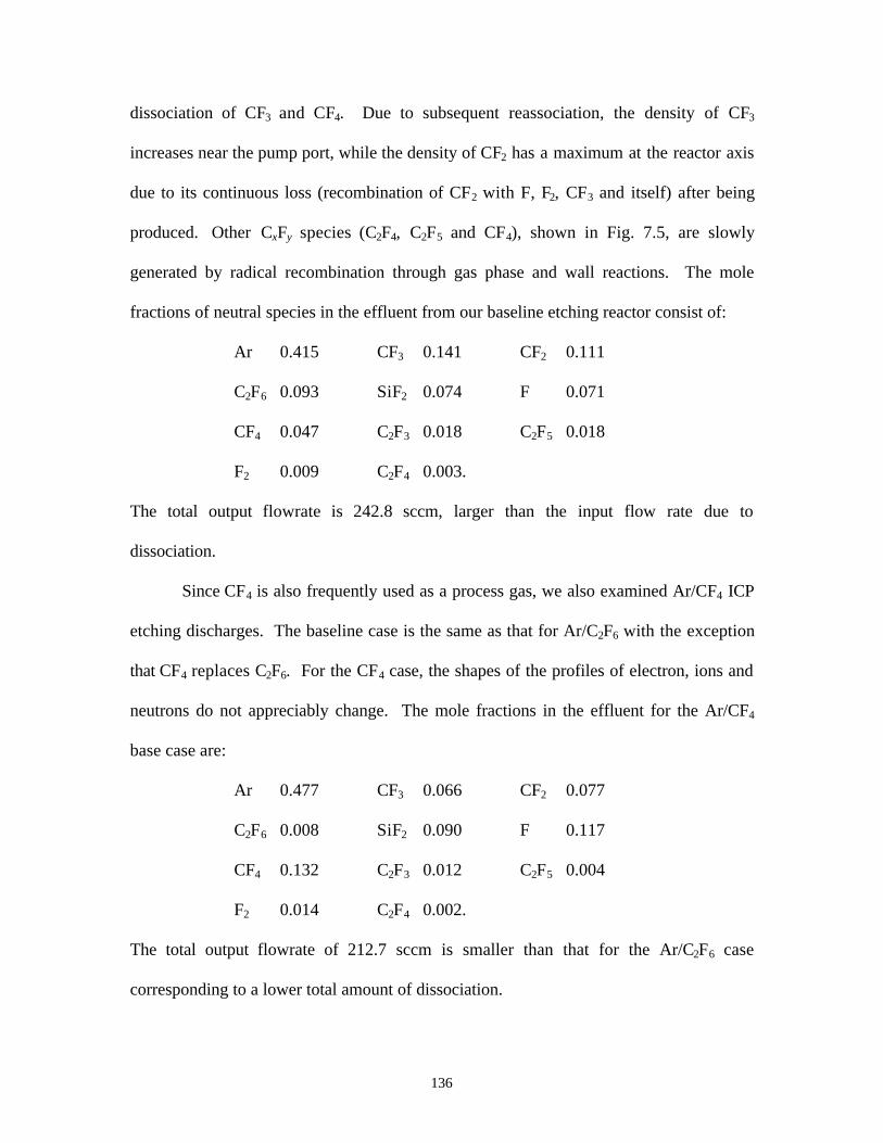
136
dissociation of CF3 and CF4. Due to subsequent reassociation, the density of CF3
increases near the pump port, while the density of CF2 has a maximum at the reactor axis
due to its continuous loss (recombination of CF2 with F, F2, CF3 and itself) after being
produced. Other CxFy species (C2F4, C2F5 and CF4), shown in Fig. 7.5, are slowly
generated by radical recombination through gas phase and wall reactions. The mole
fractions of neutral species in the effluent from our baseline etching reactor consist of:
Ar 0.415 CF3 0.141 CF2 0.111
C2F6 0.093 SiF2 0.074 F 0.071
CF4 0.047 C2F3 0.018 C2F5 0.018
F2 0.009 C2F4 0.003.
The total output flowrate is 242.8 sccm, larger than the input flow rate due to
dissociation.
Since CF4 is also frequently used as a process gas, we also examined Ar/CF4 ICP
etching discharges. The baseline case is the same as that for Ar/C2F6 with the exception
that CF4 replaces C2F6. For the CF4 case, the shapes of the profiles of electron, ions and
neutrons do not appreciably change. The mole fractions in the effluent for the Ar/CF4
base case are:
Ar 0.477 CF3 0.066 CF2 0.077
C2F6 0.008 SiF2 0.090 F 0.117
CF4 0.132 C2F3 0.012 C2F5 0.004
F2 0.014 C2F4 0.002.
The total output flowrate of 212.7 sccm is smaller than that for the Ar/C2F6 case
corresponding to a lower total amount of dissociation.
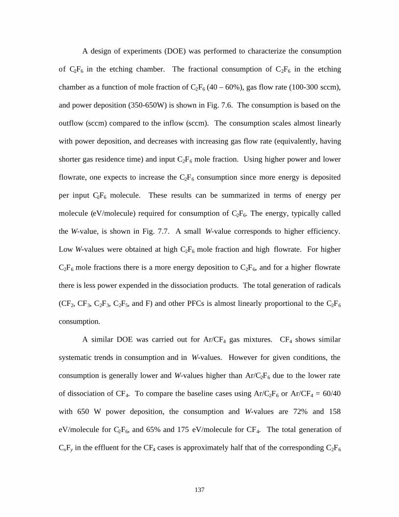
137
A design of experiments (DOE) was performed to characterize the consumption
of C2F6 in the etching chamber. The fractional consumption of C2F6 in the etching
chamber as a function of mole fraction of C2F6 (40 – 60%), gas flow rate (100-300 sccm),
and power deposition (350-650W) is shown in Fig. 7.6. The consumption is based on the
outflow (sccm) compared to the inflow (sccm). The consumption scales almost linearly
with power deposition, and decreases with increasing gas flow rate (equivalently, having
shorter gas residence time) and input C2F6 mole fraction. Using higher power and lower
flowrate, one expects to increase the C2F6 consumption since more energy is deposited
per input C2F6 molecule. These results can be summarized in terms of energy per
molecule (eV/molecule) required for consumption of C2F6. The energy, typically called
the W-value, is shown in Fig. 7.7. A small W-value corresponds to higher efficiency.
Low W-values were obtained at high C2F6 mole fraction and high flowrate. For higher
C2F6 mole fractions there is a more energy deposition to C2F6, and for a higher flowrate
there is less power expended in the dissociation products. The total generation of radicals
(CF2, CF3, C2F3, C2F5, and F) and other PFCs is almost linearly proportional to the C2F6
consumption.
A similar DOE was carried out for Ar/CF4 gas mixtures. CF4 shows similar
systematic trends in consumption and in W-values. However for given conditions, the
consumption is generally lower and W-values higher than Ar/C2F6 due to the lower rate
of dissociation of CF4. To compare the baseline cases using Ar/C2F6 or Ar/CF4 = 60/40
with 650 W power deposition, the consumption and W-values are 72% and 158
eV/molecule for C2F6, and 65% and 175 eV/molecule for CF4. The total generation of
CxFy in the effluent for the CF4 cases is approximately half that of the corresponding C2F6
138
cases. The output amounts of CF2 and CF3 for the C2F6 case are larger by factors of 2.44
and 1.65, respectively, compared to the CF4 case, largely a consequence of the branching
ratios for fragmentation of the feedstocks which favor CFx production from C2F6. There
are, however, slightly more F radicals in the effluent for Ar/CF4 mixtures.
7.3 Plasma Abatement of PFCs in a Burn-Box
In order to abate the PFCs emitted by the etching chamber, the effluent is passed
through the plasma burn-box. The effluents for Ar/C2F6 discharges consist mainly of Ar,
undissociated C2F6, CFx radicals, newly generated PFCs (CF4, C2F4, and C2F5), fluorine
(F and F2), and the etch product (SiF2). In this section we first present a comparison
between our computed results and those measured experimentally for abatement of C2F6
for validation purposes, and then discuss the remediation of simulated effluent from the
plasma etching chamber using O2, H2, or H2O as additives.
7.3.1 Validation
The plasma remediation model was validated by comparing our results to
experiments by Sawin and Vitale [6] for abatement of C2F6 in an ICP reactor. Their
reactor is a 10-cm diameter stainless steel tube with an internal coil. The feedstock gas
was C2F6/O2 = 50/50. They found that C2F6 is decomposed in the plasma reactor, but CF4
is generated as a product, which coincides with the observations of Hartz et al. [7].
The formation of CF4 largely depends on the availability of F atoms to recombine
with CF3. Through our parameterizations, we found that the branching ratio for e + C2F6
→ C2F5 + F- or CF3 + CF3- significantly affects the net destruction of C2F6 and the
139
formation of CF4 for Sawin and Vitale’s conditions. For example, the mole fractions of
C2F6 remaining and CF4 formation in the exhaust of the burn-box are shown in Fig. 7.8(a)
as a function of the branching ratio of e + C2F6 → CF3 + CF3-. The total flowrate is 400
sccm, the pressure is 500 mTorr, and the power deposition is 500 W. An increase in this
branching (and decrease in branching for C2F5 + F-) produces more CF3, which can
recombine more rapidly with F to form CF4 and with another CF3 radicals to reform C2F6.
Any C2F5 generated can rapidly react with F to generate additional CF3. A branching
ratio of 58% best matches experimental data. Using this branching, comparisons between
experiments and simulations as a function of power deposition are shown in Fig. 7.8(b).
Over the range of power investigated, the model agrees well with the experiments. The
C2F6 destruction increases with increasing power while the CF4 production increases. At
the highest power (1000 W) there is 40% C2F6 decomposition and 25% CF4 generation.
At 500 mTorr, the plasma is generated dominantly near the coils due to the finite
electromagnetic skin depth and rapid electron thermalization. For example, the electron
density and the rate of electron impact dissociation of C2F6 are shown in Fig. 7.9, along
with the advective gas velocity field, for the 500 W case. The maximum electron density
(5.3 × 1011 cm-3) is near the middle coil and decreases by a factor of 30 at the center of
the burn-box. The dissociation rate of C2F6 is correspondingly smaller in the center
where the advective gas velocity is highest. This pass through of gases in the center of
reactor contributes to the lower level of C2F6 degradation under the experimental
condition [6].
As will be discussed later, CF4 generation is via radical recombination between F
and CF3. At 500 mTorr, the rate constant of CF3 + F → CF4 is given by [8]
140
−
×=
−
−
gas
gas
T
Tk
2210exp
2981053
737
82
.
. cm3/s (7.2)
where Tgas is the gas temperature. At 500 W, the mean gas temperature in the reactor is
≈400 K, at which k9 = 1.1 × 10⁻¹¹ cm3/s. As a result CF4 production is favored. Higher
mean gas temperatures result in lower rates of CF4 production, as will be discussed
below.
W-values for C2F6 and for all CxFy as a function of power for the experimental
conditions are shown in Fig. 7.10. To quantify the destruction efficiency of all CxFy
species, we define its W-value as the input energy divided by the sum of CxFy destruction
weighted by the number of F atoms and normalized by 6 (the number of F atoms in
C2F6),
( )∑ ∑ ⋅−⋅
=
i ioutputyxiinputyxi
yx yFyF
PW
]/)([]/)([ 6FC6FCFC (7.3)
where P is the power deposition, Fi is the flow rate (input or output) of ith CxFy. The W-
value would equal that for C2F6 if it was completely oxidized with there being no CxFy
fragments. The weighting of the W-value with the number of F atoms in the molecule is
a qualitative judgment that larger dissociation products are “less good.” W(CxFy)-value is
5-10 times larger than W(C2F6)-value since more energy is required to abate the products
of the dissociation of C2F6 than to simply destroy C2F6. Both W-values increase with
increasing power, indicating lower efficiency. Although higher power deposition
produces higher densities of radicals, the higher radical densities result in more rapid
radical-radical recombination reactions. As the power deposition increases and more
141
dissociation is produced, the incremental dissociation is less efficient because more
power goes into the dissociation products.
7.3.2 O2 as an additive for PFC abatement
We first consider O2 as an additive gas for PFC abatement of effluent from the
etching chamber in the plasma burn-box. The desired reaction pathway is to oxidize CxFy
to CO2. Electron impact of O2 generates O, O(1D) and O+, which in turn react with the
PFCs and CFx radicals mainly as follows:
O [or O(1D)] + CF3 → COF2 + F k4a = 3.1×10⁻¹¹ cm3 s-1 (7.4a)
O [or O(1D)] + CF2 → COF + F k4b = 1.4×10⁻¹¹ cm3 s-1 (7.4b)
O [or O(1D)] + CF → CO + F k4c = 2.4×10⁻¹¹ cm3 s-1 (7.4c)
O+ + C2F6 → C2F5+ + FO k4d = 3.0×10⁻¹¹ cm3 s-1 (7.4d)
→ CF3+ + CF3 + O k4e = 1.5×10⁻⁹ cm3 s-1 (7.4e)
O+ + CF4 → CF3+ + FO k4f = 1.4×10⁻⁹ cm3 s-1 (7.4f)
where rate coefficients are shown for Tg = 500 K. The dominant reaction products of O
atoms with CFx are COF, COF2, and CO. It is important to note that at low gas
temperatures O and O(1D) do not directly react with CF4 or C2F6, and O2 is generally
unreactive with CxFy fragments. Remediation dominantly occurs by radical-radical
reactions. The desired end product CO2 can be formed via further reactions of COF with
O or O(1D), and COF2 with O(1D).
142
O [or O(1D)] + COF → CO2 + F k5a = 9.3×10⁻¹¹ cm3 s-1 (7.5a)
O(1D) + COF2 → CO2 + F2 k5b = 5.3×10⁻¹¹ cm3 s-1 (7.5b)
Although PFC dissociation primarily takes place through electron impact, there are
several other pathways (e.g. dissociative charge transfer with O+, Ar+, F+, and F2+) for
dissociaiton. For example, approximately 62% of CF3 production is by direct electron
impact of C2F6 and 10% results from charge transfer reactions.
In our baseline case, the effluent comes into the burn-box through the top of the
reactor while O2 is injected through a ring nozzle pointing radially inward. The plasma
burn-box is cylindrical with an inner radius of 2.5 cm and a length of 26.5 cm. Two coils
are placed near the middle of the tube with a power deposition of 500 W. The effluent
from the plasma-etching reactor operating at Ar/C2F6 = 40/60, 200 sccm flowrate and 350
W power is used as input. This case was selected because its effluent contains a
relatively high mole fraction of C2F6 (0.289) with a variety of other CxFy species (0.173
CF3, 0.057 CF4, 0.055 CF2, 0.011 C2F4, and 0.02 C2F5). In addition, 150 sccm O2 is
injected from the nozzle on the side wall. The power deposition, electron density,
electron temperature, and plasma potential for this case are shown in Fig. 7.11. The peak
electron density is ≈1.2 × 1012 cm-3 with an off-axis maximum located 7.3 mm from the
side wall. The inductively coupled power deposition has a maximum of 15 W/cm3 and is
located approximately 3.3 mm inside the quartz tube. These peak values are larger than
the plasma etching chamber due to the higher power density (W/cm3) and the shorter
electron energy relaxation length at the higher pressure. The distance of the peak power
deposition from the wall is smaller than that in the plasma etching reactor due to the
143
shorter skin depth resulting from a higher electron density. The electron temperature,
peak value 3.1 eV, varies moderately near the coils in the radial direction and extends as
a "hot zone" about 5 cm above and below the coils.
As the gas passes through the volume rear the coils, the O2 density rapidly
decreases due to electron impact dissociation and ionization while the O density
increases, as shown in Fig. 7.12. For our baseline case, CF2 CF3, C2F3, C2F4, and C2F5
are nearly totally eliminated (~100%), and C2F6 is decreased by 53% in passing through
the burn-box. As shown in Figs. 7.12 and 7.13, their concentrations significantly
decrease as the gas flow passes through the region near the coils where the oxygen
radicals and electron densities are large. (O(1D) and O+ have high densities only in
plasma region since they react with other species or quench quickly after being
generated.) The concentrations of major oxidation products (CO, CO2, COF2) increase
downstream of the coil region as does CF4, as shown in Fig. 7.14. These oxidation
products can be remediated by conventional means. For example, COF2 is easily
removed by processing the gas stream through a water bubbler or water spray. This
method is also effective at removing the other major byproducts, such as F and F2. CO
can be converted to CO2 using a platinum catalyst. However CF4 is an undesirable by-
product since it is also a PFC with high global warming potential. A summary of the
abatement efficiencies and end-products for the base case appears in Table 7.2.
Note that a significant amount of CF4 is produced above the inlet value due to
back diffusion of F atoms produced lower in the reactor, which recombine with CF3. The
total amount of CF4 in the gas stream actually increases by a factor of 2.4 for the base
case. CF4 is primarily generated by recombination,
144
CF3 + F →M
CF4. (7.6)
The rate coefficient for this process is strongly dependent on gas temperature and
pressure. At 150 mTorr the rate coefficient is [8]
−
×=
−
−
g
g
T
Tk
41876exp
3001094
847
97
..
.
cm-3 s-1. (7.7)
The rates coefficient decreases by a factor of 4.5 by increasing the temperature from 300
K (k = 9.42 × 10⁻¹² cm3s-1) to 500 K (k = 2.09 × 10⁻¹² cm3s-1) and a factor of 158 with a
temperature increase to 1000 K (k = 5.97 × 10⁻¹⁴ cm3s-1). Therefore, generating CF4
could be reduced if the gas temperature is increased. For the base case, the wall
temperature is fixed at 400 K, resulting in a mean gas temperature in the burn-box of
≈500 K, at which the rate coefficient for CF4 formation is still large. By increasing the
wall temperature, the bulk gas temperature also increases, and the CF4 in the exhaust
decreases. This trend is shown in Fig. 7.15. The remaining C2F6 also decreases as the
wall and gas temperatures increase (and gas densities decrease) due to more favorable
overlap of the region of high-power deposition with the flow field of the C2F6. The
electron density shifts toward the center of the reactor due to the lower gas density.
The abatement of C2F6 and the generation of CF4 are shown in Fig. 7.16 as a
function of power and injected O2 for the output effluent from the plasma etching reactor
for the base case. [These results were obtained by performing a design-of-experiments
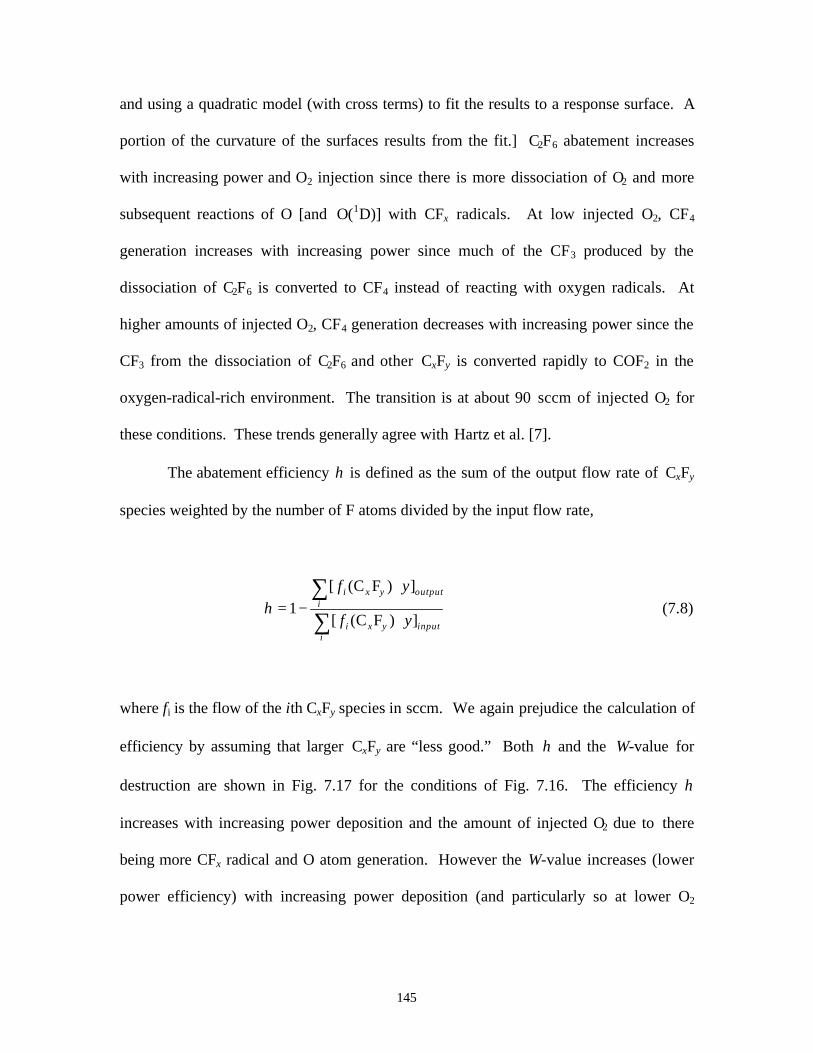
145
and using a quadratic model (with cross terms) to fit the results to a response surface. A
portion of the curvature of the surfaces results from the fit.] C2F6 abatement increases
with increasing power and O2 injection since there is more dissociation of O2 and more
subsequent reactions of O [and O(1D)] with CFx radicals. At low injected O2, CF4
generation increases with increasing power since much of the CF3 produced by the
dissociation of C2F6 is converted to CF4 instead of reacting with oxygen radicals. At
higher amounts of injected O2, CF4 generation decreases with increasing power since the
CF3 from the dissociation of C2F6 and other CxFy is converted rapidly to COF2 in the
oxygen-radical-rich environment. The transition is at about 90 sccm of injected O2 for
these conditions. These trends generally agree with Hartz et al. [7].
The abatement efficiency η is defined as the sum of the output flow rate of CxFy
species weighted by the number of F atoms divided by the input flow rate,
∑∑
⋅
⋅−=
iinputyxi
ioutputyxi
yf
yf
])FC([
])FC([
1η (7.8)
where fi is the flow of the ith CxFy species in sccm. We again prejudice the calculation of
efficiency by assuming that larger CxFy are “less good.” Both η and the W-value for
destruction are shown in Fig. 7.17 for the conditions of Fig. 7.16. The efficiency η
increases with increasing power deposition and the amount of injected O2 due to there
being more CFx radical and O atom generation. However the W-value increases (lower
power efficiency) with increasing power deposition (and particularly so at lower O2
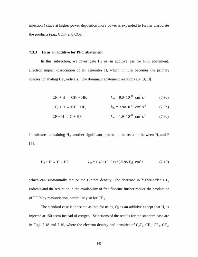
146
injection ) since at higher power deposition more power is expended to further dissociate
the products (e.g., COF2 and CO2).
7.3.3 H2 as an additive for PFC abatement
In this subsection, we investigate H2 as an additive gas for PFC abatement.
Electron impact dissociation of H2 generates H, which in turn becomes the primary
species for abating CFx radicals. The dominant abatement reactions are [9,10]
CF3 + H → CF2 + HF, k9a = 9.0×10⁻¹¹ cm3 s-1 (7.9a)
CF2 + H → CF + HF, k9b = 3.9×10⁻¹¹ cm3 s-1 (7.9b)
CF + H → C + HF, k9c = 1.9×10⁻¹¹ cm3 s-1 (7.9c)
In mixtures containing H2, another significant process is the reaction between H2 and F
[9],
H2 + F → H + HF k10 = 1.43×10⁻¹⁰ exp(-528/Tg) cm3 s-1 (7.10)
which can substantially reduce the F atom density. The decrease in higher-order CFx
radicals and the reduction in the availability of free fluorine further reduce the production
of PFCs by reassociation, particularly so for CF4.
The standard case is the same as that for using O2 as an additive except that H2 is
injected at 150 sccm instead of oxygen. Selections of the results for the standard case are
in Figs. 7.18 and 7.19, where the electron density and densities of C2F6, CF4, CF3, CF2,
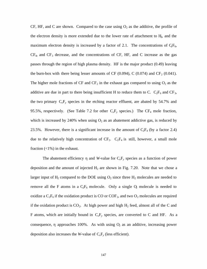
147
CF, HF, and C are shown. Compared to the case using O2 as the additive, the profile of
the electron density is more extended due to the lower rate of attachment to H2, and the
maximum electron density is increased by a factor of 2.1. The concentrations of C2F6,
CF4, and CF3 decrease, and the concentrations of CF, HF, and C increase as the gas
passes through the region of high plasma density. HF is the major product (0.49) leaving
the burn-box with there being lesser amounts of CF (0.094), C (0.074) and CF2 (0.041).
The higher mole fractions of CF and CF2 in the exhaust gas compared to using O2 as the
additive are due in part to there being insufficient H to reduce them to C. C2F6 and CF3,
the two primary CxFy species in the etching reactor effluent, are abated by 54.7% and
95.5%, respectively. (See Table 7.2 for other CxFy species.) The CF4 mole fraction,
which is increased by 240% when using O2 as an abatement addictive gas, is reduced by
23.5%. However, there is a significant increase in the amount of C2F4 (by a factor 2.4)
due to the relatively high concentration of CF2. C2F4 is still, however, a small mole
fraction (<1%) in the exhaust.
The abatement efficiency η and W-value for CxFy species as a function of power
deposition and the amount of injected H2 are shown in Fig. 7.20. Note that we chose a
larger input of H2 compared to the DOE using O2 since three H2 molecules are needed to
remove all the F atoms in a C2F6 molecule. Only a single O2 molecule is needed to
oxidize a C2F6 if the oxidation product is CO or COF2, and two O2 molecules are required
if the oxidation product is CO2. At high power and high H2 feed, almost all of the C and
F atoms, which are initially bound in CxFy species, are converted to C and HF. As a
consequence, η approaches 100%. As with using O2 as an additive, increasing power
deposition also increases the W-value of CxFy (less efficient).
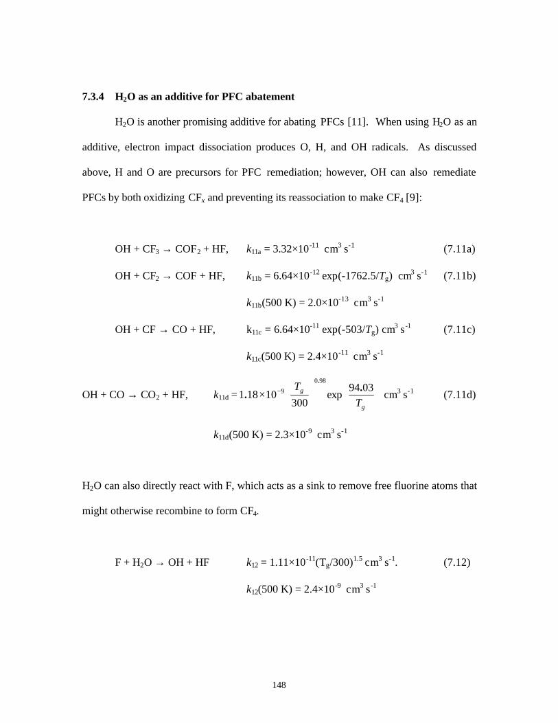
148
7.3.4 H2O as an additive for PFC abatement
H2O is another promising additive for abating PFCs [11]. When using H2O as an
additive, electron impact dissociation produces O, H, and OH radicals. As discussed
above, H and O are precursors for PFC remediation; however, OH can also remediate
PFCs by both oxidizing CFx and preventing its reassociation to make CF4 [9]:
OH + CF3 → COF2 + HF, k11a = 3.32×10⁻¹¹ cm3 s-1 (7.11a)
OH + CF2 → COF + HF, k11b = 6.64×10⁻¹² exp(-1762.5/Tg) cm3 s-1 (7.11b)
k11b(500 K) = 2.0×10⁻¹³ cm3 s-1
OH + CF → CO + HF, k11c = 6.64×10⁻¹¹ exp(-503/Tg) cm3 s-1 (7.11c)
k11c(500 K) = 2.4×10⁻¹¹ cm3 s-1
OH + CO → CO2 + HF, k11d
×= −
g
g
T
T 0394exp
30010181
980
9 ..
.
cm3 s-1 (7.11d)
k11d(500 K) = 2.3×10⁻⁹ cm3 s-1
H2O can also directly react with F, which acts as a sink to remove free fluorine atoms that
might otherwise recombine to form CF4.
F + H2O → OH + HF k12 = 1.11×10⁻¹¹(Tg/300)1.5 cm3 s-1. (7.12)
k12(500 K) = 2.4×10⁻⁹ cm3 s-1
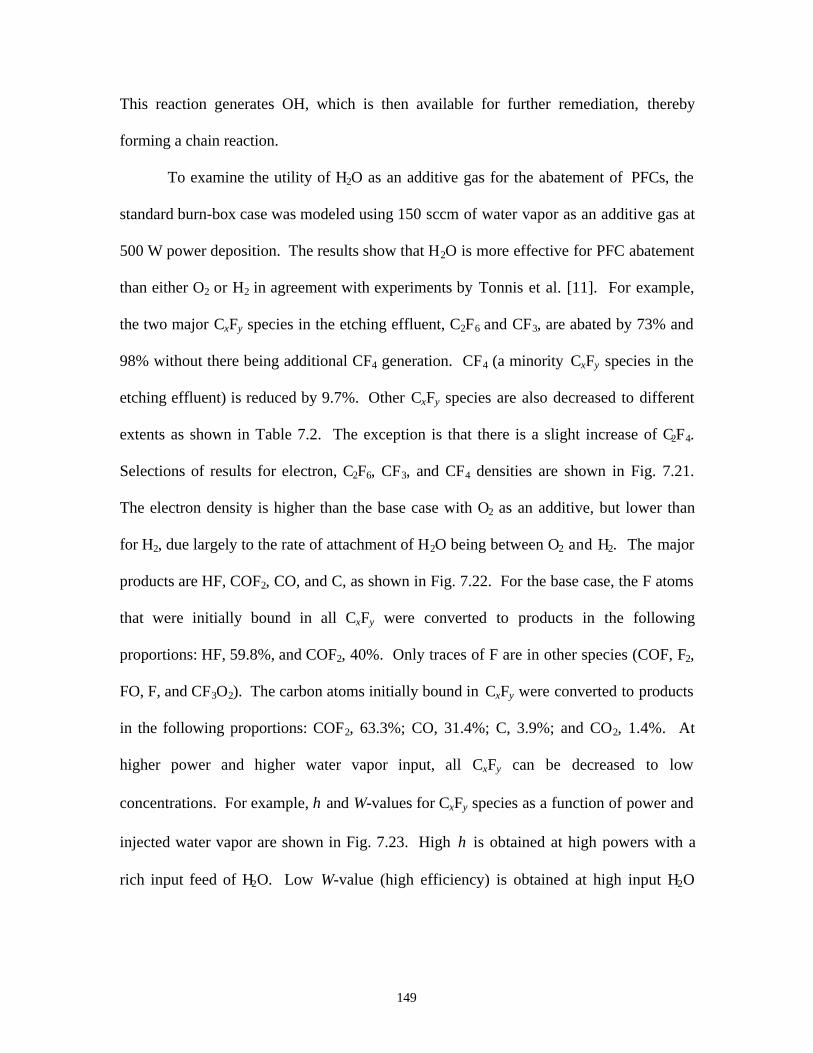
149
This reaction generates OH, which is then available for further remediation, thereby
forming a chain reaction.
To examine the utility of H2O as an additive gas for the abatement of PFCs, the
standard burn-box case was modeled using 150 sccm of water vapor as an additive gas at
500 W power deposition. The results show that H2O is more effective for PFC abatement
than either O2 or H2 in agreement with experiments by Tonnis et al. [11]. For example,
the two major CxFy species in the etching effluent, C2F6 and CF3, are abated by 73% and
98% without there being additional CF4 generation. CF4 (a minority CxFy species in the
etching effluent) is reduced by 9.7%. Other CxFy species are also decreased to different
extents as shown in Table 7.2. The exception is that there is a slight increase of C2F4.
Selections of results for electron, C2F6, CF3, and CF4 densities are shown in Fig. 7.21.
The electron density is higher than the base case with O2 as an additive, but lower than
for H2, due largely to the rate of attachment of H2O being between O2 and H2. The major
products are HF, COF2, CO, and C, as shown in Fig. 7.22. For the base case, the F atoms
that were initially bound in all CxFy were converted to products in the following
proportions: HF, 59.8%, and COF2, 40%. Only traces of F are in other species (COF, F2,
FO, F, and CF3O2). The carbon atoms initially bound in CxFy were converted to products
in the following proportions: COF2, 63.3%; CO, 31.4%; C, 3.9%; and CO2, 1.4%. At
higher power and higher water vapor input, all CxFy can be decreased to low
concentrations. For example, η and W-values for CxFy species as a function of power and
injected water vapor are shown in Fig. 7.23. High η is obtained at high powers with a
rich input feed of H2O. Low W-value (high efficiency) is obtained at high input H2O
150
flowrates with low power. These trends are similar to the cases using H2 additive except
for there being a higher efficiency and lower W-value.
7.4 Concluding Remarks
Results from a computational investigation of the consumption and generation of
PFCs in an ICP etching reactor for Ar/C2F6 and Ar/CF4 gas mixtures and the abatement
of the effluent in an ICP burn-box have been discussed. The model was validated by
comparison to experiments by Sawin and Vitale [6] using C2F6/O2 mixtures. C2F6 (or
CF4) consumption in the etching reactor is proportional to ICP power deposition, and
inversely proportional to C2F6 mole fraction and total gas flow rate. We found a ceiling
of 158 eV/molecule for consumption of C2F6 and 175 eV/molecule for CF4 for our
baseline cases, Ar/C2F6 (or Ar/CF4) = 60/40 at 500 W power deposition. The generation
of CxFy in the effluents for Ar/C2F6 gas mixtures is approximately twice that for Ar/CF4
gas mixture under the same conditions. There is slightly more generation of F and F2 for
the CF4 feedstock gas.
In general, CF4 generation occurs during abatement of C2F6 using O2 as an
additive, especially for high power with low O2 input due to low concentrations of O and
O(1D) atoms while there are large densities of F and CF3. At high gas temperatures, there
is a significant reduction of CF4 generation since the rate coefficient for recombination of
CF3 and F is strongly dependent on temperature. The major oxidation products are COF2,
CO and CO2. H2 can be used as an alternative to O2 for an abatement additive without
producing CF4 since hydrogen reacts rapidly with free fluorine which would otherwise
reassociate with CFx to form CF4. F and C atoms initially contained in CxFy were
151
converted to HF and C. Generation of C atoms could be problematic due to their
deposition on surfaces. It was also shown that H2O is a promising and efficient
abatement additive gas since it is a source of oxygen, hydrogen and hydroxyl radicals,
produced in beneficial mole fractions. The primary products of abatement using water
vapor are HF, CO, COF2 with small amounts of C and CO2.
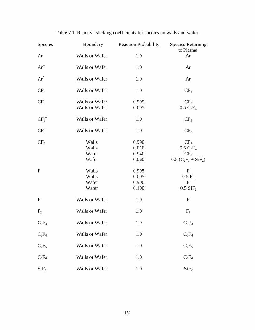
152
Table 7.1 Reactive sticking coefficients for species on walls and wafer.
Species Boundary Reaction Probability Species Returningto Plasma
Ar Walls or Wafer 1.0 Ar
Ar+ Walls or Wafer 1.0 Ar
Ar* Walls or Wafer 1.0 Ar
CF4 Walls or Wafer 1.0 CF4
CF3 Walls or Wafer 0.995 CF3
Walls or Wafer 0.005 0.5 C2F6
CF3+ Walls or Wafer 1.0 CF3
CF3- Walls or Wafer 1.0 CF3
CF2 Walls 0.990 CF2
Walls 0.010 0.5 C2F4
Wafer 0.940 CF2
Wafer 0.060 0.5 (C2F3 + SiF2)
F Walls 0.995 FWalls 0.005 0.5 F2
Wafer 0.900 FWafer 0.100 0.5 SiF2
F- Walls or Wafer 1.0 F
F2 Walls or Wafer 1.0 F2
C2F3 Walls or Wafer 1.0 C2F3
C2F4 Walls or Wafer 1.0 C2F4
C2F5 Walls or Wafer 1.0 C2F5
C2F6 Walls or Wafer 1.0 C2F6
SiF2 Walls or Wafer 1.0 SiF2
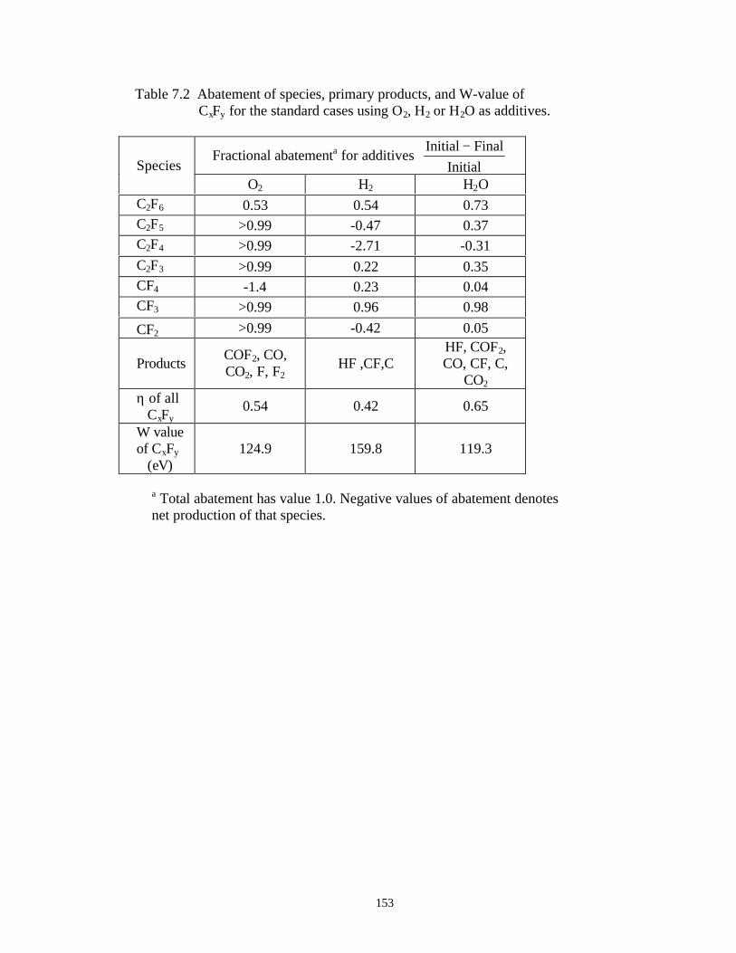
153
Table 7.2 Abatement of species, primary products, and W-value of CxFy for the standard cases using O2, H2 or H2O as additives.
Fractional abatementa for additives Initial
FinalInitial −Species
O2 H2 H2OC2F6 0.53 0.54 0.73C2F5 >0.99 -0.47 0.37C2F4 >0.99 -2.71 -0.31C2F3 >0.99 0.22 0.35CF4 -1.4 0.23 0.04CF3 >0.99 0.96 0.98
CF2 >0.99 -0.42 0.05
ProductsCOF2, CO,CO2, F, F2
HF ,CF,CHF, COF2,CO, CF, C,
CO2
η of all CxFy
0.54 0.42 0.65
W valueof CxFy
(eV)124.9 159.8 119.3
a Total abatement has value 1.0. Negative values of abatement denotes net production of that species.
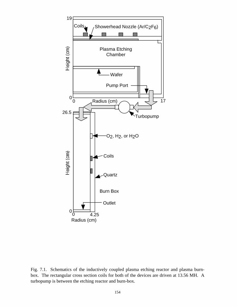
Plasma EtchingChamber
Wafer
Coils
O2, H2, or H2O
Burn Box
Coils
Showerhead Nozzle (Ar/C2F6)
Turbopump
0 170
19
0
26.5
0 4.25Radius (cm)
Radius (cm)
Pump Port
Quartz
Outlet
Fig. 7.1. Schematics of the inductively coupled plasma etching reactor and plasma burn-box. The rectangular cross section coils for both of the devices are driven at 13.56 MH. Aturbopump is between the etching reactor and burn-box.
154
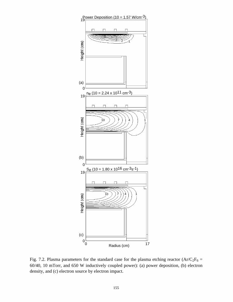
Power Deposition (10 = 1.57 W/cm-3)
123
0
19
(a)
10 7 4 1
ne (10 = 2.24 x 1011 cm-3)
0
19
(b)
Se (10 = 1.80 x 1016 cm-3s-1)
0
19
0 17Radius (cm)
10 7 4 1
(c)
Fig. 7.2. Plasma parameters for the standard case for the plasma etching reactor (Ar/C2F6 =60/40, 10 mTorr, and 650 W inductively coupled power): (a) power deposition, (b) electrondensity, and (c) electron source by electron impact.
155
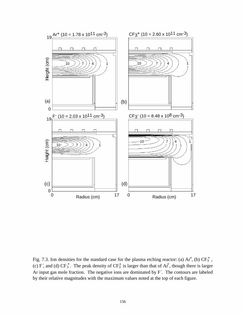
CF3+ (10 = 2.60 x 1011 cm-3)
10 7 4 1
(b)
0
19F- (10 = 2.03 x 1011 cm-3)
10 7 4 1
(c)
0 17Radius (cm)
CF3- (10 = 8.48 x 108 cm-3)
10 7 4 1
(d)
10 7 4 1
Ar+ (10 = 1.78 x 1011 cm-3)
(a)
0
19
0 17Radius (cm)
Fig. 7.3. Ion densities for the standard case for the plasma etching reactor: (a) Ar , (b) CF3 ,(c) F , and (d) CF3 . The peak density of CF3 is larger than that of Ar , though there is largerAr input gas mole fraction. The negative ions are dominated by F . The contours are labeledby their relative magnitudes with the maximum values noted at the top of each figure.
156
++
- + + +
-
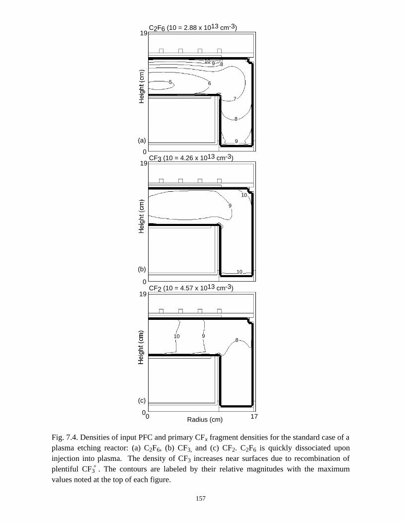
9
8
5 6
7
8910
C2F6 (10 = 2.88 x 1013 cm-3)
0
19
(a)
9
10
CF3 (10 = 4.26 x 1013 cm-3)
0
19
10(b)
10 98
0 17Radius (cm)
CF2 (10 = 4.57 x 1013 cm-3)
0
19
(c)
Fig. 7.4. Densities of input PFC and primary CFx fragment densities for the standard case of aplasma etching reactor: (a) C2F6, (b) CF3, and (c) CF2. C2F6 is quickly dissociated uponinjection into plasma. The density of CF3 increases near surfaces due to recombination ofplentiful CF3 . The contours are labeled by their relative magnitudes with the maximumvalues noted at the top of each figure.
157
+
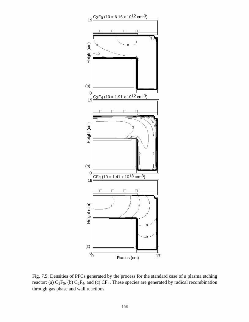
10
9 8
9
C2F5 (10 = 6.16 x 1012 cm-3)
0
19
(a)
3 4
5 5
6
C2F4 (10 = 1.91 x 1012 cm-3)
0
19
(b)
9
8
7
654
CF4 (10 = 1.41 x 1013 cm-3)
0
19
0 17Radius (cm)
(c)
Fig. 7.5. Densities of PFCs generated by the process for the standard case of a plasma etchingreactor: (a) C2F5, (b) C2F4, and (c) CF4. These species are generated by radical recombinationthrough gas phase and wall reactions.
158
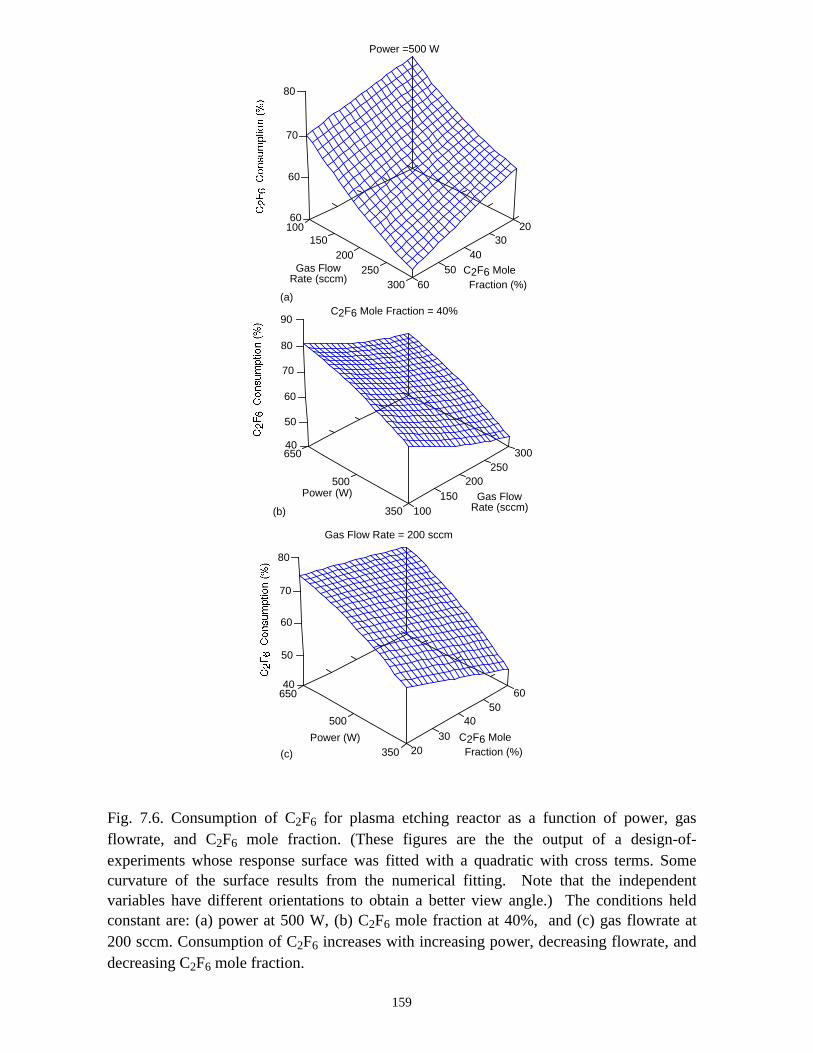
Power =500 W
2030
4050
60
Gas FlowRate (sccm)
100150
200250
300
60
70
60
C2F6 Mole Fraction (%)
80
(a)C2F6 Mole Fraction = 40%
Power (W) Gas FlowRate (sccm)
650
500
350
50
80
60
70
100150
200250
300
90
40
(b)
Gas Flow Rate = 200 sccm
C2F6 Mole Fraction (%)
Power (W)
650
500
350 2030
4050
60
50
60
70
40
80
(c)
Fig. 7.6. Consumption of C2F6 for plasma etching reactor as a function of power, gasflowrate, and C2F6 mole fraction. (These figures are the the output of a design-of-experiments whose response surface was fitted with a quadratic with cross terms. Somecurvature of the surface results from the numerical fitting. Note that the independentvariables have different orientations to obtain a better view angle.) The conditions heldconstant are: (a) power at 500 W, (b) C2F6 mole fraction at 40%, and (c) gas flowrate at200 sccm. Consumption of C2F6 increases with increasing power, decreasing flowrate, anddecreasing C2F6 mole fraction.
159
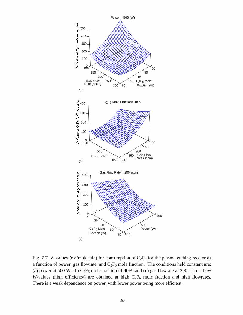
Power = 500 (W)
100
200
300
20
40
60
Gas FlowRate (sccm)
C2F6 Mole Fraction (%)
0
100
200
300
400
150
250
500
50
30
(a)
C2F6 Mole Fraction= 40%
300
100
200
300
0350
500
650
200
100
Power (W) Gas FlowRate (sccm)
250
150
400
(b)
Gas Flow Rate = 200 sccm
300
100
0350
500
65060
40
20
Power (W)
30
50
400
200
C2F6 MoleFraction (%)
(c)
Fig. 7.7. W-values (eV/molecule) for consumption of C2F6 for the plasma etching reactor asa function of power, gas flowrate, and C2F6 mole fraction. The conditions held constant are:(a) power at 500 W, (b) C2F6 mole fraction of 40%, and (c) gas flowrate at 200 sccm. LowW-values (high efficiency) are obtained at high C2F6 mole fraction and high flowrates.There is a weak dependence on power, with lower power being more efficient.
160
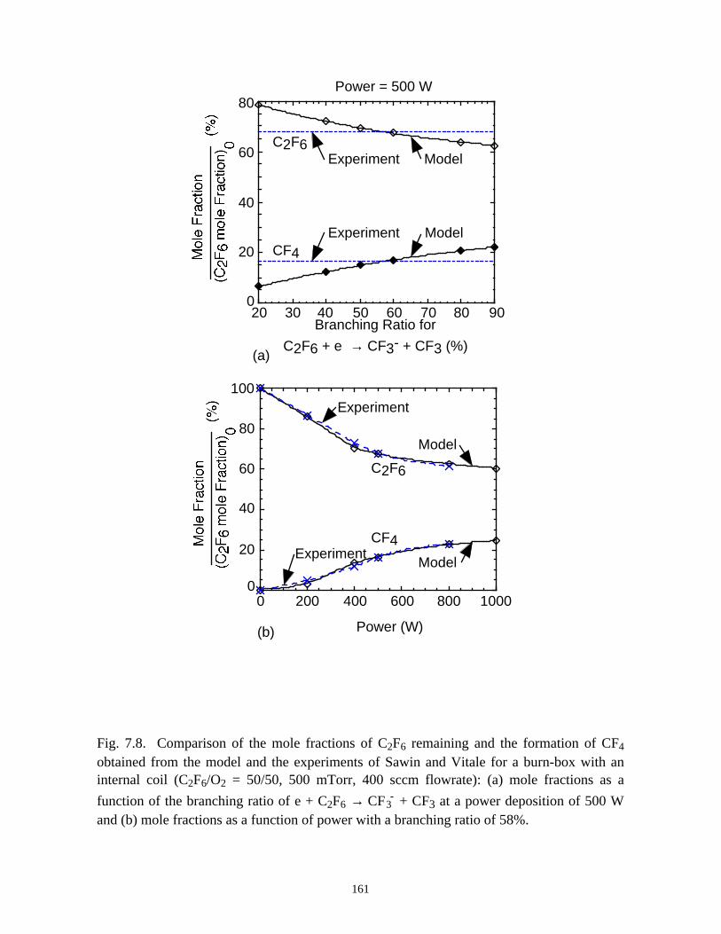
Experiment
Model
Model
C2F6
CF4
0
20
40
60
80
100
0 200 400 600 800 1000
Power (W)(b)
Power = 500 W
20 30 40 50 60 70 80 90Branching Ratio for
C2F6 + e → CF3- + CF3 (%)
0
20
60
80
C2F6
CF4Model
ModelExperiment
40
(a)
Experiment
Experiment
Fig. 7.8. Comparison of the mole fractions of C2F6 remaining and the formation of CF4
obtained from the model and the experiments of Sawin and Vitale for a burn-box with aninternal coil (C2F6/O2 = 50/50, 500 mTorr, 400 sccm flowrate): (a) mole fractions as a
function of the branching ratio of e + C2F6 → CF3 + CF3 at a power deposition of 500 Wand (b) mole fractions as a function of power with a branching ratio of 58%.
161
-
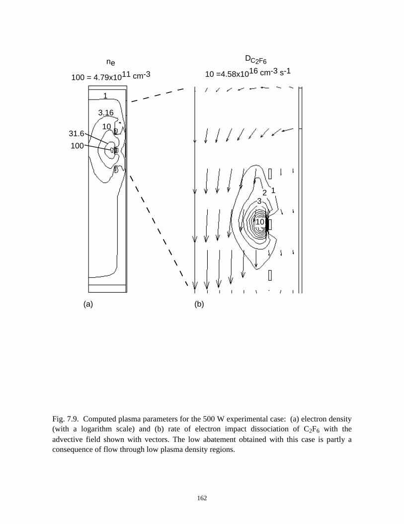
100
31.610
3.16
1
ne
100 = 4.79x1011 cm-3
D
10 =4.58x1016 cm-3 s-1C2F6
10
1
(a) (b)
23
Fig. 7.9. Computed plasma parameters for the 500 W experimental case: (a) electron density(with a logarithm scale) and (b) rate of electron impact dissociation of C2F6 with theadvective field shown with vectors. The low abatement obtained with this case is partly aconsequence of flow through low plasma density regions.
162
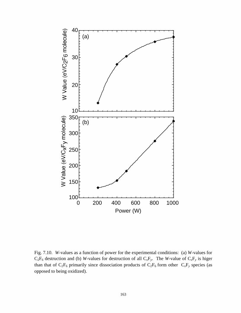
10
20
30
40
0 200 400 600 800 1000Power (W)
100
200
300
150
250
350
(a)
(b)
Fig. 7.10. W-values as a function of power for the experimental conditions: (a) W-values forC2F6 destruction and (b) W-values for destruction of all CxFy. The W-value of CxFy is higerthan that of C2F6 primarily since dissociation products of C2F6 form other CxFy species (asopposed to being oxidized).
163
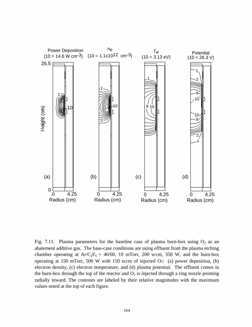
Te(10 = 3.13 eV)
1
10
0 4.25Radius (cm)
9
(c)
0 4.25Radius (cm)
Potential(10 = 26.3 V)
10
1
10
1
2
2
9
9
(d)
Power Deposition (10 = 14.6 W cm-3)
10
1
0
26.5
(a)
0 4.25Radius (cm)
10
ne(10 = 1.1x1012 cm-3)
2
1
(b)
0 4.25Radius (cm)
Fig. 7.11. Plasma parameters for the baseline case of plasma burn-box using O2 as anabatement additive gas. The base-case conditions are using effluent from the plasma etchingchamber operating at Ar/C2F6 = 40/60, 10 mTorr, 200 sccm, 350 W, and the burn-boxoperating at 150 mTorr, 500 W with 150 sccm of injected O2: (a) power deposition, (b)electron density, (c) electron temperature, and (d) plasma potential. The effluent comes inthe burn-box through the top of the reactor and O2 is injected through a ring nozzle pointingradially inward. The contours are labeled by their relative magnitudes with the maximumvalues noted at the top of each figure.
164
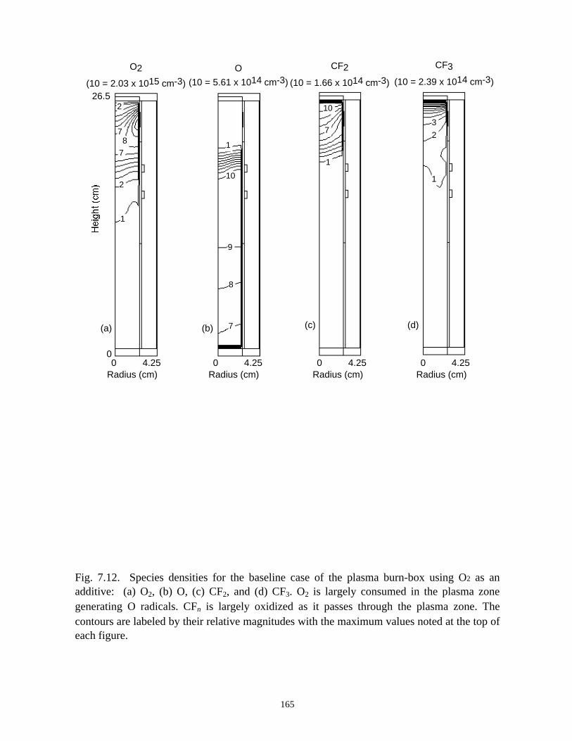
CF2
(10 = 1.66 x 1014 cm-3)
10
1
0 4.25Radius (cm)
7
(c)
CF3
(10 = 2.39 x 1014 cm-3)
1
2
3
0 4.25Radius (cm)
(d)
O2
(10 = 2.03 x 1015 cm-3)
0
26.5
8
2
7
7
2
1
(a)
0 4.25Radius (cm)
1
10
9
8
7
O
(10 = 5.61 x 1014 cm-3)
(b)
0 4.25Radius (cm)
Fig. 7.12. Species densities for the baseline case of the plasma burn-box using O2 as anadditive: (a) O2, (b) O, (c) CF2, and (d) CF3. O2 is largely consumed in the plasma zonegenerating O radicals. CFn is largely oxidized as it passes through the plasma zone. Thecontours are labeled by their relative magnitudes with the maximum values noted at the top ofeach figure.
165
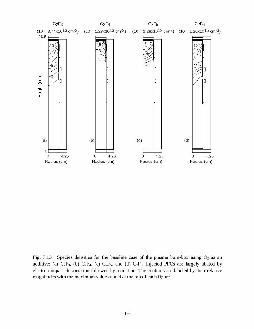
1
10
C2F3
(10 = 3.74x1013 cm-3)
0
26.5
2
5
7
(a)
1
C2F4
(10 = 1.28x1013 cm-3)
3
5
(b)
1
10
C2F5
(10 = 1.28x1013 cm-3)
0 4.25Radius (cm)
5
(c)
10
8 7
7
23
C2F6
(10 = 1.20x1015 cm-3)
0 4.25Radius (cm)
(d)
0 4.25Radius (cm)
0 4.25Radius (cm)
Fig. 7.13. Species densities for the baseline case of the plasma burn-box using O2 as anadditive: (a) C2F3, (b) C2F4, (c) C2F5, and (d) C2F6. Injected PFCs are largely abated byelectron impact dissociation followed by oxidation. The contours are labeled by their relativemagnitudes with the maximum values noted at the top of each figure.
166
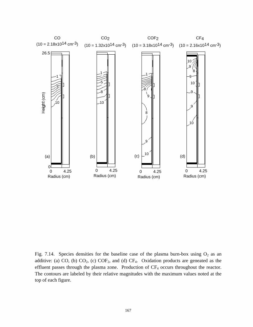
COF2
(10 = 3.18x1014 cm-3)
1
8
8
9
9
10
0 4.25Radius (cm)
(c)
CF4
(10 = 2.16x1014 cm-3)
109
9
9
8
9
10
10
0 4.25Radius (cm)
(d)
1
10
CO
(10 = 2.18x1014 cm-3)
0
26.5
5
(a)
0 4.25Radius (cm)
10
1
CO2
(10 = 1.32x1014 cm-3)
8
5
(b)
0 4.25Radius (cm)
Fig. 7.14. Species densities for the baseline case of the plasma burn-box using O2 as anadditive: (a) CO, (b) CO2, (c) COF2, and (d) CF4. Oxidation products are geneated as theeffluent passes through the plasma zone. Production of CF4 occurs throughout the reactor.The contours are labeled by their relative magnitudes with the maximum values noted at thetop of each figure.
167
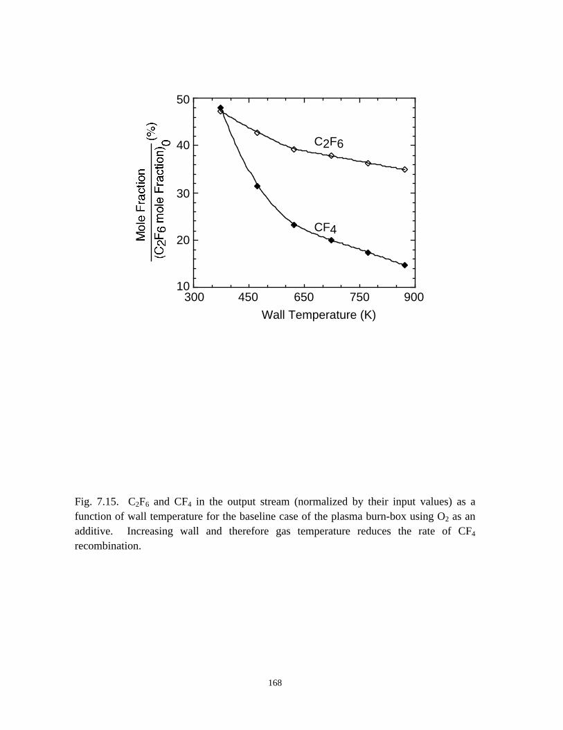
300 450 650 750 900
Wall Temperature (K)
10
20
30
40
50
CF4
C2F6
Fig. 7.15. C2F6 and CF4 in the output stream (normalized by their input values) as afunction of wall temperature for the baseline case of the plasma burn-box using O2 as anadditive. Increasing wall and therefore gas temperature reduces the rate of CF4
recombination.
168
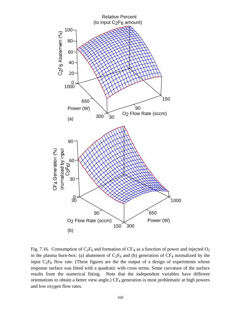
30
90
150
1000
650
300
20
40
60
80
100
Power (W)O2 Flow Rate (sccm)
Relative Percent(to input C2F6 amount)
30
90
150
1000
650
300Power (W)O2 Flow Rate (sccm)
30
60
90
0
0
(a)
(b)
Fig. 7.16. Consumption of C2F6 and formation of CF4 as a function of power and injected O2
in the plasma burn-box: (a) abatement of C2F6 and (b) generation of CF4 normalized by theinput C2F6 flow rate. (These figures are the the output of a design of experiments whoseresponse surface was fitted with a quadratic with cross terms. Some curvature of the surfaceresults from the numerical fitting. Note that the independent variables have differentorientations to obtain a better view angle.) CF4 generation is most problematic at high powersand low oxygen flow rates.
169
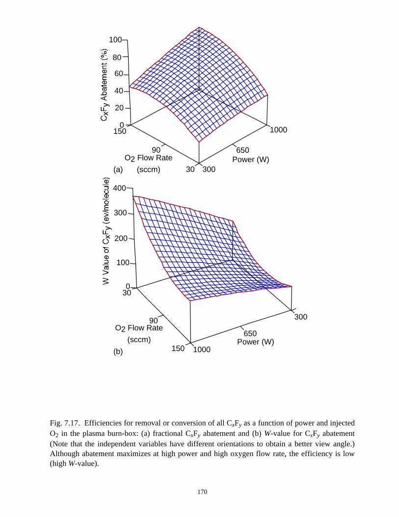
30
90
150 1000
650
300
40
60
80
100
Power (W)O2 Flow Rate
(sccm)
20
0
30
90
150 1000
650
300
300
200
400
Power (W)
O2 Flow Rate
(sccm)
100
0
(a)
(b)
Fig. 7.17. Efficiencies for removal or conversion of all CxFy as a function of power and injectedO2 in the plasma burn-box: (a) fractional CxFy abatement and (b) W-value for CxFy abatement(Note that the independent variables have different orientations to obtain a better view angle.)Although abatement maximizes at high power and high oxygen flow rate, the efficiency is low(high W-value).
170
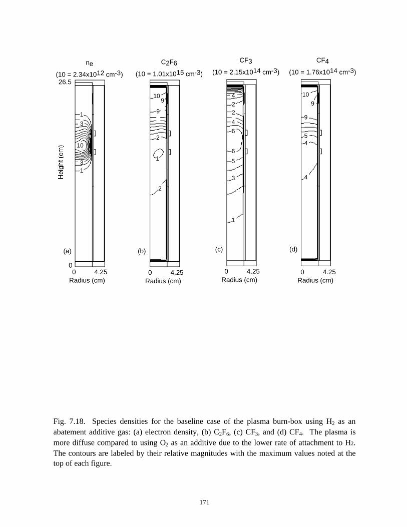
ne
(10 = 2.34x1012 cm-3)
10
1
1
C2F6
(10 = 1.01x1015 cm-3)
10
9
9
2
2
1
0
26.5
3
3
(a) (b)
CF3
(10 = 2.15x1014 cm-3)
22
1
6
6
5
3
CF4
(10 = 1.76x1014 cm-3)
10
9
9
54
4
0 4.25Radius (cm)
0 4.25Radius (cm)
4
4
(c) (d)
0 4.25Radius (cm)
0 4.25Radius (cm)
Fig. 7.18. Species densities for the baseline case of the plasma burn-box using H2 as anabatement additive gas: (a) electron density, (b) C2F6, (c) CF3, and (d) CF4. The plasma ismore diffuse compared to using O2 as an additive due to the lower rate of attachment to H2.The contours are labeled by their relative magnitudes with the maximum values noted at thetop of each figure.
171
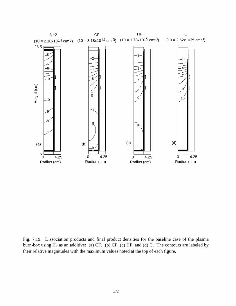
Fig. 7.19. Dissociation products and final product densities for the baseline case of the plasmaburn-box using H2 as an additive: (a) CF2, (b) CF, (c) HF, and (d) C. The contours are labeled bytheir relative magnitudes with the maximum values noted at the top of each figure.
172
CF2
(10 = 2.18x1014 cm-3)
CF
(10 = 3.18x1014 cm-3)
8
66
10
10
9
8
7
10
5
8
2
9
8
9
0
26.5
(a) (b)
HF
(10 = 1.73x1015 cm-3)
C
(10 = 2.62x1014 cm-3)
1
4
10
7
9
1
10
7
9
0 4.25Radius (cm)
0 4.25Radius (cm)
(c) (d)
4
0 4.25Radius (cm)
0 4.25Radius (cm)
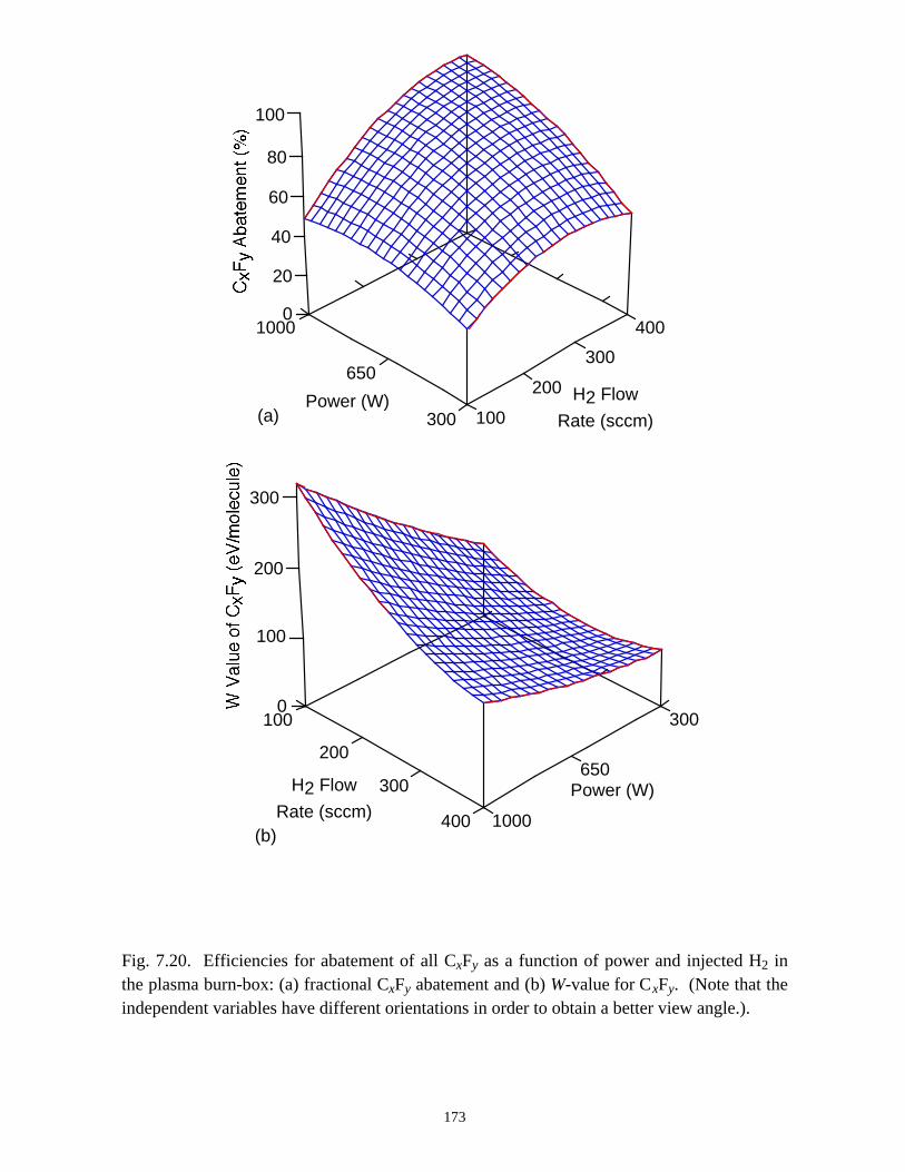
400
200
300H2 Flow
Rate (sccm)
100
1000
650
300
Power (W)
300
200
100
0
400
40
60
80
100
20
0
200
300
1000
650
300Power (W) H2 Flow
Rate (sccm)100(a)
(b)
Fig. 7.20. Efficiencies for abatement of all CxFy as a function of power and injected H2 inthe plasma burn-box: (a) fractional CxFy abatement and (b) W-value for CxFy. (Note that theindependent variables have different orientations in order to obtain a better view angle.).
173
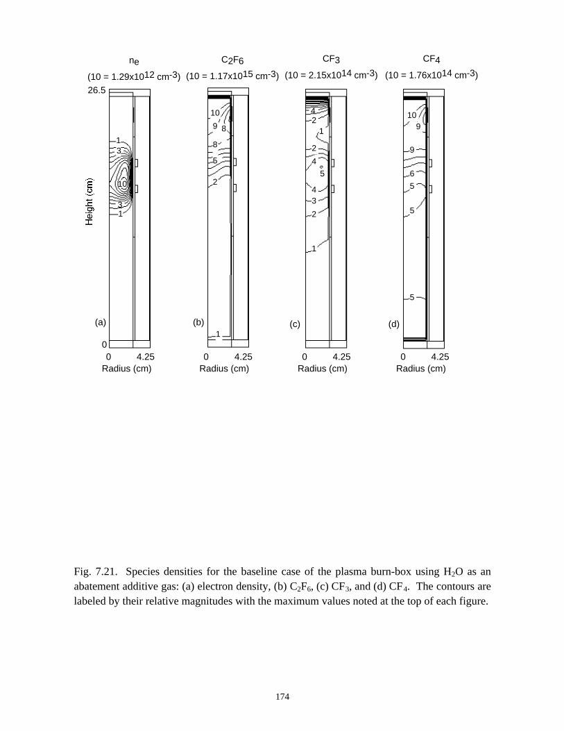
CF3
(10 = 2.15x1014 cm-3)
21
1
4
5
3
2
4
2
0 4.25Radius (cm)
4
(c)
CF4
(10 = 1.76x1014 cm-3)
109
9
5
6
5
5
0 4.25Radius (cm)
(d)
ne
(10 = 1.29x1012 cm-3)
1
1
0
26.5
10
3
3
(a)
0 4.25Radius (cm)
C2F6
(10 = 1.17x1015 cm-3)
10
89
2
1
8
5
(b)
0 4.25Radius (cm)
Fig. 7.21. Species densities for the baseline case of the plasma burn-box using H2O as anabatement additive gas: (a) electron density, (b) C2F6, (c) CF3, and (d) CF4. The contours arelabeled by their relative magnitudes with the maximum values noted at the top of each figure.
174
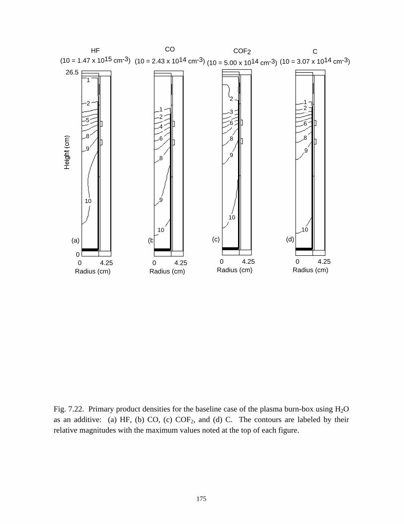
COF2
(10 = 5.00 x 1014 cm-3)
0 4.25Radius (cm)
10
8
9
2
3
6
(c)
0 4.25Radius (cm)
10
9
8
12
C
(10 = 3.07 x 1014 cm-3)
(d)
6
HF
(10 = 1.47 x 1015 cm-3)
10
5
9
2
1
8
0
26.5
(a) (b)
0 4.25Radius (cm)
CO
(10 = 2.43 x 1014 cm-3)
1
9
10
4
6
2
8
0 4.25Radius (cm)
Fig. 7.22. Primary product densities for the baseline case of the plasma burn-box using H2Oas an additive: (a) HF, (b) CO, (c) COF2, and (d) C. The contours are labeled by theirrelative magnitudes with the maximum values noted at the top of each figure.
175
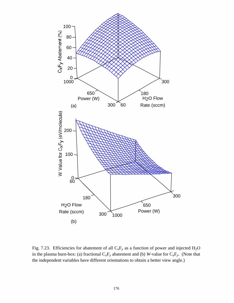
1000
650
300Power (W)
60
180
300
40
60
80
100
20
0
H2O Flow
Rate (sccm)
180
300
H2O Flow
Rate (sccm)
60
1000
650
300
Power (W)
200
100
0
(a)
(b)
Fig. 7.23. Efficiencies for abatement of all CxFy as a function of power and injected H2Oin the plasma burn-box: (a) fractional CxFy abatement and (b) W-value for CxFy. (Note thatthe independent variables have different orientations to obtain a better view angle.)
176
177
7.5 References
[1] J. V. Gompel and T. Walling, Semicond. Int., 95, (1997).
[2] K. Takahashi, M. Hori, and T. Goto, J. Vac. Sci. Technol. A14, 2004 (1996).
[3] M. A. Sobolewski, J. G. Langan, and B. S. Felker, J. Vac. Sci. Technol. B 16, 173
(1998).
[4] T. E. F. M. Standaert, M. Schaepkens, N. R. Rueger, P. G. M., Sebel, G. S.
Oehrlein, and J. M. Cook, J. Vac. Sci. Technol. A16, 239 (1998).
[5] B. E. E. Kastenmeier, P. J. Matsui, G. S. Oehrlein, and J. G. Langan, J. Vac. Sci.
Technol. A16, 2047 (1998).
[6] H. H. Sawin and S. A. Vitale, 51th Gaseous Electronics Conference, Maui,
Hawaii, Oct., 1998.
[7] C. L. Hartz, J, W. Bevaan, M. W. Jackson, and B. A. Wofford, Environ. Sci.
Technol. 32, 682 (1998).
[8] D. R. F. Burgess, Jr., National Institute of Standards and Technology (private
communication).
[9] D. R. F. Burgess, Jr., M. R. Zachariah, W. Tsang, and P. R. Westmoreland, Prog.
Energy Combust. Sci., 21, 453,1996.
[10] C. Tsai and D. L. McFadden, J. Phys. Chem. 93, 2471 (1989).
[11] E. J. Tonnis, V. Vartanian, L. Beu, T. Lii, R. Jewett, and D. Graves, Evaluation of
a Litmas “Blue” Point-of-Use (POU) Plasma Abatement Device for
Perfluorocompound (PFC) Destruction., SEMATECH Technology Transfer
98123605A-TR, 1998.
178
8. CONCLUDING REMARKS
One and two-dimensional plasma chemistry and hydrodynamics models have
been developed to study dielectric barrier discharge processing of high pressure gas
streams to be applied to micodischarge dynamics, toxic gas remediation, and UV and
VUV sources. The 2-D hybrid plasma equipment model has also been used to examine
low gas pressure plasma consumption and generation of PFCs in an ICP etching reactor
and abatement of PFCs in a plasma burn box. These models allow for a detailed study of
plasma induced chemical reactions and provide important insight into process trade-offs,
resulting in our ability to optimize the operation conditions.
The properties of the filamentary microdischarges found in dielectric barrier
discharges depend on the manner of charging of the dielectric. The charging of the
dielectric removes voltage from the gap thereby reducing E/N and producing a transition
from an avalanching discharge to a recombination or attachment dominated discharge.
Microdischarge dynamics have been investigated for gas mixtures with varying degrees
of electronegativity using the 1-D DBD model. In electropositive mixtures, the
expanding microdischarge maintains a fairly uniform electron density as a function of
radius, except for a small reduction in the core of the microdischarge due to electron-ion
recombination. In electronegative gas mixtures, the electron density has a maximum
value near the streamer edge due to dielectric charging and attachment at small radii at
lower E/N, especially for thermal attaching gas mixtures such as those containing CCl4.
We found that the expansion and ultimate stalling of the microdischarge is largely
determined by charging of dielectric at larger radii than the core of the microdischarge.
179
A 2-D DBD model has also been developed to investigate multiple-
microdischarge dynamics in dielectric barrier discharges. The closely spaced expanding
microdischarges retain their initial circular shapes until they collide and physically
contact. The avalanche stalls at the interface, but continues to expand on other sides.
The dynamics of adjacent microdischarges are similar to a single microdischarge, with
the exception that the electron density peaks at the interface by at most a few tens of
percent. The residual charge on the dielectric in DBDs from a preceding microdischarge
can significantly change the dynamics of microdischarges produced by the next voltage
pulse. The residual charge produces an additional voltage across the gap for the
subsequent microdischarge, thereby leading to more intense avalanche and providing a
mechanism for microdischarges to expand beyond their individual domains.
Remediation of carbon tetrachloride (CCl4) proceeds by a serial of chemical
reactions in DBDs. Though dissociative electron attachment is primarily responsible for
initial dissociation of CCl4, dissociative excitation and charge exchange from Ar*, Ar**,
Ar+, and O2+ to CCl4 also play significant roles. Decreasing the O2 mole fraction can
considerably increase the remediation efficiency of CCl4 due largely to enhancing the
dissociative excitation transfer. The optimum amount of O2 is 1−3 times that of Cl2 for
Ar/O2/CCl2 gas mixtures. The decrease in removal efficiency in the presence of small
amounts of water vapor results from the interception of Ar+ and O2+ by H2O. The
products of remediation are primarily COCl2 and ClO.
The excimer radiation from XeCl* at 308 nm, Xe2Cl* at 490 nm, and Xe2* at 172
nm was examined in DBDs in Xe/Cl2 gas mixtures. When the Cl2 mole fraction < 1%,
decreasing Cl2 decreases the XeCl* formation, but significantly improves the generation
180
of Xe2* and Xe2Cl* since the presence of Cl2 efficiently quenches Xe 2
* and Xe2Cl*. At
approximately 1% Cl2 there is an optimum efficiency for producing XeCl* due to a trade-
off between several reactions. When the Cl2 mole fraction exceeds the optimum, the
generation of XeCl* dominates, however its corresponding generation efficiency slowly
decreases with increasing Cl2. The strong attachment at high Cl2 concentration (≥ 5%)
leads to the electron density shell propagating to smaller radii after the pulse. Though
increasing dielectric capacitance increases all rates of excimer formation resulting due to
the higher energy deposition, the efficiencies of photon generation decreases. Higher
applied voltage improves both intensities and efficiencies of photon generation. At
higher gas pressures, Xe2* is produced more efficiently due to three-body collisions.
The characteristics of Ar/C2F6 (or Ar/CF4) gas mixtures in an ICP etching reactor
have been investigated using the HPEM. The consumption of C2F6 (or CF4) and the
generation of other PFCs in the etching reactor are proportional to the ICP power
deposition and inversely proportional to the C2F6 (or CF4) mole fraction and total gas
flow rate. The efficiency of removal of C2F6 (eV/molecule), though, is only strongly
dependent on the C2F6 mole fraction and total gas flow rate. The effluents from the
plasma etching reactor were be fed into an ICP burn box, where the remaining PFCs were
destroyed using O2, H2, and H2O as additive gases. In general, CF4 generation occurs
during abatement of C2F6 using O2 as an additive. CF4 is not, however, substantially
produced when H2 or H2O is used as additives. The efficiency of PFC abatement (as
measured by eV/molecule abated) decreases with increasing power and decreasing
additive mole fraction.
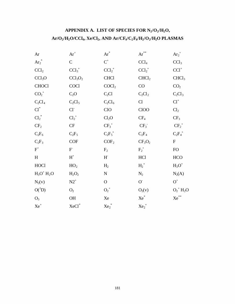
181
APPENDIX A. LIST OF SPECIES FOR N2/O2/H2O,
Ar/O2/H2O/CCl4, Xe/Cl2, AND Ar/CF4/C2F6/H2/O2/H2O PLASMAS
Ar Ar+ Ar* Ar** Ar2+
Ar2* C C+ CCl4 CCl3
CCl2 CCl3+ CCl2
+ CCl2+ CCl+
CCl3O CCl3O2 CHCl CHCl2 CHCl3
CHOCl COCl COCl2 CO CO2
CO2+ C2O C2Cl C2Cl2 C2Cl3
C2Cl4 C2Cl5 C2Cl6 Cl Cl+
Cl* Cl- ClO ClOO Cl2
Cl2* Cl2
+ Cl2O CF4 CF3
CF2 CF CF3+ CF3
- CF2+
C2F6 C2F5 C2F5+ C2F4 C2F4
+
C2F3 COF COF2 CF3O2 F
F+ F- F2 F2+ FO
H H+ H- HCl HCO
HOCl HO2 H2 H2+ H3O
+
H3O+⋅H2O H2O2 N N2 N2(A)
N2(v) N2+ O O- O+
O(1D) O2 O2+ O2(v) O2
+⋅H2O
O3 OH Xe Xe* Xe**
Xe+ XeCl* Xe2* Xe2
+
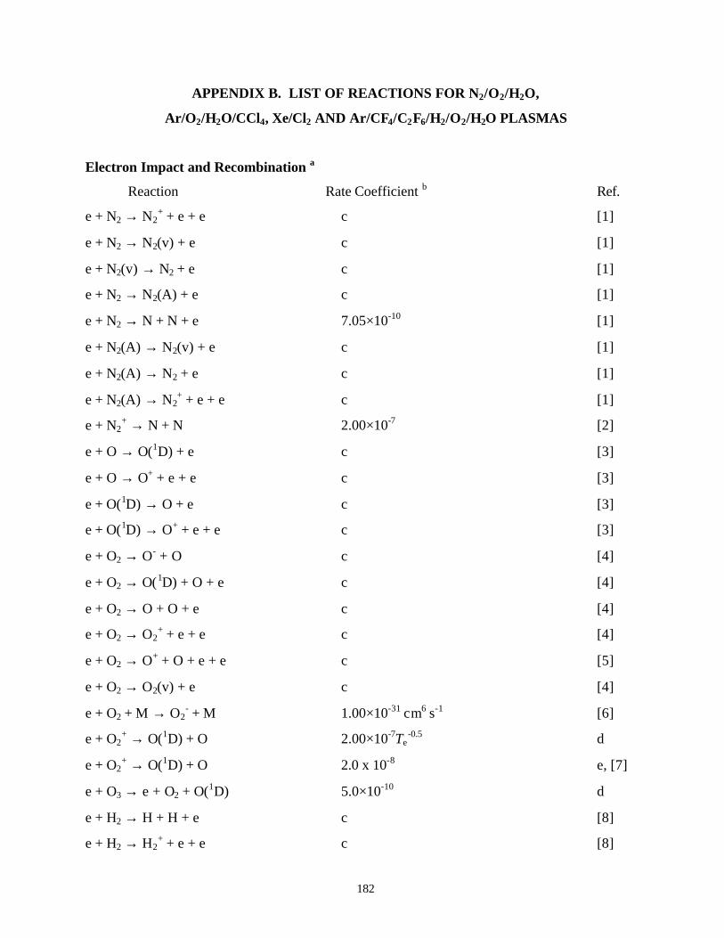
182
APPENDIX B. LIST OF REACTIONS FOR N2/O2/H2O,
Ar/O2/H2O/CCl4, Xe/Cl2 AND Ar/CF4/C2F6/H2/O2/H2O PLASMAS
Electron Impact and Recombination a
Reaction Rate Coefficient b Ref.
e + N2 → N2+ + e + e c [1]
e + N2 → N2(v) + e c [1]
e + N2(v) → N2 + e c [1]
e + N2 → N2(A) + e c [1]
e + N2 → N + N + e 7.05×10⁻¹⁰ [1]
e + N2(A) → N2(v) + e c [1]
e + N2(A) → N2 + e c [1]
e + N2(A) → N2+ + e + e c [1]
e + N2+ → N + N 2.00×10⁻⁷ [2]
e + O → O(1D) + e c [3]
e + O → O+ + e + e c [3]
e + O(1D) → O + e c [3]
e + O(1D) → O+ + e + e c [3]
e + O2 → O- + O c [4]
e + O2 → O(1D) + O + e c [4]
e + O2 → O + O + e c [4]
e + O2 → O2+ + e + e c [4]
e + O2 → O+ + O + e + e c [5]
e + O2 → O2(v) + e c [4]
e + O2 + M → O2- + M 1.00×10⁻³¹ cm6 s-1 [6]
e + O2+ → O(1D) + O 2.00×10⁻⁷Te
-0.5 d
e + O2+ → O(1D) + O 2.0 x 10⁻⁸ e, [7]
e + O3 → e + O2 + O(1D) 5.0×10⁻¹⁰ d
e + H2 → H + H + e c [8]
e + H2 → H2+ + e + e c [8]
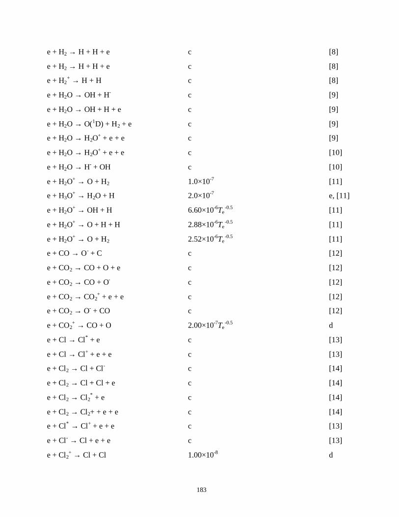
183
e + H2 → H + H + e c [8]
e + H2 → H + H + e c [8]
e + H2+ → H + H c [8]
e + H2O → OH + H- c [9]
e + H2O → OH + H + e c [9]
e + H2O → O(1D) + H2 + e c [9]
e + H2O → H2O+ + e + e c [9]
e + H2O → H2O+ + e + e c [10]
e + H2O → H- + OH c [10]
e + H2O+ → O + H2 1.0×10⁻⁷ [11]
e + H3O+ → H2O + H 2.0×10⁻⁷ e, [11]
e + H2O+ → OH + H 6.60×10⁻⁶Te
-0.5 [11]
e + H2O+ → O + H + H 2.88×10⁻⁶Te
-0.5 [11]
e + H2O+ → O + H2 2.52×10⁻⁶Te
-0.5 [11]
e + CO → O- + C c [12]
e + CO2 → CO + O + e c [12]
e + CO2 → CO + O- c [12]
e + CO2 → CO2+ + e + e c [12]
e + CO2 → O- + CO c [12]
e + CO2+ → CO + O 2.00×10⁻⁷Te
-0.5 d
e + Cl → Cl* + e c [13]
e + Cl → Cl+ + e + e c [13]
e + Cl2 → Cl + Cl- c [14]
e + Cl2 → Cl + Cl + e c [14]
e + Cl2 → Cl2* + e c [14]
e + Cl2 → Cl2+ + e + e c [14]
e + Cl* → Cl+ + e + e c [13]
e + Cl- → Cl + e + e c [13]
e + Cl2+ → Cl + Cl 1.00×10⁻⁸ d
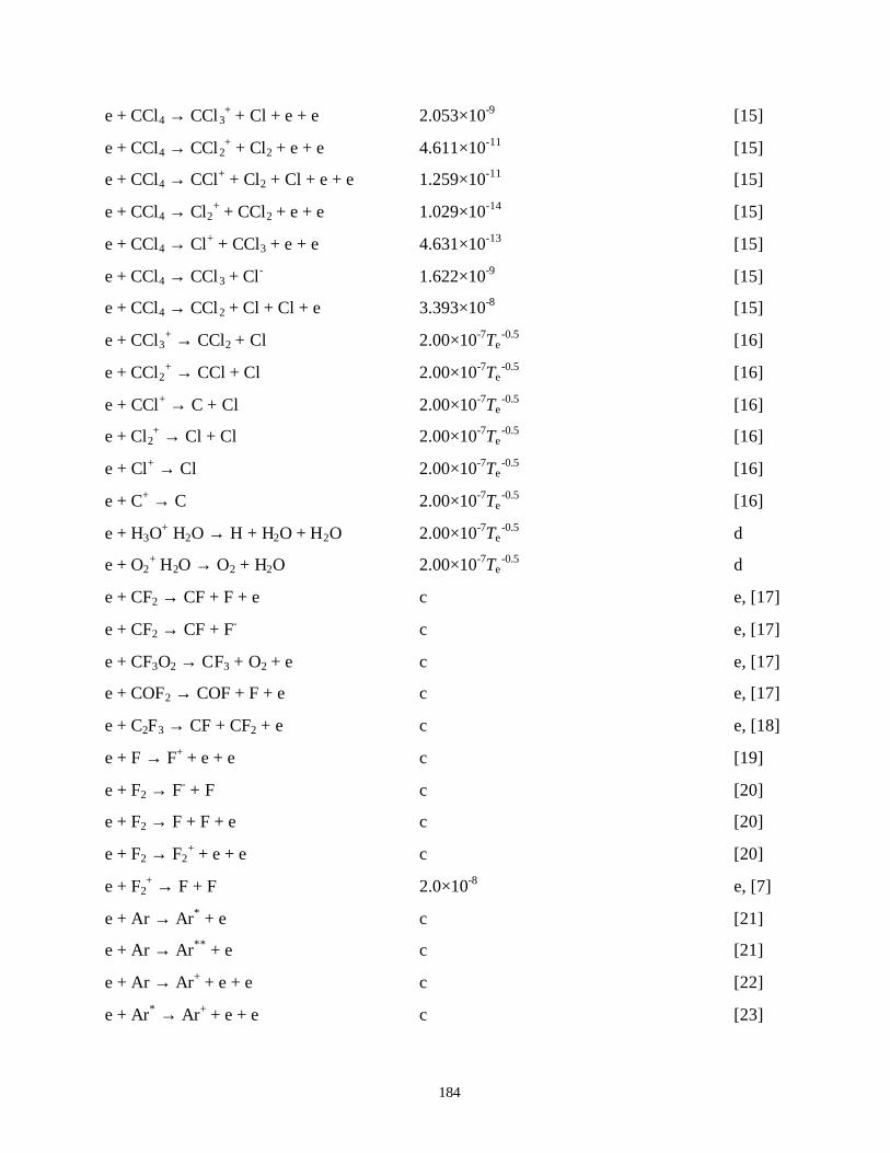
184
e + CCl4 → CCl3+ + Cl + e + e 2.053×10⁻⁹ [15]
e + CCl4 → CCl2+ + Cl2 + e + e 4.611×10⁻¹¹ [15]
e + CCl4 → CCl+ + Cl2 + Cl + e + e 1.259×10⁻¹¹ [15]
e + CCl4 → Cl2+ + CCl2 + e + e 1.029×10⁻¹⁴ [15]
e + CCl4 → Cl+ + CCl3 + e + e 4.631×10⁻¹³ [15]
e + CCl4 → CCl3 + Cl- 1.622×10⁻⁹ [15]
e + CCl4 → CCl2 + Cl + Cl + e 3.393×10⁻⁸ [15]
e + CCl3+ → CCl2 + Cl 2.00×10⁻⁷Te
-0.5 [16]
e + CCl2+ → CCl + Cl 2.00×10⁻⁷Te
-0.5 [16]
e + CCl+ → C + Cl 2.00×10⁻⁷Te-0.5 [16]
e + Cl2+ → Cl + Cl 2.00×10⁻⁷Te
-0.5 [16]
e + Cl+ → Cl 2.00×10⁻⁷Te-0.5 [16]
e + C+ → C 2.00×10⁻⁷Te-0.5 [16]
e + H3O+⋅H2O → H + H2O + H2O 2.00×10⁻⁷Te
-0.5 d
e + O2+⋅H2O → O2 + H2O 2.00×10⁻⁷Te
-0.5 d
e + CF2 → CF + F + e c e, [17]
e + CF2 → CF + F- c e, [17]
e + CF3O2 → CF3 + O2 + e c e, [17]
e + COF2 → COF + F + e c e, [17]
e + C2F3 → CF + CF2 + e c e, [18]
e + F → F+ + e + e c [19]
e + F2 → F- + F c [20]
e + F2 → F + F + e c [20]
e + F2 → F2+ + e + e c [20]
e + F2+ → F + F 2.0×10⁻⁸ e, [7]
e + Ar → Ar* + e c [21]
e + Ar → Ar** + e c [21]
e + Ar → Ar+ + e + e c [22]
e + Ar* → Ar+ + e + e c [23]
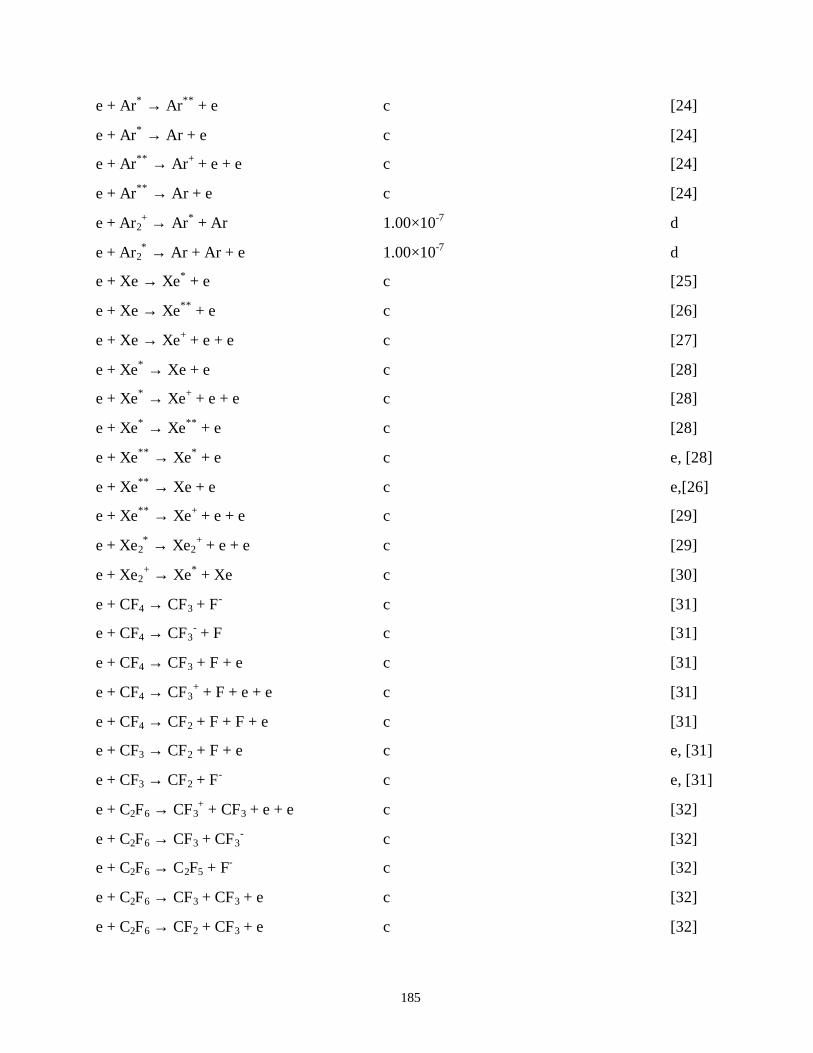
185
e + Ar* → Ar** + e c [24]
e + Ar* → Ar + e c [24]
e + Ar** → Ar+ + e + e c [24]
e + Ar** → Ar + e c [24]
e + Ar2+ → Ar* + Ar 1.00×10⁻⁷ d
e + Ar2* → Ar + Ar + e 1.00×10⁻⁷ d
e + Xe → Xe* + e c [25]
e + Xe → Xe** + e c [26]
e + Xe → Xe+ + e + e c [27]
e + Xe* → Xe + e c [28]
e + Xe* → Xe+ + e + e c [28]
e + Xe* → Xe** + e c [28]
e + Xe** → Xe* + e c e, [28]
e + Xe** → Xe + e c e,[26]
e + Xe** → Xe+ + e + e c [29]
e + Xe2* → Xe2
+ + e + e c [29]
e + Xe2+ → Xe* + Xe c [30]
e + CF4 → CF3 + F- c [31]
e + CF4 → CF3- + F c [31]
e + CF4 → CF3 + F + e c [31]
e + CF4 → CF3+ + F + e + e c [31]
e + CF4 → CF2 + F + F + e c [31]
e + CF3 → CF2 + F + e c e, [31]
e + CF3 → CF2 + F- c e, [31]
e + C2F6 → CF3+ + CF3 + e + e c [32]
e + C2F6 → CF3 + CF3- c [32]
e + C2F6 → C2F5 + F- c [32]
e + C2F6 → CF3 + CF3 + e c [32]
e + C2F6 → CF2 + CF3 + e c [32]
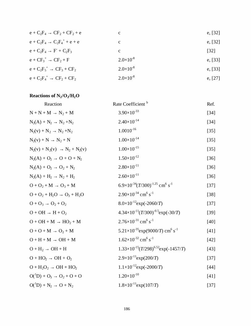
186
e + C2F4 → CF2 + CF2 + e c e, [32]
e + C2F4 → C2F4+ + e + e c e, [32]
e + C2F4 → F- + C2F3 c [32]
e + CF3+ → CF2 + F 2.0×10⁻⁸ e, [33]
e + C2F5+ → CF3 + CF2 2.0×10⁻⁸ e, [33]
e + C2F4+ → CF2 + CF2 2.0×10⁻⁸ e, [27]
Reactions of N2/O2/H2O
Reaction Rate Coefficient b Ref.
N + N + M → N2 + M 3.90×10⁻³³ [34]
N2(A) + N2 → N2 +N2 2.40×10⁻¹⁴ [34]
N2(v) + N2 → N2 +N2 1.0010-16 [35]
N2(v) + N → N2 + N 1.00×10⁻¹⁴ [35]
N2(v) + N2(v) → N2 + N2(v) 1.00×10⁻¹⁵ [35]
N2(A) + O2 → O + O + N2 1.50×10⁻¹² [36]
N2(A) + O2 → O2 + N2 2.80×10⁻¹¹ [36]
N2(A) + H2 → N2 + H2 2.60×10⁻¹¹ [36]
O + O2 + M → O3 + M 6.9×10⁻³⁴(T/300)-1.25 cm6 s-1 [37]
O + O2 + H2O → O3 + H2O 2.90×10⁻³⁴ cm6 s-1 [38]
O + O3 → O2 + O2 8.0×10⁻¹²exp(-2060/T) [37]
O + OH → H + O2 4.34×10⁻¹¹(T/300)-0.5exp(-30/T) [39]
O + OH + M → HO2 + M 2.76×10⁻³¹ cm6 s-1 [40]
O + O + M → O2 + M 5.21×10⁻³⁵exp(9000/T) cm6 s-1 [41]
O + H + M → OH + M 1.62×10⁻³² cm6 s-1 [42]
O + H2 → OH + H 1.33×10⁻¹⁵(T/298)6.52exp(-1457/T) [43]
O + HO2 → OH + O2 2.9×10⁻¹¹exp(200/T) [37]
O + H2O2 → OH + HO2 1.1×10⁻¹²exp(-2000/T) [44]
O(1D) + O3 → O2 + O + O 1.20×10⁻¹⁰ [41]
O(1D) + N2 → O + N2 1.8×10⁻¹¹exp(107/T) [37]
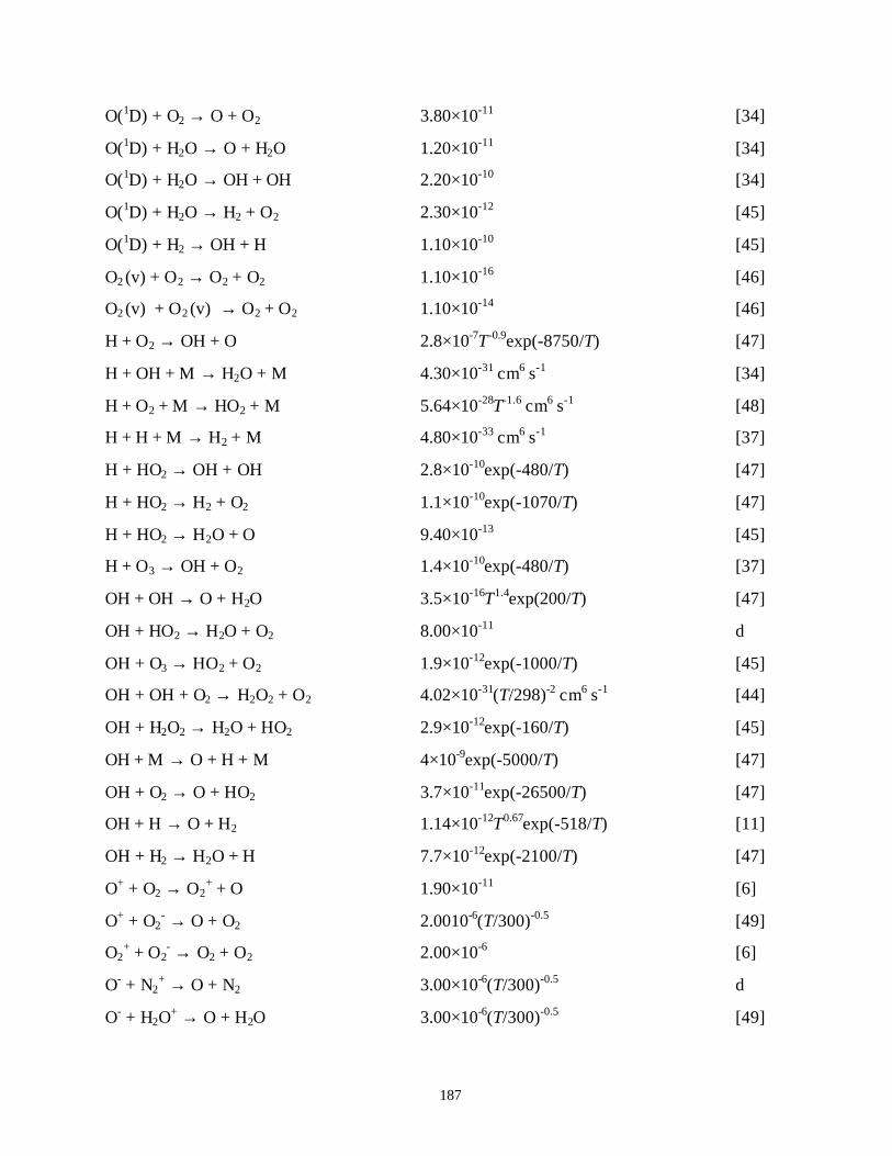
187
O(1D) + O2 → O + O2 3.80×10⁻¹¹ [34]
O(1D) + H2O → O + H2O 1.20×10⁻¹¹ [34]
O(1D) + H2O → OH + OH 2.20×10⁻¹⁰ [34]
O(1D) + H2O → H2 + O2 2.30×10⁻¹² [45]
O(1D) + H2 → OH + H 1.10×10⁻¹⁰ [45]
O2 (v) + O2 → O2 + O2 1.10×10⁻¹⁶ [46]
O2 (v) + O2 (v) → O2 + O2 1.10×10⁻¹⁴ [46]
H + O2 → OH + O 2.8×10⁻⁷T-0.9exp(-8750/T) [47]
H + OH + M → H2O + M 4.30×10⁻³¹ cm6 s-1 [34]
H + O2 + M → HO2 + M 5.64×10⁻²⁸T-1.6 cm6 s-1 [48]
H + H + M → H2 + M 4.80×10⁻³³ cm6 s-1 [37]
H + HO2 → OH + OH 2.8×10⁻¹⁰exp(-480/T) [47]
H + HO2 → H2 + O2 1.1×10⁻¹⁰exp(-1070/T) [47]
H + HO2 → H2O + O 9.40×10⁻¹³ [45]
H + O3 → OH + O2 1.4×10⁻¹⁰exp(-480/T) [37]
OH + OH → O + H2O 3.5×10⁻¹⁶T1.4exp(200/T) [47]
OH + HO2 → H2O + O2 8.00×10⁻¹¹ d
OH + O3 → HO2 + O2 1.9×10⁻¹²exp(-1000/T) [45]
OH + OH + O2 → H2O2 + O2 4.02×10⁻³¹(T/298)-2 cm6 s-1 [44]
OH + H2O2 → H2O + HO2 2.9×10⁻¹²exp(-160/T) [45]
OH + M → O + H + M 4×10⁻⁹exp(-5000/T) [47]
OH + O2 → O + HO2 3.7×10⁻¹¹exp(-26500/T) [47]
OH + H → O + H2 1.14×10⁻¹²T0.67exp(-518/T) [11]
OH + H2 → H2O + H 7.7×10⁻¹²exp(-2100/T) [47]
O+ + O2 → O2+ + O 1.90×10⁻¹¹ [6]
O+ + O2- → O + O2 2.0010-6(T/300)-0.5 [49]
O2+ + O2
- → O2 + O2 2.00×10⁻⁶ [6]
O- + N2+ → O + N2 3.00×10⁻⁶(T/300)-0.5 d
O- + H2O+ → O + H2O 3.00×10⁻⁶(T/300)-0.5 [49]
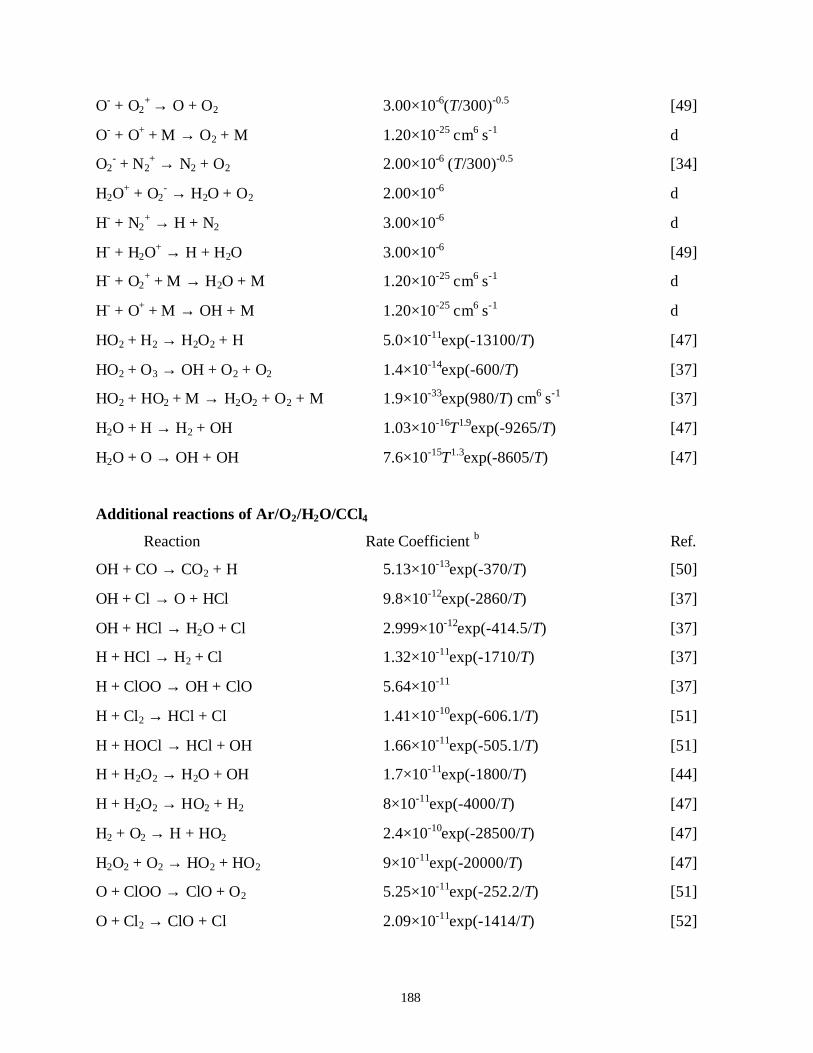
188
O- + O2+ → O + O2 3.00×10⁻⁶(T/300)-0.5 [49]
O- + O+ + M → O2 + M 1.20×10⁻²⁵ cm6 s-1 d
O2- + N2
+ → N2 + O2 2.00×10⁻⁶ (T/300)-0.5 [34]
H2O+ + O2
- → H2O + O2 2.00×10⁻⁶ d
H- + N2+ → H + N2 3.00×10⁻⁶ d
H- + H2O+ → H + H2O 3.00×10⁻⁶ [49]
H- + O2+ + M → H2O + M 1.20×10⁻²⁵ cm6 s-1 d
H- + O+ + M → OH + M 1.20×10⁻²⁵ cm6 s-1 d
HO2 + H2 → H2O2 + H 5.0×10⁻¹¹exp(-13100/T) [47]
HO2 + O3 → OH + O2 + O2 1.4×10⁻¹⁴exp(-600/T) [37]
HO2 + HO2 + M → H2O2 + O2 + M 1.9×10⁻³³exp(980/T) cm6 s-1 [37]
H2O + H → H2 + OH 1.03×10⁻¹⁶T1.9exp(-9265/T) [47]
H2O + O → OH + OH 7.6×10⁻¹⁵T1.3exp(-8605/T) [47]
Additional reactions of Ar/O2/H2O/CCl4
Reaction Rate Coefficient b Ref.
OH + CO → CO2 + H 5.13×10⁻¹³exp(-370/T) [50]
OH + Cl → O + HCl 9.8×10⁻¹²exp(-2860/T) [37]
OH + HCl → H2O + Cl 2.999×10⁻¹²exp(-414.5/T) [37]
H + HCl → H2 + Cl 1.32×10⁻¹¹exp(-1710/T) [37]
H + ClOO → OH + ClO 5.64×10⁻¹¹ [37]
H + Cl2 → HCl + Cl 1.41×10⁻¹⁰exp(-606.1/T) [51]
H + HOCl → HCl + OH 1.66×10⁻¹¹exp(-505.1/T) [51]
H + H2O2 → H2O + OH 1.7×10⁻¹¹exp(-1800/T) [44]
H + H2O2 → HO2 + H2 8×10-11exp(-4000/T) [47]
H2 + O2 → H + HO2 2.4×10⁻¹⁰exp(-28500/T) [47]
H2O2 + O2 → HO2 + HO2 9×10-11exp(-20000/T) [47]
O + ClOO → ClO + O2 5.25×10⁻¹¹exp(-252.2/T) [51]
O + Cl2 → ClO + Cl 2.09×10⁻¹¹exp(-1414/T) [52]
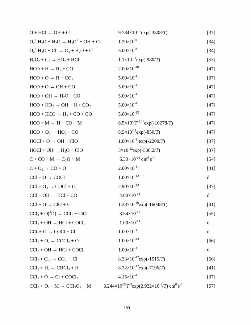
189
O + HCl → OH + Cl 9.784×10⁻¹²exp(-3308/T) [37]
O2+⋅H2O + H2O → H3O
+ + OH + O2 1.20×10⁻⁹ [34]
O2+⋅H2O + Cl- → O2 + H2O + Cl 5.00×10⁻⁸ [34]
H2O2 + Cl → HO2 + HCl 1.1×10⁻¹¹exp(-980/T) [53]
HCO + H → H2 + CO 2.00×10⁻¹⁰ [47]
HCO + O → H + CO2 5.00×10⁻¹¹ [37]
HCO + O → OH + CO 5.00×10⁻¹¹ [47]
HCO + OH → H2O + CO 5.00×10⁻¹¹ [47]
HCO + HO2 → OH + H + CO2 5.00×10⁻¹¹ [47]
HCO + HCO → H2 + CO + CO 5.00×10⁻¹² [47]
HCO + M → H + CO + M 8.5×10⁻³T-2.14exp(-10278/T) [47]
HCO + O2 → HO2 + CO 8.5×10⁻¹¹exp(-850/T) [47]
HOCl + O → OH + ClO 1.00×10⁻¹¹exp(-2200/T) [37]
HOCl + OH → H2O + ClO 3×10-12exp(-500.2/T) [37]
C + CO + M → C2O + M 6.30×10⁻³² cm6 s-1 [54]
C + O2 → CO + O 2.60×10⁻¹¹ [41]
CCl + O → COCl 1.00×10⁻¹² d
CCl + O2 → COCl + O 2.90×10⁻¹² [37]
CCl + OH → HCl + CO 4.00×10⁻¹¹ d
CCl + O → ClO + C 1.38×10⁻¹⁰exp(-16048/T) [41]
CCl4 + O(1D) → CCl3 + ClO 3.54×10⁻¹⁰ [55]
CCl3 + OH → HCl + COCl2 1.00×10⁻¹¹ d
CCl2+ O → COCl + Cl 1.00×10⁻¹¹ d
CCl2 + O2 → COCl2 + O 1.00×10⁻¹³ [56]
CCl2 + OH → HCl + COCl 1.00×10⁻¹¹ d
CCl2 + Cl2 → CCl3 + Cl 8.33×10⁻¹²exp(-1515/T) [56]
CCl3 + H2 → CHCl3 + H 8.32×10⁻¹²exp(-7196/T) [41]
CCl3 + O → Cl + COCl2 4.15×10⁻¹¹ [37]
CCl3 + O2 + M → CCl3O2 + M 3.244×10⁻²³T-3exp(2.922×10⁻⁸/T) cm6 s-1 [57]
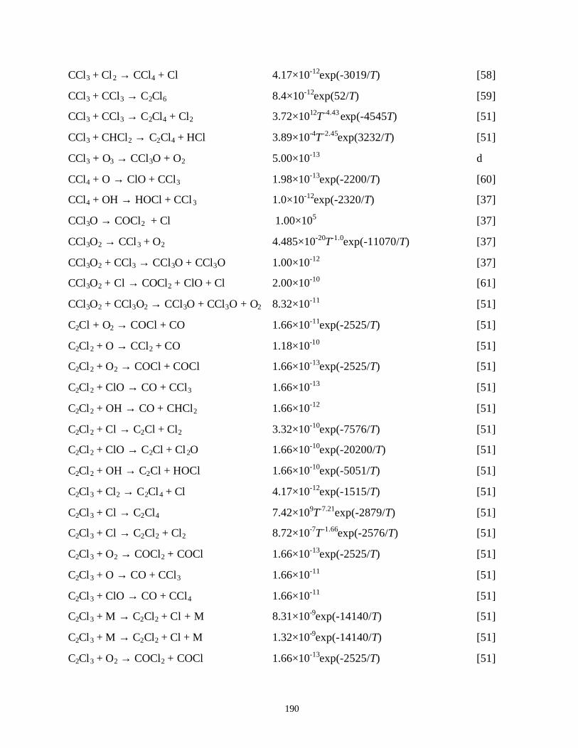
190
CCl3 + Cl2 → CCl4 + Cl 4.17×10⁻¹²exp(-3019/T) [58]
CCl3 + CCl3 → C2Cl6 8.4×10⁻¹²exp(52/T) [59]
CCl3 + CCl3 → C2Cl4 + Cl2 3.72×10¹²T-4.43 exp(-4545T) [51]
CCl3 + CHCl2 → C2Cl4 + HCl 3.89×10⁻⁴T-2.45exp(3232/T) [51]
CCl3 + O3 → CCl3O + O2 5.00×10⁻¹³ d
CCl4 + O → ClO + CCl3 1.98×10⁻¹³exp(-2200/T) [60]
CCl4 + OH → HOCl + CCl3 1.0×10⁻¹²exp(-2320/T) [37]
CCl3O → COCl2 + Cl 1.00×10⁵ [37]
CCl3O2 → CCl3 + O2 4.485×10⁻²⁰T-1.0exp(-11070/T) [37]
CCl3O2 + CCl3 → CCl3O + CCl3O 1.00×10⁻¹² [37]
CCl3O2 + Cl → COCl2 + ClO + Cl 2.00×10⁻¹⁰ [61]
CCl3O2 + CCl3O2 → CCl3O + CCl3O + O2 8.32×10⁻¹¹ [51]
C2Cl + O2 → COCl + CO 1.66×10⁻¹¹exp(-2525/T) [51]
C2Cl2 + O → CCl2 + CO 1.18×10⁻¹⁰ [51]
C2Cl2 + O2 → COCl + COCl 1.66×10⁻¹³exp(-2525/T) [51]
C2Cl2 + ClO → CO + CCl3 1.66×10⁻¹³ [51]
C2Cl2 + OH → CO + CHCl2 1.66×10⁻¹² [51]
C2Cl2 + Cl → C2Cl + Cl2 3.32×10⁻¹⁰exp(-7576/T) [51]
C2Cl2 + ClO → C2Cl + Cl2O 1.66×10⁻¹⁰exp(-20200/T) [51]
C2Cl2 + OH → C2Cl + HOCl 1.66×10⁻¹⁰exp(-5051/T) [51]
C2Cl3 + Cl2 → C2Cl4 + Cl 4.17×10⁻¹²exp(-1515/T) [51]
C2Cl3 + Cl → C2Cl4 7.42×10⁹T-7.21exp(-2879/T) [51]
C2Cl3 + Cl → C2Cl2 + Cl2 8.72×10⁻⁷T-1.66exp(-2576/T) [51]
C2Cl3 + O2 → COCl2 + COCl 1.66×10⁻¹³exp(-2525/T) [51]
C2Cl3 + O → CO + CCl3 1.66×10⁻¹¹ [51]
C2Cl3 + ClO → CO + CCl4 1.66×10⁻¹¹ [51]
C2Cl3 + M → C2Cl2 + Cl + M 8.31×10⁻⁹exp(-14140/T) [51]
C2Cl3 + M → C2Cl2 + Cl + M 1.32×10⁻⁹exp(-14140/T) [51]
C2Cl3 + O2 → COCl2 + COCl 1.66×10⁻¹³exp(-2525/T) [51]
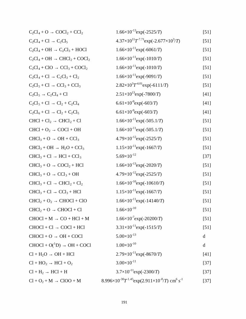
191
C2Cl4 + O → COCl2 + CCl2 1.66×10⁻¹³exp(-2525/T) [51]
C2Cl4 + Cl → C2Cl5 4.37×10¹¹T-7.71exp(-2.677×10³/T) [51]
C2Cl4 + OH → C2Cl3 + HOCl 1.66×10⁻¹¹exp(-6061/T) [51]
C2Cl4 + OH → CHCl2 + COCl2 1.66×10⁻¹¹exp(-1010/T) [51]
C2Cl4 + ClO → CCl3 + COCl2 1.66×10⁻¹¹exp(-1010/T) [51]
C2Cl4 + Cl → C2Cl3 + Cl2 1.66×10⁻¹¹exp(-9091/T) [51]
C2Cl5 + Cl → CCl3 + CCl3 2.82×10³T-4.01exp(-6111/T) [51]
C2Cl5 → C2Cl4 + Cl 2.51×10¹³exp(-7800/T) [41]
C2Cl5 + Cl → Cl2 + C2Cl4 6.61×10⁻⁹exp(-603/T) [41]
C2Cl6 + Cl → Cl2 + C2Cl5 6.61×10⁻⁹exp(-603/T) [41]
CHCl + Cl2 → CHCl2 + Cl 1.66×10⁻¹¹exp(-505.1/T) [51]
CHCl + O2 → COCl + OH 1.66×10⁻¹¹exp(-505.1/T) [51]
CHCl3 + O → OH + CCl3 4.79×10⁻¹²exp(-2525/T) [51]
CHCl3 + OH → H2O + CCl3 1.15×10⁻¹¹exp(-1667/T) [51]
CHCl3 + Cl → HCl + CCl3 5.69×10⁻¹² [37]
CHCl3 + O → COCl2 + HCl 1.66×10⁻¹³exp(-2020/T) [51]
CHCl3 + O → CCl3 + OH 4.79×10⁻¹²exp(-2525/T) [51]
CHCl3 + Cl → CHCl2 + Cl2 1.66×10⁻¹⁰exp(-10610/T) [51]
CHCl3 + Cl → CCl3 + HCl 1.15×10⁻¹¹exp(-1667/T) [51]
CHCl2 + O2 → CHOCl + ClO 1.66×10⁻¹¹exp(-14140/T) [51]
CHCl2 + O → CHOCl + Cl 1.66×10⁻¹⁰ [51]
CHOCl + M → CO + HCl + M 1.66×10⁻⁷exp(-20200/T) [51]
CHOCl + Cl → COCl + HCl 3.31×10⁻¹¹exp(-1515/T) [51]
CHOCl + O → OH + COCl 5.00×10⁻¹³ d
CHOCl + O(1D) → OH + COCl 1.00×10⁻¹⁰ d
Cl + H2O → OH + HCl 2.79×10⁻¹¹exp(-8670/T) [41]
Cl + HO2 → HCl + O2 3.00×10⁻¹¹ [37]
Cl + H2 → HCl + H 3.7×10⁻¹¹exp(-2300/T) [37]
Cl + O2 + M → ClOO + M 8.996×10⁻³⁰T-1.45exp(2.911×10⁻⁸/T) cm6 s-1 [37]
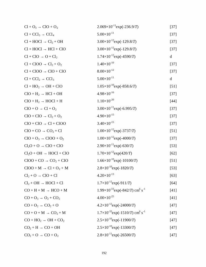
192
Cl + O3 → ClO + O2 2.069×10⁻¹¹exp(-236.9/T) [37]
Cl + CCl3 → CCl4 5.00×10⁻¹¹ [37]
Cl + HOCl → Cl2 + OH 3.00×10⁻¹²exp(-129.8/T) [37]
Cl + HOCl → HCl + ClO 3.00×10⁻¹²exp(-129.8/T) [37]
Cl + ClO → O + Cl2 1.74×10⁻¹²exp(-4590/T) d
Cl + ClOO → Cl2 + O2 1.40×10⁻¹⁰ [37]
Cl + ClOO → ClO + ClO 8.00×10⁻¹² [37]
Cl + CCl2 → CCl3 5.00×10⁻¹¹ d
Cl + HO2 → OH + ClO 1.05×10⁻¹⁰exp(-858.6/T) [51]
ClO + H2 → HCl + OH 4.98×10⁻¹⁶ [37]
ClO + H2 → HOCl + H 1.10×10⁻²⁰ [44]
ClO + O → Cl + O2 3.00×10⁻¹¹exp(-6.995/T) [37]
ClO + ClO → Cl2 + O2 4.90×10⁻¹⁵ [37]
ClO + ClO → Cl + ClOO 3.40×10⁻¹⁵ [37]
ClO + CO → CO2 + Cl 1.00×10⁻¹²exp(-3737/T) [51]
ClO + O3 → ClOO + O2 1.00×10⁻¹²exp(-4000/T) [37]
Cl2O + O → ClO + ClO 2.90×10⁻¹¹exp(-630/T) [53]
Cl2O + OH → HOCl + ClO 1.70×10⁻¹²exp(420/T) [62]
ClOO + CO → CO2 + CIO 1.66×10⁻¹⁰exp(-10100/T) [51]
ClOO + M → Cl + O2 + M 2.8×10⁻¹⁰exp(-1820/T) [53]
Cl2 + O → ClO + Cl 4.20×10⁻¹³ [63]
Cl2 + OH → HOCl + Cl 1.7×10⁻¹²exp(-911/T) [64]
CO + H + M → HCO + M 1.99×10⁻³³exp(-842/T) cm6 s-1 [41]
CO + O3 → O2 + CO2 4.00×10⁻²⁵ [41]
CO + O2 → CO2 + O 4.2×10⁻¹²exp(-24000/T) [47]
CO + O + M → CO2 + M 1.7×10⁻³³exp(-1510/T) cm6 s-1 [47]
CO + HO2 → OH + CO2 2.5×10⁻¹⁰exp(-11900/T) [47]
CO2 + H → CO + OH 2.5×10⁻¹⁰exp(-13300/T) [47]
CO2 + O → CO + O2 2.8×10⁻¹¹exp(-26500/T) [47]
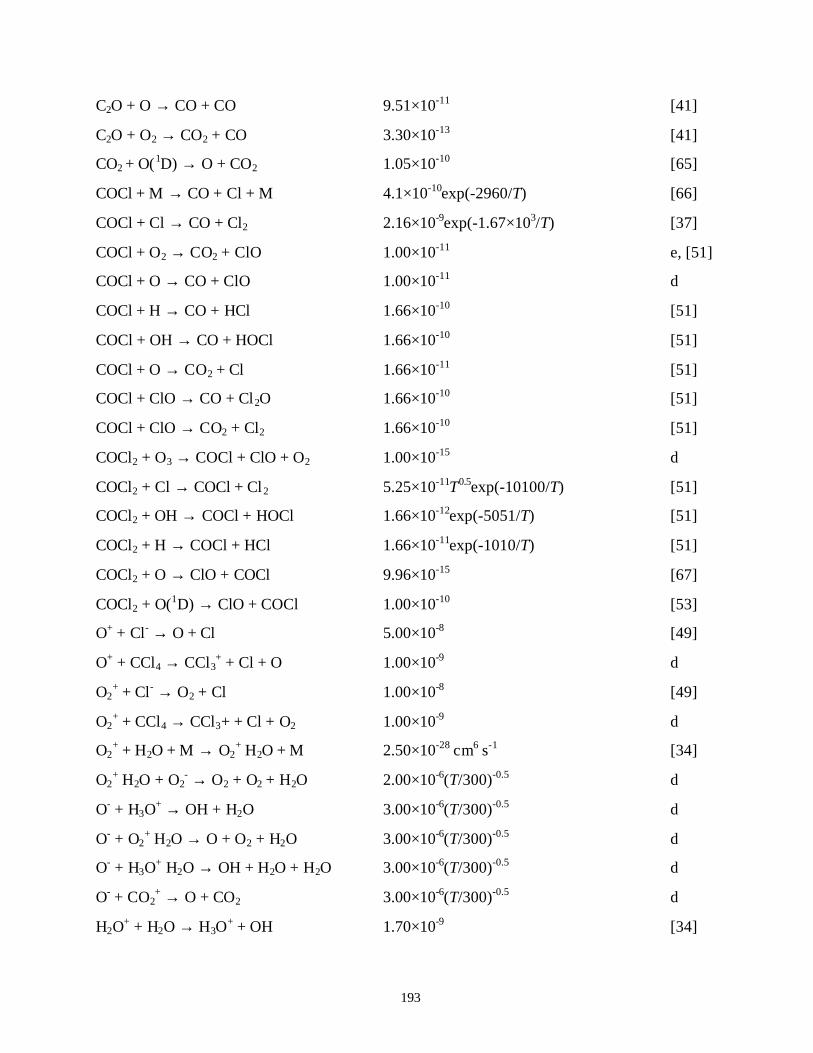
193
C2O + O → CO + CO 9.51×10⁻¹¹ [41]
C2O + O2 → CO2 + CO 3.30×10⁻¹³ [41]
CO2 + O(1D) → O + CO2 1.05×10⁻¹⁰ [65]
COCl + M → CO + Cl + M 4.1×10⁻¹⁰exp(-2960/T) [66]
COCl + Cl → CO + Cl2 2.16×10⁻⁹exp(-1.67×10³/T) [37]
COCl + O2 → CO2 + ClO 1.00×10⁻¹¹ e, [51]
COCl + O → CO + ClO 1.00×10⁻¹¹ d
COCl + H → CO + HCl 1.66×10⁻¹⁰ [51]
COCl + OH → CO + HOCl 1.66×10⁻¹⁰ [51]
COCl + O → CO2 + Cl 1.66×10⁻¹¹ [51]
COCl + ClO → CO + Cl2O 1.66×10⁻¹⁰ [51]
COCl + ClO → CO2 + Cl2 1.66×10⁻¹⁰ [51]
COCl2 + O3 → COCl + ClO + O2 1.00×10⁻¹⁵ d
COCl2 + Cl → COCl + Cl2 5.25×10⁻¹¹T0.5exp(-10100/T) [51]
COCl2 + OH → COCl + HOCl 1.66×10⁻¹²exp(-5051/T) [51]
COCl2 + H → COCl + HCl 1.66×10⁻¹¹exp(-1010/T) [51]
COCl2 + O → ClO + COCl 9.96×10⁻¹⁵ [67]
COCl2 + O(1D) → ClO + COCl 1.00×10⁻¹⁰ [53]
O+ + Cl- → O + Cl 5.00×10⁻⁸ [49]
O+ + CCl4 → CCl3+ + Cl + O 1.00×10⁻⁹ d
O2+ + Cl- → O2 + Cl 1.00×10⁻⁸ [49]
O2+ + CCl4 → CCl3+ + Cl + O2 1.00×10⁻⁹ d
O2+ + H2O + M → O2
+⋅H2O + M 2.50×10⁻²⁸ cm6 s-1 [34]
O2+⋅H2O + O2
- → O2 + O2 + H2O 2.00×10⁻⁶(T/300)-0.5 d
O- + H3O+ → OH + H2O 3.00×10⁻⁶(T/300)-0.5 d
O- + O2+⋅H2O → O + O2 + H2O 3.00×10⁻⁶(T/300)-0.5 d
O- + H3O+⋅H2O → OH + H2O + H2O 3.00×10⁻⁶(T/300)-0.5 d
O- + CO2+ → O + CO2 3.00×10⁻⁶(T/300)-0.5 d
H2O+ + H2O → H3O
+ + OH 1.70×10⁻⁹ [34]
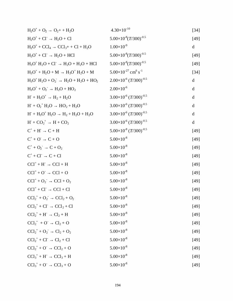
194
H2O+ + O2 → O2+ + H2O 4.30×10⁻¹⁰ [34]
H2O+ + Cl- → H2O + Cl 5.00×10⁻⁸(T/300)-0.5 [49]
H2O+ + CCl4 → CCl3+ + Cl + H2O 1.00×10⁻⁹ d
H3O+ + Cl- → H2O + HCl 5.00×10⁻⁸(T/300)-0.5 [49]
H3O+⋅H2O + Cl- → H2O + H2O + HCl 5.00×10⁻⁸(T/300)-0.5 [49]
H3O+ + H2O + M → H3O
+⋅H2O + M 5.00×10⁻²⁷ cm6 s-1 [34]
H3O+⋅H2O + O2
- → H2O + H2O + HO2 2.00×10⁻⁶ (T/300)-0.5 d
H3O+ + O2
- → H2O + HO2 2.00×10⁻⁶ d
H- + H3O+ → H2 + H2O 3.00×10⁻⁶ (T/300)-0.5 d
H- + O2+⋅H2O → HO2 + H2O 3.00×10⁻⁶ (T/300)-0.5 d
H- + H3O+⋅H2O → H2 + H2O + H2O 3.00×10⁻⁶ (T/300)-0.5 d
H- + CO2+ → H + CO2 3.00×10⁻⁶ (T/300)-0.5 d
C+ + H- → C + H 5.00×10⁻⁸ (T/300)-0.5 [49]
C+ + O- → C + O 5.00×10⁻⁸ [49]
C+ + O2- → C + O2 5.00×10⁻⁸ [49]
C+ + Cl- → C + Cl 5.00×10⁻⁸ [49]
CCl+ + H- → CCl + H 5.00×10⁻⁸ [49]
CCl+ + O- → CCl + O 5.00×10⁻⁸ [49]
CCl+ + O2- → CCl + O2 5.00×10⁻⁸ [49]
CCl+ + Cl- → CCl + Cl 5.00×10⁻⁸ [49]
CCl2+ + O2
- → CCl2 + O2 5.00×10⁻⁸ [49]
CCl2+ + Cl- → CCl2 + Cl 5.00×10⁻⁸ [49]
CCl2+ + H- → Cl2 + H 5.00×10⁻⁸ [49]
CCl2+ + O- → Cl2 + O 5.00×10⁻⁸ [49]
CCl2+ + O2
- → Cl2 + O2 5.00×10⁻⁸ [49]
CCl2+ + Cl- → Cl2 + Cl 5.00×10⁻⁸ [49]
CCl2+ + O- → CCl2 + O 5.00×10⁻⁸ [49]
CCl3+ + H- → CCl3 + H 5.00×10⁻⁸ [49]
CCl3+ + O- → CCl3 + O 5.00×10⁻⁸ [49]
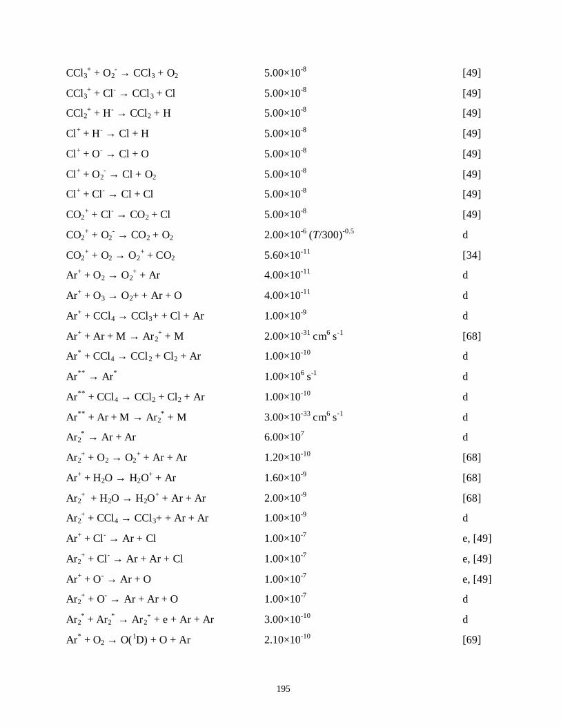
195
CCl3+ + O2
- → CCl3 + O2 5.00×10⁻⁸ [49]
CCl3+ + Cl- → CCl3 + Cl 5.00×10⁻⁸ [49]
CCl2+ + H- → CCl2 + H 5.00×10⁻⁸ [49]
Cl+ + H- → Cl + H 5.00×10⁻⁸ [49]
Cl+ + O- → Cl + O 5.00×10⁻⁸ [49]
Cl+ + O2- → Cl + O2 5.00×10⁻⁸ [49]
Cl+ + Cl- → Cl + Cl 5.00×10⁻⁸ [49]
CO2+ + Cl- → CO2 + Cl 5.00×10⁻⁸ [49]
CO2+ + O2
- → CO2 + O2 2.00×10⁻⁶ (T/300)-0.5 d
CO2+ + O2 → O2
+ + CO2 5.60×10⁻¹¹ [34]
Ar+ + O2 → O2+ + Ar 4.00×10⁻¹¹ d
Ar+ + O3 → O2+ + Ar + O 4.00×10⁻¹¹ d
Ar+ + CCl4 → CCl3+ + Cl + Ar 1.00×10⁻⁹ d
Ar+ + Ar + M → Ar2+ + M 2.00×10⁻³¹ cm6 s-1 [68]
Ar* + CCl4 → CCl2 + Cl2 + Ar 1.00×10⁻¹⁰ d
Ar** → Ar* 1.00×10⁶ s-1 d
Ar** + CCl4 → CCl2 + Cl2 + Ar 1.00×10⁻¹⁰ d
Ar** + Ar + M → Ar2* + M 3.00×10⁻³³ cm6 s-1 d
Ar2* → Ar + Ar 6.00×10⁷ d
Ar2+ + O2 → O2
+ + Ar + Ar 1.20×10⁻¹⁰ [68]
Ar+ + H2O → H2O+ + Ar 1.60×10⁻⁹ [68]
Ar2+ + H2O → H2O
+ + Ar + Ar 2.00×10⁻⁹ [68]
Ar2+ + CCl4 → CCl3+ + Ar + Ar 1.00×10⁻⁹ d
Ar+ + Cl- → Ar + Cl 1.00×10⁻⁷ e, [49]
Ar2+ + Cl- → Ar + Ar + Cl 1.00×10⁻⁷ e, [49]
Ar+ + O- → Ar + O 1.00×10⁻⁷ e, [49]
Ar2+ + O- → Ar + Ar + O 1.00×10⁻⁷ d
Ar2* + Ar2
* → Ar2+ + e + Ar + Ar 3.00×10⁻¹⁰ d
Ar* + O2 → O(1D) + O + Ar 2.10×10⁻¹⁰ [69]
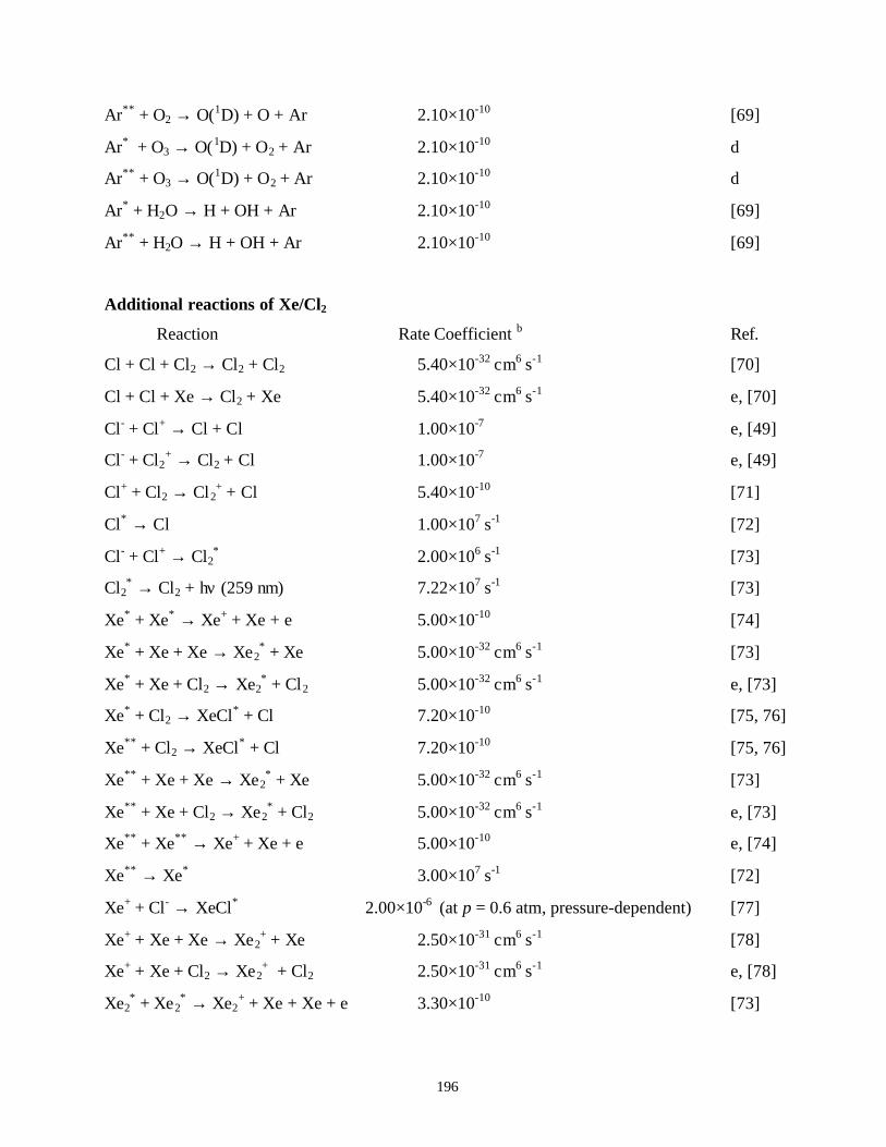
196
Ar** + O2 → O(1D) + O + Ar 2.10×10⁻¹⁰ [69]
Ar* + O3 → O(1D) + O2 + Ar 2.10×10⁻¹⁰ d
Ar** + O3 → O(1D) + O2 + Ar 2.10×10⁻¹⁰ d
Ar* + H2O → H + OH + Ar 2.10×10⁻¹⁰ [69]
Ar** + H2O → H + OH + Ar 2.10×10⁻¹⁰ [69]
Additional reactions of Xe/Cl2
Reaction Rate Coefficient b Ref.
Cl + Cl + Cl2 → Cl2 + Cl2 5.40×10⁻³² cm6 s-1 [70]
Cl + Cl + Xe → Cl2 + Xe 5.40×10⁻³² cm6 s-1 e, [70]
Cl- + Cl+ → Cl + Cl 1.00×10⁻⁷ e, [49]
Cl- + Cl2+ → Cl2 + Cl 1.00×10⁻⁷ e, [49]
Cl+ + Cl2 → Cl2+ + Cl 5.40×10⁻¹⁰ [71]
Cl* → Cl 1.00×10⁷ s-1 [72]
Cl- + Cl+ → Cl2* 2.00×106 s-1 [73]
Cl2* → Cl2 + hν (259 nm) 7.22×10⁷ s-1 [73]
Xe* + Xe* → Xe+ + Xe + e 5.00×10⁻¹⁰ [74]
Xe* + Xe + Xe → Xe2* + Xe 5.00×10⁻³² cm6 s-1 [73]
Xe* + Xe + Cl2 → Xe2* + Cl2 5.00×10⁻³² cm6 s-1 e, [73]
Xe* + Cl2 → XeCl* + Cl 7.20×10⁻¹⁰ [75, 76]
Xe** + Cl2 → XeCl* + Cl 7.20×10⁻¹⁰ [75, 76]
Xe** + Xe + Xe → Xe2* + Xe 5.00×10⁻³² cm6 s-1 [73]
Xe** + Xe + Cl2 → Xe2* + Cl2 5.00×10⁻³² cm6 s-1 e, [73]
Xe** + Xe** → Xe+ + Xe + e 5.00×10⁻¹⁰ e, [74]
Xe** → Xe* 3.00×10⁷ s-1 [72]
Xe+ + Cl- → XeCl* 2.00×10⁻⁶ (at p = 0.6 atm, pressure-dependent) [77]
Xe+ + Xe + Xe → Xe2+ + Xe 2.50×10⁻³¹ cm6 s-1 [78]
Xe+ + Xe + Cl2 → Xe2+ + Cl2 2.50×10⁻³¹ cm6 s-1 e, [78]
Xe2* + Xe2
* → Xe2+ + Xe + Xe + e 3.30×10⁻¹⁰ [73]
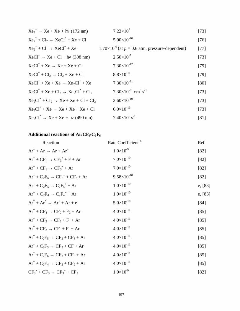
197
Xe2* → Xe + Xe + hν (172 nm) 7.22×10⁷ [73]
Xe2* + Cl2 → XeCl* + Xe + Cl 5.00×10⁻¹⁰ [76]
Xe2+ + Cl- → XeCl* + Xe 1.70×10⁻⁶ (at p = 0.6 atm, pressure-dependent) [77]
XeCl* → Xe + Cl + hν (308 nm) 2.50×10⁻⁷ [73]
XeCl* + Xe → Xe + Xe + Cl 7.30×10⁻¹² [79]
XeCl* + Cl2 → Cl2 + Xe + Cl 8.8×10⁻¹¹ [79]
XeCl* + Xe + Xe → Xe2Cl* + Xe 7.30×10⁻³¹ [80]
XeCl* + Xe + Cl2 → Xe2Cl* + Cl2 7.30×10⁻³¹ cm6 s-1 [73]
Xe2Cl* + Cl2 → Xe + Xe + Cl + Cl2 2.60×10⁻¹⁰ [73]
Xe2Cl* + Xe → Xe + Xe + Xe + Cl 6.0×10⁻¹⁵ [73]
Xe2Cl* → Xe + Xe + hν (490 nm) 7.40×10⁶ s-1 [81]
Additional reactions of Ar/CF4/C2F6
Reaction Rate Coefficient b Ref.
Ar+ + Ar → Ar + Ar+ 1.0×10⁻⁹ [82]
Ar+ + CF4 → CF3+ + F + Ar 7.0×10⁻¹⁰ [82]
Ar+ + CF3 → CF3+ + Ar 7.0×10⁻¹⁰ [82]
Ar+ + C2F6 → CF3+ + CF3 + Ar 9.58×10⁻¹⁰ [82]
Ar+ + C2F5 → C2F5+ + Ar 1.0×10⁻¹⁰ e, [83]
Ar+ + C2F4 → C2F4+ + Ar 1.0×10⁻¹⁰ e, [83]
Ar* + Ar* → Ar+ + Ar + e 5.0×10⁻¹⁰ [84]
Ar* + CF4 → CF2 + F2 + Ar 4.0×10⁻¹¹ [85]
Ar* + CF3 → CF2 + F + Ar 4.0×10⁻¹¹ [85]
Ar* + CF2 → CF + F + Ar 4.0×10⁻¹¹ [85]
Ar* + C2F5 → CF2 + CF3 + Ar 4.0×10⁻¹¹ [85]
Ar* + C2F3 → CF2 + CF + Ar 4.0×10⁻¹¹ [85]
Ar* + C2F6 → CF3 + CF3 + Ar 4.0×10⁻¹¹ [85]
Ar* + C2F4 → CF2 + CF2 + Ar 4.0×10⁻¹¹ [85]
CF3+ + CF3 → CF3
+ + CF3 1.0×10⁻⁹ [82]
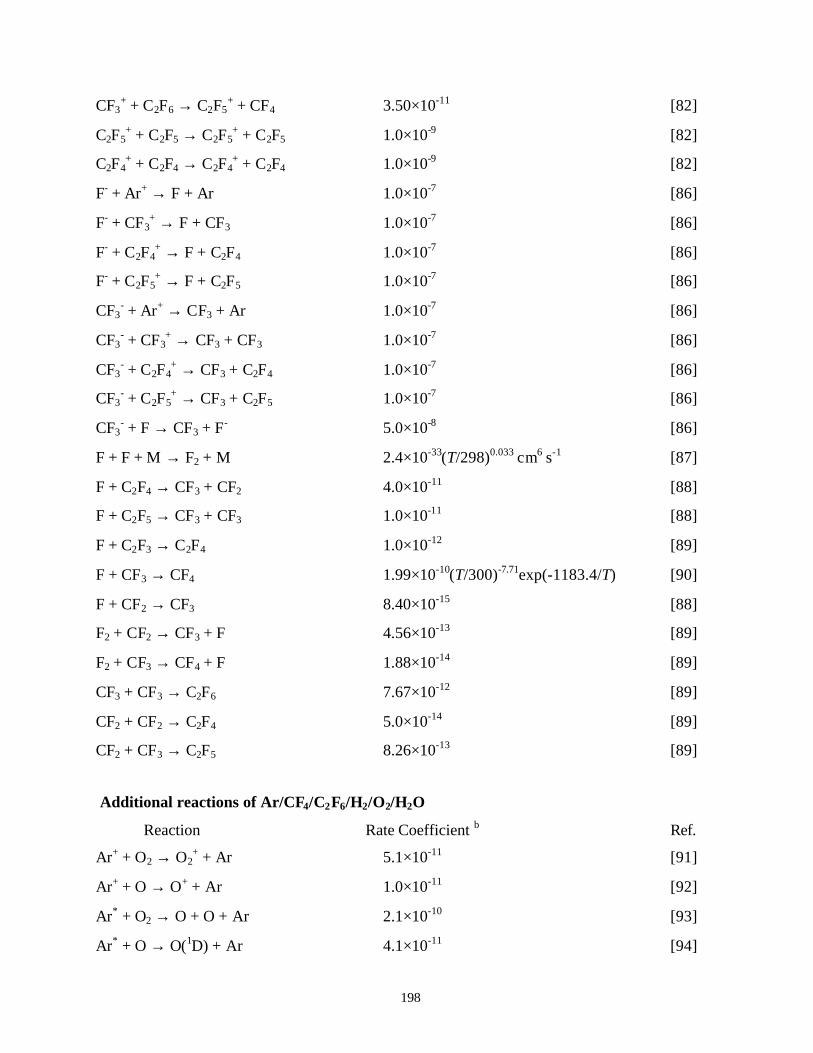
198
CF3+ + C2F6 → C2F5
+ + CF4 3.50×10⁻¹¹ [82]
C2F5+ + C2F5 → C2F5
+ + C2F5 1.0×10⁻⁹ [82]
C2F4+ + C2F4 → C2F4
+ + C2F4 1.0×10⁻⁹ [82]
F- + Ar+ → F + Ar 1.0×10⁻⁷ [86]
F- + CF3+ → F + CF3 1.0×10⁻⁷ [86]
F- + C2F4+ → F + C2F4 1.0×10⁻⁷ [86]
F- + C2F5+ → F + C2F5 1.0×10⁻⁷ [86]
CF3- + Ar+ → CF3 + Ar 1.0×10⁻⁷ [86]
CF3- + CF3
+ → CF3 + CF3 1.0×10⁻⁷ [86]
CF3- + C2F4
+ → CF3 + C2F4 1.0×10⁻⁷ [86]
CF3- + C2F5
+ → CF3 + C2F5 1.0×10⁻⁷ [86]
CF3- + F → CF3 + F- 5.0×10⁻⁸ [86]
F + F + M → F2 + M 2.4×10⁻³³(T/298)0.033 cm6 s-1 [87]
F + C2F4 → CF3 + CF2 4.0×10⁻¹¹ [88]
F + C2F5 → CF3 + CF3 1.0×10⁻¹¹ [88]
F + C2F3 → C2F4 1.0×10⁻¹² [89]
F + CF3 → CF4 1.99×10⁻¹⁰(T/300)-7.71exp(-1183.4/T) [90]
F + CF2 → CF3 8.40×10⁻¹⁵ [88]
F2 + CF2 → CF3 + F 4.56×10⁻¹³ [89]
F2 + CF3 → CF4 + F 1.88×10⁻¹⁴ [89]
CF3 + CF3 → C2F6 7.67×10⁻¹² [89]
CF2 + CF2 → C2F4 5.0×10⁻¹⁴ [89]
CF2 + CF3 → C2F5 8.26×10⁻¹³ [89]
Additional reactions of Ar/CF4/C2F6/H2/O2/H2O
Reaction Rate Coefficient b Ref.
Ar+ + O2 → O2+ + Ar 5.1×10⁻¹¹ [91]
Ar+ + O → O+ + Ar 1.0×10⁻¹¹ [92]
Ar* + O2 → O + O + Ar 2.1×10⁻¹⁰ [93]
Ar* + O → O(1D) + Ar 4.1×10⁻¹¹ [94]
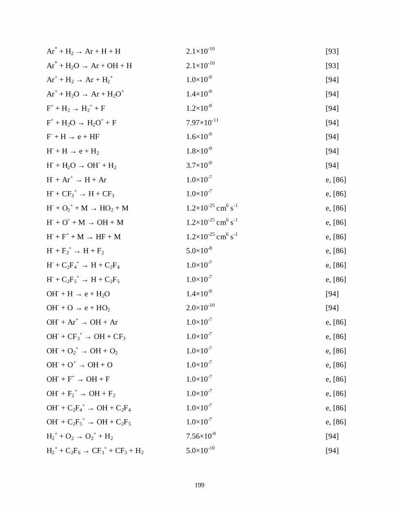
199
Ar* + H2 → Ar + H + H 2.1×10⁻¹⁰ [93]
Ar* + H2O → Ar + OH + H 2.1×10⁻¹⁰ [93]
Ar+ + H2 → Ar + H2+ 1.0×10⁻⁹ [94]
Ar+ + H2O → Ar + H2O+ 1.4×10⁻⁹ [94]
F+ + H2 → H2+ + F 1.2×10⁻⁹ [94]
F+ + H2O → H2O+ + F 7.97×10⁻¹¹ [94]
F- + H → e + HF 1.6×10⁻⁹ [94]
H- + H → e + H2 1.8×10⁻⁹ [94]
H- + H2O → OH- + H2 3.7×10⁻⁹ [94]
H- + Ar+ → H + Ar 1.0×10⁻⁷ e, [86]
H- + CF3+ → H + CF3 1.0×10⁻⁷ e, [86]
H- + O2+ + M → HO2 + M 1.2×10⁻²⁵ cm6 s-1 e, [86]
H- + O+ + M → OH + M 1.2×10⁻²⁵ cm6 s-1 e, [86]
H- + F+ + M → HF + M 1.2×10⁻²⁵ cm6 s-1 e, [86]
H- + F2+ → H + F2 5.0×10⁻⁸ e, [86]
H- + C2F4+ → H + C2F4 1.0×10⁻⁷ e, [86]
H- + C2F5+ → H + C2F5 1.0×10⁻⁷ e, [86]
OH- + H → e + H2O 1.4×10⁻⁹ [94]
OH- + O → e + HO2 2.0×10⁻¹⁰ [94]
OH- + Ar+ → OH + Ar 1.0×10⁻⁷ e, [86]
OH- + CF3+ → OH + CF3 1.0×10⁻⁷ e, [86]
OH- + O2+ → OH + O2 1.0×10⁻⁷ e, [86]
OH- + O+ → OH + O 1.0×10⁻⁷ e, [86]
OH- + F+ → OH + F 1.0×10⁻⁷ e, [86]
OH- + F2+ → OH + F2 1.0×10⁻⁷ e, [86]
OH- + C2F4+ → OH + C2F4 1.0×10⁻⁷ e, [86]
OH- + C2F5+ → OH + C2F5 1.0×10⁻⁷ e, [86]
H2+ + O2 → O2
+ + H2 7.56×10⁻⁹ [94]
H2+ + C2F6 → CF3
+ + CF3 + H2 5.0×10⁻¹⁰ [94]
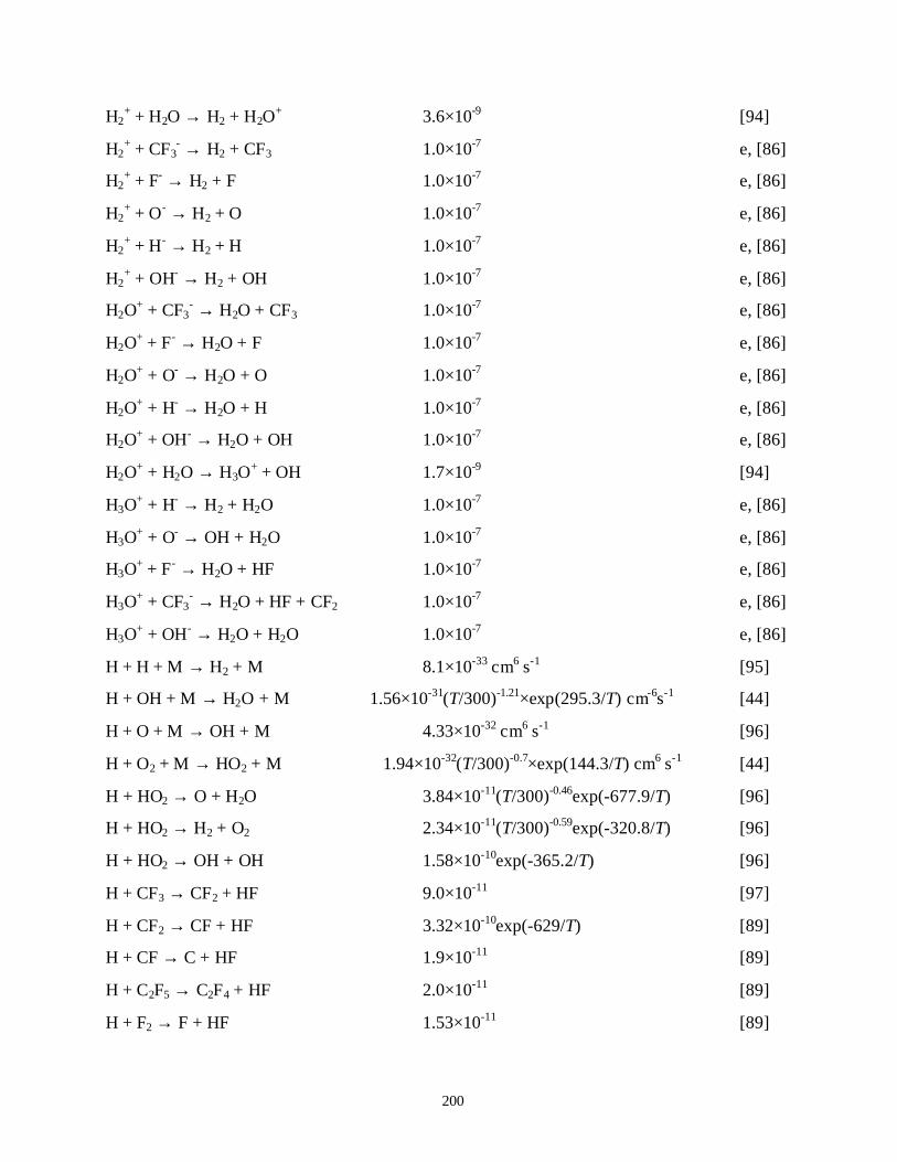
200
H2+ + H2O → H2 + H2O
+ 3.6×10⁻⁹ [94]
H2+ + CF3
- → H2 + CF3 1.0×10⁻⁷ e, [86]
H2+ + F- → H2 + F 1.0×10⁻⁷ e, [86]
H2+ + O- → H2 + O 1.0×10⁻⁷ e, [86]
H2+ + H- → H2 + H 1.0×10⁻⁷ e, [86]
H2+ + OH- → H2 + OH 1.0×10⁻⁷ e, [86]
H2O+ + CF3
- → H2O + CF3 1.0×10⁻⁷ e, [86]
H2O+ + F- → H2O + F 1.0×10⁻⁷ e, [86]
H2O+ + O- → H2O + O 1.0×10⁻⁷ e, [86]
H2O+ + H- → H2O + H 1.0×10⁻⁷ e, [86]
H2O+ + OH- → H2O + OH 1.0×10⁻⁷ e, [86]
H2O+ + H2O → H3O
+ + OH 1.7×10⁻⁹ [94]
H3O+ + H- → H2 + H2O 1.0×10⁻⁷ e, [86]
H3O+ + O- → OH + H2O 1.0×10⁻⁷ e, [86]
H3O+ + F- → H2O + HF 1.0×10⁻⁷ e, [86]
H3O+ + CF3
- → H2O + HF + CF2 1.0×10⁻⁷ e, [86]
H3O+ + OH- → H2O + H2O 1.0×10⁻⁷ e, [86]
H + H + M → H2 + M 8.1×10⁻³³ cm6 s-1 [95]
H + OH + M → H2O + M 1.56×10⁻³¹(T/300)-1.21×exp(295.3/T) cm-6s-1 [44]
H + O + M → OH + M 4.33×10⁻³² cm6 s-1 [96]
H + O2 + M → HO2 + M 1.94×10⁻³²(T/300)-0.7×exp(144.3/T) cm6 s-1 [44]
H + HO2 → O + H2O 3.84×10⁻¹¹(T/300)-0.46exp(-677.9/T) [96]
H + HO2 → H2 + O2 2.34×10⁻¹¹(T/300)-0.59exp(-320.8/T) [96]
H + HO2 → OH + OH 1.58×10⁻¹⁰exp(-365.2/T) [96]
H + CF3 → CF2 + HF 9.0×10⁻¹¹ [97]
H + CF2 → CF + HF 3.32×10⁻¹⁰exp(-629/T) [89]
H + CF → C + HF 1.9×10⁻¹¹ [89]
H + C2F5 → C2F4 + HF 2.0×10⁻¹¹ [89]
H + F2 → F + HF 1.53×10⁻¹¹ [89]
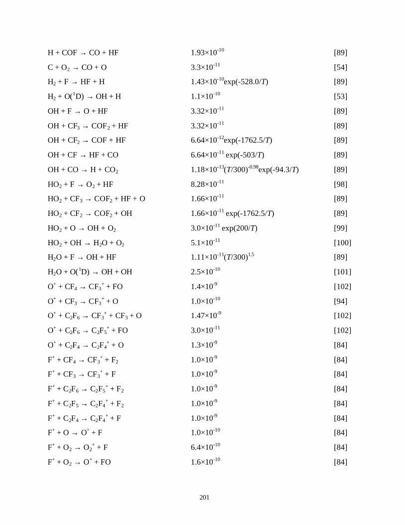
201
H + COF → CO + HF 1.93×10⁻¹⁰ [89]
C + O2 → CO + O 3.3×10⁻¹¹ [54]
H2 + F → HF + H 1.43×10⁻¹⁰exp(-528.0/T) [89]
H2 + O(1D) → OH + H 1.1×10⁻¹⁰ [53]
OH + F → O + HF 3.32×10⁻¹¹ [89]
OH + CF3 → COF2 + HF 3.32×10⁻¹¹ [89]
OH + CF2 → COF + HF 6.64×10⁻¹²exp(-1762.5/T) [89]
OH + CF → HF + CO 6.64×10⁻¹¹ exp(-503/T) [89]
OH + CO → H + CO2 1.18×10⁻¹³(T/300)-0.98exp(-94.3/T) [89]
HO2 + F → O2 + HF 8.28×10⁻¹¹ [98]
HO2 + CF3 → COF2 + HF + O 1.66×10⁻¹¹ [89]
HO2 + CF2 → COF2 + OH 1.66×10⁻¹¹ exp(-1762.5/T) [89]
HO2 + O → OH + O2 3.0×10⁻¹¹ exp(200/T) [99]
HO2 + OH → H2O + O2 5.1×10⁻¹¹ [100]
H2O + F → OH + HF 1.11×10⁻¹¹(T/300)1.5 [89]
H2O + O(1D) → OH + OH 2.5×10⁻¹⁰ [101]
O+ + CF4 → CF3+ + FO 1.4×10⁻⁹ [102]
O+ + CF3 → CF3+ + O 1.0×10⁻¹⁰ [94]
O+ + C2F6 → CF3+ + CF3 + O 1.47×10⁻⁹ [102]
O+ + C2F6 → C2F5+ + FO 3.0×10⁻¹¹ [102]
O+ + C2F4 → C2F4+ + O 1.3×10⁻⁹ [84]
F+ + CF4 → CF3+ + F2 1.0×10⁻⁹ [84]
F+ + CF3 → CF3+ + F 1.0×10⁻⁹ [84]
F+ + C2F6 → C2F5+ + F2 1.0×10⁻⁹ [84]
F+ + C2F5 → C2F4+ + F2 1.0×10⁻⁹ [84]
F+ + C2F4 → C2F4+ + F 1.0×10⁻⁹ [84]
F+ + O → O+ + F 1.0×10⁻¹⁰ [84]
F+ + O2 → O2+ + F 6.4×10⁻¹⁰ [84]
F+ + O2 → O+ + FO 1.6×10⁻¹⁰ [84]
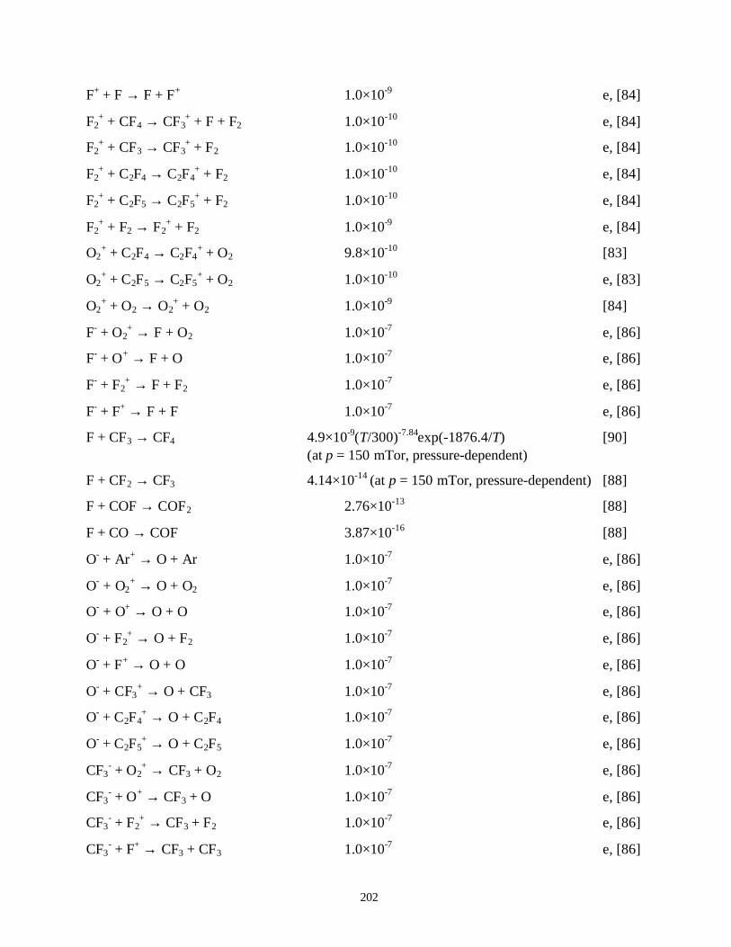
202
F+ + F → F + F+ 1.0×10⁻⁹ e, [84]
F2+ + CF4 → CF3
+ + F + F2 1.0×10⁻¹⁰ e, [84]
F2+ + CF3 → CF3
+ + F2 1.0×10⁻¹⁰ e, [84]
F2+ + C2F4 → C2F4
+ + F2 1.0×10⁻¹⁰ e, [84]
F2+ + C2F5 → C2F5
+ + F2 1.0×10⁻¹⁰ e, [84]
F2+ + F2 → F2
+ + F2 1.0×10⁻⁹ e, [84]
O2+ + C2F4 → C2F4
+ + O2 9.8×10⁻¹⁰ [83]
O2+ + C2F5 → C2F5
+ + O2 1.0×10⁻¹⁰ e, [83]
O2+ + O2 → O2
+ + O2 1.0×10⁻⁹ [84]
F- + O2+ → F + O2 1.0×10⁻⁷ e, [86]
F- + O+ → F + O 1.0×10⁻⁷ e, [86]
F- + F2+ → F + F2 1.0×10⁻⁷ e, [86]
F- + F+ → F + F 1.0×10⁻⁷ e, [86]
F + CF3 → CF4 4.9×10⁻⁹(T/300)-7.84exp(-1876.4/T) [90](at p = 150 mTor, pressure-dependent)
F + CF2 → CF3 4.14×10⁻¹⁴ (at p = 150 mTor, pressure-dependent) [88]
F + COF → COF2 2.76×10⁻¹³ [88]
F + CO → COF 3.87×10⁻¹⁶ [88]
O- + Ar+ → O + Ar 1.0×10⁻⁷ e, [86]
O- + O2+ → O + O2 1.0×10⁻⁷ e, [86]
O- + O+ → O + O 1.0×10⁻⁷ e, [86]
O- + F2+ → O + F2 1.0×10⁻⁷ e, [86]
O- + F+ → O + O 1.0×10⁻⁷ e, [86]
O- + CF3+ → O + CF3 1.0×10⁻⁷ e, [86]
O- + C2F4+ → O + C2F4 1.0×10⁻⁷ e, [86]
O- + C2F5+ → O + C2F5 1.0×10⁻⁷ e, [86]
CF3- + O2
+ → CF3 + O2 1.0×10⁻⁷ e, [86]
CF3- + O+ → CF3 + O 1.0×10⁻⁷ e, [86]
CF3- + F2
+ → CF3 + F2 1.0×10⁻⁷ e, [86]
CF3- + F+ → CF3 + CF3 1.0×10⁻⁷ e, [86]
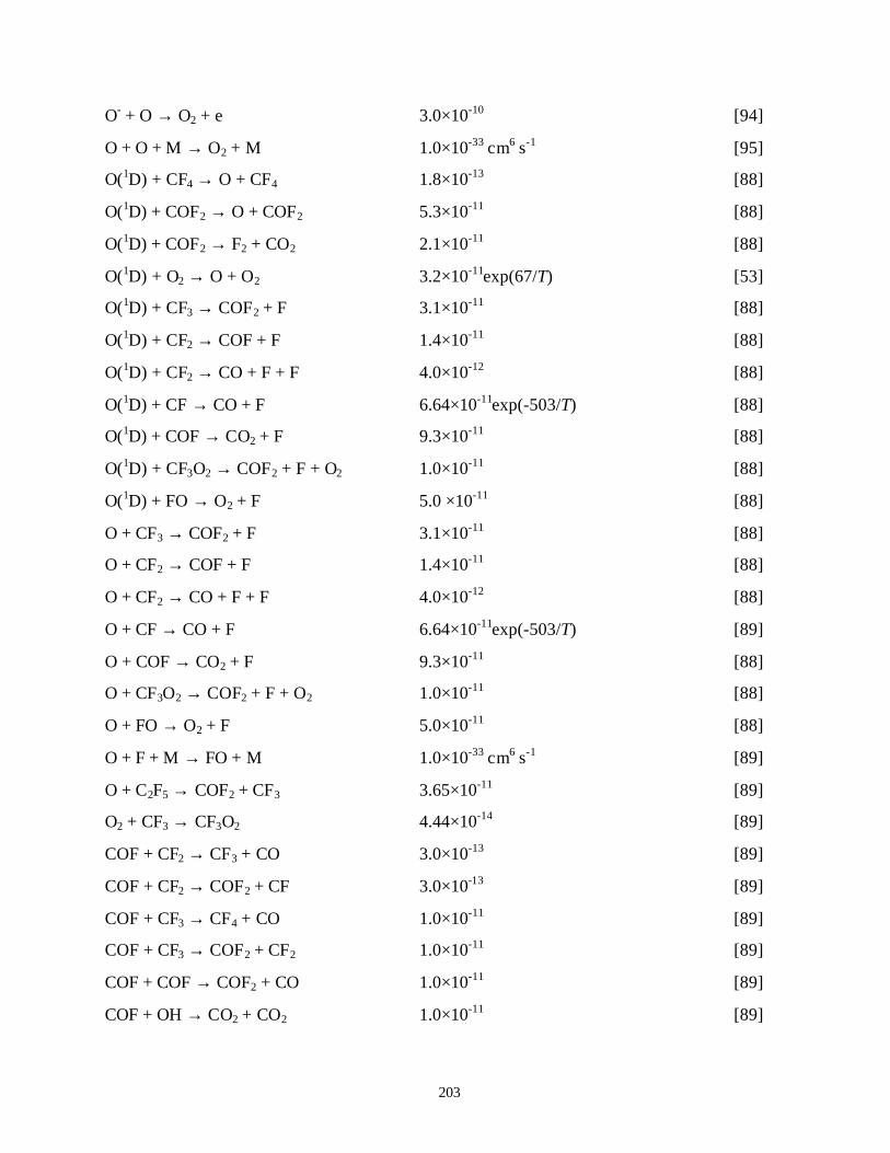
203
O- + O → O2 + e 3.0×10⁻¹⁰ [94]
O + O + M → O2 + M 1.0×10⁻³³ cm6 s-1 [95]
O(1D) + CF4 → O + CF4 1.8×10⁻¹³ [88]
O(1D) + COF2 → O + COF2 5.3×10⁻¹¹ [88]
O(1D) + COF2 → F2 + CO2 2.1×10⁻¹¹ [88]
O(1D) + O2 → O + O2 3.2×10⁻¹¹exp(67/T) [53]
O(1D) + CF3 → COF2 + F 3.1×10⁻¹¹ [88]
O(1D) + CF2 → COF + F 1.4×10⁻¹¹ [88]
O(1D) + CF2 → CO + F + F 4.0×10⁻¹² [88]
O(1D) + CF → CO + F 6.64×10⁻¹¹exp(-503/T) [88]
O(1D) + COF → CO2 + F 9.3×10⁻¹¹ [88]
O(1D) + CF3O2 → COF2 + F + O2 1.0×10⁻¹¹ [88]
O(1D) + FO → O2 + F 5.0 ×10⁻¹¹ [88]
O + CF3 → COF2 + F 3.1×10⁻¹¹ [88]
O + CF2 → COF + F 1.4×10⁻¹¹ [88]
O + CF2 → CO + F + F 4.0×10⁻¹² [88]
O + CF → CO + F 6.64×10⁻¹¹exp(-503/T) [89]
O + COF → CO2 + F 9.3×10⁻¹¹ [88]
O + CF3O2 → COF2 + F + O2 1.0×10⁻¹¹ [88]
O + FO → O2 + F 5.0×10⁻¹¹ [88]
O + F + M → FO + M 1.0×10⁻³³ cm6 s-1 [89]
O + C2F5 → COF2 + CF3 3.65×10⁻¹¹ [89]
O2 + CF3 → CF3O2 4.44×10⁻¹⁴ [89]
COF + CF2 → CF3 + CO 3.0×10⁻¹³ [89]
COF + CF2 → COF2 + CF 3.0×10⁻¹³ [89]
COF + CF3 → CF4 + CO 1.0×10⁻¹¹ [89]
COF + CF3 → COF2 + CF2 1.0×10⁻¹¹ [89]
COF + COF → COF2 + CO 1.0×10⁻¹¹ [89]
COF + OH → CO2 + CO2 1.0×10⁻¹¹ [89]
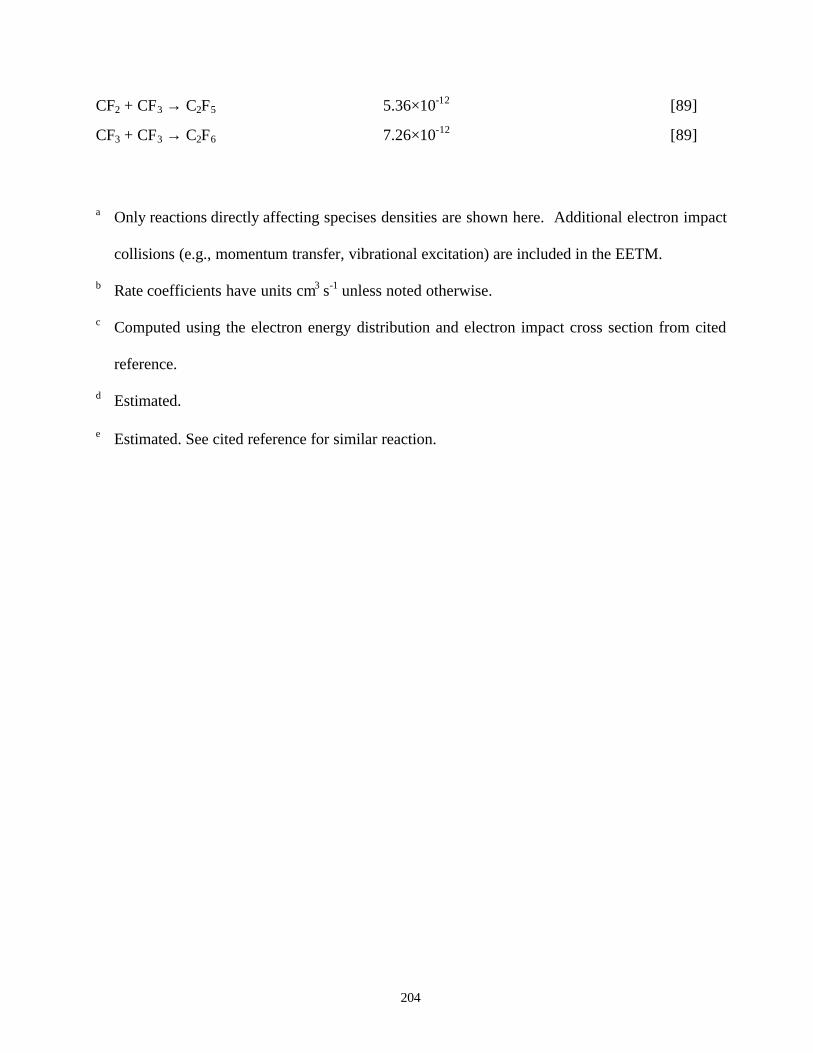
204
CF2 + CF3 → C2F5 5.36×10⁻¹² [89]
CF3 + CF3 → C2F6 7.26×10⁻¹² [89]
a Only reactions directly affecting specises densities are shown here. Additional electron impact
collisions (e.g., momentum transfer, vibrational excitation) are included in the EETM.
b Rate coefficients have units cm3 s-1 unless noted otherwise.
c Computed using the electron energy distribution and electron impact cross section from cited
reference.
d Estimated.
e Estimated. See cited reference for similar reaction.
205
B.1 References
[1] Y. Itikawa, M. Hayashi, A. Ichimura, K. Onda, K. Sakimoto, K. Takayanagi, M.
Nakamura, H. Nishimura, and T. Takayanagi, J. Phys. Chem. Ref. Data Reprint
Number 299, 15 (3), 985 (1986).
[2] J. M. A. Mitchell, Phys. Rep. 186, 215 (1990).
[3] R. R. Laher and F. R. Gilmore, J. Phys. Chem. Ref. Data 19, 277 (1990).
[4] A. V. Phelps, JILA Information Center Report No. 28, University of Colorado
(1985).
[5] E. Krishnakumar and S. K. Srivastava, Int. J. Mass Spect. Ion Proc. 113, 1 (1992).
[6] J. J. Lowke, and R. Morrow, IEEE Trans. Plasma Sci. 23, 661 (1995).
[7] J. B. A. Mitchell, Phys. Rep. 186, 215 (1990).
[8] M. Hayashi, J. De Physique, Colloque C7, Supplement 40, C7/45 (1979).
[9] M. Hayashi, Electron Collision Cross-Sections for Molecules Determined from
Beam and Swarm Data, edited by L.C. Pitchford, B.V. Mckoy, A. Chutjian, S.
Trajmar (Springer-Verlag, New York, 1989), pp. 234.
[10] M. Hayashi, in Proceedings of the Meeting of the 4th International Swarm
Seminar and the Inelastic Electron-Molecular Collision Symposium, July 19-23,
(1985), pp. 345.
[11] B. R. Rowe, F. Vallee, J. L. Queffelec, J. C. Gomet, and M. Morlais, J. Phys.
Chem. 88, 845 (1988).
[12] J.J. Lowke, A.V. Phelps and B.W. Irwin, J. Appl. Phys. 44, 4664 (1973).
[13] D. C. Griffin, M. S. Pindzola, T. W. Gorczyca, and N. R. Badnell, Phys. Rev. A
51, 2265 (1995).
206
[14] G. L. Rogoff, J. M. Kramer, and R. B. Piejek, Trans. Plasma Sci. 14, 103 (1986).
[15] K. Leiter, K. Stephan, E. Märk, and T. D. Märk, Plasma Chem. Plasma Proc. 4
(4), 235 (1984).
[16] J. B. A. Mitchell, Phys. Rpts. 186, 215 (1990)
[17] R. A. Bonham, Jpn. J. Appl. Phys., Part 1 33, 4157 (1994)
[18] M. Hayashi, in Gaseous Dielectrics V, edited by L. G. Christophorou and D. W.
Bouldin (Pergamon, New York, 1987), p. 456.
[19] W. L. Morgan, KINEMA: The Plasma Chemistry Code, Version 1.51,
(Monument, CO, 1994).
[20] M. Hayashi and T. Nimura, J. Appl. Phys. 54, 4879 (1983).
[21] K. Tachibana, Phys. Rev. A34, 1007 (1986).
[22] D. Rapp and P. Englander-Golden, J. Chem. Phys. 43, 1464 (1965).
[23] M. Hayashi, Nagoya Institute of Technology Report No. IPPJ-AM-19, 1991.
[24] F. Kannari, M. Obara, T. Fujioka, J. Appl. Phys. 57, 4390 (1985)
[25] N. J. Mason and W. R. Newell, J. Phys. B 20, 1357 (1987)
[26] T. Y. Suzuki, Y. Sakai, B. S. Min, T. Takayanagi, K. Wakiya, H. Suzuki, T.
Inaba, and H. Takuma, Phys. Rev. A 43, 5867 (1991).
[27] D. Rapp and P. Englander-Golden, J. Chem. Phys. 43, 1464 (1965).
[28] D. J. Eckstrom, H. H. Nakano, D. C. Lorents, T. Rothem, J. A. Betts, M. E.
Lainhart, D. A. Dakin, and J. A. Maenchen, J. Appl. Phys. 64, 1679 (1988).
[29] J. W. Shon, Ph.D. dissertation, University of Illinois, 1993.
[30] J. Bretagne, J. Godart, and V. Puech, J. Phys. D 15, 2205 (1982).
[31] R. A. Bonham, Jpn. J. Appl. Phys., Part 1 33, 4157 (1994)
207
[32] M. Hayashi, in Gaseous Dielectrics V, edited by L. G. Christophorou and D. W.
Bouldin (Pergamon, New York, 1987), p. 456.
[33] M. Hayashi and T. Nimura, J. Appl. Phys. 54, 4879 (1983).
[34] J. C. Person and D. O. Ham, Radiat. Phys. Chem. 31, 1 (1988).
[35] J. P. Boeuf and E. E. Kunhardt, J. Appl. Phys. 60, 915, (1986).
[36] L. G. Piper, J. Chem. Phys. 87, 1625 (1987).
[37] F. Westley, J. T. Herron, R. J. Cvetanovic, R. F. Hampson, and W. G. Mallard,
NIST Chemical Kinetics Database, NIST Standard Reference Database 17,
National Institute of Standards and Technology, Standard Reference Data
Program, Gaithersburg, MD 20899.
[38] L. Elias, E. A. Ogryzlo, and H. I. Schiff, Can. J. Chem. 37, 1680 (1959).
[39] W. Tsang and R. F. Hampson, J. Phys. Chem. Ref. Data, 15, 1087 (1986).
[40] R. Atkinson, D. L. Baulch R. A. Cox, R. F. Hampson, Jr., J. A. Kerr, and J. Troe,
J. Phys. Chem. Ref. Data, 18, 881 (1989).
[41] W. G. Mallard, F. Westley, J. T. Herron, and R. F. Hampson, NIST Chemical
Kinetics Database-Version 6.0, NIST Standard Reference Database 17. National
Institute of Standards and Technology, NIST Standard Reference Data,
Gaithersburg, MD (1994).
[42] R. K. Bera and R. J. Hanrahan, J. Appl. Phys. 62, 2523 (1987).
[43] D. C. Robie, S. Arepalli, N. Presser, T. Kitsopoulos, and R. J. Gordon, J. Chem.
Phys. 92, 7382 (1990).
208
[44] D. L. Baulch, C. J. Cobos, R. A. Cox, C. Esser, P. Frank, T. Just, J. A. Kerr, M. J.
Pilling, J. Troe, R. W. Walker and J. Warnatz, J. Phys. Chem. Ref. Data 21, 411
(1992).
[45] S. Mukkavilli, C. K. Lee, K. Varghese, and L. L. Tavlarides, IEEE Trans. Plasma
Sci. 16, 652 (1988).
[46] K. V. Baiadze, V. M. Vetsko, S. A. Zdhanok, A. P. Napartovich, and A. N.
Starotin, Sov. J. Plasma Phys. 5, 515 (1979).
[47] W. Tsang and R. F. Hampson, J. Phys. Chem. Ref. Data 15, 1087 (1986).
[48] R. Atkinson, D. L. Baulch R. A. Cox, R. F. Hampson, Jr., J. A. Kerr, and J. Troe,
J. Phys. Chem, Ref. Data, 18, 881 (1989).
[49] R. E. Olson, J. R. Peterson, and J. Moseley, J. Chem. Phys. 53, 3391 (1970).
[50] G. Dixon-Lewis, Proc. Roy. Soc. London A 330, 219 (1972).
[51] W. D. Chang and S. M. Senkan, Environ. Sci. Technol. 23, 442 (1989).
[52] W. D. Chang, S. B. Karra, and S. M. Senkan, Combust. Sci. Technol. 49, 107
(1986).
[53] R. Atkinson, D. L. Baulch, R. A. Cox, R. F. Hampson, J. A. Kerr, and J. Troe, J.
Phys. Chem. Ref. Data 21,1125 (1992).
[54] D. Husain, and L. J. Kirsch, Trans. Faraday Soc. 67, 2025 (1971).
[55] R. T. Watson, J. Phys. Chem. Ref. Data 6, 871 (1977).
[56] Z. Falkenstein, J. Adv. Oxid. Technol. 1, 223 (1997).
[57] W. Forst and F. Caralp, J. Chem. Soc. Faraday Trans. 87, 2307 (1991).
[58] M. Weissman, and S. W. Benson, Int. J. Chem. Kinet. 12, 403 (1980).
[59] C. J. Cobos and J Troe, Chem. Phys. Lett. 113, 419 (1985).
209
[60] J. T. Herron, J. Phys. Chem. Ref. Data 17, 967 (1988).
[61] J. J. Russell, J. A. Seetula, D. Gutman, F. Danis, F. Caralp, P. D. Lightfoot, R.
Lesclaux, C. F. Melius and S. M. Senkan, J. Phys. Chem. 94, 3277 (1990).
[62] P. S. Stevens; J. G. Anderson, J. Phys. Chem. 96, 1708 (1992).
[63] P. H. Wine, J. M. Nicovich, and A. R. Ravishankara, J. Phys. Chem. 89, 3914
(1985).
[64] R. B. Boodaghians, I. W. Hall, and R. P. Wayne, J. Chem. Soc. Faraday Trans.
83, 529 (1987).
[65] J. Shi and J. R. Barker, Int. J. Chem. Kinet. 22, 1283 (1990).
[66] J. M. Nicovich, K. D. Kreutter, and P. H. Wine, J. Chem. Phys. 92, 3539 (1990).
[67] J. T. Herron and R. E. Huie, J. Phys. Chem. Ref. Data 2, 467 (1973).
[68] D. Albritton, At. Data. Nucl. Data Tables 22, 8 (1978).
[69] L. G. Piper, J. E. Velazco, and D. W. Setser, J. Chem. Phys. 59, 3323 (1973).
[70] D. L. Baulch, J. Duxbury, S. J. Grant, and D. C. Montague, J. Phys. Chem. Ref.
Data 10, Suppl. 1, 1 (1981).
[71] F. Kannari, D. Kimura and J. J. Ewing, J. Appl. Phys. 68, 2615 (1990).
[72] T. H. Johnson, H. E. Cartland, T. C. Genoni, and A. M. Hunter, J. Appl. Phys. 66,
5707 (1988).
[73] H. Hokazono, K. Midoridawa, M. Obara, and T. Fujioda, J. Appl. Phys. 56, 680
(1984).
[74] M. Ohwa, T. J. Moratz, and M. J. Kushner, J. Appl. Phys. 66, 5131 (1989).
[75] N. Nishida, T. Takashima, F. K. Tittel, F. Kannari and M. Obara, J. Appl. Phys.
67, 3932 (1990).
210
[76] D. C. Lorents, 37th Gaseous Electronics Conference, Boulder, CO, 1984 (Bull.
Amer. Phy. Soc. 30, 148 (1985).
[77] J. M. Hoffman and H. B. Moreno, SAND80-1486, UC-34a (1980).
[78] L. A. Levin, S. E. Moody, E. L. Klosterman, R. E. Center, and J. J. Ewing, IEEE
J. Quantum Electron. 17, 2282 (1981).
[79] D. L. Huestis, R. M. Hill, H. H. Nakano, and D. C. Lorents, J. Chem. Phys. 69,
5133 (1978).
[80] M. M. Turner and W. Smith, IEEE Trans. Plasma Sci. 19, 350 (1990).
[81] O. Lamrous, A. Gaouar, and M. Yousfi, J. Appl. Phys., 79, 6775 (1996).
[82] E. Fisher, M. E. Weber, and P. B. Armentrout, J. Chem. Phys. 76, 4932 (1982).
[83] G. K. Jarvis, C. A. Mayhew, and R. P. Tuckett, J. Phys. Chem. 100, 17166
(1996).
[84] P. K. Leichner and R. J. Ericson, Phys. Rev. A 9, 251 (1974).
[85] J. E. Velazco, J. H. Koltz, and D. W. Sester, J. Chem. Phys. 65, 3468 (1976).
[86] R. E. Olson, J. R. Peterson, and J. Moseley, J. Chem. Phys. 53, 3391 (1971).
[87] E. L. Duman, N. P. Tishchenko, and I. P. Shmatov, Dokl. Phys. Chem. 295, 5
(1987).
[88] I. C. Plumb, K. R. Ryan, Plasma Chem. Plasma Proc. 6, 205 (1986).
[89] D. R. F. Burgess, Jr., M. R. Zachariah, W. Tsang, and P. R. Westmoreland, Prog.
Energy Combust. Sci. 21, 453,1996.
[90] D. R. F. Burgess, Jr., National Institute of Standards and Technology (private
communication).
211
[91] D. L. Parent, R. Derai, G. Mauclaire, M. Heninger, R. Marx, M. E. Rincon, A.
O’Keefe, and M. T. Bowers, Chem. Phys. Lett. 117, 127 (1985).
[92] P. Gaucherel, Int. J. Mol. Spec. 25, 211 (1977).
[93] L. G. Piper, J. E. Velazco, and D. W. Setser, J. Chem. Phys. 59, 4932 (1973).
[94] Y. Ikezoe, S. Matsuoka, M. Takebe, and A. Viggiano, Gas-phase Ion-Molecule
Reaction Rate Constants Through 1986 (Maruzen, Tokyo, 1987).
[95] J. C. Person and D. O. Ham, Radiat. Phys. Chem. 31, 1 (1988).
[96] W. Tsang and R. F Hampson, J. Phys. Chem. Ref. Data 15, 1087 (1986).
[97] C. Tsai and D. L. McFadden, J. Phys. Chem. 93, 2471 (1989).
[98] C. D. Walther and H. G. Wagner, Ber. Bunsenges. Phys. Chem. 87, 403 (1983).
[99] W. B DeMore, D. M. Golden, R. F. Hampson, C. J. Howard, M. J. Kurylo, M. J.
Molina, A. R. Ravishankara, and S. P. Sander, JPL Publication 1, 87 (1987).
[100] J. P. Burrows, D. I. Cliff, G. W. Harris, B. A. Thrush, and J. P. T. Wilkinson,
Proc. Roy. Soc. London A 368, 463 (1980).
[101] L. C. Lee, and T. G. Slanger, Geophys. Res. Lett. 6,165 (1979).
[102] E. R. Fisher and P. R. Armentrout, J. Phys. Chem. 95, 6118 (1991).
Recommended