HAL Id: hal-00322154https://hal.archives-ouvertes.fr/hal-00322154
Submitted on 16 Sep 2008
HAL is a multi-disciplinary open accessarchive for the deposit and dissemination of sci-entific research documents, whether they are pub-lished or not. The documents may come fromteaching and research institutions in France orabroad, or from public or private research centers.
L’archive ouverte pluridisciplinaire HAL, estdestinée au dépôt et à la diffusion de documentsscientifiques de niveau recherche, publiés ou non,émanant des établissements d’enseignement et derecherche français ou étrangers, des laboratoirespublics ou privés.
Dynamic viscosity estimation of hydrogen sulfide using apredictive scheme based on molecular dynamics.
Guillaume Galliéro, Christian Boned
To cite this version:Guillaume Galliéro, Christian Boned. Dynamic viscosity estimation of hydrogen sulfide using a predic-tive scheme based on molecular dynamics.. Fluid Phase Equilibria, Elsevier, 2008, 269 (1-2), pp.19-24.<10.1016/j.fluid.2008.04.017>. <hal-00322154>
1
Dynamic viscosity estimation of hydrogen sulfide using a predictive scheme
based on molecular dynamics.
Guillaume Galliero*, Christian Boned
Laboratoire des Fluides Complexes (UMR-5150), Université de Pau et des Pays de l’Adour, BP 1155, F-64013 PAU Cedex, France.
*Corresponding author, Email: [email protected]; Tel: +33 5 57 40 7704; Fax:
+33 5 57 40 7695.
Abstract
An approach based on molecular dynamics results on Lennard-Jones spheres is proposed to
model the viscosity of hydrogen sulfide, H2S. The molecular parameters, that have a strong
physical meaning, are the depth of the potential, and the length at which the potential is null
(the “molecular diameter”), which take into account the dipolar moment of the hydrogen
sulphide through an isotropic dipolar approximation. The interest of the method is that the
adjustment does not involve any viscosity data because only density values have been used in
order to estimate the molecular parameters. Consequently, the model is entirely predictive. A
comparison between the data generated by our model, REFPROP7 and REFPROP8 database
and the few available experimental viscosity data (dilute gas and saturated liquid) is
performed and clearly demonstrates the performance of this predictive model. It is even
shown that this model is, without fitting, slightly better than REFPROP7 and REFPROP8
which uses viscosity experimental database to adjust their parameters. In addition, in typical
petroleum reservoirs conditions, it is shown that non negligible deviations appear when
comparing results predicted by REFPROP7, REFPROP8 and the model proposed. Due to its
predictive nature, we believe that the values evaluated by the proposed model make sense in
such reservoir conditions, at least for industrial purposes. Moreover, the scheme proposed is

2
shown to be very easily extended to deal with mixtures involving H2S with the limit that the
Lennard-Jones fluid model is appropriate for the other species of the mixtures.
Keywords:
Hydrogen sulfide; Viscosity; Molecular Dynamics; Lennard-Jones; Acid gas.

3
1. Introduction
Acid gas mixtures (ie natural gases containing hydrogen sulfide H2S and/or carbon dioxide
CO2) are often encountered in the petroleum industry. For the systems containing hydrogen
sulfide, experiments on their thermophysical properties are very scarce because of the very
high toxicity of H2S which leads to very complicated safety procedures for the
experimentalists. This is especially true for the high pressures and temperatures conditions of
petroleum reservoir. As we recently emphasized [1], this lack of knowledge is particularly
apparent concerning transport properties. Concerning the dynamic viscosity, the available
experimental database is very small. The reader could find a presentation of the works
available in the literature in a recent work [2]. It is worth to mention the work of Liley et al.
[3], which proposes after critical analysis of the available data, a table with 18 values between
190 and 350 K for the saturated liquid (pressure up to 6 MPa) and 21 values for the dilute gas
as a function of temperature between 250 and 500 K. For the dilute gas these authors propose
an equation after the analysis of several experimental data sets. The analysis recently
presented in [2] confirms also the fact that the number of confident experimental viscosity
data is very small. In particular, it seems that the data set of Monteil et al. [4] at high pressures
and temperatures should be not considered [2] as these data exhibited inconsistencies with the
rest of the data set.
As experiments are difficult to perform on H2S, alternatives are highly encouraged. In [2] the
authors propose a hydrogen sulfide viscosity modeling based on the friction-model [5]. The
authors propose a correlation in order to evaluate the viscosity in larges pressure and
temperature range. They give a hydrogen sulfide reference friction theory model, which
involve 18 adjustable parameters (and 4 more parameters for the dilute gas). But as the
number of experimental data is too low for their fitting procedure, they have to make some
assumptions on the H2S viscosity behavior. They acknowledge that their model is sensitive
4
and requires a good database to be regressed against for optimal performance. Therefore, in
order to develop a reasonable model to be used as a reference H2S model, the available data
has been complemented with scaled data from fluids that may show a similar qualitative
behaviour as H2S, based on supposed similarities between hydrogen sulfide and carbon
dioxide or ethane. They indicate that their H2S model has been developed by combining the
few available reliable H2S data with low pressure scaled CO2 data and elevated pressure
scaled C2H6 data. Then, they adjusted the 18+4 parameters (parameters without physical
meaning). Next to that, the general reference friction-theory model is used as a reference for
the tuning of so called one-parameter viscosity model. It should not be forgotten that in fact
this modeling is made with a database not only based on experimental data, but also on scaled
CO2 and C2H6 viscosities (without any explanation about the scaling nor the number of data
evaluated in such way). Nevertheless, due to the lack of information on the dynamic viscosity
of H2S, this model has been implemented in the software REFPROP 8 [6] developed by the
National Institute of Standards and Technology (NIST), because a better model is lacking.
In order to avoid to make speculative assumptions on the values of the viscosity of the H2S,
we propose in this paper another approach, based on molecular dynamics results for Lennard-
Jones spheres, in which only 2 adjusted molecular parameters with physical meaning are used,
only adjusted to density data [1]. These parameters are ε, the strength of the potential, and
σ the length at which the potential is zero (the “molecular diameter”), which take into account
the dipolar moment of the hydrogen sulphide through an isotropic dipolar approximation [7].
The adjustment does not involve any viscosity data and consequently the model is entirely
predictive. As no adjustment has been done to viscosity data, the comparison between the data
generated by our model and the few available viscosity data is significant for the performance
and of the physical meaning of the model, and we can therefore expect that the values
evaluated at pressures and temperatures outside the pressure and temperature range of the

5
available data could be considered significant, at least for industrial purposes, particularly in
dense states at high pressure and high temperature, as in reservoir conditions. Finally, it is
mentioned here that, in a previous study [1], we already have given some molecular dynamic
results for the viscosity of H2S, but we did not develop in this previous work a model which is
easy to implement in computing software.
2. Modeling
2.1. Interaction potential
In this work, it is assumed that the H2S molecule can be correctly described by a one center
spherical particle (united atom). In addition, to describe intermolecular interactions occurring
between two particles, it is assumed that the total interaction potential can be simply described
by the sum of a non polar contribution and a contribution due to the dipolar moment of the
hydrogen sulfide:
polarpolarnonTot UUU += − (1)
To describe the non polar interactions, the usual Lennard-Jones 12-6 (LJ) effective potential is
used:
−
=−
612
4rr
U polarnon
σσε (2)
where ε is the potential strength, σ the length at which the potential is zero (the “molecular
diameter”) and r the intermolecular separation.
The dipolar contribution, it is modelled by a Keesom potential [8], which writes for pure H2S:
6
4
3
1
rTkU
B
polar
µ−= (3)
where µ is the dipole moment, kB the Boltzmann constant and T the temperature.
6
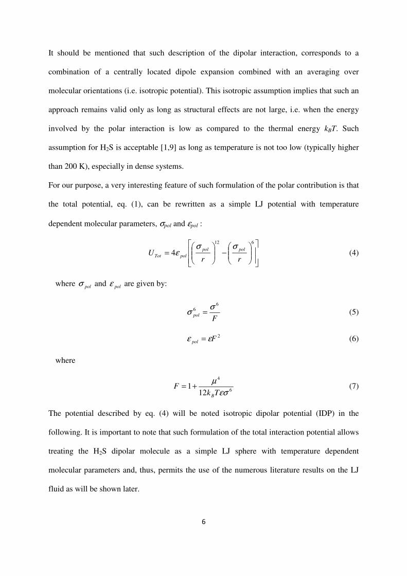
It should be mentioned that such description of the dipolar interaction, corresponds to a
combination of a centrally located dipole expansion combined with an averaging over
molecular orientations (i.e. isotropic potential). This isotropic assumption implies that such an
approach remains valid only as long as structural effects are not large, i.e. when the energy
involved by the polar interaction is low as compared to the thermal energy kBT. Such
assumption for H2S is acceptable [1,9] as long as temperature is not too low (typically higher
than 200 K), especially in dense systems.
For our purpose, a very interesting feature of such formulation of the polar contribution is that
the total potential, eq. (1), can be rewritten as a simple LJ potential with temperature
dependent molecular parameters, σpol and εpol :
−
=
612
4rr
Upolpol
polTot
σσε (4)
where polσ and polε are given by:
F
pol
66 σ
σ = (5)
2Fpol εε = (6)
where
6
4
121
εσ
µ
TkF
B
+= (7)
The potential described by eq. (4) will be noted isotropic dipolar potential (IDP) in the
following. It is important to note that such formulation of the total interaction potential allows
treating the H2S dipolar molecule as a simple LJ sphere with temperature dependent
molecular parameters and, thus, permits the use of the numerous literature results on the LJ
fluid as will be shown later.

7
2.2. H2S molecular parameters
The adjustment of two molecular parameters, ε and σ, of the H2S molecule has been done in a
previous work [1]. The following procedure was applied [1]: using for the dipole moment of
the H2S, the commonly accepted literature value µ=0.9D [10], three different state points have
been considered, one on the liquid saturation curve (T=273 K, P=1.028 MPa), and two at high
temperature/high pressures (T=498.2 K and P=10.02 or 39.993 MPa) for which experimental
density results exist [11,12]. Then, for these three state points, using constant pressure
molecular dynamics simulations (NPT), σ and ε have been obtained by fitting the
experimental densities. The molecular parameters obtained are summarized in Table 1. In
Table 1 the values of the dipole moment (taken from [10]) and of the molecular mass are also
given.
3. Results
3.1. H2S density
Among the various equations of state (EoS) that represent correctly the thermodynamic
behavior of the Lennard-Jones fluid, we have used the theoretically founded EoS of Kolafa
and Nezbeda [13], which is based on a perturbated virial expansion. In a previous work [1], it
has been shown that this EoS combined with the potential given by eq. (4) and the parameters
provided in Table I allows a reasonable estimation of the H2S density when T and P are fixed.
More precisely, this scheme yields an Average Absolute Deviation (AAD) for ρ equal to 0.51
% with a Maximum Deviation (MxD) of 0.97 % [1] when compared to the subcritical data of
Ihmels and Gmehling [12] containing 206 points (T=273-363 K, P=3-40 MPa). Recall here
that only 3 density data points have been used in order to adjust the 2 parameters ε and σ
8
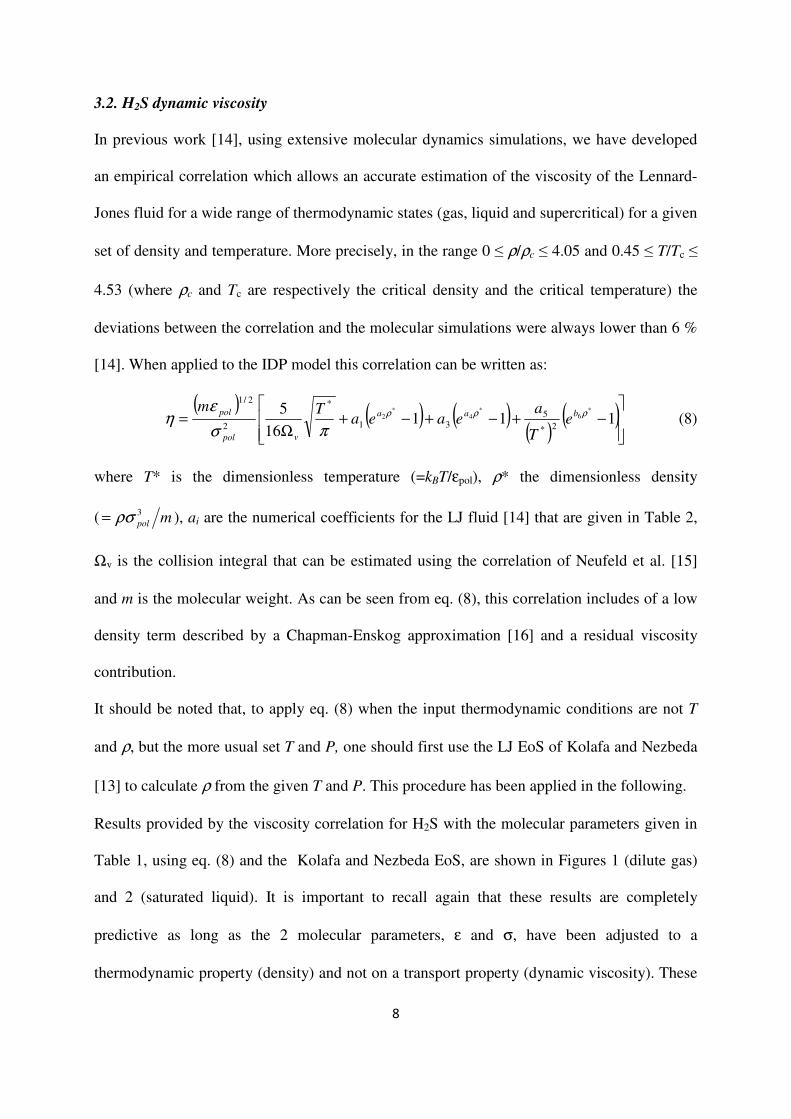
3.2. H2S dynamic viscosity
In previous work [14], using extensive molecular dynamics simulations, we have developed
an empirical correlation which allows an accurate estimation of the viscosity of the Lennard-
Jones fluid for a wide range of thermodynamic states (gas, liquid and supercritical) for a given
set of density and temperature. More precisely, in the range 0 ≤ ρ/ρc ≤ 4.05 and 0.45 ≤ T/Tc ≤
4.53 (where ρc and Tc are respectively the critical density and the critical temperature) the
deviations between the correlation and the molecular simulations were always lower than 6 %
[14]. When applied to the IDP model this correlation can be written as:
( ) ( ) ( )
( )( )
−+−+−+
Ω= 111
165 *
6*
4*
2
2*
531
*
2
2/1
ρρρ
πσ
εη baa
vpol
pole
T
aeaea
Tm (8)
where T* is the dimensionless temperature (=kBT/εpol), ρ* the dimensionless density
( mpol
3ρσ= ), ai are the numerical coefficients for the LJ fluid [14] that are given in Table 2,
Ωv is the collision integral that can be estimated using the correlation of Neufeld et al. [15]
and m is the molecular weight. As can be seen from eq. (8), this correlation includes of a low
density term described by a Chapman-Enskog approximation [16] and a residual viscosity
contribution.
It should be noted that, to apply eq. (8) when the input thermodynamic conditions are not T
and ρ, but the more usual set T and P, one should first use the LJ EoS of Kolafa and Nezbeda
[13] to calculate ρ from the given T and P. This procedure has been applied in the following.
Results provided by the viscosity correlation for H2S with the molecular parameters given in
Table 1, using eq. (8) and the Kolafa and Nezbeda EoS, are shown in Figures 1 (dilute gas)
and 2 (saturated liquid). It is important to recall again that these results are completely
predictive as long as the 2 molecular parameters, ε and σ, have been adjusted to a
thermodynamic property (density) and not on a transport property (dynamic viscosity). These
9
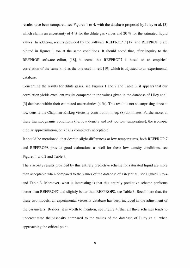
results have been compared, see Figures 1 to 4, with the database proposed by Liley et al. [3]
which claims an uncertainty of 4 % for the dilute gas values and 20 % for the saturated liquid
values. In addition, results provided by the software REFPROP 7 [17] and REFPROP 8 are
plotted in figures 1 to4 at the same conditions. It should noted that, after inquiry to the
REFPROP software editor, [18], it seems that REFPROP7 is based on an empirical
correlation of the same kind as the one used in ref. [19] which is adjusted to an experimental
database.
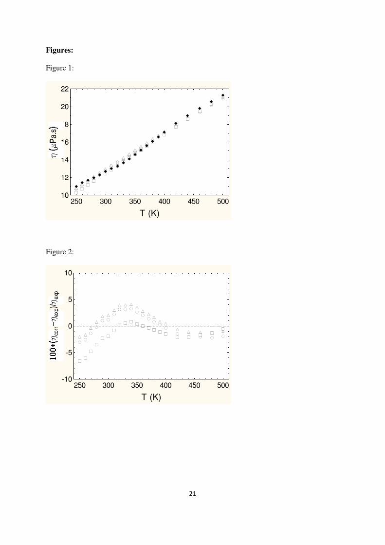
Concerning the results for dilute gases, see Figures 1 and 2 and Table 3, it appears that our
correlation yields excellent results compared to the values given in the database of Liley et al.
[3] database within their estimated uncertainties (4 %). This result is not so surprising since at
low density the Chapman-Enskog viscosity contribution in eq. (8) dominates. Furthermore, at
these thermodynamic conditions (i.e. low density and not too low temperature), the isotropic
dipolar approximation, eq. (3), is completely acceptable.
It should be mentioned, that despite slight differences at low temperatures, both REFPROP 7
and REFPROP8 provide good estimations as well for these low density conditions, see
Figures 1 and 2 and Table 3.
The viscosity results provided by this entirely predictive scheme for saturated liquid are more
than acceptable when compared to the values of the database of Liley et al., see Figures 3 to 4
and Table 3. Moreover, what is interesting is that this entirely predictive scheme performs
better than REFPROP7 and slightly better than REFPROP8, see Table 3. Recall here that, for
these two models, an experimental viscosity database has been included in the adjustment of
the parameters. Besides, it is worth to mention, see Figure 4, that all three schemes tends to
underestimate the viscosity compared to the values of the database of Liley et al. when
approaching the critical point.

10
In addition, the trends obtained by our new approach are really consistent, i.e. at low
temperature (below 270 K) the underestimation increases when temperature decreases, see
Figure 4, which is certainly due to the IDP limitations for such conditions. Besides, for the
saturated liquid, if the density deduced from REFPROP8 (which uses reference [20]) are used
instead of those deduced using the Kolafa-Nezbeda EOS, the viscosity correlation, eq. (8),
yields slightly better results with AAD=4.3 % and MxD=13.9 % instead of 5.5% and 15.6 %,
see Table 3.
The thermodynamic conditions of interest for the petroleum industry are in general between
273.15 and 423.15 K and between 10 and 140 MPa. Unfortunately, for such conditions only
the experimental data sets of Monteil et al. [4] are available, and it has been shown that these
values should be not considered [2] as these data exhibited inconsistencies. So, for pressures
from 10 to 140 MPa, with a step a 10 MPa, and temperatures from 273.15 to 423.15 K, with a
step of 50 K, REFPROP7, REFPROP8 and the new scheme have been used to estimate
viscosities, see Figure 5. As a preliminary test of the validity of the results provided by the
proposed scheme for such thermodynamic conditions, nonEquilibrium MD simulations have
been performed at T=273.15 K, P=10 MPa and T=423.15 K, P=140 MPa using the procedure
described in a previous work [1]. For these two dense states, we obtain by MD simulations
respectively η = 168±8 10-6 Pa.s and 143±6 10-6 Pa.s whereas the proposed scheme based on
eq. (8) yields 166 10-6 Pa.s and 144 10-6 Pa.s. Such good agreement is not surprising as long
as eq. (8) is able to represent MD results of LJ sphere [14] (with a MxD below 6 %) for a
wide range of thermodynamic conditions that encompass those studied in this work.
From the results provided in Figure 5, it appears that in all cases the values predicted by the
new scheme are between those predicted by REFPROP7 and REFPROP8, and generally
closer to those of REFPROP8. In addition, the larger the viscosity, the larger the deviations
between results from the different models (between REFPROP7 and REFPROP8 the

11
deviation reaches 34.6% at P=140 MPa and T=273.15 K). Compared to our scheme,
REFPROP7 yields an AAD=12.2 % with a MxD=18.5 % and REFPROP8 an AAD=4.4%
with a MxD=15.4 %.
It is important to note that, because the new scheme is completely predictive, and the IDP is
physically acceptable for not too low temperature, the results provided by this correlation for
the high pressures conditions tested here should be as good as those given at these conditions
in the database of Liley et al.. That is not necessary the case for the fitted approaches such as
those used in REFPROP7 and REFPROP8 as they have been adjusted to a rather limited
experimental database. Hence, the reliability of the predictions of such models outside the
range of the conditions of the experimental database is probably more questionable as shown
by the differences noted in Figure 5.
3.3. Extension to mixtures
One nice feature of the scheme proposed is that it can be very easily extended to deal with
mixtures involving H2S under the condition that the LJ fluid model is appropriate for the other
species of the mixtures. To do so, once the molecular parameters (mi, σii, εii) of each
compound i are known (plus the dipolar moment of H2S), one has to use the van der Waals
one fluid approximation [21] which consists in lumping the different compounds of the
mixture into one equivalent pseudocomponent using the molar fraction xi:
∑=i
iix mxm (10)
∑∑=i j
ijjix xx 33 σσ (11)
∑∑=i j
ijijjixx xx 33 σεσε (12)
The cross molecular parameters, εij and σij are defined by a set of combination rules which are
usually the Lorentz-Berthelot (LB) ones:
12
+=
2jjii
ij
σσσ (13)
( ) 21
jjiiij εεε = (14)
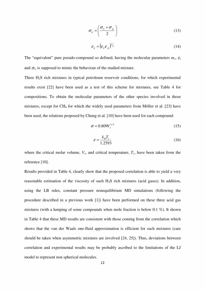
The “equivalent” pure pseudo-compound so defined, having the molecular parameters mx, εx
and σx, is supposed to mimic the behaviour of the studied mixture.
Three H2S rich mixtures in typical petroleum reservoir conditions, for which experimental
results exist [22] have been used as a test of this scheme for mixtures, see Table 4 for
compositions. To obtain the molecular parameters of the other species involved in those
mixtures, except for CH4 for which the widely used parameters from Möller et al. [23] have
been used, the relations proposed by Chung et al. [10] have been used for each compound:
3/1809.0 cV=σ (15)
2593.1
cBTk=ε (16)
where the critical molar volume, Vc, and critical temperature, Tc, have been taken from the
reference [10].
Results provided in Table 4, clearly show that the proposed correlation is able to yield a very
reasonable estimation of the viscosity of such H2S rich mixtures (acid gases). In addition,
using the LB rules, constant pressure nonequilibrium MD simulations (following the
procedure described in a previous work [1]) have been performed on these three acid gas
mixtures (with a lumping of some compounds when mole fraction is below 0.1 %). It shown
in Table 4 that these MD results are consistent with those coming from the correlation which
shows that the van der Waals one-fluid approximation is efficient for such mixtures (care
should be taken when asymmetric mixtures are involved [24, 25]). Thus, deviations between
correlation and experimental results may be probably ascribed to the limitations of the LJ
model to represent non spherical molecules.

13
4. Conclusion
The approach proposed in this paper to estimate hydrogen sulfide viscosity is based on
molecular dynamics results, with only 2 adjusted molecular parameters with physical
meaning, adjusted to experimental density data. These parameters are ε, the strength of the
Lennard-Jones potential, and σ the length at which the potential is zero, the “molecular
diameter”, which take into account the dipolar moment of the hydrogen sulphide through an
isotropic dipolar approximation (such an approximation should be taken with care at
temperature below 200K in dense fluids). The interest of the method is that the adjustment
does not involve any viscosity data (only three equilibrium experimental densities have been
used) and so the model is entirely predictive.
Using this approach, it appears clearly, at the conditions for which H2S experimental results
exist, dilute gas and saturated liquid, that the proposed predictive scheme is able to provide a
very good estimation of the viscosity of H2S. In addition, it is shown that the results provided
by this predictive scheme are even better than those obtained using the REFPROP7 and
REFPROP8 software that use fitted parameters which are based on database of experimental
viscosity values. Nevertheless, all three models show non negligible deviations (> 10 %)
when approaching the critical point and at the lowest temperatures (< 200 K).
At petroleum reservoir conditions (P=10-140 MPa, T=273.15-423.15 K), a comparison
between the results provided by our model, REFPROP7 and REFPROP8 have shown that non
negligible discrepancies may appear. As no adjustment of the proposed model has been done
on viscosity data, and as the LJ + IDP makes sense for not too low temperature, we can
consequently believe that the values evaluated by the proposed method for these
thermodynamic conditions outside the range of conditions of the available experimental data
could be considered significant, at least for industrial purposes.

14
Finally, the scheme proposed is shown to be very easily extended to deal with mixtures
involving H2S (acid gas) with a reasonable success, as shown on three mixtures, with the limit
that the LJ fluid model is appropriate for the other species of the mixtures.
List of symbols
kB Boltzmann’s constant
m molecular weight (kg.mol-1)
P pressure (MPa)
r intermolecular separation (Å)
T temperature (K)
Tc critical temperature (K)
T* dimensionless temperature
U interaction potential (J.mol-1)
Vc critical molar volume (m3.mol-1)
x mole fraction
Greek letters
ε potential strength (J.mol-1)
η viscosity (µPa.s)
µ dipole moment (D)
ρ density (kg.m-3)
ρc critical density (kg.m-3)
ρ∗ dimensionless density
σ Molecular diameter (Å)
Ωv collision integral

15
Acknowledgements:
This work has been initiated under the ReGaSeq project managed by TOTAL and the Institut
Français du Pétrole. We gratefully acknowledge computational facilities provided by
TREFLE laboratory, which supercomputer has been financially supported by the Conseil
Régional d'Aquitaine.

16
References:
[1] G. Galliero, C. Nieto-Draghi, C. Boned, J.B. Avalos, A.D. Mackie, A. Baylaucq, F.
Montel, Ind. Eng. Chem. Res. 46 (2007) 5238-5244.
[2] K.A.G. Schmidt, J.J. Caroll, S.E. Quiñones-Cisneros, B. Kvamme, Proceedings of the
86th Annual GPA Convention, March 11-14, 2007, San Antonio, Texas.
[3] P.E. Liley, T. Makita, Y. Tawaka, Properties of Inorganic and organic fluids, Hemisphere
Publishing Corp, New York, 1988.
[4] J.M. Monteil, F. Lazare, J. Salvinien, P. Viallet, Journal de Chimie Physique 66 (1969)
1673-1675.
[5] S.E. Quiñones-Cisneros, C.K. Zeberg-Mikkelsen, E.H. Stenby, Fluid Phase Equilib. 169
(2000) 249-276.
[6] E.W. Lemmon, M.L. Huber, M.O. McLinden, Reference Fluid Thermodynamic and
Transport Properties, NIST Standard Reference Database 23, Version 8.0, 2007.
[7] P.W. Atkins, J. de Paula, Chimie Physique, de Boeck, Bruxelles, 2004.
[8] A. Gerschel, Liaisons intermoléculaires, Interéditions/CNRS éditions, Paris, 1995.
[9] C. Nieto-Draghi, A.D. Mackie, J.B. Avalos, J. Chem. Phys. 123 (2005) 1-8.
[10] B.E. Poling, J.M. Prausnitz, J.P. O’Connel, The Properties of Gases and Liquids, 5th ed.,
McGraw-Hill, New York, 2001.
[11] R.D. Goodwin, Hydrogen sulfide provisional thermophysical properties from 188 to 700
K at pressure to 75 MPa; NBSIR, pp. 83-164, National Bureau of Standards: Boulder, CO.
[12] E.C. Ihmels, J. Ghmeling, Ind. Eng. Chem. Res. 40 (2001) 4470-4477.
[13] J. Kolafa, I. Nezbeda, Fluid Phase Equilib. 100 (1994) 1-34.
[14] G. Galliero, C. Boned, A. Baylaucq, Ind. Eng. Chem. Res. 44 (2005) 6963-6972.
[15] P.D. Neufeld, A.R. Janzen, R.A. Aziz, J. Chem. Phys. R7 (1972) 1100.
17
[16] S. Chapman, T. Cowling, The mathematical theory of Non-Uniform Gases, Cambridge
University Press, Cambridge, 1981.
[17] E.W. Lemmon, M.O. McLinden, M.L. Huber, Reference Fluid Thermodynamic and
Transport Properties, NIST Standard Reference Database 24, Version 7.0, 2002.
[18] M.L. Huber, personal communication.
[19] B.A. Younglove, J.F. Ely, J. Phys. Chem. Ref. Data 16 (1987) 577-798.
[20] E.W. Lemmon, R. Span, J. Chem. Eng. Data 51 (2006) 785-850.
[21] J.P. Hansen, I.R. McDonald, Theory of Simple Liquids, Academic Press, London, 1986.
[22] A.M. Elsharkawy, Petroleum Science and Technology 21 (2003) 1759-1787.
[23] D. Möller, J. Oprzynski, A. Müller, J. Fischer, Mol. Phys. 75 (1992) 363.
[24] G. Galliero, C. Boned, A. Baylaucq, F. Montel, Fluid Phase Equilib. 234 (2005) 56-63.
[25] G. Galliero, C. Boned, A. Baylaucq, F. Montel, Fluid Phase Equilib. 245 (2006), 20-25.

18
Figure legends:
Figure 1: H2S viscosity in the dilute gas region: data of Liley et al. [3] (), eq. (8) (),
REFPROP7 (∆) and REFPROP8 ()
Figure 2: Deviations, compared to data of Liley et al. [3], for H2S viscosity at dilute gas
conditions for: eq. (8) (), REFPROP7 (∆) and REFPROP8 ()
Figure 3: H2S viscosity of the saturated liquid: data of Liley et al. [3] (), eq. (8) (),
REFPROP7 (∆) and REFPROP8 ()
Figure 4: Deviations, compared to data of Liley et al. [3], for the H2S viscosity of the
saturated liquid yielded by: eq. (8) (), REFPROP7 (∆) and REFPROP8 ()
Figure 5: H2S viscosities at high pressure estimated by the various approaches tested in this
work, the new scheme (), REFPROP7 (∆) and REFPROP8 (), for T=273.15 K, upper left
figure, T=323.15 K, upper right figure, T=373.15 K, lower left figure and T=423.15 K, lower
right figure.

19
Tables:
Table 1: H2S molecular parameters used in this work (from ref [1]).
σ (Å) ε (J.mol-1) µ (D) m (kg.mol-1)
H2S 3.688 2320 0.9 0.034082
Table 2: Coefficients used in the viscosity correlation, equation (8) (from ref [14])
i 1 2 3 4 5 6
ai 0.062692 4.095577 -8.743269.10-6 11.124920 2.542477.10-6 14.863984
Table 3: Deviations (in percentage), compared to the data of Liley et al. [3], for the H2S
viscosities values provided by the new correlation, REFPROP7 and REFPROP8 in low
density gases (P=0.1013 MPa and T=250-500K) and for the saturated liquid (T=190-350 K).
New scheme REFPROP7 REFPROP8
AAD Gas 1.8 1.9 1.9
MxD Gas 3.3 4.1 6.6
AAD Liq. 5.5 10.4 6.4
MxD Liq. 15.1 21.1 15.8

20
Table 4: Viscosity of some H2S rich mixtures, comparison between experimental results [22],
MD simulations and the proposed correlation. The compositions of the mixtures are given in
mole percent of the individual compounds.
Gas
n°
H2S CO2 N2 C1 C2 C3 IC4 NC4 IC5 NC5 C6 T(K) P(MPa) Exp
η
(cp)
MD η (cp) Correlation
η (cp)
11 22.6 0.5 0.46 75.61 0.71 0.06 0.02 0.02 0 0 0 352.55 34.47 0.03 0.032±0.001 0.032
13 49.35 3.08 2.66 44.47 0.23 0.06 0.02 0.03 0.02 0.01 0.03 322.05 17.24 0.03 0.036±0.001 0.036
14 70.03 8.65 0.92 20.24 0.16 0 0 0 0 0 0 352.55 9.4 0.022 0.022±0.001 0.021
21
Figures:
Figure 1:
250 300 350 400 450 500
T (K)
10
12
14
16
18
20
22
Pa.
s
Figure 2:
250 300 350 400 450 500
T (K)
-10
-5
0
5
10
corr
exp)
/ex
p

22
Figure 3:
180 200 220 240 260 280 300 320 340 360
T (K)
100
200
300
400
500
Pa.
s
Figure 4:
180 200 220 240 260 280 300 320 340 360
T (K)
-30
-20
-10
0
10
20
30
corr
exp)
/ex
p

23
Figure 5:
0 20 40 60 80 100 120 140
P (MPa)
150
200
250
300
350
400
(P
a.s
)
0 20 40 60 80 100 120 140
P (MPa)
90
120
150
180
210
240
270
(P
a.s
)
0 20 40 60 80 100 120 140
P (MPa)
40
60
80
100
120
140
160
180
200
(P
a.s
)
0 20 40 60 80 100 120 140
P (MPa)
0
20
40
60
80
100
120
140
160
(P
a.s
)
Recommended