CAGE Code 81205
Dynamic Frequency Selection (DFS) Functionality with Airborne Radio Local Area Networks (RLAN’s)
Flight Tests, Results, and Conclusions
DOCUMENT NUMBER: RELEASE/REVISION: RELEASE/REVISION DATE: D6-83753 NEW
For Document Release Use
CONTENT OWNER:
Cabin and Network Systems Technical Center (BE-431)
All revisions to this document must be approved by the content owner before release.

Document Information Original Release Date
18 February 2007 Contract Number (if required)
Limitations
Reviewed and found suitable for release outside Boeing Company under reference number 2007-0119-006.
Authorization for Release
AUTHOR: Frank Whetten BE-431 18 Feb 2007
First Name MI Last Name Org. Number Date
AUTHOR: Dennis Whetten 18 Feb 2007
First Name MI Last Name Org. Number Date
AUTHOR: Paul Joe, Environment Canada 18 Feb 2007
First Name MI Last Name Org. Number Date
AUTHOR: John Scott, Environment Canada 18 Feb 2007
First Name MI Last Name Org. Number Date
APPROVAL: Jerry Holmes (Acting For) BE-400 19 April 2007
John Craig Org. Number Date
DOCUMENT RELEASE: Jerry Holmes (Acting For) BE-400 19 April 2007
John Craig Org. Number Date
Copyright © 2007 Boeing. All rights reserved.
ii D6-83753 REV New
External Release Auth #2007-0119-0060

Table of Contents
Table of Contents............................................................................................................... iii
List of Figures ......................................................................................................................v
List of Tables ..................................................................................................................... vi
Acknowledgements........................................................................................................... vii
1. Abstract ...................................................................................................................... 1-1
2. Introduction................................................................................................................ 2-1 2.1 History of DFS ................................................................................................... 2-1 2.2 Mobile RLANs ................................................................................................... 2-2 2.3 Use of RLANs in Airborne Platforms................................................................ 2-2
3. Problem Analysis ....................................................................................................... 3-1 3.1 RLAN Interference of Radars ............................................................................ 3-1 3.2 DFS Algorithm Functionality............................................................................. 3-1
3.2.1 DFS Requirements .................................................................................... 3-1 3.2.2 Variations in North American DFS Requirements.................................... 3-2
3.3 Analysis of Airborne RLANs & Radars............................................................. 3-2 3.3.1 Fuselage Attenuation................................................................................. 3-2 3.3.2 Statistical Orientation of Aircraft to Terrestrial Features.......................... 3-7 3.3.3 Probability of Illumination ........................................................................ 3-8 3.3.4 Airborne-Terrestrial Link Budget ........................................................... 3-10 3.3.5 Impact of Mobility upon DFS Functionality and Efficacy...................... 3-11
4. Test Configuration ..................................................................................................... 4-1 4.1 Airborne Equipment ........................................................................................... 4-1
4.1.1 Listen-Only Testing................................................................................... 4-2 4.1.2 RLAN In-Service Testing ......................................................................... 4-3
4.2 EC Terrestrial Radars ......................................................................................... 4-5 4.2.1 Radar Capabilities and Operations ............................................................ 4-5 4.2.2 General Scan Strategy ............................................................................... 4-8
5. Test Chronology and Results ..................................................................................... 5-1 5.1 Mt. Sicker Flight Test......................................................................................... 5-1
5.1.1 Test Configuration and Procedures ........................................................... 5-1 5.1.2 Airborne DFS Detection Results ............................................................... 5-2 5.1.3 Listen-Only vs. In-Service DFS Detection Results................................... 5-7 5.1.4 Weather Radar Interference Results.......................................................... 5-8 5.1.5 Conclusions from Mt. Sicker Flight Test .................................................. 5-8
5.2 King Site Ground Test........................................................................................ 5-9
REV New D6-83753 iii
External Release Auth #2007-0119-0060
5.2.1 Test Procedures ......................................................................................... 5-9 5.2.2 Bench Testing.......................................................................................... 5-10 5.2.3 External Testing (AP Listen-Only Mode) ............................................... 5-11 5.2.4 Additional Comments on Listen-Mode Tests ......................................... 5-14 5.2.5 External Testing (AP Transmit Mode).................................................... 5-15 5.2.6 Conclusions from Ground Testing .......................................................... 5-20
5.3 Strathmore Flight Test...................................................................................... 5-20 5.3.1 Test Configuration and Procedures ......................................................... 5-21 5.3.2 Onboard DFS Detection Results ............................................................. 5-24 5.3.3 Radar Interference Results ...................................................................... 5-25 5.3.4 Link Budget Calculations for Strathmore ............................................... 5-29 5.3.5 Conclusions from Strathmore Flight Test ............................................... 5-30
6. Conclusions................................................................................................................ 6-1 6.1 DFS Performance ............................................................................................... 6-1
6.1.1 Limitations................................................................................................. 6-2 6.2 Radar Interference .............................................................................................. 6-2 6.3 Topics for Further Research ............................................................................... 6-2
Appendix A: Table of EC Radar Sites ..................................................................... A-1
Appendix B: EC Radar Scan Strategies....................................................................B-1 B.1 General Scan Strategies......................................................................................B-1
B.1.1 Task name CONVOL................................................................................B-1 B.1.2 Task name Dopvol_1.................................................................................B-1 B.1.3 Task name Dopvol2...................................................................................B-2
B.2 King Site Scan Strategy......................................................................................B-2 B.2.1 Task name CONVOL................................................................................B-2 B.2.2 Task name Dopvol_1.................................................................................B-2 B.2.3 Task name Polppi ......................................................................................B-3 B.2.4 Task name Dopvol2...................................................................................B-3
Appendix C: Airplane LOPA & Configuration ........................................................C-1
Appendix D: Acronyms and Abbreviations............................................................. D-1
References.................................................................................................................... Ref-2
Active Page Record..............................................................................................................2
Revision Record...................................................................................................................2
iv D6-83753 REV New
External Release Auth #2007-0119-0060

List of Figures Figure 3-1: ITU building attenuation statistics and example.......................................... 3-3 Figure 3-2: 747 ITU-equivalent measurements to determine "indoor" classification status. ......................................................................................................... 3-4 Figure 3-3: A notional azimuth-plane measurement of fuselage attenuation from ground measurements. Uncalibrated measurements, relative values only. .................... 3-5 Figure 3-4: Fuselage shielding effectiveness for a 777-200 airplane in flight at 10,000 foot altitude with an antenna installation above the ceiling panels in the crown................................................................................................................................ 3-6 Figure 3-5: Statistical orientation of aircraft within radio horizon of an arbitrary terrestrial location removed from major airports. ............................................................ 3-7 Figure 3-6: Statistical orientation of aircraft within radio horizon of a terrestrial location near a major airport (this analysis represents Chicago O'Hare airport). ............ 3-8 Figure 3-7: Horizontal view of an airplane at 35,000 feet altitude entering a radar search volume. ................................................................................................................. 3-9 Figure 3-8: A horizontal conceptual view of the elevation rings the airplane flies through in the radar search volume.................................................................................. 3-9 Figure 3-9: A vertical conceptual view of the airplane flying through the radar search volume elevation rings........................................................................................ 3-10 Figure 3-10: Depiction of power levels and path loss from an RLAN operating with an airplane.............................................................................................................. 3-11 Figure 4-1: Equipment configuration for listen-only DFS flight testing. ....................... 4-2 Figure 4-2: Equipment configuration for transmitting DFS flight testing...................... 4-4 Figure 4-3: Agilent 89600 vector signal analyzer screen shot showing AP spectral signal (green line) and time signal (yellow line). ............................................................ 4-5 Figure 4-4: Radar antenna radiation pattern for King Station radar. .............................. 4-7 Figure 4-5: Magnified view of the King Station radar antenna main lobe. .................... 4-7 Figure 5-1: Flight test tracks followed in the vicinity of Mt Sicker radar site................ 5-3 Figure 5-2: Flight path from Glasgow Montana to Mt Sicker, BC radar site. . ............. 5-4 Figure 5-3: Details of flight path around Mt. Sicker radar site with DFS power readings annotated. .......................................................................................................... 5-5 Figure 5-4: A comparison between listen-only and in-service AP radar detection rates during flight test over Mt Sicker. ............................................................................ 5-7 Figure 5-5: Bench testing the AP in the King Site radar control room......................... 5-10 Figure 5-6: Plot of DFS detections and relative power over time. ............................... 5-11 Figure 5-7: AP DFS detections in the field at a range of 2.7km.................................. 5-12 Figure 5-8: AP DFS detections as radar antenna elevation angle is swept between 5 and 35 degrees............................................................................................................. 5-13 Figure 5-9: AP DFS detections at a range of 48km. ..................................................... 5-14
REV New D6-83753 v
External Release Auth #2007-0119-0060

Figure 5-10: Comparison between expected and observed AP reports of radar power.............................................................................................................................. 5-15 Figure 5-11: Interference into the radar from an AP transmitting at a range of 6.4km. ............................................................................................................................ 5-16 Figure 5-12: Interference into the radar from an AP transmitting at a range of 16.7km. .......................................................................................................................... 5-16 Figure 5-13: Apparent AP reflectivity return over range bins as observed by the radar. .............................................................................................................................. 5-18 Figure 5-14: AP power received in radar processor over range bins........................... 5-18 Figure 5-16: Airplane flight path for Strathmore radar DFS testing. ........................... 5-23 Figure 5-17: Time between DFS events (delta time) for the airborne RLAN during approximately one airplane orbit around the radar............................................. 5-24 Figure 5-18: Typical (normal) Strathmore radar image with speckle filter turned off for flight test. ............................................................................................................ 5-25 Figure 5-19: Radar reflectivity of the airplane with an external RLAN emulator outputting 40dBm. ......................................................................................................... 5-26 Figure 5-20: Radar reflectivity of the airplane with an external RLAN emulator outputting 20dBm. ......................................................................................................... 5-27 Figure 5-21: Radar reflectivity of the airplane with an external RLAN emulator outputting 10dBm. ......................................................................................................... 5-27 Figure 5-22: Radar reflectivity of the airplane with an internal RLAN operating at 20dBm........................................................................................................................ 5-28 Figure 5-23: Link budget calculations for Strathmore 25nm orbit. .............................. 5-29 Figure 5-24: Radar signal power levels detected by DFS algorithm during 25nm circular orbit................................................................................................................... 5-30
List of Tables Table 2-1: IEEE 5GHz channels and frequencies which require DFS functionality. .................................................................................................................... 2-2 Table 5-1: DFS radar detection details from light path map flagged (green flags) events ............................................................................................................................... 5-6
vi D6-83753 REV New
External Release Auth #2007-0119-0060

Acknowledgements This testing was only made possible by the time and efforts of many people. Particular thanks go to
Environment Canada
The Boeing Company
We would also like to acknowledge a few of the individuals and organizations which supported this effort, and to apologize to those whose names are missing.
Kenneth Kirchoff
Scott Marston
Dave Kirkland
Kevin Graves
Dennis Lewis
Todd Benko
John Sydor
Joe Cramer
Carlos Nalda
Rikki Boyle
Colubris Networks, Inc.
Industry Canada
Federal Communications Commission
Federal Aviation Administration
US Dept of Defense
Tribune Television Corporation, Seattle
REV New D6-83753 vii
External Release Auth #2007-0119-0060


1. Abstract To mitigate potential 5GHz radio local area network (RLAN) interference into radar systems, implementation of a DFS algorithm is required. However, the current DFS regulations and algorithms were not specified nor designed with mobile RLAN applications in mind, such as use on trains or airborne platforms. To assess the effectiveness of the DFS algorithm in high-speed airborne mobile platforms, flight testing was conducted monitoring weather radars from the aircraft as well as operating airborne 5GHz RLANs at a specific frequency selected to maximize the potential for weather radar interference. The results show that the onboard RLANs reliably detect terrestrial weather radars. Under the tested RLAN operation and weather radar scan conditions, the radars were not compromised.
REV New D6-83753 1-1
External Release Auth #2007-0119-0060


2. Introduction This document describes ground and flight testing performed in the summer of 2006 to ascertain the feasibility and impact of using 5GHz unlicensed radio local area network (RLAN) services in airborne applications. A potential impact of 5GHz RLANs is interference into radar systems which have licensed allocations in the 5GHz spectrum.
There are many uses of RLANs onboard airplanes, including passenger access to the internet, passenger entertainment (audio and video streaming, for example), crew applications and communications systems, and dedicated airplane systems. The airborne uses of the spectrum will undoubtedly change over time, and thus this testing was intended to be application agnostic.
The history of 5GHz unlicensed RLAN services, the impact of mobility upon 5GHz systems, and the motivations for using 5GHz in mobile platforms are reviewed below.
2.1 History of DFS At the World Radio Conference 2003 (WRC03), the International Telecommunications Union (ITU) recommended a new frequency allocation for unlicensed RLAN services. This new spectrum, 5470-5725MHz, was allocated on a non-interfering basis with incumbent systems; primarily weather radars, satellite radars, and military radars. In order to mitigate potential RLAN interference to the radar systems, a dynamic frequency selection (DFS) algorithm was defined. The ITU DFS algorithm is similar to an algorithm which had been previously approved for use in Europe by the European Telecommunication Standards Institute (ETSI).
The US government was concerned that the ETSI DFS algorithm would not adequately protect US military radars. The Federal Communications Commission (FCC), representing the civilian spectrum sector; the National Telecommunications & Information Administration (NTIA), representing the US government spectrum allocations; and the RLAN industry collaborated to develop a revised DFS algorithm for use within the US. This new FCC-approved DFS algorithm and radio certification process was released in July of 2006. A number of other nations with similar concerns about the ETSI DFS algorithm have shown interest in the performance of the US-defined algorithm.
DFS is required in two ITU-recommended unlicensed frequency bands in the 5GHz spectrum: the 5250-5350MHz and 5470-5725MHz bands. Depending upon the national jurisdiction, radars may operate anywhere within these bands. Specific radar operating frequencies are dependent upon a variety of factors, including types of weather, latitude of operation, and target detection requirements. The fifteen specific IEEE-defined, 20MHz-wide RLAN channels and the equivalent frequencies are outlined in Table 2-1 below.
REV New D6-83753 2-1
External Release Auth #2007-0119-0060

Table 2-1: IEEE 5GHz channels and frequencies which require DFS functionality.
5250-5350MHz 5470-5725MHz
Channel Freq (MHz) Channel Freq (MHz) 52 5250-5270 100 5490-5510 56 5270-5290 104 5510-5530 60 5290-5310 108 5530-5550 64 5310-5330 112 5550-5570 116 5570-5590 120 5590-5610 124 5610-5630 128 5630-5650 132 5650-5670 136 5670-5690 140 5690-5710
2.2 Mobile RLANs All DFS algorithms approved to-date have assumed a non-mobile RLAN infrastructure. While the 802.11 clients were expected to be mobile, the access points (APs), which serve as the connection point to a wired infrastructure, were expected to be fixed in location. As such, the architects of the DFS algorithm did not explicitly consider the case of RLANs installed within mobile platforms, such as trains, watercraft, or aircraft. Specifically, the notion of a Channel Availability Check, a test that is run by the AP to ensure the channel is clear of radars before the channel is used by the RLAN (discussed further in Section 3.2.1), is compromised if the AP is mobile. As RLAN equipment has become more popular for mobile installations, additional questions arise concerning the applicability and efficacy of DFS to a mobile platform.
This report describes flight testing jointly conducted by The Boeing Company (Boeing), and Environment Canada (EC) which operates a number of C-band weather radars between 5600-5650MHz, to determine the efficacy of DFS, and the impact of airborne 5GHz RLANs to terrestrial weather radar systems.
2.3 Use of RLANs in Airborne Platforms Aircraft system design has long focused upon reducing parts count, weight, and power consumption, and strived to increase flexibility and reliability. With the advent of inexpensive and readily-available RLAN components, the use of RLANs on the airplane is steadily increasing due to the significant advantages over wired components.
2-2 D6-83753 REV New
External Release Auth #2007-0119-0060

As an example, new airplane systems are being proposed to utilize wireless systems on board, potentially including in-flight entertainment (IFE) distribution systems, crew information services (CIS), passenger internet access, emergency lighting, attendant headphones, and radio frequency identification (RFID) systems. Of these systems, the IFE system, delivering streaming video and audio on demand, requires the high bandwidth and multiple available channels which the IEEE 802.11a or 802.11n technologies operating within the 5GHz band can provide.
REV New D6-83753 2-3
External Release Auth #2007-0119-0060

2-4 D6-83753 REV New
External Release Auth #2007-0119-0060

Problem Analysis
3. Problem Analysis RLANs operating in the 5GHz bands co-located with radar systems introduce the potential for interference. The topics can loosely be split into “impact to radars” and “impact to RLANs”. To determine the relative risk of impact to the radars or RLANs, the following analyses are appropriate:
• Potential for RLAN signals to interfere with a radar’s operational products. • Ability of the DFS algorithm in high-speed mobile platforms to properly detect
radars. • Efficacy of the DFS algorithm to prevent interference into weather radars. • Potential for aggregated radar signals below the DFS threshold to impact RLAN
performance (due to increased noise floor), and vice versa. • Potential for radars to interrupt airborne RLAN operations due to DFS operational
requirements (switching channels when a radar is detected).
Only the first three topics (impact to radars) will be discussed in this report.
3.1 RLAN Interference of Radars For a more complete discussion of the issues surrounding the potential for RLAN signals to interfere with weather radars, refer to [1], [2]. RLANs interfere with radar systems primarily while operating in the same spectrum. Radar determines range information by measuring the time difference between a transmitted burst and the returned echo, thus a continuous transmitter (or a random transmission of sufficient length within the echo return window) will effectively show a return in all distance time slots during which the interfering signal was seen. The radar display would then show a continuous streak or stripe originating at the radar transmitter and extending to the radar horizon.
3.2 DFS Algorithm Functionality For a more complete discussion of the DFS functionality, refer to [3],[4], and [5]. The DFS algorithm, implemented in a “network controller” (typically an AP), monitors the operational spectrum for radar operations and implements an avoidance algorithm upon detection of a radar.
3.2.1 DFS Requirements
The DFS avoidance algorithm can be generically described as follows. When a radar signal is detected, the AP must instruct the client devices to cease transmitting within a short period of time (milliseconds), and to vacate the channel within seconds. Once a radar has been detected in a given channel, the channel must be abandoned for a minimum amount of time (minutes). When choosing a new channel to relocate to, the
REV New D6-83753 3-1
External Release Auth #2007-0119-0060

Problem Analysis
AP must perform a channel availability check (CAC) for a minimum amount of time (minutes) to ensure it is clear prior to transmitting. A randomization algorithm is required to select the new channel to avoid dense clusters of devices operating on the same frequency channel.
The ITU recommendations specify that the AP shall change the RLAN channel when the radar signal strength exceeds -62dBm (for RLANs operating below 23dBm of output power). In practice, AP manufacturers may not choose to apply any threshold tests – if the AP detects a radar at any power, then the DFS avoidance algorithm is executed.
3.2.2 Variations in North American DFS Requirements
The Canadian DFS rules for RLAN operations in the 5600-5650MHz band, where the Canadian weather radars operate, follow the ITU recommendations, which is different than the US requirements. Specifically, for this band, the Canadian requirement for the CAC is a ten minute check, rather than the US requirement of 60 seconds. This section discusses the justification for such a requirement.
The ten-minute CAC requirement is due to the scan strategies employed by the weather radars, which can take up to ten minutes to perform a complete scan sequence. If the AP cannot detect the radar except under circumstances where the radar would encounter interference, then the AP must first ensure that no weather radars are in the vicinity before operating in the 5600-5650MHz band.
In the worst case situation, the AP is only able to detect the radar upon direct illumination by the radar. This also corresponds to the situation where the AP will blind the radar by transmitting while the radar antenna is directly pointing towards the AP. As will be seen in this report, at short distances the AP can detect the radar regardless of where the radar antenna is pointing. At longer ranges, however, the AP relies upon direct incidence to detect the radar, and thus may only detect it once per volume scan, thus leading directly to the ten-minute CAC requirement.
3.3 Analysis of Airborne RLANs & Radars
To assess the potential impact of RLANs upon radars, an analysis of airborne platforms and terrestrial radar must be undertaken. This analysis includes fuselage shielding effects, likelihood of airplane illumination by the radar, and the probability that the radar signal levels are high enough to trigger DFS.
3.3.1 Fuselage Attenuation
An early question concerning airborne 5GHz RLAN systems was whether an airplane could be considered “indoors” within the definition of the ITU. The 5150-5250MHz band, when approved for unlicensed use, was for indoor use only. The ITU definition of “indoors” is an average attenuation of 17dB.
3-2 D6-83753 REV New
External Release Auth #2007-0119-0060

Problem Analysis
The ITU building characteristics statistics can be found in Figure 3-1. Note that in the ITU definition, an expectation exists that not all buildings will have an attenuation coefficient indicating loss – some situations result in effective gain of the RLAN signals.
0679-01
1 2 3 4 5 6–60
–50
–40
–30
–20
–10
0
10
20
L
S
SS
S
S
S
L
L
L
LL
FIGURE 1
Frequency band and building number
Sign
al le
vel r
elat
ive
to c
opol
ariz
ed c
lear
pat
h (d
B)
Nominal range of measured values95% - 5%Median
Median, 5% and 95% levels of building entry power loss relative to unobstructed LoS at 1.6 GHz and 2.5 GHz for the sixbuildings identified in Table 5 (designated by 1 to 6 in the Figure). For each building, the 1.6 GHz (L) and 2.5 GHz (S) statisticsare shown separately.
Building Types
1: Concrete tilt wall, tar roof
2: Block brick, tar roof
3:Two-story wood frame farmhouse, metal roof,
4: Two-story woodframe house, metal roof
5: Brick with composite roof
6: Glass and concrete, tar roof
ITU-R Recommendation P.679-3, Propagation data required for the design of broadcasting-satellite systems
Some data show less than 0dB attenuation due to multipath
Figure 3-1: ITU building attenuation statistics and example.
The airplane fuselage is either aluminum or, in some cases, a composite material with electrical properties similar to aluminum [6]. Aluminum fuselage attenuation has been previously measured, and was found to have an average attenuation of approximately 17dB, very similar to the ITU standard value used for buildings [7].
Boeing has conducted a number of tests on fuselage attenuation, at several different frequencies. A synopsis of the testing, and the results are included below.
3.3.1.1 747 Ground Fuselage Attenuation Testing The objective of this testing was to determine the fuselage attenuation of a 747 airplane within the UNII-1 5GHz frequency band (5150-5250MHz).
The test process involved the following steps:
• Installation of a transmitting AP antenna in an appropriate location for a typical airplane application (above and in between the stowbins)
• The transmitting antenna was connected to, and powered by a Rhode Schwartz signal generator at an output power level of 15dBm with a continuous wave (sine wave).
REV New D6-83753 3-3
External Release Auth #2007-0119-0060

Problem Analysis
• All measurements were referenced directly to the installed antenna • For the airplane fuselage measurements: measured received power was measured
outside the airplane at a distance of 3m away from the fuselage. • For the comparison free-space measurement: the airplane was moved away from the
area; and with the AP antenna in the same location as before, all measurements were repeated at exactly the same locations.
Repeating the measurements in the same location (without the airplane) permits elimination of environmental effects, including the ground effects, as well as nearby buildings and other structures.
The attenuation measurements recorded are shown in Figure 3-2. The average attenuation of the 747 was measured to be 17.3dB, which meets the ITU recommendation as to consideration as “indoors”.
Figure 3-2: 747 ITU-equivalent measurements to determine "indoor" classification status.
Fuselage attenuation values (dB) at each measurement point
3.3.1.2 737 Ground Fuselage Attenuation Testing A 737 was assessed for fuselage attenuation at the 2GHz band. While not within the 5GHz band, strong associations may be drawn between measurements near 2GHz and 5GHz measurements. Specifically, the “shape” of the radiation patterns is typically fairly similar, however the 5GHz band often has greater attenuation (up to10dB has been measured).
The test process involved the following steps:
• A 1.8GHz transmitter was installed centerline in the airplane fuselage • A handheld recording device was walked around the airplane in a circle, at roughly a
radius of 10m beyond the wingtips.
Note that this test was ad-hoc and not calibrated, thus absolute fuselage attenuation can not be determined from this data. Rather, the data in Figure 3-3 shows the relative attenuation as a function of azimuth. The lack of symmetry can be attributed
3-4 D6-83753 REV New
External Release Auth #2007-0119-0060

Problem Analysis
to the airplane internal configuration, where a large-screen TV was located at the forward bulkhead on the right side.
Reviewing this data, significant increases of fuselage attenuation are visible in the axial directions, thus nose-on and tail-on orientations will reduce the potential for interference risk due to increased attenuation in those directions.
Similar measurements reveal nulls overhead and beneath the fuselage.
Figure 3-3: A notional azimuth-plane measurement of fuselage attenuation from ground measurements. Uncalibrated measurements, relative values only.
3.3.1.3 Airborne Fuselage Attenuation Testing While careful ground measurement techniques can be used to assess the attenuation characteristics of airplanes, airborne testing is considered definitive. In
Figure 3-4 the fuselage attenuation at 1.8GHz of a standard 777-200 airplane is depicted. These data were statistically smoothed by using the 90th percentile values. In order to assess multiple locations within the airframe simultaneously, the reciprocity theorem was used to place the transmitter at the ground station, while receivers within the fuselage recorded received signal levels. The airborne systems
REV New D6-83753 3-5
External Release Auth #2007-0119-0060

Problem Analysis
were installed above the ceiling panels, where functional systems are expected to be installed. The airplane flew in patterns around the ground station at an altitude of 10,000 feet with the ground station always on the left side of the aircraft.
While these data were not taken at 5GHz frequencies, the results align closely with 5GHz testing results, and thus can be considered representative of relative fuselage attenuation performance.
0° 15°30°
45°
60°
75°
90°
105°
120°
135°
150°165°±180°-165°
-150°
-135°
-120°
-105°
-90°
-75°
-60°
-45°
-30°-15°
-30
-20
-10
0
10
sw11sw12
0° 15°30°
45°
60°
75°
90°
105°
120°
135°
150°165°±180°-165°
-150°
-135°
-120°
-105°
-90°
-75°
-60°
-45°
-30°-15°
-30
-20
-10
0
10
sw11sw12
Figure 3-4: Fuselage shielding effectiveness for a 777-200 airplane in flight at 10,000 foot altitude with an antenna installation above the ceiling panels in the crown.
3.3.1.4 Fuselage Attenuation Conclusions Measuring the isolation between RF systems within the fuselage and outside terrestrial systems is a difficult matter at best. However, given the substantial body of test data, it is possible to draw some conclusions about the general attenuation characteristics of an airplane in flight.
• The fuselage contributes a substantial amount of additional shielding in nose-on and tail-on configurations, which statistically is the most common orientation between an aircraft in flight and a terrestrial station taking into account the airway paths.
3-6 D6-83753 REV New
External Release Auth #2007-0119-0060

Problem Analysis
• Future aircraft may have increased fuselage attenuation characteristics than the current generation of airplanes, which represent the entire test data presented herein. The reasons for this anticipated increase of RF shielding involve details of future aircraft designs as well as an effort to prevent critical airplane systems from being impacted by either terrestrial systems or passenger-carried electronic devices inside the cabin.
3.3.2 Statistical Orientation of Aircraft to Terrestrial Features
As an airplane flies across the sky it is statistically more likely to be in a nose-on or tail-on orientation to a terrestrial station when it is within the radar radio horizon. This effect is easy to understand if one considers driving a car past a large tree. The tree is broadside to the auto only momentarily – the rest of the time; it is either relatively nose-on or tail-on. The closer the tree is to the path of the automobile, the more pronounced this effect.
To develop the statistics of this phenomenon, the FAA-recorded flight paths of all commercial aircraft within the US airspace for a 24-hour period were analyzed. represents the statistical orientation of aircraft on these flight tracks and an arbitrary point within the US which was isolated from all major airports.
Figure 3-5: Statistical orientation of aircraft within radio horizon of an arbitrary terrestrial location removed from major airports.
4.00% Nose-on (0°)
Tail-on (180°)
Nose-on (360°)
3.50% Broadside (90°)
Broadside (270°)3.00%
2.50% All Altitudes
2.00% Above 10,000 ftAbove 20,000 ft
1.50%
1.00%
0.50%
0.00% 0 20 40 60 80 100 320 340 120 140 160 180 200 220 240 260 280 300
REV New D6-83753 3-7
External Release Auth #2007-0119-0060
Problem Analysis
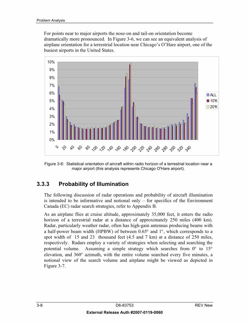
For points near to major airports the nose-on and tail-on orientation become dramatically more pronounced. In Figure 3-6, we can see an equivalent analysis of airplane orientation for a terrestrial location near Chicago’s O’Hare airport, one of the busiest airports in the United States.
0%
1%
2%
3%
4%
5%
6%
7%
8%
9%
10%
0 20 40 60 80100 120 140 160 180 200 220 240 260 280 300 320 340
ALL10'K20'K
Figure 3-6: Statistical orientation of aircraft within radio horizon of a terrestrial location near a major airport (this analysis represents Chicago O'Hare airport).
3.3.3 Probability of Illumination
The following discussion of radar operations and probability of aircraft illumination is intended to be informative and notional only – for specifics of the Environment Canada (EC) radar search strategies, refer to Appendix B.
As an airplane flies at cruise altitude, approximately 35,000 feet, it enters the radio horizon of a terrestrial radar at a distance of approximately 250 miles (400 km). Radar, particularly weather radar, often has high-gain antennas producing beams with a half-power beam width (HPBW) of between 0.65° and 1°, which corresponds to a spot width of 15 and 23 thousand feet (4.5 and 7 km) at a distance of 250 miles, respectively. Radars employ a variety of strategies when selecting and searching the potential volume. Assuming a simple strategy which searches from 0° to 15° elevation, and 360° azimuth, with the entire volume searched every five minutes, a notional view of the search volume and airplane might be viewed as depicted in Figure 3-7.
3-8 D6-83753 REV New
External Release Auth #2007-0119-0060

Problem Analysis
Surface of the EarthRadar
Search Volume(360° azimuth)
Beam Volume
~1°
Surface of the EarthRadar
Search Volume(360° azimuth)
Beam Volume
~1°
Figure 3-7: Horizontal view of an airplane at 35,000 feet altitude entering a radar search volume.
Assume a 1° beam width in azimuth and elevation and assume that the elevation will increment (or decrement) by 1° after each azimuth sweep. Thus, each elevation can be viewed as a ring of 1° elevation over the earth’s surface. As the airplane flies toward the
radar, it will first encounter the 0.5° (centerline) beam elevation, then the 1.5° elevation, and so on. A notional view of this geometry can be seen in Figure 3-8 and
Figure 3-9. Clearly the lower-elevation rings are wider than the higher-elevation rings, and thus they take more time to traverse.
0°
1°2°
Surface of Earth
Aircraft Flight Path
0°
1°2°
Surface of Earth
Aircraft Flight Path
Figure 3-8: A horizontal conceptual view of the elevation rings the airplane flies through in the radar search volume.
17 mi
26 mi
212 mi
154 mi
115 mi
89 mi72 mi
58 mi
39 mi
Assumptions:• 35,000 ft• 600MPH = 10 mi/min• 15 s/scan• 3m 45s /scan volume
5.8 minutes totraverse
1.7 minutes totraverse
9 seconds totraverse
0° 1° 2°Elevation anglebeing scanned
Aircraft Flight Path
17 mi
26 mi
212 mi
154 mi
115 mi
89 mi72 mi
58 mi
39 mi
Assumptions:• 35,000 ft• 600MPH = 10 mi/min• 15 s/scan• 3m 45s /scan volume
5.8 minutes totraverse
1.7 minutes totraverse
9 seconds totraverse
0° 1° 2°Elevation anglebeing scanned
Aircraft Flight Path
REV New D6-83753 3-9
External Release Auth #2007-0119-0060

Problem Analysis
Figure 3-9: A vertical conceptual view of the airplane flying through the radar search volume elevation rings.
One may calculate the density of observations to assess the likelihood of the airplane becoming illuminated by the radar. Assuming that the search strategy is to search the entire volume every 5 minutes, the airplane will be illuminated at least once per five-minute volume scan cycle, except when the airplane is directly overhead (where the radar does not scan). An airplane would take 5.8 minutes to traverse a ring 58 miles wide when flying at 600mph (10 miles a minute). The airplane would be illuminated at least twice during the traversal of the outermost ring – a minimum of once when approaching the radar, and then again in the same ring when departing the radar – with more illuminations highly likely. The airplane is likely to be illuminated about ten times during the 50 minutes it takes for the airplane to traverse the radar search volume. Note that as the airplane gets closer to the radar, the rings become smaller, and eventually the airplane flies out of the search volume over the top of the radar, as seen in
Figure 3-9. The area above the radar scan volume doesn’t reduce the illumination potential much, since it only takes about two minutes to cross the cone.
At long slant ranges the RLAN power levels are lower due to the inverse square law effect, thus interference into the radar by the RLAN is less likely to occur. Likewise, DFS detections are less likely due to low radar power levels. As the airplane approaches the radar the probability of it getting illuminated decreases due to lower residence time in a particular beam, but it has a higher probability of being illuminated by more beams. Also, as the slant range decreases, the path losses decrease, and the signal levels rise for both the radar and the RLAN. This increases the potential for an illumination to trigger the DFS algorithm and for the RLAN to interfere with the radar.
3.3.4 Airborne-Terrestrial Link Budget
The amount of interference into the radar can also be viewed from the perspective of a link budget from the RLAN to the radar. Airborne RLANs are operated at very low power (under 100mW), and the shielding due to the fuselage also reduces the signal levels escaping the aircraft. An analysis of the signal levels emanating from an airframe is shown in Figure 3-10, where the signal levels can be seen to drop below the thermal noise floor at a distance of less than 700 meters.
3-10 D6-83753 REV New
External Release Auth #2007-0119-0060

Problem Analysis
Thermal Noise Floor
FCC Spurious Emissions Limit
-20 dBm
-40 dBm
-60 dBm
-80 dBm
-100 dBm
-120 dBm
-140 dBm
1 m 10 m 100 m 1,000 m 10,000 m 100,000 m
684 m
FuselageAttenuation
~30 m
Distance from Transmitter
Scenario:100 mW 802.11a transmitter17 dB Fuselage Attenuation
SignalStrength
593 m
Thermal Noise Floor
FCC Spurious Emissions Limit
-20 dBm
-40 dBm
-60 dBm
-80 dBm
-100 dBm
-120 dBm
-140 dBm
1 m 10 m 100 m 1,000 m 10,000 m 100,000 m
684 m
FuselageAttenuation
~30 m
Distance from Transmitter
Scenario:100 mW 802.11a transmitter17 dB Fuselage Attenuation
SignalStrength
593 m
Figure 3-10: Depiction of power levels and path loss from an RLAN operating with an airplane.
3.3.5 Impact of Mobility upon DFS Functionality and Efficacy
As noted above, the DFS algorithm is designed around a reasonably fixed radar location, with a fixed RLAN, most likely a consumer installation, in the vicinity. In such a situation, the RLAN, upon powering up would detect the radar within the first radar scan cycle (either during the CAC or during in-service monitoring), change channels to a clear channel, and the configuration would remain static thereafter.
For a mobile platform, such as an airplane traveling at 600mph (1000km/hour), the airplane could pass within tens of radars while on a single flight segment. Based upon the above analysis, the following conclusions concerning proper radar detection may be made:
• To prevent interference into radar systems, the DFS algorithm should scan the appropriate channels for radar signals before use.
• It may be desirable to separate the radar detection function from the transmitting function within the APs, to better manage the switches from one channel to another, and ensure maximum radar detection capability while providing optimal operability of the RLAN.
Next, the performance of DFS-equipped airborne APs in detecting radars is evaluated, and the potential for interference from an airplane into a radar is assessed.
REV New D6-83753 3-11
External Release Auth #2007-0119-0060

Problem Analysis
3-12 D6-83753 REV New
External Release Auth #2007-0119-0060

Test Configuration
4. Test Configuration A Boeing 777-200 airplane was used for these flight tests. The airplane is largely in a commercial revenue configuration (with monuments, seats and stowbins), with the exception of a portion of the central cabin zone which has the standard revenue seats removed and flight test equipment racks installed. This configuration can be seen in Appendix C, which shows the entire airplane layout, including the test equipment rack configuration.
The terrestrial weather radars participating in this collaborative testing are operated by Environment Canada, and are located throughout Canada.
The testing consisted of two flight tests and one ground test, as follows:
• Mt. Sicker flight test, Jun 21 2006 – see Section 5.1 • King site ground test, Aug 9 2006 – see Section 5.2 • Strathmore flight test, Aug 23 2006 – see Section 5.3
During each phase of testing, the RLAN equipment was operated in a couple of different modes. These modes included:
• “Listen-only” mode, in which the AP transmit radios were disabled and DFS radar detections were logged – see Section 4.1.1.
• “RLAN in-service testing” mode, where the APs transmitted RLAN traffic normally and detected radar DFS events in between transmission bursts – see Section 4.1.2.
4.1 Airborne Equipment The APs were installed near the windows on either side of the airplane amidships. The remaining network nodes, traffic generating, performance measuring, and logging equipment were installed in the equipment racks amidships.
The RLAN equipment installed on the airplane consisted of:
• 10 ea. Colubris MAP-330 dual-radio 802.11a/b/g APs • 2 ea Dell laptops, used for syslogging and network traffic generation • Netgear 8-port Ethernet switch
Custom firmware was made available by Colubris (the AP manufacturer) for the purposes of this testing. The firmware details will be outlined below.
As a note: The DFS detection and channel switching policy of the Colubris APs used for the flight tests did not differentiate as to the detected power levels – if the AP detected a radar at any power level, the AP was programmed to execute the DFS algorithm.
REV New D6-83753 4-1
External Release Auth #2007-0119-0060

Test Configuration
4.1.1 Listen-Only Testing
The equipment layout for this DFS flight testing involved two separate configurations. The listen-only mode was designed to allow DFS radar detection in the then-unapproved 5470-5725MHz band without violating any regulatory restrictions or potentially interfering with any radars. This was accomplished by disabling the radio transmitters of the APs, rendering them only able to receive signals, but not to emit any.
The network is depicted in Figure 4-1 below.
Figure 4-1: Equipment configuration for listen-only DFS flight testing.
For the listen-only tests, a custom firmware load for the APs was provided by Colubris for the purposes of this flight testing. The firmware was configured to provide the following functionality:
• Inhibit all transmissions (including BEACONS) • Implement the radar detection component of the proposed FCC DFS algorithm
Note: The radio certification test process for the DFS algorithm had not been released by the FCC at the time of this work, thus the firmware code base and algorithm were not FCC certified.
• Inhibit the DFS channel switching component of the DFS algorithm • Report when the DFS algorithm detects a radar, via syslog (an automatic logging
capability common in network and computer systems management) functionality to a logging laptop computer.
4-2 D6-83753 REV New
External Release Auth #2007-0119-0060

Test Configuration
The airplane was equipped with a sufficient number of APs to simultaneously monitor all 802.11 channels within the frequency bands where DFS is required: 5250-5350MHz and 5470-5725MHz. Thus, with the listen-only configuration, the airplane was able to fly arbitrary flight paths without violating any regulations, and monitor the 5GHz spectrum for radar signals which might disrupt airborne RLAN services.
4.1.2 RLAN In-Service Testing
The second component of the flight testing was to determine the impact of airborne RLANs upon the terrestrial radar system. To accomplish this, a functioning 802.11a AP was required. Since this AP would not execute the DFS channel changing algorithm upon detecting radar, experimental licenses were obtained and all affected agencies consulted, including:
• Industry Canada, the telecommunications agency of Canada, issued an experimental license to transmit in the 5600-5650Mhz band without active DFS functionality enabled.
• Environment Canada, the Canadian weather radar operators, approved the experimental license.
• The US Federal Aviation Administration (FAA) approved the testing. • The US Federal Communications Commission (FCC) approved the testing. • The owner of several C-band radars in northern Washington State, Tribune
Television Northwest, was contacted, and approval granted to potentially interfere with their systems.
The experimentally-licensed network is depicted in Figure 4-2 below.
To enable the in-service testing, the AP vendor supplied a second custom test-only firmware load to Boeing. This firmware provided the following functionality:
• Enable 802.11a RLAN network functionality, including radio transmissions on a selected static channel
• Implement the radar detection component of the proposed FCC DFS algorithm Note: The test process for this algorithm had not been released by the FCC at the time of this testing, thus this firmware code base and algorithm were not FCC certified.
• Inhibit the DFS channel switching component of the DFS algorithm • Report when the DFS algorithm detects a radar, via syslog functionality to a
logging laptop computer
For this test, EC radars were selected which operated within 802.11a channel 124 (5610-5630MHz), therefore a single AP was required to transmit. The AP was configured to maximum power output, which is listed as 18dBm, or approximately 65mW. A standard “rubber ducky” dipole antenna was oriented longitudinally along the axis of the fuselage.
Since a two-way network link between AP and the client would not be possible without acquiring an experimental client as well, the decision was made to provide a network load to the AP via multicast transmissions (which do not require
REV New D6-83753 4-3
External Release Auth #2007-0119-0060

Test Configuration
acknowledgments from a receiving system, and thus no receiver). The tool used to generate the traffic was Iperf (http://dast.nlanr.net/Projects/Iperf/).
Figure 4-2: Equipment configuration for transmitting DFS flight testing.
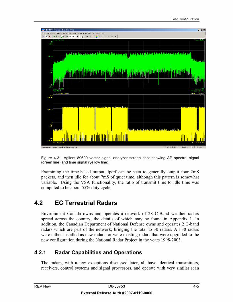
To adequately assess the AP’s ability to simultaneously conduct network operations and monitor for radars, Iperf was configured to supply network traffic of 3Mbps. The multicast signaling rate for APs was configured to 6Mbps. A vector signal analyzer (VSA) plot is shown in Figure 4-3, where the green line is the power output across frequency, and the yellow line represents power output as a function of time.
4-4 D6-83753 REV New
External Release Auth #2007-0119-0060
Test Configuration
Figure 4-3: Agilent 89600 vector signal analyzer screen shot showing AP spectral signal (green line) and time signal (yellow line).
Examining the time-based output, Iperf can be seen to generally output four 2mS packets, and then idle for about 7mS of quiet time, although this pattern is somewhat variable. Using the VSA functionality, the ratio of transmit time to idle time was computed to be about 55% duty cycle.
4.2 EC Terrestrial Radars Environment Canada owns and operates a network of 28 C-Band weather radars spread across the country, the details of which may be found in Appendix 1. In addition, the Canadian Department of National Defense owns and operates 2 C-band radars which are part of the network; bringing the total to 30 radars. All 30 radars were either installed as new radars, or were existing radars that were upgraded to the new configuration during the National Radar Project in the years 1998-2003.
4.2.1 Radar Capabilities and Operations
The radars, with a few exceptions discussed later, all have identical transmitters, receivers, control systems and signal processors, and operate with very similar scan
REV New D6-83753 4-5
External Release Auth #2007-0119-0060

Test Configuration
sequences and data processing. The radars operate 24/7, all year long, with occasional (generally less than 2% per year) downtime for maintenance. The radar data are sent over network links to regional and national forecast centers where they are converted into image products for use by forecasters, special users (e.g. the aviation community, broadcasters) and by the general public.
4.2.1.1 Radar Antennas The main difference among the radars is the size and gain of the antennas. Eleven of the radars have large 6.1m diameter antennas with a one way gain of 49.2 dBi and a HPBW of 0.62 degrees. Eighteen of the radars have 3.6m diameter antennas (42.9 dBi gain, 1.1 deg HPBW), and one radar has a small 2.4m diameter antenna (41.5 dBi gain, 1.63 deg HPBW). A sample radar antenna radiation pattern may be seen in Figure 4-4 (this is the King Station radar antenna), with a close-up view of the main lobe shown in Figure 4-5.
Appendix A lists for each radar site: the radar name, three letter designator, latitude, longitude, height of the antenna mid point, operating frequency, and antenna gain.
The antenna/pedestal sits atop a steel tower whose height was chosen so that the antenna is higher than nearby obstructions such as trees. Prairie sites tend to have tower heights around 12m, and heavily forested sites have tower heights up to 27m. Several of the sites (XME, XAM, XSS and XSI) are located on the tops of mountains.
The antennas can rotate through 360 degrees in azimuth at speeds between 0.5 deg/sec and 36 deg/sec and can also be pointed at any specific azimuth angle. In elevation, the antenna can be pointed between about -2.0 deg and +60.0 deg for the 3.6m antennas and +90.0 degrees for the 6.1m antennas. The elevation speed can be up to +/- 15 deg/sec. Most of the radar data are collected at speeds of 5 deg/sec or 36 deg/sec and at elevation angles between 0.0 and +24.6 degrees. A few of the mountain top sites will use elevation angles below 0.0 degrees to look down into a valley.
4-6 D6-83753 REV New
External Release Auth #2007-0119-0060

Test Configuration
King Radar Antenna Pattern
-90-80-70-60-50-40-30-20-10
0
-180 -150 -120 -90 -60 -30 0 30 60 90 120 150 180
Azimuth Angle (Deg)
Nor
mal
ized
Gai
n (d
B)
Figure 4-4: Radar antenna radiation pattern for King Station radar.
King Radar Antenna Main Lobe
-60
-50
-40
-30
-20
-10
0
-5 -4 -3 -2 -1 0 1 2 3 4 5Azimuth Angle (Deg)
Nor
mal
ized
Gai
n (d
B)
Figure 4-5: Magnified view of the King Station radar antenna main lobe.
4.2.1.2 Radar Transmitter and Receiver The transmitters use a CPI SFD-373 magnetron as the microwave power tube. The nominal output power of the tube is 250 kw peak with a maximum duty cycle of 0.001. The modulator is configured for three different pulse widths: 2.0 usec, 1.6 usec and 0.8 usec. The maximum pulse repetition frequency (prf) that is used at each pulse width is 250 pps at 2.0 usec, 600 pps at 1.6 usec and 1200 pps at 0.8 usec.
REV New D6-83753 4-7
External Release Auth #2007-0119-0060

Test Configuration
The receiver has a bandwidth that is matched to the pulse width in use, typically about 0.5 MHz at 2.0 usec, 0.7 MHz at 1.6 usec and 1.0 MHz at 0.8 usec. As can be seen in Appendix A, all of the transmitters operate in the band 5600 to 5650 MHz.
The transmit frequency for a given site has been chosen so that nearby radar sites do not interfere with each other. The exact transmit frequency may vary by about 1MHz from the values in the table because the frequency is a function of the temperature of the magnetron tube. An Automatic Frequency Control (AFC) loop monitors the transmit frequency and adjusts the frequency of the Stable Local Oscillator such that the Intermediate Frequency into the receiver remains at 30 MHz +/- 50 kHz.
4.2.1.3 Radar Processor All 30 radars are controlled by computers which are accessible over the Environment Canada internal network. The control software and hardware is a fairly common commercially available weather radar control system developed and supplied by Sigmet/Vaisala Inc. Specifically, Sigmet IRIS is the control and data acquisition software, an RCP02 Radar Control Processor controls the transmitter and antenna, and an RVP-7 Signal Processor takes the raw IF signal from the receiver and converts it to digital bytes of reflectivity, radial velocity and spectral width from specific range bins (a volume of space defined by range, azimuth angle and elevation angle from the radar site).
4.2.1.4 WKR King Site The ground test data in this report was collected at the WKR King site, and it is worth mentioning at this point that King is a combined research and operations radar and differs from the other sites in that it is the only dual-polarization radar. The other 29 radars use linear horizontal polarization for transmit and receive power, but King has the ability to operate with horizontal polarization or to split the transmit power equally into two channels, one with horizontal polarization and the other with vertical polarization. King has two matched receivers, one for the horizontal channel and one for the vertical channel. King also uses the next generation of hardware from Sigmet/Vaisala; an RCP8 instead of an RCP02 and an RVP8 instead of an RVP7.
4.2.2 General Scan Strategy
A rather complex antenna scan strategy and radar and signal processing configuration has been developed to optimize the collection of useful data in a minimum amount of time. It would be desirable to measure everything, everywhere, all the time; but in practice the pulse width, the pulse repetition frequency, the antenna rotation speed, the elevation angle, the width of the range bins, the length of the range bins and the signal processing algorithm must be balanced and optimized, including averaging and thresholding. With a longer pulse width, smaller precipitation rates can be detected, but the equipment must operate at a lower pulse repetition rate so as not to overload
4-8 D6-83753 REV New
External Release Auth #2007-0119-0060

Test Configuration
the transmit tube. Lower pulse repetition rates give fewer samples for averaging. For the measurement of radial velocity, high pulse repetition rates are needed, but that reduces the available pulse width hence the sensitivity is not as good.
All the sites except WKR King currently use the general scan strategy, which repeats every 10 minutes: The dual-polarization site (WKR King) currently uses a slightly different scan strategy in order to collect some dual-polarization data.
Details of the scan strategies may be found in Appendix B.
REV New D6-83753 4-9
External Release Auth #2007-0119-0060

Test Configuration
4-10 D6-83753 REV New
External Release Auth #2007-0119-0060

Test Chronology and Results
5. Test Chronology and Results
5.1 Mt. Sicker Flight Test To assess the impact of airborne RLANs upon operational radars, a flight test was planned in cooperation with Environment Canada around EC’s Mt. Sicker weather radar located on the southern end of Vancouver Island. The objectives of this flight test were to:
• Assess the radar detection performance of an airborne AP • Assess the reported radar power levels detected by the AP • Assess the radar interference due to airborne RLANs, which operated
continuously without regard to DFS detections
5.1.1 Test Configuration and Procedures
The flight test airplane launched from the United States, and flew to Vancouver BC. Upon reaching the vicinity of the EC Mt Sicker radar, the airplane flew a specific flight path designed to maximize the potential for radar illumination, and enable accurate measurements. All flight legs near the radar were flown at 25,000 feet altitude (MSL – Mean Sea Level) (7620m). Specifically, the flight encompassed the following flight legs around the radar site:
• Upon arriving in the vicinity, a tangent to a circle of radius 50 nautical miles (nm) (92.6km)
• A semi-circle at constant altitude and distance from the radar at a 50-nm (92.6km) radius.
• A tangent to a circle of 25-nm (46.3km) radius around the radar • A semi-circle at constant altitude at a 25-nm (46.3km) radius. • Passing directly over the radar, flying directly away from the radar for a distance
of approximately 150 nm (277.8km), then returning directly overhead.
A map with the flight tracks, plotted in Figure 5-1, shows each of these flight legs.
The flight paths were selected to:
• Semi-circles: force the airplane to dwell within clear sight of the radar without changing azimuth or elevation with respect to the airplane. This eliminates the variable of changing fuselage attenuation, and provides the radar a clear view into the cabin through the windows. The 25-mile circle provides opportunities for the lowest reasonable slant range path loss measurements. At shorter slant ranges, the elevation uptilt of the radar antenna becomes increasingly unlikely.
• Tangents: Assess the more realistic condition of having an airplane flying past a radar. This path also exercises various aircraft azimuth and elevation angles, which provide variability in fuselage losses.
REV New D6-83753 5-1
External Release Auth #2007-0119-0060

Test Chronology and Results
5-2 D6-83753 REV New
External Release Auth #2007-0119-0060
• Directly towards/away from radar: confirm that nose-on and tail-on orientations have sufficient shielding, in spite of the short slant ranges.
5.1.2 Airborne DFS Detection Results
After taking off from Glasgow Montana the listen-only RLAN equipment was powered up. After flying into Canadian airspace, the transmit-capable RLAN equipment was powered up in accordance with the experimental license conditions.
The APs recorded DFS detections by issuing a syslog record, which showed the channel number and the received power that the AP detected. Note that the AP radios are not calibrated, and the received power is calculated from the RSSI (received signal strength indication). The accuracy of this received power calculation is known to be somewhat non-linear and thus is not accurate. The APs report received signal powers down to approximately -80dBm.
During the course of the flight test, the airborne APs registered a number of radar detections, which can be attributed to Canadian radar systems in the vicinity. A map of the total flight path from Montana to Vancouver is shown in Figure 5-2. The map is annotated with the EC radar sites, blue dots to indicate DFS detections with radar power above the FCC regulatory limit of -62dBm, and green flags to indicate DFS detections above a -50dBm threshold. Note that qualitatively, the most significant “hits” are approximately 10 minutes apart corresponding to a direct illumination by the radar beam for every complete cycle of the 10 minute radar scan cycle, as expected. This data represent output from the “listen-only” APs. Based upon link budget calculations in [1] and [2], if the AP detects the radar at above -50dBm, then the radar is at a distance where it should be able to “see” the AP transmitted signal.
As would be expected, during the directed flight test flight segments very close to the radar, the number of radar detections increased. In Figure 5-3 the details of the flight segments, annotated with the DFS detections are shown. Additional details on the detections are collated in Table 5-1, including power received and aircraft position.
As can be seen in the plots, the DFS algorithm does detect radars as the beams sweep past and illuminate the airplane. Due to the statistical uncertainty of aircraft illumination while within the search volume, there is no expectation that the radar detections would have a strong correspondence to the shortest distance between the airplane and the radar.

Test
Chr
onol
ogy
and
Res
ults
Figu
re 5
-1:
Flig
ht te
st tr
acks
follo
wed
in th
e vi
cini
ty o
f Mt S
icke
r rad
ar s
ite.
RE
V N
ew
D6-
8375
3 5-
3
Exte
rnal
Rel
ease
Aut
h #2
007-
0119
-006
0

Test
Chr
onol
ogy
and
Res
ults
Figu
re 5
-2:
Flig
ht p
ath
from
Gla
sgow
Mon
tana
to M
t Sic
ker,
BC
rada
r site
. B
lack
dot
s in
dica
te fl
ight
pat
h, b
lue
dots
are
rada
r det
ectio
ns
abov
e th
e FC
C re
gula
tory
-62d
Bm
thre
shol
d, g
reen
flag
s ar
e ra
dar d
etec
tions
abo
ve a
-50d
Bm li
mit.
5-4
D6-
8375
3 R
EV
New
Exte
rnal
Rel
ease
Aut
h #2
007-
0119
-006
0

Test
Chr
onol
ogy
and
Res
ults
Figu
re 5
-3:
Det
ails
of f
light
pat
h ar
ound
Mt.
Sic
ker r
adar
site
with
DFS
pow
er re
adin
gs a
nnot
ated
. B
lack
dot
s in
dica
te fl
ight
pat
h, b
lue
dots
ar
e ra
dar d
etec
tions
abo
ve th
e FC
C re
gula
tory
-62d
Bm
thre
shol
d, g
reen
flag
s ar
e ra
dar d
etec
tions
abo
ve a
-50d
Bm
lim
it.
RE
V N
ew
D6-
8375
3 5-
5
Exte
rnal
Rel
ease
Aut
h #2
007-
0119
-006
0

Test
Chr
onol
ogy
and
Res
ults
5-6
D6-
8375
3 R
EV
New
Exte
rnal
Rel
ease
Aut
h #2
007-
0119
-006
0
Tabl
e 5-
1: D
FS ra
dar d
etec
tion
deta
ils fr
om li
ght p
ath
map
flag
ged
(gre
en fl
ags)
eve
nts
.24
996.
01-1
23.4
3549
.029
5112
456
20-4
9AP
183:
27:4
7 PM
26
2502
7-1
23.4
0849
.033
3612
456
20-4
6AP
183:
27:3
3 PM
25
2494
6.96
-123
.318
49.0
5211
124
5620
-47
AP18
3:26
:45
PM24
2494
6.96
-123
.318
49.0
5211
124
5620
-44
AP18
3:26
:45
PM23
2500
4.97
-124
.074
49.1
5048
124
5620
-41
AP18
3:20
:50
PM22
2501
8.96
-124
.79
48.7
6126
124
5620
-46
AP18
2:38
:35
PM21
2500
6.96
-124
.718
48.7
5291
124
5620
-44
AP18
2:37
:56
PM20
2500
4.05
-124
.688
48.8
2953
124
5620
-45
AP18
2:36
:53
PM19
2500
5.98
-124
.24
49.5
1961
124
5620
-48
AP18
2:26
:46
PM18
2500
5.97
-124
.221
49.5
2287
124
5620
-45
AP18
2:26
:36
PM17
2500
5.02
-123
.277
49.6
6776
124
5620
-40
AP18
2:18
:31
PM16
2500
4.02
-123
.257
49.6
6667
124
5620
-39
AP18
2:18
:21
PM15
2500
5-1
23.2
1649
.664
4912
456
20-4
8AP
182:
18:0
1 PM
14
3141
7.1
-122
.272
49.6
1024
124
5620
-50
AP18
2:11
:31
PM13
3436
4.2
-121
.676
49.5
7179
124
5620
-49
AP18
2:08
:04
PM12
3801
3-1
19.8
1449
.570
3712
456
20-4
9AP
181:
57:4
3 PM
11
3799
4-1
19.6
9949
.571
6912
456
20-4
8AP
181:
57:0
5 PM
10
3800
1.01
-118
.089
49.5
7809
124
5620
-37
AP18
1:48
:24
PM9
3799
8.04
-116
.917
49.5
6865
124
5620
-42
AP18
1:42
:11
PM8
3800
2.98
-116
.259
49.5
584
124
5620
-46
AP18
1:38
:43
PM7
3799
4.06
-114
.992
49.4
978
124
5620
-45
AP18
1:32
:01
PM6
3800
2-1
14.3
3549
.458
512
456
20-4
9AP
181:
28:3
1 PM
5
3800
7-1
14.3
0449
.456
612
456
20-4
7AP
181:
28:2
1 PM
4
3799
2-1
12.3
3649
.315
6712
456
20-4
7AP
181:
17:5
3 PM
3
3799
8.02
-111
.364
49.2
3328
124
5620
-48
AP18
1:12
:45
PM2
3799
8.02
-111
.364
49.2
3328
124
5620
-40
AP18
1:12
:45
PM1
Alt
Long
Lat
chan
num
chan
freq
Rx
Pow
erAP
Nam
eTi
me(
sec)
Even
t #
2499
6.01
-123
.435
49.0
2951
124
5620
-49
AP18
3:27
:47
PM26
2502
7-1
23.4
0849
.033
3612
456
20-4
6AP
183:
27:3
3 PM
25
2494
6.96
-123
.318
49.0
5211
124
5620
-47
AP18
3:26
:45
PM24
2494
6.96
-123
.318
49.0
5211
124
5620
-44
AP18
3:26
:45
PM23
2500
4.97
-124
.074
49.1
5048
124
5620
-41
AP18
3:20
:50
PM22
2501
8.96
-124
.79
48.7
6126
124
5620
-46
AP18
2:38
:35
PM21
2500
6.96
-124
.718
48.7
5291
124
5620
-44
AP18
2:37
:56
PM20
2500
4.05
-124
.688
48.8
2953
124
5620
-45
AP18
2:36
:53
PM19
2500
5.98
-124
.24
49.5
1961
124
5620
-48
AP18
2:26
:46
PM18
2500
5.97
-124
.221
49.5
2287
124
5620
-45
AP18
2:26
:36
PM17
2500
5.02
-123
.277
49.6
6776
124
5620
-40
AP18
2:18
:31
PM16
2500
4.02
-123
.257
49.6
6667
124
5620
-39
AP18
2:18
:21
PM15
2500
5-1
23.2
1649
.664
4912
456
20-4
8AP
182:
18:0
1 PM
14
3141
7.1
-122
.272
49.6
1024
124
5620
-50
AP18
2:11
:31
PM13
3436
4.2
-121
.676
49.5
7179
124
5620
-49
AP18
2:08
:04
PM12
3801
3-1
19.8
1449
.570
3712
456
20-4
9AP
181:
57:4
3 PM
11
3799
4-1
19.6
9949
.571
6912
456
20-4
8AP
181:
57:0
5 PM
10
3800
1.01
-118
.089
49.5
7809
124
5620
-37
AP18
1:48
:24
PM9
3799
8.04
-116
.917
49.5
6865
124
5620
-42
AP18
1:42
:11
PM8
3800
2.98
-116
.259
49.5
584
124
5620
-46
AP18
1:38
:43
PM7
3799
4.06
-114
.992
49.4
978
124
5620
-45
AP18
1:32
:01
PM6
3800
2-1
14.3
3549
.458
512
456
20-4
9AP
181:
28:3
1 PM
5
3800
7-1
14.3
0449
.456
612
456
20-4
7AP
181:
28:2
1 PM
4
3799
2-1
12.3
3649
.315
6712
456
20-4
7AP
181:
17:5
3 PM
3
3799
8.02
-111
.364
49.2
3328
124
5620
-48
AP18
1:12
:45
PM2
3799
8.02
-111
.364
49.2
3328
124
5620
-40
AP18
1:12
:45
PM1
Alt
Long
Lat
chan
num
chan
freq
Rx
Pow
erAP
Nam
eTi
me(
sec)
Even
t #

Test Chronology and Results
5.1.3 Listen-Only vs. In-Service DFS Detection Results
The current generation of APs has an intrinsic limitation in which they cannot simultaneously receive and transmit. When assessing the performance of the DFS detections, one might expect the detection performance to degrade when the radio is attempting to transmit a significant amount of data at the same time it is monitoring for the presence of a radar. This would be expected, since it is impossible for the AP to be able to listen for a radar while it is transmitting data.
To determine the limitations of an in-service AP, the experimental RLAN was configured with two independent APs – one operating in listen-only mode, the other in functional network service. A comparison of the two AP’s ability to detect radars can be seen in Figure 5-4, where the in-service AP can be seen to suffer some performance impairments (as would be well expected), but still be capable of detecting radars.
1
10
100
1000
14:15 14:35 14:55 15:15 15:35 15:55 16:15 16:35
Time (hr:min)
Cou
nt o
f DFS
Det
ectio
ns
Listen-Only
In-Service
Figure 5-4: A comparison between listen-only and in-service AP radar detection rates during flight test over Mt Sicker. Scatter-plot dots represent the count of DFS detections over the
FCC limit of -62dBm obtained from each AP in 5-minute bins during the flight test.
REV New D6-83753 5-7
External Release Auth #2007-0119-0060

Test Chronology and Results
5.1.4 Weather Radar Interference Results
5.1.4.1 Configuration for Flight Test For the flight on 21 Jun, all EC radars, with the exception of Mt Sicker (XSI), were running the standard scan strategy from Appendix B.
The Mt Sicker configuration was optimized to enhance the effectiveness of the flight tests.
• The “Speckle Filter” was turned off in the radar signal processor. This allowed isolated bins, i.e. a bin without a neighbor either in range or in azimuth, to be passed into the product. (Normally the speckle filter rejects any returns which do not occur in multiple bins in an effort to eliminate the effects of airplanes flying through the search volume.)
• The Doppler tasks in Appendix B (Dopvol_1 and Dopvol2) were turned off and were replaced with a new task similar to CONVOL, but with the top three elevation angles deleted in order to reduce the duration of the task to about 4 minutes 30 seconds. It was necessary to delete the three highest elevation scans to finish the complete volume scan in less than five minutes.
• The CONVOL task for XSI uses elevation angles that are all 0.2 degrees lower than the CONVOL angles in Appendix B because XSI is a mountain top site. Thus the XSI CONVOL elevation angles are 24.4 to 0.1 instead of the standard 24.6 to 0.3.
5.1.4.2 RLAN Interference into Radar Results The reflectivity data in PPI displays for all of the elevation angles (“tilts”) collected during the 21 Jun 2006 flight for both the Mt Sicker (XSI) and Aldergrove (WUJ) radars have been examined. No interference that would be attributable to an RLAN operating with a 2 millisecond transmit time and a 180 microsecond backoff time was found.
5.1.5 Conclusions from Mt. Sicker Flight Test
In conclusion, this flight test campaign has shown that
• The US-developed DFS algorithm continues to function in a high-speed platform. The velocity of the mobile network doesn’t impact the functionality of the algorithm in any noticeable way.
• The airborne RLAN did not apparently interfere with the EC weather radars, in spite of worst-case configurations and flight paths.
The results that the DFS algorithm works well at speed are expected. Computing the potential Doppler shift in frequencies due to aircraft velocity results in numbers well
5-8 D6-83753 REV New
External Release Auth #2007-0119-0060
Test Chronology and Results
within the resolution bandwidths of both radars and 802.11 RLANs, and thus should not be a factor in DFS functionality.
On the other hand, the lack of apparent interference into the radar was somewhat unexpected and disconcerting. This result was surprising because the airborne DFS algorithm reported radar power as high as -40 dBm and expectations were that, within a few dB, if the RLAN could see the radar, then the radar could see the RLAN. Consequently a decision was made to explore this discrepancy further.
5.2 King Site Ground Test To validate results from the Mt. Sicker flight tests, and to explore the gaps between expectations and experimental results, ground testing was conducted using the flight test APs and the EC King City radar.
The major objectives of the testing were:
• Assess the performance of the DFS algorithm when subjected to Canadian weather radar systems. This was the first attempt to validate actual DFS implementation in a commercial AP against Canadian radar.
• Confirm amounts of interference caused by terrestrial commercial APs operating in radar frequency bands.
5.2.1 Test Procedures
The same APs and firmware loads were used as on the airplane, as were the regulatory licensing arrangements. The APs were operated in listen-only mode, and also in transmit mode during various stages of the testing. As before, DFS detection events were recorded using syslog functionality. The radar recorded the AP transmission, using a constant elevation sweep of the radar antenna.
Testing was conducting in the following scenarios:
• Bench testing in the radar building computer room with the radar operating in various modes
• External testing in listen-only mode, to correlate the AP DFS events with radar operations
• External testing in transmit mode, to confirm link budget calculations and radar interference issues
Also tested were a variety of other potential variables, to assess the impact upon DFS performance in the real world. Variables tested included:
• Adjacent 802.11 channel DFS detection rate. • AP antenna polarization • Radar azimuth rotation rate variations, from “staring mode” (0 deg/s) to very high
scan rates (36 deg/s) • Radar elevation changes
REV New D6-83753 5-9
External Release Auth #2007-0119-0060

Test Chronology and Results
• Radar transmit on/off • Various pulse lengths, from 0.8µs to 2µs • Various pulse repetition frequencies (PRFs), dual and single PRFs
5.2.2 Bench Testing
The AP was operated in listen-only mode in the radar building as part of the initial equipment check out procedure. The AP was situated less than 3 m from the transmitter cabinet as seen in Figure 5-5. The radar antenna was on a tower 30 m above the building. Surprising to the radar operators, the AP recorded DFS events at power levels around -60 to -40 dBm, with a periodic pattern corresponding to the antenna rotation rate and direction. To confirm that the “hits” were due to the radar, the transmitter was cycled on and off. When the transmitter was off, the hits disappeared, as seen in Figure 5-6, providing clear evidence of the operability of the DFS.
Figure 5-5: Bench testing the AP in the King Site radar control room.
5-10 D6-83753 REV New
External Release Auth #2007-0119-0060
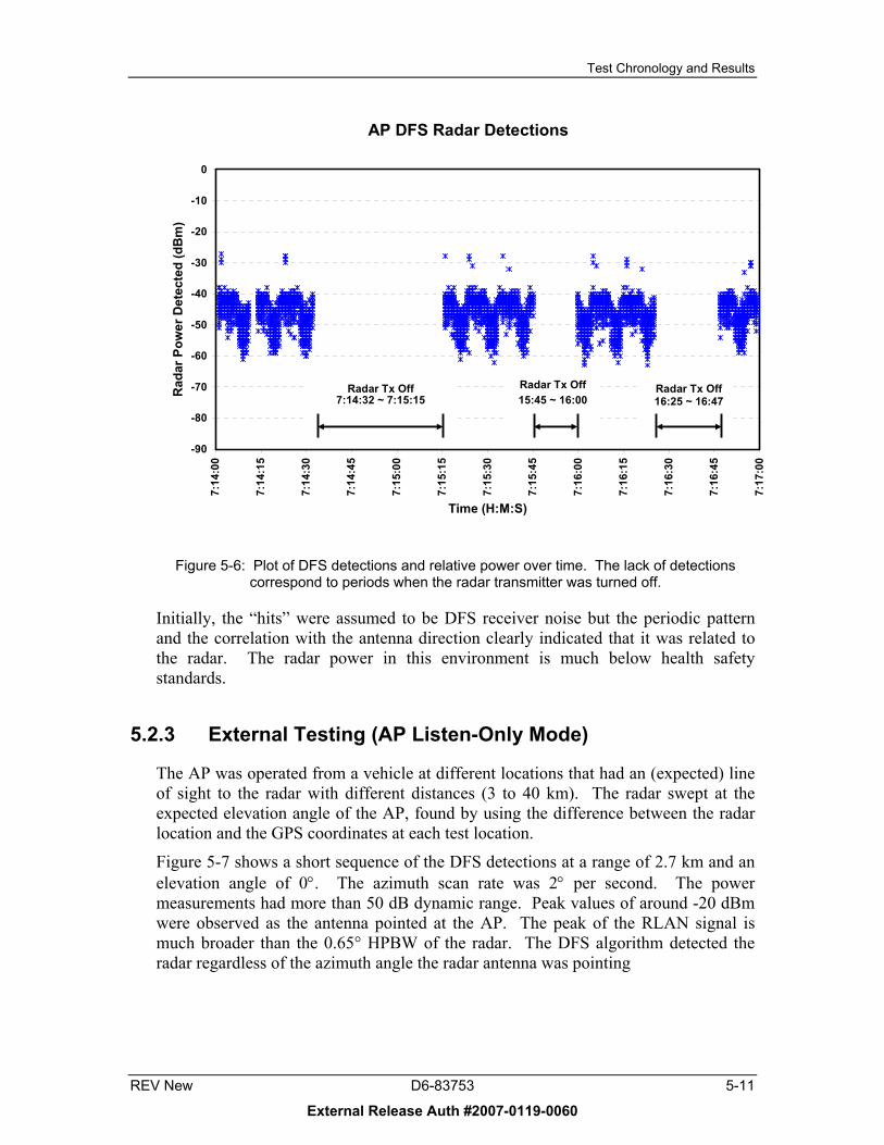
Test Chronology and Results
AP DFS Radar Detections
-90
-80
-70
-60
-50
-40
-30
-20
-10
0
7:14
:00
7:14
:15
7:14
:30
7:14
:45
7:15
:00
7:15
:15
7:15
:30
7:15
:45
7:16
:00
7:16
:15
7:16
:30
7:16
:45
7:17
:00
Time (H:M:S)
Rad
ar P
ower
Det
ecte
d (d
Bm
)
Radar Tx Off7:14:32 ~ 7:15:15
Radar Tx Off15:45 ~ 16:00
Radar Tx Off16:25 ~ 16:47
Figure 5-6: Plot of DFS detections and relative power over time. The lack of detections correspond to periods when the radar transmitter was turned off.
Initially, the “hits” were assumed to be DFS receiver noise but the periodic pattern and the correlation with the antenna direction clearly indicated that it was related to the radar. The radar power in this environment is much below health safety standards.
5.2.3 External Testing (AP Listen-Only Mode)
The AP was operated from a vehicle at different locations that had an (expected) line of sight to the radar with different distances (3 to 40 km). The radar swept at the expected elevation angle of the AP, found by using the difference between the radar location and the GPS coordinates at each test location.
Figure 5-7 shows a short sequence of the DFS detections at a range of 2.7 km and an elevation angle of 0°. The azimuth scan rate was 2° per second. The power measurements had more than 50 dB dynamic range. Peak values of around -20 dBm were observed as the antenna pointed at the AP. The peak of the RLAN signal is much broader than the 0.65° HPBW of the radar. The DFS algorithm detected the radar regardless of the azimuth angle the radar antenna was pointing
REV New D6-83753 5-11
External Release Auth #2007-0119-0060

Test Chronology and Results
AP DFS Radar Detections
-90
-80
-70
-60
-50
-40
-30
-20
-10
0
15:42 15:43 15:44 15:45 15:46 15:47 15:48 15:49 15:50 15:51 15:52
Time (H:M)
Rad
ar P
ower
Det
ecte
d (d
Bm
)
Figure 5-7: AP DFS detections in the field at a range of 2.7km. Radar was scanning azimuth at 2° per second with a constant elevation angle of 0°. The peaks of detection power correspond to when the radar was pointing directly at the AP.
To explore this a little more, the radar scan rate was increased to 36° per second, and the antenna elevation angle was raised step-wise from 5 o to 35o in 5 o increments once per minute. Figure 5-8 shows the corresponding DFS hits reported by the AP. The peak power decreased as the elevation increased away from the on-target elevation angle (0o) whereas the base levels remain the same. This clearly illustrates that the DFS detects the weather radar even on off-axis directions. The DFS is either seeing signal directly from the antenna or off multiple scattering mechanisms.
5-12 D6-83753 REV New
External Release Auth #2007-0119-0060

Test Chronology and Results
AP DFS Radar Detections
-100
-90
-80
-70
-60
-50
-40
-30
-20
16:22 16:23 16:24 16:25 16:26 16:27 16:28 16:29
Time (H:M)
Rad
ar P
ower
Det
ecte
d (d
Bm
)
5° 10° 15° 20° 25° 30° 35°
Radar Antenna Elevation Angle
Figure 5-8: AP DFS detections as radar antenna elevation angle is swept between 5 and 35 degrees. AP was located 2.7km away from radar.
As the distance between the AP and the radar increased, the ability of the AP to detect the radar via multipath or the antenna backlobes degraded. At the farthest range of the test (~48km), the peak signal could still be identified whereas the off–axis hits decreased significantly, as seen in Figure 5-9.
Another question of interest was the prevalence of false positive radar detection. While at the furthest range, the radar transmitter was cycled on and off on 30 second intervals, starting at 16:08. As shown in Figure 5-9, the AP generally did not generate false positives, however, it would continue to output log entries for prior detections for several seconds after the radar was no longer visible.
REV New D6-83753 5-13
External Release Auth #2007-0119-0060

Test Chronology and Results
AP DFS Radar Detections
-90
-80
-70
-60
-50
-40
-30
-20
-10
0
16:0
7:30
16:0
7:45
16:0
8:00
16:0
8:15
16:0
8:30
16:0
8:45
16:0
9:00
16:0
9:15
16:0
9:30
16:0
9:45
16:1
0:00
Time (H:M:S)
Rad
ar P
ower
Det
ecte
d (d
Bm
)
Radar Tx Off Radar Tx Off09:00 ~ 09:3008:00 ~ 08:30
Figure 5-9: AP DFS detections at a range of 48km. It can take up to 5 seconds for the AP to stop reporting a radar signal after the signal is removed.
Longer range tests were not conducted due to time constraints. Locations were chosen where good line of sight was expected and so these should be interpreted as near-worse case scenarios. Of course, the results are dependent on the local conditions of the location, intervening terrain and atmospheric propagation conditions.
5.2.4 Additional Comments on Listen-Mode Tests
In addition, the AP performed DFS monitoring on adjacent channels to the radar operation. The AP did not detect the radar when monitoring adjacent 802.11 channels. No DFS events during the monitoring period could be attributed to the test radar when monitoring the first and second adjacent channels.
It is important to note that the AP reporting of radar signal power levels was, at best, an approximation. The manufacturer advised that the received signal strength indicator (RSSI) was used to compute the reported radar power. Upon reviewing link budget analysis and reported signal strengths, however, it became clear that the AP radio must have some type of automatic gain control (AGC) functionality altering the reported signal levels dynamically.
In the ground test, the DFS was able to detect the weather radar out to the maximum measured range (~47 km). Figure 5-10 shows the radar power received by the AP.
5-14 D6-83753 REV New
External Release Auth #2007-0119-0060

Test Chronology and Results
These values are the maximum reported values at the indicated range. Presumably, these occur when the radar is directly incident on the AP. It was expected that the path loss exponent (PLE) would roughly be related to the free space value of 2 (red line). A previous related study [1] reported a PLE of 2.28 for terrestrial RLAN systems. Here the value is about 0.95 which is interpreted as a non-linear effect, probably due to signal enhancement using AGC or some other technique. There is a hint of a sawtooth pattern indicative of AGC.
Figure 5-10: Comparison between expected and observed AP reports of radar power. Red line is expected value, with a path loss exponent (PLE) of 2, while the black line is the observed roll-off of AP power reports.
5.2.5 External Testing (AP Transmit Mode)
The AP was operated in transmit mode at 3 locations (2.7, 6.4 and 16.7 km). The antenna of the AP was varied from horizontal to vertical positions and in between. The radar elevation angle was set at the expected incident angle on the AP.
Below are two examples of RLAN interference into the radar shown as a PPI display. Figure 5-11 shows the impact of an AP at a range of 6.7 km, and Figure 5-12 shows the impact at a 16.8 km range. The data was collected without any filtering and the images show ground clutter echoes near the radar (center of image). The RLAN signal shows up as long radials of constant power.
REV New D6-83753 5-15
External Release Auth #2007-0119-0060

Test Chronology and Results
Figure 5-11: Interference into the radar from an AP transmitting at a range of 6.4km.
Figure 5-12: Interference into the radar from an AP transmitting at a range of 16.7km.
It is possible to represent the interference signal as a single radial from the radar location, looking out over all range bins. In Figure 5-13, the data is presented as the
5-16 D6-83753 REV New
External Release Auth #2007-0119-0060

Test Chronology and Results
radar reflectivity factor and in Figure 5-14, the data is presented as received power. The “radar reflectivity factor,” measured in units of dBZ, is a common unit for weather radar data. The dBZ unit of measurement contains factors which compensate for the decreasing return due to distance, oxygen attenuation, and differences in various radars.
The spikes in the data are due to reflections from local ground targets. Figure 5-14 shows that the RLAN is observed as constant power source extending to all ranges. The perception of increasing return in Figure 5-13 is due to the dBZ approach to normalizing the power return to a target density per unit volume. The appearance of the RLAN signal over all range bins is due to the very long packet lengths (over 2ms) of the RLAN signal look like a 200km-long target to the radar.
AP Interference Levels into Radar in dBZ
-60
-40
-20
0
20
40
60
0 50 100 150 200 250
Slant Range (km)
Rec
eive
d Si
gnal
(dB
Z)
AP Signal LevelRadar Noise Floor
REV New D6-83753 5-17
External Release Auth #2007-0119-0060

Test Chronology and Results
Figure 5-13: Apparent AP reflectivity return over range bins as observed by the radar. The reflectivity increases over distance due to dBZ normalization.
Figure 5-14: AP power received in radar processor over range bins. The received power appears to be constant over all range bins because it actually is sourced at only one location, and thus is constant.
In
Figure 5-15, a summary of the RLAN power measurements taken at different distances from the radar (3 to 16 km) are presented. The RLAN had two omni-directional (monopole) antennas that each could be manually oriented horizontally or vertically. In a free-space environment, it would be expected that the received power measurements taken by the radar would decrease with range. In this practical situation, however, the results do not show this. The power measurements at 3 km and 16 km are approximately the same and the measurements at 7 km are about 10 to 20 dB higher than the other two. This variation is most likely due to terrain blockage, multi-path, and propagation conditions dominating the range effect. While there was some variation with antenna orientation at a particular site, the results were inconsistent at the various ranges.
AP Interference Level into Radar in dBm
-120
-100
-80
-60
-40
-20
0
0 50 100 150 200 250
Slant Range (km)
Rec
eive
d Po
wer
(dB
m)
AP Signal LevelRadar Noise Floor
5-18 D6-83753 REV New
External Release Auth #2007-0119-0060

Test Chronology and Results
Figure 5-15: RLAN power received at the radar by distance and AP antenna polarization.
REV New D6-83753 5-19
External Release Auth #2007-0119-0060
Test Chronology and Results
5.2.6 Conclusions from Ground Testing
The results from the ground testing were extremely encouraging – the DFS is very sensitive, and the DFS algorithm functioned very well, with few or no false positives. The AP was able to detect the radar at near ranges even when the radar was not incident on the AP – the AP detecting off-main lobe emissions or via terrain scattering, or both.
At the maximum range of the AP listen-only tests (~47 km), the AP still easily detected the radar on direct incidence. At the maximum range of the AP-transmit test (~16.7 km), the radar was still able to see the AP (~30 dB above noise). The latter results are highly dependent on the location of the AP and subject to blockage, multi-path and propagation effects. The propagation effects can be due to earth curvature and index of refraction effects and vegetation/terrain/plane effects.
The AP can detect the radar at distances where RLAN interference into the radar would not exist, although the margin was not excessive. (Note that this was a design objective during the DFS algorithm development – an approximately 6dB margin between when the AP detects the radar, and when the AP begins to interfere with the radar.)
At shorter ranges (say, less than 20km), the AP can detect the radar off the main lobe, implying that side and back lobes contain sufficient energy for detection. At longer ranges (tested up to 47km), the AP can detect the radar upon direct incidence of the main beam.
5.3 Strathmore Flight Test The Mt. Sicker flight test produced evidence that DFS functioned well at aircraft speeds, but questions remained concerning the link budget calculations, since the radar should have experienced interference from the RLAN, but didn’t. Follow-on ground testing at the King site showed that the link budget was reasonably accurate for terrestrial testing, and that DFS functioned as designed on the ground as well.
To resolve the airborne RLAN link budget, test some airplane modifications, and obtain more accurate data, an additional flight test was planned. Objectives for this flight test included:
• Testing the effects of airplane RF hardening – the airplane had undergone modifications to increase the attenuation between the interior of the cabin and the external environment.
• A secondary transmitting system was installed (above and beyond the onboard RLAN equipment). This secondary system incorporated an external antenna and high-powered amplifier to ensure that the radar would encounter interference (to validate the link budget).
• Alterations to the flight path and radar operations to enhance data gathering.
5-20 D6-83753 REV New
External Release Auth #2007-0119-0060

Test Chronology and Results
5.3.1 Test Configuration and Procedures
The same Boeing 777-200 airplane and installed RLAN components used for the Mt. Sicker flight tests were used for the Strathmore flight tests.
5.3.1.1 Airplane RF Shielding The airplane was modified from the original configuration, by adding a level of fuselage RF hardening which was intended to substantially increase the level of fuselage attenuation between the interior of the cabin and the external environment. This RF hardening was intended to evaluate future airplane fuselage configurations, which could potentially have higher fuselage attenuation than existing airplane models to reduce the potential effect of the radars on the RLAN performance in the cabin and vice versa.
5.3.1.2 Airplane RLAN The configuration of the wireless network within the cabin was identical to the Mt. Sicker flight test – listen-only APs reporting DFS detections, and a transmit-enabled AP broadcasting network traffic.
5.3.1.3 High-Powered RLAN Emulator In addition to the installed RLAN, the airplane was also equipped with an additional emulated RLAN, which was constructed with the intent of being able to generate RLAN signals in such a way that the radar would be certain to encounter interference. Recall from the Mt. Sicker tests, the radar beam was incident on the airplane (from correlating the time of the beam location in azimuth and elevation with the airplane location, not shown) in the reflectivity data, but did not suffer from RLAN interference. On the Strathmore test, the airplane and radar configurations were designed to ensure interference would occur so that the link budget could be assessed and validated.
The emulator consisted of the following components:
• An Agilent 4438C vector signal generator, with 802.11 emulation module • Hughes TWT 10 Watt amplifier • External antenna (2dBi gain max) in a window plug forward of the wing
The emulator was constructed and calibrated to the antenna input on the airplane. The antenna radiation patterns were measured and calibrated at the antenna test range for the frequencies of interest.
REV New D6-83753 5-21
External Release Auth #2007-0119-0060
Test Chronology and Results
5.3.1.4 Flight Path For the Strathmore test, an artificial flight pattern was selected to optimize the data gathering capability. The flight path selected was to have the airplane orbit the radar at 25nm (46.3km) radius at 10,000 foot (3048m) altitude (above ground level – AGL). As a secondary option, the airplane also orbited the radar briefly at 50nm (92.6km) radius, still at 10,000 foot altitude. Over the course of the flight test, the airplane flew two complete circuits of the 25-nm radius, and just under a complete circle on the 50-nm radius, as shown in Figure 5-16. The 25-nm orbits required approximately 35 minutes to complete, while the 50-nm orbit took over an hour.
5.3.1.5 Radar Configuration The Strathmore radar was configured for the maximum illumination of the orbiting airplane. The elevation angle was fixed to the altitude and distance of the airplane’s orbit, and the azimuth was scanned at 36°/s, or 10 seconds per complete revolution.
In an effort to ensure the highest levels of illumination, once the airplane began orbiting the radar, the elevation was adjusted above and below the theoretical angle seeking a maximum. The data showed that the airplane was maximally illuminated at the theoretical elevation, which was used for the remainder of the flight test.
The radar configuration for this flight test consisted of the following:
• Radar pulses were 2µs long, with a PRF of 250Hz • Range bins adjusted to 250m, with no range averaging. A total of 1024 bins,
providing a total range of 0.0-255.75km • Radar processing was 0.5° in azimuth rays • Pulse pair processing (3-4 pulses per ray) with log threshold 2.5dB, 1 byte dBZ data
with resolution on 0.5dB.
All filters were disabled on the radar, including the speckle filter and the range and ray averaging filter.
5-22 D6-83753 REV New
External Release Auth #2007-0119-0060

Test Chronology and Results
Figure 5-16: Airplane flight path for Strathmore radar DFS testing.
25-Mile
50-Mile
5.3.1.6 Test Variations Data were collected over a variation of test conditions. The test conditions included:
• Airborne RLAN transmitting and not transmitting • Airborne RLAN emulator (external to fuselage) transmitting and not transmitting • Airborne RLAN emulator at various power levels, including all 5dBm steps between
a maximum of 40dBm to a minimum of 5dBm • Radar transmitter on and off • Radar pointing at airplane and away from airplane
REV New D6-83753 5-23
External Release Auth #2007-0119-0060
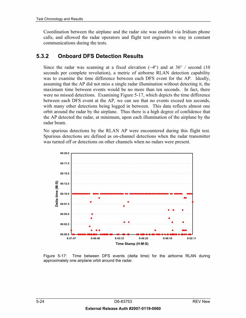
Test Chronology and Results
Coordination between the airplane and the radar site was enabled via Iridium phone calls, and allowed the radar operators and flight test engineers to stay in constant communications during the tests.
5.3.2 Onboard DFS Detection Results
Since the radar was scanning at a fixed elevation (~4°) and at 36° / second (10 seconds per complete revolution), a metric of airborne RLAN detection capability was to examine the time difference between each DFS event for the AP. Ideally, assuming that the AP did not miss a single radar illumination without detecting it, the maximum time between events would be no more than ten seconds. In fact, there were no missed detections. Examining Figure 5-17, which depicts the time difference between each DFS event at the AP, we can see that no events exceed ten seconds, with many other detections being logged in between. This data reflects almost one orbit around the radar by the airplane. Thus there is a high degree of confidence that the AP detected the radar, at minimum, upon each illumination of the airplane by the radar beam.
No spurious detections by the RLAN AP were encountered during this flight test. Spurious detections are defined as on-channel detections when the radar transmitter was turned off or detections on other channels when no radars were present.
00:00.0
00:02.5
00:05.0
00:07.5
00:10.0
00:12.5
00:15.0
00:17.5
00:20.0
9:37:47 9:40:40 9:43:33 9:46:25 9:49:18 9:52:11
Time Stamp (H:M:S)
Del
ta ti
me
(M:S
)
Figure 5-17: Time between DFS events (delta time) for the airborne RLAN during approximately one airplane orbit around the radar.
5-24 D6-83753 REV New
External Release Auth #2007-0119-0060

Test Chronology and Results
5.3.3 Radar Interference Results
Using the special firmware for the AP, the flight test crew was able to transmit continuously on a channel overlaying the radar operating frequency. At no time was the radar able to detect any interference by the RLAN – identical to the Mt. Sicker results. In order to ensure the link budget was accurate, the airplane was equipped with a high-powered RLAN emulator, capable of generating interference with the radar when turned on.
To compare the impact of the external high-powered RLAN emulator with the internal low-powered real RLAN, the RLAN onboard the airplane was turned off and on, and the external emulator was stepped through a variety of output powers while evaluating the interference into the radar.
Referring to Figure 5-18, which depicts an unfiltered “normal” radar image at the Strathmore site, the normal ground clutter, nearby mountains, and other artifacts are visible in the radar returns.
Ground Clutter dueto nearby rocky mountains
Ground clutter due tonearby terrain in sidelobes
Speckles normally filtered out (airplanes normally are not seen)
40 km range ringsGround Clutter dueto nearby rocky mountains
Ground clutter due tonearby terrain in sidelobes
Speckles normally filtered out (airplanes normally are not seen)
40 km range rings
Figure 5-18: Typical (normal) Strathmore radar image with speckle filter turned off for flight test.
REV New D6-83753 5-25
External Release Auth #2007-0119-0060

Test Chronology and Results
In Figure 5-19, the impact of operating the external RLAN emulator at a high power level of 40dBm (10W) can be seen on the radar image. The RLAN emulator’s interference completely fills all range bins of the radar processor, leading to the radial line emanating from the radar location and extending to the horizon. Additionally the aircraft itself can be seen as a higher than usual reflectivity return in the radar image.
Aircraft is seen asa “hot” spot
RLAN signal
Aircraft is seen asa “hot” spot
RLAN signal
Figure 5-19: Radar reflectivity of the airplane with an external RLAN emulator outputting 40dBm.
5-26 D6-83753 REV New
External Release Auth #2007-0119-0060
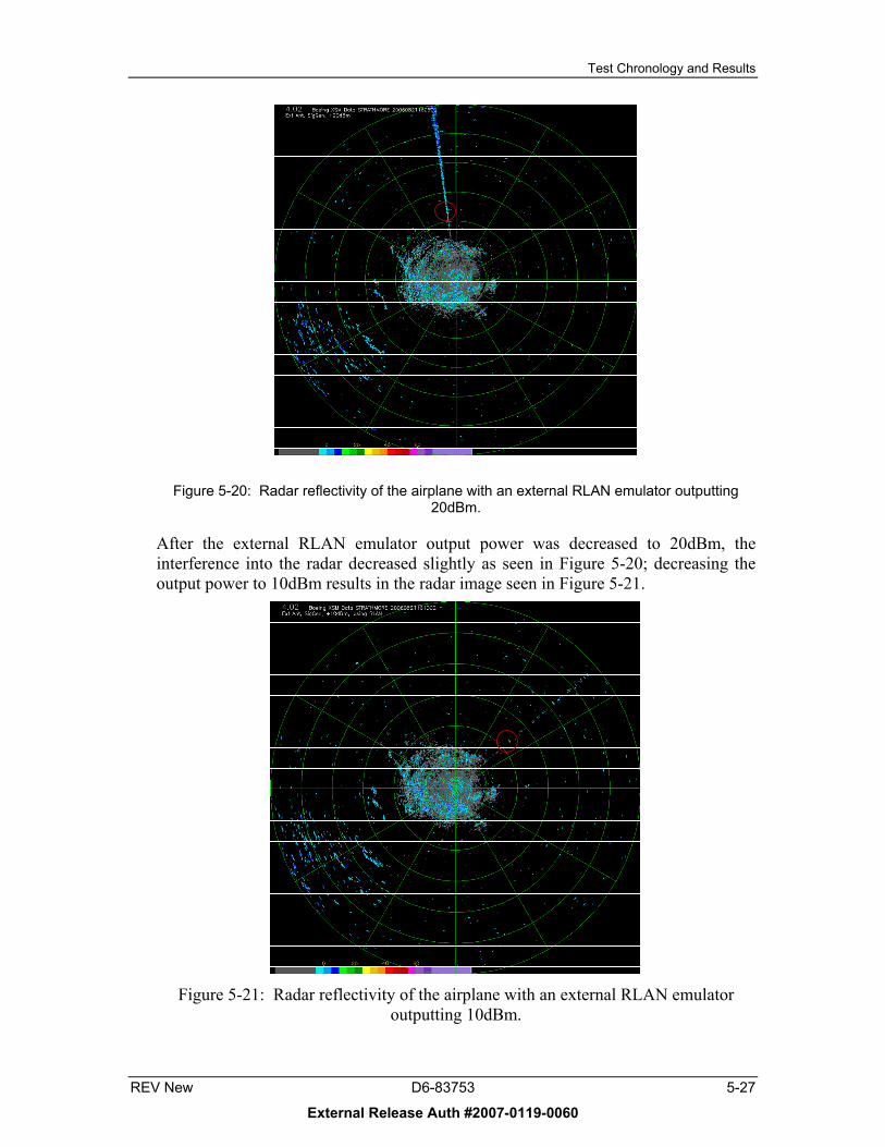
Test Chronology and Results
Figure 5-20: Radar reflectivity of the airplane with an external RLAN emulator outputting 20dBm.
After the external RLAN emulator output power was decreased to 20dBm, the interference into the radar decreased slightly as seen in Figure 5-20; decreasing the output power to 10dBm results in the radar image seen in Figure 5-21.
Figure 5-21: Radar reflectivity of the airplane with an external RLAN emulator
outputting 10dBm.
REV New D6-83753 5-27
External Release Auth #2007-0119-0060

Test Chronology and Results
The interference pattern at the radar display in Figure 5-22 is clearly breaking up, becoming less visible, and resembling the random speckle pattern seen surrounding it. At an output power of 5dBm, the external RLAN emulator was not visible on the radar display at all.
The radar image of the airplane with the internal RLAN operating is shown in Figure 5-22. As can be seen, the airplane is visible (since the speckle filter is turned off) in the image, but the streak characteristic of RLAN interference is absent, indicating that there was no interference due to the internal airborne RLAN. It’s also important to note that the RLAN was continuing to report DFS events, which normally would have triggered a channel change to avoid radar interference. Thus we can conclude that a stock (non-test specific firmware) RLAN would have correctly identified the radar and changed channels, before the radar experienced interference.
The flight test also consisted of performing an “A-B” comparison between the external emulator and the internal RLAN. In each case, the external emulator was visible, while the internal RLAN was not visible, as seen in Figure 5-22.
Aircraft locationAircraft location
Figure 5-22: Radar reflectivity of the airplane with an internal RLAN operating at 20dBm.
5-28 D6-83753 REV New
External Release Auth #2007-0119-0060

Test Chronology and Results
5.3.4 Link Budget Calculations for Strathmore
A link budget for the Strathmore flight test is shown in Figure 5-23. This budget shows the calculations for four external signal levels (40dBm, 20dBm, 10dBm, and 5dBm) and the internal RLAN signal levels as seen by terrestrial radar.
Ext 40dBm Ext 20dBm Ext 10dBm Ext 5dBm Internal RLANRLAN Tx Power (dBm/20 MHz) 40.0 20.0 10.0 5.0 20.0
Bandwidth Adjustment (WLAN to Radar) (dB) -12.0 -12.0 -12.0 -12.0 -12.0Antenna Gain (dBi) 2.0 2.0 2.0 2.0 0.0
RLAN TX Power EIRP (dBm/RadarBW) 30.0 10.0 0.0 -5.0 8.0Fuselage attenuation 0.0 0.0 0.0 0.0 -17.3
Path (free-space) loss @ 25 nm -140.7 -140.7 -140.7 -140.7 -140.7
Signal Level into Radar Antenna (dBm/RadarBW) -110.8 -130.8 -140.8 -145.8 -150.1Radar Antenna Gain (dBi) 47.5 47.5 47.5 47.5 47.5
Signal Level out of Radar Antenna (dBm/RadarBW) -63.3 -83.3 -93.3 -98.3 -102.6
Flight Test Experimental Results Stong Interference
Strong Interference
Marginal Interference No Interference No Interference
Flight Test Theoretical Link BudgetRLAN
Radar
Figure 5-23: Link budget calculations for Strathmore 25nm orbit.
The radar has a theoretical noise floor at the output of the radar antenna of approximately -110.7dBm. Noting that the two columns annotated as “no interference” are actually above the theoretical noise floor, it was suspected that the radar antenna was sub-optimally oriented to inject a maximum amount of interference noise into the radar.
Comparing the interference signal levels from the external RLAN emulator to the internal RLAN, the internal network is seen to have about 4.3dB lower noise level than 5dBm external signal (no interference detected), and 9.3dB margin with the external 10dBm signal, which has marginal impact on the radar.
However, at about 12nm (22 km), the path loss is about 9.3 dB lower and the internal RLAN signal would look like the 10 dB external antenna case and should be marginally detectable by the radar. At this latter range and for a aircraft flying at 25,000 ft (8 km), in order to see the plane, the weather radar elevation angle is about 21° above the horizon. The aircraft is approaching the cone of silence right above the radar. There is a small chance of a direct hit on the aircraft as it takes about 9 seconds to pass through the coverage area. Lower flight altitudes would increase the probability of detection due to the possibility of being scanned by the radar since the horizontal radar coverage would increase the residence time due to the ring width increases.
To determine whether the regulator requirements would have protected the radar from these signals, the AP DFS detection logs were examined for the detected radar power levels. In Figure 5-24, the detected radar power seen within the aircraft cabin is depicted. As can be seen, the radar is routinely detected.
REV New D6-83753 5-29
External Release Auth #2007-0119-0060

Test Chronology and Results
Detected Radar Power
-100
-90
-80
-70
-60
-50
-40
-30
9:38
:00
9:39
:00
9:40
:00
9:41
:00
9:42
:00
9:43
:00
9:44
:00
9:45
:00
9:46
:00
9:47
:00
9:48
:00
9:49
:00
9:50
:00
9:51
:00
9:52
:00
Time (H:M:S)
Det
ecte
d Po
wer
(dB
m)
FCC -62dBm Threshold
Figure 5-24: Radar signal power levels detected by DFS algorithm during 25nm circular orbit. Dashed vertical grid lines represent the 10-second period which the radar should have been detected.
Results from the orbit at 50nm were consistent with and similar to the closer 25nm orbit results. In this case, the radar antenna was fixed at approximately 2° elevation, with no other changes to the test protocol. The AP correctly identified the radar, and the radar encountered no interference from the onboard RLAN.
5.3.5 Conclusions from Strathmore Flight Test
With refined radar scan strategies and improved test flight patterns, more data (and better data) was obtained concerning the impact of airborne RLANs upon terrestrial weather radars. These results completely validated the results from the Mt. Sicker flight tests, which showed that:
• The DFS algorithm functions as designed in high-speed mobile platforms, correctly detecting at-risk radars
• The DFS algorithm in airborne RLAN systems detects a radar reliably upon direct illumination, and often at other times as well
• The RLAN will not interfere with weather radar at minimal slant ranges, and the radar detection algorithm will detect the radar prior to interference becoming an issue, including non-direct incidence detections at short ranges.
5-30 D6-83753 REV New
External Release Auth #2007-0119-0060

Conclusions
6. Conclusions Ground and airborne interference testing between a terrestrial weather radar and a Colubris AP with DFS was conducted in the 5GHz spectrum. Two airborne tests and one ground test was conducted. The main objective was to determine if a DFS on a high speed mobile aircraft would detect a weather radar, since existing regulations and mitigation algorithms were conceived and developed for fixed APs and weather radars.
The results from this series of flight and ground tests are clear. Using a preliminary version of the new US FCC version of the DFS algorithm in a production Colubris MAP-330 AP, tests have been performed on both airborne platforms and ground tests showing that the algorithm functions as designed.
The Colubris detection algorithm appears to be designed to maximally detect the radar regardless of the required DFS certification standards. It exceeds the certification standard in several ways, including short pulses and low PRFs.
The DFS can see the weather radar to at least to 50 km range on the ground and likely more (we performed limited range testing). In the air, the weather radar was detected by the weather radar out to a range of more than 250 km which is close to the radio horizon.
In airborne testing, a RLAN emulator operating at typical AP powers, with antennae mounted outside the fuselage could be seen at near ranges (<25 km, limited testing) by the weather radar. In the tests situations conducted, the AP’s signals were adequately attenuated by the aircraft fuselage and no interference was observed on the weather radar. An analysis indicates that at close range (less than 20 km), it is possible for the radar to see the airborne RLAN, but the aircraft is likely be in the cone of silence over the top of the weather radar where the likelihood of direct incidence is low.
Therefore, in this application, the weather radar will not experience interference.
In high bandwidth, streaming applications, the DFS is necessary to provide optimum RLAN performance even with a 5GHz “hardened” fuselage.
6.1 DFS Performance In both airborne and ground testing, the DFS algorithm functioned very well, detecting the radar signal prior to radar interference would occur, and with few spurious detections. The margin between detection and radar interference was slightly closer in ground testing, which is consistent with the design of the algorithm as pertained to a fixed RLAN with terrestrial propagation characteristics.
In airborne applications, the DFS algorithm detected the radar at increased ranges than terrestrial systems, which is unsurprising, given the free-space propagation without the additional losses of terrestrial systems. Again, the DFS algorithm detected the radar long before the radar encountered any interference.
REV New D6-83753 6-1
External Release Auth #2007-0119-0060

Conclusions
6.1.1 Limitations
While the results of this testing are extremely encouraging, it is important to highlight the limitations of this work.
• The Colubris APs have a number of attributes, which may not be present in other makes or models (unless required by law). Specifically: o The APs used for this testing seemed to be adept at detecting 0.8µs radar pulses
as they were at detecting pulses longer than 1µs, even though the FCC rules do not require such performance.
o The Colubris APs were equally adept at detecting very slow pulse trains of 4mS (250Hz PRF), which is also beyond the FCC requirements (the FCC lower limit is 700Hz PRF).
o The Colubris policy is to change channels upon detection of a radar, without regard to the ITU mandated -62dBm threshold, thus dramatically improving the link budget margin in favor of protecting the radars.
Weather radars can use pulses as short as 0.5µs, which can be very difficult to detect. This scenario was not tested during these flight tests. For a complete list of considered radar characteristics and protection, refer to [8].
6.2 Radar Interference In terrestrial testing, a production RLAN AP was able to produce a signal generating interference into the radar output. No such interference was generated by the airborne RLAN, even though the airplane flew directly over the radar at an altitude of 10,000 feet.
To validate that the flight tests were being conducted properly, an external high-powered RLAN emulator was used to generate signals, which did interfere with the weather radars. Direct A-B comparisons between the internal and external systems showed that the internal RLAN was substantially shielded by the fuselage – perhaps more than expected given prior fuselage attenuation test results.
6.3 Topics for Further Research While this work has largely answered questions concerning airborne RLANs, other mobile platforms have been less well served. The following topics are suggested as further research topics in the examination of the impact of mobile RLANs:
• An assessment of variations of radar pulse lengths, including sub-microsecond pulses • Shielding effectiveness of passenger train railcars to RLAN signals • Impact of terrestrial mobile platforms suddenly appearing in a radar scan volume.
Examples might include a train leaving a tunnel into a radar search volume, or a ship rounding a land feature, and into a search volume.
• The Colubris RLAN APs had a non-linear detection behavior and the maximum range of its ability to detect the weather radar on the ground or in the air was not
6-2 D6-83753 REV New
External Release Auth #2007-0119-0060

Conclusions
experimentally determined. Studies to determine the range performance of the DFS as compared to radar interference would be of value.
• The attenuation characteristics at 5GHz were inferred from 2GHZ studies. Additional attenuation at 5GHz is suspected which may explain why the airborne AP’s were not seen by the ground based weather radars. Additional study of fuselage attenuation characteristics over a range of frequencies of be of significant value to many industries unrelated to radar issues.
• The increase in background noise to the weather radar by a network of AP’s and vice versa was out of scope for this study. If this is a significant effect, it may have an affect on the effective noise level of the weather radar and vice versa.
• It appears that the combination of detection technology (hardware) and the detection algorithm (software) extends significant flexibility to the AP manufacturers. Consequently the DFS results reported here may not be universally applicable.
REV New D6-83753 6-3
External Release Auth #2007-0119-0060

Conclusions
6-4 D6-83753 REV New
External Release Auth #2007-0119-0060

Appendices
Appendix A: Table of EC Radar Sites
Name ID Lat (deg) Lon (deg)
Height (m)
Freq (MHz)
Ant Gain (dB)
Holyrood WTP 47.3256 -53.1286 100 5610 42.9 Marble Mtn XME 48.9297 -57.8291 556 5625 49.2 Marion Bridge XMB 45.9496 -60.2054 125 5620 42.9 Gore XGO 45.0989 -63.7033 232 5625 49.2 Chipman XNC 46.2278 -65.7000 129 5610 42.9 Val d'Irene XAM 48.4803 -67.6011 781 5630 49.2 Lac Castor WMB 48.5767 -70.6667 904 5615 42.9 Villeroy WVY 46.4496 -71.9137 120 5620 42.9 Franktown XFT 45.0408 -76.1136 144 5610 49.2 Landrienne XLA 48.5514 -77.8080 427 5625 42.9 King WKR 43.9639 -79.5742 391 5625 49.2 Britt WBI 45.7928 -80.5328 218 5635 49.2 Exeter WSO 43.3720 -81.3804 327 5610 49.2 Timmins XTI 49.2800 -81.7939 264 5620 42.9 Montreal River WGJ 47.2478 -84.5958 541 5610 42.9 Lasseter XNI 48.8547 -89.1214 509 5620 42.9 Dryden XDR 49.8582 -92.7969 442 5630 42.9 Woodlands XWL 50.1532 -97.7805 289 5625 49.2 Foxwarren XFW 50.5488 -101.0856 553 5630 42.9 Bethune XBE 50.5711 -105.1828 594 5625 49.2 Radisson XRA 52.5205 -107.4436 545 5610 42.9 Jimmy Lake WHN 54.9133 -109.9553 654 5615 42.9 Schuler XBU 50.3126 -110.1955 868 5630 42.9 Strathmore XSM 51.2062 -113.3991 983 5620 49.2 Carvel WHK 53.5603 -114.1439 762 5625 42.9 Silver Star XSS 50.3694 -119.0642 1913 5615 42.9 Spirit River WWW 55.6953 -119.2342 1049 5623 41.5 Aldergrove WUJ 49.0156 -122.4864 114 5625 42.9 Prince George XPG 53.6153 -122.9547 1131 5630 42.9 Mt Sicker XSI 48.8606 -123.7556 748 5620 49.2
REV New D6-83753 A-1
External Release Auth #2007-0119-0060


Appendices
Appendix B: EC Radar Scan Strategies Environment Canada (EC) weather radars employ a variety of volume scan strategies to produce their operational products. These scan strategies can be divided into general strategies and specific research radar scan patterns.
B.1 General Scan Strategies
B.1.1 Task name CONVOL
This task is used to collect a volume of reflectivity (rainrate) data around the radar, out to 256 km range. This task does not collect velocity or spectral width data.
• Starts at minute:second n5:00 (n=0,1,2,3,4,5) • Ray resolution: 1 degree in azimuth (~ 7 pulses averaged) • Range bin length: 1 km (8 x 125m samples averaged) • Pulse width: 2 microseconds • PRF: 250 pps (4000 microsecond PRT) • Azimuth rotation speed: 36 deg/sec • Elevation angles: 24 angles, 1 rotation at each angle, slight allowance for
elevation settling between steps, typical angles: 24.6, 21.5, 18.7, 16.3, 14.1, 12.1, 10.4, 9.0, 7.7, 6.6, 5.6, 4.8, 4.1, 3.4, 2.9, 2.4, 2.0, 1.7, 1.4, 1.1, 0.9, 0.7, 0.5, 0.3 degrees.
• Task duration: ~5 minutes
B.1.2 Task name Dopvol_1
This task collects reflectivity, radial velocity and spectral width data out to a range of 112 km. The reflectivity data is not as sensitive as in Convol, and data is collected at only three different elevation angles.
• Starts at minute:second n0:00 (n=0,1,2,3,4,5) • Ray resolution: 0.5 degree in azimuth (~120 or ~90 pulses averaged) • Range bin length: 0.5 km (1 x 500m sample) • Pulse width: 0.8 microseconds • PRF: 1190 pps ( 840 microsecond PRT) for 0.5 deg of rotation (~120 pulses)
o 892 pps (1121 microsecond PRT) for 0.5 deg of rotation (~ 90 pulses) • Azimuth rotation speed: 5 deg/sec • Elevation angles: 3 angles, 1 rotation at each angle, slight allowance for elevation
settling between steps, typical angles: 0.5, 1.5, 3.5 degrees. • Task duration: ~4 minutes
REV New D6-83753 B-1
External Release Auth #2007-0119-0060

Appendices
B.1.3 Task name Dopvol2
This task collects reflectivity, radial velocity and spectral width data out to a range of 250 km. The radial velocity and spectral data is noisier than in Dopvol1 (fewer samples are collected and less averaging is performed), but is collected out twice as far in range. The reflectivity data is not as sensitive as in Convol, and data is collected at only one elevation angle.
• Starts at minute:second n4:00 (n=0,1,2,3,4,5) • Ray resolution: 1 degree in azimuth (~80 pulses averaged) • Range bin length: 1 km (2 x 500m samples averaged) • Pulse width: 0.8 microseconds • PRF: 1190 pps ( 840 microsecond PRT) • Azimuth rotation speed: 15 deg/sec • Elevation angles: 1 angle, typical angle: 0.3 degrees. • Task duration: ~0.5 minutes
The actual start times may be a few seconds after the listed times; and most sites have their elevation angles lowered by a few tenths of a degree for operation in the winter when the cloud tops are generally lower than in the summer months.
B.2 King Site Scan Strategy
B.2.1 Task name CONVOL
• Starts at minute:second n5:00 (n=0,1,2,3,4,5) • Ray resolution: 1 degree in azimuth • Pulse width: 1.6 microseconds • PRF: 400 pps (2.5 millisecond PRT) • Azimuth rotation speed: 35 deg/sec • Elevation angles: 24 angles, 1 rotation at each angle, slight allowance for
elevation settling between steps, typical angles: 24.6, 21.5, 18.7, 16.3, 14.1, 12.1, 10.4, 9.0, 7.7, 6.6, 5.6, 4.8, 4.1, 3.4, 2.9, 2.4, 2.0, 1.7, 1.4, 1.1, 0.9, 0.7, 0.5, 0.3 degrees.
• Task duration: ~5 minutes
B.2.2 Task name Dopvol_1
• Starts at minute:second n0:00 (n=0,1,2,3,4,5) • Ray resolution: 0.5 degree in azimuth • Pulse width: 0.8 microseconds • PRF: 1190 pps ( 840 microsecond PRT) for 0.5 deg of rotation (~106 pulses)
o 892 pps (1121 microsecond PRT) for 0.5 deg of rotation (~ 80 pulses) • Azimuth rotation speed: 5.6 deg/sec
B-2 D6-83753 REV New
External Release Auth #2007-0119-0060

Appendices
• Elevation angles: 3 angles, 1 rotation at each angle, slight allowance for elevation settling between steps, typical angles: 0.5, 1.5, 3.5 degrees.
• Task duration: ~3.5 minutes
B.2.3 Task name Polppi
• Starts at minute:second n3:30 (n=0,1,2,3,4,5) • Ray resolution: 0.5 degree in azimuth • Pulse width: 0.8 microseconds • PRF: 600 pps (1666 microsecond PRT) for 0.5 deg of rotation (~50 pulses)
o 400 pps (2500 microsecond PRT) for 0.5 deg of rotation (~33 pulses) • Azimuth rotation speed: 6 deg/sec • Elevation angles: 1 angle, typical angle: 0.5 degrees. • Task duration: ~1 minute
B.2.4 Task name Dopvol2
• Starts at minute:second n4:30 (n=0,1,2,3,4,5) • Ray resolution: 1 degree in azimuth • Pulse width: 0.8 microseconds • PRF: 1190 pps ( 840 microsecond PRT) • Azimuth rotation speed: 15 deg/sec • Elevation angles: 1 angle, typical angle: 0.3 degrees. • Task duration: ~0.5 minutes
REV New D6-83753 B-3
External Release Auth #2007-0119-0060


Appendices
Appendix C: Airplane LOPA & Configuration
777-200 Layout of Passenger Arrangements (LOPA) These LOPAs describe the layout of the airplane during the flight test operations.
Partial and complete LOPA for the 777-200 airplane, partially configured as a commercial revenue plane, and with Flight Test equipment racks amidships.
Closeup LOPA of equipment test racks and AP locations.
REV New D6-83753 C-1
External Release Auth #2007-0119-0060


Appendices
Appendix D: Acronyms and Abbreviations AP Access Point CAC Channel Availability Check CIS Crew Information Services dB Decibel dBi Decibels relative to Isotropic dBm Decibels relative to a milliwatt dBZ Radar Reflectivity Factor – a decibel referent used in weather radar to
differentiate object size and mass, such as raindrops reaching the ground. DFS Dynamic Frequency Selection FAA Federal Aviation Administration FCC Federal Communication Commission HPBW Half Power Beam Width IFE In Flight Entertainment Iperf A software measuring tool for measuring TCP/UDP bandwidth in digital
networks. Monument A group of functions in a single cabinet or structure in an airplane. A Galley is
an example of a commercial aircraft monument nm Nautical Mile PRF (prf) Pulse Repetition Frequency PPS Pulses per second RFID Radio Frequency Identification RLAN Radio Local Area Network syslog an automatic logging capability common in network and computer systems
management
REV New D6-83753 D-1
External Release Auth #2007-0119-0060

Appendices
References [1] A.L. Brandão, J. Sydor, W. Brett, J. Scott, P. Joe, D. Hung, “5GHz RLAN
interference on active meteorological radars”, Proceedings IEEE VTC2005-Spring, Stockholm, Sweden, May 30-June 1, 2005.
[2] P. Joe, J. Scott, J. Sydor, A. Brandão, & A. Yongacoglu, “Radio local area network (RLAN) and C-band weather radar interference studies”, Proceedings of the 32nd AMS Radar Conference on Radar Meteorology, Albuquerque, New Mexico, Oct 24-29, 2005.
[3] Recommendation ITU-R M 1652, “Dynamic frequency selection (DFS)1 in wireless access systems including radio local area networks for the purpose of protecting the radiodetermination service in the 5 GHz band”, 2003
[4] ITU Resolution 229, “Use of the bands 5150-5 250MHz, 5250-5350MHz and 5470-5725MHz by the mobile service for the implementation of wireless access systems including radio local area networks”, 2003
[5] FCC Memorandum of Opinion and Order in the matter of Revision of Parts 2 and 15 of the Commission’s Rules to Permit Unlicensed National Information Infrastructure (U-NII) devices in the 5GHz band, ET Docket No 03-122, Jun 29, 2006.
[6] K. Kirchoff, “Analysis of expected RF attenuation from the 787 carbon fiber composite fuselage”, unpublished Boeing document, May 10, 2006. (Boeing Proprietary)
[7] Boeing Electromagnetic Effects Group, “747-400 Fuselage Attenuation of 802.11a Signals”, Boeing document number D521U140, September 17, 2004. (Boeing Proprietary)
[8] Recommendation ITU-R M.1638, “Characteristics of and protection criteria for sharing studies for radiolocation, aeronautical radionavigation and meteorological radars operating in the frequency ands between 5250 and 5850 MHz”, 2003.
Reference-1 D6-83753 REV New
External Release Auth #2007-0119-0060

Appendices
Active Page Record Page
Numbers Revision Level
Revision Type
(Added, Deleted)
Page Numbers
Revision Level
Revision Type
(Added, Deleted)
APR-1 D6-83753 REV New
External Release Auth #2007-0119-0060

Appendices
Revision Record
Revision Letter A Changes in This Revision
Type text here.
Authorization for Release
AUTHOR:
First Name MI Last Name Org. Number Date
APPROVAL:
First Name MI Last Name Org. Number Date
DOCUMENT RELEASE:
Org. Number Date
Revision Record-1 D6-83753 REV New
External Release Auth #2007-0119-0060

Appendices
REV New D6-83753 Revision Record -1
External Release Auth #2007-0119-0060
Recommended