Domain Decomposition Methods for Problems in H (curl)
by
Juan Gabriel Calvo
A dissertation submitted in partial fulfillment
of the requirements for the degree of
Doctor of Philosophy
Department of Mathematics
New York University
September 2015
Professor Olof B. Widlund

©Juan Gabriel Calvo
All rights reserved, 2015


Dedication
To my family.
iv
Acknowledgements
First, my deepest gratitude goes to my advisor Olof Widlund. I thank him
profoundly for his direction, guidance, support and advice during four years.
I would also like to thank the rest of my committee: Professors Berger, Good-
man, O’Neil and Stadler. In addition, I also thank Dr. Clark Dohrmann of the
SANDIA-Albuquerque laboratories for his help and comments throughout my re-
search.
Finally I thank my Alma Mater, Universidad de Costa Rica, for the support
during my academic education at NYU.
v

Abstract
Two domain decomposition methods for solving vector field problems posed in
H(curl) and discretized with Nedelec finite elements are considered. These finite
elements are conforming in H(curl).
A two-level overlapping Schwarz algorithm in two dimensions is analyzed, where
the subdomains are only assumed to be uniform in the sense of Peter Jones. The
coarse space is based on energy minimization and its dimension equals the number
of interior subdomain edges. Local direct solvers are based on the overlapping
subdomains. The bound for the condition number depends only on a few geometric
parameters of the decomposition. This bound is independent of jumps in the
coefficients across the interface between the subdomains for most of the different
cases considered.
A bound is also obtained for the condition number of a balancing domain de-
composition by constraints (BDDC) algorithm in two dimensions, with Jones sub-
domains. For the primal variable space, a continuity constraint for the tangential
average over each interior subdomain edge is imposed. For the averaging operator,
a new technique named deluxe scaling is used. The optimal bound is independent
of jumps in the coefficients across the interface between the subdomains.
Furthermore, a new coarse function for problems in three dimensions is intro-
duced, with only one degree of freedom per subdomain edge. In all the cases, it
is established that the algorithms are scalable. Numerical results that verify the
results are provided, including some with subdomains with fractal edges and others
obtained by a mesh partitioner.
vi

Contents
Dedication . . . . . . . . . . . . . . . . . . . . . . . . . . . . . . . . . . . iv
Acknowledgements . . . . . . . . . . . . . . . . . . . . . . . . . . . . . . v
Abstract . . . . . . . . . . . . . . . . . . . . . . . . . . . . . . . . . . . . vi
List of Figures . . . . . . . . . . . . . . . . . . . . . . . . . . . . . . . . . x
List of Tables . . . . . . . . . . . . . . . . . . . . . . . . . . . . . . . . . xii
1 Introduction 1
1.1 An overview . . . . . . . . . . . . . . . . . . . . . . . . . . . . . . . 1
1.2 Iterative methods for solving linear systems . . . . . . . . . . . . . 4
1.3 Organization of the dissertation . . . . . . . . . . . . . . . . . . . . 7
2 Finite Element spaces 9
2.1 Sobolev spaces . . . . . . . . . . . . . . . . . . . . . . . . . . . . . 9
2.2 Triangulations . . . . . . . . . . . . . . . . . . . . . . . . . . . . . . 11
2.3 Nodal finite elements . . . . . . . . . . . . . . . . . . . . . . . . . . 12
2.4 Nedelec finite elements . . . . . . . . . . . . . . . . . . . . . . . . . 13
2.4.1 Nedelec elements in two dimensions . . . . . . . . . . . . . 14
2.4.2 Nedelec elements in three dimensions . . . . . . . . . . . . . 15
2.5 An inverse inequality . . . . . . . . . . . . . . . . . . . . . . . . . . 17
vii

2.6 A discrete Helmholtz decomposition . . . . . . . . . . . . . . . . . . 18
3 A model problem 20
3.1 Introduction . . . . . . . . . . . . . . . . . . . . . . . . . . . . . . . 20
3.2 Weak form and discretization . . . . . . . . . . . . . . . . . . . . . 21
3.3 Notation . . . . . . . . . . . . . . . . . . . . . . . . . . . . . . . . . 22
3.4 Some implementation details . . . . . . . . . . . . . . . . . . . . . . 25
3.5 Some previous work on vector-valued problems . . . . . . . . . . . 27
4 John and Jones domains 29
4.1 Introduction . . . . . . . . . . . . . . . . . . . . . . . . . . . . . . . 29
4.2 Definitions and properties . . . . . . . . . . . . . . . . . . . . . . . 30
5 Domain Decomposition methods 35
5.1 Abstract Schwarz theory . . . . . . . . . . . . . . . . . . . . . . . . 35
5.1.1 Schwarz methods . . . . . . . . . . . . . . . . . . . . . . . . 35
5.1.2 Convergence theory . . . . . . . . . . . . . . . . . . . . . . . 39
5.2 Overlapping Schwarz methods . . . . . . . . . . . . . . . . . . . . . 41
5.3 BDDC methods . . . . . . . . . . . . . . . . . . . . . . . . . . . . . 43
6 An overlapping Schwarz algorithm for Nedelec vector fields in 2D 50
6.1 Introduction . . . . . . . . . . . . . . . . . . . . . . . . . . . . . . . 50
6.2 Technical tools . . . . . . . . . . . . . . . . . . . . . . . . . . . . . 51
6.2.1 Coarse functions . . . . . . . . . . . . . . . . . . . . . . . . 52
6.2.2 Cutoff functions . . . . . . . . . . . . . . . . . . . . . . . . . 52
6.2.3 Estimates for auxiliary functions . . . . . . . . . . . . . . . 55
6.3 Main result . . . . . . . . . . . . . . . . . . . . . . . . . . . . . . . 60
viii
6.3.1 The coarse space component . . . . . . . . . . . . . . . . . . 60
6.3.2 Local subspaces . . . . . . . . . . . . . . . . . . . . . . . . . 63
6.4 Numerical results . . . . . . . . . . . . . . . . . . . . . . . . . . . . 66
7 A BDDC deluxe algorithm for Nedelec vector fields in 2D 80
7.1 Introduction . . . . . . . . . . . . . . . . . . . . . . . . . . . . . . . 80
7.2 Primal constraints . . . . . . . . . . . . . . . . . . . . . . . . . . . 81
7.3 Deluxe averaging . . . . . . . . . . . . . . . . . . . . . . . . . . . . 82
7.4 Technical tools . . . . . . . . . . . . . . . . . . . . . . . . . . . . . 83
7.4.1 Convergence analysis . . . . . . . . . . . . . . . . . . . . . . 83
7.4.2 Discrete curl extensions . . . . . . . . . . . . . . . . . . . . 84
7.4.3 Estimates for auxiliary functions . . . . . . . . . . . . . . . 85
7.4.4 A stability estimate . . . . . . . . . . . . . . . . . . . . . . . 87
7.5 Condition number for the BDDC deluxe algorithm . . . . . . . . . . 94
7.6 Numerical results . . . . . . . . . . . . . . . . . . . . . . . . . . . . 96
8 An overlapping Schwarz algorithm for Nedelec vector fields in 3D 104
8.1 Introduction . . . . . . . . . . . . . . . . . . . . . . . . . . . . . . . 104
8.2 A coarse space . . . . . . . . . . . . . . . . . . . . . . . . . . . . . . 105
8.3 Numerical Results . . . . . . . . . . . . . . . . . . . . . . . . . . . . 106
Bibliography 110
ix

List of Figures
2.1 Nodal basis function for nodal elements. . . . . . . . . . . . . . . . 13
2.2 Nedelec basis function for edge elements. . . . . . . . . . . . . . . . 15
6.1 Type 1, 2, 3 and METIS subdomains . . . . . . . . . . . . . . . . . 67
6.2 Domain decomposition with Type 2 and 3 subdomains . . . . . . . 68
6.3 Domain decomposition with L-shaped subdomains . . . . . . . . . . 71
6.4 Condition number: dependence on H/δ for the two-level overlapping
Schwarz method in 2D . . . . . . . . . . . . . . . . . . . . . . . . . 72
6.5 Domain decomposition with short subdomain edges. . . . . . . . . . 72
6.6 Domain decomposition with METIS subdomains in 2D . . . . . . . 74
6.7 Condition number: dependence on the entries of B . . . . . . . . . 76
6.8 Condition number: dependence on the number of subdomains for B
not a multiple of the identity . . . . . . . . . . . . . . . . . . . . . . 77
6.9 Coefficient distribution for problems with discontinuous coefficients
inside the subdomains . . . . . . . . . . . . . . . . . . . . . . . . . 79
6.10 Coefficient distribution for problems with discontinuous coefficients
inside the subdomains and across the interface . . . . . . . . . . . . 79
7.1 Domain decomposition with Type 1 and 4 subdomains . . . . . . . 97
x
7.2 Condition number: dependence on H/h for the BDDC deluxe algo-
rithm in 2D with Type 1 and 2 subdomains . . . . . . . . . . . . . 99
7.3 Condition number: dependence on H/h for the BDDC deluxe algo-
rithm in 2D with Type 4 subdomains . . . . . . . . . . . . . . . . . 99
8.1 Domain decomposition with METIS subdomains in 3D . . . . . . . 107
xi

List of Tables
3.1 Assembling time for the stiffness matrix in 3D . . . . . . . . . . . . 27
6.1 Condition numbers and iteration counts: scalability for the two-level
overlapping Schwarz method in 2D . . . . . . . . . . . . . . . . . . 69
6.2 Condition numbers and iteration counts: dependence on H/h for
the two-level overlapping Schwarz method in 2D . . . . . . . . . . . 69
6.3 Condition numbers and iteration counts: dependence on H/δ for
the two-level overlapping Schwarz method in 2D and Type 1, 2 and
3 subdomains . . . . . . . . . . . . . . . . . . . . . . . . . . . . . . 70
6.4 Condition numbers and iteration counts: dependence on H/δ for
the two-level overlapping Schwarz method in 2D and L-shapped
subdomains . . . . . . . . . . . . . . . . . . . . . . . . . . . . . . . 70
6.5 Condition numbers and iteration counts: subdomains with small
edges for the two-level overlapping Schwarz method in 2D . . . . . 71
6.6 Condition numbers and iteration counts: discontinuous and random
coefficient distribution for the two-level overlapping Schwarz method
in 2D . . . . . . . . . . . . . . . . . . . . . . . . . . . . . . . . . . . 73
6.7 Condition numbers and iteration counts: experiments with METIS
subdomains for the two-level overlapping Schwarz method in 2D . . 74
xii
6.8 Condition numbers and iteration counts: comparison for additive,
hybrid and multiplicative Schwarz operators in 2D . . . . . . . . . . 75
6.9 Condition numbers and iteration counts: discontinuous coefficients
inside subdomains for the two-level overlapping Schwarz method in
2D . . . . . . . . . . . . . . . . . . . . . . . . . . . . . . . . . . . . 78
6.10 Condition numbers and iteration counts: discontinuous coefficients
inside subdomains and across the interface for the two-level over-
lapping Schwarz method in 2D . . . . . . . . . . . . . . . . . . . . . 78
7.1 Condition numbers and iteration counts: scalability for the BDDC
deluxe method in 2D . . . . . . . . . . . . . . . . . . . . . . . . . . 98
7.2 Condition numbers and iteration counts: dependence on H/h for
the BDDC deluxe method in 2D and Type 1 and 2 subdomains . . 100
7.3 Condition numbers and iteration counts: dependence on H/h for
the BDDC deluxe method in 2D and Type 4 subdomains . . . . . . 100
7.4 Condition numbers and iteration counts: experiments with METIS
subdomains for the BDDC deluxe method in 2D . . . . . . . . . . . 101
7.5 Condition numbers and iteration counts: discontinuous and random
coefficient distribution for the BDDC deluxe method in 2D . . . . . 102
7.6 Condition numbers and iteration counts: discontinuous coefficients
inside subdomains for the BDDC deluxe method in 2D . . . . . . . 103
7.7 Condition numbers and iteration counts: discontinuous coefficients
inside subdomains and across the interface for the BDDC deluxe
method in 2D . . . . . . . . . . . . . . . . . . . . . . . . . . . . . . 103
xiii

8.1 Condition numbers and iteration counts: scalability for the two-level
overlapping Schwarz method in 3D . . . . . . . . . . . . . . . . . . 107
8.2 Condition numbers and iteration counts: dependence on H/h for
the two-level overlapping Schwarz method in 3D . . . . . . . . . . . 108
8.3 Condition numbers and iteration counts: dependence on H/δ for
the two-level overlapping Schwarz method in 3D . . . . . . . . . . . 108
8.4 Condition numbers and iteration counts: discontinuous and random
coefficient distribution for the two-level overlapping Schwarz method
in 3D . . . . . . . . . . . . . . . . . . . . . . . . . . . . . . . . . . . 109
xiv

Chapter 1
Introduction
1.1 An overview
We are interested in solving linear systems that arise from the discretizations
of Partial Differential Equations (PDEs). There are different means to obtain an
approximate solution for a PDE numerically, such as finite elements and finite
differences, which end up with large and ill-conditioned linear systems of algebraic
equations.
Solving these linear systems is often a hard problem: direct methods require
much time and memory, and many iterative methods will converge slowly, because
of the large condition numbers of the matrices; see Section 1.2. The main goal in
this dissertation will be to construct preconditioners for such linear systems.
Domain decomposition refers to the process of subdividing the solution of a
large linear system into smaller problems whose solutions can be used to produce
a good and scalable preconditioner for the system of equations that results from
discretizing the PDE on the entire domain. They are typically used as precondi-
1
tioners for Krylov space iterative methods, such as the Conjugate Gradient (CG)
method or the Generalized Minimal Residual (GMRES) method.
These algorithms typically involve the solution of a global coarse problem (of
modest dimension) and many local subproblems. The coarse problem prevents
the condition number of the preconditioned system to grow as the number of sub-
domains increases. These resulting problems usually can be handled with exact
solvers, due to their smaller size, but inexact solvers can also be used. Geomet-
rically, a coarse grid is often used to define the coarse problem, and the original
domain is often divided into subdomains to obtain local subproblems related to
these subdomains.
The problems on the subdomains are independent, which makes domain de-
composition methods suitable for parallel computing. These algorithms can also
be used for complicated geometries. Thus, the fundamental idea of domain decom-
position methods is to reduce the solution of a problem to the solution of problems
of a similar form on parts of the domain and an easier lower-dimensional problem
on the entire domain.
There exist two main families of domain decomposition methods: overlap-
ping Schwarz methods (with overlapping subdomains) and iterative substructuring
methods (with non-overlapping subdomains).
The earliest known domain decomposition method was proposed by Hermann
A. Schwarz in 1870 as a theoretical device to deduce the existence and uniqueness of
the boundary value problem for Poisson’s equation in the union of two overlapping
subdomains, given that existence of the solution was known for the subdomains.
This method is known as the classical alternating Schwarz method; see e.g., [60]
and [13, Chapter 2.7.2]. These methods have been widely extended to different
2

problems.
With a different approach, iterative substructuring methods reduce the linear
system to a Schur complement system, by eliminating the interior unknowns of
the subdomains. Then, a preconditioner is build for this new system. Two main
classes of iterative substructuring methods are the Balancing Neumann Neumann
(BNN) type and the Finite Element Tearing and Interconnecting (FETI) type al-
gorithms; see [22, 24] respectively. There are many variants, e.g., Dual-Primal
Finite Element Tearing and Interconnecting (FETI-DP) [23], and Balancing Do-
main Decomposition by Constraints (BDDC). The latter was introduced by Clark
Dohrmann in [15], and is currently very important. Other methods, such as multi-
grid and multilevel methods, have also been considered for these problems; see e.g.
[32, 1, 33].
In this dissertation, we will mainly consider two-level overlapping Schwarz
methods and BDDC methods for solving vector-valued problems posed in H(curl)
and discretized with Nedelec finite elements, which are conforming in H(curl) and
were considered first by Jean-Claude Nedelec in [52]. The results from Chapters 6
and 7 have already appeared as technical reports [9, 10] and have been submitted
for publication.
We will use John and Jones subdomains in two dimensions, in order to obtain
a theory that applies to quite general types of subdomains; see Chapter 4. We will
also allow discontinuities across the interface in our analysis.
3

1.2 Iterative methods for solving linear systems
As already noted, there are two different approaches to solve linear systems:
direct methods, where a factorization of the matrix is fully obtained, and iterative
methods, where an approximation for the solution is obtained after a number
of iterations. Direct methods include LU decomposition (Gauss Elimination), QR
factorization, and Cholesky factorization (for symmetric positive definite matrices),
among others. For these algorithms, execution time and storage can impose serious
constraints.
Of particular importance is the nested dissection algorithm, originally proposed
by Alan George in [26], which provides a more efficient algorithm by finding an
elimination ordering, based on a divide and conquer strategy. If applied to a
k × k two-dimensional mesh, nested dissection leads to an asymptotically optimal
ordering, requiring O(n3/2) floating-point operations and O(n log n) storage (non-
zero entries in the Cholesky factorization), where n = k2 is the dimension of the
matrix. For a k × k mesh in 3D, the work is O(n2) and the storage O(n4/3), with
n = k3; see e.g., [14]. For additional pioneering work, see [46, 28, 27].
Two of the best known iterative methods are the Generalized Minimal Resid-
ual method (GMRES, [59]) and for symmetric matrices the Conjugate Gradient
method (CG, [31]). Both belong to the Krylov space methods. In this thesis, we al-
most always will use CG, since most of the matrices considered are symmetric and
positive definite, but GMRES will be used for certain non-symmetric problems,
when hybrid and multiplicative Schwarz operators are considered.
The rate of convergence of the CG method is determined by the condition
number of the linear system. Hence, we can approximate the solution in a few
iterations if the problem is very well-conditioned. If the arithmetic is exact, after
4

n iterations we obtain the exact solution but given that n is very large, the goal
is to obtain an accurate solution with just a few iterations. We present the basic
algorithm and a lemma for CG; see, e.g., [68, Chapter 38]. For a description of the
GMRES method, we refer to [59, 68].
Data: A, b, tolerance ε, initial guess u0
Result: Approximation for the solution of Au = b
Initialize r0 = b− Au0;
while ‖rk‖ > ε do
βk = (rk−1, rk−1)/(rk−2, rk−2) (β1 = 0);
pk = rk−1 + βkpk−1;
αk = (rk−1, rk−1)/(pk, Apk);
uk = uk−1 + αkpk;
rk = rk−1 − αkApk;
end
Algorithm 1: Conjugate Gradient
Lemma 1.2.1. Let A be symmetric positive definite. Then, the iterate uk of the
Conjugate Gradient method minimizes ‖uk − u‖A over the space
u0 + spanr0, Ar0, . . . , Ak−1r0,
where u is the solution of Au = b, r0 = b−A0u0 and ‖u‖A := uTAu. We have the
error bound
‖ek‖A‖e0‖A
≤ 2
(√κ2(A)− 1√κ2(A) + 1
)k
.
Proof. See [68, Th. 38.5].
Lemma 1.2.1 suggests that if the condition number of the matrix is large, the
5

convergence can be slow. We therefore will build a preconditioner and modify the
previous algorithm, and use the Preconditioned Conjugate Gradient (PCG). Given
a symmetric, positive definite matrix M , we consider the modified linear system
M−1/2AM−1/2v = M−1/2b, v = M1/2u.
We note that M−1/2AM−1/2 is symmetric and positive definite, and reduces to the
identity in case M = A. We consider M a preconditioner and apply Algorithm 1 to
this modified system to obtain the PCG; see Algorithm 2, were we have returned
to the original variables.
Data: A, b, tolerance ε, initial guess u0
Result: Approximation for the solution of Au = b
Initialize r0 = b− Au0;
while ‖rk‖ > ε do
Precondition: zk−1 = M−1rk−1;
βk = (zk−1, rk−1)/(zk−2, rk−2) (β1 = 0);
pk = zk−1 + βkpk−1;
αk = (zk−1, rk−1)/(pk, Apk);
uk = uk−1 + αkpk;
rk = rk−1 − αkApk;
end
Algorithm 2: Preconditioned Conjugate Gradient
In this case, the rate of convergence depends on the condition number of M−1A.
We also note that the algorithm additionally only involves the application of M−1.
We will focus on the construction of preconditioners, such that κ2(M−1A) is small.
This allows us to obtain a good approximation for the solution of the linear system
6
in a few iterations.
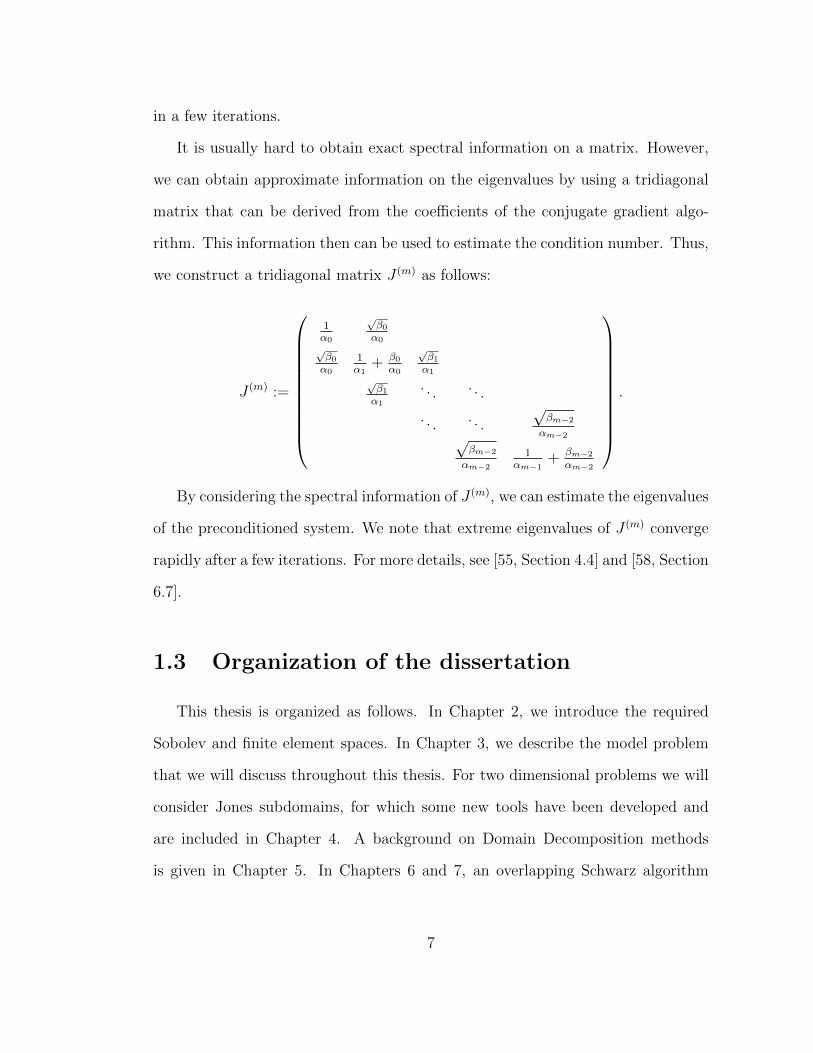
It is usually hard to obtain exact spectral information on a matrix. However,
we can obtain approximate information on the eigenvalues by using a tridiagonal
matrix that can be derived from the coefficients of the conjugate gradient algo-
rithm. This information then can be used to estimate the condition number. Thus,
we construct a tridiagonal matrix J (m) as follows:
J (m) :=
1α0
√β0
α0√β0
α0
1α1
+ β0
α0
√β1
α1√β1
α1
. . . . . .
. . . . . .√βm−2
αm−2√βm−2
αm−2
1αm−1
+ βm−2
αm−2
.
By considering the spectral information of J (m), we can estimate the eigenvalues
of the preconditioned system. We note that extreme eigenvalues of J (m) converge
rapidly after a few iterations. For more details, see [55, Section 4.4] and [58, Section
6.7].
1.3 Organization of the dissertation
This thesis is organized as follows. In Chapter 2, we introduce the required
Sobolev and finite element spaces. In Chapter 3, we describe the model problem
that we will discuss throughout this thesis. For two dimensional problems we will
consider Jones subdomains, for which some new tools have been developed and
are included in Chapter 4. A background on Domain Decomposition methods
is given in Chapter 5. In Chapters 6 and 7, an overlapping Schwarz algorithm
7
and a BDDC deluxe method are described for problems in two dimensions and
irregular subdomains, respectively. Finally, in Chapter 8, we introduce a new
coarse function for 3D problems and provide some numerical results for a two-level
overlapping Schwarz algorithm.
8

Chapter 2
Finite Element spaces
In this chapter, we introduce the Sobolev spaces and the finite element spaces
that we will use throughout our thesis. The finite element methods are based on a
variational formulation of elliptic PDEs. This variational problem has a solution in
certain function spaces called Sobolev spaces. By introducing a finite-dimensional
subspace, we discretize the equation and obtain a linear system of equations. By
solving this system, we obtain an approximate solution for the PDE.
In this study, a suitable choice for these finite element spaces are the usual
nodal Lagrange elements and the edge Nedelec elements, that will be introduced
in Sections 2.3 and 2.4. We refer to [5, 6] for general introductions to these topics.
2.1 Sobolev spaces
We consider the Sobolev space H(grad,Ω), denoted also by H1(Ω), as the
subspace of L2(Ω) with a gradient with finite L2-norm, and with a scaled norm
‖u‖2H1(Ω) := |u|2H1(Ω) +
1
H2‖u‖2
L2(Ω),
9

where H := diam(Ω), and the seminorm | · |H1(Ω) is defined by
|u|2H1(Ω) :=
∫Ω
|∇u|2 dx.
We also consider the space H(curl,Ω), the subspace of (L2(Ω))d, d = 2 or 3,
with a finite L2-norm of its curl. This is a Hilbert space with the scalar product
and graph norm defined by
(u,v)H(curl,Ω) :=
∫Ω
u · v dx +
∫Ω
∇×u · ∇ × v dx, ‖u‖2H(curl,Ω) := (u,u)H(curl,Ω).
For two dimensions, given a scalar function p and a vector u, the vector and
scalar curl operators are defined, respectively, by
∇× p :=
(∂p
∂x2
,− ∂p
∂x1
)T,
and
∇× u :=∂u2
∂x1
− ∂u1
∂x2
.
We define the unit tangent vector t on the boundary of Ω by
t := (−n2, n1)T ,
where n = (n1, n2)T is the unit outer normal vector. For a generic vector u, its
tangential component on the boundary is u · t = |n× u|.
In three dimensions, given a vector u, the curl operator is defined by
∇× u :=
(∂u3
∂x2
− ∂u2
∂x3
,∂u1
∂x3
− ∂u3
∂x1
,∂u2
∂x1
− ∂u1
∂x2
)T.
10

The tangential component of a vector u on the boundary of Ω is defined by
ut := u− (u · n)n = (n× u)× n.
Since |ut| = |n×u|, the vector u has a vanishing tangential component if and only
if n× u = 0. With an abuse of notation, we will refer to n× u as the tangential
component of u.
2.2 Triangulations
We will define finite element spaces over a triangulation of our domain in the
following sections. Given a domain Ω, we will use a triangulation Th, which is a
subdivision of Ω consisting of elements (triangles in 2D or tetrahedra in 3D). We
denote by K a generic (closed) element of the triangulation and by hK its diameter.
The following properties should hold:
1. Ω =⋃Ki
2. If Ki ∩ Kj (i 6= j) consists of one point, then it is a common vertex of Ki
and Kj.
3. If Ki∩Kj (i 6= j) consists of more than one point, then Ki∩Kj is a common
edge or face of Ki and Kj.
A family of partitions Th is called shape regular provided that there exists a
constant C > 0 such that every K ∈ Th contains a circular disk or a spherical ball
of radius ρK with ρK ≥ hK/C.
11
Finally, a family of partitions Th is called uniform provided that there exits
a constant C > 0 such that every K ∈ Th contains a circular disk or a spherical
ball of radius ρK with ρK ≥ h/C, where h := maxK hK .
2.3 Nodal finite elements
We consider the finite element spaces
W hgrad(Ω) := p ∈ C0(Ω) : p|K ∈ Pk(K),
where Pk(K) is the space of polynomials of degree k defined on a triangle or
tetrahedron K. This is a conforming space, i.e., W hgrad(Ω) ⊂ H1(Ω).
For a fixed polynomial degree k, the set of Lagrangian basis functions φhi
associated to a set of nodes Pi of the triangulation can be introduced. The basis
functions are uniquely defined by φhi (Pj) = δij, and p(x) =∑
i p(Pi)φhi (x), for
p ∈ W hgrad(Ω).
We will use linear polynomials defined over each element. The three degrees
of freedom for each triangle are the values of the function at each vertex. A nodal
function associated to a vertex in 2D is depicted in Figure 2.1.
The nodal finite element interpolant of a sufficiently smooth p ∈ H(grad,Ω) is
defined as
Ih(p) :=∑v∈Nh
p(v)φv, (2.3.1)
where N h is the set of nodes of Th, φv ∈ W hgrad(Ω) is the shape function for node
v, and p(v) is the value of p at node v. We will need the following auxiliary result:
Lemma 2.3.1. Let p be a continuous piecewise quadratic function defined on Th
12

Figure 2.1: Nodal basis function for nodal elements.
and let Ihp be its piecewise linear interpolant defined by (2.3.1) on the same mesh.
Then, there exists a constant C, depending only on the aspect ratio of K, such that
∣∣Ihp∣∣H1(K)
≤ C |p|H1(K) for K ∈ Th.
Proof. See [66, Lemma 3.9].
2.4 Nedelec finite elements
Nedelec elements are finite elements that are conforming in H(curl). Associated
with the triangulation Th, we will consider the space W hcurl(Ω) ⊂ H(curl,Ω), based
on linear triangular or tetrahedral Nedelec edge elements in Ω with zero tangential
component on ∂Ω; see [52].
13
2.4.1 Nedelec elements in two dimensions
In two dimensions with triangular elements, the restrictions to an element K
are defined by
Rk(K) := u + v : u ∈ Pk−1(K)2,v ∈ Pk(K)2,v · x = 0, k ≥ 1,
where Pk−1(K) is the space of polynomials of degree k−1 on K, Pk(K) is the space
of homogeneous polynomials of degree k on K, and a function u(x) ∈ Rk(K) is
uniquely defined by the following degrees of freedom:
∫e
u · te p ds, p ∈ Pk−1(e),
for each edge e ∈ ∂K, and, in addition, for k > 1,
∫K
u · p dx, p ∈ Pk−2(K)2.
Here te is a unit vector in the direction of e.
Those of lowest order are defined by
W hcurl(Ω) := u : u|K ∈ N1(K), K ∈ Th and u ∈ H(curl,Ω),
where any function in N1(K) has the form
u(x1, x2) = (a1 + bx2, a2 − bx1)T ,
with a1, a2, b ∈ R. The degrees of freedom for an element K ∈ Th are given by the
14
average values of the tangential component over the edges of the elements, i.e.,
λe(u) :=1
|e|
∫e
u · te ds, (2.4.1)
with e ∈ ∂K. We recall that a function in W hcurl(Ω) has a continuous tangential
component across all the fine edges; see e.g., [52]. A Nedelec function associated
to an edge in 2D is depicted in Figure 2.2.
Figure 2.2: Nedelec basis function for edge elements.
2.4.2 Nedelec elements in three dimensions
For triangulations into tetrahedra, the local spaces on a generic tetrahedron K
are defined as
Rk(K) := u + v : u ∈ Pk−1(K)3,v ∈ Pk(K)3,v · x = 0, k ≥ 1.
A vector u ∈ Rk(K) is uniquely defined by the following degrees of freedom:
15
First, for the six edges e of K,
∫e
u · te p ds, p ∈ Pk−1(e),
for k > 1 and the four faces f of K,
∫f
(u× n) · p dS, p ∈ Pk−2(f)3,
and, additionally for k > 2,
∫K
u · p dx, p ∈ Pk−3(K)3.
In the case k = 1, the elements of the local space R1(K) have the simple form
R1(K) = u = a + b× x,a, b ∈ P0(K)3.
It is immediate to see that the tangential components of a vector in R1(K) are
constant on the six edges e of K. These values, λe(u), can be taken as the degrees
of freedom, as in the two-dimensional case.
We will work with the lowest order Nedelec elements in two and three dimen-
sions. Let N e ∈ W hcurl(Ω) denote the finite element shape function for an edge e
of the finite element mesh Th. We assume that N e is scaled such that N e · te = 1
along e and N e′ · te = 0 for e 6= e′. The edge finite element interpolant of a
sufficiently smooth vector function u ∈ H(curl,Ω) is then defined as
Πh(u) :=∑e∈Mh
ueN e, ue :=1
|e|
∫e
u · teds,
16

where Mh is the set of element edges of Ω and |e| is the length of e. We will also
need the following auxiliary result:
Lemma 2.4.1. Let u ∈ W hcurl(Ω), and let θ be a continuous, piecewise linear,
scalar function on Ω. Then, there exists a constant C, depending only on the
aspect ratio of K, such that for K ∈ Th,
∥∥Πh(θu)∥∥L2(K)
≤ C ‖θu‖L2(K) ,
∥∥∇× (Πh(θu))∥∥
L2(K)≤ C ‖∇ × (θu)‖L2(K) ,
Proof. See [66, Lemma 10.8].
2.5 An inverse inequality
We present an inverse inequality for elements in the space W hcurl(Ω) which will
be used in our discussion. First, we have the following elementary estimates for a
function in W hcurl(Ω) in terms of its degrees of freedom defined in (2.4.1).
Lemma 2.5.1. Let K ∈ Th. Then, there exist positive constants c and C, depend-
ing only on the aspect ratio of K, such that for all u ∈ W hcurl(Ω), Ω ⊂ Rd,
c∑e∈∂K
hdeλ2e(u) ≤ ‖u‖2
L2(K) ≤ C∑e∈∂K
hdeλ2e(u), and
‖∇ × u‖2L2(K) ≤ C
∑e∈∂K
hd−2e λ2
e(u).
Proof. See [57, Proposition 6.3.1] or [67, Lemma 3.1] for the elementary proofs.
Combining these two inequalities, we find an inverse inequality:
17
Corollary 2.5.2 (Inverse inequality). For u ∈ W hcurl(Ω), there exists a constant
C that depends only on the aspect ratio of K, such that
‖∇ × u‖2L2(K) ≤ Ch−2
K ‖u‖2L2(K). (2.5.1)
2.6 A discrete Helmholtz decomposition
The following lemma will allow us to obtain a stable decomposition for functions
in W hcurl(Ω). The HX-preconditioner, due to Hiptmair and Xu, is based on the
following decomposition, see [34, 71].
Lemma 2.6.1. Given Ω homotopy equivalent to a ball, and u ∈ W hcurl(Ω), there
exist q ∈ W hcurl(Ω), Ψ ∈
(W h
grad(Ω))d
, p ∈ W hgrad(Ω), and a constant C, such that
u = q + Πh(Ψ) +∇p, (2.6.1)
where
‖∇p‖2L2(Ω) ≤ C
(‖u‖2
L2(Ω) +H2‖∇ × u‖2L2(Ω)
), (2.6.2a)
‖h−1q‖2L2(Ω) + ‖Ψ‖2
H1(Ω) ≤ C‖∇ × u‖2L2(Ω). (2.6.2b)
The constant C depends on Ω and the shape regularity of the mesh.
Proof. See [34, Lemma 5.1].
If the domain Ω is convex, we can improve the bounds given in (2.6.2a) and
(2.6.2b):
Lemma 2.6.2. If the domain Ω is convex, the splitting (2.6.1) from Lemma 2.6.1
18
can be chosen such that, in addition to the estimates of Lemma 2.6.1, we have
‖∇p‖2L2(Ω) ≤ C‖u‖2
L2(Ω), ‖Ψ‖2L2(Ω) ≤ C‖u‖2
L2(Ω),
with C a constant depending on the quasi-uniformity of the mesh.
Proof. See [34, Lemma 5.2].
We have also the following decomposition for John domains in two dimensions;
see Section 4 for the definition of John domains.
Lemma 2.6.3. Given a John domain D ⊂ R2 of diameter H and u ∈ W hcurl(D),
there exist p ∈ W hgrad(D), r ∈ W h
curl(D) and a constant C such that
u = ∇p+ r,
‖∇p‖2L2(D) ≤ C
(‖u‖2
L2(D) +H2‖∇ × u‖2L2(D)
), and (2.6.3a)
‖r‖2L∞(D) ≤ C
(1 + log
H
h
)‖∇ × u‖2
L2(D). (2.6.3b)
The constant C depends on D and the shape regularity of the mesh.
Proof. See [19, Lemma 3.14].
19
Chapter 3
A model problem
3.1 Introduction
The space H(curl) is used for electromagnetism and some formulations of
Navier-Stokes equations. We will consider a model problem that arises, for ex-
ample, from implicit time integration or the eddy current model of Maxwell’s
equation; see, e.g., [4, Chapter 8]. It is also considered in [2, 29, 30, 32, 34, 62, 67].
When time-dependent equations are considered, the electric field u satisfies the
equation
∇×(µ−1∇× u
)+ ε
∂2u
∂t2+ σ
∂t
∂t= −∂J
∂t, in Ω× (0, T ), (3.1.1)
where J(x, t) is the current density, and ε, µ, σ are positive definite tensors that, in
general, describe the electromagnetic properties of the medium. For their meaning
and a general discussion of Maxwell’s equations, see [51, 43, 12]. A similar equation
holds for the magnetic field. For a conducting medium and low-frequency fields,
σ is large, and the term in (3.1.1) involving the second derivative in time can be
20

neglected, giving rise to a parabolic equation.
We will consider the boundary value problem in Rd, d = 2 or 3, with a perfect
conducting boundary, given by
∇× (α∇× u) +Bu = f in Ω, (3.1.2a)
u× n = 0 on ∂Ω, (3.1.2b)
where α(x) ≥ 0, B is a d × d strictly positive definite symmetric matrix. This
PDE is obtained from (3.1.1) by a discretization in time with an implicit finite
difference time scheme, and (3.1.2) has to be solved at each time step. We could
equally well consider cases where the boundary condition (3.1.2b) is imposed only
on one or several subdomain edges or faces which form part of ∂Ω, with a natural
boundary condition over the rest of the boundary.
3.2 Weak form and discretization
In order to formulate an appropriate weak form for problem (3.1.2), we will
use the Hilbert space H(curl,Ω), see Section 2.1. By integration by parts, we then
obtain a weak formulation: Find u ∈ H0(curl,Ω) such that
a(u,v) = (f ,v) ∀ v ∈ H0(curl,Ω), (3.2.1)
with
a(u,v) :=
∫Ω
[α(∇× u) · (∇× v) +Bu · v] dx, (f ,v) :=
∫Ω
f · v dx.
(3.2.2)
21

Here, H0(curl,Ω) is the subspace of H(curl,Ω) with a vanishing tangential com-
ponent on ∂Ω.
In order to discretize equation (3.2.1), we introduce a triangulation Th as in
Section 2.2. By considering the basis N eini=1 for the finite-dimensional space
W hcurl(Ω) described in Section 2.4, we obtain the problem: Find uh ∈ W h
curl(Ω)
such that
a(uh,vh) = (f ,vh) ∀ vh ∈ W hcurl(Ω),
and the associated sparse, symmetric linear system
Au = g,
where Ai,j = a(N ej ,N ei), gi = (f ,N ei), and u is the vector of coordinates of uh
with respect to the basis N eini=1. We are interested in building preconditioners
for this ill-conditioned system of equations, given that the condition number of the
matrix A satisfies κ(A) = O(h−2).
3.3 Notation
We next introduce some notation that we will use throughout our thesis. We
will decompose the domain Ω into N non-overlapping subdomains ΩiNi=1, each of
which is the union of elements of the triangulation Th of Ω. Each Ωi will be simply
connected and will have a connected boundary ∂Ωi. We denote by Hi the diameter
of Ωi, by hi the smallest element diameter of the shape-regular triangulation Thi
of Ωi, and by H/h the maximum of the ratios Hi/hi.
In the case that we consider overlapping subdomains, we will construct Ω′i by
22
adding layers of fine elements to Ωi, and will denote by δi the minimal distance
from ∂Ω′j∩Ωi to Ωi∩Ωj, for all indices j 6= i such that Ωi∩Ω′j 6= ∅. The maximum
of the ratios Hi/δi and δi/hi are denoted by H/δ and δ/h.
The interface of the decomposition ΩiNi=1 is given by
Γ :=
(N⋃i=1
∂Ωi
)\ ∂Ω,
and the contribution to Γ from ∂Ωi by Γi := ∂Ωi \ ∂Ω. These sets are unions of
subdomain faces, edges and vertices in 3D, and subdomain edges and vertices in
2D. We recall that there are no degrees of freedom associated with the subdomain
vertices, and that the interface does not include edges and faces that lie on the
boundary of Ω. We will denote by MG the set of finite element edges on G, and
by NG the set of nodes on G.
In our analysis, we will replace B by βI, and assume that α, β are constants
αi, βi in each subdomain Ωi. We denote by ai(u,v) the bilinear form a(·, ·) defined
in (3.2.2) restricted to Ωi, and by ED(v) the energy of v over a set D, i.e.
ED(v) :=
∫D
α|∇ × v|2 + β|v|2 dx.
We can also rewrite the bilinear form (3.2.2) as
a(u,v) =N∑i=1
αi
∫Ωi
(∇× u) · (∇× v) dx + βi
∫Ωi
u · v dx.
For the 2D problems, we will denote the subdomain edges of Ωi by E ij, given
by the intersection of the closure of Ωi and Ωj, excluding the two vertices at their
endpoints. We note that the intersection of the closure of two subdomains might
23
have several components; in such a case, each component will be regarded as an
edge. We will write E instead of E ij when there is no ambiguity.
The set of all subdomain edges is defined as
SE := E ij : i < j, E ij 6= ∅
and SEi is the subset of subdomain edges which belong to Γi. When there is a
need to uniquely define the unit tangential vector tE over a subdomain edge, we
will select the subdomain with the smallest index and use the counterclockwise
direction over the boundary of the relevant subdomain. The unit vector in the
direction from one endpoint of a subdomain edge E to the other (with the same
sense of direction as tE) is denoted by dE , and the distance between the two
endpoints is dE .
Finally, we will consider subdomain edges that can be quite irregular. In two
dimensions we will consider a covering by disks of a subdomain edge, and we will
denote by χE(d)(dE/d) the number of closed circular disks of diameter d that are
required to cover it. We note that χE(d) = 1 if the edge is straight and that it can
be proved that for a prefractal Koch snowflake curve, which is a polygon with side
length hi and diameter Hi, χE(hi) ≤ (Hi/hi)log(4/3) < (Hi/hi)
1/8; see [19, Section
3.2]. This is not a large factor, being less than 10 even in the extreme case of
Hi/hi = 108.
In three dimensions, the subdomain face common to Ωi and Ωj will be denoted
by F ij, regarded as an open set, and the subdomain edges of Ωi by E ij. We
note that the intersection of the closure of two subdomains might have several
components. In such a case, each component will be regarded as a face. We will
24

write F and E instead of F ij and E ij when there is no ambiguity. The wire-basket
of the decomposition is the union of the subdomain edges, and will be denote by
W . The local contribution from Ωi to the wire-basket will be denoted by Wi.
We will also consider unit vectors tangential to ∂F and E , denoted by t∂F and
tE , respectively. The union of the closed triangles that have one edge on ∂F will
be denoted by Fb, and we then define
∆i :=⋃F∈∂Ωi
Fb.
We also define
Ξij :=(Ωi ∪ F ij ∪ Ωj
)∩(Ω′i ∩ Ω′j
), and
Υjl :=⋂m∈Ijl
Ω′m,
which is the intersection of the extensions Ω′m of all subdomains Ωm which have
the edge E jl in common with Ωi. Here, Ijl also includes i.
3.4 Some implementation details
We recall that the edge element basis functions N e satisfy
λe′(N e) =
1 if e′ = e
0 if e′ 6= e.
25
They have the representation
N e = ce (λe1∇λe2 − λe2∇λe1) , (3.4.1)
where ce is a constant independent of h such that N e · te = 1, and λe1, λe2 are the
two barycentric basis functions for the two endpoints of e.
In order to compute the entries of the matrix A, we need to evaluate the
integrals
∫K
∇×N ei · ∇ ×N ej dx and
∫K
N ei ·N ej dx, K ∈ Th.
For the linear edge elements, ∇ × N e is piecewise constant, and it is easy to
compute them from the gradient of the corresponding barycentric basis functions.
Hence, the curl-contribution for the assembled matrix is trivial. For the mass-
contribution, we use the formula
∫K
λiλj dx =1 + δijC|K|,
where δij is the usual Kronecker delta function, and C = 12 or C = 20 for two or
three dimensional problems, respectively. In order to obtain the right-hand side g,
we also use (3.4.1) with a quadrature formula.
We present in Table 3.1 the assembling time (in seconds) for the matrix A for
different values of the number of degrees of freedom and the corresponding storage
(number on non-zero entries), for the problem on the unit cube partitioned into
tetrahedral elements, with a sequential code implemented in Matlab, and a 2.4GHz
Intel Core i5 processor.
26
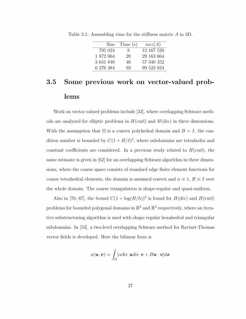
Table 3.1: Assembling time for the stiffness matrix A in 3D.
Size Time (s) nnz(A)795 024 8 12 167 520
1 872 064 20 29 163 6643 641 840 46 57 340 3526 276 384 93 99 523 824
3.5 Some previous work on vector-valued prob-
lems
Work on vector-valued problems include [33], where overlapping Schwarz meth-
ods are analyzed for elliptic problems in H(curl) and H(div) in three dimensions.
With the assumption that Ω is a convex polyhedral domain and B = I, the con-
dition number is bounded by C(1 +H/δ)2, where subdomains are tetrahedra and
constant coefficients are considered. In a previous study related to H(curl), the
same estimate is given in [62] for an overlapping Schwarz algorithm in three dimen-
sions, where the coarse space consists of standard edge finite element functions for
coarse tetrahedral elements, the domain is assumed convex and α ≡ 1, B ≡ I over
the whole domain. The coarse triangulation is shape-regular and quasi-uniform.
Also in [70, 67], the bound C(1 + log(H/h))2 is found for H(div) and H(curl)
problems for bounded polygonal domains in R3 and R2 respectively, where an itera-
tive substructuring algorithm is used with shape regular hexahedral and triangular
subdomains. In [53], a two-level overlapping Schwarz method for Raviart-Thomas
vector fields is developed. Here the bilinear form is
a(u,v) =
∫Ω
[αdiv udiv v +Bu · v]dx
27

and the condition number is bounded by C(1 +H/δ)(1 + log(H/h)), where the do-
main is a bounded polyhedron in R3 and discontinuous coefficients and hexahedral
elements are considered. A BDDC algorithm with deluxe averaging is studied in
[54] for the space H(div), with Raviart-Thomas elements, where convex polyhedral
subdomains are assumed. The condition number is bounded by C(1 + log(H/h))2,
where the constant is independent of the values and jumps of the coefficients across
the interface.
Studies based on FETI algorithms for our problem include [64, 65] for problems
posed in 2D, and [63] in 3D. The subdomains are bounded convex polyhedra and
the bounds depend on the coefficients αi, βi andHi. In addition, a BDDC algorithm
with deluxe scaling is considered in [21] for 3D.
There are also some related studies with Algebraic Multigrid Methods (AMG).
A parallel implementation of different preconditioners based on the Hiptmair-Xu
decomposition (derived in [34]) is analyzed in [40]. Also, different coarse spaces
are constructed for problems in 3D with unstructured meshes in [41]. More studies
on multigrid and multilevel methods include [32, 1, 33].
28

Chapter 4
John and Jones domains
4.1 Introduction
Previous studies on domain decomposition algorithms for our model problem
include different methods, but usually with certain restrictions such as the convex-
ity of the subdomains and the continuity of the coefficients.
As for the geometry of the substructures in two dimensions, we will consider
John domains and Jones domains; see Definitions 4.2.1 and 4.2.6. John domains
where first considered by Fritz John in work on elasticity [36], and were named
after him by Martio and Sarvas in [49]. Jones domains were introduced as (ε, δ)
domains by Peter Jones [37], and we will consider the case of δ = ∞. These
domains form the largest family of domains for which a bounded extension of
H(grad,Ω) to H(grad,R2) is possible.
In domain decomposition theory, it is typically assumed that each subdomain
is quite regular, e.g., the union of a small set of coarse triangles or tetrahedra.
But, it is unrealistic in general to assume that the subdomains are regular. Thus,
29
subdomain boundaries that arise from mesh partitioners might not even be Lips-
chitz continuous, i.e., the number of patches required to cover the boundary of the
region in each of which the boundary is the graph of a Lipschitz continuous func-
tion, might not be uniformly bounded independently of the finite element mesh
size. We also note that the shape of the subdomains are likely to change if the
mesh size is altered and a mesh partitioner is used several times.
Some recent work and technical tools have been developed for irregular subdo-
mains, cf. [69]. Scalar elliptic problems in the plane are analyzed in [16, 18]; [39]
includes a FETI-DP algorithm for scalar elliptic and elasticity problems, [17] an
overlapping Shwarz algorithm for almost incompressible elasticity, and [19] con-
cerns an iterative substructuring method, different from ours, for problems in
H(curl) in 2D. In this dissertation we will consider a two-level overlapping Schwarz
algorithm and a BDDC deluxe method for irregular subdomains in two dimensions.
4.2 Definitions and properties
We start this section by defining the type of subdomains that we will consider
for the partition of the domain of our model problem in 2D. We also collect some
well-known tools for these particular domains.
Definition 4.2.1 (John domain). A domain Ω ⊂ Rn — an open, bounded, and
connected set — is a John domain if there exists a constant CJ ≥ 1 and a dis-
tinguished central point x0 ∈ Ω, such that each x ∈ Ω can be joined to x0 by a
rectifiable curve γ : [0, 1]→ Ω, with γ(0) = x0, γ(1) = x, and
|x− γ(t)| ≤ CJ · dist (γ(t), ∂Ω) , ∀t ∈ [0, 1].
30
This condition can be viewed as a twisted cone condition. We note that certain
snowflake curves with fractal boundaries are John domains, and that the length of
the boundary of a John domain can be arbitrary much greater than its diameter.
John domains may possess internal cusps while external cusps are excluded. It is
also easy to see that diam(Ω) ≤ 2CJrΩ, where rΩ is the radius of the largest ball
inscribed in Ω and centered at x0.
Remark 4.2.2. For a rectangular domain, CJ ≥ L1/L2, where L1, L2 are the height
and width of the domain, respectively. Thus, the constant CJ can be large if the
subdomain has a large aspect ratio.
For domain decomposition methods with a coarse level, a Poincare inequality
is necessary, which is closely related to an isoperimetric inequality. We have the
following result; see [50, 25].
Lemma 4.2.3 (Isoperimetric inequality). Let Ω ⊂ Rn be a domain and let u be
sufficiently smooth. Then,
infc∈R
(∫Ω
|u− c|n/(n−1)dx
)(n−1)/n
≤ γ(Ω, n)
∫Ω
|∇u|dx, (4.2.1)
if and only if,
(min (|A|, |B|))1−1/n ≤ γ(Ω, n)|∂A ∩ ∂B|.
Here, A ⊂ Ω is an arbitrary open set, and B = Ω \ A; γ(Ω, n) is the best possible
constant and |A| is the measure of the set A, etc.
A simply connected plane domain of finite area satisfies (4.2.1) if and only if Ω
is a John domain; see [8]. Furthermore, the parameter γ(Ω, 2) can be expressed in
terms of the John constant CJ ; see [3].
31

For two dimensions, we immediately obtain a standard Poincare inequality from
(4.2.1) by using the Cauchy-Schwarz inequality. We note that the best choice of
c is uΩ, the average of u over the domain. For three dimensions, we use Holder
inequality several times.
Lemma 4.2.4 (Poincare’s inequality). Consider a John domain Ω ⊂ Rd, d = 2, 3.
Then
‖u− uΩ‖2L2(Ω) ≤ C|Ω|2/d‖∇u‖2
L2(Ω) ∀ u ∈ H(grad,Ω),
where the constant C depends on the John constant CJ(Ω).
Finally, we need the following discrete Sobolev inequality, proved in [16, Lemma
3.2] for John domains in 2D:
Lemma 4.2.5. Consider a John domain Ω ⊂ R2. For u ∈ W hgrad(Ω), there exists
a constant C such that
‖u‖2L∞(Ω) ≤ C
(1 + log
H
h
)‖u‖2
H1(Ω),
‖u− uΩ‖2L∞(Ω) ≤ C
(1 + log
H
h
)|u|2H1(Ω),
where H := diam(Ω). The constant C depends on the John constant CJ(Ω) and
the shape regularity of the elements.
We will also consider Jones domains, also known as (ε,∞) or uniform domains:
Definition 4.2.6 (Jones domain). A bounded domain Ω ⊂ R2 is uniform if there
exists a constant CU(Ω) > 0 such that for any pair of points a, b in the closure of
Ω, there is a curve γ(t) : [0, l] → Ω, parametrized by arc length, with γ(0) = a,
32
γ(l) = b, and with
l ≤ CU |a− b|,
min(|γ(t)− a|, |γ(t)− b|) ≤ CUdist(γ(t), ∂Ω).
Remark 4.2.7. The left-hand side of the second condition can be replaced by
mint
(t, l − t) or by|γ(t)− x||γ(t)− y|
|x− y|.
It is easy to see that any Jones domain is a John domain, and therefore Lemmas
4.2.4 and 4.2.5 are valid for Jones domains. The Jones domains form the largest
class of finitely connected domains for which an extension theorem holds in two
dimensions; see [37, Theorem 4].
Related to the curve γ in Definition 4.2.6, we define the following region:
Definition 4.2.8. Let a and b denote the endpoints of E = E ij ∈ SEi . The region
RE is defined as the open set with boundary ∂RE = γab∪E , where γab is the curve
γ in Definition 4.2.6.
By simple geometric considerations, it is easy to prove that RE satisfies the
following lemma; see [19, Lemma 3.4].
Lemma 4.2.9. Given a uniform subdomain Ωi and a connected subset E ⊂ ∂Ωi,
the region RE satisfies
|RE | ≤ (C2U/π)d2
E ,
diam(RE) ≤ (2CU − 1)dE .
Finally, we introduce a modified region RE related to RE , that will be used as
the support of functions constructed for each subdomain:
33

Lemma 4.2.10. Given a uniform domain Ωi and a connected subset E ⊂ ∂Ωi,
there exist a constant C, depending on CU(Ωi), and a uniform domain RE , which
is a union of finite elements of Ωi, such that RE ⊂ RE , ∂RE ∩ ∂Ωi = E, and
|RE | ≤ Cd2E ,
diam(RE) ≤ CdE .
Proof. See [19, Lemma 3.5].
34
Chapter 5
Domain Decomposition methods
Domain decomposition methods have been studied widely for different prob-
lems. We refer to [61, 56, 66] for general introductions to these topics.
5.1 Abstract Schwarz theory
We introduce the abstract Schwarz analysis in this section, which is useful in
the design and analysis of different iterative methods.
5.1.1 Schwarz methods
Consider a finite dimensional Hilbert space V . Given a symmetric, positive
definite bilinear form,
a(·, ·) : V × V → R,
and an element f ∈ V ′, we consider the problem: Find u ∈ V , such that
a(u, v) = f(v), ∀v ∈ V.
35

Given a basis for V , denote by A the corresponding stiffness matrix relative to
the bilinear form a(·, ·). Then, the problem is equivalent to the linear system
Au = f,
with A a symmetric, positive definite matrix.
We next consider a family of spaces Vi, i = 0, . . . , N, and suppose that there
exist extension operators
RTi : Vi → V.
We assume that V admits the (not necessarily a direct sum) decomposition
V = RT0 V0 +
N∑i=1
RTi Vi.
The Vi, i ≥ 1, do not need to be subspaces of V , but they are often called
subspaces or local spaces, and V0 is named the coarse space, and is usually related
to a coarse lower-dimensional problem.
We introduce local symmetric positive definite bilinear forms on the subspaces,
ai(·, ·) : Vi × Vi → R, i = 0, . . . , N,
and the associated local stiffness matrices
Ai : Vi → Vi.
36

We can use the original bilinear form on the subspaces by choosing
ai(ui, vi) = a(RTi ui, R
Ti vi), ui, vi ∈ Vi,
and then
Ai = RiARTi .
In this case, we say that we use exact local solvers.
Schwarz operators are defined in terms of projection-like operators
Pi := RTi Pi : V → RT
i Vi ⊂ V, i = 0, . . . , N,
where Pi : V → Vi is defined by
ai(Piu, vi) = a(u,RTi vi), vi ∈ Vi.
We note that Pi is well-defined since the local bilinear forms are coercive. In
the case of exact solvers, we have
a(Piu,RTi vi) = a(u,RT
i vi), vi ∈ Vi.
It can be proven easily that the Pi can be written as
Pi = RTi A−1i RiA, 0 ≤ i ≤ N,
and that in the case of exact solvers, Pi is a projection; see [66, Lemma 2.1].
We can now define a number of different Schwarz operators. The additive
37

operator is defined by
Pad :=N∑i=0
Pi. (5.1.1)
A multiplicative operator is defined by
Pmu := I − Emu, (5.1.2)
where the error propagation operator Emu is defined by
Emu := (I − PN) (I − PN−1) . . . (I − P0) .
A hybrid operator is defined by
Phy1 = I − Ehy1, Ehy1 := (I − P0)
(I −
N∑i=1
Pi
)(I − P0) , (5.1.3)
which is additive with respect to the local components and multiplicative with
respect to the levels. In the case of exact solvers, we can rewrite this operator as
Phy1 = P0 + (I − P0)N∑i=0
Pi (I − P0) .
All these Schwarz operators provide preconditioned operators for the original
operator A and can be written as the product of a suitable preconditioner and A,
where the former only involves extensions RTi , restrictions Ri, local operators A−1
i ,
and A. For example,
Pad = A−1adA, A
−1ad =
N∑i=0
RTi A−1i Ri.
38
5.1.2 Convergence theory
We consider the solution of Padu = gad, where gad := A−1ad f . In an abstract
setting, we need to consider the following assumptions:
Assumption 5.1.1. There exists a constant C0, such that every u ∈ V admits a
decomposition
u =N∑i=0
RTi ui, ui ∈ Vi, 0 ≤ i ≤ N,
that satisfiesN∑i=0
ai(ui, ui) ≤ C20a(u, u).
Assumption 5.1.2. There exist constants 0 ≤ εij ≤ 1, 1 ≤ i, j ≤ N , such that
∣∣a(RTi ui, R
Tj uj)
∣∣ ≤ εija(RTi ui, R
Ti ui)
1/2a(RTj uj, R
Tj uj)
1/2,
for ui ∈ Vi, uj ∈ Vj. We will denote the spectral radius of E = (εij) by ρ(E).
Assumption 5.1.3. There exists ω > 0 such that
a(RTi ui, R
Ti ui) ≤ ω ai(ui, ui), ui ∈ range(Pi) ⊂ Vi, 0 ≤ i ≤ N.
We then have the following lemmas:
Lemma 5.1.4. Let Assumption 5.1.1 be satisfied. Then,
a(Padu, u) ≥ C−20 a(u, u), u ∈ V.
Proof. See [66, Lemma 2.5]
39

Lemma 5.1.5. Let Assumptions 5.1.2 and 5.1.3 be satisfied. Then,
‖Pi‖a ≤ ω, for i = 0, . . . , N.
In addition,
a(Padu, u) ≤ ω (ρ(E) + 1) a(u, u).
Proof. See [66, Lemma 2.6]
Combining the previous two lemmas, we obtain the following bound for the
condition number of the preconditioned system; see [66, Theorem 2.7].
Theorem 5.1.6. The condition number of the additive Schwarz operator (5.1.1)
satisfies
κ(Pad) ≤ C20ω (ρ(E) + 1) .
Remark 5.1.7. We can bound ρ(E) by N c, the minimum number of colors needed
to color the subdomains associated with the local subproblems such that no pair of
subdomains of the same color intersect; see [66, Section 3.6]. Also, if exact solvers
are used, it is clear that ω = 1.
We also have the following bounds for the multiplicative and hybrid operators
defined in (5.1.2) and (5.1.3), respectively; see [66, Theorems 2.9 and 2.13].
Lemma 5.1.8. Let Assumptions 5.1.1, 5.1.2 and 5.1.3 be satisfied and suppose
that ω ∈ (0, 2). Then, the error propagation operator of the multiplicative Schwarz
algorithm satisfies
‖Emu‖2a ≤ 1− 2− ω
(2ω2ρ(E)2 + 1)C20
< 1,
40
where ω = max1, ω.
Lemma 5.1.9. Let Assumptions 5.1.1, 5.1.2 and 5.1.3 be satisfied, where Assump-
tion 5.1.1 holds for any u ∈ range(I− P0). Then,
max1, C20−1a(u, u) ≤ a(Phy1u, u) ≤ max1, ωρ(E)a(u, u).
5.2 Overlapping Schwarz methods
We will consider an additive two-level Schwarz algorithm for problems in 2D
and 3D in Chapters 6 and 8, respectively. The need of a coarse level arises from
the fact that the condition number estimate deteriorates as the number of subdo-
main increases. As we will see, our overlapping Schwarz methods will be scalable,
meaning that its rate of convergence does not deteriorate when the number of
subdomains grows.
We will consider a particular coarse space for each problem V0 (see Sections
6.2.1 and 8.2), and the local spaces
Vi :=wi ∈ W hi
curl(Ω′i) : wi =
∑e∈MΩ′
i
αeN e
,
where MΩ′iis the set of element edges in Ω′i, 1 ≤ i ≤ N .
We will use exact local solvers in the overlapping domains Ω′i; see Section 5.1.1.
Therefore, in order to estimate κ(Pad), our problem reduces to obtaining a constant
C20 such that
a(u0,u0) +N∑i=1
a′i(ui,ui) ≤ C20a(u,u),
41

where
u = RT0 u0 +
N∑i=1
RTi ui, u ∈ W h
curl(Ω),
and the local bilinear forms are defined by
a′i(u,u) :=
∫Ω′i
(α|∇ × u|2 + β|u|2
)dx.
By Theorem 5.1.6, the condition number of the additive operator (5.1.1) is
bounded by
κ(Pad) ≤ (NC + 1)C20 , (5.2.1)
where NC is the minimum number of colors needed to color the overlapping sub-
domains Ω′i such that no pair of subdomains of the same color intersect. Clearly,
as the overlap increases, the number of colors required can become larger.
In order to use the preconditioned conjugate gradient, we need a subroutine that
applies the preconditioner to a vector; see Algorithm 2. This is trivial if we want
to compute the action of the additive preconditioner A−1ad . For the multiplicative
preconditioner
Pmu = A−1muA,
we use the following subroutine in order to compute A−1mur. A similar subroutine
can be written for the hybrid preconditioner A−1hy1.
42
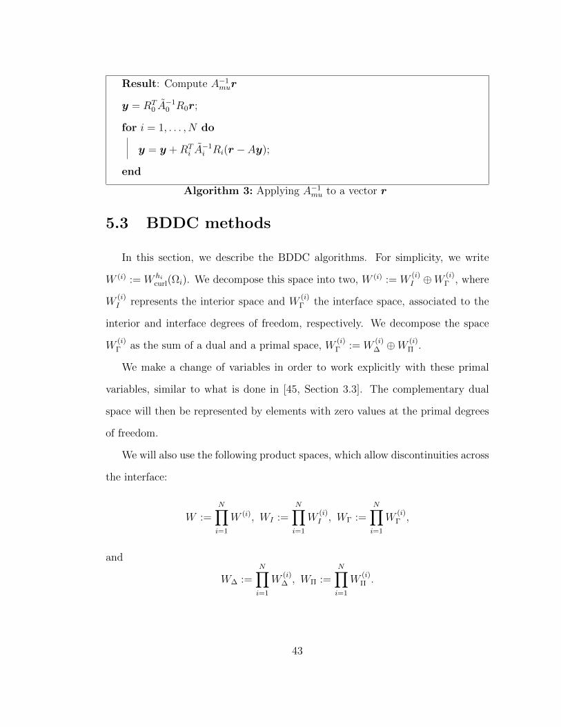
Result: Compute A−1mur
y = RT0 A−10 R0r;
for i = 1, . . . , N do
y = y +RTi A−1i Ri(r − Ay);
end
Algorithm 3: Applying A−1mu to a vector r
5.3 BDDC methods
In this section, we describe the BDDC algorithms. For simplicity, we write
W (i) := W hicurl(Ωi). We decompose this space into two, W (i) := W
(i)I ⊕W
(i)Γ , where
W(i)I represents the interior space and W
(i)Γ the interface space, associated to the
interior and interface degrees of freedom, respectively. We decompose the space
W(i)Γ as the sum of a dual and a primal space, W
(i)Γ := W
(i)∆ ⊕W
(i)Π .
We make a change of variables in order to work explicitly with these primal
variables, similar to what is done in [45, Section 3.3]. The complementary dual
space will then be represented by elements with zero values at the primal degrees
of freedom.
We will also use the following product spaces, which allow discontinuities across
the interface:
W :=N∏i=1
W (i), WI :=N∏i=1
W(i)I , WΓ :=
N∏i=1
W(i)Γ ,
and
W∆ :=N∏i=1
W(i)∆ , WΠ :=
N∏i=1
W(i)Π .
43
We then have
W = WI ⊕WΓ = WI ⊕W∆ ⊕WΠ.
The finite element solutions have a continuous tangential component across
the interface and we denote the corresponding subspace of WΓ by WΓ; generally,
functions in WΓ do not satisfy this condition. We also introduce a subspace WΓ,
intermediate between WΓ and WΓ, for which all the primal constraints are enforced.
We can then decompose
WΓ := W∆ ⊕ WΠ, WΓ := W∆ ⊕ WΠ,
where W∆ is the continuous dual variable subspace and WΠ is the continuous
primal variable subspace.
The contribution of our problem to the subdomain Ωi can be written in terms
of the local stiffness matrix A(i) and the local right hand side f (i),
A(i) =
A
(i)II A
(i)I∆ A
(i)IΠ
A(i)∆I A
(i)∆∆ A
(i)∆Π
A(i)ΠI A
(i)Π∆ A
(i)ΠΠ
, f (i) =
f
(i)I
f(i)∆
f(i)Π
. (5.3.1)
We can express the global linear system by assembling the local subdomain
problems as
A
uI
u∆
uΠ
=
AII AI∆ AIΠ
A∆I A∆∆ A∆Π
AΠI AΠ∆ AΠΠ
uI
u∆
uΠ
=
f I
f∆
fΠ
, (5.3.2)
44

with uI ∈ WI , u∆ ∈ W∆, uΠ ∈ WΠ.
We now define some operators that we will also use in our analysis. We first
introduce restriction operators. Let
R(i)Γ : WΓ → W
(i)Γ , R
(i)Γ : WΓ → W
(i)Γ
be the operators that map global interface vectors defined on Γ to their components
on Γi. Similarly, we define
R(i)∆ : W∆ → W
(i)∆ , R
(i)Π : WΠ → W
(i)Π , RΓ∆ : WΓ → W∆,
RΓΠ : WΓ → WΠ and R(i)Γ∆ : W
(i)Γ → W
(i)∆ .
We also will use the direct sums
RΓ :=N⊕i=1
R(i)Γ and RΓ :=
N⊕i=1
R(i)Γ .
Furthermore, RΓ : WΓ → WΓ will be the direct sum of RΠ and the R(i)∆ , where
RΠ : WΓ → WΠ and R(i)∆ : WΓ → W
(i)∆ are the corresponding restriction operators.
We next introduce scaling matrices D(i), acting on the degrees of freedom as-
sociated with Γi. They are combined into a block diagonal matrix and should
provide a discrete partition of unity, i.e.,
RTΓ
D(1)
D(2)
. . .
D(N)
RΓ = I. (5.3.3)
45

We then define the scaled operators R(i)D,Γ := D(i)R
(i)Γ , R
(i)D,∆ := R
(i)Γ∆R
(i)D,Γ. We
next consider a globally scaled operator RD,Γ : WΓ → WΓ defined by
RD,Γ := RΠ ⊕
(N⊕i=1
R(i)D,∆
).
From (5.3.3), it follows that
RTΓ RD,Γ = RT
D,ΓRΓ = I. (5.3.4)
Finally, we introduce an averaging operator ED : WΓ → WΓ by
ED := RΓRTD,Γ. (5.3.5)
This operator is a projection, i.e., E2D = ED; this follows from (5.3.4) and therefore
ED provides a weighted average across the interface Γ.
We will consider the subdomain Schur complements
S(i)Γ := A
(i)ΓΓ − A
(i)ΓIA
(i)−1
II A(i)IΓ, (5.3.6)
where
A(i)ΓΓ :=
A(i)∆∆ A
(i)∆Π
A(i)Π∆ A
(i)ΠΠ
is the block matrix corresponding to the interface degrees of freedom in (5.3.1).
From (5.3.6), we note that we can compute S(i)Γ times a vector by a local compu-
tation involving Ωi; the application of the inverse of A(i)II to a vector corresponds
to the solution of a Dirichlet problem in Ωi. Similarly, we can find S(i)−1
Γ u(i)Γ by
46
solving a linear system with the matrix A(i) and right hand side (0,u(i)Γ )T . Hence,
we do not need to compute the elements of the Schur complements.
We denote the global Schur complement by SΓ, given by the direct sum of
the local Schur complements S(i)Γ . By using the local Schur complements, we can
build a global interface problem. By eliminating the interior variables, the global
problem (5.3.2) can thus be reduced to
SΓuΓ = gΓ, (5.3.7)
with
SΓ :=N∑i=1
R(i)T
Γ S(i)Γ R
(i)Γ = RT
ΓSΓRΓ,
and
gΓ :=N∑i=1
R(i)T
Γ
f
(i)∆
f(i)Π
− A
(i)∆I
A(i)ΠI
A(i)−1
II f(i)I
.We will build a preconditioner for (5.3.7). Once u
(i)Γ has been found, u
(i)I is found
by solving
A(i)IIu
(i)I = f
(i)I −
(A
(i)I∆A
(i)IΠ
)u
(i)Γ .
We now consider a partially subassembled Schur complement SΓ on the space
47

WΓ: given uΓ ∈ WΓ, SΓuΓ ∈ WΓ is determined such that
A(1)II A
(1)T
∆I A(1)T
ΠI
A(1)∆I A
(1)∆∆ A
(1)T
Π∆
. . ....
A(N)II A
(N)T
∆I A(N)T
ΠI
A(N)∆I A
(N)∆∆ A
(N)T
Π∆
A(1)ΠI A
(1)Π∆ · · · A
(N)ΠI A
(N)Π∆ AΠΠ
u(1)I
u(1)∆
...
u(N)I
u(N)∆
uΠ
=
0
R(1)∆ RΓ∆SΓuΓ
...
0
R(N)∆ RΓ∆SΓuΓ
RΓΠSΓuΓ
.
Here,
AΠΠ :=N∑i=1
R(i)T
Π A(i)ΠΠR
(i)Π and Ri := R
(i)∆ RΓ∆SΓuΓ.
We note that SΓ = RT
ΓSΓRΓ, and by using restriction and extension operators,
we also find that SΓ = RTΓ SΓRΓ. Then, (5.3.7) can be rewritten as
RTΓ SΓRΓuΓ = gΓ. (5.3.8)
A linear system with the matrix SΓ can be solved by using the fact that
S−1Γ = RT
Γ∆
N∑i=1
(0 R
(i)T
∆
) A(i)II A
(i)I∆
A(i)∆I A
(i)∆∆
−1 0
R(i)∆
RΓ∆ + ΦS−1
ΠΠΦT ,
with
Φ := RTΓΠ − RT
Γ∆
N∑i=1
(0 R
(i)T
∆
) A(i)II A
(i)I∆
A(i)∆I A
(i)∆∆
−1 A
(i)T
ΠI
A(i)T
Π∆
R(i)Π
48

and where
SΠΠ :=N∑i=1
R(i)T
Π
A(i)ΠΠ −
(A
(i)ΠI A
(i)Π∆
) A(i)II A
(i)I∆
A(i)∆I A
(i)∆∆
−1 A
(i)T
ΠI
A(i)T
Π∆
R
(i)Π ;
see, e.g., [45].
In order to define a particular BDDC method, all that is left is to define the
primal constraints and the average on the interface; see Chapter 7 for the descrip-
tion of our algorithm. With these operators, we define the BDDC preconditioner
as
M−1BDDC := RT
D,ΓS−1Γ RD,Γ, (5.3.9)
and, from (5.3.8), the preconditioned linear system is given by
M−1BDDCSΓuΓ = RT
D,ΓS−1Γ RD,ΓR
TΓ SΓRΓuΓ = RT
D,ΓS−1Γ RD,ΓgΓ.
We next define norms related to the Schur complements. The SΓ-norm is
given by ‖uΓ‖2SΓ
:= uTΓSΓuΓ for uΓ ∈ WΓ. Similar expressions can be written for
‖u(i)Γ ‖2
S(i)Γ
, ‖u(i)E ‖2
S(i)E
and ‖uΓ‖2SΓ
. It is easy to see that ‖uΓ‖2SΓ
= ‖RΓuΓ‖2SΓ.
Finally, the condition number of the BDDC algorithm satisfies (see Lemmas
7.5.1 and 7.5.2):
κ(M−1BDDCSΓ) ≤ ‖ED‖2
SΓ.
49
Chapter 6
An overlapping Schwarz
algorithm for Nedelec vector
fields in 2D
6.1 Introduction
In this chapter, we analyze a two-level overlapping Schwarz method for our
problem in two dimensions, with Jones subdomains. Our study applies to a much
broader range of material properties and subdomain geometries than previous stud-
ies. We obtain the bound
κ ≤ C|Ξ|χη(
1 + logδ
h
)(1 +
H
δ
)(1 + log
H
h
),
where C is independent of the jumps of the coefficients between the subdomains.
The parameter χ is related to the geometry of the subdomains and it is quite close
50
to 1 even for fractal edges and large values of H/h (see Section 3.3), |Ξ| represents
the maximum number of neighbors for any subdomain, and
η = maxi
min
H2i
h2i
, 1 +βiH
2i
αi
,
where the maximum is taken over all the subdomains; see Section 6.3. We observe
that in many cases we can obtain a bound independent of η; see Theorem 6.3.2.
The standard way of constructing the local components involves a partition of
unity for all of Ω. This is a decomposition of functions in the sense of the Schwarz
theory as in Section 5.1. In our study, we adopt a different strategy, creating a
partition of unity for the interface and we then split the corresponding functions
supported in the different overlapping regions, in a way similar to what is done in
[17].
We also introduce a new type of cutoff function for overlapping regions with
John subdomains. We recall that certain snowflake curves with fractal boundaries
are John domains, and that the length of the boundary of a John domain can be
arbitrary greater that its diameter. This cutoff function will allow us to define
local decompositions, and can be used in different overlapping Scharwz algorithms
for problems with discontinuities in the coefficients across the interface, reducing
the problem to obtaining local bounds. This idea is used in Section 6.2.3, where
we analyze a stability result for our coarse space.
6.2 Technical tools
The auxiliary results presented in this section will be used in the proof of our
main results, Theorems 6.3.1 and 6.3.2.
51

6.2.1 Coarse functions
We will consider the same coarse space functions as introduced in [19]. For
E ∈ SE , we define the coarse function cE with tangential data given by cE ·te = dE ·te
along E and with cE · te = 0 on Γ∪∂Ω\E . We obtain cE by the energy minimizing
extension of this tangential data into the interiors of the two subdomains sharing E .
We note that the construction of cEij involves the solution of a Dirichlet problem
with inhomogeneous boundary data for Ωi and Ωj. We then define the coarse
interpolant for u ∈ H(curl,Ω) by
u0 :=∑E∈SE
uEcE , with uE :=1
dE
∫Eu · tEds. (6.2.1)
6.2.2 Cutoff functions
We introduce a new cutoff function that will provide a partition of unity on the
interface of the domain and which will be used later for the local decomposition.
The following result is valid for John subdomains.
Lemma 6.2.1. Let E ∈ SEi with endpoints a and b. Then there exists an edge
function θδE ∈ Whigrad(Ωi) that takes the value 1 at the nodes on E, vanishes in Ωi\Ω′j,
and such that
‖∇θδE‖2L2(Ωi∩Ω′j) ≤ CχE(δi)
(1 +
dEδi
)(1 + log
δihi
), (6.2.2)
for some constant C depending on CJ and the shape regularity of the elements.
Proof. For the proof of this lemma, we use similar ideas as in [18, Lemma 2.7] and
[19, Lemma 3.6]. Rename E1 := E and let E2 := ∂(Ωi ∩ Ω′j
)\ E . Split E2 into two
52

subsets, E3 := E2 ∩ ∂Ω′j and E4 := E2 \ E3. Note that E4 is a subset of ∂Ωi with two
components, one with a and the other with b as endpoints. Denote by di(x) the
distance of x to the edge Ei and consider the function θE given by
θE(x) :=1/d1(x)
1/d1(x) + 1/d2(x)
for x ∈ Ωi ∩ Ω′j and by zero everywhere else in Ωi. At the endpoints a and b,
we set this function to zero. Note that this function vanishes on E2 and takes the
required values on E . We then define θδE := Ih(θE).
We first note that the contribution from any element with a or b as an vertex
is bounded, because the gradient of the interpolant is bounded by 1/hi, since all
the nodal values are between 0 and 1.
We next estimate the energy over all the elements that do not intersect the
endpoints and lie inside Ωi ∩ Ω′j. We denote this region by R. It is easy to prove
that
|∇θE(x)| ≤ 1
d1(x) + d2(x).
We divide R into two disjoint sets, R1 := x ∈ R : d3(x) ≤ d4(x), and R2, its
complement.
First, for x ∈ R1, we note that d2(x) = d3(x). Let x1 and x3 be the points on
E1 and E3 closest to x. We have δi ≤ d(x1, E3) ≤ |x1 − x3| ≤ d1(x) + d3(x) and
then |∇θE(x)| ≤ 1/δi. As in [16, Section 4], we cover the set with square patches
with diameters of the order of δi and note that on the order of χE(δi)dE/δi of them
will suffice. The contribution of each square is bounded, and therefore
∫R1
|∇θE(x)|2dx ≤ CχE(δi)dEδi.
53

Second, for x ∈ R2, we note that d2(x) = d4(x). Denote by r(x) the minimal
distance of x to a and b. We claim that d1(x) +d4(x) ≥ Cr(x). This implies that
∫R2
|∇θE(x)|2dx ≤ C
∫R2
1
r2(x)dx ≤ C log
δihi,
by using polar coordinates centered at a and b. From the last two inequalities,
and the fact that |∇θδE | = |∇Ih(θE)| ≤ C maxx∈K |∇θE |, we obtain (6.2.2).
All that is left is to show that d1(x) + d4(x) ≥ Cr(x) for some constant C.
Without loss of generality, assume that |x−a| ≤ |x− b|. Consider the curve γ(t)
in the Definition 4.2.1 between x0 and a, and let xγ be the point on γ which is
closest to x. By the triangle inequality and the definition of a John domain, we
have that
r(x) = |x− a| ≤ |x− xγ|+ CJdist(xγ, E1).
Again by the triangle inequality and the fact that dist(xγ, E1) ≤ |xγ − x1|, where
x1 is the point on E1 closest to x, we obtain
r(x) ≤ (CJ + 1) |x− xγ|+ CJ |x− x1|.
We notice that if x lies in the region between γ and E , then |x − xγ| ≤ d4(x)
and if not, then |x − xγ| ≤ d1(x). In both cases we can deduce that |x − xγ| ≤
d1(x) + d4(x). This concludes the proof of the lemma.
From the proof of Lemma 6.2.1, we can estimate the diameter and area of
Ωi ∩ Ω′j:
54

Lemma 6.2.2. For each coarse edge E ij ∈ SEi, we have that
diam(Ωi ∩ Ω′j) ≤ CχE(δi)dE , and
|Ωi ∩ Ω′j| ≤ CχE(δi)dEδi.
Proof. Consider the covering by squares at the end of the proof of Lemma 6.2.1.
Given two points x, y ∈ Ωi ∩ Ω′j, we can join them by segments that lie in the
interior of a certain number of squares. Each of these segments have a length less
than√
2δi and since the total number of squares is on the order of χE(δi)dE/δi, we
can conclude that the diameter of Ωi ∩ Ω′j is bounded by CχE(δi)dE . The second
inequality follows by adding the area of all the squares that cover Ωi ∩ Ω′j.
6.2.3 Estimates for auxiliary functions
We start by introducing a linear interpolant for functions in W higrad(Ωi). Con-
sider an edge E ∈ SEi with endpoints a and b, and moving from a past b,
pick a point c on ∂Ωi, such that |c − b| is of order dE . Consider the function
θb` ∈ W higrad(Ωi) constructed in [18, Lemma 2.7] for the points a, b and c. This
function is uniformly bounded in Ωi, θb`(a) = 0, θb`(b) = 1, and also satisfies
‖∇θb`‖2L2(Ωi)
≤ C, and ∇θb` · te =1
dEdE · te
along E . Using this function, we introduce our linear interpolant:
Definition 6.2.3 (linear interpolant). Given f ∈ W higrad(Ωi) and a subdomain edge
55
E ∈ SEi with endpoints a and b, we define the linear function
fE`(x) := f(a) + (f(b)− f(a)) θb`(x).
We note that fE`(a) = f(a), fE`(b) = f(b), and that
∇fE`(x) · te =f(b)− f(a)
dEdE · te
along E .
Lemma 6.2.4. For any p ∈ W higrad(Ωi), there exists a function pE∆ ∈ W hi
grad(Ωi)
such that pE∆ = p− pE` along E. This function vanishes along ∂(Ωi ∩ Ω′j
)\ E and
∂Ωi \ E, and satisfies
‖∇pE∆‖2L2(Ωi)
≤ CχE(δi)
(1 + log
δihi
)(1 +
dEδi
)(1 + log
Hi
hi
)‖∇p‖2
L2(Ωi)
for some constant C depending on CJ and the shape regularity of the elements.
Proof. We define pE∆ := Ihi(θδE(p− pE`)). We use the inequality
|p(b)− p(a)|2 ≤ C
(1 + log
Hi
hi
)‖∇p‖2
L2(Ωi),
which follows from Lemma 4.2.5, and since p− pE` = (p− p(a))− (pE`− p(a)), we
have
‖p− pE`‖2L∞(Ωi∩Ω′j)
≤ C
(1 + log
Hi
hi
)‖∇p‖2
L2(Ωi).
Since ∇pE`(x) = (p(b)− p(a))∇θb`(x), we have
‖∇pE`‖2L2(Ωi∩Ω′j)
≤ C
(1 + log
Hi
hi
)‖∇p‖2
L2(Ωi).
56
From these estimates, Lemma 6.2.1 and
∇(θδE(p− pE`)) = ∇θδE(p− pE`) +∇(p− pE`)θδE ,
we find that
|θδE(p− pE`)|2H1(Ωi)≤ CχE(δi)
(1 + log
δihi
)(1 +
dEδi
)(1 + log
Hi
hi
)‖∇p‖2
L2(Ωi).
The result then follows by using Lemma 2.3.1.
Lemma 6.2.5. Given E ∈ SEi, there exists a coarse space function N E ∈ W hicurl(Ωi)
that vanishes in Ωi \Ω′j, with N E · te = dE · te along E, and N E · te = 0 everywhere
else on ∂Ωi, such that
‖N E‖2L2(Ωi)
≤ CχE(δi)dEδi,
‖∇ ×N E‖2L2(Ωi)
≤ CχE(δi)
(1 + log
δihi
)(1 +
dEδi
),
for some constant C depending on CJ and the shape regularity of the elements.
Proof. Consider the function
N E := Πhi(θδEdE) + bE/2,
where
bE := (dE · tea)N ea + (dE · teb)N eb ,
and ea, eb are the two finite element edges at the ends of E . It is easy to check
that N E matches the specified tangential data and that it vanishes in Ωi \ Ω′j.
57
By using Lemmas 2.5.1 and 2.4.1, we can prove that
‖bE‖2L2(Ωi)
≤ Ch2i , ‖∇ × bE‖2
L2(Ωi)≤ C,
‖Πhi(θδEdE)‖2L2(Ωi)
≤ CχE(δi)dEδi, and
‖∇ × Πhi(θδEdE)‖2L2(Ωi)
≤ CχE(δi)
(1 + log
δihi
)(1 +
dEδi
),
where we have also used Lemmas 6.2.1 and 6.2.2. The lemma follows by combining
these inequalities.
Lemma 6.2.6. Given r ∈ W hicurl(Ωi) and E ∈ SEi, there exists a function rE ∈
W hicurl(Ωi) that vanishes in Ωi \ Ω′j, such that rE · te = r · te along E, and with
vanishing tangential data along ∂(Ωi ∩ Ω′j) \ E and ∂Ωi \ E. Further,
‖rE‖2L2(Ωi)
≤ CχE(δi)dEδi‖r‖2L∞(Ωi∩Ω′j),
‖∇ × rE‖2L2(Ωi)
≤ C
(‖∇ × r‖2
L2(Ωi∩Ω′j)+
+ χE(δi)
(1 + log
δihi
)(1 +
dEδi
)‖r‖2
L∞(Ωi∩Ω′j)
),
for some constant C depending on CJ and the shape regularity of the elements.
Proof. We write the function r in the Nedelec basis as
r =∑
e∈MΩi
reN e,
58

and define
rE :=∑
e∈MΩi
θδ,eE reN e + (reaN ea + rebN eb) /2,
where θδ,eE is the value of θδE at the middle point of e, and ea, eb are the edges at
the ends of E . We have that
‖reaN ea + rebN eb‖2L2(Ωi)
≤ Ch2i ‖r‖2
L∞(Ωi∩Ω′j),
‖∇ × (reaN ea + rebN eb) ‖2L2(Ωi)
≤ C‖r‖2L∞(Ωi∩Ω′j),∥∥∥∥∥∥
∑e∈MΩi
θδ,eE reN e
∥∥∥∥∥∥2
L2(Ωi)
≤ C‖r‖2L2(Ωi∩Ω′j), and
∥∥∥∥∥∥∑
e∈MΩi
∇× θδ,eE reN e
∥∥∥∥∥∥2
L2(Ωi)
≤ C(‖∇ × r‖2
L2(Ωi∩Ω′j)+
+ ‖r‖2L∞(Ωi∩Ω′j)‖∇θδE‖2
L2(Ωi∩Ω′j)
).
We conclude our proof by using Lemmas 6.2.1 and 6.2.2.
Lemma 6.2.7. Given r ∈ W hicurl(Ωi), with Ωi a Jones domain, and a subdomain
edge E ∈ SEi, it holds that
|rE |2 ≤ C(‖r‖2
L∞(Ωi)+ ‖∇ × r‖2
L2(Ωi)
),
where
rE :=1
dE
∫Er · tEds (6.2.3)
and the constant C depends only on the Jones parameter CU(Ωi).
59

Proof. A similar bound is obtained in the proof of [19, Lemma 3.10] over a subset
of Ωi, from which our result follows.
6.3 Main result
6.3.1 The coarse space component
In this section, we build an explicit function that will provide a bound for the
coarse function u0 defined in (6.2.1). We consider the Helmholtz decomposition of
Lemma 2.6.3 for each uniform domain Ωi and write u = ∇pi + ri. We have
uE =pi(b)− pi(a)
dE+
1
dE
∫Eri · tE ds. (6.3.1)
For any edge E ∈ SEi , we define the function
wEi := ∇pE∆i + rEi − riEN E , (6.3.2)
where ∇pE∆i , rEi and N E are the functions from Lemmas 6.2.4, 6.2.6 and 6.2.5
respectively, and riE is given by (6.2.3). By construction, wEi vanishes in Ωi \ Ω′j.
We define wEj over Ωj ∩ Ω′i, similarly. We first find that
wEi · te = ∇pi · te + ri · te −∇pE`i · te − riEN E · te
= (u− u0) · te
along E , where we have used (6.3.1) in the last step. Similarly wEj ·te = (u−u0)·te.
60

Hence, the function wE given by
wE(x) :=
wEi (x) if x ∈ Ωi ∩ Ω′j
wEj (x) if x ∈ Ωj ∩ Ω′i
is well-defined and belongs to W hicurl(Ω), since its tangential data is continuous
across E (in fact, it is equal to the tangential component of u−u0). We note that
wE is supported in Ω′i ∩ Ω′j.
Finally, consider the function
g := u−∑E∈SE
wE . (6.3.3)
We find that g · te = u0 · te along the interface. Thus g has the same tangential
data as u0 along the interface, and therefore its energy will provide an upper bound
for the energy of u0, since u0 minimizes the energy for the specified boundary data.
We next find bounds for the energy of the components of wE . First, from
Lemma 6.2.4, (2.6.3a) and (2.5.1), we easily deduce that
ai(∇pE∆i ,∇pE∆
i ) = βi‖∇pE∆i ‖2
L2(Ωi)
≤ CχE(δi)ηi
(1 + log
δihi
)(1 +
Hi
δi
)(1 + log
Hi
hi
)ai(u,u),
(6.3.4)
where ηi := min
H2i
h2i
, 1 +βiH
2i
αi
.
61

For the second term of (6.3.2), we get from Lemma 6.2.6 and (2.6.3b),
αi‖∇ × rEi ‖2L2(Ωi)
≤ CχE(δi)
(1 + log
δihi
)(1 +
Hi
δi
)(1 + log
Hi
hi
)ai(u,u),
(6.3.5)
where we have replaced ∇× ri by ∇× u, since ∇×∇pi = 0. Also,
βi‖rEi ‖2L2(Ωi)
≤ CχE(δi)βidEδi
(1 + log
Hi
hi
)‖∇ × u‖2
L2(Ωi)
≤ CχE(δi)ηi
(1 + log
Hi
hi
)ai(u,u). (6.3.6)
From (6.3.5) and (6.3.6), we get
ai(rEi , r
Ei ) ≤ CχE(δi)ηi
(1 + log
δihi
)(1 +
Hi
δi
)(1 + log
Hi
hi
)ai(u,u). (6.3.7)
Next, from Lemmas 6.2.7 and (2.6.3b),
|riE |2 ≤ C(‖ri‖2
L∞(Ωi)+ ‖∇ × ri‖2
L2(Ωi)
)≤ C
(1 + log
Hi
hi
)‖∇ × u‖2
L2(Ωi).
62
Hence, by Lemma 6.2.5,
ai(riEN E , riEN E) = |riE |2(αi‖∇ ×N E‖2
L2(Ωi)+ βi‖N E‖2
L2(Ωi)
)≤ CχE(δi)ηi
(1 + log
δihi
)(1 +
Hi
δi
)(1 + log
Hi
hi
)ai(u,u),
(6.3.8)
by a similar argument as in (6.3.6). From (6.3.4), (6.3.7) and (6.3.8), we conclude
that
ai(wEi ,w
Ei ) ≤ CχE(δi)ηi
(1 + log
δihi
)(1 +
Hi
δi
)(1 + log
Hi
hi
)ai(u,u). (6.3.9)
From (6.3.3) and (6.3.9), we conclude that
a(u0,u0) ≤ a(g, g) ≤ C|Ξ|χη(
1 + logδ
h
)(1 +
H
δ
)(1 + log
H
h
)a(u,u),
(6.3.10)
where χ := maxi
maxE∈SEi
χE(δi), |Ξ| is the maximum number of subdomain edges for
any subdomain, and η := maxiηi. We note that ηi ≤ 2 for the curl-dominated
case, where βiH2i ≤ αi. For the mass-dominated case, where βiH
2i > αi, we cannot
always remove the factor η, but see Theorem 6.3.2 and Remark 6.3.3 for some
comments and bounds independent on η.
6.3.2 Local subspaces
For the decomposition in local components, we write
u− u0 = (u− g) + (g − u0) =∑E∈SE
wE + wr,
63

with wr := g − u0. We have that wr · te = 0 along the interface. Thus, we can
write wr =∑N
i=1 wir, with wir the restriction of wr to Ωi. We can naturally
consider a zero extension for wir to Ω′i, denoted still by wir, that satisfies
a′i(wir,wir) ≤ C|Ξ|χη(
1 + logδ
h
)(1 +
H
δ
)(1 + log
H
h
)ai(u,u). (6.3.11)
We write also ∑E∈SE
wE =N∑i=1
wEi ,
with
wEi :=1
2
∑E∈SEi
wE .
Note that wEi is supported in Ω′i and satisfies
a′i(wEi ,w
Ei ) ≤ C|Ξ|χη
(1 + log
δ
h
)(1 +
H
δ
)(1 + log
H
h
)(ai(u,u) + aj(u,u)).
(6.3.12)
Therefore, we have the decomposition
u = u0 +N∑i=1
(wir + wEi
),
and by (6.3.10), (6.3.11) and (6.3.12), we conclude that
C20 ≤ C|Ξ|χη
(1 + log
δ
h
)(1 +
H
δ
)(1 + log
H
h
). (6.3.13)
From (5.2.1) and (6.3.13), we obtain our main result:
Theorem 6.3.1. The condition number κ(Pad) of our overlapping additive two-
64

level Schwarz method is bounded by
κ(Pad) ≤ C|Ξ|χη(
1 + logδ
h
)(1 +
H
δ
)(1 + log
H
h
),
with χ = maxi
maxE∈SEi
χE(δi), η = maximin(Hi/hi)
2, 1 + βiH2i /αi, and |Ξ| is the
maximum number of subdomain edges for any subdomain. The constant C is in-
dependent of hi, Hi, δi and the coefficients αi, βi.
We can obtain a bound independent of the jumps in the coefficients across the
interface with an additional condition:
Theorem 6.3.2. If the mass-dominated subdomains are convex, then the condition
number of our overlapping additive two-level Schwarz method is bounded by
κ(Pad) ≤ C|Ξ|χ(
1 + logδ
h
)(1 +
H
δ
)(1 + log
H
h
), (6.3.14)
where C is independent of hi, Hi, δi and the coefficients αi, βi.
Proof. We can improve our result by using a stronger estimate than (2.6.3a):
‖∇p‖2L2(Ωi)
≤ C‖u‖2L2(Ωi)
; see Lemma 2.6.2. Therefore, we can simplify our es-
timate in (6.3.4) and can deduce (6.3.14).
Remark 6.3.3. Numerical experiments confirm the estimates of Theorems 6.3.1
and 6.3.2. The factor η affects the condition number only when we consider some
non-convex decompositions with mass-dominated subdomains (αi ≤ H2i βi); see
Example 6.4.3. We also note that the factor 1 + log δh
is not relevant. Numerical
results show that a small overlap gives small condition numbers for most of the
decompositions considered, with the advantage that we obtain local problems in
65
Ω′i without a significant increase in the size, compared with the local solvers over
Ωi.
6.4 Numerical results
Numerical examples are presented in this section to confirm the bound of The-
orems 6.3.1 and 6.3.2 for four different types of subdomains shown in Figure 6.1,
which have been subdivided into triangular linear edge elements. Type 1 sub-
domains have a square geometry, Type 2 subdomains include boundaries with a
“sawtooth” shape, and for Type 3 we use equilateral triangles with edges that
are part straight, part fractal. The fourth type of subdomains are obtained by
the graph partitioning software METIS [38]. Our choices of subdomain geome-
tries are similar to those of [18, Section 5]. See also [19, Section 6.1] for some
implementation details.
Some numerical results for an overlapping Schwarz method with square edge
elements are presented in [19, Section 6] without a theoretical bound. Here we
include similar experiments and have provided an analysis. We notice that our
condition numbers, in general, are smaller than those obtained in [19]. For pur-
poses of comparison, we also present results for multiplicative and hybrid Schwarz
algorithms, see Section 5.2.
For Type 1 and 2 subdomains, the ratio H/h is increased by a a factor of 2 with
each additional level of mesh refinement. At the i−th (i ≥ 0) level of refinement
for Type 3 subdomains, H/h = (H/Hf )3i+1, where H/Hf = 5 is fixed. We note
that the fractal segment lengths grow by a factor of 4/3 with each mesh refinement
whereas the straight line segments remain constant. For each refinement of Type
66

3 subdomains, every element edge on the fractal part of the boundary is first
divided into three shorter edges of 1/3 the length. The middle of these edges is
then replaced by two other edges with which it forms an equilateral triangle.
(a) Type 1 (b) Type 2
(c) Type 3 (d) Type METIS
Figure 6.1: Four types of subdomains used in the numerical examples.
We solve the resulting linear systems by using a preconditioned conjugate gra-
dient method and random right-hand sides, to a relative residual tolerance of 10−8.
The number of iterations and condition number estimates (in parenthesis) are re-
ported for each of the experiments. These estimates are obtained as mentioned in
Section 1.2.
We notice that the numerical experiments for our algorithm show an improve-
ment in the iteration count and the condition number estimates, compared to an
67

(a) Type 2 (b) Type 3
Figure 6.2: Two domain decompositions used in numerical examples for N = 16.
iterative substructuring method presented in [19]. Nevertheless, the BDDC algo-
rithm with deluxe scaling considered in the next chapter gives a further significant
improvement in the iteration counts and estimates. We note that the overlapping
Schwarz method can be used for problems for which only the fully assembled ma-
trix is available, while the BDDC and FETI methods require subdomain matrices
corresponding to subdomains problems with natural boundary conditions.
Example 6.4.1. We verify the scalability of the algorithm for Type 1 and 2
subdomains over the unit square. As shown in Table 6.1, it is clear that the
condition number is independent of the number of subdomains.
Example 6.4.2. This example is used to study the behavior of our algorithm for
increasing values of H/h. We present two experiments. First, we use Type 1, 2
and 3 subdomains with constant coefficients. Second, we consider non-constant
coefficients, arranged in a “checkerboard” pattern, using alternating values of 10−3
and 103 for βi; results are shown in Table 6.2. We note that the condition number
is not sensitive to the mesh parameter H/h.
68
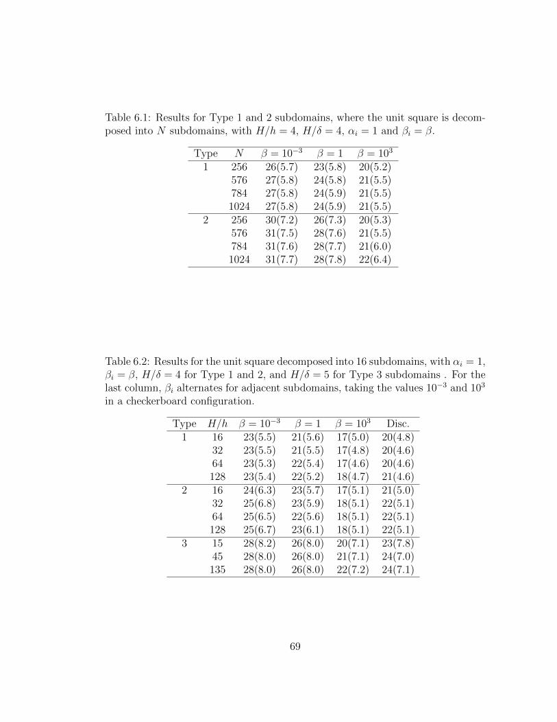
Table 6.1: Results for Type 1 and 2 subdomains, where the unit square is decom-posed into N subdomains, with H/h = 4, H/δ = 4, αi = 1 and βi = β.
Type N β = 10−3 β = 1 β = 103
1 256 26(5.7) 23(5.8) 20(5.2)576 27(5.8) 24(5.8) 21(5.5)784 27(5.8) 24(5.9) 21(5.5)1024 27(5.8) 24(5.9) 21(5.5)
2 256 30(7.2) 26(7.3) 20(5.3)576 31(7.5) 28(7.6) 21(5.5)784 31(7.6) 28(7.7) 21(6.0)1024 31(7.7) 28(7.8) 22(6.4)
Table 6.2: Results for the unit square decomposed into 16 subdomains, with αi = 1,βi = β, H/δ = 4 for Type 1 and 2, and H/δ = 5 for Type 3 subdomains . For thelast column, βi alternates for adjacent subdomains, taking the values 10−3 and 103
in a checkerboard configuration.
Type H/h β = 10−3 β = 1 β = 103 Disc.1 16 23(5.5) 21(5.6) 17(5.0) 20(4.8)
32 23(5.5) 21(5.5) 17(4.8) 20(4.6)64 23(5.3) 22(5.4) 17(4.6) 20(4.6)128 23(5.4) 22(5.2) 18(4.7) 21(4.6)
2 16 24(6.3) 23(5.7) 17(5.1) 21(5.0)32 25(6.8) 23(5.9) 18(5.1) 22(5.1)64 25(6.5) 22(5.6) 18(5.1) 22(5.1)128 25(6.7) 23(6.1) 18(5.1) 22(5.1)
3 15 28(8.2) 26(8.0) 20(7.1) 23(7.8)45 28(8.0) 26(8.0) 21(7.1) 24(7.0)135 28(8.0) 26(8.0) 22(7.2) 24(7.1)
69

Example 6.4.3. This example is used to confirm the factor (1 + H/δ) in the
condition number estimate. For Type 1 and 2 subdomains we use H/h = 100
and for Type 3 subdomains, H/h = 135, with N = 16 in all the cases. Results
are shown in Table 6.3. We notice that in these examples the growth is linear, as
expected. We also consider the decomposition shown in Figure 6.3. Results are
presented in Table 6.4. In this case, for large values of β we observe a quadratic
dependence on H/δ, but the condition numbers are in fact quite small; see Figure
6.4.
Table 6.3: Results for Type 1, 2 and 3 subdomains with 16 subdomains, αi = 1and βi = β. For Type 1 and 2 subdomains, H/h = 100; for Type 3, H/h = 135.See also Figure 6.4.
Type H/δ β = 10−3 β = 1 β = 103
1 10 30(9.8) 26(9.9) 19(5.5)20 37(17.8) 35(17.6) 22(7.9)25 40(22.6) 38(21.1) 24(8.8)50 54(40.8) 52(40.7) 30(14.6)
2 10 30(10.2) 27(10.4) 21(6.7)20 38(17.0) 34(17.1) 23(7.6)25 40(19.7) 38(19.6) 24(9.1)50 54(34.5) 49(34.1) 29(13.4)
3 15 45(33.3) 40(31.9) 26(12.1)27 56(64.7) 52(57.6) 31(20.1)45 73(121) 67(111) 37(31.0)
67.5 92(185) 81(203) 42(56.0)
Table 6.4: Results for domain decomposition shown in Figure 6.3, with 12 subdo-mains, H/h = 96, αi = 1 and βi = β. See also Figure 6.4.
H/δ β = 10−3 β = 103
24 43(23.1) 23(7.1)32 47(28.8) 24(9.0)48 58(47.0) 28(14.1)96 79(99.5) 36(39.4)
70

Figure 6.3: L-shaped domain decomposition used in Example 6.4.3. See alsoFigure 6.4 and Table 6.4.
Example 6.4.4. This example is used to confirm that the condition number esti-
mate does not require all subdomain edges to be of comparable length. Here, the
smaller subdomains shown in Figure 6.5 have only 6 elements, while the mesh pa-
rameter H/h is increased for the larger surrounding subdomains. We use N = 16
and H/δ = 4. The results are shown in Table 6.5.
Table 6.5: Results for the unit square decomposed into 16 large and 9 small sub-domains, with H/δ = 4, αi = 1, βi = β. See also Figure 6.5.
H/h β = 10−3 β = 1 β = 103
8 26(6.8) 24(7.0) 19(6.1)16 27(7.6) 25(7.0) 20(6.1)32 28(8.3) 25(7.1) 20(6.8)64 27(8.3) 25(7.0) 20(6.5)128 27(8.1) 25(7.2) 21(6.2)
71

0 20 40 60 80 1000
20
40
60
80
100
β = 10−3
β = 103
0 20 40 60 80 1000
20
40
60
β = 10−3
β = 103
0 20 40 60 80 100 120 1400
100
200
300
400
500
H/δ , Type 1, 2, 3 DD
β = 10−3
β = 103
0 10 20 30 40 500
10
20
30
40
50
60
70
β = 10−3
β = 103
0 20 40 60 80 1000
20
40
60
80
100
H/δ , METIS and L-shaped DD
β = 10−3
β = 103
Figure 6.4: Condition number as a function of H/δ. (Left) Least-squares fit to alinear polynomial in H/δ for data in Table 6.3 for β = 10−3 and β = 103. (Right)Least-squares fit to a polynomial in H/δ for a METIS and a L-shaped domaindecomposition; see data in Table 6.4.
(a) H/h = 4 (b) H/h = 8 (c) H/h = 16
Figure 6.5: Domain decomposition used in Example 6.4.4. See also Table 6.5
72
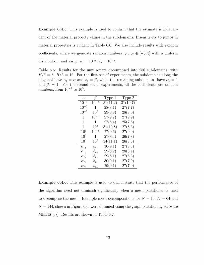
Example 6.4.5. This example is used to confirm that the estimate is indepen-
dent of the material property values in the subdomains. Insensitivity to jumps in
material properties is evident in Table 6.6. We also include results with random
coefficients, where we generate random numbers ri1, ri2 ∈ [−3, 3] with a uniform
distribution, and assign αi = 10ri1 , βi = 10ri2 .
Table 6.6: Results for the unit square decomposed into 256 subdomains, withH/δ = 8, H/h = 16. For the first set of experiments, the subdomains along thediagonal have αi = α and βi = β, while the remaining subdomains have αi = 1and βi = 1. For the second set of experiments, all the coefficients are randomnumbers, from 10−3 to 103.
α β Type 1 Type 210−3 10−3 31(11.2) 31(10.7)10−3 1 28(8.1) 27(7.7)10−3 103 29(8.8) 28(8.0)
1 10−3 27(9.7) 27(9.9)1 1 27(8.4) 25(7.8)1 103 31(10.8) 27(8.3)
103 10−3 27(9.6) 27(9.9)103 1 27(8.4) 26(7.8)103 103 34(11.1) 26(8.3)αr1 βr1 30(9.1) 27(8.3)αr2 βr2 29(8.2) 28(8.4)αr3 βr3 29(8.1) 27(8.3)αr4 βr4 30(9.1) 27(7.9)αr5 βr5 29(9.1) 27(7.9)
Example 6.4.6. This example is used to demonstrate that the performance of
the algorithm need not diminish significantly when a mesh partitioner is used
to decompose the mesh. Example mesh decompositions for N = 16, N = 64 and
N = 144, shown in Figure 6.6, were obtained using the graph partitioning software
METIS [38]. Results are shown in Table 6.7.
73

Table 6.7: Comparison of results for Type 1 subdomains and subdomains generatedby METIS. Material properties are homogeneous with αi = 1, βi = β. For Type 1subdomains, H/h = 8. For subdomains generated by METIS, see Figure 6.6.
Type N β = 10−3 β = 1 β = 103
1 16 23(5.4) 21(5.5) 16(5.0)64 24(5.6) 22(5.4) 19(4.7)
144 24(5.6) 22(5.5) 19(4.9)256 24(5.5) 23(5.5) 20(5.1)400 24(5.5) 23(5.5) 21(5.2)
METIS 16 27(7.1) 23(6.8) 19(5.3)64 33(8.8) 29(8.8) 23(5.8)
144 35(11.4) 31(10.9) 25(7.3)256 36(12.2) 31(12.0) 26(7.8)400 38(11.2) 33(11.1) 27(8.7)
(a) N = 64 (b) N = 144
Figure 6.6: Decomposition used in Example 6.4.6, obtained with the softwareMETIS.
74

Example 6.4.7. We present some results for Type 1 subdomains with the multi-
plicative and hybrid operators. We use GMRES [59] to solve the associated linear
system in the case of the non-symmetric operator Pmu. Experimental results show
that the symmetrized multiplicative Schwarz method (P symmu = I − E∗muEmu) does
not offer a significant advantage. See results in Table 6.8. The multiplicative
method improves considerably the number of iterations and the hybrid method
behaves slightly better than the additive operator.
Table 6.8: Results for Type 1 subdomains, where the unit square is decomposedinto N subdomains, with H/h = 4, H/δ = 4, αi = 1 and βi = β.
β N Pad Phy Pmu103 144 20(5.0) 18(4.5) 4
400 21(5.4) 19(5.1) 5784 21(5.5) 19(5.5) 51024 21(5.5) 19(5.6) 5
1 144 23(5.8) 22(5.3) 8400 23(5.8) 22(5.2) 9784 24(5.9) 22(5.2) 91024 24(5.9) 22(5.3) 9
10−3 144 26(5.7) 25(4.9) 12400 26(5.8) 25(4.9) 12784 27(5.8) 25(5.0) 121024 27(5.8) 25(5.0) 12
Example 6.4.8. This example is used to compare the behavior of our algorithm
when the matrix
B =
b11 b12
b12 b22
in (3.1.2) is not a constant multiple of the identity. We note that our theory does
not cover these cases, but that bounds depending on the eigenvalues of B can
be found. First we study the variation in the condition number as a function of
75

(a) b12 = 0 (b) b12 = 1
(c) b12 = 10−3 (d) b12 = 103
Figure 6.7: Condition number for different values of log b11 (x-axis) and log b22
(y-axis).
the entries of B. For this purpose, we consider Type 1 subdomains, with N = 64,
H/h = 8, H/δ = 4, α = 1; see Figure 6.7. In general, the condition number slightly
increases when there is a big difference between b11 and b22, but does not vary in
the extreme cases. We also notice a growth in the condition number as the number
of subdomains increases. Hence, in this case our coarse space is not satisfactory
and the algorithm is not scalable. Nevertheless, it only increases logarithmically,
and numerical experiments show that the condition number does not deteriorates
significantly, see Figure 6.8.
Example 6.4.9. This example is used to compare the behavior of our algorithm
76

0 500 1000 1500 2000 2500 30000
50
100
150
200
250
b11
=1
b11
=10−2
b11
=102
Figure 6.8: Condition number as a function of the number of subdomains, forType 1 subdomains with H/h = 4, H/δ = 4, α = 1, b22 = 1, b12 = b21 = 0.
when there are discontinuous coefficients inside each substructure. Each subdo-
main is divided in two subregions: in the interior we impose α = β = 1, and in the
second region the coefficients are assigned randomly as in Example 6.4.5, and then
these values are used for all the experiments; see Figure 6.9, Table 6.9 and Table
6.10. For this particular discontinuity pattern, results are similar for any set of
random numbers. We note that our theory does not cover these cases. However,
our algorithm works well even though there are discontinuities inside each subdo-
main. A second set of experiments is presented in Table 6.11. Here, each coefficient
has four different values for each quarter of the subdomain, assigned randomly for
each test; see Figure 6.10. Experimental results show that the condition number
deteriorates when we have discontinuities only for βi, as shown in Table 6.11.
77

Table 6.9: Results for the unit square decomposed into 64 subdomains, with H/δ =8 for Type 1 and 2, H/δ = 15 for Type 3, αi and βi discontinuous inside eachsubdomain, as shown in Figure 6.9, where the width of the band is 1/4 of thesubdomain diameter.
Type H/h α = 1, βi disc. β = 1, αi disc. αi, βi disc.1 16 29(9.3) 29(7.3) 30(8.4)
24 30(9.4) 29(7.4) 31(8.8)32 30(9.5) 29(7.5) 31(9.1)
2 16 29(9.2) 28(7.2) 29( 9.1)24 30(9.5) 28(7.5) 30(10.1)32 30(9.7) 29(7.7) 31(10.9)
3 15 32(21.0) 45(26.0) 30(13.2)45 33(23.0) 44(27.8) 30(14.7)135 33(24.4) 45(28.7) 32(15.1)
Table 6.10: Results for the unit square decomposed into 16 subdomains, withH/h = 48 for Type 1 and 2, H/δ = 45 for Type 3, αi and βi discontinuous insideeach subdomain, as shown in Figure 6.9, where the width of the band is 1/4 of thesubdomain diameter.
Type H/δ α = 1, βi disc. β = 1, αi disc. αi, βi disc.1 3 22(5.2) 24(5.1) 23(5.4)
6 25(6.2) 26(6.3) 27(6.9)24 37(17.7) 42(18.1) 38(16.7)
2 3 23(5.4) 24(5.4) 24(5.4)6 26(6.9) 27(6.8) 27(7.0)24 36(18.7) 40(16.1) 39(16.4)
3 5 27(8.7) 28(8.4) 25(6.4)15 32(22.7) 42(28.0) 30(14.2)
22.5 35(25.9) 52(42.2) 33(18.0)
Table 6.11: Results for the unit square decomposed into 16 Type 1 subdomains,with H/h = 16, H/δ = 8, αi and βi discontinuous inside each Ωi and on itsinterface Γi, as shown in Figure 6.10.
Test α = 1, βi disc. β = 1, αi disc. αi, βi disc.1 45(63) 35(14) 56(167)2 47(34) 34(14) 45(47)3 54(61) 35(14) 45(50)4 42(39) 36(15) 54(217)5 46(107) 34(14) 46(42)
78

−3
−2
−1
0
1
2
3
Figure 6.9: Coefficient distribution for α (left) and β (right) with Type 1 subdo-mains used in Example 6.4.9 for N = 64. The coefficients were obtained randomly,and then fixed for all the experiments. They vary from 10−3 (blue) to 103 (red).See Tables 6.9 and 6.10.
−3
−2
−1
0
1
2
3
Figure 6.10: Coefficient distribution for α (left) and β (right) with Type 1 sub-domains used in Example 6.4.9 for N = 16. The coefficients vary randomly overthe 16 subdomains, from 10−3 (blue) to 103 (red). See Table 6.11.
79
Chapter 7
A BDDC deluxe algorithm for
Nedelec vector fields in 2D
7.1 Introduction
The BDDC method was first proposed in [15] and convergence bounds for these
algorithms were provided in [47]. The BDDC methods are closely related to the
dual-primal finite element tearing and interconnecting methods (FETI-DP): the
spectra of the relevant operators of these two algorithms with the same set of
primal constraints are the same, except possibly for eigenvalues of 0 and 1; see,
e.g., [48, 45, 7].
In the construction of a BDDC preconditioner, a set of primal constraints and a
weighted average need to be chosen and these choices affect the rate of convergence.
For the primal variable space, we impose a continuity constraint for the tangential
average over each subdomain edge; see Section 7.2 for more details.
Classical choices for the weighted average include the inverse of the cardinality
80
of a subdomain edge (the number of subdomains sharing the edge) and weights
proportional to entries on the diagonals of subdomain matrices. A scaling that
depends on the coefficients α and β is considered in [63], but with the limitation
that only one coefficient is allowed to present discontinuities. We will use a deluxe
average, introduced in [20] for three dimensional problems. This technique is
used in [11], where a BDDC preconditioner is extended to Isogeometric Analysis
for scalar elliptic problems. The bound is independent of discontinuities in the
coefficients across the interface. This deluxe average is also used in [42, 54, 21].
Our study applies to a broad range of material properties and subdomain ge-
ometries. We obtain the optimal bound
κ ≤ Cχ2|Ξ|(
1 + logH
h
)2
for our deluxe BDDC method with Jones subdomains, a bound independent of the
jumps of the coefficients between the subdomains. We recall that condition number
estimates obtained in previous studies for equivalent FETI-DP methods depend
on the coefficients of the problem, and other papers include certain restrictions on
the coefficients. The constant χ is related to the geometry of the subdomains and
it is quite small even for fractal edges and large values of H/h, and |Ξ| represents
the maximum number of neighbors for any subdomain.
7.2 Primal constraints
For E ∈ SE , we define the coarse function cE similarly as in Section 6.2.1. The
primal space will be spanned by these coarse basis functions, and therefore its
dimension is the same as the number of interior subdomain edges.
81
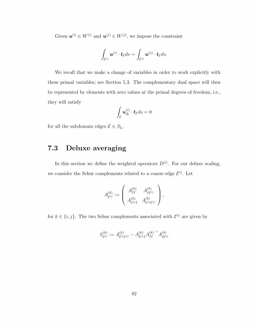
Given u(i) ∈ W (i) and u(j) ∈ W (j), we impose the constraint
∫Eij
u(i) · tEds =
∫Eij
u(j) · tEds.
We recall that we make a change of variables in order to work explicitly with
these primal variables; see Section 5.3. The complementary dual space will then
be represented by elements with zero values at the primal degrees of freedom, i.e.,
they will satisfy ∫Eu
(i)∆ · tEds = 0
for all the subdomain edges E ∈ SEi .
7.3 Deluxe averaging
In this section we define the weighted operators D(i). For our deluxe scaling,
we consider the Schur complements related to a coarse edge E ij. Let
A(k)
Eij :=
A(k)II A
(k)
IEij
A(k)
EijI A(k)
EijEij
,
for k ∈ i, j. The two Schur complements associated with E ij are given by
S(k)
Eij := A(k)
EijEij − A(k)
EijIA(k)−1
II A(k)
IEij
82

for k ∈ i, j. We define the scaling matrices D(i)j :=
(S
(i)
Eij + S(j)
Eij
)−1
S(i)
Eij . The
deluxe scaling operator D(i) is given by
D(i) :=
D(i)j1
D(i)j2
. . .
D(i)jk
where j1, . . . , jk ∈ Ξi, with Ξi the set of indices of the subdomains Ωj, j 6= i, which
share a subdomain edge with Ωi. Denote by u(i)
Eij := REiju(i) the restriction of u(i)
to the edge E ij. We can rewrite the average over E ij as
uEij =(S
(i)
Eij + S(j)
Eij
)−1 (S
(i)
Eiju(i)
Eij + S(j)
Eiju(j)
Eij
).
7.4 Technical tools
In this section, we collect some technical tools and define functions that will
be used in the proof of our main theorem.
7.4.1 Convergence analysis
Following [11, Theorem 4.4], in order to get an estimate for ‖ED‖2SΓ
, we will
reduce the problem to obtaining a bound for ‖D(j)i (u
(i)E − u
(i)ΠE)‖2
S(i)E
, where u(i)ΠE
is the primal component of u(i)Π restricted to the edge E . By using the fact that
S(i)E
(S
(i)E + S
(j)E
)−1
S(j)E is symmetric and that
S(i)E
(S
(i)E + S
(j)E
)−1
S(j)E =
(S
(i)−1
E + S(j)−1
E
)−1
< S(i)E ,
83

by simple algebra we can deduce that
‖D(j)i (u
(i)E − u
(i)ΠE)‖
2
S(i)E
+ ‖D(i)j (u
(i)E − u
(i)ΠE)‖
2
S(j)E
= (u(i)E − u
(i)ΠE)
T(S
(j)E
(S
(i)E + S
(j)E
)−1
S(i)E
(S
(i)E + S
(j)E
)−1
S(j)E +
+ S(i)E
(S
(i)E + S
(j)E
)−1
S(j)E
(S
(i)E + S
(j)E
)−1
S(i)E
)(u
(i)E − u
(i)ΠE)
= (u(i)E − u
(i)ΠE)
T(S
(i)−1
E + S(j)−1
E
)−1
(u(i)E − u
(i)ΠE)
≤ ‖u(i)E − u
(i)ΠE‖
2
S(i)E. (7.4.1)
Thus, we only need to obtain local bounds for the individual terms in the right-
hand side. For this purpose, we will construct explicit functions with the required
tangential data on E and a proper bound. This construction is presented in Section
7.4.4, where we closely follow [19, Section 4].
7.4.2 Discrete curl extensions
The space of discrete harmonic functions is directly related to the Schur com-
plements. Given u(i)Γ ∈ W
(i)Γ , we define the discrete curl extension of u
(i)Γ into Ωi
as Hi(u(i)Γ ) := u(i) where u(i) satisfies
A(i)IIu
(i)I + A
(i)IΓu
(i)Γ = 0.
Clearly Hi(u(i)Γ ) is completely defined by the tangential data on Γi. We have the
following lemma:
84

Lemma 7.4.1. The discrete curl extension u(i) = Hi(u(i)Γ ) into Ωi satisfies
ai(u(i),u(i)) = min
v(i)×n(i)=u(i)Γ
ai(v(i),v(i))
and
‖u(i)Γ ‖
2
S(i)Γ
= ai(u(i),u(i)).
Proof. The proof in [66, Lemma 4.9] for W higrad(Ωi) can be easily modified for func-
tions in W hicurl(Ωi).
7.4.3 Estimates for auxiliary functions
We borrow some results from [19], which are modifications from the technical
tools from Chapter 6, for functions now with support RE , instead of an overlap-
ping region. We start by introducing a coarse linear interpolant for functions in
W higrad(Ωi), similar to the one in Definition 6.2.3.
Definition 7.4.2 (linear interpolant). Given f ∈ W higrad(Ωi) and a subdomain edge
E ∈ SEi , we define the linear function
fE`(x) := f(a) +f(b)− f(a)
dE(x− a) · dE .
We note that fE`(a) = f(a), fE`(b) = f(b) and that fE` varies linearly in the
direction dE . We will use the following lemmas:
Lemma 7.4.3. Let RE be the uniform domain of Lemma 4.2.10. For any p ∈
W higrad(Ωi), there exists a function pE∆ ∈ W hi
grad(Ωi) such that pE∆ = p − pE` along
85

E. This function vanishes along ∂RE \ E and ∂Ωi \ E, and satisfies
‖∇pE∆‖2L2(Ωi)
≤ C
(1 + log
dEhi
)2
‖∇p‖2L2(RE)
,
for some constant C depending on CU and the shape regularity of the elements.
Proof. The proof is similar to Lemma 6.2.4, where we also need to use Lemma
4.2.10.
Lemma 7.4.4. Given r ∈ W hicurl(Ωi) and a subdomain edge E ∈ SEi, it holds that
|rE |2 ≤ C(‖r‖2
L∞(RE)+ ‖∇ × r‖2
L2(RE)
),
where
rE :=1
dE
∫Er · tEds, (7.4.2)
and the constant C depends only on the uniform parameter CU(Ωi).
Proof. This result follows from [19, Lemma 3.10] and the fact that RE ⊂ RE .
Lemma 7.4.5. Given E ∈ SEi, there exists a coarse space function N E ∈ W hicurl(Ωi)
with λe(N E) = λe(dE) along E and with λe(N E) = 0 everywhere else on ∂Ωi such
that
‖N E‖2L2(Ωi)
≤ Cd2E ,
‖∇ ×N E‖2L2(Ωi)
≤ C
(1 + log
dEhi
),
for some constant C depending on CU and the shape regularity of the elements.
Proof. The proof is similar to Lemma 6.2.5.
86

Lemma 7.4.6. Given r ∈ W hicurl(Ωi) and E ∈ SEi, there exists a function rE ∈
W hicurl(Ωi) such that λe(r
E) = λe(r) along E and with vanishing tangential data
along ∂RE \ E and ∂Ωi \ E. Further,
‖rE‖2L2(Ωi)
≤ Cd2E‖r‖2
L∞(RE),
‖∇ × rE‖2L2(Ωi)
≤ C
(‖∇ × r‖2
L2(RE)+
(1 + log
dEhi
)‖r‖2
L∞(RE)
),
for some constant C depending on CU and the shape regularity of the elements.
Proof. The proof is similar to Lemma 6.2.6.
7.4.4 A stability estimate
In this section, we will derive an edge lemma that will provide a bound for the
terms in the right-hand side of (7.4.1). For that, we split the set of edges SEi into
two subsets. We define
di := max(hi,√αi/βi
)and consider the two cases dE < di (curl-dominated) and dE ≥ di (mass-dominated)
separately. Accordingly, we partition the set of subdomain edges of Ωi as
SEi = ScEi ∪ SmEi ,
where dE < di for all the edges in ScEi , and dE ≥ di for those in SmEi . We will prove
the next lemma, using a similar construction as in [19].
87

Lemma 7.4.7. For u(i) ∈ W (i) and E ∈ SEi, there exist v(i)E ,v
(i)ΠE ∈ W (i) such that
λe(v(i)E ) = λe(u
(i)) if e ⊂ E
λe(v(i)E ) = 0 if e ⊂ ∂Ωi \ E ,
(7.4.3)
and λe(v(i)ΠE) = uEλe(dE) if e ⊂ E
λe(v(i)ΠE) = 0 if e ⊂ ∂Ωi \ E .
(7.4.4)
Furthermore,
ai(v(i)E − v
(i)ΠE ,v
(i)E − v
(i)ΠE) ≤ Cχ2
(1 + log
H
h
)2
ai(u(i),u(i)),
where χ = maxi
maxE∈Sm
Ei
χE(di) and C depends only on CU(Ωi) and the shape regularity
of the elements.
Proof. Let us first consider an edge E ∈ ScEi and its corresponding region RE from
Lemma 4.2.10. We use the Helmholtz decomposition from Lemma 2.6.3 in this
region and write u(i) = ∇p+ r. Define the functions wE,c,wE,cΠ ∈ W (i) by
wE,c := ∇pE∆ + rE +p(b)− p(a)
dEN E and (7.4.5)
wE,cΠ :=
(p(b)− p(a)
dE+ rE
)N E ,
where ∇pE∆, rE and N E are the functions from Lemmas 7.4.3, 7.4.6 and 7.4.5, and
rE is given by (7.4.2). We find that λe(wE,c) = λe(u
(i)) and λe(wE,cΠ ) = uEλe(dE)
along E , and that they vanish on ∂Ωi \ E . Hence, wE,c and wE,cΠ satisfy (7.4.3) and
(7.4.4).
We next find bounds for the energy of the components of wE,c and wE,cΠ . First,
88
from Lemma 7.4.3, (2.6.3a) and the fact that βid2E ≤ αi for E ∈ ScEi , we obtain
Ei(∇pE∆) = βi‖∇pE∆‖2L2(Ωi)
≤ C
(1 + log
dEhi
)2
ERE (u(i)). (7.4.6)
For the second term of (7.4.5), from Lemma 7.4.6 and (2.6.3b), we get
Ei(rE) = αi‖∇ × rE‖2
L2(Ωi)+ βi‖rE‖2
L2(Ωi)
≤ C
(1 + log
dEhi
)2
ERE (u(i)), (7.4.7)
where we have replaced ∇×r by ∇×u(i), since ∇×∇p = 0. Next, from Lemmas
7.4.4 and (2.6.3b),
|rE |2 ≤ C
(1 + log
dEhi
)‖∇ × u(i)‖2
L2(RE). (7.4.8)
Hence, by Lemma 7.4.5,
Ei(rEN E) = |rE |2(αi‖∇ ×N E‖2
L2(Ωi)+ βi‖N E‖2
L2(Ωi)
)≤ C
(1 + log
dEhi
)2
ERE (u(i)). (7.4.9)
From (7.4.6), (7.4.7) and (7.4.9), we conclude that
ai(wE,c −wE,cΠ ,wE,c −wE,cΠ ) ≤ C
(1 + log
dEhi
)2
ERE (u(i)). (7.4.10)
We next consider an edge E ∈ SmEi . We divide E in the following way: starting
at a and moving towards b, we pick p1 := a and then p2 ∈ E as the edge node
closest to the last point of exit of E from the circular disk of radius di centered at
89

p1. Similarly, p3 ∈ E is chosen as the edge node closest to the last point of exit of
E from the circular disk of radius di centered at p2. This process is repeated until
|pM − b| < di, and we then set pM+1 = b. We denote the segment of E between
pk and pk+1 by Ek. We have an M on the order of χE(di)(dE/di). By construction,
we have that di ≤ dEk ≤ 2di.
For each subedge Ek, k = 1, . . . ,M(E , di), we consider the region REk from
Lemma 4.2.10 and the corresponding Helmholtz decomposition u(i) = ∇pk + rk.
For each term, we define pEk∆, rEk and N Ek similarly as in (7.4.5), and consider
wE,m :=
M(E,di)∑k=1
∇pEk∆ + rEk + pEkN Ek , (7.4.11)
wE,mΠ := uE
M(E,di)∑k=1
N Ek , where pEk :=p(bk)− p(ak)
dEk
and ak, bk are the endpoints of Ek. Now, (∇pEk∆ + rEk + pEkN Ek) · te = u(i) · te
along Ek. It vanishes everywhere else on E and therefore λe(wE,m) = λe(u
(i)) along
E and λe(wE,m) = 0 along ∂Ωi\E . We also obtain that λe(w
E,mΠ ) = uEλe(dE) along
E and that λe(wE,mΠ ) = 0 along ∂Ωi \ E . Hence, the two functions satisfy (7.4.3)
and (7.4.4).
By a similar argument as the one that led to (7.4.6), and using the fact that
dEk ≤ 2di, we obtain
Ei(∇pEk∆) ≤ C
(1 + log
dihi
)2
βi
(‖u(i)‖2
L2(REk) + d2i ‖∇ × u(i)‖2
L2(REk)
).
From the definition of di, we observe that if di = hi, we can use the inverse
estimate (2.5.1) to bound the term h2i ‖∇ × u(i)‖2
L2(REk)by ‖u(i)‖2
L2(REk)and if
90

di =√αi/βi it follows that βid
2i = αi. In both cases, we can conclude that
Ei(∇pEk∆) ≤ C
(1 + log
dihi
)2
EREk(u(i)). (7.4.12)
The bound
Ei(rEk) ≤ C
(1 + log
dihi
)2
EREk(u(i)) (7.4.13)
follows similarly as (7.4.7) by considering both cases for di as in (7.4.12). For the
third term of (7.4.11), we have that
|pEk |2 ≤C
d2i
(1 + log
dihi
)(‖u(i)‖2
L2(REk) + d2i ‖∇ × u(i)‖2
L2(REk)
), (7.4.14)
where we have used Lemma 4.2.5 and (2.6.3a). By Lemma 7.4.5,
Ei(N Ek) ≤ Cβid2i
(1 + log
dihi
), (7.4.15)
since αi ≤ βid2i . From (7.4.14) and (7.4.15), we deduce that
Ei(pEkN Ek) ≤ C
(1 + log
dihi
)2
βi
(‖u(i)‖2
L2(REk) + d2i ‖∇ × u(i)‖2
L2(REk)
).
By considering both cases for di as in (7.4.12), we obtain
Ei(pEkN Ek) ≤ C
(1 + log
dihi
)2
EREk(u(i)). (7.4.16)
Now, since uE =1
dE
M(E,di)∑k=1
∫Ek
(∇pk + rk) · tE ds, by Cauchy-Schwarz and the
91

fact that M(E , di) is of order χE(di)dE/di, we have
|uE |2 ≤C
d2EχE(di)
dE
di
M(E,di)∑k=1
d2Ek
(|pEk |2 + |rEk |2
)≤ CχE(di)
dE di
(1 + log
dihi
)M(E,di)∑k=1
(‖u(i)‖2
L2(REk) + d2i ‖∇ × u(i)‖2
L2(REk)
)
≤ CχE(di)
βidE di
(1 + log
dihi
)M(E,di)∑k=1
EREk(u(i))
≤ CχE(di)
βidE di
(1 + log
dihi
)ERE (u
(i)), (7.4.17)
with RE =⋃k REk . Here we have used (7.4.14) and (7.4.8) in the second step, and
the fact that each REk intersects only a bounded number of other such regions in
the last inequality.
From (7.4.15) and (7.4.17), we obtain
Ei(wE,mΠ ) ≤ Cχ2
E(di)
(1 + log
dihi
)2
ERE (u(i)). (7.4.18)
Hence, from (7.4.12), (7.4.13), (7.4.16) and (7.4.18), we obtain
ai(wE,m −wE,mΠ ,wE,m −wE,mΠ ) ≤ Cχ2
E(di)
(1 + log
dihi
)2
ERE (u(i)). (7.4.19)
Finally, for E ∈ SEi consider the functions v(i)E ,v
(i)ΠE defined by
v(i)E :=
wE,c if E ∈ ScEiwE,m if E ∈ SmEi
, v(i)ΠE :=
wE,cΠ if E ∈ ScEiwE,mΠ if E ∈ SmEi
.
92

By (7.4.10) and (7.4.19),
ai(v(i)E − v
(i)ΠE ,v
(i)E − v
(i)ΠE) ≤ Cχ2
(1 + log
H
h
)2
ai(u(i),u(i)).
These functions also satisfy conditions (7.4.3) and (7.4.4) and the lemma holds.
Remark 7.4.8. We note that the constant C used in (2.6.3a) and (2.6.3b) is different
for each region RE and REk . This constant deteriorates for large aspect ratios, but
this is not our case, due to Lemma 4.2.10.
We are now ready to prove the following edge extension lemma:
Lemma 7.4.9. Given u(i)Γ = u
(i)Π + u
(i)∆ ∈ W
(i)Γ , denote by u
(i)E and u
(i)ΠE the re-
strictions of u(i)Γ and u
(i)Π to the subdomain edge E. There exists a constant C,
independent of αi, βi, hi and Hi, such that
‖u(i)E − u
(i)ΠE‖
2
S(i)E≤ Cχ2
(1 + log
H
h
)2
‖u(i)Γ ‖
2
S(i)Γ
.
Proof. Let u(i) := Hi(u(i)Γ ) be the discrete curl extension of u
(i)Γ over Ωi. By Lemma
7.4.7 applied to u(i), there exist v(i)E and v
(i)ΠE such that
‖u(i)E − u
(i)ΠE‖
2
S(i)E≤ ai(v
(i)E − v
(i)ΠE ,v
(i)E − v
(i)ΠE)
≤ Cχ2
(1 + log
H
h
)2
ai(u(i),u(i))
= Cχ2
(1 + log
H
h
)2
‖u(i)Γ ‖
2
S(i)Γ
,
where we have used Lemma 7.4.1 and the fact that the degrees of freedom satisfy
λe(u(i)E ) = λe(v
(i)E ) and λe(u
(i)ΠE) = λe(v
(i)ΠE) for e ⊂ ∂Ωi.
93

7.5 Condition number for the BDDC deluxe al-
gorithm
In this section, we present the proof of our main result, Theorem 7.5.3. The
analysis is done in a similar way as in [11, Section 4].
Lemma 7.5.1. For u ∈ WΓ, we have that uTMBDDCu ≤ uT SΓu. In particular,
the eigenvalues of the BDDC deluxe operator are bounded from below by 1.
Proof. Let w = MBDDCu, with u ∈ WΓ. Using (5.3.4), we have
uTMBDDCu = uTw = uT RTΓ RD,Γw = uT RT
Γ SΓS−1Γ RD,Γw
≤(uT RT
Γ SΓRΓu)1/2 (
wT RTD,ΓS
−1Γ SΓS
−1Γ RD,Γw
)1/2
= (uT SΓu)1/2(uTMBDDCu)1/2.
Therefore uTMBDDCu ≤ uT SΓu for all u ∈ WΓ and the result follows.
Lemma 7.5.2. If ‖EDu‖2SΓ≤ CE‖u‖2
SΓfor all u ∈ WΓ, then the eigenvalues of
the BDDC deluxe operator are bounded from above by CE.
Proof. Let w = MBDDCu, with u ∈ WΓ. We have that
uT Su = uT RTΓ SΓRΓR
TD,ΓS
−1Γ RD,Γw
≤ (RΓu, RΓu)1/2
SΓ
(EDS
−1Γ RD,Γw, EDS
−1Γ RD,Γw
)1/2
SΓ
≤(uT RT
Γ SΓRΓu)1/2
C1/2E
(S−1
Γ RD,Γw, S−1Γ RD,Γw
)1/2
SΓ
= C1/2E
(uT SΓu
)1/2
(uTMBDDCu)1/2,
and therefore uT SΓu ≤ CEuTMBDDCu for all u ∈ WΓ.
94
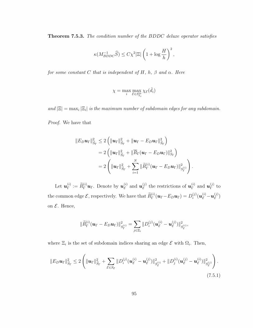
Theorem 7.5.3. The condition number of the BDDC deluxe operator satisfies
κ(M−1BDDCS) ≤ Cχ2|Ξ|
(1 + log
H
h
)2
,
for some constant C that is independent of H, h, β and α. Here
χ = maxi
maxE∈Sm
Ei
χE(di)
and |Ξ| = maxi |Ξi| is the maximum number of subdomain edges for any subdomain.
Proof. We have that
‖EDuΓ‖2SΓ≤ 2
(‖uΓ‖2
SΓ+ ‖uΓ − EDuΓ‖2
SΓ
)= 2
(‖uΓ‖2
SΓ+ ‖RΓ(uΓ − EDuΓ)‖2
SΓ
)= 2
(‖uΓ‖2
SΓ+
N∑i=1
‖R(i)Γ (uΓ − EDuΓ)‖2
S(i)Γ
).
Let u(i)Γ := R
(i)Γ uΓ. Denote by u
(i)E and u
(j)E the restrictions of u
(i)Γ and u
(j)Γ to
the common edge E , respectively. We have that R(i)Γ (uΓ−EDuΓ) = D
(j)i (u
(i)E −u
(j)E )
on E . Hence,
‖R(i)Γ (uΓ − EDuΓ)‖2
S(i)Γ
=∑j∈Ξi
‖D(j)i (u
(i)E − u
(j)E )‖2
S(i)E,
where Ξi is the set of subdomain indices sharing an edge E with Ωi. Then,
‖EDuΓ‖2SΓ≤ 2
(‖uΓ‖2
SΓ+∑E∈SE
‖D(j)i (u
(i)E − u
(j)E )‖2
S(i)E
+ ‖D(i)j (u
(j)E − u
(i)E )‖2
S(j)E
).
(7.5.1)
95

Denote by u(i)ΠE and u
(j)ΠE the restriction to E of the primal components corre-
sponding to u(i)Γ and u
(j)Γ . Since u
(i)ΠE = u
(j)ΠE , we have that
‖D(j)i (u
(i)E − u
(j)E )‖2
S(i)E≤ 2‖D(j)
i (u(i)E − u
(i)ΠE)‖
2
S(i)E
+ 2‖D(j)i (u
(j)E − u
(j)ΠE)‖
2
S(i)E,
and by (7.4.1),
‖D(j)i (u
(i)E − u
(j)E )‖2
S(i)E
+‖D(i)j (u
(j)E − u
(i)E )‖2
S(j)E≤
2‖u(i)E − u
(i)ΠE‖
2
S(i)E
+ 2‖u(j)E − u
(j)ΠE‖
2
S(j)E. (7.5.2)
Therefore, by combining (7.5.1), (7.5.2), and Lemma 7.4.9, we conclude that
‖EDuΓ‖2SΓ≤ C|Ξ|χ2
(1 + log
H
h
)2
‖uΓ‖2SΓ,
where |Ξ| = maxi |Ξi|. We conclude the proof of the theorem by using Lemmas
7.5.1 and 7.5.2.
7.6 Numerical results
Numerical examples are presented in this section to confirm the bound of The-
orem 7.5.3 for different types of subdomains, similar to what is done in Section
6.4. We consider a new Type 4 subdomain, with edges with both straight and
fractal segments. For these new subdomains, we divide the unit square into nine
squares and construct a fractal edge over each initial edge on the interface. We
note that the fractal segment lengths grow by a factor of 4/3 with each mesh re-
finement whereas the straight line segments remain constant. For each refinement
96

of Type 4 subdomains, every element edge on the fractal part of the boundary is
first divided into three shorter edges of 1/3 the length. The middle of these edges
is then replaced by two other edges with which it forms an equilateral triangle.
We call the number of partitions realized over the original straight edge the order
of the fractal. See Figure 7.1.
(a) Type 1 (b) Type 4
Figure 7.1: Two domain decompositions used in numerical examples.
To solve the resulting linear systems, we use a preconditioned conjugate gradi-
ent method to a relative residual tolerance of 10−8 with random right-hand sides.
The number of iterations and maximum eigenvalues estimates (in parenthesis) are
reported for each of the experiments. The condition number estimates are ob-
tained as mentioned in Section 1.2. We approximate the condition number by the
maximum eigenvalue, since the approximate value for the minimum eigenvalue is
always close to 1. We note that 1 is the minimum eigenvalue of our preconditioned
linear system; see e.g. [44, Lemma 6.4], [7, Lemma 3.4].
We recall that the numerical experiments for our algorithm show an improve-
ment in the iteration count and the condition number estimates, compared to an
iterative substructuring method presented in [19] and the two-level overlapping
97

Schwarz method considered in Chapter 6.
Example 7.6.1. We verify the scalability of our algorithm for Type 1 and 2 sub-
domains over the unit square. It is clear that the condition number is independent
of the number of subdomains, as shown in Table 7.1.
Table 7.1: Results for Type 1 and 2 subdomains, where the unit square is decom-posed into N subdomains, with H/h = 4, αi = 1 and βi = β. SE is the numberof subdomain edges, TE is the total number of degrees of freedom and ΓE thenumber of degrees of freedom on the interface. Number of iterations and conditionnumber estimates (in parenthesis) are reported for a relative residual tolerance of10−8.
Type N SE TE ΓE β = 10−3 β = 1 β = 103
1 64 112 3008 448 9(1.5) 8(1.5) 7(1.3)256 480 12160 1920 9(1.5) 9(1.5) 11(1.9)576 1104 27456 4416 9(1.5) 9(1.5) 10(1.8)
1024 1984 48896 7936 9(1.5) 9(1.5) 9(1.6)2 64 161 3008 735 10(2.0) 11(2.0) 9(1.5)
256 705 12160 3135 10(2.0) 10(2.0) 12(2.3)576 1633 27456 7199 10(2.0) 10(2.0) 13(3.1)
1024 2945 48896 12927 10(1.9) 10(1.9) 13(2.4)
Example 7.6.2. This example is used to confirm the logarithmic factor in the
bound of the condition number, for increasing values of H/h, with N = 16 subdo-
mains. For Type 4 subdomains, we approximate H/h by maxi√|dofi|; see Table
7.3. We have a growth in the condition number as expected; see Figures 7.2 and
7.3. We note that our algorithm does not require all subdomain edges to be of
comparable length, since Type 2 subdomains include edges both of order Hi and
hi.
98

10 20 30 401
1.5
2
2.5
3
3.5
4
4.5
H/h
Conditionnumber
Type 1 DD
β = 10−3
β = 103
15 20 25 30 35 40 451.2
1.3
1.4
1.5
1.6
1.7
1.8
1.9
2
2.1
2.2
H/h
Conditionnumber
Type 2 DD
β = 10−3
β = 103
Figure 7.2: Least-squares fit to a degree 2 polynomial in log(H/h) for data of Table7.2.
10 20 30 40 50 60 70 801
2
3
4
5
6
7
8
9
10
H/h
Conditionnumber
Type 3 DD
β = 10−3
β = 103
Figure 7.3: Least-squares fit to a degree 2 polynomial in log(H/h) for data of Table7.3.
99
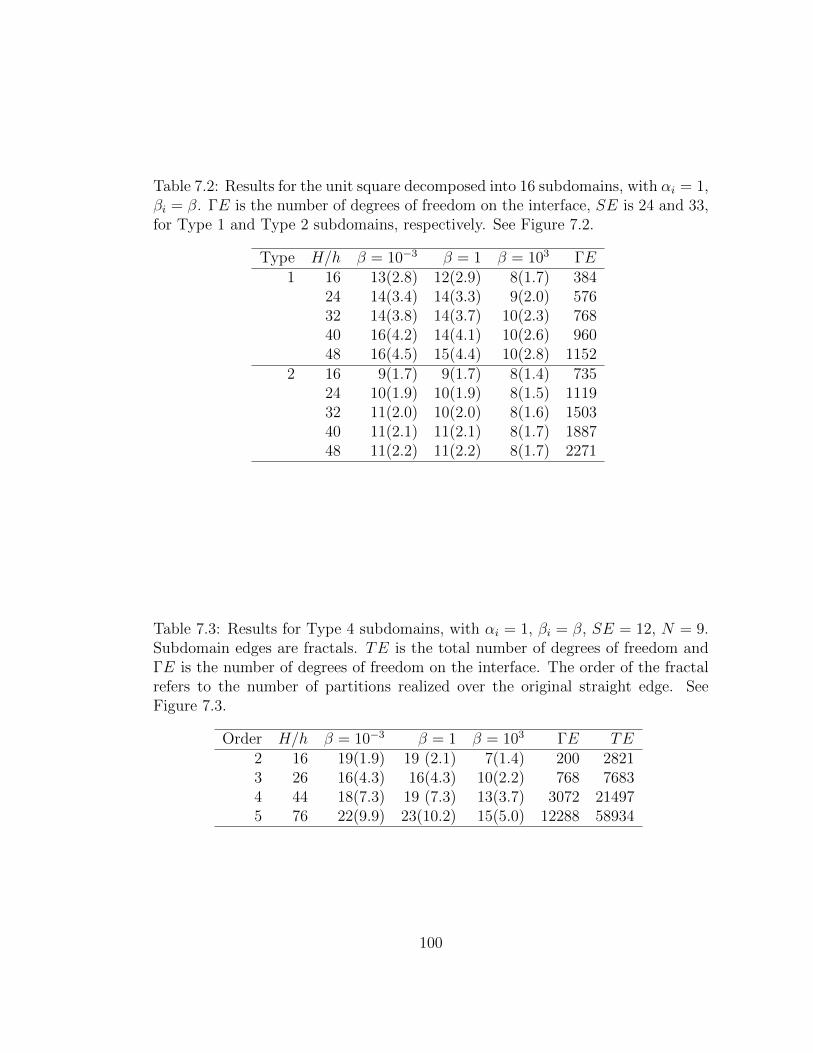
Table 7.2: Results for the unit square decomposed into 16 subdomains, with αi = 1,βi = β. ΓE is the number of degrees of freedom on the interface, SE is 24 and 33,for Type 1 and Type 2 subdomains, respectively. See Figure 7.2.
Type H/h β = 10−3 β = 1 β = 103 ΓE1 16 13(2.8) 12(2.9) 8(1.7) 384
24 14(3.4) 14(3.3) 9(2.0) 57632 14(3.8) 14(3.7) 10(2.3) 76840 16(4.2) 14(4.1) 10(2.6) 96048 16(4.5) 15(4.4) 10(2.8) 1152
2 16 9(1.7) 9(1.7) 8(1.4) 73524 10(1.9) 10(1.9) 8(1.5) 111932 11(2.0) 10(2.0) 8(1.6) 150340 11(2.1) 11(2.1) 8(1.7) 188748 11(2.2) 11(2.2) 8(1.7) 2271
Table 7.3: Results for Type 4 subdomains, with αi = 1, βi = β, SE = 12, N = 9.Subdomain edges are fractals. TE is the total number of degrees of freedom andΓE is the number of degrees of freedom on the interface. The order of the fractalrefers to the number of partitions realized over the original straight edge. SeeFigure 7.3.
Order H/h β = 10−3 β = 1 β = 103 ΓE TE2 16 19(1.9) 19 (2.1) 7(1.4) 200 28213 26 16(4.3) 16(4.3) 10(2.2) 768 76834 44 18(7.3) 19 (7.3) 13(3.7) 3072 214975 76 22(9.9) 23(10.2) 15(5.0) 12288 58934
100

Example 7.6.3. This example is used to demonstrate that the performance of
the algorithm need not diminish significantly when a mesh partitioner is used
to decompose the mesh. Example mesh decompositions for N = 16, N = 64 and
N = 144, shown in Figure 6.6, were obtained using the graph partitioning software
METIS, see [38]. Results are shown in Table 7.4.
Table 7.4: Comparison of results for Type 1 subdomains and subdomains generatedby METIS. Material properties are homogeneous with αi = 1, βi = β. For Type 1subdomains, H/h = 8. For subdomains generated by METIS, see Figure 6.6.
Type N β = 10−3 β = 1 β = 103 ΓE1 16 11(2.0) 11(2.0) 7(1.2) 192
64 11(2.1) 11(2.1) 10(1.8) 896144 11(2.2) 11(2.1) 12(2.4) 2112256 11(2.1) 11(2.1) 14(3.0) 3840400 11(2.2) 11(2.1) 14(2.8) 6080
METIS 16 18(8.9) 18(8.8) 9(1.6) 20464 27(10.7) 25(10.3) 12(2.3) 963
144 25(11.7) 25(11.7) 15(2.9) 2258256 25(15.0) 25(15.0) 19(4.9) 4061400 26(10.6) 26(10.6) 20(6.8) 6420
Example 7.6.4. This example is used to confirm that our estimate is indepen-
dent of the material property values in each subdomain. Insensitivity to jumps in
material properties is evident in Table 7.5. For the first set of experiments, the
subdomains along the diagonal have αi = α and βi = β, while the remaining sub-
domains have αi = 1 and βi = 1. We also include results with random coefficients,
where we generate random numbers ri1, ri2 ∈ [−3, 3] with a uniform distribution,
and assign αi = 10ri1 , βi = 10ri2 for all the elements inside each subdomain Ωi.
101
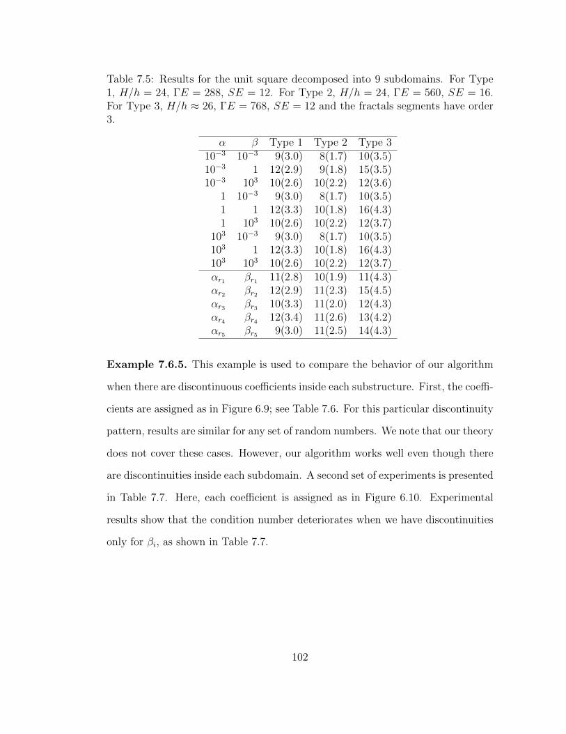
Table 7.5: Results for the unit square decomposed into 9 subdomains. For Type1, H/h = 24, ΓE = 288, SE = 12. For Type 2, H/h = 24, ΓE = 560, SE = 16.For Type 3, H/h ≈ 26, ΓE = 768, SE = 12 and the fractals segments have order3.
α β Type 1 Type 2 Type 310−3 10−3 9(3.0) 8(1.7) 10(3.5)10−3 1 12(2.9) 9(1.8) 15(3.5)10−3 103 10(2.6) 10(2.2) 12(3.6)
1 10−3 9(3.0) 8(1.7) 10(3.5)1 1 12(3.3) 10(1.8) 16(4.3)1 103 10(2.6) 10(2.2) 12(3.7)
103 10−3 9(3.0) 8(1.7) 10(3.5)103 1 12(3.3) 10(1.8) 16(4.3)103 103 10(2.6) 10(2.2) 12(3.7)αr1 βr1 11(2.8) 10(1.9) 11(4.3)αr2 βr2 12(2.9) 11(2.3) 15(4.5)αr3 βr3 10(3.3) 11(2.0) 12(4.3)αr4 βr4 12(3.4) 11(2.6) 13(4.2)αr5 βr5 9(3.0) 11(2.5) 14(4.3)
Example 7.6.5. This example is used to compare the behavior of our algorithm
when there are discontinuous coefficients inside each substructure. First, the coeffi-
cients are assigned as in Figure 6.9; see Table 7.6. For this particular discontinuity
pattern, results are similar for any set of random numbers. We note that our theory
does not cover these cases. However, our algorithm works well even though there
are discontinuities inside each subdomain. A second set of experiments is presented
in Table 7.7. Here, each coefficient is assigned as in Figure 6.10. Experimental
results show that the condition number deteriorates when we have discontinuities
only for βi, as shown in Table 7.7.
102

Table 7.6: Results for the unit square decomposed into 9 subdomains, with αi andβi discontinuous inside each subdomain, as shown in Figure 6.9.
Type H/h α = 1, βi disc. β = 1, αi disc. αi, βi disc.1 16 10(2.4) 12(2.8) 11(2.5)
24 11(2.9) 13(3.4) 11(2.9)36 11(3.4) 13(4.0) 13(3.4)
2 16 9(2.5) 10(1.9) 9(2.7)24 10(2.7) 10(2.0) 10(2.9)36 11(3.1) 11(2.1) 10(3.1)
4 16 13(4.5) 15(3.2) 15(5.1)26 14(5.7) 15(4.1) 14(5.6)44 16(7.1) 16(6.1) 16(8.1)
Table 7.7: Results for the unit square decomposed into 16 Type 1 subdomains,with H/h = 16, αi and βi discontinuous inside each Ωi and on its interface Γi, asshown in Figure 6.10.
Test α = 1, βi disc. β = 1, αi disc. αi, βi disc.1 35(86) 13(2.8) 35(106)2 52(613) 13(2.9) 37(482)3 47(332) 13(2.8) 35(69)4 39(119) 13(3.5) 36(64)5 55(626) 13(2.9) 54(606)
103

Chapter 8
An overlapping Schwarz
algorithm for Nedelec vector
fields in 3D
8.1 Introduction
In this chapter, we present a new coarse space for our problem in three dimen-
sions and some numerical results. We recall that previous studies for overlapping
Schwarz methods in 3D are very restrictive about the geometry of the subdomains.
To the best of our knowledge, the subdomains are usually tetrahedra or cubes, and
the coarse space is the usual Nedelec space defined on the coarse grid; see, e.g.,
[62, 33, 35]. Results for more general subdomains were obtained in [21], where a
BDDC method with deluxe scaling is analyzed.
In the next section, we introduce a new coarse space, valid for general sub-
domains. The two-level overlapping Schwarz algorithm with this new subspace
104
appears to be scalable, and independent of variations in H/h and of jumps in the
coefficients across the interface, and the condition number grows quadratically as
a function of H/δ, similar to the bound obtained in [62, 33].
We notice that we have tried several different approaches before, in order to
obtain an scalable algorithm for irregular subdomains. The coarse space described
in the following section is the only one that we have found to meet this requirement.
We present some numerical results without a theoretical analysis. We note that
we have some bounds for different functions that are part of a possible stable
decomposition, and we hope to complete the analysis in the near future.
8.2 A coarse space
We start by defining our coarse space V0. For each subdomain edge E , we define
a function cE as follows. First, we define λe(cE) = dE · te for e ⊂ E and λe(cE) = 0
for any other edge e on the wire-basket. Then, we extend these values over the
faces that have E on its boundary. For this purpose, let F ij be a face that has E
on its boundary, and consider the local matrices A(i) and A(j), where we partition
the degrees of freedom as
A(k) =
A
(k)C,C A
(k)C,F A
(k)C,∂F
A(k)F ,C A
(k)F ,F A
(k)F ,∂F
A(k)∂F ,C A
(k)∂F ,F A
(k)∂F ,∂F
,
105

for k ∈ i, j. Here, C represents the degrees of freedom in the complement of the
closure of the face. We then define
S(k)F ,F := A
(k)F ,F − A
(k)F ,CA
(k)C,C−1A
(k)C,F ,
and
S(k)F ,∂F := A
(k)F ,∂F − A
(k)F ,CA
(k)C,C−1A
(k)C,∂F .
These two matrices are blocks of the Schur complement of A(k) after that all the
degrees of freedom in the complement of the closure of the face are eliminated. We
then define the degrees of freedom for the face as
uF := −(S
(i)F ,F + S
(j)F ,F
)−1 (S
(i)F ,∂F + S
(j)F ,∂F
)u∂F .
We note that uF can be computed by solving a problem in Ωi ∪ Ωj. Finally,
we extend the values on the boundary of the subdomains harmonically into the
interiors of the subdomains, given the values over each local interface Γi.
8.3 Numerical Results
We present some numerical results for our two-level overlapping additive algo-
rithm. We consider a Type 1 decomposition, where the subdomains are cubes, and
a METIS decomposition (see Figure 8.1).
We solve the resulting linear systems using a preconditioned conjugate gradient
method and random right-hand sides, to a relative residual tolerance of 10−6. The
number of iterations and condition number estimates (in parenthesis) are reported
for each of the experiments. These estimates are obtained as mentioned in Section
106

1.2.
(a) Decomposition (b) Subdomain
Figure 8.1: Domain decomposition obtained by METIS for the unit cube, N = 27.
Example 8.3.1. We verify the scalability of our algorithm for Type 1 and METIS
subdomains over the unit cube. It is clear that the condition number is independent
of the number of subdomains, as shown in Table 8.1.
Table 8.1: Results for the unit cube decomposed into N subdomains, with αi = 1,βi = β, H/h = 8, H/δ = 4.
Type N β = 10−3 β = 1 β = 103 dof faces edges1 33 23(10.3) 24(10.5) 18(9.4) 102024 54 36
43 24(10.5) 25(10.9) 19(9.2) 238688 144 10853 24(10.6) 25(10.9) 21(9.2) 462520 300 24063 24(10.3) 25(10.8) 21(9.1) 795024 540 450
METIS 33 26(10.5) 26(10.8) 18(7.3) 102024 101 12643 28(12.2) 28(12.3) 19(7.5) 238688 287 38953 29(12.3) 30(14.5) 22(8.4) 462520 657 95163 29(12.4) 30(14.7) 22(8.5) 795024 1210 1804
Example 8.3.2. This example is used to study the behavior of our algorithm for
increasing values of H/h; see results in Table 8.2. We note that the condition
number is not sensitive to the mesh parameter H/h.
107

Table 8.2: Results for the unit cube decomposed into 64 Type 1 and METISsubdomains, with αi = 1, βi = β, H/δ = 4.
Type H/h β = 10−3 β = 1 β = 103 |dof | faces edges1 4 22(10.2) 24(11.4) 18(9.4) 31024 144 108
8 24(10.5) 25(10.9) 19(9.2) 238688 144 10812 25(10.7) 26(11.0) 20(9.3) 795024 144 108
METIS 4 29(13.5) 30(16.2) 20(8.5) 31024 291 3878 28(12.2) 28(12.3) 19(7.5) 238688 287 389
12 29(13.1) 29(12.9) 20(8.7) 795024 300 418
Example 8.3.3. This example is used to study the behavior of our algorithm for
increasing values of H/δ; see results in Table 8.3. Numerical results suggest a
quadratic growth of the condition number as a function of H/δ.
Table 8.3: Results for the unit cube decomposed into 27 Type 1 and METISsubdomains, with αi = 1, βi = β, H/h = 12.
Type H/δ β = 10−3 β = 1 β = 103
1 3 23(9.8) 24(9.7) 18(8.5)4 24(10.4) 25(10.8) 19(9.9)6 26(12.9) 27(12.9) 19(8.6)
12 31(24.9) 32(26.0) 21(10.4)METIS 3 26(9.9) 26(9.9) 20(7.9)
4 27(11.0) 27(10.9) 19(7.6)6 29(13.1) 30(13.8) 19(7.3)
12 36(20.3) 38(24.4) 20(8.0)
Example 8.3.4. This example is used to study the behavior of our algorithm for
discontinuous coefficients. Results are shown in Table 8.4. We include results with
random coefficients, where we generate random numbers ri1, ri2 ∈ [−3, 3] with a
uniform distribution, and assign αi = 10ri1 , βi = 10ri2 for all the elements inside
each subdomain Ωi.
108

Table 8.4: Results for the unit cube decomposed into 64 subdomains, with H/h =8, H/δ = 4.
α β Type 1 METIS10−3 10−3 22(8.6) 25(9.7)10−3 1 22(8.6) 25(9.6)10−3 103 19(8.3) 20(7.1)
1 10−3 23(10.4) 26(10.4)1 1 24(10.5) 26(10.8)1 103 21(9.4) 22(8.6)
103 10−3 23(9.0) 26(10.3)103 1 25(10.8) 27(10.2)103 103 23(8.5) 24(8.7)αr1 βr1 30(12.3) 30(12.2)αr2 βr2 26(10.9) 29(11.2)αr3 βr3 27(10.5) 28(11.1)αr4 βr4 30(12.0) 28(11.2)αr5 βr5 29(11.8) 29(10.2)
109

Bibliography
[1] D. N. Arnold, R. S. Falk, and R. Winther, Multigrid in H(div) and H(curl),
Numer. Math. 85 (2000), no. 2, 197–217.
[2] R. Beck, R. Hiptmair, R. H. W. Hoppe, and B. Wohlmuth, Residual based
a posteriori error estimators for eddy current computation, ESAIM: Math.
Model. Numer. Anal. 34 (2000), 159–182.
[3] B. Bojarski, Remarks on Sobolev imbedding inequalities, Lecture Notes in
Math. 1351 (1989), 52–68.
[4] A. Bossavit, Discretization of electromagnetic problems: The generalized finite
differences approach, Handb. Numer. Anal. 13 (2005), 105–197.
[5] D. Braess, Finite elements: Theory, fast solvers, and applications in solid
mechanics, Cambridge University Press, 2001.
[6] S. C. Brenner and R. Scott, The mathematical theory of finite element meth-
ods, Texts in Applied Mathematics, Springer, 2008.
[7] S. C. Brenner and L.-Y. Sung, BDDC and FETI-DP without matrices or
vectors, Comput. Methods Appl. Mech. Engrg. 196 (2007), 1429 – 1435.
110
[8] S. M. Buckley and P. Koskela, Sobolev-Poincare implies John, Math. Res.
Lett. 2 (1995), 577–593.
[9] J. G. Calvo, A two-level overlapping Schwarz method for H(curl) in two dimen-
sions for irregular subdomains, Tech. Report TR2014-968, Courant Institute,
NYU, 2014. Submitted to ETNA.
[10] , A BDDC algorithm with deluxe scaling for H(curl) in two dimen-
sions with irregular subdomains, Tech. Report TR2014-964, Courant Institute,
NYU, 2014. To appear in Math. Comp.
[11] L. Beirao da Veiga, L. F. Pavarivo, S. Scacchi, O.B. Widlund, and S. Zampini,
Isogeometric BDDC preconditioners with deluxe scaling, SIAM J. Sci. Comput.
36 (2014), A1118–A1139.
[12] R. Dautray and J.-L. Lions, Mathematical analysis and numerical methods for
science and technology. Vol. 2, Springer-Verlag, Berlin, 1988.
[13] , Mathematical analysis and numerical methods for science and tech-
nology. Vol. 1, Springer-Verlag, Berlin, 1990.
[14] T. A. Davis, Direct Methods for Sparse Linear Systems (Fundamentals of
Algorithms 2), Society for Industrial and Applied Mathematics, Philadelphia,
PA, USA, 2006.
[15] C. R. Dohrmann, A preconditioner for substructuring based on constrained
energy minimization, SIAM J. Sci. Comput. 25 (2003), 246–258.
111
[16] C. R. Dohrmann, A. Klawonn, and O. B. Widlund, Domain decomposition
for less regular subdomains: Overlapping Schwarz in two dimensions, SIAM
J. Numer. Anal. 46 (2008), 2153–2168.
[17] C. R. Dohrmann and O. B. Widlund, An overlapping Schwarz algorithm for
almost incompressible elasticity, SIAM J. Numer. Anal. 47 (2009), 2897–2923.
[18] , An alternative coarse space for irregular subdomains and an over-
lapping Schwarz algorithm for scalar elliptic problems in the plane, SIAM J.
Numer. Anal. 50 (2012), 2522–2537.
[19] , An iterative substructuring algorithm for two-dimensional problems
in H(curl), SIAM J. Numer. Anal. 50 (2012), 1004–1028.
[20] , Some Recent Tools and a BDDC Algorithm for 3D Problems in
H(curl), Domain Decomposition Methods in Science and Engineering XX
(R. Bank, M. Holst, O. B. Widlund, and J. Xu, eds.), Lecture Notes in Com-
putational Science and Engineering, vol. 91, Springer Berlin Heidelberg, 2013,
pp. 15–25.
[21] , A BDDC algorithm with deluxe scaling for three-dimensional H(curl)
problems, Comm. Pure Appl. Math (electronically published on April 28,
2015), doi: 10.1002/cpa.21574 (to appear in print).
[22] M. Dryja and O. B. Widlund, Schwarz methods of Neumann-Neumann type for
three-dimensional elliptic finite element problems, Comm. Pure Appl. Math.
48 (1995), no. 2, 121–155.
112

[23] C. Farhat, M. Lesoinne, P. LeTallec, K. Pierson, and D. Rixen, FETI-DP:
a dual-primal unified FETI method. I. A faster alternative to the two-level
FETI method, Int. J. Numer. Meth. Engng. 50 (2001), no. 7, 1523–1544.
[24] C. Farhat and F.-X. Roux, A method of finite element tearing and intercon-
necting and its parallel solution algorithm, Int. J. Numer. Meth. Engng. 32
(1991), no. 6, 1205–1227.
[25] H. Federer and W. H. Fleming, Normal and integral currents, Ann. of Math.
72 (1960), 458–520.
[26] A. George, Nested dissection of a regular finite element mesh, SIAM J. Numer.
Anal. 10 (1973), 345–363.
[27] J. R. Gilbert, Some nested dissection order is nearly optimal, Inform. Process.
Lett. 26 (1988), no. 6, 325–328.
[28] J. R. Gilbert and R. E. Tarjan, The analysis of a nested dissection algorithm,
Numer. Math. 50 (1987), no. 4, 377–404.
[29] V. Girault, Incompressible finite element methods for Navier-Stokes equations
with nonstandard boundary conditions in R3, Math. Comp. 51 (1988), no. 183,
55–74.
[30] V. Girault and P.-A. Raviart, Finite element methods for Navier-Stokes equa-
tions, Springer Series in Computational Mathematics, vol. 5, Springer-Verlag,
Berlin, 1986, Theory and algorithms.
[31] M. R. Hestenes and E. Stiefel, Methods of conjugate gradients for solving linear
systems, J. Research Nat. Bur. Standards 49 (1952), 409–436.
113
[32] R. Hiptmair, Multigrid method for Maxwell’s equations, SIAM J. Numer. Anal.
36 (1999), no. 1, 204–225.
[33] R. Hiptmair and A. Toselli, Overlapping and multilevel Schwarz methods for
vector valued elliptic problems in three dimensions, Parallel solution of Partial
Differential Equations (P. Bjørstad and M. Luskin, eds.), vol. 120 of IMA Vol.
Math. Appl., Springer, 2000, pp. 181–208.
[34] R. Hiptmair and J. Xu, Nodal auxiliary space preconditioning in H(curl) and
H(div) spaces, SIAM J. Numer. Anal. 45 (2007), 2483–2509.
[35] Q. Hu and J. Zou, A nonoverlapping domain decomposition method for
Maxwell’s equations in three dimensions., SIAM J. Numerical Analysis 41
(2003), no. 5, 1682–1708.
[36] F. John, Rotation and strain, Comm. Pure Appl. Math. 14 (1961), 391–413.
[37] P. W. Jones, Quasiconformal mappings and extendability of functions in
Sobolev spaces, Acta Math. 147 (1981), 71–88.
[38] G. Karypis and V. Kumar, A fast and high quality multilevel scheme for
partitioning irregular graphs, SIAM J. Sci. Comput. 20 (1998), 359–392.
[39] A. Klawonn, O. Rheinbach, and O. B. Widlund, An analysis of a FETI-DP
algorithm on irregular subdomains in the plane, SIAM J. Numer. Anal. 46
(2008), 2484–2504.
[40] T. V. Kolev and P. S. Vassilevski, Parallel auxiliary space AMG for H(curl)
problems, J. Comput. Math. 27 (2009), no. 5, 604–623.
114
[41] I. V. Lashuk and P. S. Vassilevski, The construction of the coarse de Rham
complexes with improved approximation properties, Comput. Methods Appl.
Math. 14 (2014), no. 2, 257–303.
[42] J. H. Lee, A Balancing Domain Decomposition by Constraints deluxe method
for numerically thin Reissner-Mindlin plates approximated with Falk-Tu finite
elements, SIAM J. Numer. Anal. 53 (2015), no. 1, 63–81.
[43] R. Leis, Initial-boundary value problems in mathematical physics, B. G. Teub-
ner, Stuttgart; John Wiley & Sons, Ltd., Chichester, 1986.
[44] J. Li and O. B. Widlund, BDDC Algorithms for incompressible Stokes equa-
tions, SIAM J. Numer. Anal. 44 (2006), 2432–2455.
[45] , FETI-DP, BDDC, and block Cholesky methods, Int. J. Numer. Meth.
Engng. 66 (2006), 250–271.
[46] R. J. Lipton, D. J. Rose, and R. E. Tarjan, Generalized nested dissection,
SIAM J. Numer. Anal. 16 (1979), no. 2, 346–358.
[47] J. Mandel and C. R. Dohrmann, Convergence of a Balancing Domain Decom-
position by Constraints and energy minimization, Numer. Lin. Alg. Appl. 10
(2003), 639–659.
[48] J. Mandel, C. R. Dohrmann, and R. Tezaur, An algebraic theory for pri-
mal and dual substructuring methods by constraints, Appl. Numer. Math. 54
(2005), 167–193.
[49] O. Martio and J. Sarvas, Injectivity theorems in plane and space, Ann. Acad.
Sci. Fenn. Ser. A I Math. 4 (1979), no. 2, 383–401.
115

[50] V. G Maz’ja, Classes of domains and imbedding theorems for functions spaces,
Soviet Math. Dokl. 1 (1960), 882–885.
[51] C. Muller, Foundations of the mathematical theory of electromagnetic waves,
Revised and enlarged translation from the German. Die Grundlehren der
mathematischen Wissenschaften, Band 155, Springer-Verlag, New York-
Heidelberg, 1969.
[52] J.-C. Nedelec, Mixed finite elements in R3, Numer. Math. 35 (1980), 315–341.
[53] D.-S. Oh, An overlapping Schwarz algorithm for Raviart-Thomas vector fields
with discontinuous coefficients, SIAM J. Numer. Anal. 51 (2013), 297–321.
[54] D.-S. Oh, O. B. Widlund, and C. R. Dohrmann, A BDDC algorithm for
Raviart-Thomas vector fields, Tech. Report TR2013-951, Courant Institute,
NYU, 2013.
[55] D. O’Leary and O. B. Widlund, Capacitance matrix methods for the Helmholtz
equation on general three-dimensional regions, Math. Comp. 33 (1979), 849–
879.
[56] A. Quarteroni and A. Valli, Domain decomposition methods for partial differ-
ential equations, Numerical mathematics and scientific computation, Claren-
don Press, 1999.
[57] , Numerical approximation of partial differential equations, Springer
Ser. Comput. Math., vol. 23, Springer, 2008.
[58] Y. Saad, Iterative methods for sparse linear systems, 2nd ed., SIAM, 2003.
116

[59] Y. Saad and M. H. Schultz, GMRES: a Generalized Minimal Residual Algo-
rithm for solving nonsymmetric linear systems, SIAM J. Sci. and Stat. Com-
put. 7(3) (1986), 856–869.
[60] H. A. Schwarz, Uber einen Grenzubergang durch alternierendes Verfahren,
Vierteljahrsschrift der Naturforschenden Gesellschaft, in Zurich, 1870,
pp. 272–286.
[61] B. F. Smith, P. E. Bjørstad, and W. D. Gropp, Domain decomposition: Par-
allel multilevel methods for elliptic partial differential equations, Cambridge
University Press, New York, NY, USA, 1996.
[62] A. Toselli, Overlapping Schwarz methods for Maxwell’s equations in three di-
mensions, Numer. Math. 86 (2000), 733–752.
[63] , Dual-primal FETI algorithms for edge finite-element approximations
in 3D, IMA J. Numer. Anal. 26 (2006), 96–130.
[64] A. Toselli and A. Klawonn, A FETI domain decomposicion method for edge
element approximations in two dimensions with discontinuous coefficients,
SIAM J. Numer. Anal. 39 (2002), 932–956.
[65] A. Toselli and X. Vasseur, Robust and efficient FETI domain decomposition
algorithms for edge element approximations, COMPEL 24 (2005), 396–407.
[66] A. Toselli and O. B. Widlund, Domain decomposition methods-algorithms and
theory, Springer Ser. Comput. Math., vol. 34, Springer, 2005.
117

[67] A. Toselli, O. B. Widlund, and B. Wohlmuth, An iterative substructuring
method for Maxwell’s equations in two dimensions, Math. Comp. 70 (2001),
935–949.
[68] L. N. Trefethen and D. Bau, Numerical linear algebra, SIAM, 1997.
[69] O. B. Widlund, Accommodating irregular subdomains in domain decompo-
sition theory, Domain Decomposition Methods in Science and Engineering
XVIII (M. Bercovier, M. J. Gander, R. Kornhuber, and O. B. Widlund, eds.),
Lecture Notes in Computational Science and Engineering, vol. 70, Springer-
Verlag, 2009, pp. 87–98.
[70] B. Wohlmuth, A. Toselli, and O. B. Widlund, An iterative substructuring
method for Raviart–Thomas vector fields in three dimensions, SIAM J. Numer.
Anal. 37 (2000), 1657–1676.
[71] J. Xu and Y. Zhu, Robust Preconditioner for H(curl) Interface Problems,
Domain Decomposition Methods in Science and Engineering XIX (Yunqing
Huang, Ralf Kornhuber, Olof Widlund, and Jinchao Xu, eds.), Lecture Notes
in Computational Science and Engineering, vol. 78, Springer Berlin Heidel-
berg, 2011, pp. 173–180.
118
Recommended