
Do institutional blockholders influence corporate investment? Evidence from emerging markets
Autores:
Roberto Álvarez
Mauricio Jara
Carlos Pombo
Santiago, Septiembre de 2018
SDT 469
1
Do institutional blockholders influence corporate investment?
Evidence from emerging markets
Roberto Alvareza, Mauricio Jaraa Carlos Pombob*
a School of Economics and Business, Universidad de Chile, Chile b School of Management- Finance Department, Universidad de los Andes, Colombia
Revised Version-R2 – August 15-2018
Abstract
This paper examines the relation between firm investment ratios and institutional blockholders for
a sample of 6,300 publicly traded firms in 16 large emerging markets for the 2004–2016 period.
Results show that independent, long-term, and local institutional investors boost investment ratios,
which is consistent with the monitoring role and blockholder voice intervention hypotheses. The
presence of institutional blockholders, regardless of their monitoring involvement, reduces firm
cash flow sensitivity ratios and thus reduces firms’ financial constraints. Minority institutional
investors complement the positive effect of blockholders investors. However, the effect on
financial constraints decreases as the quality of the country's institutions increases.
Keywords: Institutional Investors, Corporate Investment, Financial Constraints, Corporate
Governance, Emerging Markets
JEL codes: C20, G00, G20, G30
Email addresses: [email protected] (R. Álvarez), [email protected] (M. Jara-Bertin), and
[email protected] (C. Pombo)
* Corresponding author Carlos Pombo.
Address: Calle 21 # 1-20., Off. 917, Bogotá, Colombia
Phone: +57(1)-3394949 x. 3976
2
1. Introduction
One stylized fact within financial markets development during the last five decades has been the
increasing trend of institutional investor equity ownership across countries. The highest fraction
has been led within the United States, United Kingdom and Canada. For instance, institutional
ownership represented a 20% fraction within listed companies in United States in 1970. Forty years
later this number has risen to 65% (Borochin and Yang, 2017). The fraction of institutional
holdings within listed firms by 2007 was around 59% in Canada, 38% in the UK, 37% in Spain
and Sweden, 36% in Finland, and 31% in Norway and France (Aggarwal et al, 2011).
The presence and level of equity holdings by institutional investors within emerging markets has
risen, showing today similar levels to those observed in developed economies such as Australia or
New Zealand. In this study, we report for instance that institutional investor ownership represents
on average 21% in South Africa, 19% in Brazil and Poland, 12% in Chile, and 10% in Mexico for
the 2004-2016 period1.
This increase in institutional holdings coincides with the sophistication of financial markets, the
raising importance of corporate governance standards after structural financial reforms for equity
issuers around the world and the development of the private pension fund industry in several
emerging markets. For example, the OECD (2011) reported that the private pension fund industry
in Latin America that begun within economic openness programs in the 1990s, grew at an annual
rate of 16% between 1999 and 2006 to reach a net asset value of US$390 billion. Thus, these funds
constitute today dominant local investors in those equity markets.
The literature on institutional investors is extended and covers many aspects regarding their
ability to be an informed investor, their monitoring role and activism to influence corporate policies
1 See table Appendix B.
3
such as executive compensation, firms’ board of director structures, shareholder’s voting schemes,
anti-takeovers amendments among other shareholder proposals. This ability of institutional
investors in gather information contribute to the development of capital markets by stimulating
efficient transactions, good risk evaluation, and a sound corporate governance system. They can
also exert a direct influence through their ownership (shares) by direct monitoring to discipline
firm management and exert an indirect influence through their ability to sell their shares (Gillan
and Starks, 2003, 2007).
Empirical research during the last 10 years highlights several advantages derived from the
presence of institutional investors in firms’ ownership structure on firm asset value, firm
performance, cost of equity, demand for information disclosure and firm-specific corporate
governance standards. The main findings state that increasing institutional ownership explain
higher firms’ value premiums (Ferreira and Matos, 2008), effective reduction on corporate bond
yield spreads (Elyasiani et al. (2010), and changes in firm-level governance over time due to
previous changes foreign institutional ownership, investors who promote higher governance
standards within low investor protection countries (Agrawal et al, 2011). Also, there is evidence
concerning positive shocks of institutional ownership on increasing firms’ quantity, form, and
quality of corporate disclosure. (Bird and Karolyi, 2016).
Studies on institutional investor heterogeneity is other topic that has brought attention within
recent years. This research stresses the monitoring role of institutional investor in reducing
informational asymmetries and shareholder agency costs. Investor heterogeneity implies that not
institutional investors are alike. Their effect on ex-post firm performance might differ because of
portfolio turnover, holding concentration, and the degree of incentives to exert intensive monitoring
to firms’ management by institutional investors. Monitoring incentives becomes a function of the
4
potential business relations that institutional investors might involve within firms they invest in
(Ferreira and Matos, 2008).2.
Previous research on multiple blockholder ownership in general and institutional ownership in
particular, have not explored in detail the direct and interacted effects of institutional holdings on
corporate investment in a broader sense that includes capital expenditures, acquisitions and
spending in research and development with focus on emerging markets. First, the effect on firm
value due to presence of multiple blockholders has been empirically documented in studies across
markets and countries (Maury and Pajuste (Finland), 2006; Laeven and Levine (Europe), 2008;
Attig et al. (East Asia), 2009). These studies consistently show that a less dispersed distribution of
votes among large blockholders had a positive effect on firm value, that value is enhanced when
there are multiple blockholders. In the same vein results on the marginal effects of blockholder
identity and firm value confirm that the kind of second blockholder is vitally important when it
comes to contesting the agency costs of controlling owners for different study samples (Jara-Bertin
et al., (Continental Europe) 2008; Sacristan et. al. (Spain) 2015; Pombo and Taborda (Latin
America) 2017).
Second, studies on relational investing analyse the role of institutional investors as blockholder
on corporate investment as consequence of a long-term partnership relation between outsider
investors (e.g. institutional) and companies. These studies in short find that institutional
blockholders are generally correlated with lower executive pay levels (Hartzell and Starks, 2003),
higher investment (Cronqvist and Fahlenbrach, 2009), and less opportunistic earnings management
2 This work and similar studies claim that independent institutional investors (investment funds and investment
advisors) actively monitor firms’ management, while grey investors are more prone to be more loyal to corporate
management and thus to hold shares without reacting to management actions that are not in line with the interests of
shareholders. These studies show a positive effect in changes of institutional holdings by independent investors on
firms’ Tobin’s Q, and the effect of grey investors is non-conclusive and statistically not significant. Other studies refer
to institutional investor heterogeneity as “active/passive” investors (Almazan, 2005); “pure resistant/sensitive”
investors (Brickley 1988); “dedicated/transient” investors (Borochin and Yang, 2017).
5
in firms because the institutional investors put pressure on the firms to adopt better accounting
policies (Chung et al., 2002). Other studies have found that institutional blockholders are associated
with higher profitability and superior M&A outcomes (Chen et al., (2007) and on the effects that
institutional investors have on firms’ R&D investment. Brav et al., (2016) find that hedge funds
activism leads to lower firm R&D spending but raises in both the number of future patents and
their quality, which lead them to conclude that hedge funds improve innovation efficiency.
Third, studies on firm financial constraints supported by the predictions of information
asymmetries in capital markets, hypothesize that agency costs faced by outside investors lead firm
management to choose suboptimal investment choices (i.e., overinvestment and underinvestment
rates) and become more dependent of lower cost internal funding. Benchmark cash flow sensitivity
studies have concentrated on the interactions with operating cash flow of inside ownership
(Hadlock, 1998) or family holdings (Pindado et al., 2011).
Forth, despite the above extended literature there are just two close studies with our work on
institutional blockholder ownership and corporate investment, but restricted to samples of US
firms. The first by Lev and Nissim (2003) studies how institutional ownership concentration
reduces informational asymmetries that mitigates firm hangout (underinvestment) problem. Their
main findings provide evidence that institutional blockholder ownership level impact positively
firm investment either if investors are classified by dedicated (long term) or transient (short term)
investor and reduces firm financial constraints for acquisitions and investments in R&D. The
second study by Richardson (2006) provide evidence that overinvestment is common across firms

6
with higher levels of cash flow and it is reduced by institutional blockholder ownership and by
shareholder activism.3
The present study empirically evaluates the impact of institutional investors on investment
decisions. If institutional investors are related to investment decision-making and improvements in
corporate governance, their presence may stimulate more investment. We consider the effect of
minority institutional holdings that behave more as a retail investor on investment and examine the
effect of institutional investors as blockholders on the sensitivity of investment demand on internal
resources (operating cash flow) as a proxy of firms’ financial constraints.
The article makes a twofold contribution to the empirical literature on institutional investors.
First, the paper fills a research gap by looking at whether the monitoring of institutional blockholder
ownership (presence) increases firm investment and how investor heterogeneity affects firm
investment ratios using reduced cash flow sensitivity as a proxy of firm financial constraints. We
further current understanding of investor heterogeneity by looking not only at the monitoring role
played by institutional investors (i.e., investor colours) but also at other features of blockholder
characteristics such as investors’ horizon and origin location. When analysing investment
regressions, we also consider minority institutional holds, which are present in 70% of this study
sample of firms. Thus study extends prior work addressing institutional investor heterogeneity and
firm financial constraints by focusing on the relations between institutional blockholder ownership
and firm investment ratios.
Second, corporate governance reviews have stressed that the role of institutional investors in
discipline management in emerging markets is understudy because there is no solid evidence on
3 Firm governance attributes in Richardson’s (2006) study are factor score indices. Shareholder activism index
comprises the number of activist shareholders (public pension funds), percentage held by activist shareholders and the
fraction of outstanding shares held by the average outside director.

7
their behavior (Claessens and Yurtoglu, 2013). This study focuses on emerging markets where
evidence is limited regarding the strategic role that institutional investors play on firms’ investment
dynamics. Our sample covers 16 major emerging markets representing the main markets from East
Asia, Latin America, East Europe and South Africa.4
Our results confirm that blockholder institutional investor ownership increases investment
spending, although the relation is not linear. The inflexion point of a positive effect is around 0.22
of institutional holdings of a firm’s outstanding shares. Thus, when institutional blockholders have
no control over the firm they put pressure on current investment in order to obtain short- and
medium-term returns (Gompers and Metrick, 2001). Once the threshold is surpassed, institutional
blockholders lack sufficient incentives to put pressure on current investment. In this scenario,
institutional investors exert control on over-investment, which is in line with the result reported by
Ferreira and Matos (2008) in the sense that firms with greater independent institutional ownership
decrease firms’ capital spending and control over investment behaviour.
Regression estimates show that 1 standard deviation change in institutional blockholder
ownership increases investment ratios by 240 base points for the total sample and by 220 base
points, excluding China. Investor heterogeneity regressions confirm that independent investors
drive the marginal effect. The marginal effect of grey investors is not statistically significant in
generalized method of moments (GMM) regressions. Independent investors have an effect in the
short run when they do not sell their equity shares within one year. The size effect of their short-
term holdings is, on average, 0.11. For long-term holdings, when investors remain for two or more
years, the size effect increases to 0.23. In contrast, the effect of grey investor portfolio duration is
4 South Africa as the only African country member of the BRICS association. The acronym BRIC was originally
coined in 2001 by Goldman Sachs asset management to group the largest and fastest growing emerging economies,
specifically, Brazil, Russia, India, and China. In 2010 South Africa joined the BRICS association.

8
not significant. Thus, their role in controlling suboptimal corporate investment spending remains
inconclusive. Investor origin estimates show that local institutional ownership is a significant
regressor in explaining firm investment ratios, while foreign ownership does not exert effective
monitoring on the firm. This result is partially explained by the low fraction of equity ownership
held in the hands of foreign institutional investors as blockholders relative to local institutional
blockholders.
Results also show that minority institutional ownership complements the blockholder investor
effect. The overall marginal effect is around 0.18, meaning that a 1 standard deviation change in
minority holdings increases investment ratios by an additional 86 base points.
Investment cash flow sensitivity results show that institutional investors reduce firms’ dependence
on internal resources (i.e., operating cash flow) for funding investment. These results are consistent
with the hypothesis that direct intervention by institutional blockholders reduces information
asymmetries and enhances corporate disclosure. The presence of institutional blockholders also
entails greater access to external borrowing.
The remainder of this paper is structured as follows. Section 2 presents the sample construction
and method and includes the description of the dependent and explanatory variables as well as a
discussion of the regression baseline estimating equation. Section 3 presents the econometric
results of the baseline investment equation. Section 4 provides a robustness analysis of the baseline
investment regressions through cross sectional tests by splitting the sample according to the
heterogeneity in firms’ financial constraints. Finally, section 5 offers our conclusions.
2. Data and method
2.1 Sample construction
9
The working dataset comprises firm-level information from Thomson Reuters Eikon. The raw data
sample includes 7,253 firms from 16 emerging economies with 63,303 firm-year observations of
annual financial and shareholder ownership information for the period 2004 to 2016. The sample
used in the estimations has the following characteristics. First, it focuses only on nonfinancial
firms. Therefore, we exclude all firms that belong to the Thomson Reuters Business Classification:
Banking and Investment Services, Uranium, Insurance and Real State companies. Second, we
exclude firms with less than three years’ coverage as well as firms with missing values for
ownership features, capital expenditures, sales, assets, debt, cash flow, and stock prices. Third,
following Hadlock and Pierce (2010), we exclude observations with investment to assets ratios of
above 2.0 and sales to assets ratios above 4.5 so as to remove potential outliers. Fourth, we drop
outliers in the top and bottom 1% of each variable. The final sample is thus an unbalanced panel
of 46,8585 observations from 6,422 listed nonfinancial firms from 16 emerging markets6.
Table 1 provides the descriptive statistics for investment, cash flow and institutional ownership,
as well as the main control variables included in the econometric analysis for the total sample and
selected subsamples. The first subsample excludes China since it represents 37% of the total
sample. The second subsample is the set of firms with institutional blockholder investors, and the
third subsample only includes firms with minority institutional blockholder investors. The table
provides several interesting insights. First, institutional investors are blockholders in 22% of the
5 The total dataset length with investment records is 46,858 firm-year observations. This number is greater than the
total sample for either total investment or adjusted investment regressions, which is around 35,600 firm year
observations. This difference is because investment ratios are normalised by the lag of total assets and a lag of the
dependent variable is introduced. Thus, there are two lags in all the regression estimates.
6 The total sample by country is: Brazil (n=1147), Chile (n=942), China (n=17,234), Colombia (n=86), Greece
(n=1,273), Hungary (n=133), Indonesia (n=2,078), Malaysia (n=5,164), Mexico (n=645), Peru (n=335), Poland
(n=2,084), Republic of Korea (n=10,227), Saudi Arabia (n=575), South Africa (n=1,549), Thailand (n=3,063), and the
United Arab Emirates (n=323)

10
total sample with average equity rights of 14%. In contrast, minority institutional investors are
present in 70% of the total sample, with average equity rights of 5.1%.
Second, firms with institutional blockholders have greater investment ratios (0.072) than the
total sample (0.069) or the subsample that excludes China (0.062). Regardless of whether or not
there are institutional blockholders, firms with minority investors display the highest investment
rates (0.075). Third, the sample with minority institutional ownership exhibits higher firm valuation
than the firms in the other subsamples. The mean of Tobin’s Q is 1.45 whereas for the total sample
it is 1.33. For the subsample that excludes China it is 1.08. This is to be expected because, where
they are minor institutional investors, institutional investors tend to invest more in high value firms.
Finally, firms with institutional blockholders are, on average, bigger, have higher cash flow ratios,
and are less indebted. Descriptive statistics across countries exhibit similar patterns7.
[TABLE 1 ABOUT HERE]
2.2 Methodology
The main focus of the empirical approach is to analyse the effect of institutional investor
blockholders on investment decisions by gauging the potential impact institutional investors have
on relaxing financial constraints. We estimate an extended version of Fazzari et al. (1988)
investment model to test the relevance of institutional investors on investment decisions. Empirical
literature on corporate investment has shown that cash flow is a good predictor of investment when
a wedge exists in the financing costs between internal and external sources of funds. This would
occur because financial markets tend to exhibit some frictions such as credit rationing and adverse
selection problems due to information asymmetries (Myers and Majluf, 1984). Hence, the higher
the funding costs wedge, the more financial constraints on the firms and the more investment
7 In particular, institutional investor presence is more relevant in Brazil, Poland and South Africa. These statistics are
reported in table appendix B.
11
decisions explained by internal cash flow. As such, greater dependence on internal funds can lead
firms to invest sub-optimally.8 However, Kaplan and Zingales (1997) cast doubts on the usefulness
of the investment cash flow model to capture financial constraints. This finding opened a keen, yet
thus far unresolved debate regarding the usefulness of certain metrics for capturing financial
constraints (Allayannis and Mozumdar, 2004).
Following Laeven (2003) and Aguiar (2005), the empirical baseline investment regression equation
is
𝐼𝑛𝑣𝑖,𝑡 𝑜𝑟 𝐼𝑛𝑣. 𝑎𝑑𝑗𝑖,𝑡 = 𝛽1 𝐼𝑛𝑣𝑖,𝑡−1 + 𝛽2 𝐼𝑂𝑤𝑛𝑖,𝑡 + 𝛽3 𝐼𝑂𝑤𝑛𝑖𝑡2 + 𝛽4 𝐼𝑂𝑤𝑛𝑖𝑡 × 𝐶𝐹𝑂𝑖𝑡 +
𝛽5 𝑀𝑖𝑛. 𝐼𝑂𝑤𝑛𝑖,𝑡 + 𝛽6 𝐶𝐹𝑂𝑖,𝑡 + 𝛿𝑘𝐗𝑖,𝑡−1 + 𝐼𝑗𝑡 + 𝑦𝑐𝑙𝑡 + 𝑢𝑖𝑡 , (1)
where subscript i stands for the firm, j for industry, l for country, and t for year. The dependent
variable 𝐼𝑛𝑣𝑖𝑡 is total firm investment and is computed as the sum of capital expenditures,
acquisitions and R&D expenses, minus sales of PPE of firm i in year t over total assets at the
beginning of the period (Richardson, 2006). Thus, total investment ratio is computed as follows:
𝐼𝑛𝑣𝑡 =(𝐶𝐴𝑃𝐸𝑋𝑡 + 𝐴𝐶𝑡 + 𝑅𝐷𝑡 − 𝑆𝑎𝑙𝑒𝑠𝑃𝑃𝐸𝑡
)
𝐴𝑠𝑠𝑒𝑡𝑠𝑡−1 (2)
We also include industry adjusted ratios (𝐼𝑛𝑣. 𝑎𝑑𝑗𝑖,𝑡), as the dependent variable, computed as the
total investment ratio scaled up industry-country median out of the total investment ratio in year t.
That is
𝐼𝑛𝑣. 𝐴𝑑𝑗𝑡 =𝐼𝑛𝑣𝑡
𝑀𝑒𝑑𝑖𝑎𝑛 𝐼𝑛𝑣𝑗𝑡 (3)
8 For instance, firm overinvestment is associated with excess cash flow or the underinvestment problem due to agency
costs of debt or debt overhang.
12
To control investment ratios by financial constraint, the empirical equation includes cash from
operating activities of firm i in year t over total assets at the beginning of the period - 𝐶𝐹𝑂𝑖𝑡-. As
regard institutional ownership variables, 𝐼𝑂𝑤𝑛𝑖𝑡 represents institutional investor ownership in the
hands of institutional blockholders (IOwn) (over 5%); 𝑀𝑖𝑛. 𝐼𝑂𝑤𝑛𝑖𝑡 represents total institutional
ownership in the hands of minority shareholders (below 5%). Vector X includes the set of lagged
control variables commonly used in previous studies such as firm Tobin’s Q (Tobin’s Q) as a proxy
of investment opportunities, firm size (Size), debt ratio (Debt), cash and short-term investments
scaled total assets (Cash), and sales ratio (Sales). Following prior empirical estimates, in order to
control for market liquidity, we include a dummy variable that takes the value 1 if a firm belongs
to the most traded local index in the year t (e.g., IPSA, BOVEPSA, KOSPI, among others), and
zero otherwise9.
The empirical investment equation includes a set of fixed effects at different aggregation levels
to control for unobservable time-invariant and time-variant fixed effects. In particular, an industry
fixed effect (𝐼𝑗) captures the impact of unobservable factors at the industry-level affecting
investment decisions. In addition, we include a set of country-year fixed effects (𝑦𝑙𝑡) to capture
country time-variant determinants of investment, such as GDP growth and inflation, among others.
One concern about institutional ownership stems from the endogeneity associated with investor
preferences that bias firm value or investment regression estimates. Empirical evidence shows that
institutional investors invest more in large firms, and in firms with a good corporate governance
reputation. Furthermore, they prefer firms that show higher market valuations, better operational
performance, and lower capital expenditure (Ferreira and Matos, 2008). However, to attenuate this
problem, in some estimations, we only focus on those institutional investors that can engage in
9 Appendix A provides the definitions of all the variables considered in the empirical analysis. The online
supplementary reports the partial correlations across the explanatory variables included in the regression estimates.

13
monitoring through significant ownership holdings. Specifically, we define institutional ownership
as the sum of all ownership held by any institutional investor blockholder (IOwn). When a stand-
alone institutional investor does not meet the 5% threshold, we compute the institutional investor
as zero. We also include, separately, the potential effect on investment of institutions defined as
having minority institutional ownership, computed as the sum of all ownership held by any
institutional investor categorized as a minority investor (a less than 5% stake). When a stand-alone
institutional investor exceeds the 5% threshold, we compute the institutional investor as zero.
There are three main arguments concerning the relation between institutional investor ownership
and firm investment. First, the monitoring approach suggests that when institutional investors
become blockholders, they have greater incentives to gather information, monitor controllers, and
demand both more and better investment to improve firm value (Cornett et al., 2007; Maug, 1998).
They can use the voice mechanism or the threat of exit to demand greater investment, consistent
with arguments related to investor demand for investment aimed at securing superior firm value
(Gompers and Metrick, 2001; Marie and Bastien, 2009).
Second, institutional investor ownership restricts overinvestment problems in firms that are
more likely to suffer from it, such as in cases of excess cash flow within large firms. This argument
predicts a negative relation between institutional investors’ holdings and industry-adjusted
investment (Ferreira and Matos, 2008).
Third, a negative relation between institutional ownership and investment is also predicted when
institutional blockholders can worsen corporate decisions because of their propensity to extract
private benefits (Edmans, 2014). This likelihood increases when institutions wield greater power
in the firm, which exacerbates the agency conflict between institutional investors and other large
shareholders, leading to non-maximizing corporate actions such as asset substitution and
underinvestment. Ruiz-Mallorquí and Santana-Martín (2011) show that when institutional
14
investors are banks, the effect on firm value is negative because dominant shareholders tend to
strength their business relationship in order to extract private benefits. However, they find that
when institutional investors are investment advisors, they tend to improve the firm’s value. This
positive effect on firm value may be related to incentives to avoid inefficiencies such as
overinvestment. However, both arguments—private benefit extracting or efficiency in avoiding
overinvestment—predict a negative relation between high institutional ownership and corporate
investment.
Thus, in order to analyse whether nonlinear effects are important in generating an inverted U-
shaped relation between the level of institutional equity holdings and firm investment ratio, we
introduce a quadratic term for the institutional investor variable. The coefficients 𝛽2 and 𝛽3 in Eq.
1 should be negative and positive, respectively.
The empirical model takes into account whether institutional investor heterogeneity matters vis-
à-vis explaining investment decisions. Thus, we distinguish institutional holdings between investor
colours (i.e., grey vs. independent investor) and origin (i.e., domestic vs. foreign investor), and
introduce the variables of institutional orientation type and their interactions with cash flow.
The monitoring argument highlights the beneficial influence of institutional investors on firm value
(Elyasiani et al., 2010; Hartzell et al., 2014). This beneficial effect depends exclusively on
institutional investor ability to attenuate asymmetrical information issues or to successfully
influence controllers or managers to make value-creating decisions (Almazán et al., 2005) or to
avoid overinvestment problems. Of course, as Ferreira and Matos (2008) show, independent
institutional investors may be more likely to spend greater resources on monitoring activities or to
have fewer potential business relationships with the corporation in which they invest. We define
independent investor ownership (IndIO) as the sum of blockholder ownership held by mutual fund
15
managers and investment advisor firms, and we expect that if independent investors engage (do
not engage) in monitoring activities, firms should display higher (lower) levels of investment.
On the other hand, grey investors are less likely to exert the voice mechanism because they
maintain business ties with company managers and may attempt to increase their control of the
firm. We define grey investor ownership (GreyIO) as the sum of blockholder equity holdings by
institutions classified as grey (i.e., bank trusts, insurance companies, pension funds, and
endowments). De-la-Hoz and Pombo (2016) report for Latin America a discount of 0.12 units on
firms’ Tobin’s Q when grey institutional investors are the largest blockholder. This finding
suggests that for firms whose largest shareholder is a grey investor, management may take on non-
value-maximizing investments, and thus the expected relation is positive or non-significant.
We also analyse whether institutional investors increase or decrease financial constraints. In that
sense, we expect the coefficient 𝛽5 for operating cash flow (CFO) to be positive in all the
specifications according to the literature. In the presence of financial constraints, an increase in
cash flow should increase investment. More importantly, institutional investors can shape financial
constraints by alleviating or increasing asymmetric information through incentives to monitor
controllers and managers. This effect is captured by introducing the interacting term of institutional
ownership and firm cash flow in the estimating equation.
Two arguments can moderate the relation between the type of institutional investor blockholders
and financial constraints. First, when institutional investors become blockholders, they will engage
in corporate governance activities to ensure value-maximizing decisions. If the monitoring
argument prevails, we expect institutional blockholders to reduce financial constraints and, hence,
the expected sign for the coefficient 𝛽4 when estimating Equation 1 to be negative. Second, as
previously mentioned, institutional investors can influence managers to make nonvalue-
maximizing decisions such as overinvesting or underinvesting so as to extract private benefits. This
16
influence may be critical when institutions control the firm. If the expropriation argument
dominates, institutional blockholders will increase financial constraints, and so the sign for
coefficient 𝛽4 will be positive.
Due to endogeneity problems in dynamic panel data, ordinary least squares estimators can
produce biased coefficients; for this reason, we use generalized method of moments (GMM). The
GMM system estimator deals with the endogeneity issues inherent in the relation between
investment and cash flow. In general, all right-hand variables are potentially endogenous (Pindado
et al. 2011). One important feature of the GMM method is that it controls for endogeneity of all
firm-level variables by introducing lagged right-hand side variables as instruments. Specifically,
we introduce all right-hand side variables lagged from t–2 to t–4 when estimating Equation 1. Thus,
the GMM system estimator offers some advantages over other dynamic panel models that are
regularly used in corporate finance research (Flannery and Hankins, 2013).
The consistency of the estimates depends on the absence of second-order serial autocorrelation
in the residuals and on the validity of the instruments. Accordingly, we report p-values of the first
and second order autocorrelation test. To test the validity of the instruments, we use the Hansen
test of over-identifying constraints, which tests for the absence of correlation between the
instruments and the error term and, therefore, checks the validity of the selected instruments.
3. Econometric results
3.1. Institutional blockholders and minority institutional investors
This section reports the findings on whether institutional investors influence investment decisions
and their effect on the cash flow sensitivity relation. Table 2 shows the baseline results for the
institutional investor ownership variable for the whole sample and for the subsample that excludes
17
China. Three main findings should be highlighted. First, institutional blockholder ownership is
statistically significant in its own term (IOwn) as well as in its squared term (IOwn2) across
specifications. The size of marginal effect is relevant in the presence of non-linear relation of
institutional blockholder ownership and controlling by firm operative cash flows. The marginal
effect ranges from 𝛽2 = 0.26 (Col.1) to 0.30 (Cols. 5)10. This later estimate says that 1 standard
deviation change in institutional blockholder ownership, firm investment ratios rise by 2.4%.11 If
we replace total investment with an industry-adjusted measure of total investment (columns 6 to 8
and 12 to 14 for the total sample and excluding China, respectively) the results are qualitatively
similar to previous findings. These regressions are controlled by minority institutional holdings
(Min-IOwn) for all cases.
The above findings indicate an inverse U-shaped relation between institutional blockholder
ownership and investment ratios and suggest that, at low levels of institutional blockholder
ownership, investors positively influence firm investment. These results confirm that institutions
have incentives to demand more and better investment when they act as blockholders. Institutional
investors’ “voice” and the threat of exit account for the monitoring incentives of institutions to
ensure value-maximizing decisions related to investment (Gompers and Metrick, 2001; Marie and
Bastien, 2009).
Second, using both dependent variables (Inv and Inv. Adj.) the nonlinear relation indicates the
existence of an average threshold point of institutional investors ownership of around 21.2% and
19.5% for the full sample (Col.2 and 8) and excluding China (Col.5 and 11), respectively. Above
10 The marginal effect of institutional blockholder ownership in Col. 5 is 𝜕𝐼𝑛𝑣 𝜕𝐼𝑂𝑤𝑛 = 𝛽2 − 2𝛽3 ∙ 𝐼𝑂𝑤𝑛⁄ .
Therefore: 𝜕𝐼𝑛𝑣 𝜕𝐼𝑂𝑤𝑛 = 0.355 − 2 × 0.798 × 0.032 = 0.304⁄ where 0.032 is the mean of IOwn for the full
dataset length reported in Table 1. 11 The change in the investment ratio due to 1 standard deviation in institutional ownership is 0.304 × 0.079 =0.024 = 2.4%. Excluding China, that effect is 2.2%
18
that point, institutional investors can take advantage of a dominant position to extract private
benefits (i.e., dividend clientele effect) and thus lower firm investment spending (Edmans, 2014).
An alternative explanation is an efficiency argument that is related to institutional investor
incentives to restrict overinvestment problems (Ferreira and Matos, 2008).12
Third, institutional ownership reduces financial constraints. The operating cash flow coefficient
𝛽6 (CFO) is positively associated with investment across regressions. Cash flow sensitivity is 0.065
for the total sample (Col. 3) and 0.068 excluding China (Col. 9), while the regression coefficient
𝛽4 for the interacting term 𝐶𝐹𝑂 × 𝐼𝑂𝑤𝑛 is negative and statistically significant for the total sample
and without China, respectively. The quantitative relevance of institutional blockholder ownership
is significant. Indeed, firm financial constraints drop by 60 base points for the total sample and 320
excluding China. Marginal effects are evaluated at sample means of institutional blockholder
ownership13
This finding corroborates the intuition that institutional blockholders actively participate in
corporate governance. Boone and White (2015) show that institutional investors enhance
monitoring capabilities by increasing transparency and improving managerial disclosure and
liquidity, resulting in lower information asymmetry. Bird and Karolyi (2016) find that positive
changes in institutional investors increase the volume and quality of firm disclosure. These results
are consistent with the view that investors have incentives to gather information, monitor, and
12 We cannot differentiate between the “efficient” and “private benefits” arguments to explain the negative relation at
high levels of institutional ownership. 13 Marginal effects are evaluated in this case at the variable’s sample mean based on the regression equation number
of observations. The marginal effect of operating cash flow (CFO) evaluated at sample mean of institutional
blockholder ownership (IOwn) in Col. 5 is 𝜕𝐼𝑛𝑣 𝜕𝐶𝐹𝑂 = 𝛽6 + 𝛽4 × 𝐼𝑂𝑤𝑛 = 0.059⁄ ; The marginal effect of CFO
without the interacting term CFO x IOwn in Col. 3 is 𝛽6 = 0.065. Therefore, the difference in investment cash flow
sensitivities between both regressions is 0.065 0.059 = 0.006 or 60 base points. Similarly, the marginal effect for the
subsample that excludes China in Col.11 is 𝜕𝑦 𝜕𝐶𝐹𝑂 = 0.036⁄ , and the marginal effect of CFO in Col. 9 is 𝛽6 =0.068, which implies a decrease of 320 base points [0.068-0.036= 0.032].

19
demand higher quality for investment projects so as to add asset value and reduce agency problems
related to suboptimal investment policies (over- or underinvestment).
Table 2 also show that minority institutional investors play an important role in explaining firm
investment ratios. Columns 3 to 5 show that the parameter is around 0.2, meaning that 1 standard
deviation change [0.048] in minority holdings increases investment ratios by 96 base points. The
effect on investment ratios is not as great as their blockholder peers, but also that it is by no means
negligible. This evidence supports the idea about retail investor ability to discipline firm
management by trading their shares, which have a direct impact on the firm’s stock turnover that
affects mutual fund short-term performance and capital flows internationally.14
Regression estimates in that table also test for potential multicollinearity, second order
autocorrelation and instrument validity (the Hansen test). Those tests show that collinearity does
not skew the results. Nor are either the null hypothesis of instrument validity (Hansen) or the null
hypothesis of absence of second order autocorrelation rejected.
[TABLE 2 ABOUT HERE]
3.2. Number of Blockholders
One concern about our results is the fact that the institutional blockholders threshold point is around
22% in the full sample. Given that the sample mean of institutional blockholders is around 3.2%
(SD: 7.9%), it seems to occur at extremely high levels of institutional blockholder ownership (about
2 standard deviations above the mean). Thus, at low levels there might be one or two blockholders
who matter. At higher levels of this variable, there could be numerous blockholders who are unable
14 The online supplementary material includes additional OLS regressions. We run OLS with two-way fixed effects
panel data for the specification as a robustness check. The results, using investment in fixed asset keeps the size and
direction of all independent variables included in Table 2.

20
to coordinate with each other15. This is important because a larger set of blockholders could behave
differently in monitoring than a small number of blockholders.
Multiple blockholder ownership studies, as above mentioned in a previous section, have shown
the positive effect a blockholder contestability in firms where no blockholder exercises absolute
control on firm value, as well as the presence of a second blockholder related with some type of
investors such as institutional ones or the presence of a non-family related block within family
firms. These empirical facts imply that control lies in the hands of just a few players. As the number
of voting-blocks increases, coordination problems might arise within these major blockholders,
curtailing their capacity to monitor and avoid sub-optimal investment ratios by the firms they keep
large holdings.
Table 3 shows the GMM investment regressions replacing institutional blockholder ownership
by the natural logarithm of the number of institutional blockholders (Ln(no. Inst.B.))16. Results are
consistent with previous baseline results; that is there is a non-linear effect between investment
ratios and the number of voting blocks. The inflexion point is 0.98 meaning that, on average, having
more than three institutional blockholders causes coordination problems.
[TABLE 3 ABOUT HERE]
3.3. The colours of institutional blockholders
The next step in the analysis is to disentangle the effect of investor heterogeneity depending on
investor orientation in their monitoring role. We hypothesize that orientation can influence
investment decisions. Independent investors tend to monitor more actively because they are less
likely to have business ties with the firms in which they invest (Ferreira and Matos, 2008; Kucuk,
15 We thank an anonymous referee for suggesting this additional argument. 16 We do not include Ln (no. Inst.B.) as an additional covariate because the correlation with IOwn is around 0.89. In
addition, we estimate results in Table 3 using OLS regressions. The main results are qualitatively similar.
21
2010), and may be more likely to use the threat of exit and the voice mechanism to ensure value-
creating decisions. Contrarily, grey investors tend to engage in a business relationship with the
company and are thus more likely to follow and approve managers’ investment decisions rather
than attempt to influence or monitor them.
Table 4 displays the main results regarding the effect of institutional investor heterogeneity and
firm investment ratios. The regression equation in Col. 1, 2 and 3 evaluates the effect of
independent and grey blockholder institutional ownership (shares), respectively. The regression
coefficients confirm that independent institutional blockholders positively affect firms’ investment
ratios and are consistent with the blockholder voice model. The role of grey investors is not,
however, conclusive. Further, the regression equation in Col. 1 and 3 report their squared terms to
control for nonlinear relations, indicating that independent blockholder investors account for the
inverse U-shaped relation between investor holdings and firm investment. In column 3, the
parameter for IndIO is positive and significant (0.99, S.E. = 0.24), and the parameter of IndIO2 is
negative and significant (4.61, S.E. = 1.23). These results hold when replacing the dependent
variable with the industry adjusted variable (Col. 4-6 and 10-12) and excluding China (Col. 7-12).
Pressure-resistant (or independent) institutional investors play a more active role in controlling the
quality of investment projects, which is consistent with the demand for more investment spending.
However, this effect turns negative when the equity rights of independent investors surpass the
threshold of around 11% for the full sample and excluding China. Institutions’ incentives to limit
overinvestment problems explains the negative effect on firms’ investment ratios (Ferreira and
Matos, 2008). Another explanation suggests that independent investors have incentives to demand
investment because selling their shares may prove difficult, particularly in stock markets with
22
liquidity restrictions. As a result, investors are motivated to align with insider strategic decision-
making and to support managerial entrenchment (Adams and Ferreira, 2007).
As a robustness check, we replicate the above regression estimations (Table 4) using OLS with
two-way fixed effects panel data. Appendix C reports the results, which are consistent with the
GMM regression coefficients.
[TABLE 4 ABOUT HERE]
3.4. Investor horizons and country origin.
Corporate finance literature suggests that the investor horizon is relevant to the impact of corporate
policies on long and short term performance. Bushee (1998) shows that short-term investors are
positively related to myopic investment decisions by managers. Thus, firms with short-term
investors tend to invest less in R&D compared to firms with long-term investors. In a later study,
said author finds that in the presence of short-term investors managers tend to overweigh the
nearest term expected earnings (Houweling et al., 2005). Pressure for short-term performance
imposed by short-term investors can cause managers to sacrifice long-term value for short-term
profit (Graham et al., 2005). This argument is consistent with the demand for investment to meet
short-term returns. Thus, we expect the influence of short-term institutional investors to be
positively related to investment.
Studies on the determinants of institutional ownership stress that firms’ corporate governance
standards are pivotal in explaining institutional investor entry, permanency, and amount of their
holdings. Thus, investors with a long-term horizon play an important role in restricting
overinvestment problems. Their influence can explain firms’ current investment demand and the
focus on good corporate governance and long-run performance (Chen et al., 2007). How effective
monitoring is depends on the ownership fraction held by long-term investors. If the monitoring

23
effect dominates, long-term institutional investors will prevent suboptimal investment policies such
as overinvestment.
Table 5 reports the effect of investor horizon on firm investment ratios by breaking down the
institutional ownership variable into long-term investor horizon (two years or more as a
blockholder) and short-term investor horizon (only one year as a blockholder). The parameters for
short-term institutional ownership (IOwn-Short Term) are positive with values of 0.131 (Col.1)
and 0.365 (Col.2) when regression includes nonlinear terms in institutional holdings. This effect
holds when short-term investors are independent (Col. 5, 6 and 7). These estimates provide
evidence that the short-term orientation of the institutional investor is related to higher investment
ratios, which is consistent with demand for investment arguments.
As regard long-term investor orientation, institutional investors have incentives to monitor
overinvestment up to a certain threshold of equity holdings. Col. 2 in the table shows the existence
of a non-linear relationship between long term institutional investors and investment, with an
inflexion point around 22.9%. After this threshold, the effect on firm investment ratio turns
negative, supporting the notion that institutional blockholders have more incentive to control
corporate overinvestment and smooth spending across the time horizon. The presence of
independent investors primarily explains this effect (Col. 5 and 7). In contrast, grey institutional
blockholders are not a significant factor in explaining firm investment ratios17.
[TABLE 5 ABOUT HERE]
Table 6 reports the effect of foreign and domestic institutional blockholders. Previous literature
suggests that foreign institutional investors promote better corporate governance through direct and
indirect interventions (Gillan and Starks, 2003). However, Ferreira and Matos (2008) find that
17 We replicated the above investment regressions with OLS regressions (not shown) controlled by firm fixed-effects.
The observed results are consistent with those reported above. For more details, see the online supplementary material.
24
foreign institutional ownership is positively associated with firm value, although they fail to find
any evidence concerning the ability of foreign investors to change corporate governance
mechanisms and outcomes. Aggarwal et al (2011) find that foreign institutional investors are more
sensitive to firm-level corporate governance improvements in countries characterized by weak
investor protection. The results for our sample of emerging economies show that the IO-Foreign
parameter is positive related to investment (Col. 1 to 4 for total investment and 5 and 6 for adjusted-
investment). Our results provide evidence that foreign institutional blockholders play a monitoring
role. In addition, local institutional ownership proves to be the robust regressor in the model. In the
table, the estimates show that regression coefficients are positive, ranging from 0.132 (Col. 1 and
3) to 0.718 (Col. 2 and 4) when nonlinear terms are included. However, this effect turns negative
when local investors surpasses the threshold of around 24.6% and 21.1% for total investment and
industry adjusted investment, respectively.
[TABLE 6 ABOUT HERE]
4. Heterogeneity
4.1. Cross Sectional Analysis.
This section shows a cross sectional test as a complementary estimate to test the robustness of our
baseline regression outcomes. Previous regressions estimated the average impact of institutional
investors on firm investment rates. The evidence thus far suggests that institutional investors are
relevant to corporate investment levels in emerging economies. These effects can be more fully
observed by examining whether the influence of institutional investors retains the direction and
size for different samples of firms. We expect institutional investors to have a greater effect in
firms that face agency problems and/or are more exposed to financial constraints.

25
Based on prior corporate finance literature, we performed cross-test regressions that show that
some firms are more prone to overinvest, to underinvest, or to be informationally opaque (Almeida
and Campello, 2007; Myers and Majluf, 1984). The literature suggests that in certain circumstances
managers have incentives to overinvest in real assets Of course, overinvestment is related to excess
free cash flow, which, in general, is more common in larger firms (and that have more fixed assets)
and lack growth opportunities (D'Mello and Miranda, 2010; Gordon and Myers, 1998; Office,
2011). If institutional investors effectively monitor firm managers who are more prone to
overinvest, the relation between investment and institutional blockholder ownership should be
negative.
Conversely, underinvestment problems arise from risky debt, an argument that goes back to
Myers (1977). Firms with higher levels of leverage are more constrained and are thus more prone
to underinvest due to higher bankruptcy costs (Dirk et al., 2007; Morgado and Pindado, 2003). In
this case, institutional investors can be motivated by two-fold incentives, depending on their level
of ownership holdings. On the one hand, if monitoring incentives dominate, institutional investors
will demand more investment spending in firms that underinvest; therefore, the relation between
institutional ownership and corporate investment is positive. On the other hand, if institutional
investors’ intention is to extract private benefits, then the underinvestment problem is intensified,
and the relation between investment and institutional ownership should be negative.
Prior research has used asset tangibility as a proxy for opacity (Almeida and Campello, 2007;
Ratti et al., 2008). Firms with low asset tangibility are associated with higher asymmetric
information. Institutional investors play a crucial role in monitoring and reducing asymmetric
information. The literature suggests that institutional investors reduce asymmetric information
(Liuren and Frank Xiaoling, 2008). Institutional investors demand quality corporate governance
and information disclosure, leading to better decisions such as more and better investments in fixed
26
assets. Consequently, the presence of institutional investors should positively affect investment in
firms with lower tangibility.
Table 7 provides the main results of the cross-sectional tests that split the sample according to
firm size, leverage, and asset tangibility, which, respectively, represent heterogeneity in firms’
financial constraints. Small (large) firms are defined as firms whose average size, measured by
assets, is lower (higher) than the median size of the corresponding country. High (low) leverage
firms are defined as those whose average leverage, measured by debt to assets ratio, is over (under)
the median size of the corresponding country. Lower (higher) asset tangibility firms are defined as
firms whose average fixed assets over total assets ratio is lower (higher) than the median size of
the corresponding country.
[TABLE 7 ABOUT HERE]
Using the industry adjusted investment as the dependent variable, the results in Table 7 are
consistent with the predicted relations. For the sample of large firms, higher levels of institutional
ownership restrict overinvestment. Specifically, the regression coefficients in Col 2 show that the
parameters are positive for IOwn and negative for IOwn2, with values of 8.806 (S.E. = 3.156) and
–21.074 (S.E.= 9.983), respectively. These findings reconfirm the inverse U-shaped relation
between institutional ownership and investment from the baseline regressions: up to a threshold of
equity ownership, institutional investors have an incentive to attenuate agency problems related to
overinvestment.
The regression results in Col.4 show that institutional investors can aggravate underinvestment
problems in high-leveraged firms, which is consistent with the notion that some institutional
investors have incentives to extract private benefits. Lower levels of institutional ownership
positively affect firm investment ratios. However, when institutional investor holdings exceed
24%, the investment turns negative, suggesting underinvestment. Our results also suggest that
27
institutional investors may influence investment in firms that have higher tangibility. For instance,
the regression estimates in Col. 6 show that the effect of institutional investors is nonlinear with an
inverse U-Shaped form. Specifically, the threshold is around 25%. 18For low tangibility firms, the
effect of institutional blockholder ownership is not conclusive. Minority institutional shareholders
seem to have a positive effect on investment, which might be explained by their tendency to adopt
investment strategies in markets that have some stock liquidity restrictions, or which implement
trade-exit strategies.
Table 8 provides the main results of the cross-sectional analysis on the investment cash flow
sensitivity regressions tests that split the sample according to firm size, leverage, and asset
tangibility. Specifically, Col 5 suggests that institutional blockholders have incentives to reduce
asymmetric information in firms which might display more informational asymmetries. The
coefficient of CFO is positive (1.902, S.E. = 0.468) and statistically significant at the 1% level.
Moreover, the 𝐶𝐹𝑂 ∗ IOwn parameter is negative (-25.847, S.E. = 7.897). Measured at the sample
average of IOwn, the marginal effect indicates that the cash flow sensitivity is reduced to 1.009.
Thus, our findings suggest that institutional blockholders reduce firms’ financial constraints in
firms with lower levels of tangible collaterals. These findings show that firms become less credit
rationed by financial borrowers because, in general, institutional investors are concerned with
raising corporate governance standards (Zhang et al., 2012) and demanding greater information
disclosure (Liuren and Frank Xiaoling, 2008).19
[TABLE 8 ABOUT HERE]
4.1. Heterogeneity based on country characteristics.
18 Table S6 in the supplementary material provides OLS estimations similar to those in table 7. 19 Supplementary online appendix Table S7 provides OLS estimation as a robustness check, the results of which are
similar to those in Table 8.

28
This section explores the multi-country data set under analysis. Clearly, there are broad national
differences across governance regimes in the sample countries. Assessment of the effects of
institutional ownership may be shaped by the country’s macro conditions such as the quality of its
institutions and regulatory control, all of which impacts on overall levels of investor protection and
which might vary across governance regimes. We follow the approach of La Porta et al (1998) and
incorporate levels of shareholder protection that shed light on the moderating effects that said
macro institutional variables have on investment levels by institutional investors as blockholders.
Table 9 explores some possible institutional moderating factors that may actually induce a
clearer separation of the institutional investor’s role in influencing investment decisions and
reducing financial constraints. To do so we introduce interactions of our main variable of interest
(IOwn, IOwn2, and CFO) with institutional factors that proxy for investor protection –i.e.,
Regulatory Quality, Rule of Law, and Legal Origin-. Yet we find no significant coefficient for
those interactions with IOwn and IOwn2 (Col.1, 2, 4 and 5). Overall, there seems to be no clear
pattern across countries regarding the moderating effect of institutional development in attenuating
the linear relationship between institutional blockholders and investment.
However, our results suggest that institutional blockholders do reduce financial constraints but
that this effect is attenuated by the quality of institutions (Col. 3 and 6). The standard CFO
coefficient is positive and statistically significant. Consequently, the parameters of the interacted
term 𝐶𝐹𝑂 × 𝐼𝑂𝑤𝑛 are negative and statistically significant but are counterbalanced by the positive
effect of the interacted term 𝐶𝐹𝑂 × 𝐼𝑂𝑤𝑛 × 𝑅𝑢𝑙𝑒 𝑜𝑓 𝐿𝑎𝑤 (Col. 3) and 𝐶𝐹𝑂 × 𝐼𝑂𝑤𝑛 ×
𝑅𝑒𝑔𝑢𝑙𝑎𝑡𝑜𝑟𝑦 𝑄𝑢𝑎𝑙𝑖𝑡𝑦 CFO (Col. 6). Therefore, the better the institutions in a country, the smaller
the effect of institutional blockholders in reducing financial constraints. This result suggests that
institutional investors reduce more financial constraints in institutional settings that provide weaker
investor protection. These results are consistent with the arguments related to the role of
29
institutional investors in improving corporate governance by spending resources to engage in
monitoring activities (Chung et al., 2002; Hartzell et al., 2014) and reduce asymmetric information,
particularly in institutional settings in which investors’ rights are not fully protected20. The
moderating effect of minority institutional ownership explained by institutional quality also
increases corporate investment. In particular, the marginal effect evaluated at the mean of
regulatory quality and rule of law are both positive, and regression coefficients are statistically
significant at 5% level. Finally, as regards the legal system origin, the civil law dummy does not
play any role in moderating the effect of institutional ownership: regression coefficients are not
statistically different to zero.
[TABLE 9 ABOUT HERE]
5. Conclusions
This article examines the effect of institutional blockholders on firms’ current investment ratios
and firm dependency on internal liquidity to fund investment spending. Results show that
institutional ownership boosts firm investment ratios when institutional blockholders do not have
absolute control. Thus, the relation between firm investment and institutional holdings is nonlinear
and follows an inverse U-shaped pattern. When institutional blockholders surpass the threshold of
22% control rights, their investment rates even out and decrease. This behaviour suggests that a
large fraction of firms’ equity in the hands of institutional investors motivates long-term
investments that curb firms’ capital spending, thus controlling potential overinvestment. In
contrast, when institutional blockholders hold a short-run investment position, firms’ current
investment ratios reflect pressure to produce short-run returns. This result is reinforced by including
20 The online supplementary material provides the OLS estimations, yielding similar results.

30
the number of institutional blockholders instead of institutional ownership. The main finding is that
coordination problems arise when there are three or more institutional investors as blockholders.
Minority institutional investors are also important in explaining corporate investment rates. The
marginal of minority institutional ownership on total investment ratio is on average 18.5%, yielding
similar size effects to their blockholders peers.
Analysis of investor heterogeneity confirms that independent and local investors explain the
effect of blockholder institutional ownership. These investors have more incentives to monitor
firms and use their voice to control firms’ investment policy. Grey investors are passive in
monitoring investment policy, suggesting that their business relations with the firm in which they
invest are management-policy friendly. The institutional blockholder contestability analysis shows
that institutional blockholders actively monitor the largest shareholder in order to avoid potential
diversion of rents and cash flow tunnelling.
The cash flow sensitivity analysis shows that, overall, institutional ownership reduces firms’
dependence on internal operating cash flow to fund current capital expenditure. This finding is
consistent with the monitoring hypothesis and the reduction of information asymmetries among
stakeholders. Furthermore, the presence of institutional investors is a positive signal to private
investors of higher credit access and internal corporate governance standards.
The results related with the country’s corporate governance regimes show that as long as the rule
of law or regulatory quality improves this has a second order effect on the moderating role that
institutional blockholders play in reducing firms’ financial constraints. The better the institutional
quality the lower the need for institutional blockholders to spend resources in reducing agency
costs. In sum, our results extend the empirical evidence of the central role that institutional
investors play in emerging markets in boosting firm investment and firm growth opportunities.
31
Acknowledgements
We thank the comments of an anonymous referee along the reviewing process that help us to improve the
focus and results of this study. We also want to thank the Journal editor for his comments. In addition we
want to thank Félix López-Iturriuaga, Erasmo Giambona, Sofia Ramos, Walid Saffar and Paolo Saona as
well as seminar attendants at the 2016-Paris Financial Management Conference, the 2017 World Finance
Conference, and the research workshop at the Universidad de los Andes School of Management for their
valuable comments and suggestions. All remaining errors are our sole responsibility. Jara would like to
thank the Spanish Ministry of Economy and Competitiveness for funding (ECO2017-84864-P).
References
Adams, RB, Ferreira, D. (2007)., A theory of friendly boards. Journal of Finance 2007;62;217-250.
Aggarwal, R., Erel, I., Ferreira, M., & Matos, P. (2011). Does governance travel around the world? Evidence from
institutional investors. Journal of Financial Economics, 100: 154-181.
Alexander, C, Kaeck, (2008). A. Regime dependent determinants of credit default swap spreads. Journal of Banking
& Finance, 32: 1008-1021.
Almazán, A, Hartzell, JC, Starks, LT. (2005). Active institutional shareholders and costs of monitoring: Evidence from
executive compensation. Financial Management;34:5-34.
Almeida, H, Campello, M. (2007) Financial Constraints, Asset Tangibility, and Corporate Investment. Review of
Financial Studies, 20:1429-1460.
Allayannis, G, Mozumdar, A. (2004) The impact of negative cash flow and influential observations on investment–
cash flow sensitivity estimates. Jounal of Banking and Finance, 28: 901-930.
Boone, A, White, J. (2015). The effect of institutional ownership on firm transparency and information production.
Journal of Financial Economics, 117: 508-533.
Brav A, W. Jiang, S. Ma, X. (2016) How Does Hedge Fund Activism Reshape Corporate Innovation?
NBER Working Paper No. 22273
Bushee, BJ. (1998). The influence of institutional investors on myopic R&D investment behaviour. The Accounting
Review, 73:305-333.
Claessens S., and Yurtoglu B (2013) Corporate governance in emerging markets: A survey, Emerging Markets Review,
15: 1-33
Cornett, MM, J., MA, Saunders, A, Tehranian, H. (2007) The impact of institutional ownership on corporate operating
performance. Journal of Banking & Finance, 31: 1771–1794.
Chen, X, Harford, J, K., L. (2007) Monitoring: which institutions matters?. Journal of Financial Economics, 86:279-
305
Chung, R, Firth, M, Kim, J-B. (2002) Institutional monitoring and opportunistic earnings management. Journal of
Corporate Finance, 8:29-48.
Cronqvist, H., Fahlenbrach, R., 2009. Large shareholders and corporate policies. Review of Financial. Studies. 22 (10),
3941-3976.
D'Mello, R, Miranda, (2010) M. Long-term debt and overinvestment agency problema. Journal of Banking & Finance,
34:324-335.
De-la-Hoz, MC, Pombo, C. (2016) Institutional investor heterogeneity and firm valuation: Evidence from Latin
America. Emerging Markets Review, 26:197-221.
Dirk, H, Christopher, AH, Hayne, (2007) EL. Can the Trade-off Theory Explain Debt Structure? Review of Financial
Studies 2007;20;1389-1428.
Edmans, A. and Holderness, C. (2017) Blockholders: A Survey of Theory and Evidence, ECGI - Finance Working
Paper No. 475/2016.
Elyasiani, E, Jingyi Jian, J, Mao, C. (2010) Institutional ownership stability and the cost of debt. Journal of Financial
Markets, 13: 475-500.
Fazzari, SM, Hubbard, RG, Petersen, BC. (1998) Financing constraints and corporate investment. Brooking Papers on
Economic Activity 1:141-195.
Ferreira, MA, Matos, P. (2008) The colors of investors’ money: The role of institutional investors around the world.
Journal of Financial Economics 88: 499-533.
32
Flannery, MJ, Hankins, KW. (2013). Estimating dynamic panel models in corporate finance. Journal Corporate
Finance 19:1-19.
Gillan, SL, Starks, LT. (2003). Corporate governance, corporate ownership, and the role of institutional investors, a
global perspective. Journal of Applied Corporate Finance 2003;13;4-22.
Gillan S., and L Starks L (2007) The evolution of shareholder activism in the United States, Journal of Applied
Corporate Finance, 2007
Gompers, P, Metrick, (2001) A. Institutional Investors and Equity Prices. Quarterly Journal of Economics 116:229-
259.
Gordon, LA, Myers, MD. (1998) Tobins’s q and overinvestment. Applied Economics Letters, 5: 1-4.
Graham, JR, Harvey, CR, Rajgopal, S. (2005) The economic implications of corporate financial reporting. Journal of
Accounting and Economics, 40:40-63.
Hadlock, CJ. (1998). Ownership, liquidity, and investment. RAND Journal of Economics, 29: 487-508.
Hadlock, CJ, Pierce, JR. (2010) New evidence on measuring financial constraints: Moving beyond the KZ index.
Review of Financial Studies, 23:1909-1940.
Hartzell, J, Sun, L, Titman, S. (2014) Institutional investors as monitors of corporate diversification decisions:
Evidence from real estate investment trusts. Journal Corporate Finance, 25:61-72.
Hartzell J and Starks L., (2003) Institutional investors and executive compensation, The Journal of Finance, 58 (6):
2351-2374
Kaplan, SN, Zingales L., (1997) Do investment-cash flow sensitivities provide useful measures of financing
constraints? Quarterly Journal of Economics, 112: 169-213.
Laeven, L. (2003) Does Financial Liberalization Reduce Financing Constraints? Financial Management, 32:5-34.
Laeven, L., & Levine, R. (2008). Complex ownership structures and corporate valuations. Review of Financial Studies,
21: 579–604.
Lev B and Nissim D (2003) Institutional Ownership, Cost of Capital, and Corporate Investment, Working Paper
Columbia University
Maug, E. (1998) Large shareholders as monitors: Is there a trade-off between liquidity and control? Journal of Finance
53:65-98.
Maury, B., & Pajuste, A. (2005). Multiple large shareholders and firm value. Journal of Banking and Finance, 29,
1813–1834.
Morgado, A, Pindado, J. (2003)The Underinvestment and Overinvestment Hypotheses: an Analysis Using Panel Data.
European Financial Management 9:163-177.
Myers, S, Majluf, N (1984) Corporate financing and investment decisions when firms have information that investors
do not have. Journal of Financial Economics 13: 187-221.
OECD, 2011. Strengthening Latin American Corporate Governance: The Role Of Institutional Investors.
Office, MS (2011) Overinvestment, corporate governance, and dividend initiations. Journal of Corporate Finance
17:710-724.
Pindado, J, Requejo, I, de la Torre, C. (2011) Family control and investment–cash flow sensitivity: Empirical evidence
from the Euro zone. Journal of Corporate Finance17;1389-1409.
Pombo C., & Taborda R. (2017), Stock liquidity and second blockholder as drivers of corporate value: Evidence from
Latin America. International Review of Economics and Finance, 51: 214-234
Ratti, R, Lee, S, Seol, Y. (2008) Bank concentration and financial constraints on firm-level investment in Europe.
Journal of Banking & Finance 32: 2684-2694.
Richardson, S. (2006) Over-investment of free cash flow. Review of Accounting Studies, 11;159-189.
Ruiz-Mallorquí, MV, Santana-Martín, DJ. (2011) Dominant institutional owners and firm value. Journal of Banking
& Finance 35;118-129.
Sacristan-Navarro, M., Gomez-Anson, S., & Cabeza-García, L. (2011). Family ownership and control, the presence of
other large shareholders, and firm performance: Further evidence. Family Business Review, 24: 71–93.
33
Table 1. Descriptive statistics: total sample and selected subsamples (2004-2016)
Notes: This table displays the descriptive statistics of the independent and dependent variables included in baseline regressions from Eq.1 for the total
sample and selected subsamples: excluding China; institutional ownership blockholder; minority institutional ownership. Total firm-year observations
with investment records are 46858 for the 2004-2016 period. Total Investment ratio is the sum of capital expenditures, R&D expenses and acquisitions
minus sales of fixed assets scaled up to lagged total assets. Industry adjusted ratio is the relation between the investment ratio over the industry-country
median of the investment ratio IOwn/IO states for total institutional blockholder ownership. Min Own/IO states for minority institutional ownership.
Ind states for institutional independent investor; Grey states for grey institutional investor. Short term investor refers to institutional shareholders to
exit within a year; Long term investor refers to institutional shareholder that last at least 2 years; Ln (n°Inst.B.) is the natural log of the number of
institutional blockholders; Blockholder is a shareholder with equity rights greater or equal than 5%. CFO stand for operative cash flow to lagged total
assets ratio. Complete definitions for the remaining control variables are in Appendix A.
Sources: Data form Thomson Eikon, S&P Capital IQ, World Bank-WGI
34
Table 2. Institutional ownership and firm investment ratios (GMM regressions)
Total Sample Excluding China
Dep. Var. is: Total Investment Industry Adj. Total Investment Total Investment Industry Adj. Total Investment
(1) (2) (3) (4) (5) (6) (7) (8) (9) (10) (11) (12) (13) (14)
Dep. Var. i,t-1 𝛽1 0.353*** 0.339*** 0.338*** 0.350*** 0.347*** 0.328*** 0.324*** 0.336*** 0.324*** 0.320*** 0.311*** 0.332*** 0.317*** 0.335***
(0.017) (0.018) (0.017) (0.017) (0.017) (0.018) (0.018) (0.017) (0.019) (0.020) (0.021) (0.022) (0.022) (0.021)
IOwn i,t 𝛽2 0.257*** 1.178*** 0.096*** 0.355*** 0.273*** 1.305*** 6.098** 4.743*** 0.058*** 0.316*** 0.222*** 0.742* 8.489*** 3.915***
(0.066) (0.209) (0.078) (0.117) (0.062) (0.416) (2.591) (0.886) (0.020) (0.106) (0.050) (0.398) (2.455) (0.792)
IOwn2i,t 𝛽3 -2.618*** -0.798** -14.877* -0.784** -22.932***
(0.638) (0.355) (8.280) (0.330) (7.920)
CFO x IOwn i,t 𝛽4 -2.187*** -41.374*** -2.230*** -38.133***
(0.743) (10.789) (0.584) (9.712)
Min. IOwni,t 𝛽5 0.225*** 0.183*** 0.198*** 2.881*** 2.615*** 3.121*** 0.200*** 0.187*** 0.180*** 2.758*** 2.637*** 2.674***
(0.033) (0.028) (0.029) (0.502) (0.527) (0.490) (0.044) (0.046) (0.046) (0.809) (0.908) (0.776)
CFO i,t 𝛽6 0.092*** 0.086*** 0.065*** 0.072*** 0.133*** 2.654*** 2.473*** 2.229*** 0.068*** 0.063*** 0.136*** 1.780*** 1.539*** 2.342***
(0.011) (0.012) (0.012) (0.011) (0.022) (0.477) (0.498) (0.340) (0.013) (0.014) (0.023) (0.491) (0.521) (0.397)
Tobin's Q i,t-1 𝛽7 0.006*** 0.006*** 0.007*** 0.006*** 0.005*** 0.072*** 0.074*** 0.045*** 0.004*** 0.004*** 0.004*** 0.034*** 0.032** 0.038**
(0.001) (0.001) (0.001) (0.001) (0.001) (0.020) (0.020) (0.013) (0.001) (0.001) (0.001) (0.011) (0.013) (0.015)
Debt i,t-1 𝛽8 -0.144*** -0.151*** -0.137*** -0.139*** -0.145*** -3.525*** -3.505*** -2.805*** -0.139*** -0.140*** -0.151*** -3.196*** -3.268*** -2.684***
(0.011) (0.012) (0.012) (0.012) (0.012) (0.258) (0.259) (0.210) (0.013) (0.014) (0.014) (0.328) (0.335) (0.270)
Size i,t-1 𝛽9 -0.013*** -0.020*** -0.022*** -0.015*** -0.015*** -0.048 -0.069 -0.095** -0.010*** -0.012*** -0.011*** -0.140** -0.227*** -0.160***
(0.003) (0.004) (0.004) (0.003) (0.003) (0.042) (0.044) (0.040) (0.003) (0.003) (0.003) (0.056) (0.063) (0.050)
Sales i,t-1 𝛽10 0.007** 0.008** 0.046*** 0.040*** 0.040*** -0.027 -0.019 0.066 0.007** 0.007** 0.009*** 0.008 0.015 0.098
(0.003) (0.003) (0.010) (0.009) (0.009) (0.064) (0.064) (0.060) (0.003) (0.003) (0.004) (0.076) (0.079) (0.068)
Cash i,t-1 𝛽11 0.017*** 0.013*** 0.041*** 0.025** 0.019** 2.268*** 2.327*** 1.069*** 0.060** 0.075** 0.067** 2.555*** 2.974*** 1.431***
(0.005) (0.004) (0.018) (0.011) (0.009) (0.434) (0.446) (0.346) (0.030) (0.032) (0.032) (0.651) (0.722) (0.496)
Index i,t-1 𝛽12 0.118*** 0.120*** 0.151*** 0.109*** 0.105*** 0.566 0.657 0.518 0.081*** 0.091*** 0.083*** 1.245*** 1.581*** 1.053***
(0.031) (0.034) (0.037) (0.033) (0.033) (0.399) (0.422) (0.347) (0.022) (0.023) (0.023) (0.368) (0.419) (0.293)
Obs. 35,608 35,608 35,608 35,608 35,608 34,380 34,380 34,380 22,563 22,563 22,563 21,480 21,480 21,480
N° Firms 6,422 6,422 6,422 6,422 6,422 6,367 6,367 6,367 3,972 3,972 3,972 3,924 3,924 3,924
F-Test 26.2 29.66 35.31 37.80 36.6 37.26 35.40 39.91 25.36 22.77 23.88 24.17 22.04 27.39
Auto(2) 0.849 0.522 0.289 0.452 0.495 0.461 0.669 0.118 0.468 0.580 0.598 0.272 0.754 0.120 Hansen p-value 0.315 0.469 0.365 0.381 0.376 0.418 0.426 0.431 0.245 0.272 0.262 0.341 0.353 0.385
Country-Year FE YES YES YES YES YES YES YES YES YES YES YES YES YES YES Industry FE YES YES YES YES YES YES YES YES YES YES YES YES YES YES
VIF 1.71 1.89 1.69 1.87 1.71 1.54 1.85 1.58 1.35 1.55 1.37 1.12 1.48 1.18
Marginal Effect
(𝜕𝐼𝑛𝑣/𝜕𝐼𝑂𝑤𝑛)=0 0.225*** 0.223*** 0.205*** 0.201*** 0.185***
(0.023) (0.032) (0.033) (0.024) (0.017)
𝛽6 + 𝛽4 ∗ 𝐼𝑂𝑤𝑛 0.059*** 0.841*** 0.036** 0.621**
(0.014) (0.226) (0.017) (0.297)
Notes: This table displays the baseline investment regressions of Eq.1 for total sample and selected subsample that excludes China. Total Investment ratio is the sum of capital expenditures, R&D
expenses and acquisitions minus sales of fixed assets scaled up to lagged total assets. Industry adjusted ratio is the relation between the investment ratio over the industry-country median of the investment
ratio IOwn states for total institutional blockholder ownership. Min Own states for minority institutional ownership. Blockholder is a shareholder with equity rights greater or equal than 5%. CFO stand
for operative cash flow to lagged total assets ratio. Complete definitions for the remaining control variables are in Appendix A. Overall marginal effects of IOwn reported at the bottom rows in the table.
The Hansen test is a test of over-identifying restrictions, asymptotically distributed as 𝜒2 under the null hypothesis of no correlation between the instruments and the error term; robust standard errors
are in parentheses; VIF states for variance inflating factor test for multicollinearity; ***, **, and * represent significance levels at 1%, 5%, and 10% respectively.
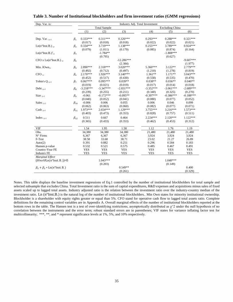
35
Table 3. Number of Institutional blockholders and firm investment ratios (GMM regressions)
Dep. Var. is: Industry Adj. Total Investment
Total Sample Excluding China
(1) (2) (3) (4) (5) (6)
Dep. Var. i,t-1 𝛽1 0.333*** 0.311*** 0.326*** 0.293*** 0.288*** 0.321***
(0.017) (0.018) (0.018) (0.022) (0.022) (0.021)
Ln(n°Inst.B.) i,t 𝛽2 0.334*** 3.719*** 1.138*** 0.255*** 3.789*** 0.924***
(0.079) (1.011) (0.179) (0.085) (0.874) (0.164)
Ln(n°Inst.B.)2i,t 𝛽3 -1.784** -1.808***
(0.795) (0.627)
CFO x Ln(n°Inst.B.) i,t 𝛽4 -12.286*** -9.607***
(2.384) (1.977)
Min. IOwni,t 𝛽5 2.890*** 2.318*** 3.020*** 5.360*** 3.122** 2.779***
(0.492) (0.712) (0.497) (1.210) (1.278) (0.819)
CFO i,t 𝛽6 2.170*** 1.926*** 3.140*** 1.361** 1.171** 3.043***
(0.452) (0.517) (0.430) (0.558) (0.535) (0.470)
Tobin's Q i,t-1 𝛽7 0.067*** 0.095*** 0.039** 0.038** 0.036** 0.040**
(0.019) (0.021) (0.019) (0.017) (0.014) (0.018)
Debt i,t-1 𝛽8 -3.218*** -3.347*** -2.831*** -3.352*** -3.061*** -2.689***
(0.239) (0.255) (0.211) (0.340) (0.325) (0.270)
Size i,t-1 𝛽9 -0.061 -0.172*** -0.095** -0.397*** -0.386*** -0.188***
(0.040) (0.052) (0.041) (0.080) (0.077) (0.052)
Sales i,t-1 𝛽10 -0.006 0.006 0.055 0.006 0.046 0.099
(0.062) (0.063) (0.060) (0.082) (0.077) (0.071)
Cash i,t-1 𝛽11 1.973*** 2.654*** 1.129*** 3.755*** 3.216*** 1.573***
(0.403) (0.473) (0.353) (0.828) (0.757) (0.511)
Index i,t-1 𝛽12 0.511 0.667 0.464 2.224*** 2.120*** 1.122***
(0.365) (0.433) (0.353) (0.462) (0.453) (0.312)
VIF 1.54 1.95 1.58 1.12 1.76 1.19
Obs. 34,380 34,380 34,380 21,480 21,480 21,480
N° Firms 6,367 6,367 6,367 3,924 3,924 3,924
F-Test 38.58 33.68 38.71 23.02 21.27 26.89 Auto(2) 0.391 0.882 0.251 0.296 0.584 0.183
Hansen p-value 0.532 0.521 0.575 0.485 0.467 0.491 Country-Year FE YES YES YES YES YES YES
Industry FE YES YES YES YES YES YES
Marginal Effect
(𝜕𝐼𝑛𝑣/𝜕Ln(n°Inst. B. ))=0 1.043*** 1.048***
(0.203) (0.149)
𝛽5 + 𝛽3 ∗ Ln(n°Inst. B. ) 0.549** 0.400
(0.261) (0.329)
Notes. This table displays the baseline investment regressions of Eq.1 controlled by the number of institutional blockholders for total sample and
selected subsample that excludes China. Total Investment ratio is the sum of capital expenditures, R&D expenses and acquisitions minus sales of fixed
assets scaled up to lagged total assets. Industry adjusted ratio is the relation between the investment ratio over the industry-country median of the
investment ratio. Ln (n°Inst.B.) is the natural log of the number of institutional blockholders.. Min Own states for minority institutional ownership.
Blockholder is a shareholder with equity rights greater or equal than 5%. CFO stand for operative cash flow to lagged total assets ratio. Complete
definitions for the remaining control variables are in Appendix A. Overall marginal effects of the number of institutional blockholders reported at the
bottom rows in the table. The Hansen test is a test of over-identifying restrictions, asymptotically distributed as χ^2 under the null hypothesis of no
correlation between the instruments and the error term; robust standard errors are in parentheses; VIF states for variance inflating factor test for
multicollinearity; ***, **, and * represent significance levels at 1%, 5%, and 10% respectively.
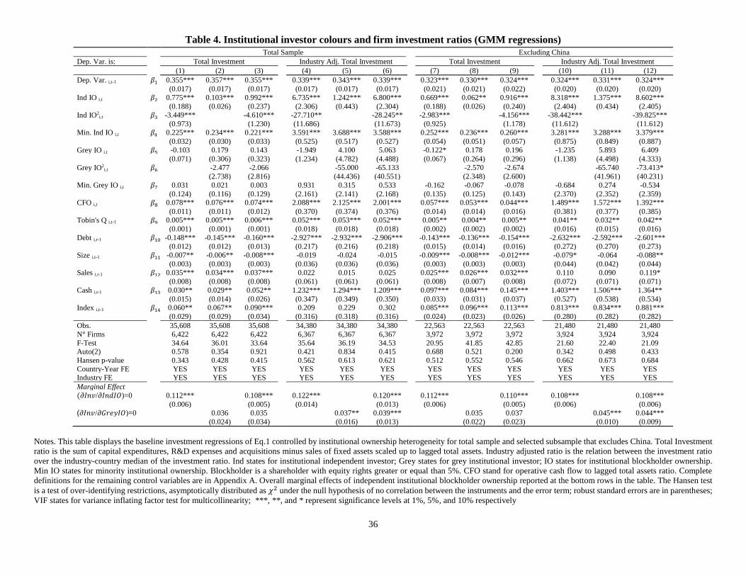
36
Table 4. Institutional investor colours and firm investment ratios (GMM regressions)
Total Sample Excluding China
Dep. Var. is: Total Investment Industry Adj. Total Investment Total Investment Industry Adj. Total Investment
(1) (2) (3) (4) (5) (6) (7) (8) (9) (10) (11) (12)
Dep. Var. i,t-1 𝛽1 0.355*** 0.357*** 0.355*** 0.339*** 0.343*** 0.339*** 0.323*** 0.330*** 0.324*** 0.324*** 0.331*** 0.324***
(0.017) (0.017) (0.017) (0.017) (0.017) (0.017) (0.021) (0.021) (0.022) (0.020) (0.020) (0.020)
Ind IO i,t 𝛽2 0.775*** 0.103*** 0.992*** 6.735*** 1.242*** 6.800*** 0.669*** 0.062** 0.916*** 8.318*** 1.375*** 8.602***
(0.188) (0.026) (0.237) (2.306) (0.443) (2.304) (0.188) (0.026) (0.240) (2.404) (0.434) (2.405)
Ind IO2i,t 𝛽3 -3.449*** -4.610*** -27.710** -28.245** -2.983*** -4.156*** -38.442*** -39.825***
(0.973) (1.230) (11.686) (11.673) (0.925) (1.178) (11.612) (11.612)
Min. Ind IO i,t 𝛽4 0.225*** 0.234*** 0.221*** 3.591*** 3.688*** 3.588*** 0.252*** 0.236*** 0.260*** 3.281*** 3.288*** 3.379***
(0.032) (0.030) (0.033) (0.525) (0.517) (0.527) (0.054) (0.051) (0.057) (0.875) (0.849) (0.887)
Grey IO i,t 𝛽5 -0.103 0.179 0.143 -1.949 4.100 5.063 -0.122* 0.178 0.196 -1.235 5.893 6.409
(0.071) (0.306) (0.323) (1.234) (4.782) (4.488) (0.067) (0.264) (0.296) (1.138) (4.498) (4.333)
Grey IO2i,t 𝛽6 -2.477 -2.066 -55.000 -65.133 -2.570 -2.674 -65.740 -73.413*
(2.738) (2.816) (44.436) (40.551) (2.348) (2.600) (41.961) (40.231)
Min. Grey IO i,t 𝛽7 0.031 0.021 0.003 0.931 0.315 0.533 -0.162 -0.067 -0.078 -0.684 0.274 -0.534
(0.124) (0.116) (0.129) (2.161) (2.141) (2.168) (0.135) (0.125) (0.143) (2.370) (2.352) (2.359)
CFO i,t 𝛽8 0.078*** 0.076*** 0.074*** 2.088*** 2.125*** 2.001*** 0.057*** 0.053*** 0.044*** 1.489*** 1.572*** 1.392***
(0.011) (0.011) (0.012) (0.370) (0.374) (0.376) (0.014) (0.014) (0.016) (0.381) (0.377) (0.385)
Tobin's Q i,t-1 𝛽9 0.005*** 0.005*** 0.006*** 0.052*** 0.053*** 0.052*** 0.005** 0.004** 0.005** 0.041** 0.032** 0.042**
(0.001) (0.001) (0.001) (0.018) (0.018) (0.018) (0.002) (0.002) (0.002) (0.016) (0.015) (0.016)
Debt i,t-1 𝛽10 -0.148*** -0.145*** -0.160*** -2.927*** -2.932*** -2.906*** -0.143*** -0.136*** -0.154*** -2.632*** -2.592*** -2.601***
(0.012) (0.012) (0.013) (0.217) (0.216) (0.218) (0.015) (0.014) (0.016) (0.272) (0.270) (0.273)
Size i,t-1 𝛽11 -0.007** -0.006** -0.008*** -0.019 -0.024 -0.015 -0.009*** -0.008*** -0.012*** -0.079* -0.064 -0.088**
(0.003) (0.003) (0.003) (0.036) (0.036) (0.036) (0.003) (0.003) (0.003) (0.044) (0.042) (0.044)
Sales i,t-1 𝛽12 0.035*** 0.034*** 0.037*** 0.022 0.015 0.025 0.025*** 0.026*** 0.032*** 0.110 0.090 0.119*
(0.008) (0.008) (0.008) (0.061) (0.061) (0.061) (0.008) (0.007) (0.008) (0.072) (0.071) (0.071)
Cash i,t-1 𝛽13 0.030** 0.029** 0.052** 1.232*** 1.294*** 1.209*** 0.097*** 0.084*** 0.145*** 1.403*** 1.506*** 1.364**
(0.015) (0.014) (0.026) (0.347) (0.349) (0.350) (0.033) (0.031) (0.037) (0.527) (0.538) (0.534)
Index i,t-1 𝛽14 0.060** 0.067** 0.090*** 0.209 0.229 0.302 0.085*** 0.096*** 0.113*** 0.813*** 0.834*** 0.881***
(0.029) (0.029) (0.034) (0.316) (0.318) (0.316) (0.024) (0.023) (0.026) (0.280) (0.282) (0.282)
Obs. 35,608 35,608 35,608 34,380 34,380 34,380 22,563 22,563 22,563 21,480 21,480 21,480
N° Firms 6,422 6,422 6,422 6,367 6,367 6,367 3,972 3,972 3,972 3,924 3,924 3,924
F-Test 34.64 36.01 33.64 35.64 36.19 34.53 20.95 41.85 42.85 21.60 22.40 21.09 Auto(2) 0.578 0.354 0.921 0.421 0.834 0.415 0.688 0.521 0.200 0.342 0.498 0.433
Hansen p-value 0.343 0.428 0.415 0.562 0.613 0.621 0.512 0.552 0.546 0.662 0.673 0.684
Country-Year FE YES YES YES YES YES YES YES YES YES YES YES YES Industry FE YES YES YES YES YES YES YES YES YES YES YES YES
Marginal Effect
(𝜕𝐼𝑛𝑣/𝜕𝐼𝑛𝑑𝐼𝑂)=0 0.112*** 0.108*** 0.122*** 0.120*** 0.112*** 0.110*** 0.108*** 0.108***
(0.006) (0.005) (0.014) (0.013) (0.006) (0.005) (0.006) (0.006)
(𝜕𝐼𝑛𝑣/𝜕𝐺𝑟𝑒𝑦𝐼𝑂)=0 0.036 0.035 0.037** 0.039*** 0.035 0.037 0.045*** 0.044***
(0.024) (0.034) (0.016) (0.013) (0.022) (0.023) (0.010) (0.009)
Notes. This table displays the baseline investment regressions of Eq.1 controlled by institutional ownership heterogeneity for total sample and selected subsample that excludes China. Total Investment
ratio is the sum of capital expenditures, R&D expenses and acquisitions minus sales of fixed assets scaled up to lagged total assets. Industry adjusted ratio is the relation between the investment ratio
over the industry-country median of the investment ratio. Ind states for institutional independent investor; Grey states for grey institutional investor; IO states for institutional blockholder ownership.
Min IO states for minority institutional ownership. Blockholder is a shareholder with equity rights greater or equal than 5%. CFO stand for operative cash flow to lagged total assets ratio. Complete
definitions for the remaining control variables are in Appendix A. Overall marginal effects of independent institutional blockholder ownership reported at the bottom rows in the table. The Hansen test
is a test of over-identifying restrictions, asymptotically distributed as 𝜒2 under the null hypothesis of no correlation between the instruments and the error term; robust standard errors are in parentheses;
VIF states for variance inflating factor test for multicollinearity; ***, **, and * represent significance levels at 1%, 5%, and 10% respectively
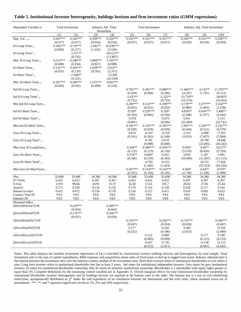
37
Table 5. Institutional Investor heterogeneity, holdings horizon and firm investment ratios (GMM regressions)
Dependent Variable is: Total Investment Industry Adj. Total
Investment
Total Investment Industry Adj. Total Investment
(1) (2) (3) (4) (5) (6) (7) (8) (9) (10)
Dep. Var. i,t-1 0.347*** 0.342*** 0.328*** 0.324*** 0.352*** 0.351*** 0.351*** 0.330*** 0.331*** 0.328***
(0.017) (0.017) (0.018) (0.018) (0.017) (0.017) (0.017) (0.018) (0.018) (0.018)
IO-Long Term i,t 0.266*** 0.719*** 2.941** 10.630*** (0.069) (0.217) (1.225) (3.520)
IO-Long Term2 i,t -1.571** -26.512**
(0.735) (12.807) Min. IO-Long Term i,t 0.213*** 0.246*** 2.884*** 3.195***
(0.048) (0.054) (0.827) (0.888)
IO-Short Term i,t 0.131*** 0.365*** 1.639*** 5.023** (0.031) (0.120) (0.561) (2.371)
IO-Short Term2 i,t -1.048** -15.305
(0.521) (10.159) Min. IO-Short Term i,t 0.207*** 0.200*** 3.121*** 3.063***
(0.029) (0.032) (0.499) (0.519)
Ind IO-Long Term i,t 0.702*** 0.281*** 0.688*** 11.460*** 4.133** 11.276*** (0.204) (0.084) (0.206) (4.247) (1.791) (4.312)
Ind IO-Long Term2 i,t -1.623** -1.525** -33.718** -30.693*
(0.722) (0.725) (16.374) (16.453) Min.Ind IO-Long Term i,t 0.200*** 0.214*** 0.208*** 3.179*** 3.377*** 3.354***
(0.051) (0.051) (0.052) (0.989) (1.003) (1.038)
Ind IO-Short Term i,t 0.319* 0.220*** 0.326* 4.839** 6.634*** 5.408** (0.193) (0.085) (0.169) (2.248) (1.977) (2.642)
Ind IO-Short Term2 i,t -0.576 -0.672 5.031 5.115
(0.801) (0.836) (22.409) (22.741) Min.Ind IO-Short Term i,t 0.195*** 0.193*** 0.195*** 3.305*** 3.224*** 3.332***
(0.029) (0.029) (0.029) (0.564) (0.551) (0.579)
Grey IO-Long Term i,t 0.074 -0.167 -0.120 -2.311 -6.998 -7.103 (0.101) (0.262) (0.249) (3.933) (7.657) (7.904)
Grey IO-Long Term2 i,t 0.745 0.679 19.790 18.648
(0.898) (0.848) (25.005) (26.342) Min Grey IO LongTerm i,t 0.304** 0.384*** 0.334*** 9.050* 4.387* 10.277*
(0.122) (0.123) (0.126) (5.533) (8.426) (5.520)
Grey IO-Short Term i,t 0.374** 0.669* 0.455 3.850 5.187 3.991 (0.186) (0.370) (0.365) (10.606) (11.207) (11.313)
Grey IO-Short Term2 i,t -0.765 -0.313 18.731 17.656
(1.442) (1.423) (55.323) (54.354)
Min Grey IO ShortTerm i,t 0.307*** 0.314*** 0.324*** 4.504* 4.447* 4.970*
(0.101) (0.104) (0.105) (2.730) (2.358) (2.999)
Obs. 35,608 35,608 34,380 34,380 35,608 35,608 35,608 34,380 34,380 34,380 N° Firms 6,422 6,422 6,367 6,367 6,422 6,422 6,422 6,367 6,367 6,367
F-Test 119.9 98.84 34.93 31.37 32.40 113.6 105.7 26.65 27.66 25.44
Auto(2) 0.175 0.258 0.134 0.153 0.170 0.110 0.158 0.250 0.117 0.242 Hansen p-value 0.415 0.472 0.554 0.576 0.316 0.372 0.411 0.616 0.605 0.633
Country-Year FE YES YES YES YES YES YES YES YES YES YES
Industry FE YES YES YES YES YES YES YES YES YES YES
Marginal Effect
(𝜕𝐼𝑛𝑣/𝜕𝐼𝑂𝑤𝑛𝐿𝑇)=0 0.229*** 0.200***
(0.050) (0.043)
(𝜕𝐼𝑛𝑣/𝜕𝐼𝑂𝑤𝑛𝑆𝑇)=0 0.174*** 0.164***
(0.037) (0.039)
(𝜕𝐼𝑛𝑣/𝜕𝐼𝑛𝑑𝐼𝑂𝐿𝑇)=0 0.216*** 0.226*** 0.170*** 0.184***
(0.047) (0.054) (0.038) (0.047)
(𝜕𝐼𝑛𝑣/𝜕𝐼𝑛𝑑𝐼𝑂𝑆𝑇)=0 0.277 0.242 -0.481 -0.529
(0.252) (0.186) (2.633) (2.840)
(𝜕𝐼𝑛𝑣/𝜕𝐺𝑟𝑒𝑦𝐼𝑂𝐿𝑇)=0 0.112 0.089 0.177 0.190
(0.083) (0.099) (0.115) (0.133)
(𝜕𝐼𝑛𝑣/𝜕𝐺𝑟𝑒𝑦𝐼𝑂𝑆𝑇)=0 0.437 0.726 -0.138 -0.113
(0.622) (2.811) (0.681) (0.642)
Notes. This table displays the baseline investment regressions of Eq.1 controlled by institutional investor holdings horizon and heterogeneity for total sample. Total Investment ratio is the sum of capital expenditures, R&D expenses and acquisitions minus sales of fixed assets scaled up to lagged total assets. Industry adjusted ratio is
the relation between the investment ratio over the industry-country median of the investment ratio. Short term investor refers to institutional shareholders to exit within a
year; Long term investor refers to institutional shareholder that last at least 2 years; Ind states for institutional independent investor; Grey states for grey institutional investor; IO states for institutional blockholder ownership. Min IO states for minority institutional ownership. Blockholder is a shareholder with equity rights greater or
equal than 5%. Complete definitions for the remaining control variables are in Appendix A. Overall marginal effects for total institutional blockholder ownership by
institutional blockholder investor heterogeneity and by holdings horizon are reported at the bottom rows in the table. The Hansen test is a test of over-identifying
restrictions, asymptotically distributed as 𝜒2 under the null hypothesis of no correlation between the instruments and the error term; robust standard errors are in
parentheses; ***, **, and * represent significance levels at 1%, 5%, and 10% respectively.
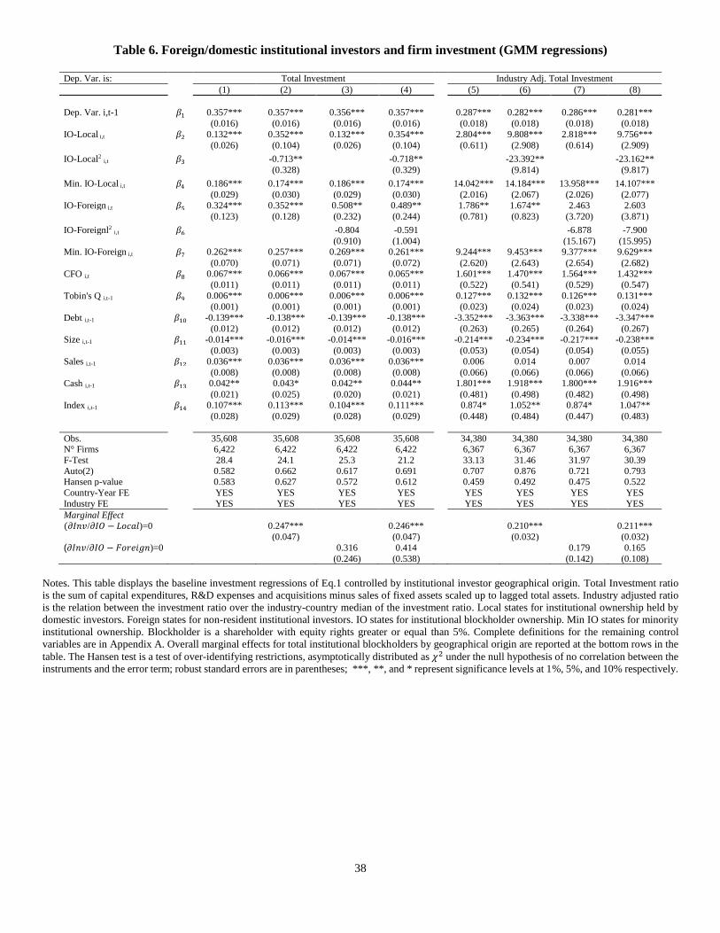
38
Table 6. Foreign/domestic institutional investors and firm investment (GMM regressions)
Dep. Var. is: Total Investment Industry Adj. Total Investment
(1) (2) (3) (4) (5) (6) (7) (8)
Dep. Var. i,t-1 𝛽1 0.357*** 0.357*** 0.356*** 0.357*** 0.287*** 0.282*** 0.286*** 0.281***
(0.016) (0.016) (0.016) (0.016) (0.018) (0.018) (0.018) (0.018)
IO-Local i,t 𝛽2 0.132*** 0.352*** 0.132*** 0.354*** 2.804*** 9.808*** 2.818*** 9.756***
(0.026) (0.104) (0.026) (0.104) (0.611) (2.908) (0.614) (2.909)
IO-Local2 i,t 𝛽3 -0.713** -0.718** -23.392** -23.162**
(0.328) (0.329) (9.814) (9.817)
Min. IO-Local i,t 𝛽4 0.186*** 0.174*** 0.186*** 0.174*** 14.042*** 14.184*** 13.958*** 14.107***
(0.029) (0.030) (0.029) (0.030) (2.016) (2.067) (2.026) (2.077)
IO-Foreign i,t 𝛽5 0.324*** 0.352*** 0.508** 0.489** 1.786** 1.674** 2.463 2.603
(0.123) (0.128) (0.232) (0.244) (0.781) (0.823) (3.720) (3.871)
IO-Foreignl2 i,t 𝛽6 -0.804 -0.591 -6.878 -7.900
(0.910) (1.004) (15.167) (15.995) Min. IO-Foreign i,t 𝛽7 0.262*** 0.257*** 0.269*** 0.261*** 9.244*** 9.453*** 9.377*** 9.629***
(0.070) (0.071) (0.071) (0.072) (2.620) (2.643) (2.654) (2.682)
CFO i,t 𝛽8 0.067*** 0.066*** 0.067*** 0.065*** 1.601*** 1.470*** 1.564*** 1.432***
(0.011) (0.011) (0.011) (0.011) (0.522) (0.541) (0.529) (0.547)
Tobin's Q i,t-1 𝛽9 0.006*** 0.006*** 0.006*** 0.006*** 0.127*** 0.132*** 0.126*** 0.131***
(0.001) (0.001) (0.001) (0.001) (0.023) (0.024) (0.023) (0.024)
Debt i,t-1 𝛽10 -0.139*** -0.138*** -0.139*** -0.138*** -3.352*** -3.363*** -3.338*** -3.347***
(0.012) (0.012) (0.012) (0.012) (0.263) (0.265) (0.264) (0.267)
Size i,t-1 𝛽11 -0.014*** -0.016*** -0.014*** -0.016*** -0.214*** -0.234*** -0.217*** -0.238***
(0.003) (0.003) (0.003) (0.003) (0.053) (0.054) (0.054) (0.055)
Sales i,t-1 𝛽12 0.036*** 0.036*** 0.036*** 0.036*** 0.006 0.014 0.007 0.014
(0.008) (0.008) (0.008) (0.008) (0.066) (0.066) (0.066) (0.066)
Cash i,t-1 𝛽13 0.042** 0.043* 0.042** 0.044** 1.801*** 1.918*** 1.800*** 1.916***
(0.021) (0.025) (0.020) (0.021) (0.481) (0.498) (0.482) (0.498)
Index i,t-1 𝛽14 0.107*** 0.113*** 0.104*** 0.111*** 0.874* 1.052** 0.874* 1.047**
(0.028) (0.029) (0.028) (0.029) (0.448) (0.484) (0.447) (0.483)
Obs. 35,608 35,608 35,608 35,608 34,380 34,380 34,380 34,380 N° Firms 6,422 6,422 6,422 6,422 6,367 6,367 6,367 6,367
F-Test 28.4 24.1 25.3 21.2 33.13 31.46 31.97 30.39
Auto(2) 0.582 0.662 0.617 0.691 0.707 0.876 0.721 0.793 Hansen p-value 0.583 0.627 0.572 0.612 0.459 0.492 0.475 0.522
Country-Year FE YES YES YES YES YES YES YES YES
Industry FE YES YES YES YES YES YES YES YES
Marginal Effect
(𝜕𝐼𝑛𝑣/𝜕𝐼𝑂 − 𝐿𝑜𝑐𝑎𝑙)=0 0.247*** 0.246*** 0.210*** 0.211***
(0.047) (0.047) (0.032) (0.032)
(𝜕𝐼𝑛𝑣/𝜕𝐼𝑂 − 𝐹𝑜𝑟𝑒𝑖𝑔𝑛)=0 0.316 0.414 0.179 0.165
(0.246) (0.538) (0.142) (0.108)
Notes. This table displays the baseline investment regressions of Eq.1 controlled by institutional investor geographical origin. Total Investment ratio
is the sum of capital expenditures, R&D expenses and acquisitions minus sales of fixed assets scaled up to lagged total assets. Industry adjusted ratio
is the relation between the investment ratio over the industry-country median of the investment ratio. Local states for institutional ownership held by
domestic investors. Foreign states for non-resident institutional investors. IO states for institutional blockholder ownership. Min IO states for minority
institutional ownership. Blockholder is a shareholder with equity rights greater or equal than 5%. Complete definitions for the remaining control
variables are in Appendix A. Overall marginal effects for total institutional blockholders by geographical origin are reported at the bottom rows in the
table. The Hansen test is a test of over-identifying restrictions, asymptotically distributed as 𝜒2 under the null hypothesis of no correlation between the
instruments and the error term; robust standard errors are in parentheses; ***, **, and * represent significance levels at 1%, 5%, and 10% respectively.
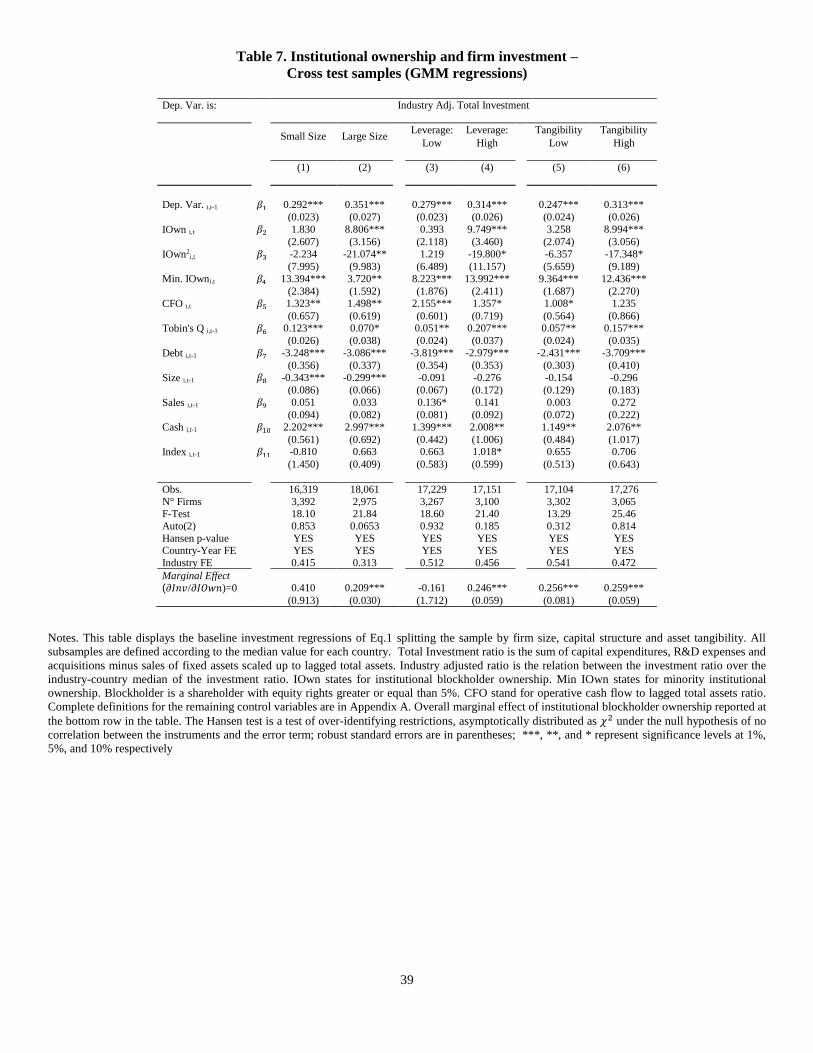
39
Table 7. Institutional ownership and firm investment –
Cross test samples (GMM regressions)
Dep. Var. is: Industry Adj. Total Investment
Small Size Large Size
Leverage:
Low
Leverage:
High
Tangibility
Low
Tangibility
High
(1) (2) (3) (4) (5) (6)
Dep. Var. i,t-1 𝛽1 0.292*** 0.351*** 0.279*** 0.314*** 0.247*** 0.313***
(0.023) (0.027) (0.023) (0.026) (0.024) (0.026)
IOwn i,t 𝛽2 1.830 8.806*** 0.393 9.749*** 3.258 8.994***
(2.607) (3.156) (2.118) (3.460) (2.074) (3.056)
IOwn2i,t 𝛽3 -2.234 -21.074** 1.219 -19.800* -6.357 -17.348*
(7.995) (9.983) (6.489) (11.157) (5.659) (9.189)
Min. IOwni,t 𝛽4 13.394*** 3.720** 8.223*** 13.992*** 9.364*** 12.436***
(2.384) (1.592) (1.876) (2.411) (1.687) (2.270)
CFO i,t 𝛽5 1.323** 1.498** 2.155*** 1.357* 1.008* 1.235
(0.657) (0.619) (0.601) (0.719) (0.564) (0.866)
Tobin's Q i,t-1 𝛽6 0.123*** 0.070* 0.051** 0.207*** 0.057** 0.157***
(0.026) (0.038) (0.024) (0.037) (0.024) (0.035)
Debt i,t-1 𝛽7 -3.248*** -3.086*** -3.819*** -2.979*** -2.431*** -3.709***
(0.356) (0.337) (0.354) (0.353) (0.303) (0.410)
Size i,t-1 𝛽8 -0.343*** -0.299*** -0.091 -0.276 -0.154 -0.296
(0.086) (0.066) (0.067) (0.172) (0.129) (0.183)
Sales i,t-1 𝛽9 0.051 0.033 0.136* 0.141 0.003 0.272
(0.094) (0.082) (0.081) (0.092) (0.072) (0.222)
Cash i,t-1 𝛽10 2.202*** 2.997*** 1.399*** 2.008** 1.149** 2.076**
(0.561) (0.692) (0.442) (1.006) (0.484) (1.017)
Index i,t-1 𝛽11 -0.810 0.663 0.663 1.018* 0.655 0.706
(1.450) (0.409) (0.583) (0.599) (0.513) (0.643)
Obs. 16,319 18,061 17,229 17,151 17,104 17,276
N° Firms 3,392 2,975 3,267 3,100 3,302 3,065 F-Test 18.10 21.84 18.60 21.40 13.29 25.46
Auto(2) 0.853 0.0653 0.932 0.185 0.312 0.814
Hansen p-value YES YES YES YES YES YES Country-Year FE YES YES YES YES YES YES
Industry FE 0.415 0.313 0.512 0.456 0.541 0.472
Marginal Effect
(𝜕𝐼𝑛𝑣/𝜕𝐼𝑂𝑤𝑛)=0 0.410 0.209*** -0.161 0.246*** 0.256*** 0.259***
(0.913) (0.030) (1.712) (0.059) (0.081) (0.059)
Notes. This table displays the baseline investment regressions of Eq.1 splitting the sample by firm size, capital structure and asset tangibility. All
subsamples are defined according to the median value for each country. Total Investment ratio is the sum of capital expenditures, R&D expenses and
acquisitions minus sales of fixed assets scaled up to lagged total assets. Industry adjusted ratio is the relation between the investment ratio over the
industry-country median of the investment ratio. IOwn states for institutional blockholder ownership. Min IOwn states for minority institutional
ownership. Blockholder is a shareholder with equity rights greater or equal than 5%. CFO stand for operative cash flow to lagged total assets ratio.
Complete definitions for the remaining control variables are in Appendix A. Overall marginal effect of institutional blockholder ownership reported at
the bottom row in the table. The Hansen test is a test of over-identifying restrictions, asymptotically distributed as 𝜒2 under the null hypothesis of no
correlation between the instruments and the error term; robust standard errors are in parentheses; ***, **, and * represent significance levels at 1%,
5%, and 10% respectively
40
Table 8. Institutional ownership and investment-cash flow sensitivity
Cross test samples (GMM regressions)
Dep. Var. is: Industry Adj. Total Investment
Small Size Large Size
Leverage:
Low
Leverage:
High
Tangibility
Low
Tangibility
High
(1) (2) (3) (4) (5) (6)
Dep. Var. i,t-1 𝛽1 0.312*** 0.397*** 0.298*** 0.484*** 0.278*** 0.467***
(0.022) (0.024) (0.022) (0.024) (0.023) (0.022)
IOwn i,t 𝛽2 2.531*** 3.165*** 1.716** 0.034 2.646*** 1.084
(0.898) (0.645) (0.708) (0.701) (0.677) (0.823)
CFO x IOwn i,t 𝛽3 -23.150** -23.265*** -16.258** -6.360 -25.847*** 13.028
(10.741) (7.881) (6.600) (9.397) (7.897) (9.057)
Min. IOwn i,t 𝛽4 2.179*** 1.909*** 1.632*** 2.522*** 2.061*** 1.705**
(0.679) (0.574) (0.607) (0.707) (0.508) (0.724)
CFO i,t 𝛽5 2.204*** 2.451*** 2.835*** 3.919*** 1.902*** 3.755***
(0.653) (0.579) (0.534) (0.647) (0.468) (0.668)
Tobin's Q i,t-1 𝛽6 0.048** 0.063** 0.042** 0.089*** 0.031* 0.047**
(0.020) (0.026) (0.017) (0.024) (0.018) (0.023)
Debt i,t-1 𝛽7 -2.914*** -2.335*** -3.320*** -2.755*** -2.003*** -2.533***
(0.316) (0.282) (0.312) (0.398) (0.254) (0.306)
Size i,t-1 𝛽8 -0.156** -0.214*** -0.011 -0.034 -0.004 -0.023
(0.072) (0.051) (0.051) (0.024) (0.042) (0.024)
Sales i,t-1 𝛽9 0.149* 0.042 0.083 0.046 0.040 0.043
(0.085) (0.070) (0.076) (0.056) (0.062) (0.064)
Cash i,t-1 𝛽10 1.143*** 2.253*** 0.847** 1.968*** 1.133*** 1.274**
(0.431) (0.517) (0.365) (0.617) (0.364) (0.612)
Index i,t-1 𝛽11 0.059 0.551** 0.040 0.015 0.290 0.782
(0.699) (0.255) (0.482) (0.309) (0.384) (0.559)
Obs. 16,319 18,061 17,229 17,151 17,104 17,276
N° Firms 3,392 2,975 3,267 3,100 3,302 3,065
F-Test 19.16 27.55 21.50 32.23 17.22 39.62 Auto(2) 0.251 0.816 0.397 0.307 0.807 0.683
Hansen p-value 0.622 0.714 0.734 0.685 0.553 0.526
Country-Year FE YES YES YES YES YES YES Industry FE YES YES YES YES YES YES
Marginal Effect
𝛽6 + 𝛽4 ∗ 𝐼𝑂𝑤𝑛 1.678*** 1.444*** 2.254*** 3.720*** 1.009** 4.178***
(0.549) (0.484) (0.474) (0.569) (0.408) (0.648)
Notes. This table displays the baseline investment regressions of Eq.1 splitting the sample by firm size, capital structure and asset tangibility. All
subsamples are defined according to the median value for each country. Total Investment ratio is the sum of capital expenditures, R&D expenses and
acquisitions minus sales of fixed assets scaled up to lagged total assets. Industry adjusted ratio is the relation between the investment ratio over the
industry-country median of the investment ratio. IOwn states for institutional blockholder ownership. Min IOwn states for minority institutional
ownership. Blockholder is a shareholder with equity rights greater or equal than 5%. CFO stand for operative cash flow to lagged total assets ratio.
Complete definitions for the remaining control variables are in Appendix A. Overall marginal effect of CFO is reported at the bottom row in the table.
The Hansen test is a test of over-identifying restrictions, asymptotically distributed as 𝜒2 under the null hypothesis of no correlation between the
instruments and the error term; robust standard errors are in parentheses; ***, **, and * represent significance levels at 1%, 5%, and 10% respectively
41
Table 9. Institutional ownership, country corporate governance and firm investment (GMM regressions) Dep. Var. is: Industry Adj. Total Investment
X i,t is: Regulatory Quality Rule of Law Civil Law Dummy
(1) (2) (3) (4) (5) (6) (7) (8) (9)
Dep. Var. i,t-1 𝛽1 0.367*** 0.347*** 0.333*** 0.359*** 0.357*** 0.337*** 0.376*** 0.377*** 0.335***
(0.018) (0.019) (0.016) (0.019) (0.019) (0.017) (0.026) (0.026) (0.017)
IOwn i,t 𝛽2 10.934*** 9.950** 4.488*** 5.665** 6.819** 4.019*** 8.130** 7.504* 4.139***
(3.702) (4.281) (1.203) (2.525) (2.857) (0.864) (3.799) (3.866) (0.862)
IOwn i,t * X i,t 𝛽3 -2.375 3.734 -2.121 -4.924 -2.100 -1.613 11.828 11.976 1.016
(4.803) (6.333) (2.006) (3.423) (3.896) (1.643) (9.736) (9.772) (1.195)
IOwn2i,t 𝛽4 -23.138** -23.966** -15.208** -21.326** -25.830*** -23.631**
(10.649) (12.071) (7.632) (8.746) (9.767) (9.974)
IOwn2i,t * X i,t 𝛽5 11.722 5.361 14.374 9.253 -16.482 -18.497
(12.762) (17.904) (9.757) (11.573) (26.174) (26.472)
Min. IOwni,t 𝛽6 2.336*** 5.003*** 3.474*** 2.256*** 4.871*** 3.235*** 0.730 1.639 3.342***
(0.526) (0.889) (0.490) (0.507) (0.629) (0.491) (0.903) (1.149) (0.506)
Min. IOwni,t* X i,t 𝛽7 -13.878*** -12.863** -9.751
(3.171) (2.045) (6.814)
CFO i,t 𝛽8 1.956*** 2.227*** 2.623*** 2.854*** 3.137*** 1.982*** 3.621*** 3.658*** 1.327***
(0.466) (0.530) (0.447) (0.471) (0.486) (0.307) (0.588) (0.587) (0.354)
CFO i,t * IOwn i,t 𝛽9 -62.748*** -36.641*** -33.433***
(12.807) (9.511) (9.654)
CFO i,t * IOwn i,t* X i,t 𝛽10 68.345*** 34.724** -2.614
(17.398) (14.462) (17.641)
CFO i,t * X i,t 𝛽11 -3.178*** -1.746* 9.195***
(1.185) (1.033) (3.056)
Obs. 34,380 34,380 34,380 34,380 34,380 34,380 34,380 34,380 34,380
N° Firms 6,367 6,367 6,367 6,367 6,367 6,367 6,367 6,367 6,367
F-Test 32.93 29.99 37.68 30.92 29.54 35.46 20.48 20.16 34.84 Auto(2) 0.460 0.278 0.496 0.287 0.451 0.332 0.500 0.509 0.225
Hansen p-value 0.371 0.326 0.432 0.215 0.205 0.294 0.241 0. 236 0.428 Country-Year FE YES YES YES YES YES YES YES YES YES
Industry FE YES YES YES YES YES YES YES YES YES
Marginal Effect
𝛽2 + 𝛽3 ∗ X𝑖,𝑡 10.197*** 11.109*** 4.992** 6.532** 19.958** 19.479**
(2.912) (3.397) (2.343) (2.632) (8.983) (8.982)
𝛽4 + 𝛽5 ∗ X𝑖,𝑡 -19.500** -22.302** -13.245* -20.062** -42.312* -42.128*
(8.639) (10.062) (7.255) (8.237) (25.336) (25.482)
𝛽8 + 𝛽9 ∗ IOwn𝑖,𝑡 0.518 0.758** 0.210
(0.496) (0.295) (0.295)
𝛽8 + 𝛽9 ∗ IOwn𝑖,𝑡 + 𝛽10 ∗ IOwn𝑖,𝑡 ∗ X𝑖,𝑡 1.229*** 0.917*** 0.122
(0.438) (0.273) (0.651)
Notes: This table displays the baseline investment regressions of Eq.1 including the interacting term of a country’s corporate governance proxies with institutional ownership. Country’s investor
protection variables are regulatory quality, rule of law and civil law dummy. Total Investment ratio is the sum of capital expenditures, R&D expenses and acquisitions minus sales of fixed assets scaled
up to lagged total assets. Industry adjusted ratio is the relation between the investment ratio over the industry-country median of the investment ratio. IOwn states for institutional blockholder ownership.
Min IOwn states for minority institutional ownership. Blockholder is a shareholder with equity rights greater or equal than 5%. CFO stand for operative cash flow to lagged total assets ratio. Complete
definitions for the remaining control variables are in Appendix A. Overall marginal effects on country corporate governance variables are at the bottom rows in the table. The Hansen test is a test of
over-identifying restrictions, asymptotically distributed as 𝜒2 under the null hypothesis of no correlation between the instruments and the error term; robust standard errors are in parentheses; ***, **,
and * represent significance levels at 1%, 5%, and 10% respectively

42
APPENDIX
Appendix A. Variable definition
43
Appendix A. Variable definition (Cont.)
Sources: Firm level variables data from Thomson’s Eikon (Datatream) and S&P Capital IQ. Country level variables: Wold Bank -
WGI Indicators.
44
Appendix B. Descriptive statistics by country 2004-2016
(Mean values and standard deviation)
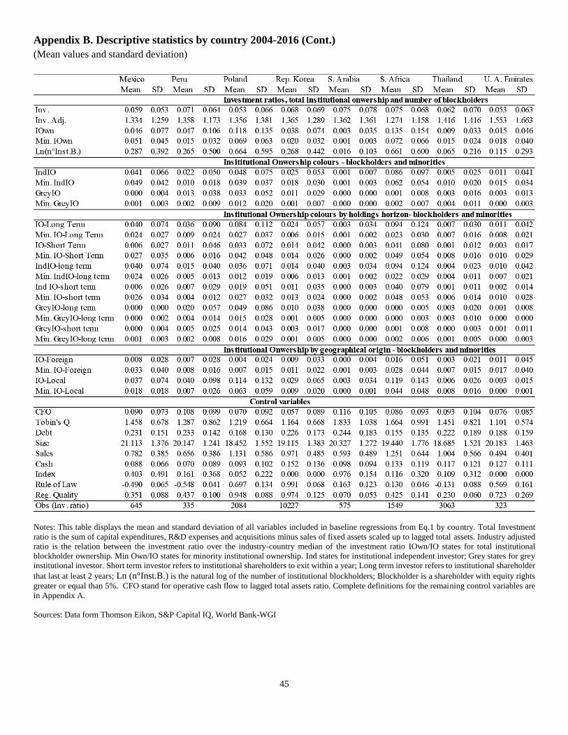
45
Appendix B. Descriptive statistics by country 2004-2016 (Cont.)
(Mean values and standard deviation)
Notes: This table displays the mean and standard deviation of all variables included in baseline regressions from Eq.1 by country. Total Investment
ratio is the sum of capital expenditures, R&D expenses and acquisitions minus sales of fixed assets scaled up to lagged total assets. Industry adjusted
ratio is the relation between the investment ratio over the industry-country median of the investment ratio IOwn/IO states for total institutional
blockholder ownership. Min Own/IO states for minority institutional ownership. Ind states for institutional independent investor; Grey states for grey
institutional investor. Short term investor refers to institutional shareholders to exit within a year; Long term investor refers to institutional shareholder
that last at least 2 years; Ln (n°Inst.B.) is the natural log of the number of institutional blockholders; Blockholder is a shareholder with equity rights
greater or equal than 5%. CFO stand for operative cash flow to lagged total assets ratio. Complete definitions for the remaining control variables are
in Appendix A.
Sources: Data form Thomson Eikon, S&P Capital IQ, World Bank-WGI
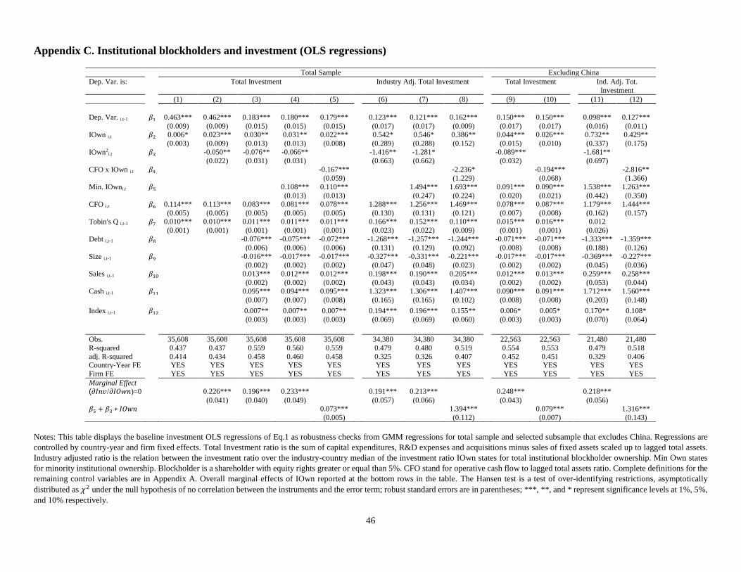
46
Appendix C. Institutional blockholders and investment (OLS regressions)
Total Sample Excluding China
Dep. Var. is: Total Investment Industry Adj. Total Investment Total Investment Ind. Adj. Tot.
Investment
(1) (2) (3) (4) (5) (6) (7) (8) (9) (10) (11) (12)
Dep. Var. i,t-1 𝛽1 0.463*** 0.462*** 0.183*** 0.180*** 0.179*** 0.123*** 0.121*** 0.162*** 0.150*** 0.150*** 0.098*** 0.127***
(0.009) (0.009) (0.015) (0.015) (0.015) (0.017) (0.017) (0.009) (0.017) (0.017) (0.016) (0.011)
IOwn i,t 𝛽2 0.006* 0.023*** 0.030** 0.031** 0.022*** 0.542* 0.546* 0.386** 0.044*** 0.026*** 0.732** 0.429**
(0.003) (0.009) (0.013) (0.013) (0.008) (0.289) (0.288) (0.152) (0.015) (0.010) (0.337) (0.175)
IOwn2i,t 𝛽3 -0.050** -0.076** -0.066** -1.416** -1.281* -0.089*** -1.681**
(0.022) (0.031) (0.031) (0.663) (0.662) (0.032) (0.697)
CFO x IOwn i,t 𝛽4 -0.167*** -2.236* -0.194*** -2.816**
(0.059) (1.229) (0.068) (1.366)
Min. IOwni,t 𝛽5 0.108*** 0.110*** 1.494*** 1.693*** 0.091*** 0.090*** 1.538*** 1.263***
(0.013) (0.013) (0.247) (0.224) (0.020) (0.021) (0.442) (0.350)
CFO i,t 𝛽6 0.114*** 0.113*** 0.083*** 0.081*** 0.078*** 1.288*** 1.256*** 1.469*** 0.078*** 0.087*** 1.179*** 1.444***
(0.005) (0.005) (0.005) (0.005) (0.005) (0.130) (0.131) (0.121) (0.007) (0.008) (0.162) (0.157)
Tobin's Q i,t-1 𝛽7 0.010*** 0.010*** 0.011*** 0.011*** 0.011*** 0.166*** 0.152*** 0.110*** 0.015*** 0.016*** 0.012
(0.001) (0.001) (0.001) (0.001) (0.001) (0.023) (0.022) (0.009) (0.001) (0.001) (0.026)
Debt i,t-1 𝛽8 -0.076*** -0.075*** -0.072*** -1.268*** -1.257*** -1.244*** -0.071*** -0.071*** -1.333*** -1.359***
(0.006) (0.006) (0.006) (0.131) (0.129) (0.092) (0.008) (0.008) (0.188) (0.126)
Size i,t-1 𝛽9 -0.016*** -0.017*** -0.017*** -0.327*** -0.331*** -0.221*** -0.017*** -0.017*** -0.369*** -0.227***
(0.002) (0.002) (0.002) (0.047) (0.048) (0.023) (0.002) (0.002) (0.045) (0.036)
Sales i,t-1 𝛽10 0.013*** 0.012*** 0.012*** 0.198*** 0.190*** 0.205*** 0.012*** 0.013*** 0.259*** 0.258***
(0.002) (0.002) (0.002) (0.043) (0.043) (0.034) (0.002) (0.002) (0.053) (0.044)
Cash i,t-1 𝛽11 0.095*** 0.094*** 0.095*** 1.323*** 1.306*** 1.407*** 0.090*** 0.091*** 1.712*** 1.560***
(0.007) (0.007) (0.008) (0.165) (0.165) (0.102) (0.008) (0.008) (0.203) (0.148)
Index i,t-1 𝛽12 0.007** 0.007** 0.007** 0.194*** 0.196*** 0.155** 0.006* 0.005* 0.170** 0.108*
(0.003) (0.003) (0.003) (0.069) (0.069) (0.060) (0.003) (0.003) (0.070) (0.064)
Obs. 35,608 35,608 35,608 35,608 35,608 34,380 34,380 34,380 22,563 22,563 21,480 21,480
R-squared 0.437 0.437 0.559 0.560 0.559 0.479 0.480 0.519 0.554 0.553 0.479 0.518
adj. R-squared 0.414 0.434 0.458 0.460 0.458 0.325 0.326 0.407 0.452 0.451 0.329 0.406 Country-Year FE YES YES YES YES YES YES YES YES YES YES YES YES
Firm FE YES YES YES YES YES YES YES YES YES YES YES YES
Marginal Effect
(𝜕𝐼𝑛𝑣/𝜕𝐼𝑂𝑤𝑛)=0 0.226*** 0.196*** 0.233*** 0.191*** 0.213*** 0.248*** 0.218***
(0.041) (0.040) (0.049) (0.057) (0.066) (0.043) (0.056)
𝛽5 + 𝛽3 ∗ 𝐼𝑂𝑤𝑛 0.073*** 1.394*** 0.079*** 1.316***
(0.005) (0.112) (0.007) (0.143)
Notes: This table displays the baseline investment OLS regressions of Eq.1 as robustness checks from GMM regressions for total sample and selected subsample that excludes China. Regressions are
controlled by country-year and firm fixed effects. Total Investment ratio is the sum of capital expenditures, R&D expenses and acquisitions minus sales of fixed assets scaled up to lagged total assets.
Industry adjusted ratio is the relation between the investment ratio over the industry-country median of the investment ratio IOwn states for total institutional blockholder ownership. Min Own states
for minority institutional ownership. Blockholder is a shareholder with equity rights greater or equal than 5%. CFO stand for operative cash flow to lagged total assets ratio. Complete definitions for the
remaining control variables are in Appendix A. Overall marginal effects of IOwn reported at the bottom rows in the table. The Hansen test is a test of over-identifying restrictions, asymptotically
distributed as 𝜒2 under the null hypothesis of no correlation between the instruments and the error term; robust standard errors are in parentheses; ***, **, and * represent significance levels at 1%, 5%,
and 10% respectively.
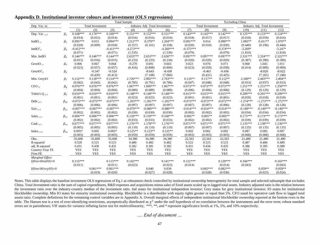
47
Appendix D. Institutional investor colours and investment (OLS regressions) Total Sample Excluding China
Dep. Var. is: Total Investment Industry Adj. Total Investment Total Investment Industry Adj. Total Investment
(1) (2) (3) (4) (5) (6) (7) (8) (9) (10) (11) (12)
Dep. Var. i,t-1 𝛽1 0.168*** 0.170*** 0.169*** 0.151*** 0.152*** 0.151*** 0.143*** 0.143*** 0.142*** 0.125*** 0.123*** 0.124***
(0.014) (0.015) (0.014) (0.016) (0.016) (0.016) (0.018) (0.017) (0.017) (0.018) (0.018) (0.016)
IndIO i,t 𝛽2 0.095*** 0.015 0.094*** 1.212*** 0.379** 1.204*** 0.091*** 0.014 0.090*** 1.083** 0.411** 1.070**
(0.018) (0.009) (0.018) (0.357) (0.161) (0.358) (0.020) (0.010) (0.020) (0.440) (0.196) (0.444)
IndIO2i,t 𝛽3 -0.412*** -0.411*** -4.273*** -4.260*** -0.375*** -0.374*** -3.269* -3.247*
(0.071) (0.071) (1.535) (1.539) (0.079) (0.079) (1.810) (1.818)
Min. IndIO 𝛽4 0.144*** 0.146*** 0.144*** 2.633*** 2.653*** 2.630*** 0.097*** 0.097*** 0.097*** 2.331*** 2.324*** 2.322***
(0.015) (0.016) (0.015) (0.233) (0.233) (0.234) (0.020) (0.020) (0.020) (0.387) (0.390) (0.389)
GreyIO i,t 𝛽5 0.006 0.067 0.064 -0.270 0.691 0.663 0.023 0.076 0.071 0.060 1.045 1.011
(0.023) (0.057) (0.057) (0.416) (0.898) (0.894) (0.023) (0.059) (0.058) (0.414) (0.909) (0.909)
GreyIO2i,t 𝛽6 -0.547 -0.524 -8.643 -8.438 -0.463 -0.436 -8.826 -8.622
(0.420) (0.413) (7.108) (7.060) (0.431) (0.425) (7.265) (7.248)
Min. GreyIO 𝛽7 0.112*** 0.118*** 0.114*** 2.726*** 2.802*** 2.763*** 0.110** 0.117** 0.112** 2.349** 2.443*** 2.404**
(0.042) (0.043) (0.042) (0.785) (0.791) (0.786) (0.047) (0.048) (0.048) (0.933) (0.937) (0.933)
CFO i,t 𝛽8 0.076*** 0.076*** 0.076*** 1.067*** 1.069*** 1.067*** 0.073*** 0.073*** 0.073*** 1.251*** 1.251*** 1.250***
(0.004) (0.004) (0.004) (0.089) (0.089) (0.089) (0.006) (0.006) (0.006) (0.129) (0.129) (0.129)
Tobin's Q i,t-1 𝛽9 0.010*** 0.010*** 0.010*** 0.148*** 0.149*** 0.148*** 0.015*** 0.015*** 0.015*** 0.200*** 0.201*** 0.200***
(0.001) (0.001) (0.001) (0.023) (0.023) (0.023) (0.001) (0.001) (0.001) (0.018) (0.018) (0.018)
Debt i,t-1 𝛽10 -0.075*** -0.075*** -0.075*** -1.203*** -1.201*** -1.202*** -0.073*** -0.073*** -0.072*** -1.274*** -1.273*** -1.272***
(0.006) (0.006) (0.006) (0.097) (0.097) (0.097) (0.007) (0.007) (0.006) (0.128) (0.128) (0.128)
Size i,t-1 𝛽11 -0.007*** -0.007*** -0.007*** -0.079*** -0.080*** -0.080*** -0.014*** -0.014*** -0.014*** -0.149*** -0.149*** -0.149***
(0.002) (0.002) (0.002) (0.030) (0.030) (0.030) (0.002) (0.002) (0.002) (0.034) (0.034) (0.034)
Sales i,t-1 𝛽12 0.006*** 0.006*** 0.006*** 0.159*** 0.159*** 0.160*** 0.005** 0.005** 0.005** 0.173*** 0.173*** 0.173***
(0.002) (0.002) (0.002) (0.033) (0.033) (0.033) (0.002) (0.002) (0.002) (0.039) (0.039) (0.039)
Cash i,t-1 𝛽13 0.077*** 0.077*** 0.077*** 1.176*** 1.178*** 1.176*** 0.071*** 0.071*** 0.071*** 1.135*** 1.138*** 1.136***
(0.005) (0.005) (0.005) (0.110) (0.110) (0.110) (0.007) (0.007) (0.007) (0.135) (0.135) (0.135)
Index i,t-1 𝛽14 0.005* 0.005 0.005* 0.125** 0.123** 0.125** 0.002 0.002 0.002 0.087 0.085 0.087
(0.003) (0.003) (0.003) (0.059) (0.059) (0.059) (0.003) (0.003) (0.003) (0.068) (0.068) (0.068)
Obs. 35,608 35,608 35,608 34,380 34,380 34,380 22,563 22,563 22,563 21,480 21,480 21,480
R-squared 0.520 0.521 0.523 0.480 0.482 0.482 0.522 0.523 0.523 0.487 0.486 0.489 adj. R-squared 0.431 0.430 0.432 0.382 0.381 0.382 0.431 0.434 0.435 0.386 0.385 0.388
Country-Year FE YES YES YES YES YES YES YES YES YES YES YES YES
Firm FE YES YES YES YES YES YES YES YES YES YES YES YES
Marginal Effect
(𝜕𝐼𝑛𝑣/𝜕𝐼𝑛𝑑𝐼𝑂)=0 0.115*** 0.115*** 0.142*** 0.141*** 0.121*** 0.120*** 0.166*** 0.165***
(0.011) (0.011) (0.023) (0.023) (0.014) (0.014) (0.043) (0.043)
(𝜕𝐼𝑛𝑣/𝜕𝐺𝑟𝑒𝑦𝐼𝑂)=0 0.061*** 0.061*** 0.040 0.039 0.082*** 0.082*** 0.059** 0.059**
(0.019) (0.020) (0.027) (0.028) (0.028) (0.030) (0.023) (0.024)
Notes. This table displays the baseline investment OLS regressions of Eq.1 as robustness check controlled by institutional ownership heterogeneity for total sample and selected subsample that excludes
China. Total Investment ratio is the sum of capital expenditures, R&D expenses and acquisitions minus sales of fixed assets scaled up to lagged total assets. Industry adjusted ratio is the relation between
the investment ratio over the industry-country median of the investment ratio. Ind states for institutional independent investor; Grey states for grey institutional investor; IO states for institutional
blockholder ownership. Min IO states for minority institutional ownership. Blockholder is a shareholder with equity rights greater or equal than 5%. CFO stand for operative cash flow to lagged total
assets ratio. Complete definitions for the remaining control variables are in Appendix A. Overall marginal effects of independent institutional blockholder ownership reported at the bottom rows in the
table. The Hansen test is a test of over-identifying restrictions, asymptotically distributed as 𝜒2 under the null hypothesis of no correlation between the instruments and the error term; robust standard
errors are in parentheses; VIF states for variance inflating factor test for multicollinearity; ***, **, and * represent significance levels at 1%, 5%, and 10% respectively.
…. End of document …
Recommended