Division of Engineering Mechanics
STANFORD UNIVERSITY
Technical Report No. 155F; ;V
BUCKLING OF SHALLOW VISCOELASTIC ARCHES
by
D. L. Anderson
OOr
LLJLL
August 1965
Prepared under Office of Naval Research
Contract Nonr 225(69)
Project Report No. 8

Division of Engineering Mechanics
STANFORD UNIVERSITY
Technical Report No. 155
BUCKLING OF SHALLOW VISCOELASTIC ARCHES
by
D. L. Anderson
August 1965Prepared unzer Office of Naval Research
Contract Nor 225(69)
Project Report No. 8

ABSTRACT*
A method of solution to the buckling problem for shallow
viscoelastic shells is presented. The arches are considered
to be pin-ended at rigid supports, of arbi.trary initial shape
but of uniform cross section, and made of an arbitrary linear
viscoelastic material. The lateral loading may be an arbitrary
function of both position and time.
Specific solutions are given for several arches to point
out the influence of the material bnd of asymmetries in the
initial arch shape on the deformation and buckling time of
the system. Two types of viscoelastic material, the Maxwell
Fluid and the three parameter solid, are included in the exam-
ples.
The viscoelastic property of the material in the analysis
is expressed in integral operator form, which is shown to
lead to simple numerical time integrations in determining the
arch deflection, as well as maintaining the form of the gov-
erning equations that determine stability in the same general
form as the equations of an elastic arch. The method of so-
lution takes into account the fact that the arch may buckle
in either a symmetrical or an unsymmetrical mode.
It is seen that arches composed of a viscoelastic solid
The results communicated in this paper were obtained inthe course of an investigation conducted under ContractNonr 225(69) by Stanford University with the Offi.ce of NavalResearch, Washington, D. C. Reproduction in whole or in partis permitted for any purposes of the United States Government.
ii

material may, if the load is not too great and constant for
time large, reach a final unbuckled position as the time
becomes very large. If this is the case then it is shown
that the time integration that previously required numerical
integration can now be approximated analytically. Several
examples are given.
ii

TABLE OF CONTENTS
page
CHAPTER I: Introduction and Summary 1
CHAPTER II: Linear Viscoelastic Materials 21
CHAPTER III: General Analysis 26
CHAPTER IV: Sinusoidal Arch under SinusoidalLoading 39
CHAPTER V: Non-sinusoidal Arch 53
(V.i) Two modes excited 53
(V.II) Several q,,.des excited 66
CHAPTER VI: Long-time Solution for a ViscoelasticSolid Material 75
CHAPTER VII: General Features of the NumericalSolution 83
REFERENCES 86
iv

NOTATION
A cross-sectional area of the arch
A am v/ T- dimensionless coefficients in theAm = m I
Fourier expansion of the initial arch shape
B=b(T) , dimensionless functions of time
in the Fourier expansion of the arch position
C constant
E elastic modulus
E(t) relaxation function of the viscoelastic material
E = E(O) , initial modulus
EF = E(co) , final modulus
E(-n - 'nl)-E
E*( Tn 1 ) n n-l 0n- 2E°
H(t) = { for t< 0 ,unit step function1for t >_
I arch moment of inertia
L span of arch or column length
M(x,t) moment on arch
P concentrated load on column or arch
-FPcr' rcr critical values of P that cause buckling
(t) arci thrust
R m(t) dimensionless load parameters in the Fourierexpansion of the lateral load
Ru(T),Rs(T ) critical values of R1(T) that cause buckling
ARm psuedo load used to check stability
S(-r),Sm(T) dimensionless time functions that depend on theprevious history of the arch deflection
V

a dimensionless coefficients in the Fourier expan-sion of the initial arch shape
bm(t) dimensionless time functions in the Fourier ex-pansion of the arch position
f(Prt) dimensionless time function depending on theviscoelastic material and the column load
q(x,t) lateral load
2vEI -qo- - , a constant with the same units
L as q(x,t )
t time
x,y cartesian coordinates
y(x,t) position of arch centroidal axis
Yo(x) = y(x,o-) , initial position of arch
6P 6(t) midpoint deflection of arch or column
6o 0initial position of midpoint of arch or column
C, Co E(t) strain
distance of a material point from the centroidalaxis of the arch
Iviscosity of dashpot in material models, units
of FT/L2
a, a(t) stress
= t/relaxation time of the material, dimension-less time
vi

Chapter I Introduction and Summary
Whenever a structure or structural member is subject
to compressive loads, the possibility of an instability type
of failure must be considered. Many structures, when loaded
to a critical state, will undergo a marked change in the
magnitude and character of their deformation, which is not
the result of any failure or alteration in the mechanical
properties of the material. Such a change generally occurs
because one mode of deformation becomes unstable and the
structure deflects to another, stable mode. This change is
termed buckling, and the loading associated with this criti-
cal state is most generally called the buckling load. How-
ever, there are many structures for which a well defined
buckling load does not exist. For these structures the use-
ful load carrying ability must be based on other factors,
such as maximum allowable stresses or deflections.
Structures that are made of materials which do not ex-
hibit any time effects have a buckling load that is inde-
pendent of time provided the load is applied slowly enough
so that the response can be considered as static. However,
v.LasCoelast ic structures, because the material exhibits time
or memory effects in that the strain is a function of the
stress history, may have a buckling load that is a function
of time even for a quasi-static analysis of the problem.
Moreover, for structures that exhibit no well defined buck-
ling action, viscoelastic material properties can greatly
--

influence their load carrying ability, especially if the de-
formations tend to reduce the stiffness of the structure.
Buckling occurs most often in structures that have at
least one dimension small in comparison to the other two;
for massive structures not falling into this class, material
failure more commonly provides the critical condition on the
magnitude of loading. An explanation of why this is so can
be seen by investigating the relationship between elastic
stability theory and linear elasticity theory. In elasticity
theory, the equations of equilibrium are written for the body
in its undeformed state. If the body is massive it cannot
undergo large deformations without large strains, and since
elastic strains for most engineering materials are very small
it is concluded that the deformations must be very small and
can be neglected in writing the equations of equilibrium.
This approach then leads to the linear equations of elasticity
which have a unique solution, and as such cannot describe a
stability problem. By contrast, in stability theory the e-
quations of equilibrium must be written for the body in its
deformed state. Slender bodies can undergo large deformations
without producing large strains, and consequently the defor-
mations must be accounted for when writing the equilibrium
equations, since they are no longer restricted to being small.
It is possible to distinguish several different kinds
of buckling, depending on the type of structure and the man-
ner of loading. By far the most widely studied type is the
-2-

so-called classical buckling, an example of which is the
centrally loaded straight column. A second type is snap-
through buckling, which occurs in structures whose resistance
to an increase in load decreases as the loading or the de-
formations increase. An example of this is the laterally
loaded shallow arch, the analysis of which, for the visco-
elastic case, forms the body of this dissertation.
The classical buckling problem of the centrally loaded
straight column, as well as the problem of the initially im-
perfect column which has no well defined buckling load, has
been studied in detail for both elastic and viscoelastic
materials (see references [1]1 through [9]). Because there
are essential differences in the responses between an elastic
and a viscoelastic column, the results of some of the above
references will be outlined here.
Consider a centrally loaded straight elastic column as
shown in Fig. l.la. As the load P increases the column
remains perfectly straight until P = Pcr * 6 P = Pcr
the column may deflect laterally as shown in Fig. 1.1b, and
any value of 6 is an equilibrium position. P, is then
the critical load at which a change in deformation may occur.
1Numbers in square brackets [] refer to the list of
References.
-3-

:4 L
A CpxI 6 0 = 0 (I
- -Y(x) = cr -AC!P - -LL
0 0
P 60
(a) (L) (c)
Fig. 1.1
The solid curves, OAB and OAC of Fig. l.lc show the
load vs. lateral deflection parameter 6 , where 6 is the
value of the deflection at the midheight of the column. At
the point A there exist two different equilibrium paths of
deformation. This condition is referred to as a bifurcation
of the equilibrium deformations, and is characteristic of the
classical type of buckling, although other kinds of buckling
may exhibit the same phenomenon. Pcr is defined as the
classical buckling load for this structsu.e, gL" given by
[1] as
Pcr - ir ' (1.1)or L2
where E is Young's modulus of the elastic material, I the
moment of inertia of the cross section (assumed independent
of x ), and L the column length.
-it-

If it is assumed that the column has some initial im-
perfection, which is a much more realistic approach than
assuming a perfect column, then the load vs. lateral deflec-
tion parameter 6 is given by the dashed curve OtAICI in
Fig. 1.1c. Let YO(x) be a measure of the initial imper-
fection, then
Yo(X) = y(x) when P = 0 . (1.2)
As y(X) - 0 the load deformation curve OtA'Cr approaches
the curve OAC but never OAB ; thus for a non-perfect
column the load deformation relation always has a unique
one-to-one correspondence. There is no bifurcation point
and no well defined buckling load. However, as can be seen
from Fig. 1.1c, the classical buckling load P of thecr
perfect column serves a very useful purpose for the non-
perfect column, in that as P -+P cr the ratio 6/8o in-
creases very rapidly. Thus Pcr may be considered as an
upper limit of useful loads that can be supporte hy the non-
perfect column. As will be shown, the same cannot be said
about the critical buckling load of a perfect viscoelastic
column, whose analysis follows.
Consider a centrally loaded straight viscoelastic column
loaded as shown in Fig. 1.1a. If the column does not buckle,
the only deformation is a shortening of the column due to the
uniform axial load. If buckling is to take place, the lateral
motion must be governed by the instantaneous modulus of the
material since there is no motion in this direction before
-5-

bjkling. Based on this the buckling load for a perfect
viscoelastic column is
P v-E(O)1 (1-3)! P~cr L
' where E(O) is the instantajneous elastic modulus of the
viscoelastic material, and is defined as the modulus govern-
ing the stress immediately af'ter the material has been sub-
jected to a suddenly applied strain.
If now a non-perfect viscoelastic column is considered,
the lateral deflection is given as a function of time, ini-
tial imperfection, and load. The general features of the
response of a non-perfect column to a load that is suddenly
applied and then held constant can be brought out by a
quasi-static linear analysis of a column whose initial im-
perfection consists of a lateral displacement in the form of
a half sine wave.
For the column as shown in Fig. 1.2a, let
I''
yo(x) = 6 sin -1
be the displacement before the load is applied, and
, ,4- ~~ I f1 VJ
the total displacement after loading.
-6-

P
t I Sr
ppp Irperr
P(b)
Fig 6 . 1.

From the solution given in [2] for several different
viscoelastic materials, it is seen that the displacement
can be expressed as
1
y(x,t) - 1-P/P yo(x) f(Pt)
or (1.6)
6(t) = 6f(P1/ cr 0 -t
where Pcr is given by equation (1.3).
The function f(P,t) represents the time response of
the viscoelastic material. If for convenience we assume
the load is applied at t = 0 , then
f(Po) = 1 (1.7)
and we have from equation (1.6)
y(x,o) y(x) (1.8)
which is identical to the results for an elastic column anal-
ysis [1], using the same assumptions. It is obvious that as
P -+Pcr the displacement increases very rapidly, and thus
"cr is an upper limit on the loads that may be supported for
a very short period of time.
The character of the function f(P,t) depends veryF
strongly on the load P . Let P be defined as the longortime critical load, which is given by
F 7r 2EFI
cr L2 (1.9)
-8-

where E is the long time or final modulus of the viscoe-
lastic material, and is defined as the modulus governing the
stress for an infinitely long time application of a constant
strain. A viscoelastic fluid is characterized by having
ER = 0 while for a viscoelastic solid 0 < E, < E(O)
These properties are more fully described in Johapter 2.
ForF rPe> r F f(P,t)--+o as t-+ , (1.10)
and forF I-P/Pc
p < per F f(P,t)-k F as t-. o. (1.11)ol-P/Pcr
FThus it is seen that for loads P > P , the column iscr
essentially unstable as the deflection keeps increasing in-
definitely, while for loads P < PcrW the column is stable
in the sense that the deflection remains finite. Fig. 1.2b
shows a qualitative plot of the column deflection vs. time.F
The curve for P K Pcr is asymptotic to the dashed line
6(t) = 1 while for P F p < p the dashed line= l cr < <cr6o l-P/P cr
has no significance whatsoever. It is apparent from Fig. 1.2b'4
that loads in the range Pcr < P < P can be supoortedcr o Pr cnb u re
for a short time, but for long time loading it is necessaryFthat P < P
cr
Comparing then the results of the elastic and visco-
elastic analysis, it is seen that the critical buckling load
of a perfect column, Pr serves as an upper limit for
-9-
A

the safe load that can be supported by an elastic column,
even if the column is not perfect. However, for the visco-
elastic column, P serves as an upper limit only for theCr
perfect column and for very short duration loadings of the
imperfect column. If the load is to be applied for a long
time to a viscoelastic column, then even for an infinitesi-
mally small imperfection it is necessary to restrict the loadF
to be less than P Fcr
A major problem in describing the behavior of an imper-
fect viscoelastic column occurs because in the analysis there
is no natural criterion with which to associate failure other
than the fact that for some load conditions the displacements
become infinite. However, the displacements approach infin-
ity only as the time also approaches infinity, and so this
does not provide a unique measure of the column response for
different viscoelastic materials. Thus, in t'-ie sense of
some natural criterion, a finite critical buckling or failure
time does not exist for any value of the load below P cr
[4], [8].
The second kind of buckling to be considered is of the
snap-through type as exhibited by a shallow pin ended arch
of uniform cross-section, loaded as shown in Fig. 1.3a.
-10-

P
(Pcr)DL Pl ''Pcr c
X 6
0
(a) (b)Fig. .
In discussing the response of such an arch it is convenient
to consider a loading consisting of only a concentrated load
P as shown, although all the remarks carry through for dis-
tributed loads as well. The deflection of the midpoint of
the arch under the load is designated by 6(t) ,thus
6(t) y y0&) - y(Lit) r (1.12)
, , Y(L.t 1 .. 1
00
and 60= L)y(()) (1.13)
The load-deflection response of an elastic arch [11]
is given in Fig. 1.3b. Curve A corresponds to an arch
whose initial rise-to-span ratio, 6r/L ,is such that its
load deflection curve has a horizontal tangent at the point
-11-

6/60 = 1 , while curve B represents an arch whose ini-
tial rise-to-span ratio is less than that of the arch repre-
sented by A . For these two cases the load deflection re-
lation has a one-to-one correspondence and there is no in-
stability for any magnitude of the load. A physical expla-
nation for this behavior is that because the arches are so
shallow, the resistance to deformation by bending is much
greater than that due to the axial thrust, and so the loss
of the resistance by the axial thrust as the deflection in-
creases is more than offset by the increase due to bending.
Curves C and D represent arches which are perfectlyL
symmetrical with respect to the line x = 1 , and whose
rise-to-span ratios are greater than those of A . In these
cases there is a range of loading where the deflection is
a multivalued function of the load, and so there is more
than one equilibrium position for every value of P . For
these cases then there is a well defined buckling load as
shown by (Pcr)C and (Pcr)D in Fig. 1.3b, for at these
loads the respective arches undergo a finite deformation,
as shown by the dashed arrows, to a new stable equilibrium
position.
Curve C represents an arch whose initial rise-to-span
ratio is such that when the arch buckles, the deformations
in going from the unbuckled to the buckled state are symmet-
rical, as shown in Fig. 1.4a. Curve D then represents an
arch whose rise-to-span ratio is greater than C , and
-12-

which buckles unsymmetrically as shown in Fig. 1.4b.
arcli shape during buckling
orebuckled
post-buckledposition
(a) Symmetrical nuck±lng (b) Unsymnetricai buckling
Fig. 1.4
The term snap-through can readily be seen to be a good
description of this type of behavior, as the structure
under a dead load would physically snap through to the
post-buckled position.
For the case depicted by curve C the equilibrium
deformation path (curve C) is seen to be a continuous
curve with no bifurcation points. However, the equilibrium
deformation path for case D consists of the curve D
plus the dotted portion as shown in Fig. 1.3b. The dotted
portion corresponds to symmetrical deformations, which are
equllbrLum deformations but are unstable. Thus at
P = (P cr)D there is a bifurcation point, just as there was
with the perfect column.
The load deformation curves for imperfect arches, that
is, arches whose loading or initial shape is not symmetricalL
with respect to the line x 2 , are shown in Fig. 1.5
-13-

with the dotted lines the corresponding curves for the sym-
metrical arches. (For discussion purposes here it is assum-
ed that the non-symmetry is caused by the initial shape, and
that this non-symmetry could be expressed by the second mode
of a Fourier sine expansion of the initial arch shape.)
P
D
(P)
Fig. 1.5
The equilibrium deformation paths as shown are now all
continuous with no bifurcation points, but there still exist
well defined buckling loads (P c )C and (Pr)D . This is
crCccrD
in contrast to the imperfect elastic column which has no
well defined buckling load. Following the terminology in
[17], unsymmetrical buckling at bifurcation points will be
termed transitional buckling, in order to distinguish it from
unsymmetrical buckling where there are no bifurcation points.
Buckling where no bifurcation point is present will be termed
non-transitional.
-14-

In this thesis a solution is given of the viscoelastic
arch problem. It is found that the response of a viscoe-
lastic arch is in many ways s'milar to an elastic arch. If
the arch is very shallow then there is no instability;
higher arches may buckle in either symmetrical or unsymmet-
rical modes, depending on the loading and the initial rise-
to-span ratio. The main effect of the viscoelastic material
is to permit the deformation to increase with t4me, even for
a constant load P . This essentially decreases the stiff-
ness of the arch in resisting additional load increments,
and consequently decreases the buckling load. Thus it is
possible for a constant load P to be stable at one time,
but at some later time unstable.
In contrast to the response of a viscoelastic column,
the viscoelastic arch buckles at a finite time if it buckles
at all. For a sufficiently small load and a viscoelastic
solid material the arch may always be stable, or it may be
so shallow to begin with that instability does not occur.
It is this latter case that most closely resembles the col-
umn response, since the arch deflections may keep on in-
creasing indefinitely without buckling action if the visco-
elastic material is of the fluid type. Another difference
between the viscoelastic arch and column response is that
for an imperfect arch whose non-symmetry is of infinitesimal
magnitude, the buckling load and buckling time is different
from the buckling load and buckling time of the corresponding
-15-

perfect arch only by an infinitesimal amount. It was seen
earlier that for P > P crF , the response of an imperfect
viscoelastic column varied widely from the perfect column
no matter what the magnitude of the imperfection.
The analysis as given in the main text is valid for an
arbitrary initial arch shape (provided the arch is shallow),
arbitrary lateral loading, and any linear viscoelastic mater-
ial. Because numerical methods are required in the solution
of the governing coupled non-linear integral equations, it
is possible to use directly measured material properties in
their numerical form.
The buckling criterion used in the solution is based on
stability with respect to infinitesimal displacements about
an equilibriu posi.ion. At any instant of time the response
to an instantaneous displacement is governed by the initial
modulus of the material, and so the stability can be investi-
gated in the same general manner as the stability of an
elastic arch, provided the time history of the deformation
up to that instant is known. The theory also takes into
account the possibility of buckling by the two different
mechanisms, the transitional or non-transltional modes of
fatlure.
The constitutive relations of the linear viscoelastic
material are expressed in integral operator form (see Chap-
ter 2) by the use of the relaxation modulus E(t)

t
(t) = E(t - t')d- e(t)dt , as opposed to the dif-
ferential operator approach (P(a(t)) = Q(e(t)) , where
P and Q are linear differential operators in t) . For
the arch problem, which is geometrically non-linear, th-
integral operator representation of the material offers
several advantages over the more common differential operator
representation. These advantages do not hold for the visco-
elastic column problem since the column problem has a govern-
ing equation which is linear. The most widely accepted method
of solving linear viscoelastic problems is by the use of
the Laplace transform [13], and in the transform problem
either representation of the material properties gives ex-
actly the same result.
Some of the advantages of the use of integral operator
relations in the arch problem and in general are:
(a) the relaxation modulus can be measured directly
by experiment.
(b) the general form of the governing equations remains
the same as for the elastic arch problem. This allows the
same type of stability analysis and affords a gocd physioal
understanding of the viscoelastic effects.
(c) the numerical integration is simplified. This is
especially true if the material is quite complex, and would
-17-

I
require the use of high order differential operators if this
approach were used.
Curves showing deformation vs. time for various load
levels and buckling time vs. load are presented for two dif-
ferent materials. No attempt was made to give results for a
wide number of situations; the examples were chosen so as to
show the effect of some asymmetry in the structure or its
loading, and to illustrate the basic difference in response
between viscoelastic solid and fluid materials.
Arches made of viscoelastic solid materials may, if the
load is small enough and constant as t-* o , approach a final
stable equilibrium position. The equations governing the
equilibrium position in this case reduce to the elastic
equations with a modulus of elasticity of EF ; these are
algebraic equations and can be solved to find the final e-
quilibrium position. The value of the final equilibrium
position can then be used to evaluate the integrals in the
equations that govern the buckling action, and this reduces
these equations to algebraic equations. It is then possible
to determine the additional load 1,a , cl c z hase bcling
at this time. Unfortunately the algebraic equations may be
of quite high order and even for the simplest case the ad-
ditional load cannot be expressed in explicit form. However,
this method can be used to determine the instantaneous buck-
ling load of an arch which has reached a final position with-
out needing to know the entire relaxation function E(t) of
-18-

the material or the time history of deformation. All that
is required is the instantaneous modulus E(O) and the final
modulus EF , which could actually be determined from the
final position of the arch if this were known.
Results for this long time problem for several valuee
of' the final modulus and various loading conditions are given
to compare the long time buckling load to the instantaneous
or elastic buckling load.
Considerable work has been done on the so-called creep
buckling of columns. Creep buckling is usually concerned with
materials whose constitutive relations are non-linear, as
opposed to the linear constitutive equations used in linear
viscoelasticity. Most existing creep laws do not represent
instantaneous and retarded elasticity as well as viscous flow
which are all properties of linear viscoelasticity; however,
for metals it is generally agreed that the non-linear creep
laws give a better representation of the material behavior.
Hoff [16] gives a survey of the theories of creep buckling
up to l958.
Pian [10] has given an analysis for the creep buckling
of a uniformly loaded arch using a 2-element non-linear Kel-
vin model to represent the material. By linearizing the model
his problem reduces to the linear viscoelastic case. The
Kelvin model is not a particularly good representation of
material behavior, but because of its simplicity Pian is able
to get a numerical solution for both the linear and non-linear
-19-

cases. However, his solution does not take into account the
possibility of transitional buckling, and for cases where tne
transitional mode gives the critical buckling load or buck-
ling time, Pian's results predict larger values.
-20-

Ch:puer IT LIi.t- ' Vi co'utlcst c Ma'e-,l:1 L;
Viscoelastic mter!'ils are ch1-r r_ , ,*; tii,1., prop-
erty to deform with time under the nction of - given loadr..
In linear viscoelastic material, in prrticull'r, the con-
s;titutive relation is such that the ratio of stres.to tr:,i1
,it amy i1'> -, S contant 1ndI p d;rJPnt of the m,.giJitu'i- o1'
the stress and strain.
In general two independent material functions j r,, -
quired to dcflhc" coinpleteiy a homogeneous, isotroplc visco-
etaOstic rxlterIil in the same manner th;t two indeptider t
matet,itu] ro. tnts are required to deflne a correspondilig
e lp s t ic m~u' i . However, i tht. work tr t L(foLlou , onr 1
one material function need be consicered because of the one-
dimensional nature of the problem. For more general visco-
elastic an:lysis see Bland [12] or Lee [151.
For this problem the most convenient formulation of the
stress-strain relation is by the use of the relaxation mod-
ulus E(t) , which is defined by the relat~on
E(t) = t (,, I)
where o(t) is the stress resulting from an anlied stra:in
6(t) = oH(t) . (22)
0, t K 0
IH(t) is the unit step tunctlon H(t)1, t > 0

Since the material is considered linear this relation must
hold for any value of c . E(t) _ 0 for t < 0 since
the material is assumed to be undisturbed for t < 0 .
The general form of E(t) is the same for all materials.
There is an initial discontinuity at t = 0 , and the func-
tion then decreases monotonically to some final value, as
shown in Fig. 2.1.
E(t)
Fig. 2.).
The "initial modulus" of the material is defined as E1o
where E0 = E(O + ) l. Similarly the "final modulus" is de-
fined as EF where E = lim E(t)tt -F F
Linear viscoelastic materials fall into two general
classifications, fluids and solids. For a fluid EF = 0
whereas for a solid EF > 0 . A simple model representation
IA variable written as t + refers to the value of thisvariable at t + c , and t- = t - ,where e is a
positive infinitesimal quantity.
-22-

of' a fluid is the Maxwell model, Fig. 2.2, in which a lin-
ear dashpot is c'onneoted in series to a linear spring.
E 0
1 + E(t)
Fig. 2.2 Maxwell Fluid Model
Let t represent real time, then for the Maxwell
fluid E _
E(t) = E e ' . (2.3)
Define a dimensionleLss time parameter T as
E- t (2.4)
Tii
and redefine the relaxation modjlus as
E e - . (2.5)
E0 is termed the relaxation time of the Maxwell material.
The simplest model representation of a solid material
that exhibits an initial modulus is the three parameter solid
of Fig. 2.3.
-23-

C+Ft t. rI
(E1 ~ 1_+ EE0 ( e l
t EEE+E
Thte characteristic relaxation time is 1 0 and soT1
let E + EIr = . (2.7)
The fir~al modulus is clearly
EF lim E(t)E 1+0 (2.8)t _*10 0
In its most convenient form the relaxation modulus is
then written as
E()= E0 e- + E (1 - e-T) .(2.9,)
The essential difference in the model for a fluid or
4 solid is that for a fluid there is at least one dashpot con-
nected in series, whereas the dashpots in a solid material

are always connected in parallel with a spring.
In the work that follows the time parameter T is al-
ways used. For real materials with measured relaxation prop-
erties, it is necessary to choose a characteristic relaxation
time in order to define a dimensionless time parameter, but
this can always be done. Lee and Rogers [14] discuss the
use of measured material functions in stress analysis prob-
lems.
Since the stress-strain relations are linear the prin-
ciple of superposition is valid and the stress for a smooth-
ly varying strain can be represented by the integral
a(-) E - ) de()de (2.10)
Such an integral is known as a Duhamel integral, and the
kernel E(r) is related to the Green's function of the dif-
ferential operators that can alternately be iosed to express
the stress-strain relations.
-25-

Chapter III General Analysis
Consider a shallow pin-ended arch of uniform cross-
section loaded as shown in Fig. 3.1. The lateral load
q(x,r) always remains lirected parallel to the y axis.
Before the application of the lateral load the arch is con-
3idered to be unstrained and the location of its centroidal
axis is given by yo(x) . Under the action of the lateral
load the centroidal axis will be displaced to a new position,
and let this be denoted by y(xt) . Without loss of gen-
erality we can assume q(x,T) =0 for T < 0 , and so
y(x,o-) = yo(x) (3.1)
becomes the initial condition for y(x,) . P(T) is the
axial force induced in the arch by the end reactions and
is directed as shown.
Assuming that Iyol and jyf are much smaller than
L , that the curvature remains small at all times so that
Xis negligible in comparison to 1, and that the
thickness of the arch is much smaller than its radius of
curvature; then the usual beam theory gives
= T°(-) - (Y( 2 , ) , (3.2)
where c(x,C,T) is the strain of a longitudinal fibre of
the arch located the distance ( from the centroidal axis
as shown in Fig. 3.2, and eo (T) is the strain of the cen-
troidal axis which is assumed constant along the length of-26-

y erntroidal axis of arch
qi'('r)
y ,z
-T
F.L. 3.2
-27-

the arch. This assumption relies on the fact that we are
considering a shallow arch and that we also assume the axial
force in the arch to be independent of x The moment
M(x,) as shown in Fig. 3.2 is given by
- M(x,) - .fj a(x,",-)dA ,ff (33)
A
where the negative sign is introduced to set up tne sign
convention that positive moment causes compressive stresses
on the positive C side of the arch.
Now introduce the constitutive relation based on equation
(2.10)
-= fE(( - (x,C, ) f (3.4)0-
and substitute this into equation (3.3), which givesT
-M(x,) ffE( - ) (x,,)d dA (3.5)A o-
Interchanging the order of integration and using equation
(3.2) results in the moment-curvature relation
T
+ M(x,'r) = JE (T d (3.6)
where I=fj 2dA ,and ff CdAo
A A
The moment-load relationship, using simple arch theory,
is
-28-

2 - .-.)--...'(rAT~x,-.. - q(x, r) (3.7)x 2 x 2 ',•
for the loads as directed in Fig. 3.1.
Since the arch supports are assumed rigid the projected
length L of the arch must remain constant, thus
L 2 2
0 = - d(x) + - C dx)} dx ,(3.8)0
where the integral in the above expression is Lo a first ap-
proximation the change in projected length caused by the de-
flection.
The axial force p(T) is given by
P(T) = -ffa(x,C r)dA
A
and by using equation (3.l) this becomes
P(-r) = - dA- ) d
A -
lf the order of integration is interchanged and equation (3.2)
is substttuted into the resulting equation, it then yields
"E(T f(f [ w - X'-)dA de
O A
IrIA- (39)
0-
-29-

since A =ffdA Now by using equation (3.8) we can ex-
A
press P(T) in terms of the position of the arch; thusTL 2
p - E AT -y x( d . (3.10)
0 0
If equation (3.6) is differentiated twice with respect
to x and substituted into equation (3.7), we have
I- ) d ax 2= () - q(x,T)
IfE( 4( (xr 2
By using equation (3.10), P(T) in the above equation can
be eliminated which results in
A~ ) 2E 0(T2L f X( dx d
00
+ I E(- t) YX )d - q(x,-) (3.11)
0-
the governing integro-differential equation for the arch.
The boundary conditions are
y(o,)" y(L,) = 0
2 (3.12)}2y(° '-r) - 2y(L, ) = 0
x2 x2
and the initial condition is
y(x,o-) = yo(X) (3.13)
-30-

If y0 (x) and y(x,T) are expressed in a Fourier sine
series, this will satisfy the boundary equations (3.12), and
allow the space derivatives in equation (3 .' t be removed.
Thus letyo(x) Z a L sin m ,m=l m L
and
y(x,t) = Z b (-r)L sin m-x (3.15)m=l m L
where a is a dimensionless constant and bm (T) is a di-mm
mensionless function of time.
It is convenient also to express the lateral load
q(x,T) in a Fourier sine series; thus
q(x,T) = qo0 Z R m (T) sin mr (3.16)
m=lL
where Rm() is a dimensionless function of time and qo
is a constant having the same dimensions as q(x,t) .
Substituting equations (3.14), (3.15) and (3.16) into
equation (3.11) gives
7m2 b.,(T) sin T E(- )d_ L Z kb( de2.-' V" m=l A, - - V k
z d 2 mbm (e) sin } de+ 0(- - L3 m=l
O-O
=- qo Z Rm(T) sin-- , (3.17)0M=l L
-31-.1

whereL x 7
ax- dx =T 7 mb (-C) Cos -- j dxJ , : "M M"0 0
v2 L 2 22 Z k (, )k=!
because of the orthogonality property of the cosine functions.
Interchanging the order of integration and summation in
the second term of equation (3.17), and rearranging results in
Z sin L mw bnMb(t) fE ( -d7 1 k b2(M~l k=l
0
4 d ~+ R( ) =L--_E( 7)d bm(e) de + qoRm(T) 0
0
Because the sine functions are orthogonal over the interval
o to L each coefficient of sin mvx in the series mustL
vanish, and so
.2 7- .. (- J_." -4 d[ f 2 2:'0
+m 4z E(T - d bm(e) d - qoR
Co
m = 1, 2, 3
It is now convenient to introduce new notation to sim-
plify the above equations. Let
-t

A B LT A~ b andM 2V m m2 /1 Tbm(T)4A
2v4E I
0
Substituting these into equations (3.18) results in
't" T
E2 ( a- d Bm( )dE + Bm(t) E 0 - d k2B B 2 ()de
0- 0 O_ 0 k=l
R(T
2 m = 1, 2, 3 .... (.19)m
with the initial conditions
B i(o-) Am ; m = 1, 2, 3 .... (3.20)
Here E(r) , R m() and Am are known in the problem
and it remains to find B(T) and determine the stability
of the arch.
The loading function R () will normally be discon-
Anuous at T = 0 (since Rm (T) =-C for T < 0 ), and
since we are assuming quasi-static response B (T) will alsomI
be discontinuous at T = 0 as long as E 0 . It is con-0
venient to remove this discontinuity at T - 0 by performing
the integration in two steps, from 0- to 0+ and 0+ to
. Thus equations (3.19) become
-33 -

m2 E(r T - d 0
E d Bm ()d + B) ( f) -)Z k ()dJ+ 0 0+ 0 d k=l
+ m2 E(-T) (Bi(o+) - B (o-)
22
in k (o+) - k2Bk2(o-)+Bn )Eo \k=l k=l
m2 m=li, 2, 3...
m
Integrating the above integrals by parts, and by using
the initial conditions as given by equations (3.20), yields
Bm(T) { m2 + Z k2( 2(B )- Ak)k=l k
in 0+
+ f El(-r-3k - e A2d
0+ Eo k=l k
m 2o + Eo Md
m --" i, 2, 3 .... (3.21)
where the prime denotes differentiation with respect to the
argument, i e. E'(T - ) dE(-c• • = d (, "
At T = 0+ ,equations (4.21) reduce to

B(0 0 ) -2 =2 + m 2
m2+ k k2(B 2(O+) - A 2~) F*M(0+)+ 2Ak=1
m 1, 2, ... (3.22)
which correspond exactly to the equations of the purely e-
lastic arch of modulus E0 [11].
Equations (3.21) are an infinite system of coupled non-
linear integral equations, and as such give very little en-
couragement for finding a closed-form solution. However, it
is possible to integrate these equations numerically, since
it will be shown that as long as the arch is stable any mode
that is not excited, i.e. A = R (,r) = _u , will have onlym
the trivial solutioni Bm('r) = 0 . Thus, as long as only a
finite number of modes are excited, our system can be reduced
to considering only tnis finite number plus one more.
To integrate equations (3.21) numerically, replace the
time integrals with a step-by-step sun,..ation. Therefore,
let 'in = -r (-° = 0+) where n = the number of time steps
required for the time to progress from 0+ to T
Thenn =l =i+l n-2 i+l n (3.23)fn- = f +
0d+ IO irO Tii Cn-1
By using a simple trapezoidal approximation, the convolution
type integrals we are concerned with can be expressed in
the following form:
-=35-

E Eo
E('rn- ri) - E(n- if r(Ti) + fF
i + l (324
E o 2
Applying equations (3.23) and (3.24) to the first inte-
gral in equations (3.21), one gets
f Elcck2(B2() -,)d
O 0 2~E(' .O~l) Eo '(B2Bk ( 1 +1 2)Eo2 /
n-2 E(-r - - E(-- +l k + 2+ z n o n( .__I + k -
i=O E 0 k12
2SE* (' n , "Trn~) Z k Bk 2('-n)+ S(T ) (3.25)
k=l n
where E( r - tn 1 ) -
n , Tn-1) = (3. 26)0
and

n- k (k(n - 2 A k)
n-2 E(-r ',) Pn -i+)( B ))
,, z k ( i + Bk ('rl)2Akk "'"i=0 2E oC I 2 r-k-~
0
(3.27)
Similarly the second integral in equations (3.21) gives
n (- . (€E) - A)d = E*(Tn , nml)B(Tn) + Sm(Tn)O+ 0
(3.28)
where
Sm( n) = E*(T n Tnl)(Bm(Lnl) - 2AM)
n-2 E(T - Ti) - E(Tn- )(Bin m+ i+l(B() +
i~l 2E0
(3.29)
Thus, by substituting equations (.25) and (j.29) into equa-
tions (2.), one obtrsins
)4n +E*( n , Tn_ ( B, 2(' - + S(n
Bn rk=l n k=l
Rm ( n) 2 2S- 7- + M2A - m (rn m = , ... (330)
-: 7-
_ _

flow
For n = 0 (T =0+), equations (3.30) reduce to equations(3.22).
Assuming that the arch has been stable up to and in-
cluding T Ln- , then at the next time step, T = n
Sm ('1n) and S( n) are known, since they contain only the
previously determined values of B(-n) . Thus B (Tn)m n m nl
can be determined from the system of equations (3.30), and
a check can be made of the stability of the arch at this
time.
For demonstrative purposes, two different loading cases
will be considered. The first is a sinusoidal arch with a
sinusoidal load, i.e., Am = Rm (-) = 0 for m > 1 , so
that only the first mode is excited; the second case will
have an additional mode excited, i.e., one Am or R m() / 0
for m > 1 , in addition to A1 and RI() / 0 . The sec-
ond case can then be generalized to include any number of
excited modes.
-38-

Chapter IV Sinusoidal Arch under Sinusoidal Loading
Consider the simple case of a low sinusoidal arch sub-
jecrced to a sinusoidal load distribution, then
Yo(x) = alL sin =A 2W sin-0L 1 AI Li
(4.1)
q(x~t) = qRl(T) sin -r- R R ( r) 0L / i
o L 4 A L
then reduce to
B1(-n)[(1 + E*(tnIn_1))(I + k2Bk2((-rn))1
- A 2 + S( n)] = - (Tn + A1 - Sl(n)
B2 (r4n) l + E*(, nn- 1 ))( 4 + k 2Bk2(rn))
- A1 2 + S(n)] = 4S2 (n) (42)
B n)[( + E*(r ,Tn1 ))(m2 + Z k2Bk2(Tn))
-A + S (,n)J= - m2Sm ( Tn) where m = 2, 3, 4 ...
and for n = 0 these then become
-39-

00 '; 2 - 2
(0 1+ 1 k2Bk(0+) - A, = - R!(O+) + A11
B L k2Bk2 2]
B_(O+) 4 + Z k Bk(0+) - A1 0 0
1 l
• (4.3)
2 0 2 21 =Bm (0+)2 + 7-k (0+) - A1 =
Equations (4.3) correspond exactly to the elastic arch buck-
line problem and are discussed at length in [11]. One so-
lutio- of the system would have
B2(O+) = B3(0+) = B4 (O+) = ... =0
-1 (4.4)B(O+) + B(O+) - A1] =- Rl(O+) + A1 .
The relation between B- :O) and RI(O+) as given by
equations (4.4) is plotted in Fig. 4.1.
Depending on the value of A1 there are several pos-
sibilities. If A1 < 1 , the curve has a monotoric slope and
so there exists a unique one-to-one relation between B1 (O+)
and R1 (0+) . Thus for any giv loading there is only one
equilibrium position and the system is stable. If A1 > I
then for R,(0+) between the points b anO c there exist
three possible equilibrium positions. Assuming that
Bl() = A1 the stable equilibrium position of the arch is giv-en oy the portion ab of the curve, provided RI(0+) < Rs(0+)
-40-

R1 (0+)
A I
/A 1 71B 1
Bi (o(1) (h)
Fig. 4. 1
R- l' -1+ ) -
R- \ s (0+ ) - - - /le,., \ . Ru( + ) f
BI B -._ (0+)
v- 0)0( )
Fig. :.
-41-

If R1(0+ ) > Rs(0+) the only equilibrium position is along
de . Thus it is apparent that, if the load is increased be-
yond RS(0+) the arch snaps thrcugh from b to d and fel-
lows the de portion of the curve.
The portion bc of the curve represents unstable equi-
librium positions, while along cd the positions are again
stable; however since the arch starts at a the portion ab
represents the stable unbuckled equilibrium positions, and
hence the point b is the critical point at which buckling
occurs.
R (0+) , which is termed the non-transitional bucklingS
load, can be determined by settingdR (0+) d2Rl(O+)
dB(,0+) 0 < 0 (4.5)
ahich results in
(+) = A (A! - )3 A > 1 . (4.6)
Now a second solution of fne system of equations (4.3)
could exist. If one 3m(0+) in addition to Bl(O+) is dif-
ferent from zero, then the only two equations of the set (4.3)
not identically satisfied are
B1 (0+) 1 + B1 2 (0+) + m2Bm2 (0+ ) - A1 2] = - RI(O+ ) + A,
(4.71B o) + B1 (+ +-0+ A

This solution leads to the transitional buckling load if
Bm(0+) / 0 is found to be a valid solution. If it is not
a valid solution, then the arch will buckle in a symmetrical
mode and Rs(0+) will be the buckling load.
Since it is assumed that Bm(0+) 7 0 the second of
equations (4.7) gives
m2 + B1 (0+) + m2 B (0) - A1 = 0 (4.8)m1
At this point it is seen that only one BM(0+) in ad-
dition to Bl(O+) can be non-zero. If it is also assumed
that B (0+) / 0 , n / l,m then it is necessary thatn
m2 + BI2 (0+) + m2Bm2 (0+) + n2Bn2 (0+) - A12 = 0
and
n2 + B12 (0+) + m2B 2 (0+) + n2B 2(0+) - A12 = 01 m n 1
This clearly is a contradiction since n / m and so the
assumption that Bn(O+) / 0 is incorrect.
Substituting equation (4.8) into the first equation of
(4.7) results in
Rl ( O+) + A1i~~~I M \jk1
m -l1
and then by using this result in equation (4.8), one obtains2 2) 2% 2 (RI1(0+) A AI 2
m 2m (0+) - m' + A (4.10)m 1 1
-43-

IiI
Equatio. (4.9) is plotted in Fig. 4.2a as the full line, where
the dotted line is the same curve as that of Fig. 4.1. Equa-
tion (4.10) is plotted in Fig. 4.2b.
From Fig. 4.2b or equation (4.10) it is seen that
B (C+) has a real, non-zero solution only in a definite range
of 11(0+) , and for this solution to exist B1 (O+) must lie
on the straight line segment btc' of Fig. 4.2a. For
B (Cj = ) the solution for B1 (0+) lies on the dotted curve
of Fig. 4.2a. Thus for R1 (0+) < R u(0+) , B1 (0+) is given
by the curve ab1 , and Bm (0+) = 0 . For R,(0+) = Ru(0+)
the arch will snap through to the point d' , with B1 (0+)
following the path btctdt and B (0+) following either ofm
the closed paths fghkf of Fig. 4.2b. When B1 (0+ ) is on
the path b'c , B m(0+) is non-zero and the arch deflection
is unsymmetrical.
Thus we conclude that R1 (0+) = Ru (0+) the critical
transitio al buckling load. The lowest possible value of
R (0+) will occur when m = 2 is substituted into equationu
(4.9), and so the second mode will be the other non-zero mode
during the unsymmetrical snapping-through action.
In order for the arch to buckle unsymmetrically or as we
have defined it, transitional buciling, the point bt mu'1.
lie on the portion ab of the dotted curve of Fig. L.2a, o'h i;'-
wise b w1ill be the critical point and the arch will buckle
symmetrically. It is possible for bl to lie on that porr cnr
of the dotted curve thpt gocs from b to the R!(C+) axis.
-44-

If this is the case then Rs(0+) is the critical load but
the deformation in going from b to d will be symmetrical
from b to b , unsymmetrical from bl to c' anc sym-
metrical again along c'cd . Since the critical load is not
changed from the symmetrical, non-transitional buckling load,
and since the buckling is initiated in the manner of symmetri-
cal buckling, it will be considered as non-transitional in
the remainder of this dissertation.
From equations (4.1k) and (4.9) it is seen that if
A1 > /5.5 , b' will fall on the portion ab and the
critical load will be R1 (0+) = R (0+) . Ru(0+) is deter-
mined by setting B (0+) = 0 in equation (4.10) which gives,
-or m = 2
R(0+) = A1 + 3 A 2 _. (4.11)
Thus The critical value of The loading is:
[Ro(0+c R /O+) A1 + (A 1 - )-
for 1 < A1 :_ /5.5
(4.12)
[Rl(O+)] = ii(O +) :A 1 + 3'A -4
for A, f .5
Now assuming that R1 (0+) < [Rl(0+ )lcr , i.e. the arch
is stable at c = 0+ , B1 (0 ) is givEn by the second of
equations (4.4) and B (O+) = 0 , m = 2, 3, 4 .... Thus
-45-
I

a
the important conclusion is reached that, if the arch is
stable, the sinusoidal configuration is maintained.
Proceeding on to the next time step T = T1 , it is now
possible to calculate 3(TI) and Sm(TI) since the values
of B (0+) are known. Hence from equations (3.27) andm
(3.29) it is seen that S(t1) and S1(-r) are non-zero,
but that Sm('rI) = 0 , m = 2, 3, 4 ... , since B1 (0+) / 0 ,
B m(0+) = 0 for m = 2, 3, 4
Inserting these results in equations (4.2) gives, for
Tn = T1
+ E*((l 1,I+))Q+ O2B2(t1r) - A 2 + s(tI)
+ A -S (4.13)
Bm( [ + E*( ,0+)m2 + Z k2Bk2 rl) A12 + S(tl = 0k=1 T)- + S T
m = 2, 3, 4
Equations (4.13) can only be used to determine the sta-
ble equilibrium values of B(' I under. the assumption that
the arch does not buckle unsymmetrically in a transi;ional
mode, and provided tnat an unbuckled equilibrium position
exists. Using the same argument as was zised for -r = 0+
this requires that
K / 4- l+- A 2 - SJ1( ) - "*(+,o+)]'
1 + E*(TI,0+)
(4.14)
-46-*1

If RI(-rl ) does not satisfy this inequality, then the
arch has become unstable sometime between i = 0+ and
= T , and has snapped through to a buckled equilibrium
position. However, if equation (4.14) is satisfied, the un-
buckled equilibrium ialue of B1 (-r1 ) is the largest root of
equations (4.13) when B (T = 0 , m = 2, , 4
Instantaneous changes in deformation are governed by
the initial modulus E ; equations (4.13) are not applicable
to this type of response since they are valid only for a
small step in a smoothly varying continuous change, and there-
fore they cannot be used to predict the stability of the arch
with respect to the transitional buckling mode. They are va)-
id in the non-transitional case since, to the accuracy of the
numerical work, they give the equilibrium position and if nc
nearby equilibrium position exists, then the arch must have
snapped through to its buckled position.
To determine if the arcn is stable at - = , it is
then necessary to look at the instantaneous response of the
arch at this time. This car be done by applying an additional
load, say I , at T = T, and then investigating the sta-
bility at T 1+ by considering the B (ri+) vs.
(R (-r!) + ) relations. In order that this additional
load not affect conditions at a later time it must be applied
for an infinitesimal time only, and in this respect it can be
considered as on imaginary or pseudo load used exclusively
for the determination o! stability.
' 7-

I
Thus under the assumptions that the arch does not buckle
unsymme~rically and that an unbuckled equilibrium position
exists, B1(-ri) is found from equatLons (4.13). It is then
possible to calculate S( 1 +) and Sm(-r1 + ) to be used in
investigating the stability at T = T1+ • By definition,
see equation (3.28)1+ E'+
S (T +) + E*(T].+ 71)B( l+) f (E- (m) - A)dM E 06 - M)d
0+
however1 E(Tl+ - Tl ) Eo .'E(0+) - EO
(71+1 = 2E 2E0 0
and +
0 J
for the integrands considered here. Thus
s (T +) = -_((,r
ml 1 E r)m(E) - AM)dE
0+
and by using equation (3.28) again this can be written as
N
Sm (-t 1+ ) S Si(- I ) + E*(T1,0+) B M( 1 ) .
A similar argument follows for S(- 1+) and so

= S(r I ) + E*(T 1,0+) BI2(-r)
S ( I+ ) = S I ( - I ) + E*(T1,.0+) BI (T I ) (4.15)
S m(Tl+) = 0 m = 2, 3, 4
Substituting equations (4.15) directly into equations
(4.2), and noting the load at T = + is RI('I) +AR 1
gives
BI(tI+) +k 2k Bk (TI -A +2 STI
- (R~ 1 ) t~ 1)+ 1 -(4.i6)
B + Z k2 Bk2 ( l+) - AI 2 + S )k=
m = 2, 3, 4.
Equations (3.30) would give the same result if it were
considered that Tn = 1+ Tnl = T . They have not been
used since it is ,esired that Tn - n-l be a finite time
step, ard It is convenient to write Tri+ - Tn as an infini-
tesimal step.
The investigation of equations (4.16) follows the gen-
eral procedure used in looking at equations (4.3). Again
two possible solutions exist and the load deflection relations
are plotted in Figs. 4.3a and 4.3b.
-49-

T ~ + AR1 R + LR1
b / Rs i
BI(-rl B, (rl) M"- " (l
The critical loads are given by
[R I ( I + AR il cr =Rs (-l1+)
a- 1
A SI(T+I) b+ ) S(T1+) - 4
for A A12 -S(t+) > 5.5
-50-
and(417

If R((TI+) < Rs (TI+) then the assumption that
the arch does not buckle unsymmetrically is incorrect, and the
arch has become unstable sometime between T = 0+ and T = Tl
Thus if r(I) < [R() + 1 , the assumption madeearlier regarding the existence of an unbuckled stable equi-
librium position is valid, and the arch is stable under the
load R1((T) up to and including T = T1 , for R1 (T) monotoni-
cally increasing. If R1((T) is a decreasing function of time,
there is a possibility of the arch becoming unstable between
T = 0+ and T = T 1 even if the analysis shows it to be sta-
ble at the two end times 0+ and T1 * Thus special care
must be taken in the choice of time steps to insure that this
does not occur. Of course if the arch were stable at the time
Tl + for a loading R1 (l) + n, = Rl(O+) , then this would
insure stability during tne interval 0+ to T1 .
Once stability is insured at T = T 1 it is possible to
compute S(r 2 ) , Sm(-r2 ) and proceed on to the second time
step, where once again the same analysis can be made to deter-
mine the conditions at that time. This process can be repeated
until the arch becomes unstable.
Fig. 4.4 shows the load deflection relation for par _
ular arch at severai instants of time, and illustrates very
clearly the effect of the creep on the response and buckling
load of the arch as the time increases.
-51-

20
00
12
3 2
Fig. 4.4 Maxwel Fluid MaterialSinusoidal Arch Al = 4
Sinusoidal Load Rl(T ) = 8
-52-

Chapter V Non-sinusoldal Arch
(V.I) Two modes excited
In the preceding chapter only the first mode BI (T) was
excited, and it was shown that if the arch was stable, all
other modes remained zero. Now consider an arch which hasth
one additional mode excited, say, the r mode. This re-
quires that Ar or R r(T) or both be non-zero.
Equations (3.30) then become
Bl(n) [( 1 + E*(nT, n-))(1 + kVB k(T n) )k=l
- A12_r 2 Ar2 + S(-C n)=R, (tn) +Ai S (T n)2 n
B rA rn)A[( + E*(Scnr; n-(r ) + n k B k n)k=1
-AI 2 r 2 + R.n = -r + r 2
and (5.1)
Bm(Tn) (1 + E*( n m + Z k 2 B (Tn)m k=1 k n
2 22 2-A 1 rA r + S-(n m n
where m I !,r
For n = 0 these reduce to
-53-

)R(O+) + A 1
Br(0+) r2 + Z k2Bk2(0+) -A2 _ r2A - R + r2Ar k 1 rj r r
(5.2)
B (0+)2 -IM 2 k2Bk2(0+) - A 2 - r 2Ar2 =0
In Chapter IV it was shown that as long as the arch is
stable S (T) = 0 , where m is an unexcited mode. Assuming
that the same will hold true in this case and then proving
that the assumption is correct allows equations (5.2) to be
treated as a special case of equations (5.1) and so only one
analysis is required. Thus setting Sm(tn) = 0 in equations
(5.1) gives
Br( [)1l+ E* 1, 2l))(l + Z kcBk 2(Tn))
k=
)(ARr(rn) n) 3
A12 _r 2 A 2 + S(r)]n R( r A - S(n) I53
B-rn) + (Z k Bk
iii nk=l
- AI 2 - r2 A 2+ S( n)] = o m ,r
-54-

As before, these equations should only be used to deter-
mine the unbuckled equilibrium values of B1 ('n) and
Br(Tn) if they exist, under the assumption that Bm (T) 0.
The system can then be checked at -r = r "' to determine
whether Bm (,n n 0 is a valid assumption under the loading
R 1 n ) and Rr(Tn)
Tne firs- two of equations (5.3) then become
- A12 _ r 2Ar2 + S( n )] = - R,(n + A1 _ S(-r) (5.4a)
Br (n) [(1 + E (Tn, nl))( r 2 + B + r2Br2(n ) )
12 22 Rr(-rn) 2 (
- A2 - r 2Ar 2 + S(n = r + (Ar - Sr(rn) ) . (5.4b)
By maintaining the terms common to the two equations on the
the left, equations (5.4a) and (5.4b) yield
(1 + E ,(n,-r n1))(Bl 2 ( T n) + r2B 2(n))- A1 2 - r2Ar2 + S(n)
- R1 (r) + A1 - SI(n)- (1 + E (n, 'tnl))B1 ( n )
R,,Rr (+ -(Tn ~r-) 1 + E (tn , 'ini))r2
Thus Br(-C) can be expressed in terms of RI(C n )
-55-
r ( ) + r 2 (Ar - r(Tn))
r 2
Br (T -) (
R1 R(Tn + A1 - SI(rn) + (r2 - + E*(B1 ('Tn)
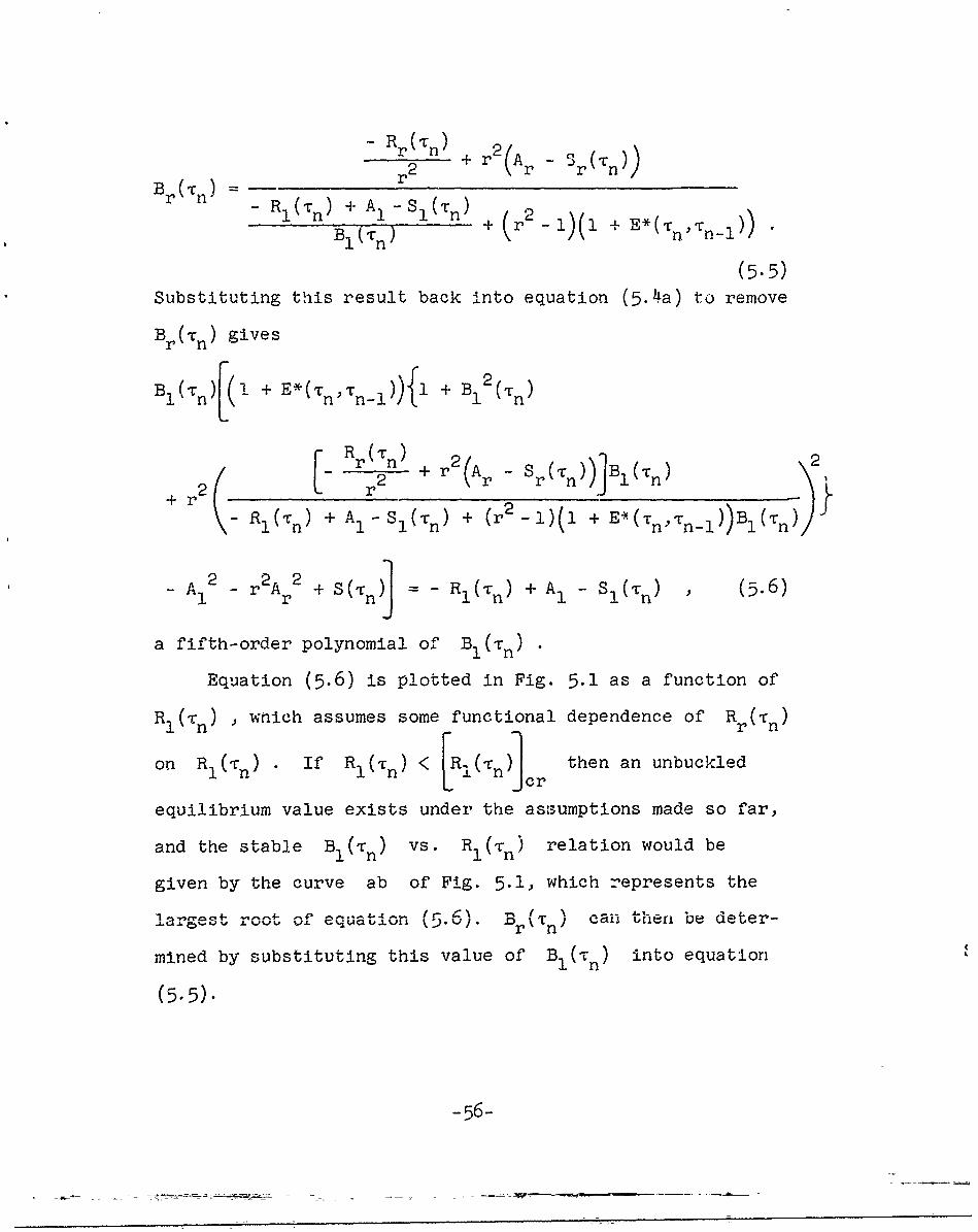
(5.5)Substituting this result back into equation (5.4a) to remove
Br(Tn) gives
BI(Tn) + E*((Tn,n-l)){l + BI 2 ( ,n )
+ r + (Ar S r ( n ]Bl(Tn)
( R1 ( n ) + A 1 -S1 (Tn) + (r2 -_)(1 + El(tni ,-_n)) Bl(n)2
-A 1 2 r 2 A 2 + S(,n)] = _ Rl(n) + A1 - S!(Tn) (5.6)
a fifth-order polynomial of B (-n )
Equation (5.6) is plotted in Fig. 5.1 as a function of
R1(n) , wnich assumes some functional dependence of Rr (Tn )
on R1 (-r) . If R)(Tn) < LRl(m) then an unbuckled
equilibrium value exists under the assumptions made so far,
and the stable BI( n ) vs. R1 (rn) relation would be
given by the curve ab of Fig. 5.1, which represents the
largest rLoot of equatLon (.6). B3f) can ten be deter-
mined by substituting this value of BI(t n) into equation
(5.5).
-56-

R1
11Bn)] n )
Fig. 5.1
-rj . .. .. .Z( , o ,i o { + 1 q (,r n
S,(-r ) ; and it. follows that Sm (T n 0 since ic was
assumed that B m(n) = 0 . Thus following an argument
similar to that used to derive equations (4.15) one gets
-57-

S('r ) = S(Tn) + E*(Tnl_ ) (2 n ) + r 2 Br pd
Sl (1 n+ ) = S! (-n) + E*(T n-i ) B1(' n )
(5.7)Sr(n + ) = S r(r ) + E*(T nTn- )B r ( 'n ) f(
Sm(-rn+) -0 m / 1,r tv
Substituting these results into equations (3.12), as was
done before, and by noting that at T = Tn+ it is desired to
apply an additional load AR and ARr . it follows that
BIn +)[I + Z k 2Bk 2 (Tn+) A 1 2 - r 2 Ar 2 + S(Tn+)1
= 1 ( I Tn ) + AR1 ) + A1 -S l(Tn+ )
an( () 2 o 2 2 S A 2 r 2a 2 3+(r r+, k nIr1 r + .(-r+)
(R(T) + r2(Ar - (5.8)
Eq,n) k22 - A 2 2 A 2 + ) = 0 E
B(r m2 + ZkBk (Tn+) - A, - r + S(- n
m/ r
It is convenient to consider as a function of 6R1
so that stability may be discussed with AR1 the lone inde-
pendent loading parameter. While this may not always be
-58-

desirable, it seems a reasonable assumption to make at tnis
point.
In the investigation of the system of equations (5.8)
there are again two possible solutions to consider. The
first will be to assume Bm (Tn +) = 0 , which allows the first
two of equations (5.8) to be rewritten so:
B ( n +) 11 + B12 (Cn+ ) +
R (n ) + Rr) +2(A r - Sr(tn+ )B(rn+)r2 r2
ri
- (Tn) + AR1) +A - S(n+) + (r 2 -l)B l(T )
-A1 2 -_ r 2A 2 + S~t) ~(- ) AR1) + A1 S1(1r 1(' +A S(rn + )
and (5.9)
_) cr(n) 2+ ARr + r2 (Ar Sr (n+))r2
-(R) 1 (T) + AR + A - Sl('rn+) 2+ (r - 1)Bl1 (-Vn+)
Equations (5.9) and (5.10) are plotted as the fuil lines onj r-.0a an c: 2b ...... 4 4 -.-,1--
_" ~ .&- &&A _ V- ,
The broken line cr in Fig. 5.2a is given by
B( n+) = ( -RTn) +__AR + A1 - S1 (-rn) (5.11)i - r2
-59-

,~ F-
,-. I 3a~Io
C) 1
04 F
L+ 4 I
i--6o-

which is found by setting the denominator of equation (5.10)
equal to zero. It can be seen from equation (5.9) that no
solutions of B1 ('rn+ ) will fall on this line except at the
singular point c , and thus all possible stable equilibrium
values fall below this line on the curve ab . Thus it is
concluded that Rl(Tn) + AR = Rs (Tn+) is the non-transi-
tional buckling load. [R!(rn)]cr as shown on Fig. 5.1 and
Rs(IL n+) on Fig. 5.2a are equal only if R1 (- n ) = [Rl(Tn)]cr
If the system is to have an unbuckled equilibrium value at
= n then it is necessary that
RI('rn) < [R 1 (n)]Cr < Rs(-rn+)
The other possible solution to the system of equations
(5.8) has one value of B( n+) / 0 , m 1, 2 . Thus the
third of equations (5.8) gives
m22 +B 2 (-r )) +rn 2B 2 (r+) AI2 _ r2A 2+ S(T+) 0m2+B2(n + + r Tn m nr n
(5.12)
With the use of equation (5.12) the first two of equations
(5-8) become
- (R, + M,) + A, -
B ( + m2 (5.13)
and(Rr (Tn) + r)+r2(A S(R( + + r2(A - S(-n+))
r 2mB r(-rn + ) = 2 _2 ' (5.14)
-61-

Substituting these two back into equation (5.12) results in
m2 Bm2 ( )n ) )A 1 t= m2 +A 2 +r A-S( )-((R l (() + 2-
2 -
+ 2r2 2 2 j r2A -1 (n + .A
r 2r 2 25r2 _m 2 •15)
If r = 2 , m > 2 and so the line given by equation
(5.13) would not intersect the cu.-ved segment ab of Fig.
5.2a, since its slope is greater than that of the line cr
Thus it can be concluded that, if r = 2, Bm(n+) / 0 is
not a possible solution and the mode of buckling will be non-
transitional (i.e. no unexcited mode will be present in the
collapse configuration).
If r > 3 , then m may take on a value less than r
and it may be possible to get a solution where Bm(-Tn+) / 0
is valid. Equations (5.13), (5.14) and (5.15) are plotted
as the dashed lines on Figs. 5.2a, 5.2b, and 5.2c respective-
ly, on the basis of r > 3 and m < r
As was the case for the sinusoidal arch with sinusoidal
load, if b' falls on the arc ab then the critical loading
is Ru(Tn+) , and by inspection of equation (5.13) it is seen
that m = 2 would give the lowest value of Ru (-r n+) . Un-
like the sinusoiaal case though, it is not convenient to
give R s(Tn +) and Ru (Tn+ ) in explicit form, since thisgniue
-62

involves the solution of a fourth order polynomial rather
than a second.
The conclusions to be drawn are:
1. If R(r n ) < Rs(Tn+) or Ru (T n+) , whichever is
smaller, then the arch is stable at T = Tn * Thus Bl('rn)
and Br(rn ) found from equations (5.4a) and (5.4b), with
Bm(-n) = 0 , are the stable equilibrium values.
2. Since Bm(T n ) = 0 as long as the arch is stable,
Sm(T n ) = 0 , and the assumption made at the beginning of the
chapter that this is so is then proven to be valid.
3. If the second mode is excitad, then any higher mode
not excited remains zero for all time, stable or unstable.
It is interesting to note the influence of an excited
nonsinusoidal mode upon the buckling load. If the second
mode is the one that is excited, then a very small amount
of asymmetry in the arch considerably lowers the critical
load. Fig. 5.3 shows a typical load deflection relation at
two different times, the dotted curve represents a sinusoidal
arch while the full lines correspond to the same arch except
that the second mode has been excited. It can be seen that
there is considerable difference in the critical load for
the two cases, and that the influence of this nonsinusoidal
excitation increases with time.
Fig. 5.4 shows the response of the same basic arch as
in Fig. 5.3 except that this case has the third mode excited
instead of the second.
-63-

R() + AR1
".[Rl (0) + lr A2 0
A2 =C
+Alcr A
{R,(0r) + 6R]c A 2 =C
Fig.- 5.3
B1.
FR (0)+L~ A =0\\ /6R1 cr3
c l 0)+AR1] crA 3 =A. C AI=
(-r) + R=01 11c
IR3 f [ + 6R, A- CA =rA>' 1Jcr
Rl( + 6R 1] A=, 3 =
R]. + AR-] A 2 A 0 3 0L~ cr
r__Fg .

I
From Figs. 5.3 and 5.4 it can be seen that the effect
of exciting the second mode on the buckling load of the arch
is much greater than exciting the third mode. It can also
be shown that exciting higher modes, either odd or even, does
not have as much effect as exciting the second mode.
As the magnitude of the nonsinusoidal excitation decreases,
the load deflection curves approach the dotted curve of the
sinusoidal arch and the cr line. Thus in the limit as the
excitation goes to zero, the critical load for the nonsinu-
soidal arch approaches the critical load for the sinusoidal
arch, as would be expected.
Figs. 5.3 and 5.4 correspond to arches that have an
initial rise-to-span ratio such that the mode of buckling is
transitional, which requires that A12 - Sl(-r ) > 5.5
where T cr is the time at which the arch buckles. If
A1 2 - Sl( +) < 5.5 , the sinusoidal arch will buckle in a
nontransitional manner. Fig. 5.5 shows the response of
such an arch with higher modes excited.
It can be seen from Fig. 5,5 that, for A2 = A3 , the
effect of the second mode being excited is again larger than
the effect due to the third mode.Comparisonof Figs. a . d 5.4 ""t 5-5 LU I
... .. ".. %ALL 5. E =Lu -hat ^or
A2 AS= 3 = constant . the influence of the nonsinusoidal mode
A1 A1
on the buckling load decreases as A decreases. For the
elastic case [11] shows plots of critical load vs. A1 for
-65-

A2 A3various ratios of 2 and 3 and these show the above
1 A1
mentioned trend very clearly.
(V.II) Several modes excited
The solution of the problem is which many modes are ex-
cited, through either the initial arch shape or the loading,
is a simple extension of the case of two modes excited.
Equations (5.1) through (5.5) remain valid except that
r now stands for any excited mode except the first mode.
Equations (5.6) can then be written as
2B!(-r) (1 + En, nl).l + B1 (,n)
nkn ('n)
+ +k 2 2(Ak -Sk(')) Bl( r2k=r RI1 ('rn) + A!1- S, (-cr) + (k- 1 ) (1 n E(n, nl ) i(
- A22 -k2Ak 2 + S(T] = - R1 (' nr) + A1 - S1 ('Ln) , (5.16)
a polynomial of B1(Tn) of order (2h + 1) , where h is the
total number of excited modes.
Equation (5.16) is plotted in Fig. 5.6. The dashed curve
in Fig. 5.6 is given by
2 2 12A2 + S(,) 1BI(-n n + E*(T )(l -+ B- A kA
n ( n-1)(1+Bl+ AI ) 1 (j
R R nTr + A 1 - S,(t1 ) ,

R,4
RI
b er
Ila
F'g.- 5. 6
R,~~n + AR1
R (t)VU r 1
Fig. 5.7
-67-

and it can be seen by comparing this to equation (5.16) that
all real solutions of equation (5.16) must fall within the
dashed curve as shown.
if Ri1 ( n) < [R1(Tn)] then an unbuckled equilibriumIfRITn <RL T cr
position exists and is represented by a point on the arc ab
B 1 n) can be calculated from equation (5.16) and the other
modes then calculated from equation (5.5). Following the
same procedure as was used when only two modes were excited
S(Tn+ ) , S1 (tn+) , S(-rn+) and Sm(Tn+) = 0 can be calcu-
lated, and equations (5.8) then give the governing system of
equations for the time T = Tn+ .
Again two possible solutions exist, the first with
Bm (Tn +) = 0 which gives
B1 ( n+ ) [l + B12 (r n + )
+7k ((k(2)+AR+ k2(A k Sk(ne B (Tn+)
- A12- Z k2Ak2 + S(-n+ = - (R1 (rn) + "1)- A1 + Sl(tn)
(5.17)
and Br(c n+) as given by equation (5.10).
The second solution with one Bm(Tn+) / 0 has
B1('n) and Br(-n+) as given by equations (5.13) and (5.14)
-68-

respectively, and B%(-,n+) is eoverned by
1 2 2 Akr&Bm (n) n m' + k S(r )
(R -n+ A~~k) +2k 1 k 2 + k -(A Sk(Tn+ ))
- > KIC(5.18)Ik=l,r k2 m2
where m l.,r
If the second mode is excited, then as before Bm(-n+)
will always remain zero, but if the second mode is not ex-
cited, Bm('n+) / 0 where m = 2 may be a possible solution.
Fig. 5.7 shows equations (5.13) and (5.17) for the case
m = 2, i.e. the second mode is not excited, Thus if bi
falls along the portion ab as shown, Ru(Tn+) is the criti-
cal loading, but if b' falls along bc or does not exist
then R (T +) is critical... n
It can be seen that the only difference in the solution
of the case where many modes are excited, as compared to the
case of two excited modes, is that the order of the poly-
nomial that determines BI() , equations (5.16) or (5.17),
is raised by two for every additional excited mode. While
this raises the possibility of having more equilibrium posi-
tions, it is noted that these additional positions are not
unbuckled stable equilibrium positions, and so in the actual
evaluation of the critical buckling load they are not a factor.
The fact that the polynomial is of higher order causes some
-69-

increase in the work required to calculate the unbuckled
equilibrium position, but this is the essential difference
between the two cases.
Figs. 5.8 and 5.9 show the ordinate B1((T) plotted
against T , the dimensionless time parameter, for a fluid
and a solid material respectively. Aside from the fundamental
difference in the two figures, caused by the fact that for
loads below a certain value the arch made of a solid material
reaches a stable equilibrium value as T - c , the response
of the two cases is qualitatively the same. It is to be
A2noted that for small values of asymmetry Al < 0.001
the ordinate is nearly identical with that of the sinusoidal
case until the critical condition is approached, at which
time it starts to diverge rather rapidly with subsequent
failure.
Figs. 5.10 and 5.11 are plots of the critical buckling
time vs. the applied load for various amount of asymmetry in
the second mode. Of particular interest is the large decrease
in the critical time for very small amounts of this asymmetry.
As pointed out previously the effect of exciting the third
or higher mode ib not as great as exciting the second mode,
but the character of the response is the same as that shown
in Figs. 5.8 to 5.11.
-70-

0H
ID 0I
N cc;
4-,
'I 0
* H -H) 0
bO X Z
cu Cu Cu

0
II 0
CO 0
0r H ~HH 0
I; a) z~-
a.) H)
'Pl, P C13
a\ c lC
UD 0 IDN
-72-

00
r4
o ~coo c 0
r*w-
0 R4 x
.. 73-

0 E-0oc
I 0
r74
0CC) 0 D

Chapter VI Long-time Solution for a Viscoelastic Solid
Material
If the arch is made of a viscoelastic solid material,
and the loading approaches a constant as T becomes large,
then there is a possibility of the deflection reaching some
final stable value as T - c .
Letting TP denote T as it becomes very large, equa-
tions (3.21) can be written as
Bm(,"F)
+ Z k F-Ak+) Z k 2 ( 2k=l (Bk or) k + 0 k=l k
00= 2 + m m- fE (- Am d(6.1)
m om
m = 1,2,3, ....
In the evaluation of the integrals it is to be noted that
Bm( ) is essentially constant and equal to Bm(-F) for
e-+ F * For e small B() varies but E ( F - e) -- 0
since (TF-e) becomes very large. Therefore in the rangeof e where Ei(TF-) is different from zero B (e) is
nearly constant and so can be taken out from under the in-
tegral sign. Thus to a good approximation
F El(-0 ( ( ) - Am)d = EF -m
~E 0(Bm(TF)0+ 0 A
where EF = (0) . (6.2)
-75-

Similarly,
P Et-F0Sz k2 (B ) - Ak 2)d+ E0 k=l
E Z k2(B 2 () - A 2 ) . (6.3)
E0 k=l .
Substituting equations (6.2) and (6.3) into equations
(6.1) gives
2m Bo 2, Ak2 C\L E R m (TF) m2A (
Bm(F){2 + ( kiTF) -k o mF m-I- I-+m , (6.4)k=l1 Y F m
m = 1,2, ... .
Equations (6.4) are identical with the equations of an
elastic arch of modulus EF under the same loading; but
in the viscoelastic case they can only be used to determine
the unbuckled equilibrium position denoted by the ordinates
Bm(TF) , since in their derivation it was assumed the arch
was stable under the loading Rm(F) and had reached a
final configuration.
To check the stability at T = T F ' subject the arch
to an additional load at T = TF+ in the same manner as
was done previously in Chapters IV and V. Bm(TF) can be
calculated frm. equat-ions (6.), considering any unexcited
modes to remain zero. If an unbuckled solution of equations
(6.4) does not exist, this indicates the arch has buckled
at some previous finite time. On the assumption that
Bm(-F) exists, the integrals S(TF+ ) and Sm('rF) (see
-76-

equations (4.15) or (5.7) ) can be evaluated, thus
Et(r F- E) W2 2
S ()k=+) ( E )
Sm(rF+ ) E ( m(TF) - Am)
The governing equations for Bm (r F+) then become, from
equations (3.30)
Bm (F+){m2 + z k2(Bk2 (TF+)- Ak2 ) S ( Fk=1
- R ~R(rF) + + .2 (A.-sl(LF) (6.6)
m = 1,2,3,....
The solution for this set of equations and the method
of determining stability are given in Chapter IV or Chapter
V, depending on the number of excited modes. If it is found
that (AR.) < 0 , this indicates that the arch has buckled
at some previous finite time.
It is to be noted that the critical load found from
equations (6.6) differs from the critical load of a purely
elastic arch of modulus E0 that has the same deflected
shape as the long-time solution of the viscoelastic arch
under the same loading Rm(tF) . This is due to the fact
-77-

that, although the two arches support the same load with the
same deflected shape, the axial thrust and moment distribu-
tion are not the same in both cases. This arises because the
moment is directly proportional to the deflection while the
thrust is proportional to the square of the displacement.
In [11] it was shown that, for a uniform load on a sinu-
soidal arch, the effect of the higher modes, i.e. 3, 5, 7, ... ,
was to reduce the critical load by no more than .5% of the
critical sinusoidal load. That this is not valid for the
viscoelastic case can be expected from the results of Chapter
V, where it is seen that near the critical buckling time the
displacement of the non-sinusoidal arch differed considerably
from the displacement of the sinusoidal arch (see Fig. 5.9).
The reason for this can be seen from an examination of equa-
tions (5.17) and (5.18). In each of these expressions there
is a series of the form
(*(Rk ("n + M k + k 2(Ak Sk (-r)) 2
Z k_2 k 2 2 (6.7)k=r k m
where r includes any excited mode other than the first.
in order to illustrate the effect of the viscoelastic materi-
al, consider the case of a uniform load on a sinusoidal arch
which has RRr(t) r Y r = 3, 5, 7,
0 , r = 2, 4, 6, .9
and A =0 r / 1
r-78-

ISubstituting these into the series (6.7) results in
k 2 2 ( 6 .)
k=3,5,7... (k2 _ m 2 )2 k n
In the elastic case S k(T) 0 and the series (6.8) is re-
dluced to
(RI( n ) + R) 2 (6.9)
k=-5,7.. • m
w:hIch is a very rapidly converging series. For m 2
T/ 2 4) 4.977 x 10- 4
k= 5,7 k.7 (k
and so the effect of the higher modes oi, the elastic critical
load is seen to be negligible. However, for the viscoelastic
case S r(-Cn +) / 0 , and so the second term of the series (6.8)
leads to an expression of the form
k 57 (2k 6 S 2(Th +) (6.10)k=3,5,7 \k 2 _ m2) k
which could be divergent, depending on the values of S (t +)r n
While it is not possible to express explicitly S (- + ) -,s
a function of r It is ae.- that in the long-time solitlon
Sr(tn+) varies directly as Br(,rF) (see equation (6.5)),
and that
I
-79-

F R,(-cF)
E° r 3 (6.11)
r(F = Rl(cF) + A1 2BI('tF) + (r 2 - )
r = 3, 5, 7 ..
Equations (6.11) are derived from equations (6.4) for a
uniform load on a sinusoidal arch. Thus it is seen that
for large r , Br(- F ) varies as - and so the conver-r5
gence of the series (6.10) is assured. The fact remains
however, that the series (6.8) may not be negligible since
some of the lower terms may have appreciable magnitude, and
cannot be neglected in the calculations. Added to this is
I the fact that the terms S(-rF+ ) and Sr(TF+) appear in
other ways in equations (5.17) and (5.18) and must be ac-
counted for.
Figs. 6.1 to 6.4 show the effect of EF and Rl(rF)
on the buckling load of an arch with initial rise A, = 4
Compared to Fig. 6.1, which is the purely sinusoidal case,
he otl her f.g.... show a very rapid decrease in the critical
load as R!(- F ) increases. This can be attributed to the
fact that the amplitude of the higher modes in the unbuckled
configuration increases very rapidly as the load approaches
the critical load (see Fig. 5.2).
-80-

1u 7
+F
122
R 1(-rF)
Fig. 6.1 Three Parameter Solid Materisl ialLa
Sinusoidal Arch A~ 1 4 , SinusoidlLa
'p'
13-
2 6 001
Fig. 6.2 Three Parameter Solid Material
Sin-osoidal Areri A ~ Un4liformn Load

EF = *
12 Ev .
+ F -
68 10 r
R1 (F
Fig. 6.3Three Paramneter Solid MaterialFi. .3Norisinusoidal Arch- A =
Sinusoidal Load1
14 EF
EF =.7
R(F) 0. 01
+
11 10 F
1'71
Fg.6A4 Three Parameter Solid Material
Sinlusoidc-l Arch A,. 4
Norisifusoidal Load ±
-82-

Chapter VII General Features of the Numerical Solution
The numerical integration and solution of the roots of
the algebraic equations were performed on the B-5000 digital
computer at Stanford University.
In the numerical integration of integrals of the type
E( ) (7.1)o+ 0
it is advantageous to use a variable time step if the form
of the functions E(T) and f(T) are of the requisite type.
E'(-) varies quite rapidly for T small but as T becomes
large EQ(T) approaches zero. In this problem, where f(-r)
represents functions of the type (Bm(-r) - Am ) , it is
possible to draw several conclusions regarding the behavior
of f(-) if the loading functions Rm (T) are sufficiently
smooth. For T small f(T) will vary quite rapidly, re-
gardless of the type of viscoelastic material, but for T
large the material property makes a considerable difference.
For a fluid material it is expected that f(T) would con-
tinue to vary quite rapidly until failure takes place, es-
pecially if the time at failure is quite small. On the other
hn% If thel mats1 a vscoela solid the variation
at large times will be quite small, except near the critical
time.
In order to take advantage of these facts and reduce
the computing time, a logarithmic time step increment was
-83-
- - ---. ~~-=- ~-.=

used (see [151) until the critical time was found, at which
time the program reverted back to the last known stable time
and a smaller time step introduced. In this manner small time
steps were used for -r small and r near the critical time,
while larger steps were used where E'(T) and f(-) varied
more slowly.
Among the roots B1((T) , only the largest root of Bl( )
is required in the analysis and so a simple iterative type
solution was used. Convergence was very rapid for solutions
near the point a of Fig. 4.1 but became slower as the equi-
librium value approached b , at which point the program would
not converge.
If the progrmm would not converge a check was made to in-
sure that no unbuckled equilibrium solutions existed, as this
constitutes one possible mode of failure. The second possible
type of failure, that of an unexcited mode becoming non-zero,
is easily checked by calculating B (T) on the basis of
B(T) / 0 (see for example equation (4.9) ), then if the
B1 (T) found in this manner is greater than the B1 (T) found
from the iterative solution, the arch is unstable.
The time step increments and the allowable tolerance in
the iterative solution were adjusted so that the solution for
B1 (T) was accurate to at least four significant digits in
all the test cases considered. The maximum computer time
needed was less than one minute for any one problem including
a case where ten modes were excited and the maximum time taken

to be 1000.
In Chapter VI there are no time integrations to be per-
formed, but in order to find the critical load for equations
(6.6) it was necessary to use a double iterative procedure.
One iterative procedure is required to determine the un-
buckled equilibrium position, and a second is then required
to find the critical buckling load. Thus, although the
programming is quite simple, considerable machine time is
required in its execution.
-85-

t
* REFERENCES
1. Timoshenko, S. P. and Gere, J. M., THEORY OF ELASTICSTABILITY, 2nd Edition, McGraw-Hill.
2. Kempner, J., Viscoelastic Buckling", HANDBOOK OF ENGI-NEERING MECHANICS, ed. W. FlUgge, McGraw-Hill, 1962.
3. Kempner, J. and Hoff, N_ J., "Behavior of a Linear Visco-elastic Column", Appendix II to Hoff, N. J., Struc-tural Problems of Future Aircraft, Proceedings of theThird Anglo-American Aeronautical Conference. theRoyal Aeronautical Society, London, England, 1952,p. 110.
4. Kempner, J. and Pohle, F. V., "On the Nonexistence of aFinite Critical Time for Linear Viscoelastic Columns'Journal of the Aeronautical Sciences, Vol. 20, No. 8,P. 572, August 1953.
5. Hilton, H. H., "Creep Colla~se of Viscoelastic Columnswith Initial CurvaL Ares , Journal of the Aeronauti-cal Sciences, Vol. 19, No. 12, p. 844, De3ember 1952.
tit
6. Lin, T. H., t, resses in Columns with Time-DependentElasticity', Proceedings of the 1st Midwestern Con-ference on Solid Mechanics, 1953.
7. Lin, T. H., "Creep Stresses and Deflections of ColumnsJournal of Applied Mechanics, Vol. 23, No. 2, p. 214,June 1956.
8. Hilton, H. H., "On the Nonexistence of Finite CriticalTimes for Generalized Linear Viscoelastic Columnswith Arbitrary Initial Curvatures", Journal of theAerospace Sciences, Vol. 28, No. 8, August 1961.
9. Goodier, J. N. and Ramsey, H., "Problems of Related Elas-tic and Viscoelastic Buckling in One and Two Dimen-sions", Stanford University Engineering MechanicsTechnical Report No. 133, July 1962.
10. Pian, T. H. H., "Creep Buckling of Curved Beams UnderLateral Loading", Proceedings, Third U. S. NationalCongress of Applied Mechanics (Brown University)(ASME) 1958.
11. Fung, Y. C. and Kaplan, A., "Buckling of Low Arches orCurved Beams of Small Curvature", NACA Technical Note2840, November lqcji2.

12. Bland! D. R., THE THEORY OF LINEAR VISCOELASTICITY,Pergamon, 1950.
13. Lee, E. H., "Viscoelastic Stress Analysis", First Sym-posium on Naval Structural Mechanics, ed. J. N.Goodier and N. J. Hoff, Pergamon, 1950.
14. Lee, E. H. and Rogers, T. G., "Solution of ViscoelasticStress Analysis Problems Using Measured Creep orRelaxation Functions", Journal of Applied Mechanics,Vol. 3 0, p. 127, July 1963.
15. Lee, E. H. and Rogers, T. G., "On the Finite Deflectionof a Viscoelastic Cantilever", Proceedings, FourthU. S. National Congress of Applied Mechanics (Berke-ley) (ASME) 1962.
16. Hoff, N. J., IA Survey of the Theories of Creep Buck-ling , Stanford University Aeronautical EngineeringReport No. 80, June 1958. Also Proceedings, ThirdU. S. National Congress of Applied Mechanics (BrownUniversity) (ASME) pp. 29-49, 195b.
17. Gjelsvik, A. and Bodner, S. R., "An Investigation ofthe Energy Criterion in Snap Buckling Problems withApplication to Clamped Arches", Brown UniversityEngineering Technical Report No. 28, February 1962.Also "The Energy Criterion and Snap Buckling ofArches", Proceedings of the A. S. C. E., Vol. 88,No. EM5, October 1962.
-8~-
Recommended


![Engineering Mechanics - DrChawin.com Engineering Mechanics I [Statics] Lecture 1 Page 1 of 12 Lecture 1: Introduction to Engineering Mechanics Engineering mechanics is the …](https://img.pdfslide.us/doc/110x75/5aa4d6047f8b9ab4788c63da/engineering-mechanics-engineering-mechanics-i-statics-lecture-1-page-1-of-12.jpg)