DISTRIBUTED LAGS
by
Christopher A. Sims
Discussion Paper No. 28, March 1973
Center for Economic Research
Department of Economics
University of Minnesota
Minneapolis, Minnesota 55455
DISTRIBUTED LAGS
by
Christopher A. Sims
A time series regression model arising in econometric
research ought in nearly every case to be regarded as a dis-
tributed lag model until proven otherwise. From this point
of view, "distributed lag" methodology extends over a large
fraction of econometric methodology, too large a fraction to
fit into a relatively short survey paper. So much has gone
on in the study of econometric time series regression methods
since the survey by Griliches (1967) which I will take as a
base, that the recent publication of a broad book in the area
by Dhrymes (1971) and of a survey of some aspects of the area
by Nerlove (1971) reduce the ground this survey should cover
by no more than enough to make it manageable.
Let us introduce some notation and definitions. A dis-
tributed lag model in discrete time is a regression equation
of the form
1 ) Y ( t) = 1 CX)b ( s ) x ( t - s) + u ( t ) . s=-·o
where y(t) and x(t) are in principle observable, u(t) is an
unobservable error, and b is an unknown function, called the
"lag distribution". Values of b(t) for positive t apply to
past, or lagged values of x, and are referred to as coefficients
for "positive lags". Similarly values of b(t) for negative t
are coefficients for negative lags, i.e. for fUture values of
x. A convenient notation is to write
2) b*x(t) = L ~b(s)x(t-s) s=-·o
-2-
Here the two functions on the integers, b and x, are mapped
into the new function on the integers, b*x, by the convolution
operator n*n. Thus equation (1) becomes
3) y = x*b + u.
Convolution behaves formally much like multiplication. Certain
restricted classes of functions have well-defined inverses
under convolution. The restrictions which imply the existence
of an inverse are probab~ very often met by lag distributions b,
though very seldom by independent variables x.
The Fourier transform b of a f~nction on the integers b
is defined by
-4) b (w) = I ""b(s)exp(-ims ) • s=-·"
Its usefulness in the theory of distributed lag models arises
- -from the fact that (b*c) = b c, i.e. that the Fourier transform
converts convolution into ordinary multiplication.
Thinking of lag distributions as polynomials in the "lag
operator" is another way of achieving the same notational and
heuristic conveniences available from the Fourier transform and
the convolution operator. Readers not familiar with convolutions
but who have read, say, Griliches' (1967) exposition of formal
manipulation of lag operators, should be able to interpret
the notation of the present paper easily by thinking of "*"
as multiplication of polynomials in the lag operator. The main
advantage of the convolution and Fourier transform apparatus is
that it generalizes more naturally than the lag operator to
continuous time models.
-3-
Though (1) is the basic model of this paper, most applica
tions i.;ill involve extensions of (1) to include several variables
on the right-hand side of the equation. This creates no essential
complication. Also, the doubly infinite range of summation
in (1) is of course not meant to exclude models in "'hich 'de
know a priori that b(s) = 0 for all s < 0, or even purely con
temporaneous regressions, where b(s) = 0 for all s ~ O.
Extensions of the theory to cover applications where several
equations of the form (l) are treated as a system do involve
fundamentally new elements, and such extensions are considered
only briefly in Section 7 of this paper.
Section 1 below consists of remarks on the subject which
is the main concern of Nerlove's survey, the relation of dis
tributed lag regressions to economic theory. Section 2 consists
of remarks on the theory of estimation for regression equations
containing autoregressive terms, a subject treated thoroughly
by Dhrymes. Section 3 takes up frequency-domain (or spectral)
estimation methods, attempting especially to assess their
relation to other estimation methods and offering some new
results in that direction. Section 4 considers two types of
"nuisance" specification error peculiar to distributed lag
regression: neglect of seasonal noise and the pretense that
time is discrete. Section 5 describes recent advances in the
treatment of collinearity problems in distributed lag models
by introduction of prior beliefs in the "smoothness" of' the lag
distributions. Section 6 is concerned with statistical tests
-4-
for the presence of two types of specification error not peculiar
to time series regression, but for which the appropriate form
of the test is peculiar to time series regression: These are
failure of the assumption of spherical errors (serial correlation)
and failure of the exogeneity assumption (feedback). Section 7
touches very briefly on the subject of systems of time series
regressions. And Section 8 contains concluding comments.
1. Dynamic Optimization Theories as a Basis for Time Series Models
Griliches (1967) speculated pessimistically in his survey
that most data might contain little information on the detailed
questions about dynamics which we ask of them; he concluded
that "progress in this area is likely to be slow until we have
a much better theoretical base for imposing a time-lag structure
on the data". Since 1967 there has certainly been growth in
dynamic economic theory and in efforts to apply it to distributed
lag models, but a reading of Nerlove's (1971) survey, which
concentrates on these issues, suggests that the role of better
economic theory here has once again been for the most part not
to provide us with solutions, but to help us better understand
the limits of our ignorance. Early work deriving distributed
lag models from optimizing theories, like that underlying
Jorgenson's (1963, e.g.) extensive work on investment which
Griliches cited, faiJed to follow through completely on the
program Gf' using an "optimizing" theory. The economic agents
under study were assumed to optimize only within the bounds
of a "static expectations" or "adaptive expectations" assumption,
-5-
that is, an assumption implying that they did not optimize their
techniques of forecasting. Though Muth's seminal article on
rationaJ expectations appeared in 1961, the difficult program
of bringing the rational expectations hypothesis useful1y into
the optimizing theories used to generate applied distributed
lag models is still only beginning. This problem of the proper
handling of expectations now appears as central to any attempt
to build a usable bridge between theoretical and empirical dynamic
economics.
The first step, emphasized by both Nerlove in his survey
and Tinsley (1971), is to formulate the optimization problem
initially without trying to eliminate future values of variables
from the model. Direct solution ,vill then in general show
decisions in the current period dependent on future values of
variables. Getting even to this point in a realistic economic
model may be a substantial task, as Tinsley's paper makes clear,
but Nelilove emphasizes that what may be the most important and
most difficult task still remains. To get a theory with content
concerning the dependence of decisions on the past, we require
an explicit formulation of the stochastic nature of information
flow to the decision-maker. Nerlove suggests in his survey the
hypothesis that knowledge about future values of a variable is
based on current and past values of the variable and that
decision-makers use this information "rationally" in ;;'uth' s
sense.
-6-
Nerlove's contribution in his survey is particularly
weighted toward suggestions for approximations and simplifica
tions which may allow us to construct models in which: optimiza
tion of forecasts is an integral part of the structurej the
structure is mathematically completej the model is computationally
and analytically manageablej and the model is realistic enough
to be useful. This is an ambitious goal, as yet no more than
partially realized in any application, as we will discuss below.
But even where Nerlove' s goal cannot be ful1y achieved, the
rational expectations hypothesis has proved fruitful.
The most familiar example of an economic theory incorporating
rational expectations is Friedman's (1957) permanent income
theory of consumption. Though it appeared before Huth gave
the rational expectations hypothesis a name, Friedman's theory
illustrates the insights to be gained from the hypothesis,
some of the limitations of such insights, and the potential
gains from more formal use of the hypothesis along the lines
Nerlove has indicated.
Friedman observes that, for a rational consumer under
perfect certainty, current consumption depends on the entire
future time path of income. Since an individual's current
income is unlikely by itself to carryall the information
about future income available in the history of' his income,
it follows that his consumption is likely to depend on a dis
tributed lag in income. Friedman does not investigate the
mathematical relations between the serial correlation properties
-7-
of the income time series and the nature of the income-consump
tion regression (and we will shortly take up that issue), but
clearly Friedman's theory implies that the nature of the dis
tributed lag relation between consumption and income should
depend on the nature of the income time series. If the serial
correlation properties of the income time series should change,
or if income changes due to an identifiable event not related
to future income in the same way as usual fluctuations in income,
the response of consumption m8¥ differ from what is implied
by distributed lag regressions fitted to historical data.
Changes in income due to changes in tax rates in particular may
not produce the historical pattern of response in consumption:
The response may be more rapid if tax rates have always changed
very infrequently; the response may be weaker if a flexible
system of countercyclical changes in tax rates has been announced
and introduced.
This negative result of the rational expectations hypothesis,
that lag distributions arising from expectation-formation must
be expected to change with changes in the serial correlation
properties of variables being forecast and to be different
for changes in the same variable arising from identifiably
different sources, reappears in every application. Since
consideration of the optimizing behavior underlying econometric
distributed 1 ag relations nearlY ahmys shows an expectatLmaJ
element to be present, and since the rational expectations
hypothesis surely captures at least part of the truth about
the way people form expectations, we reach certain general
-8-
c:)nc'usions about distributed lag methodoJ·::Jgy. One is that
static theory is not a reliable guide to selection of variables.
That static theory implies total income from non-human and
human wealth is all that enters the consumption decision does
not imply that both types of income affect consumption with the
same lag distribution. That static theory implies the interest
rate and tax rates affect the investment decision only th:rough
their effect on the cost ot' capital does not imply that separate
dynamic influences of the two variables can be replaced by a
single lag distribution on the cost of capital. These are
both analogues of the point that tax changes may effect consump
tion differently according to how "permanent ll they are seen to be.
Another general conclusion for distributed lag methodology
is that either our habit of treating the regression of endogenous
on exogenous variables as a unique function of the "structure"
of the model must change, or we must accept the idea that ,,,hat
is called the structure in textbook treatments of simultaneous
equation models can change under policy changes which affect
only the time path of exogenous variables.
An exploration of the mathematics of optimal forecasting
shows that, ,.,here expectationa 1 elements enter the formation
of a lag distribution, some widely accepted notions about
interpreting estimated lag distributions are questionable.
The sum of coefficients in an estimated lag distribution is
commonly interpreted as a "long run effect", for example.
Theories with implications about long run effects are therefore
-9-
tested by statistical tests on the sums of coefficients in
estimated distributed lag regressions. However, long run
effects could only appear if exogenous variables were permanently
moved to new levels. Such an alteration in the nature of the
exoger.ous variables cannot, as we have noted above, be expected
to leave distributed lag regressions unchanged. Hence lag
distributions estimated from historical samples cannot be held
fixed in performing the mental experiment of making long-run
changes in exogenous variables. To make this point concrete,
Lucas (1970) developed an explicit, though simple, model in
which a permanent shift in the rate of inflation has no long
run effect on the level of employment, yet distributed lag
regressions relating unemployment to the rate of inflation will
not in general have coefficients summing to one. Lucas cites
several examples of previous research in which sums of coeffi-
cients in lag distributions had been given the common, inappro-
priate interpretation in relation to just this issue.
Just as coefficients on past values of a variable in the
optimal forecasting expression do not ordinarily sum to one,
they also are not ordinarily "smooth". In fact for time series
with stable patterns of serial correlation (covariance-stationary
stochastic processes, to be precise) a rule of thumb would be
that the smoother the time series, the more oscillatory will be
the weights in the optimal scheme for forecasting the series
from its own past.l! An example of estimated optimal forecasting
weights for two-step ahead forecasts of quarterly GNP taken
-10-
from postwar deseasonalized U.S. data, is
5) ~ V y(t) = 1.74y(t-2) - .81y(t-3) - .38y(t-4) + .28y(t-5) .
To the extent that forecasts are the basis of lag distributions
in an econometric model, we clearly do not have a priori
"knowledge" that the lag distributions are smooth except by
appeal to some special feature of the model. This point is
important for Section 6 below.
Despite its success in helping us interpret, or avoid mis-
interpreting, distributed lag estimates, Nerlove's complete
program as described above has not yet been often implemented.
Nerlove (1971) and Lucas (1970) both propose the possibility
that: 1) variables whose future values affect behavior be
assumed to be realizations of stationary stochastic processes;
2) economic agents be assumed to understand the covariance
structure of these processes well enough to form least-squares
linear forecasts; and 3) the behavior of agents be described
as substitution of linear least-squares forecasts of future
values in place of the future values which enter a solution
under an assumption of perfect foresight. These assumptions
are restrictive, possibly in crucially inaccurate ways, as both
Nerlove and Lucas understand. Nonetheless, even if the assump-
tions are granted, what is gained is a useful set of cross-
equation restrictions, rather than, in Griliches' words, a
"time-lag structure" ready for "imposition" on the data.
Consider the following schematic example. Firms in a
competitive industry choose a variable I(t) we shall call
"investment" on the basis of a variable p{t) we shall call
-11-
"price". Price is exogenous to the industry, and because of
adjustment costs or frictional factors of some sort ret) adjusts
to pet) with a distributed lag. We could estimate the relation
via the regression equation
6) ret) = b*P(t) + u(t) .
We may be prepared to set bet) = ° for t < 0, on the
grounds that firms know no more about future pIS than they
can project from past PIS. But beyond that the appeal to
"friction" and "adjustment costs" gives us very little"to go
on in finding a form for the b(s) function. It is in this
sort of situation that Griliches felt that we might be asking
too much of time series data in trying to get precise estimates
of b, and that Sims (l972b) showed that hypotheses about, e.g.,
the mean lag or sum of coefficients might be untestable.
Suppose now that we introduce an explicit dynamic optimiza
tion, solving to obtain the equation
7) ret) = c*p(t) ,
where c(s) = ° for t > o.~ If pet) is a covariance-stationary
stochastic process with no exactly predictable components, then
we can expect it to have an autoregressive representation of
the form
8) q*p(t) = v(t)
where q(s) = ° for s < 0, vet) is serially uncorrelated and
uncorrelated with pes) for s < t. It is a standard result21
that the least-squares linear forecast of p(t+s) on the basis
at' p(u), U=-ao, ••• , t, is q-l*~t(t+s) .... 'here ~t(s) is a series
-12-
defined by ~t(S) = 0, s > t, ~t(S) = q*p(s), s $ t. Thus (7),
(8), and the assumption that firms replace unknown future pt s
by linear least-squares forecasts in their decision-making lead
us to
9) I(t) = c*q-l*li (t) .W t
Equation (9) is, as can be easily verified, a linear dis-
tributed lag relation of I to current and Tlast P. An error
term could be added to (9) on, say, the assumption that variaoles
other than past prices influence expectations but that these
other variables are unrelated to past prices.
Equation (9) bas a more complicated structure than the
ad hoc equation (6), and we now have a relation between parameters
in (9) and the parameters in (8) which is in principle testable.
But in place of the single equation (6) with a single essentially
unrestricted lag distribution b, we now have two equations,
(8) and (9), containing two essentially unrestricted lag dis-
tributions. The form of c depends on the precise nature of
frictional elements in the firm's objective function. Though
our knowledge in this area is extremely limited now, there is
a prospect of increasing our knowledge so as to find a basis
for interpreting estimates of lag distributions like c. But
economic theory does not even in principle have much to say
about the form of q. The length, mean lag, and sum of coefficients
in q all enter directly into the corresponding functions of the
lag distribution in (9) (i.e., b in (6». Rather than giving
us a basis in economic theory for imposing restrictions on b of
-13-
the kind which might allo\ol' us to avoid the difficulties of
estimation in infinite-dimensional parameter spaces as brought
out by Sims (1971b, c, 1972b), Nerlove's suggested implementa-
tion of a rational expectations hypothesis has led us to a
formulation showing that economic theory is probably incapable
of generating such restrictions.
That it fails to generate such powerful restrictions is
by no means a criticism of Nerlove's proposal in itself. Use
of' (8) and (9) together allows us to separate those parts of
the dynamics of the system related to the production technology
from those parts related to the structure of the flow of informa
tion. Where it is possible,1I this is an elementary and important
step toward making sense of the results of estimating the dis-
tributed lag regression (6).
Severe practical difficulties still stand in the way of
implementation of Nerlove's ideas, and Nerlove's own explanation
of the difficulties will not be repeated here. One obstacle
Nerlove did not emphasize, perhaps because it is so obvious,
is the unrealistic nature of the assumption that a variable's
own past values are the basis for rational expectation-formation.
The reason for mentioning this point here is that Shiller (1972)
has made a suggestion which may contribute toward bypassing
this particular obstacle. Suppose variables in addition to
past prices are in fact used by firms to forecast P in (7).
Then (9) contains an error term and must be rewritten
10) -1 ,. t
ret) = c*q *ut(t) + c*E (t), where
-14-
t ) A -1 A ( ) 11) E (s = P(s,t) - q *ut s ,
A
p(s,t) being the actual forecast by the firm of pes) based
on information available up to time t. Shiller points out
that the term C*Et(t) is uncorre1ated with all current and
past values of P if expectations are linear least squares
predictions from past data. Hence (10) can be estimated con-
sistently by least squares under standard assumptions. If
we have some independent way of identifying c, we can still
compare estimates of q from (8) and (10) as a test of the
rationality of expectations.
Of course if (8) is not assumed to capture the complete
expectations-formation mechanism, estimates of q from either
(8) or (10) cannot be used to generate "expected P" series.
Also if P is a vector, then q in (8) must be allowed to be a
general matrix fUnction. That is, Shiller's idea requires
that all variables on the right-hand side of the distributed-lag
regression (10) be used on the right-hand side of each of the
regression equations implied by (8), rather than each variable
being fitted to past values of itself alone.§! Finally, the
right-hand side variables in (10) are not strictly exogenous
in (10), so the usual methods of obtaining efficient estimates
in time series regressions (generalized least squares and variants
thereon) cannot be applied. If the c*Et term were the only
source of random disturbance in (10), then it would be possible
to specify serial correlation of the error term and the cross-
correlations of the errors with the independent variables as
-15-
determinate functions of c and q, making maximum likelihood
estimation possible. other sources of random disturbance are
probably important in investment function applications, but
possibly in some applications (for example, in Shiller's own
application to term structure equations) the c*Et term does
dominate the disturbance.
When there is a random disturbance added to (10) aft~r the
c*Et term, estimation by least squares remains consistent only
if the additional disturbance is uncorrelaten with current and
past P. Since the additional disturbance is not generated by
forecast errors, it is reasonable to require that P be strictly
exogenous with respect to the (unobservable) additional com
ponent of the disturbance. This implies that the cross-correla
tion function of P with the compound disturbance is the same
function of q and c as is the cross-correlation function of
c*Et with P, which is a testable implication. Applications of
the Shiller idea to rational expectation models ought to include
this test as a check on the model's internal consistency.
Let me mention in conclusion two obvious reasons for not
expecting universally good results from a rational expectations
hypothesis. Not everyone is rational, especially in the short
run. In some applications (e.g., the theory of efficient
markets) this fact may not matter much if some people with large
resources are rational. But in explaining wage and employment
behavior this fact could be crucial. Also, economic mechanisms
are at best approximately stationary over certain periods. In
-16-
optimizing over long time horizons it may not be rational to
rely on stationary autoregressive models for forecasting.
2. Regressions with Lagged Dependent Variables
Suppose we are dealing with the distributed lag model
l2) yet) = b*x(t) + u(t) ,
-1 and for some reason we think we can write b = c *q for some c
and q. Then clearly we can convolute (l2) with c to obtain
13) c*y(t) = q*x(t) + c*u(t).
If c and q are both short (that is, zero except for a few values
of t), then we may have gained something by moving from the
formulation (l2) to the formulation (13). The former will in
general involve an infinite lag distribution b, whi:e the
latter involves only finitely many coefficients.
If we know that c*u is serially uncorrelated, we can
rewrite (13) as
13' ) yet) = m L - c(s)y{t-s) +
n L q(s)x{t-s) + vet) ,
s=l 8=0
where vet) = c*u(t), and obtain asymptotically efficient estimates
by applying 018 to (13'). But there is seldom any good reason
to believe a priori that c*u will be serially uncorrelated, and
if it is serially correlated, least-squares estimates will not
be consistent. Once we admit that c*u is likely to show serial
correlation, estimation is not simple, regardless of which of
the equivalent equations (13) and (12) we choose as a starting
point.
Thus when (l2) is the natural economic formulation of the
relation to be estimated, transforming to (13) should not be
-17-
r~garded as a technique for simplifying the estimation problem.
Nonetheless there are applications where (13) itself is a
natural economic formulation,21 so that study of estimation
methods for (13) is of inherent interest.
This subject is a large one, in which there have been
important advances recent~. Luckily Dhrymes (1971) makes this
subject a central focus of his recent book, so that the reader
can be referred there for a thorough discussion. Two ideas
from Dhrymes' book are worth particular emphasis. First, in
this type of model maximum likelihood procedures are in general
asymptotical~ more efficient than the various consistent
"two-step" procedures which have been proposed.lQ/ Two-step
procedures use some consistent proceddre for estimating the
pattern of serial correlation in c*u as step one. Then in step
two they use the estimated pattern as if it were the true
pattern in transforming (13) to eliminate the effects of serial
correlation in an ordinary least squares regression or in
estimating (13) by generalized least squares regression. If
all the right-hand side variables in (13) were strictly exogenous,
there would be in most cases a large class of two-step procedures
asymptotical~ as efficient as maximum likelihood. That this
does not hold when (13) contains lagged endogenous variables
is an important feature of the model which is on~ recent~
coming to be widely understood. When the pattern of serial
correlation in u 1s not related to the form of b, maximum
likelihood applied to (13) or equivalentLy to (12) with the
-18-
parameterization b -1 = c *q is asymptotically equivalent to a
two-step procedure applied to (12). The first step obtains a
consistent estimate of the serial correlation pattern in u.
The second step uses this estimate as if it were exact in a
generalized least squares (non-linear) estimate of (12).
With this general result on the inefficiency of two-step
estimators applied to (13) before us, it seems apparent that
when (13) with finite c and q is only a convenient approximation,
no more firmly grounded in the economics of the model than (12)
with finite b, there is nothing to be gained by using (13)
instead of (12). My personal impression is that finite parameteri-
zations of (13) are somewhat more likely than finite parameteriza-
tions of (12) to give reasonable-looking results even when the
model is badly specified. Needless to say this is if anything
a disadvantage, not an advantage, of using (13).
A second important idea in the Dhrymes book concerns
use of frequency-domain methods in estimation of models like
(13). In his Chapter 10 Dhrymes shows (following the lead
of Hannan (1965» that frequency-domain techniques allow
asymptotically efficient estimates of (13) under extremely
general assumptions about u--much more general, for example,
than the assumption that u is a finite autoregression or
mixed moving-average-autoregressive process. This point,
that very general patterns of serial correlation in u can be taken
into account without any loss of asymptotic efficiency relative
to narrower assumptions about serial correlation, suggests that
-19-
the common assumption in applied work that u or c*u is a first
order autoregression is a bad one. If the assumption is very
far wrong estimates may be badly biased, whereas if it is
right there is little gain in efficiency over a more general
assumption. A recent paper by Schmidt (1971) provides Monte
Carlo evidence that comparing the assumption of first-order
serial correlation in u(t) with the assumption of second-order
serial correlation in u(t) in the simple model with q(t) = 0,
t # 0, c(t) = 0, t < ° or t > 1, the narrower assumption, even
when true, results in essentially no gain in efficiency over
the broader assumption in sample sizes as small as 20. Engle
(1972) shows that use of an assumption that serial correlation
is first-order when in fact it is higher-order may actually
decrease efficiency below that of OLS. Furthermore, the
possibility of allowing for extremely general patterns of
serial correlation ought not to be identified with frequency
domain methods solely. Frequency-domain methods make such
general assumptions very natural, but once we understand how
the increased generality of the frequency-domain methods is
achieved, the same generality is available in the time domain.
Even the computational problems in carrying through the time
domain analogues of these procedures, given strong emphasis by
Dhrymes (p. 323), are in fact easily soluble. One solution
has been suggested by Amemiya (1972): Fit a finite autoregression
to u, with the order of the autoregression made a function of
sample size. Once underway on this program of generalizing
assumptions by using analogues of frequency-domain methods
it even becomes possible to leave b itself in (12) essentially
unrestricted and still obtain an estimate with a well-defined
asymptotic distribution. These ideas are taken up in the
section to follow.
3. Spectral Methods of Estimation
Frequency-domain procedures for estimating regressions
have found some application in econometrics, examples appearing
in the work of Cargill and Meyer (1972), Sargent (1972a, b),
and Sims (1972a), to name a few. Fishman's (1969) book includes
a useful exposition of these methods as they relate to econometrics.
Unfortunately, the mathematics underlying the development
of these methods is so unfamiliar to most econometricians that
there is little understanding of what these methods offer as
advantages over more standard econometric regression methods.
The only fundamental advantage of frequency-domain estimation
methods is in the introduction of a computational trick for
inversion of certain types of large matrices. A more important
transitory advantage has been that these methods have given
us important insights into how distributed lag models ought to
be formulated and tested; this latter class of advantages of
frequency-domain methods can, however, be preserved in the time
domain by appropriate alterations in our methods and their
statistical interpretations.
There are two classes of Fourier methods for time series
regression, the "Hannan Efficient" and "Hannan Inefficient"
-21-
methods. Both were suggested by Hannan (1963), and the sta-
tistical properties of the latter method were developed later
by Hannan (1967). Though both methods can be described purely
in terms of frequency-domain statistics, the former is, as any-
one who has implemented it must become aware, a technique for
carrying out generalized least squares. In the standard linear
regression model, where
14) y = Xs + u
and y, u are TXl column vectors, X a TXK matrix, 8 a XXl vector,
we assume that X is strictly exogenous (i.e., E[ulxJ = 0) and
that E[uu'lx] = 0, with the typical element of n. being given
by a fUnction R (j-k), j being the row index, k the column u
index. The matrix F, with typical element T-~exp(2"ijk/T)
in row j, column k (i being interpreted as (-1)::'), is a unitary
matrix1ll which has the property that, for any matrix A whose
elements are constant along diagonals, FAF' is approximately
diagonal. In rigorous arguments using F, the sense in which
this "approximate" result holds is crucial. Hannan pointed
out that one can form a matrix 0 by estimating R by some u
A
consistent procedure, form F~JF', form a diagonal matrix S
whose diagonal elements are the reciprocals of the diagonal
elements of F~F', and then take F'SF as approximately the A
inverse of l"2. With this estimated inverse for ,'2, call it
--1 o ,one can use the generalized least squares formula
to obtain an estimator for A. Hannan showed this to be an
-22-
asymptotically efficient procedure under certain mild restric-
tions on R , the X's, and the method for estimating R. Hannan u u
describes the procedure as '~eighted least squares" in the
frequency domain, which is a correct and perhaps intuitively
more usefUl description of it. But the time domain description
given above is an exact characterization of the procedure. lSI
Frequency-domain implementations of the method using various
spectral windows will differ only in their implicit estimation
methods for R. Thus to make the method appear less formidable u
to an economist, one might say it is an approximate computational
method to simplify the inversion of the TXT matrix n in application
of generalized least squares.
Whereas the Hannan Efficient method (HE) applies to X
matrices in which the columns are in general different variables,
the Hannan Inefficient (HI) method is a method for distributed
lag estimation, where the independent variables are lagged and
leading values of a single variable.1JI In this case, not only
is 14 constant on diagonals, but under mild assumptions (l!T)X'X
is approximately so as well. The HI method exploits both
computational simplifications. As Wahba (1969) explained,
the method can be thought of as "approximately" ordinary least
squares, in the sense that it is equivalent to assuming that
(l!T)X'X is a matrix with typical element R (j-k) in the j,k x
position, estimating R to obtain an estimated (l!T)X'X matrix x
I' , then applying the same sort of approximate inversion x
technique to r: that HE applies to "1.W But this "approximate" x
-23-
procedure is different from that in HE in that if the number
of columns (K) of X does not grow with sample size, the approxi-
mation does not improve with sample size, resulting in biased
estimates. Hence to get consistent estimates by HI, K must be
expanded to int'inity as sample size goes to infinity, though
the ratio of K to T must go to zero as sample size goes to
infinity. In fact, K must be expanded at ''both ends" to get
consistency--the lag distribution must be extended arbitrarily
far into both the past and the future. This is why the HI
procedure is inefficient--if you know the length of the lag
distribution there is no w~ to use this information in the
HI procedure.
HI has one undoubted advantage: If one is, say, estimating
a large number of lag distributions containing 48 coefficients
(four years' worth) with monthly data, with no a priori constraints12l,
then there may be a saving in computation time by using Fourier
methods to approximately invert XIX, assuming a good Fourier
transform program is available.
But most of the claims made for HI's advantages are like
arguing that it is beneficial to put a sharp stone in your
shoe when out walking, as it keeps you from going too fast and
leads to a better appreciation of the scenery: Once you have
learned the advantages of walking slowly, you can get the same
benefits without the stone. The HI method rests on an assump-
tion that both residuals and exogenous variables have limiting
stationary covariance functions (the Rand R functions). These u x
-24-
assumptions are quite reasonable in many applications, and the
HI method's supposed advantages actually only show us the power
of the method's assumptions if we are willing to exploit them.
The advantages claimed1§! are, first, that HI makes
computations independent of the assumed length of the lag
distribution, so that when the length of the lag distribution
is not known with certainty we need not repeat the estimation
procedure many times to compare alternative assumptions on the
lag distribution's length. In fact, though the point is
not often emphasized, HI is consistent and has the usual
asymptotic distribution even when the lag dist:dbution is
infinitely long. But of course ordinary least squares (OLS)
or generalized least squares (GLS) also can be given this
advantage if we simply choose a length of lag distribution
longer than the true length and refrain from recomputing estimates
even if it appears that the lag distribution is in fact much
shorter. It is claimed also that HI allows us to estimate
"two-sided" lag distributions, with both past and future weights--
as should be clear, HI forces us to estimate such distributions,
while 018 or GLS certainly allows us to estimate them. Of
course there are formulas available to allow computation of
standard errors in the presence of serial correlation in OLS,
as is also possible with HI. HI makes it very awkward to
impose a priori constraints on the length or shape of the lag
distribution11l, but OLS or GLS are certainly capable of
producing unconstrained estimates. The benefit of HI here is
-25-
that econometricians have been conditioned to believe that
unconstrained estimates of long lag distributions will not allow
of any useful interpretation. Seeing HI results and then dis
covering them to be nearly identical to 018, GLS, or HE results
has convinced a number of econometricians (including me) that
estimates of long lag distributions without smoothness con
straints are very frequently useful.
But there remains, however, the question of whether using
time domain methods to estimate long, unconstrained, two-sided
lag distributions will produce estimates with statistical
properties as good as those of HI. In the argQment that follows
I claim that if we estimate a lag distribution including M
future and M past coefficients by OLS, GLS with the true 0
matrix, GLS with estimated n matrix, or HI, then there is a
sequence of MIs converging to infinity with T so that M/T
converges to zero and such that estimates by all these methods
have the same asymptotic distribution. Thus in any application
where HI is an acceptable procedure, a long lag distribution
estimated by unconstrained OLS has equal justification in
terms of statistical properties and is in addition more flexible
in certain ways, such as in allowing efficiency gains from an
a priori specification that the lag distribution is one-sided.
Perhaps more surprisingly, "efficient" methods using information
on serial correlation have no asymptotic advantages over HI
or OLS. This undoubtedly explains why Cargill and Meyer (1972)
find so little difference between two-sided HE estimates and
-26-
HI estimates. In the context considered here, therefore, the
choice between GLS, OLS and HI can be made on grounds of
convenience.
To see why the result is true, consider the covariance
matrix of the asymptotic distribution of OLS,
16)
and of GLS
17) -1 lxnx '
where IX = plim (l/T)(X'X)-l, tXox = p1im (l/T)(X'OX), and
lxnx = p1im (l/T)(x'n-lx). Probability limits (p1im's) are
here taken with respect to sample size Tj for derivations of
the asymptotic distribution see a standard advanced econometrics
text, e.g. that b,y H. Theil (1971). Derivation of these
limiting distributions assumes, among other things, that K, the order of X'X,
is fixed. It is easi~ verified that if lX and 0 have typical
elements Rx(j-k) and Ru(j-k), respectively, then all the "r:"
matrices in (16) and (17) are constant on diagonals. The
matrices r: and r: have typical elements R *R (j-k) and xox 'XllX x u
R *R -l(j_k), respectively. The spectral densities of x and x u -u are defined by S = R , S = R. To an approximation which,
x x u u
in a certain sense, improves with increased K, the j'th diagonal
elements of F~ F' and Fr: F' are given by S (2nj/K)S (2nj/K) ~ox 'XllX u x
and Sx(2nj/K)/Su(2nj/K), respective~. Simi1ar~, the diagonal
elements of Fr.:~' are given by l/S (2nj/K) in an approximation x x
which improves with K. Hence to the extent these approximations
-27-
are valid, both (11) and (12) can be represented as
18) F'D D-~ , u x
where D and D are diagonal matrices with j'th diagonal u x
elements S (2rrj/K) and S (2rrj/K), respectively. u x
The foregoing approximation does not improve uniforMly
across all elements of the asymptotic covariance matrix as K
increases. What is true is that if K = 2M+l, ~ith the first
column of X representing x(t+M) and the last column x(t-M),
then the finite submatrices of (16), (17» and (18) corres
ponding to the coefficients of x(t+p), x(t+P-l), ••• x(t-P+l),
x(t-p) for a fixed P converge te, the same limit as ~1 goes to
infinity. This limiting matrix will have typical element
R *R-l(j_k). And this limiting form is exactly the asymptotic u x
covariance matrix of any finite subset of coefficients estimated
by HI.1§!
tJ proof of a proposition slightly ',IIeaker than
that outlined above appears in the appendix to this paper. As
noted there, the mathematics required to prove a proposition
rigorously justifying application of the equivalence between
018, G18 and HI runs beyond the scope of this paper.
The fact that 018 and G18 are asymptotically equivalent
under these conditions should not, needless to say, be taken
as license to ignore serial correlation. The distribution of
the estimates by any of the asymptotically equivalent methods
depends crucially on R , and explicit account must be taken u
of this in computing test statistics and forming ideas about
dispersions of estimates. Furthermore, the validity of the
asymptotic results in small samples depends on Rand R • u x
The more rapidly both of these go to zero with increasing
absolute values of their arguments, the better will be the
asymptotic approximations for all the estimates in the class
we are considering. (In the case of HI, this means that if
Rand R do not damp quickly, we will have large peaks in u x
Sx and Su and biased small-sample spectral estimates.) When
estimating long lag distributions, then, it probably does not
make sense to go to the trouble of a precise correction for
serial correlation of residuals in the estimation procedure
(as opposed to computations of the covariance matrix of estimates),
but it does make sense to use some ad hoc filte~ to remove
strong serial correlation in all variables in the model.
Note that there will be no way to make the asymptotic
results apply in a small sample when the serial correlation
properties of the exogenous variables and the residual are
extremely different, since then no single filter will remove
gross serial correlation in both.
4. Seasonality and Discretization
These two topics are grouped together because each con-
cerns a type of specification error peculiar to distributed
lag models which is often ignored in practice. While ignoring
these problems may cause no great harm in many applications,
it is important to understand the types of bias they may produce
so as to recognize them when they are important.
-29-
In applied work I have several times encountered estimates
of long, unconstrained lag distributions which showed easily
identifiable patterns of seasonal oscillation in the coefficients.
Existing treatments of seasonality concentrate mostly on methods
for removing seasonal fluctuations from a single time series,
with no attention to seasonal effects in regression. Where
seasonality is considered in the context of regression, as
by Jorgenson (1964) and by Thomas and Wallis (1971), the seasonality in
the independent variable has been assumed to be of a strictly
periodic nature, therefore completely accounted for by seasonal
dummy variables.gQ! Yet the seasonally oscillatory estimated lag
distributions I encountered appeared in regressions which included
seasonal dummies. If seasonal effects were producing these
patterns in the estimates, seasonal dummies could not have
been accounting for the seasonal effects.
Working independently, Wallis and I noticed one possible
explanation for the phenomenon: Adjustment which extracts a
moving seasonal from the data, if it is done differently on
the independent and dependent variables, may exacerbate bias
due to seasonal noise in regression estimates. Also, if there
is bias in a regression using unadjusted data, due to seasonal
noise which is not strictly periodic, then seasonal adjustment
done the same way on dependent and independent variables leaves
the large-sample bias in an unconstrained regression unaffected.
The forms of both the bias due to adjustment and the bias
due to seasonal noise will, in unconstrained regressions, be
-30-
"seasonal" patterns superimposed on the estimated lag distribu-
tion.
The foregoing conclusions are based on an assumption that
seasonal adjustment procedures are well approximated as linear
filters. Official procedures used to obtain published seasonally
adjusted data are certainly non-linea~, but probably not so
much so as to invalidate the analysis based on linear approxima
tions, in ~ opinion. Nonetheless, there is room for doubt
here, and Wallis's approach was to see if the insights from
linear approximations hold up when an official procedure, the
Census X-ll program,is applied to data generated in Monte Carlo
studies. His work is still in progress, though preliminary
results in Wallis (1972)gg! show no basic conflict with the
hypothesis of approximate linearity.
My own approach was to maintain the linearity hypothesis
and try to develop prescriptions for avoiding seasonality bias
in regressions. The analysis frl.)m Sims (1972d) cannot be
reproduced here, but the prescriptions can. Seasonal bias
can be minimized by a) using data in which all series have
been seasonally adjusted by the same method and also applying
constraints which are valid for the true lag distribution and
which prevent the estimated lag distribution from displaying
seasonal oscillations or by b) estimating unconstrained lag
distributions at least 3 years in length, in which case seasonal
bias from whatever source will usually be recognizable from
a graph of the estimated coefficients. Applying constraints
-31-
which prevent the lag distribution's displaying seasonal
oscillations may simply make bias worse (as well as unrecog
nizable) if data have been adjusted by different methods or
unadjusted data are used. Because we are not used to looking
for it and we often apply constraints which prevent its showing
itself blatantly, probably a great deal of existing empirical
work using time series regression methods is distorted by
seasonal bias.
Pesando (1972) has suggested a simple model of seasonal
effects which does not fit the linear framework of the analysis
summarized above. His model, which makes the lag distribution
itself subject to seasonal variation, certainly deserves further
application in studies related to the construction industry, and
possibly in other fields as well. Seasonal adjustment of
both variables by the same procedure followed by regression
estimates ignoring the seasonal variation in the lag distribution
would, when Pesando's model applied, result in good estimates
of the mean lag distribution, but would ignore important sample
information and an important aspect of the actual dynamic relation
of the variables.
The second type of specification error we consider in this
section is "discretization" or "temporal aggregation". Econometric
analysis must very often be based on data collected at intervals
much longer than the intervals at which economic agents observe
or are affected by the variables in the data. Since economic
theory, through which we interpret our estimates, concerns the
behavior of economic agents, not the behavior of quarterly time
-~-
series, there is nearly always a discrepancy in time unit
between the data and the true theoretical structure we wish
to analyze with the data. A considerable amount of recent
research examines the effect of this discrepancy.
Mundlak (1961) pointed out that in a regression with
lagged dependent variable, application of the regression form
appropriate for a small time unit to a larger time unit could
result in large biases. Engle (1970) has examined the nature
of these biases under a variety of assumptions, without
(in my view) finding a generalizable pattern of results--other
than that the biases are there. Moriguchi (1971) has treated
both the case of exogenous independent variables and the case
of regressions including lagged dependent variables, but limits
his analysis to a narrow range of assumptions on the serial
correlation properties of the exogenous variables.
Zellner (1966) took up a situation where sampled data
only are available for the dependent variable, but the in
dependent variable is observable at the theoretical time unit.
Here it is possible to avoid specification error by taking
explicit account of the time unit.
Zellner and Montmarquette (1971) consider the case of
a regression involving no distributed lag, where again no bias
is produced by use of data at longer time intervals or by use
of time-averaged data. Use of differences of non-overlapping
averages at a large time unit in place of differences of non
overlapping averages at a smaller time unit does, however,
-33-
modifY the serial correlation properties of residuals. Zellner
and Montmarquette show how to obtain efficient estimates in
this case on the assumption that the small-unit data satisfY a
regression in which residuals show no serial correlation.
Telser (1967) has considered the effects of choice of time
unit on general finite-order autoregressive models, but giv~s
only passing consideration to models with exogenous variables.
The foregoing studies all deal with narrow sets of assump
tions about the nature of the true model, making it difficult
to see how their results apply to models with other specifica
tions. Sargan ~o date) has in unpublished work examined the
effects of using discrete approximations to estimate a system
of simultaneous first-order linear stochastic differential
equations with smooth observable exogenous variables and white
noise~ residuals. He shows that if the discrete approximation
is chosen correctly, the parameters of the continuous time
model will be estimated with arbitrarily small asymptotic bias
by their discrete-time analogues when the interval of observa
tion is small enough. The discrete approximation Sargan invokes
is not a replacement of derivatives by backward first differ
ences, but rather a simultaneous application of this approxi
mation with a corresponding "centering" of the observations
on levels. Thus when (d/dt)y{t) is replaced by y{t)-y{t-l),
yet) itself is correspondingly replaced by ~(y(t)+y(t-l»,
so both approximations are centered at t-~. Without this
centering, Sargan's results do not go through. Since Sargan
-34-
deals with first-order systems of equations, his results can
be applied to higher-order equations by the device of including
in the system equations of the form (d/dt)Yj(t) = yj+l(t).
C.R. Wymer (1972) has carried out such an extension of Sargan's
results, showing that in this case, because some of the "variables"
are actually higher order derivatives, a discrete approxima~ion
based only on levels of the variables will involve serially
correlated residuals even when the interval of observation
tends to zero. Thus equations involving k lagged dependent
variables, if thought of as approximating a tru~ system of
similar order with serially uncorrelated residuals and a
smaller time unit, must be expected to have residuals with
non-zero autocorrelation coefficients at least up to order k-l.
The results of Sargan and Wymer are limited by the dubious-
ness of the assumption that residuals in the continuous time
system are white noise. Residuals in economic models are the
effects of omitted variables. If the omitted variables are
numerous and individually small, the residuals may be approximately
normal random variables. But there is no analogue to the central
limit theorem to invoke in justifying the assumption of zero
serial correlation, especially if we are speaking of continuous
time. Sims (197la, 1971b) avoids assumptions on the serial
correlation properties of the residuals by conSidering only
the form of the lag distribution in regression equations with
strictly exogenous independent variables. There is a unique
distributed lag regression relation for discrete time sampled
-35-
data corresponding to any continuous time distributed lag
regression. The relation between the discrete lag distribution
and the underlying continuous-time distribution depends on the
independent variable's local serial correlation properties.
As might be expected, with locally smooth independent variables
the graph of the discrete distribution looks very much like the
continuous-time distribution. However, the exact result is that
the discrete distribution is a sampling, at unit time intervals,
of the continuous-time distribution filtered. That is, if B(t)
for integer t is the discrete distribution and bet) is the
continuous distribution,
19) B(t) = r oor (s)b(t-s)ds • oJ x -00
The filter r is what depends on the independent variable's x
local serial correlation properties. If the independent vari-
able is locally smooth, then r will have integral close to one x
and will have its largest positive values near zero. This
means that the coefficient of the lag of order t in discrete
time is very close to a weighted average of the continuous-time
lag distribution over the interval (t-l,t+l). Since a one-sided
lag distribution which is monotone decreasing for positive
lags and vanishes for negative lags must, in continuous time,
have a discontinuity at zero, the foregoing result implies that
zero-order coefficients in the discrete approximation are
roughly half the continuous-time distribution's value at zero.
A theory which implies a monotone-decreasing lag distribution
in the theoretical time unit does not, therefore, imply a
-36-
monotone-decreasing lag distribution in the estimated discrete
lsg distribution. (This result follows also, for Koyck-type
models, from the nature of the discrete approximation that
Sargan invokes.) EVen for locally smooth independent variables,
the filter does not vanish outside the interval (-1,1), so
that the discrete distribution corresponding to a one-sided
continuous-time distribution will have non-zero, albeit fairly
small, coefficients on future values of the independent variable.
Sims (197lb) extends the basic framework of the earlier
paper to consider the discrete lag distributions corresponding
to continuous-time derivatives or non-integral discrete lags.
These discrete equivalents turn out to be two-sided and strong~
dependent on fine local smoothness properties of the independent
variable. They do not in general look at all like the backward
differences often used to approximate derivatives. Since
derivatives often appear in optimal least-squares projection
operators for continuous time processes, this bad behavior of
discrete-time equivalents of derivatives has discouraging
implications for the practical implementation of rational
expectations models. Possibly a careful extension of the
Shiller idea iscussed above in Section 1 will show the implica
tions to be less discouraging than they are made out to be by
Sims (1971b).
The upshot of all the foregoing research on discrete
approxination is that if one has a long, smooth, distributed
lag (assuming of course the smoothness has not been imposed
-37-
a priori) estimated from data in which the independent variable
can safely be assumed to show small variation over periods as
short as the time unit of observation, then "connecting the dots"
will give a good idea of the shape of the continuous-time lag
distribution. On the other hand, interpretation of short or
non-smooth lag distributions without benefit of an explicit
continuous-time (or small-unit time) theoretical model can be
treacherous. Also treacherous is imposition of constraints on
discrete lag distributions based on a casual transference to
discrete time of properties the continuous time model ought to
have. For example it will very rarely be reasonable to impose
"smoothness" constraints on a discrete lag distribution which
include the zero-order coefficient.
5. Multicollinearity and Approximate Restrictions
Distributed lag models in their most general form involve
infinitely many coefficients; yet there is no way to estimate
infinitely many coefficients from a finite sample without
imposing restrictions which in effect make all the coefficients
functions of a finite number of parameters. Or~inarliy there
is no way to impose this infinity of restrictions without
invoking at least some which are only approximately true.
Two questions then arise: First, what kinds of errors are we
likely to make by proceeding with inference as if these approxi
mate restrictions were true? Second, given that we have to
impose these restriction~what is the best way to impose them?
-38-
The truism that prior restrictions of some sort are
necessary in distributed lag estimation has, in my opinion,
generated some widespread misconceptions about such estimation.
It is frequently assumed that very strong prior assumptions
are required to obtain any useful information from time series
samples. Researchers will, for example, fit to 20 years of
quarterly data a range of models involving lag distributions
with two to five parameters, apparently assuming that the
sample could never reject such a model in favor of one involving
lag distributions with 12 or 16 parameters. This misconception
is refuted by the body of existing work, some of which is cited
in Section 3, which applies Hannan Inefficient procedures to
obtain useful estimates of long, otherwise unrestricted lag
distributions.
A second misconception is that we have a priori knowledge
in most applications that lag distributions are positive, or
smooth, or "flat-tailed", an idea often put forward with no
formal theoretical justification, as if the most elementary
economic considerations would tell us this.
The idea that we know that economic lag distributions are
smooth quick~ disintegrates in the context of a theory which
generates lag distributions from optimal expectations mechanisms.
A rational expectations hypothesis, implemented along the lines
suggested by Nerlove (1971) or by Lucas (1970), implies that
lag distributions in dynamic economic models will be linear
combinations of optimal forecasting weights for various forecast
-39-
intervals. In discrete time it is plain that stochastic
processes with reasonable-looking realizations may have oscillating,
slowly damped optimal forecast weights, as was pointed out in
Section 1. It will not help us to let the time unit shrink,
since optimal least-squares forecasts of continuous-time
stochastic processes generally involve derivatives; and, as was
shown by Sims (1971b), the discrete lag distributions corresponding
to a derivative are not smooth, no matter how small the time
unit. Probably in some applications, by introducing an "inertial"
element into the theory of the dynamic relation one can generate
the conclusion that its implied lag distributions must be locally
smooth when the time unit is small. This might justify local
smoothness constraints, but not sign change constraints, on
lag distributions with many coefficients extending over several
years--e.g., with monthly data. But this is no more than a
plausible hypothesis and ought not to be introduced as a deter-
ministic constraint or as a very strong piece of Bayesian prior
int'ormation.
Long, unconstrained distributed lag estimates by HI or
by the time domain asymptotic equivalent ot' HI discussed in
Section 3 ought to be a standard part of nearly any time series
regression analysis with more than 30 observations or so.~
Sometimes such a procedure will give bad results. It' the
results are statistically signit'icantly bad, in the sense
that they are sharply estimated as different from any economically
interpretable result, the model's specification should of course
-40-
be revised, or the whole project jUnked.~ If the results
instead are bad only in the sense that individual coefficients
have high standard errors, then it is possible that use of
stronger a priori constraints would bring out aspects of the
sample information not apparent from the unconstrained estimates
and their standard errors. That introduction of prior informa
tion may actually bring out sample information not otherwise
apparent, not simply interpolate between sample estimates and
a prior mean in some obvious way, is explained clearly in a
paper by Leamer (1972b).
In econometric usage, the two main classes of prior
constraints on the shapes of lag distributions have been special
cases of those generating either Jorgenson's (1966) rational
distributions or the linearly constrained distributions of
which Almon's (1965) polynomials and Deleeuw's (1962) inverted
V shape are special cases. Both types of constraint are exact
and are therefore probably very much stronger than could be
justified by actual prior beliefs, even where there is some
economic reasoning backing them up. There is no doubt that
in principle it would be better to leave the parameter space
itself large, 'with ideas about "smoothness" or even "shortness"
of the lag distribution introducedprdbabilistically. Not
only would this prevent us from unwittingly suppressing very
strong sample information which conflicts with our prior beliefs,
but it also allows us to obtain meaningful estimates of dis
persion of estimates. Computed standard errors from regressions
conditioned on exact, but false, prior constraints are of very
limited usefulness.
-41-
But generating a prior distribution on a parameter space
of high dimension is a difficult and tricky task. Only recently
has work begun to appear which shows how systematically to
formulate Bayesian "smoothness" priors for distributed lag
work. The work of Zellner and Geisel (1970) and that of
Chetty (1971) concerns itself with the same low dimensional
parameter spaces which have commonly been used in work applying
exact constraints. While a Bayesian approach to choices among
suqh narrow parameterizations is undoubtedly better than the
ad hoc procedures which are sometimes used, the greatest ad
vantage of a Bayesian approach in distributed lag models is
its ability to handle large parameter spaces. The 'Nork of
Leamer (1970, 1972a), and Shiller (1971) has recently shown
the way to use of Bayesian methods in distributed lag models
with large parameter spaces. Leamer (1970), starting from
the point of view of a real Bayesian--i.e., that of a lone
decision-maker optimally combining his prior knowledge and
sample data--explored how prior ideas about smoothness could
be incorporated into a probability distribution, and dealt
with proper priors. Shille~ aimed at providing a probabilistic
version of the smoothing constraints which are commonly applied
now. This led him to look for a simple standardized procedure
which would introduce prior information about smoothness and
not about other aspects of the lag distribution. Shiller suggests
formulating a prior on k'th-order differences of the distributed
lag coefficients, making each k'th order difference normally
-42-
distributed about 0 and all of them independent. For k greater
than zero, this introduces no prior information on the levels
of the distributed lag coefficients. Furthermore, the con
ditional prior variance of a coefficient b(s) given bet) increases
without bound as It-sl goes to infinity, meaning that the prior
information introduced is about local properties of the lag
distribution. Shiller's procedures can be implemented easily
using a packaged least-squares regression program, and he has
shown that they are related to the Almon polynomial constraints,
which appear as the limiting form of Shiller's prior information
when prior uncertainty goes to zero.
The whole notion that lag distributions in econometrics
ought to be smooth is, as I have said above, at best weakly
supported by theory or evidence. Even where we do know that
lag distributions are smooth, or at least consider a smooth lag
distribution an interesting possibility, Shiller's procedures
will undoubtedly misrepresent the prior information to some
extent as Leamer (1972a) asserts. Nonetheless as a device for
exploring the likelihood fUnction in a situation of multi
collinearity, a standardized, easily understood procedure,
which concentrates on prior "information" which will be regarded
as acceptable by a large majority of scientific readers, has
advantages. As these procedures come to be used and understood
more widely, perhaps modifications of the simple Shiller idea
along the lines Leamer (1972a) suggests will also become common.
Precisely because they introduce prior information in a
reasonable way, these "flexible Bayesian" methods (Bayesian
-43-
methods based on large parameter spaces) should not be expected
to work miracles. Unlike an assumption of, say, a Koyck form
for the lag distribution, flexible Bayesian methods will seldom
produce nice-looking results when the model is seriously mis
specified. When the lag distribution estimated from the sample
is not smooth, but there is no multicollinearity problem, flexible
Bayes procedures will give rather obvious resultsgI/, no more
informative than could be obtained by a freehand fit to the
sample estimates. When a preliminary filter has been applied
to eliminate groBs serial correlation, multicollinearity is
ordinarily not a serious problem in distributed lag models.
Hence if the idea of fitting long, loose lag distributions
to prefiltered data to obtain HI-like estimates spreads as
fast as the flexible Bayesian methods to introduce prior informa
tion, the range of application of the flexible Bayesian methods
may be fairly narrow.gQ/
But while a Bayesian approach may he~p us use prior infor
mation intelligently, it does not relieve us of the fundamental
arbitrariness implicit in choice of a finite-dimensional
parameter space. Even HI and its time domain analogues use
finite-dimensional parameter spaces in finite samples. What
does this do to inference? This question was addressed by
Sims (197lc, 1972b). The most important practical implication
of the earlier paper (197lc) is that asymptotically accurate
confidence statements about tunctions of the lag distribution
which depend on its behavior in the tail (1. e., for distant
-44-
lags) are impossible without true, exact restrictions to make
the parameter space finite-dimensional. This is true both of
an approach which expands the dimensionality of the parameter
space slowly to infinity as sample size increases and of an
explicitly Bayesian approach which attempts to spread prior
probability smoothly over an infinite-dimensional parameter
space.gQ/ The mean lag, the sum of coefficients in the dis-
tribution, and even the expected squared forecast error are all
easily shown to depend strongly on the behavior of the lag dis
tribution in the tails. Statements about these functions of
the lag distribution must therefore always be regarded as
sensitive to the approximate prior restrictions in the analysis,
regardless of how large the sample is or how loose the prior
restrictions appear to be. As the asymptotic distribution
theory I'or HI estimates shows, it is possible to make asymp-
totically accurate confidence statements about finite sets of
coefficients from the lag distribution. Thus the sum of
coefficients over the first 12 quarters, or the mean lag over
the first 12 quarters, or the expected forecast error based
on 12 quarters past data on the independent variable, are
functions of the Lag distribution about which asymptotically
accurage confidence statements are possible. In many appli
cations the distinction between the overall sum of coefficients,
say, and the sum over the first 12 quarters is not important.
But where it is important, the distinction ought to be made
to avoid giving an air of false precision to statements about
-45-
"long run effects". Failure to make the distinction can result
in confusion when estimates of the same regression equation under differ
ent approximate parameterizations appear to imply strikingly
different mean lags or long-run elasticities.
The later papers (197lb, 1972b) consider what can be
said about the nature of the estimation error resulting from
approximate prior restrictions. The main conclusion is that
the nature of the error due to approximate restrictions in
OIS estimates depends in a well-defined way on the serial
correlation properties of the independent variable. 018
estimates will tend to minimize a weighted sum in the frequency
domain of squared approximation error. The weights are given
by the spectral density of the independent variable. So, for
example, attempts to remove serial correlation in residuals
by GLS procedures, or use of differenced data because differences
enter the theory in a natural way, may produce unwanted effects
on the nature of error due to approximate restrictions. The
differenced data would ordinarily have low power at low fre
quencies, so the estimated lag distribution's long run charac
teristics--even the whole level of the distribution--could be
seriously distorted by approximation error.
6. Specification Error Tests
There has been a sharp advance recently in our understanding
of how to detect serial correlation of residuals in a regression.
When there are lagged dependent variables present in the regres
sion, serial correlation in residuals generally implies a fundamental
-46-
error in specification. It has been recognized at least since
Nerlove and Wallis (1966) wrote their note on the subject that
the Durbin-Watson test has low power in the presence of lagged
dependent variables. Whether the statistic also had a different
asymptotic distribution in the presence of lagged endogenous
variables was a question cleared up only recently by Durbin
(1970a). He showed that the asymptotic distribution of the
statistic is affected by the presence of a lagged endogenous
variable, even on the null hypothesis, and showed that it is
possible to correct the statistic so that its asymptotic dis
tribution matches that for the case of exogenous regressors.
Durbin's results are general enough to extend well beyond
evaluation of the Durbin-Watson test. He shows that when we
estimate a regression by methods equivalent to maximum likelihood
under the maintained hypothesis that some parameter (say b)
is zero, then use the estimated residuals to compute an estimate
of b, the asymptotic distribution of the resulting statistic is
in general more concentrated about zero than is the asymptotic
distribution of the same statistic calculated from the true
residuals. The asymptotic distributions are identical in the
case where joint maximum-likelihood estimation makes the
estimate of b asymptotically independent of estimates of the
regression parameters--which is true for linear regression with
strictly exogenous regressors.
Because Durbin's result gives a unique direction for the
asymptotic bias of' an easily computable class of statistics,
-47-
it should not be interpreted as showing these statistics to
be useless. In the case of the Durbin-Watson statistic with a
single lagged endogenous variable, Durbin displays a simple
correction for the statistic, but with more complicated sta
tistics and regression models the correction may be difficult.
When the correction is not routinely calculated, uncorrected
statistics then provide a one-edged sword to use in making a
first cut: If results from tests based on the uncorrected
statistics show significant deviation from the null hypothesis,
rejection of the hypothesis is an appropriate course. It is
only acceptance of the null hypothesis on the basis of such
tests that has been shown to be mistaken.
Durbin also claims that the Durbin-Watson test's low
power in the presence of lagged dependent variables disappears
when the statistic is corrected to have the proper asymptotic
distribution. This claim might be misinterpreted by the casual
reader. What Durbin shows is that the test has the same
asymptotic distribution as the likelihood ratio test against
the alternative of serial correlation in i'irst-order markov
form. In a time series regression on unfiltered levels of
purely exogenous variables, the alternative of first-order
markov serial correlation is a reasonable one. In the presence
of lagged endogenous variables, though, first-order markov
serial correlation may no longer be so plausible, especially
if the regression equation with lagged dependent variable
is thought of as a transformed equation derived from an under
lying rational distributed lag equation. In that case first-order
-48-
markov serial correlation in the transformed equation corres
ponds to a special kind of higher order markov serial correla
tion in the distributed lag equation. In fact, if the dis-
tributed lag form of the equation has a first-order moving
average pattern of serial correlation and the transformed
equation contains only one lagged dependent variable, test
statistics based solely on the first-order serial correlation
in the residuals of the transformed equation may easily have
very low power. There will in general be a value of the
parameter in the moving average serial correlation scheme for
which the estimated residuals from the (biased) OLS estimates
of the transformed equation will have no first-order serial
correlation. The Durbin-Watson test is then obviously not
even consistent against this alternative, though any test based
on the higher order (and non-zero) serial correlation coefficients
from the transformed equation would be consistent. The upshot
is that, while the Durbin-Watson statistic, when corrected,
has good power against a certain range of alternative hypotheses,
the idea that it has low power as a test for plausible kinds
of specification error in transformed distributed lag equations
remains essentially true even for the corrected statistic.
More generally powerf~l tests, based on the whole periodo
gram or correlogram of the residuals and consistent against
any stationary alternative hypothesis, are possible. Durbin
(1969) shows how to use the periodogram of the residuals for
this purpose. But at present there is no clear guide in the
-49-
theoretical literature as to how to correct the distribution
theory in Durbin (1969), or in any other more generally powerfUl
test for serial correlation, for the presence of lagged endog
enous regressors. Since the econometric literature includes
numerous examples of regression equations containing not one,
but several lagged endogenous variables, making very high-
order serial correlation in residuals a plausible alternative
to the null hypothesis, the conclusion must be that there is
a serious gap here. HopefUlly an asymptotic theory at least
will be developed to cover this situation before too long.
When lagged dependent variables are not present, serial
correlation is less of a problem, in that it does not cause
bias and, if an HI-like estimation method is used, need not
reduce asymptotic efficiency. However, test statistics in time
domain estimation will often be based on the assumption that
there is no serial correlation in residuals, which makes the
hypothesis important. In HI-like methods especially, the number
of regressors will be large, leading to very wide bounds in
the Durbin-Watson bounds test or the Durbin (1969) bounds
version of the cumulated periodogram test.
The relatively simple transformation of the residuals
suggested by Durbin (1970b) provides an exact test when the
transt~rmed residuals are used to compute either the Durbin
Watson statistic or the cumulated periodogram test of Durbin
(1969). Abrahamse and Koerts (1971) propose a transformation
which yields the same distribution for the transformed residuals
-~-
as does Durbin's transformation, on the null hypothesis, but
which appears in its original formulation to be much more
difficult than Durbin's to compute. Sims (1973) applies
Durbin's computational ideas to derive modified formulas for
the Abrahamse and Koerts transform which reduce the computational
complexity of the Abrahamse and Koerts transform to a level
similar to that of the Durbin transform.
In tests for serial correlation based on these transformed
residuals there is generally some loss of power relative to
exact tests based on the original OLS residuals. For the
Abrahamse and Koerts transform (but not necessarily for the
Durbin transform, as shown by Sims (1973)) the loss in power
is small when independent variables in the regression have
spectral densities concentrated near zero. Since the Abrahamse
and Koerts transform minimizes the expected sample mean square
deviation of the transformed residual vector from the true
residual vector, it probably has a nearly minimal loss of power
against alternative hypotheses near the null hypothesis.
Nonetheless, since distributed lag regreSSions do often involve
preliminary differencing or quasi-differencing of the data to
reduce serial correlation, the loss of power from transforms
like these may be large. The issue needs further investigation.
Almost any technique for time series regression estimation
which goes beyond OLS is based on the assumption that independent
variables which are not lagged endogenous are strictly exogenous.
By a strictly exogenous variable is meant one whose vector of
-51-
sample observations is independent of the vector of sample
disturbance terms. This may often be weakened to the assump
tion that the vector of expected values of the sample dis
turbances conditional on the vector of' sample observations
on the variable is zero. Combined with the assumption that the
disturbances are (covariance-) stationary conditional on the
independent variable x(t), strict exogeneity of x implies that
E(x(t)u(s» = 0, all t,s. Hannan (1963) had pointed out that
this hypothesis was testable. Sargent (1972b) and I, working
with HI estimates of lag distributions, both encountered estimates
which clearly did not drop to zero for negative lags as one
commonly assumes lag distributions do, and both realized, as
had other researchers in non-econometric work (e.g. Akaike
(1967», that the non-zero coefficients for negative lags
indicated the presence of "feedback" and created a presumption
that the relation est imated was not identit'ied as a single
equation system. I suggested (1972c) what had perhaps also
occurred to others, that an obvious and easy test of the exogeneity
(i. e. no feedback) hypothesis was a standard test of the null
hypothesis that the regression coeft'icients for a group of
negative lags were jointly zero.
Actually, a test of coefficients of lagged values of the
supposedly exogenous variable in addition to the lagged values
included in the basi specification is as much a test of exogeneity
as a test on the coefficients of leading values. However, in
most distributed lag models the obvious conclusion on finding
-52-
significant coefficients on fUrther positive lags is that the
original specification required the lag to be too short, a
conclusion which seldom fundamentally undermines the model's
economic interpretation. A similar conclusion might follow
a finding of significant coefficients for negative lags when
coefficients for positive lags had been sharply constrained.
In fact any kind of misspecification of' the model's form is likely
to lead to non-exogeneity. The test therefore yields the
strongest counterevidence to a model's specification when the
model has been estimated in a minimally constrained form.
Sometimes, by assuming that economic agents have information
about future values of the independent variables beyond that
obtainable by projecting past values, it is possible to explain
the existence of non-zero coefficients on fUture values without
invoking an explicit economic feedback mechanism. But since
the future values are certainly not exactly known by the
economic agents, they are error-ridden proxies for the true
exogenous variables. Hence explanation of non-zero coefficients
for future values by appeal to an "accurate forecast" argument
does not imply that the estimated equation including the fUture
variables is capable of structural interpretation.
In most applications, the natural interpretation of a
rejection of the hypothesis of exogeneity of the independent
variable is that the single-equation distributed lag regression
being estimated is actually part of a system of economic rela
tions in which the supposed independent variable as well as
-53-
the dependent variable is in fact endogenous. Putting the
same idea another way, the single equation which has failed
the exogeneity test has shown itself not to describe a relation
with a unique causal ordering from independent to dependent
variable, under the definitions of Granger (1969). Just as
in a simultaneous equation model which fails to be strictly
recursive (i.e. to have a complete unique one-way causal
ordering of endogenous variables in the sense of, e.g., Simon
(1953», single-equation regression methods fai 1 to give
consistent estimates of time series regressions with non-exogenous
independent variables. The operationally important difference
between strict exogeneity in a time series regression (i.e.
Granger's (1969) definition of causal ordering--see Sims
(1972b» and recursiveness in a system of regression equations
is that the latter hypothesis is not testable in the context
of a single equation drawn from the system, whereas time series
exogeneity is testable in a single equation.
Sargent (1972a, b) and I (1972a, c) have both applied
exogeneity tests to distributed lag regressions which had been
estimated previously by others using single-equation methods.
I found, in two disparate areas, two examples of equations
where usual assumptions of exogeneity proved correct, and one
(an aggregate short-run employment function) where the usual
assumption proved incorrect. Both of Sargent's analyses
found feedback. The test clearly neither always confirms
existing practice nor shows single-equation methods to be
universally fruitless.
-54-
7. Systems of Time Series Regressions
In one sense, systems of time series regressions can be
treated exactly as single-equation time series regressions
have been in the previous sections of this survey. Simply
interpret all variables as vectors, and proceed. In another
sense this subject, "simultaneous equations", is entirely
dif'ferent from the "distributed lags" subject because in many
applications involving systems of equations the endogenous
variables outnumber exogenous variables and even sample size,
raising an array of new and difficult questions about the
applicability of standard asymptotic theory, and about the
proper balance between maintained hypotheses and aspects of the
model fitted to the sample.
There are some new developments occurring in the theory
of simultaneous equations estimation which are based on the
same types of insight derived from the theory of stochastic
processes which are stimulating many of the new developments
in distributed lag theory. However, to avoid extending the
bounds of this paper's subject beyond all reason, this section
will be limited to direct extensions of single-equation dis
tributed lag theory to small systems of equations.
The main thing to be said of such extensions is that a
step in that direction has already been taken, with interesting
results, by Nadiri and Rosen (1969). They take the Koyck
transformation, which was originally developed for application
to a factor-demand equation (for capital) and app~y it to a
-55-
vector factor-demand equation. They obtain, as one always
does with a Koyck transformation estimated by 018, an estimated
lag distribution together with a parametrically linked estimate
of the serial correlation properties of the residuals. The
cross-serial correlation properties of the residuals are of
independent interest in this model, as they explain how the
current level of a slowly-adjusting factor like capacity may
affect the response to the exogenous variables of quickly
adjusting i'actors like man-hours.
A first-order autoregressive transformation as an estimating
equation for a distributed lag model is, however, subject to
the same criticisms whether the variable involved be vector
or scalar. It is a tight parameterization; it imposes a link
between serial correlation properties of residuals and the form
of the lag distribution which is seldom supported by any economic
reasoning; it can mask misspecification; it makes for difficulty
in applying tests for specification error based on estimated
residuals. In their published work Nadiri and Rosen do not
estimate any loosely-parameterized alternative specifications
as a test of their tight parameterization.~ Their paper
ought not to be taken directly as a model of how to proceed
with estimating vector-distributed-lag systems, but their
discussion of results shows the kinds of fresh insights available
from considering related distributed lag regressions as a system.
-56-
8. Conclusion
Despite all that is going on in this field, a great deal
remains to be done.
There is ample room for progress in the development of
economic theory capable of providing implications about the
forms of actual stochastic time series regression equations,
and there are challenging, even intimidating obstacles in the
way of such progress.
In the area of statistical theory, besides the open
questions raised in Section 6 concerning serial correlation
tests, there is the problem, perhaps insoluble, of systematizing
the asymptotic distribution theory relating to various models
and methods so as to make it more easily digestible by students.
Dhrymes' (1971) book is a step forward in this dimension, but
its organization is strongly affected by the fact that there
is apparently no Central Limit Theorem in existence with the
right combination of assumptions so as to make it the core of
a really unified development of the wide range of estimation
methods for distributed lag models. In repeated cases, similar,
but not sufficiently similar, technical problems arise and
require special arguments. Since asymptotic distribution
theory is the basis for most of the inference carried out
with distributed lag models, continued efforts toward sys
tematizing the theory are ,justified even if there is no certainty
that they can be successful. ~lsoJ when one looks at actual
research practice or examines the admirably explicit applied
-57-
text by Box and Jenkins (1970)~ it seems apparent that the
standard asymptotic distribution theory, in which the parameteri
zation is held fixed while sample size goes to infinity, is
unrealistic. Finite parameterizations are chosen as a com
promise between realism and the degrees ot' freedom available
in the data. Frequency-domain asymptotic distribution theory
has as standard procedure effectively allowed the number of
"parameters" to go slowly to infinity with sample size, and
in·Section 3 above I have suggested how this approach can be
made to work in the time domain.
Most important, the theoretical innovations described in
this survey are far from having become part of standard practice
yet. I can see little room for doubt that as they are applied
to actual econometric models these methods will help us
better understand the limits of' our ignorance of dynamic
economic systems.
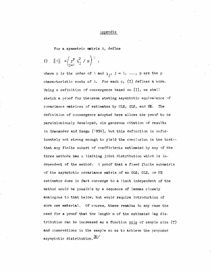
:"'ppendix
For a symmetric matrix A, define
'tlhere p is the :>rder of ~. and A.' ,j = 1, ... , p are the p J
characteristic roots of A. For each p, (r) defines a norm.
Using a definition of convergence based on (r), we shall
sketch a proof for theorems stating asymptotic equivalence :)f
covariance matrices of estimates by 018, G18, and HE. The
definition of convergence adopted here allows the proof to be
parsimioniously developed, via generous citation of results
in Grenander and Szego (1958), but this definition is unfor-
tunately not strong enough to yield the conclusion in the text--
that any finite subset of coefficients estimated by any of the
three methods has a limiting joint distribution which is in-
dependent of the method. '\ proof that a fixed finite submatrix
of the asymptotic covariance matrix of an 018, GIS, :>r HE
estimator does in fact converge to a limit independent of the
method would be possible by a sequence of lemmas closely
analogous to that below, but would require introduction of
more new materiaL Of course, there remains in any case the
need for a proof that the length m of the estimated lag dis-
tribution can be increased as a function only of sample size (T)
and observations in the sample so as to achieve the proposed
asymptotic distribution.~
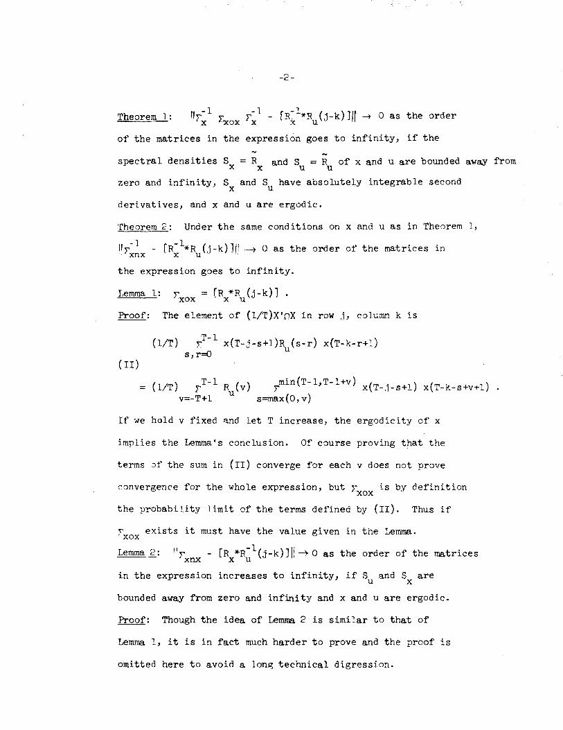
-2-
Theorem 1:
of the matrices in the expression goes to infinity, if the
-spectral densities S == Rand S == R of x and u are bounded away from x x u u
zero and infinity, Sand S have absolutely integrable second x u
derivatives, and x and u are ergodic.
Theorem 2: Under the same conditions on x and u as in Theorem 1,
n",-] - [R-l*R (j-k)]il ~ a as the order of the matrices in I Lxnx xu'
the expression goes to infinity.
Lemma 1: l,xox == [Rx*Ru(j-k)] •
Proof: The element of (l/T)X'nX in row .i, column k is
( II)
(l/T) IT-l x(T-j-s+1)R (s-r) x(T-k-r+~) u s,r=O
== (l/T) ,T-l R (v) v==-T+l u
min(T-l,T-l+v) ( ) ( ) , x T-.i-s+l x T-k-s+v+l . s=max(O,v)
If we hold v fixed and let T increase, the ergodicity of x
implies the Lemma's conclusion. Of course proving that the
terms:>f the sum in (II) converge for each v does not prove
convergence for the whole expression, but I is by definition xox
the probabi li ty limit of the terms defined by (II). Thus if
lxox exists it must have the value given in the Lemma.
Lemma 2: "lxnx - [Rx*R~l(j-k)]I! -) 0 as the order of the matrices
in the expression increases to infinity, if Sand S are u x
bounded away from zero and infinity and x and u are ergodic.
Proof: Though the idea of Lemma 2 is similar to that of
Lemma 1, it is in fact much harder to prove and the proof is
omitted here to avoid a long technical digression.
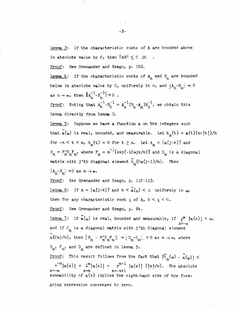
-3-
Lemma 3: If the characteristic roots of A are bounded above
in absolute value by C, then IIABIl ::; C
Proof: See Grenander and Szego, p. 103.
Lemma. 4: If the characteristic roots of A and B are bounded n n
below in absolute value by C, uniformly in n, and :IA -B i: -;. 0 p n n'
Proof: Noting that A-1-Bn-l = A-l(B -A )B- l , we obtain this
"11 n n n n
Lemma directly from Lemma 3.
Lemma 5: Suppose we have a fUnction a on the integers such
that a(w) is real, bounded, and measurable. Let b (t) = aCt )(m-It !)/m m
for -m < t < m, b (t) = 0 for t ~ m. Let A = [a(j-k)] and m m
B = F'D F , where F = m -:'"[exp( -i2TTjk/m)] and D is a diagonal m mmm m m
matrix with j'th diagonal element b (2TT(j-l)/m). Then m
i ! A - B [i -r 0 as m -1 Q). m m
Proof: See Grenander and Szego, p. 112-113.
Lemma 6: If A = [a(j-k) J and b < i(w) < c. uniformly in w,
then for any characteristic root A of A, b < A < c,
Proof: See Grenander and Szego, p. 64.
Lemma 7: If ~(w) is real, bounded and measurable, if r~ la(s)1 <~, s=-oo
and if C is a diagonal matrix with j'th diagonal element m
~(2TTj/m), then III B - F'C F II = Iii D -c Ii ~ 0 as m~ co, where m m m m ! m mli
B , F , and D are defined in Lemma 5. m m m
Proof: This result follows from the fact that Ibm (rv) - ~(w) I <
~-mla(s)1 + ~~la(s)1 + rm- l la(s)1 (Isl/m). The absolute s=-~ s=m s=-m+l summability of a(s) implies the right-hand side of the fore-
going expression converges to zero.

-4-
Henceforth we shall refer to F'C F as the "circulant mmm
approximation" to [a(j-k»).
Proof of Theorem 1: A bounded second derivative for ;:(tt)
implies (1+t2 )/a(t)/ is bounded. (This is a standard result
of Fourier analysis.) Hence the conditions of the theorem
-1 guarantee that R *R is absolutely summable, since the bounded x u
second derivatives of Sand S and the boundedness away from x u -1 zero of S guarantee that S S, the Fourier transform of x x u
R~l*Ru' has bounded second derivative. Thus from Lemma 7
[R-l*R (j-k)] differs from its circulant approximation by a x u
matrix which tends in Ii I: to zero. Applying Lemma 1 and
substituting circulant approximations for 'x and lxox' we
obtain an approximation to ,,-1 1. ~-l which is equal to x xox-x
the circulant approximation for [R-l*R (j-k)]. Lemmas 3-7 x u
now can be used in a straightforward way to show that the
difference between ,~l rxox ,~l and its approximation converges
in I! ,I to zero. This completes the proof.
Proof of Theorem 2: Lemmas 2 and 4 yield the result directly.
Footnotes
11 This is evident from frequency domain considerations.
The optimal one-step ahead forecasting scheme, assuming an
autoregressive representation exists, is given by minus the
coefficients in the autoregressive representation. The Fourier
transform of the autoregressive coefficients, squared, is the
inverse of the series' spectral density. A smooth variable
has low power at high frequencies. Hence the autoregressive
weights for such a variable must have high power at high
frequencies, making them non-smooth.
~/ The coefficients in the estimated autoregression
of fourth order were mostly individually significant. A 10th
order fit gave insignificant improvement.
~ See Nerlove (1971) or Tinsley (1971) for an explanation
of how such solutions in terms ot' future values arise.
~ Actually, this representation will fail to exist if
P has zeroes in its spectral density, as would occur were it
the first difference of a covariance-stationary process. The
cases where the representation does not exist are ,justifiably
ignored as very unlikely in most applications. But an approxima
tion to these cases, where the ratio of average to minimum
values of the spectral density is large, may not be rare in
econometric work. In such cases, though q will exist, it will
damp slowly, meaning very large samples are required for
accurate estimation. This point is closely related to one
made by Mandelbrot (1972).
-2-
21 See, e.g., Whittle (1963).
§I The "q-l" appearing in (4) is the inverse of q under
convolution. -1 If q exists at all, q exists, is unique and
is one-sided (vanishes for negative arguments).
11 This separation--a kind of certainty equivalence--is
not always possible, an important limitation to the idea which
is discussed more fUlly by Nerlove (1971).
§/ But as Shiller points out in his comment, not all
past values of a variable need be included in (8) if not all
of them appear in (10).
W The most likely class of such applications would be
situations where long lags arise out of "inertial" factors,
for example models with strong elements of persistence of habit
or with strongly increasing costs in the rate of adjustment
of a stock.
1Q/ The inefficiency of two-step procedures appears to
have been first noted by Amemiya and Fuller (1967). Specific
examples of two-step procedures are considered in detail by
Dhrymes.
111 ~ unitary matrix F is a matrix such that FF' = I.
Real unitary matrices are orthonormal. In algebra with complex
matrices it is convenient to define It,,, by F' = [fkjJ, where
f' k is the typical element of F and f kj is the complex conjugate ,)
of l' k.i·
lSI Amemiya and Fuller (1967) showed the asymptotic
equivalence of the Hannan Efficient (HE) method and GLS. The
exact equivalence becomes apparent when one realizes that
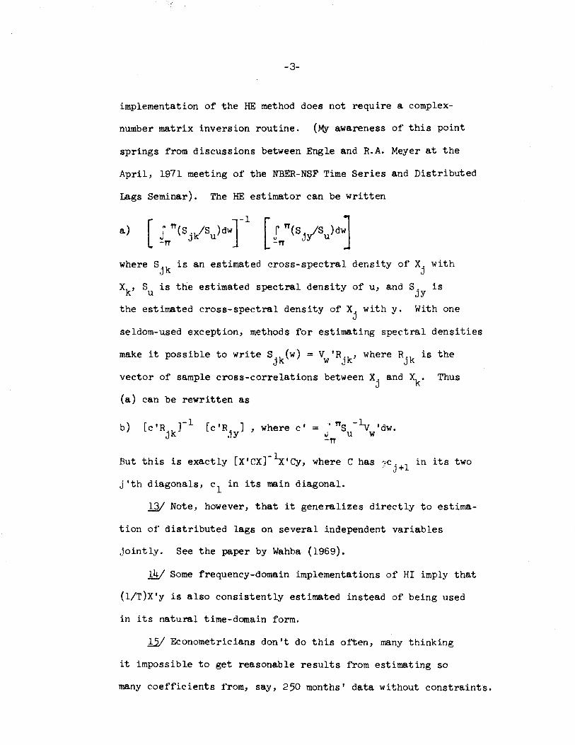
-3-
implementation of the HE method does not require a complex-
number matrix inversion routine. (My awareness of this point
springs from discussions between Engle and R.A. Meyer at the
April, 1971 meeting of the NBER-NSF Time Series and Distributed
Lags Seminar). The HE estimator can be written
where Sjk is an estimated cross-spectral density of Xj with
Xk, S is the estimated spectral density of u, and S. is u JY
the estimated cross-spectral density of Xj with y. With one
seldom-used exception, methods for estimating spectral densities
make it possible to write Sjk(w) = Yw'Rjk, where Rjk is
vector of sample cross-correlations between Xj and Xk•
(a) can be rewritten as
b) [c'R. ] , where c' JY
=' TT S -ly , dw • J u W -TT
the
Thus
But this is exactly [X'Cxr~'Cy, where C has"'-c in its two .7 j+l
j'th diagonals, cl
in its main diagonal.
~ Note, however, that it generalizes directly to estima-
tion of distributed lags on several independent variables
jointly. See the paper by Wahba (1969).
~ Some frequency-domain implementations of HI imply that
(l/T)X'y is also consistently estimated instead of being used
in its natural time-domain form.
121 Econometricians don't do this of~en, many thinking
it impossible to get reasonable results from estimating so
many coefficients from, say, 250 months' data without constraints.
-4-
As I argue below, one of the things the HI method has helped
us understand is that such estimates are feasible and useful
in many applications.
1§! See Cargill and Meyer (1972), p. 225, for one example
of such claims.
111 This applies to the standard, and most usefUl, sorts
of restrictions. However certain usefUl types of restrictions
which are not much applied because of the difficulty of im
plementing them in the time domain are easier with Fourier
methods--e.g. the requirement that the lag distribution's
Fourier transform not show sharp peaks or dips at seasonal
frequencies.
1§! Of course, the asymptotic covariance matrices used
above assume that the length of the true lag distribution
is smaller than the length of the estimated lag distribution,
so that there is no specification error. If the length of the
lag distribution were known, GLS estimates using the true length
would be more efficient than HI estimates. Even where a lag
distribution is known to be of finite length, however, which
finite length is the true one is often unknown. In this case,
it will be reasonable to expand the length of the estimated
lag distribution indefinitely as sample size increases, and
the discussion in the text is relevant. Even more often, the
lag distribution will not be known to be of finite length.
It seems likely that under fairly general conditions the three
methods, applied to finite-order approximate models whose
-5-
lag distributions increase in length with sample size, will be
equivalent in this case as well; but I can offer this only as
a "firm conjecture" at this point.
W "Filtering" a time series by "passing it through the
filter a", means replacing x by x*a. Filtering all dependent
and independent variables through the same filter does not
affect a regression relation if the independent variables are
strictly exogenous. In applied work with seasonally adjusted
quarterly aggregate data I have found, following an informal
suggestion of Nerlove, that the ad hoc filter: a(s) = 1,
-1.5, .5625, s = 0, 1, 2; a(s) = 0, s > 0 or s < 2: removes
gross serial correlation in most cases. A more complicated
filter might be required for monthly data, and of course
seasonal filtering is a subject in its own right, discussed
below.
gQJ' Lovell (1963) does suggest degrees of freedom correc-,
tions for regressions in which a moving seasonal has been removed
from the data, without explicitly recognizing the asymptotic
bias the existence of such a seasonal in the independent
variable would produce.
£1! Anyone doubting this ought to read the Federal Reserve
Board publication "Adjustment for Seasonal Variation", a reprint
from the 1941 Federal Reserve Bulletin which is still available.
The procedures described in this article are not only non-
linear, they are not functions of the raw time series. That
is, an element of manual curve fitting enters the procedures
so that the results contain a subjective element. This example
-6-
is possibly extreme and possib~r not relevant to recently
developed data series.
gg; Results shown in the initial version of this paper
did conflict with the linearity hypothesis, but correction
of a programming error brought them back into agreement with
the hypothesis.
~ Continuous time white noise is a stochastic process
such that adjacent non-overlapping averages of its values show
no serial correlation, no matter how short an interval is
chosen over which to average. Such processes do not have
numerical values at points of time.
g!V Of course a truly "unconstrained" estimate of an
infinite lag distribution is impossible, if by that we mean
an estimate which introduces no a priori information. By
"unconstrained" I really mean only "very weakly constrained';,
e.g. an estimate like the HI estimate or an OLS estimate with
a similar number of effective degrees of freedom. In appli
cations with many equations and/or many exogenous variables
relative to the number of observations the HI method and its
analogues become impractical. I would still argue that tests
of freer vs. narrower parameterizations are usetul, but in
such applications it becomes a matter of ,judgment which constraints
most need testing.
Shiller, in his comments on this paper, argues that it is
always a matter of judgment which constraints should be tested.
I agree, in the sense that I can imagine applications where
long, two-sided, linear lag distributions are not the most
-7-
interesting "unconstrained" alternative to a more tightly
parameterized model. However, there are so many types of
likely specification error which can reveal themselves in long,
two-sided estimates (misspecifications of seasonality, exo
geneity, or expectational mechanisms, for example) that where
such estimates are feasible they are generally desirable.
gj/ This point may seem too obvious to need explicit
statement. Yet we find Learner (1970) in an otherwise excellent
paper applying a carefully reasoned Bayesian analysis to the
purpose of sprucing up the appearance of two lag distributions
of length five quarters, each of which is sadly disfigured
by a strong oscillatory component, apparently statistically
significant, or frequency ~ (period 2). Since n is a seasonal
frequency, it seems very likely that bias due to seasonal noise
is the main problem with the sample estimates, not any lack
of information in the data about the lag distribution's shape.
As explained in Section 2, prior smoothness constraints may
easily increase the bias in this situation. The point is not
that Leamer's procedures are worse than those of others. His
estimates are examples; his Bayesian analysis ought to be widely
copied where theoretical justifications for smoothness assump
tions are available; and doubtless many econometricians would
have fit Koyck lag distributions to Leamer's data so that the
seasonal oscillations would never have marred their interpretations.
I myself read Leamer's paper in 1970, but noticed the oscillatory
pattern only on a recent rereading. The point is in fact, that
even the best econometric work is sometimes marred by the two
-8-
misconceptions I am attacking.
gy Cleveland (1972) takes an approach similar to Shiller's
in motivation, but arrives at a somewhat different set of
procedures.
W See Leamer (1972b) for an explanation of how these
flexible Bayesian methods may give non-obvious results when
there is bonafide multicollinearity.
gQ/ But definitely non-null. For example I have found
that filters which eliminate gross serial correlation in quarterly
aggregate quantity or value variables frequently leave price
and wage variables with substantial serial correlation.
~ Being a paraphrase in non-technical language, this
characterization of results from the paper (l97lc) is necessarily
inexact.
QQ/ In as yet unpublished work they have pursued some such
tests.
J1I They discuss distributed lag models under the name
"transfer function models" in Part III.
~ That, for fixed m, each of the estimators has an
asymptotic normal distribution with a certain covariance matrix,
and that these asymptotic covariance matrices converge to each
other, implies that there is some sequence of pairs m,T such
that the limiting distribution is achieved. But the appropriate
sequence of m,T pairs could in principle be different for each
y and x process and an appropriate m,T sequence might not be
available as a function of observable data. Thus, e.g., it
-9-
could happen that for each lower bound 6 on the spectral density
of x, an m,T sequence could be given, but that no m,T sequence
would apply f'or all positive 5. Since the lower bound on S x
cannot be known a priori, strong smoothness conditions or the
like on S '/lould be required to generate a rea] izable procedure. x
Logical problems of this nature are dealt iyith by Sims (197;c).
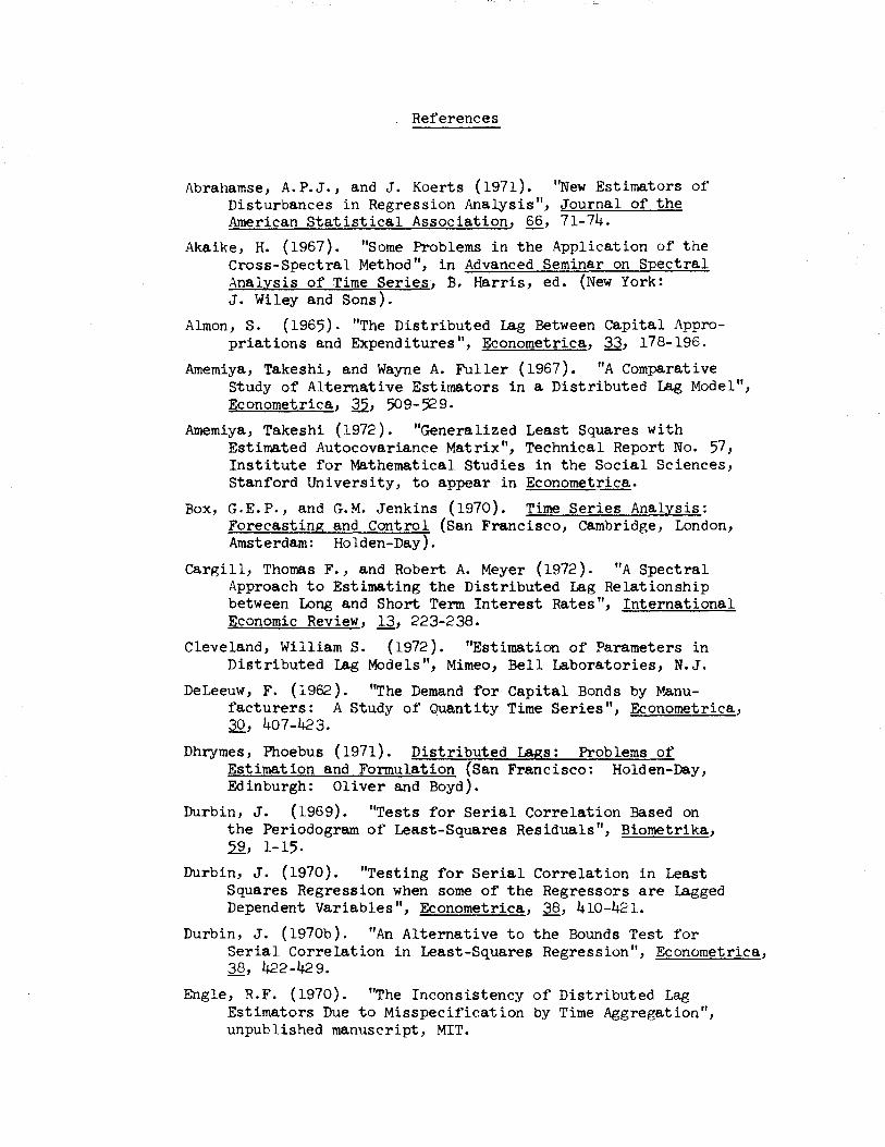
References
Abrahamse, A.P.J., and J. Koerts (1971). "New Estimators ot' Disturbances in Regression Analysis", Journal of the American Statistical Association. 66, 71-74.
Akaike, H. (1967). "Some Problems in the Application of the Cross-Spectral Method", in Advanced Seminar on Spectral Analysis of Time Series, B. Harris, ed. (New York: J. Wi ley and Sons).
Almon, S. (1965). "The Distributed Lag Between Capital Appropriations and Expenditures", Econometrica, 33, 178-196.
Amemiya, Takeshi, and Wayne A. Fuller (1967). "A Comparative Study of Alternative Estimators in a Distributed Lag Model", Econometrica, ~, 509-529.
Amemiya, Takeshi (1972). "Generalized Least Squares with Estimated Autocovariance Matrix", Technical Report No. 57, Institute for Mathematical Studies in the Social Sciences, Stanford University, to appear in Econometrica.
Box, G.E.P., and G.M. Jenkins (1970). Time Series Analysis: Forecasting and Control (San Francisco, Cambridge, London, Amsterdam: Holden-Day).
cargill, Thomas F., and Robert A. Meyer (1972). "A Spectral Approach to Estimating the Distributed Lag Relationship between Long and Short Term Interest Rates", International Economic Review, 13, 223-238.
Cleveland, William S. (1972). "Estimation of Parameters in Distributed Lag Models", Mimeo, Bell Laboratories, N.J.
DeLeeuw, F. (1962). "The Demand for Capital Bonds by M.anufacturers: A Study of Quantity Time Series", Econometrica, 30, 407-423.
Dhrymes, Phoebus (1971). Distributed Lags: Problems of Estimation and Formulation (San Francisco: Holden-Day, Edinburgh: Oliver and Boyd).
Durbin, J. (1969). "Tests for Serial Correlation Based on the Periodogram of Least-Squares Residuals", Biometrika, ,22, 1-15·
Durbin, J. (1970). "Testing for Serial Correlation in Least Squares Regression when some of the Regressors are Lagged Dependent Variables", Econometrica, 38, 410-42l.
Durbin, J. (1970b). "An Alternative to the Bounds Test for Serial Correlation in Least-Squares Regression", Econometrica, 38, 422-429.
Engle, R.F. (1970). "The Inconsistency of Distributed Lag Estimators Due to Misspecification by Time Aggregation", unpublished manuscript, MIT.
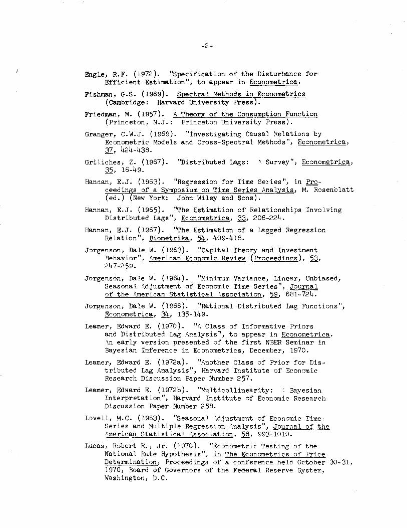
-2-
Engle, R.F. (1972). "Specification of the Disturbance for Efficient Estimation", to appear in Econometrica.
Fishman, G.S. (1969). Spectral Methods in Econometrics (Cambridge: Harvard University Press).
Friedman, M. (1957). A Theory of the Consumption Function (Princeton, N.J.: Princeton University Press).
Granger, C.W.J. (1969). "Investigating Causal Relations by Econometric Models and Cross-Spectral Methods", Econometrica, 37, 424-438.
Gri liches, Z. (1967). "Distributed Lags: '" Survey", Econometrica, ;22, 16-49.
Hannan, E.J. (1963). "Regression for Time Se:des", in Proceedings of a Symposium on Time Series Analysis, M. Rosenblatt (ed.) (New York: John Wiley and Sons).
Hannan, E.J. (1965). "The Estimation of Relationships Involving Distributed Lags", Econometrica, 33, 206-224.
Hannan, E.J. (1967). "The Estimation of a Lagged Regression Relation", Biometrika, .2!t, 409-418.
Jorgenson, Dale W. (1963). "Capital Theory and Investment Behavior", ~merican Economic Review (Proceedings), ~, 247-259.
Jorgenson, Dale w. (1964). "Minimum Variance, Linear, Unbiased, Seasona 1 :J,d.justment of Economic Time Series", Journal of the il.merican Stat lstical ~tssociation, 2ft, 681-724.
Jorgenson, Dale W. (1966). "Rational Distributed Lag Functions", Econometrica, 34, 135-149.
Leamer, Edward E. (1970). "t\. Class of Informative Priors and Distributed Lag Analysis", to appear in Econometrica. \n early version presented of the first NBER Seminar in Bayesian Inference in Econometrics, December, 1970.
Leamer, Edward E. (1972a). "Another Class of Prior for Distributed Lag Analysis", Harvard Institute of Economic Research Discussion Paper Number 257.
Leamer, Edward E. (1972b). "Multicollinearity: 'Bayesian Interpretation", Harvard Institute of Economic Research Discussion Paper Number 258.
Lovell, M.C. (1963). "Seasonal\djustment of Economic Time Series and Multiple Regression'malysis", Journal of the ;merican Statistical ~ssociation, 2§, 993-1010.
Lucas, Robert E., Jr. (1970). "Econometric Testing of the National Rate Hypothesis", in The Econometrics of Price Determination, Proceedings of a conference held October 30-31, 1970, Board of Governors of the Federal Reserve System, Washington, D.C.
-3-
Mandelbrot, Benoit (1972). "Statistical Methodology for Nonperiodic Cycles: From the Covariance to R/S Analysis", .'\nna 1 s of Economic and Socia 1 Measurement, 1, 259-290.
Moriguchi, C. (1971). "Aggregation Over Time in Macroeconomic Relations", International Economic Review, 11, 427-440.
Mundlak, Yair (1961). "Aggregation Over Time in Distributed Lag Models ", International Economic Review, ~, 154-163.
Muth, J.F. (1961). "Rational Expectations and the Theory af Price Movements", Econometrica, 29, 315-335.
Nadiri, I., and S. Rosen (1969). "Interrelated Factor Demand Functions", ·'\merican Economic Review, 22, 457-471-
Nerlove, M. (1971). "On Lags in Economic Behavior", Econometrica, 40, 221-252.
Nerlove, M., and K.F. Wallis (1966). "Use of the Durbin-',vatson Statistic in Inappropriate Situatians", Econometrica, 34, 235-238.
Pesando, James E. (1972). "Seasonal Variability in Distributed Lag Models ", Journal of the !\merican Statistical ;ssociation, 67, 311-312.
Sargan, J.D. (No date). "Some Discrete Approximations to Continuous Time Stachastic Models", to appear in the Jaurnal of the Royal Statistical Society.
Sargent, Thomas J. (1972a). "Rational Expectations and the Term Structure of Interest Rates", Journal 'Jf M'Jney, Credit and Banking, !£.
Sargent, Thomas J. (1972b). "Interest Rates and Prices in the Long Run: 'Study of the Gibson Paradox", unpublished manuscript.
Schmidt, Peter (1971). "Estimation 'Jf a Distributed Lag Model with Second-Order :\utoregressive Disturbances", International Economic Review, 12, 372-380.
Shiller, R'Jbert (1971). "l, Distributed Lag Estimator Derived from Smoothness Priors", Econ'Jmetrica, to appear. Presented at December, 1971 meetings of Econometric Society.
Shi Her, Robert (1972). Rational Exoectations and the structure of Interest Rates, unpublished Ph.D. dissertation, MIT.
Simon, H. ~,. (1953). "Causal Ordering and Identifiability", Chapter III of Studies in Ecanometric Method, 'ri. C. Hood and T. C. Koopmans ( ed . ), N e'/l York: John ',n ley and Sans.
Sims, C.'. (1971a). "Discrete ';pproximations to Continuous Time Distributed Lags in Econometrics ", Econometrica, 39, 345-554.
-4-
Sims, C. fl.. (1971b). "Approximate Specification in Distributed Lag Models". Invited paper at the 38th Session of the International Statistical Institution, Washington, D.C.
Sims, C.A. (1971c). "Distributed Lag Estimation when the Parameter Space is Explicitly Infinite-Dimensional", Annals of Mathematical Statistics, 42, 1622-1636.
Sims, C.t... (l972a). "Are There Exogenous Variables in ShortRun Production Relations?", :\nnals of Economic and Social Measurement, 1, 17-36.
Sims, C.A. (1972b). "The Role of\pproximate Prior Restricti:ms in Distributed Lag Estimation", Journal of the American Stat istical\ssociation, 67, 164-175.
Sims, C.:,. (l972c). "Money, Income and Causality", American Economic Review, 62, 540-552.
Sims, C .. \.. (1972d). "Seasonality in Regression", University of Minnesota Center for Economic Research Discussion Paper No. 23.
Sims, C.I\.. (1973). ";\ Note on Exact Tests for Serial Correlation", University of Minnesota Center for Economic Research Discussion Paper No.
Telser, Lester (l967). "Discrete Samples and Moving Sums in Stationary Stochastic Processes", Journal of the ~merican Statistical Association, 62, 484-499.
Theil, H. (1965). "The l\.nalysis of Disturbances in Regression \nalysis", Journal of the "merican Statistical ,~ssociation, 60, 1067-1079.
Thei 1, H. (1971). Principles of Econometrics (New York, London, Sydney, Toronto: John Wiley and Sons).
Thomas, J.J., and K.F. 'wallis (1971). "Seasona1 Variation in Regression Analysis", Journal of the Royal StatisticaJ S;)ciety, Series A (General), 134, 57-72.
Tinsley, P.",. (1971). "'; Variable :I,djustment MC)del 'Of Labor Demand", International Economic Review, 12, 482-510.
;,vahba, Grace (1969). "Estimation of the Coefficients in a Multidimensional Distributed Lag Model", Econometrica, 37, 398-407.
'Hallis, Kenneth F. (1972). "Seasonal \djustment and Re lat ions bet',.leen Variab les", presented to European meet ing of the Econometric S::lciety, Budapest.
Whittle, P. (1963). Prediction and Regulation by Linear Least Squares Methods, Princeton: D. Van Nostrand.
'Hymer, C.R. (1972). "Econometric Estimation o:f Stochastic Differential Equation Systems", Econometrica, 40, 565-578.
Zellner,\rnold (1966). "On the Analysis of First-Order ;\utoregressi ve Models with incomplete Data", International Economic Review, 2, 72-76.
-5-
Zellner, Arnold, and Martin S. Geisel (1970). "Analysis::>:f Distributed Lag M::>de1s with Application to C::>nsumption Function Estimation", Econometrica, 38, 865-888.
Zellner, 4rno1d, and Claude Montmarquette (1971). "\ Study o:f S::>me ~.spects o:f Temporal~,ggregatbn Problems in Econometric Analyses", Review o:f Economics and Statistics, ~, 335-342.
Recommended