Discrete Element Textures
Chongyang Ma Tsinghua University
Li-Yi Wei Microsoft Research
Xin Tong Microsoft Research Asia

Introduction
Aggregated elements in daily life

Introduction
Physics-based simulation
Physical and visual reality
Hard to control
Computationally expensive

Non-physically realistic effects
upside down
[Cho et al. 2007]
freezing elements
[Hsu & Keyser 2010]
unstable
[Cho et al. 2007]

Introduction
Physics-based simulation
Physical and visual reality
Hard to control
Computationally expensive
Manual placement
Intuitive control
Tedious
Our goals
General & flexible effects
Suitable for a variety of phenomena
May or may not be physics based
User friendly
Only need input exemplar and large scale control
Easy computation
Fast and stable

Our approach
Discrete element textures
synthesis output
control shape
input exemplar

Why?
Natural repetitions
Aggregate elements within a large-scale domain
User friendly
Direct only the large-scale domain
Avoid tedious manual work
Generality
Example-based vs. procedural
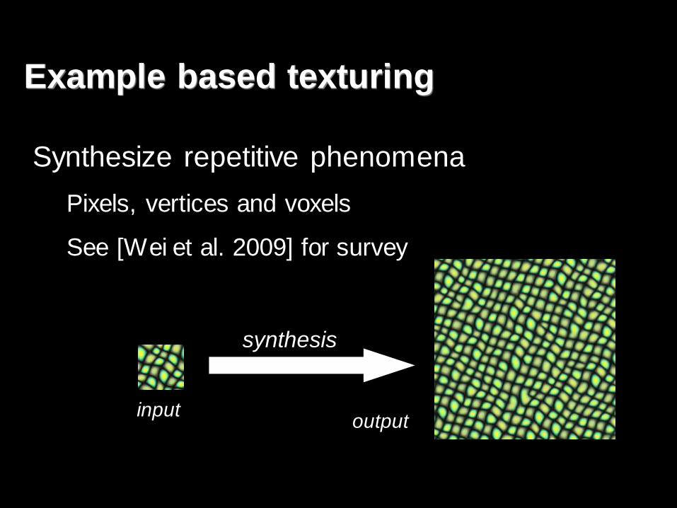
Example based texturing
Synthesize repetitive phenomena
Pixels, vertices and voxels
See [Wei et al. 2009] for survey
input output
synthesis
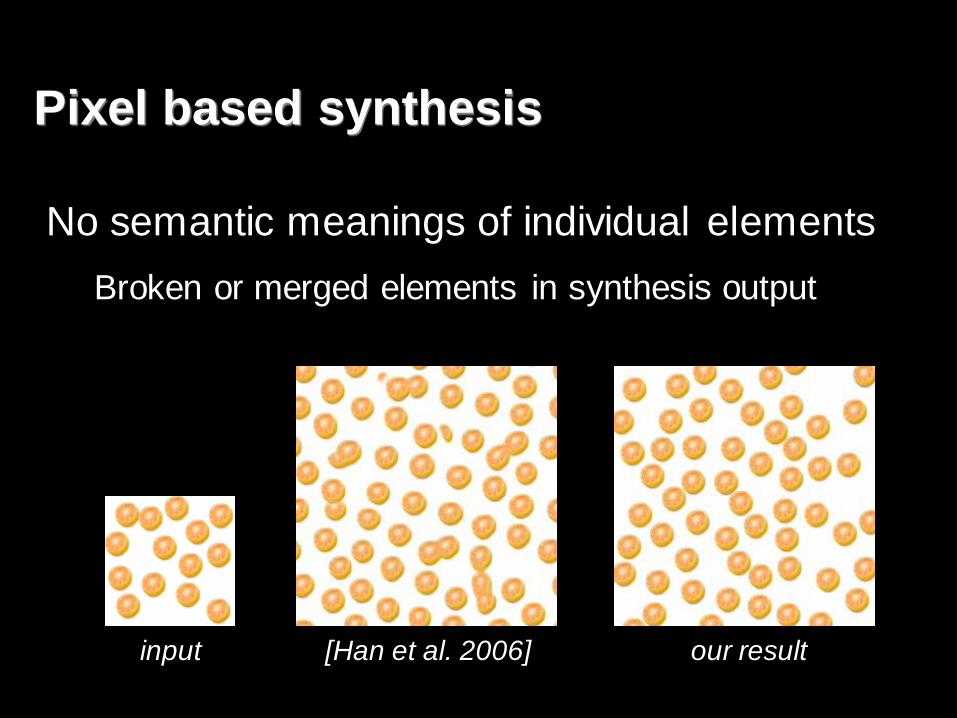
Pixel based synthesis
No semantic meanings of individual elements
Broken or merged elements in synthesis output
our result [Han et al. 2006] input

Example based element placement
Pioneering works
1D strokes [Jodoin et al. 2002]
2D elements [Dischler et al. 2002; Ijiri et al. 2008;
Hurtut et al. 2009]
2D agent motions [Lerner et al. 2007; Ju et al. 2010]
2D stipples [Kim et al. 2009; Martín et al. 2010]

Example based element placement
No robust neighborhood metric
Cannot preserve aggregate distribution
our result [Dischler et al. 2002] input

Example based element placement
Consider center positions only
Cannot handle complex element shapes
our result [Ijiri et al. 2002] input

Basic representation
Multiple samples per element
Simplicity: no need for extra orientation or shape info
Flexibility: complex and deformable shapes
banana bag spaghetti

Basic representation
Discrete element textures
𝐩 𝑠 Sample positions
𝐪 𝑠 Sample attributes (color, type, etc.)
banana bag spaghetti

Neighborhood metric
Align input and output neighborhoods
Match up the samples in pairs
output neighborhood input neighborhood
𝑠𝑖 𝑠𝑜
𝑠𝑖′
𝑠𝑜′
𝐩 𝑠𝑖′ 𝐩 𝑠𝑜
′
𝐩 𝑠𝑜′ − 𝐩 𝑠𝑖
′ 2
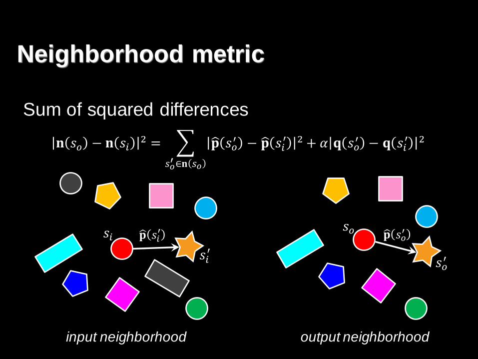
Neighborhood metric
Sum of squared differences
output neighborhood input neighborhood
𝑠𝑖 𝑠𝑜
𝑠𝑖′
𝑠𝑜′
𝐩 𝑠𝑖′ 𝐩 𝑠𝑜
′
𝐧 𝑠𝑜 − 𝐧 𝑠𝑖2 = 𝐩 𝑠𝑜
′ − 𝐩 𝑠𝑖′ 2 + 𝛼 𝐪 𝑠𝑜
′ − 𝐪 𝑠𝑖′ 2
𝑠𝑜′ ∈𝐧 𝑠𝑜

output (initialization)
Basic synthesis
Initialization via patch copy
input

Basic synthesis input
output (iteration 1)
Initialization via patch copy
Optimization based update

Basic synthesis
Convergence?
No
input
output (iteration 2)
Initialization via patch copy
Optimization based update

Basic synthesis
Convergence?
No
input
output (iteration 5)
Initialization via patch copy
Optimization based update

Basic synthesis
Convergence?
No
input
output (iteration 20)
Initialization via patch copy
Optimization based update
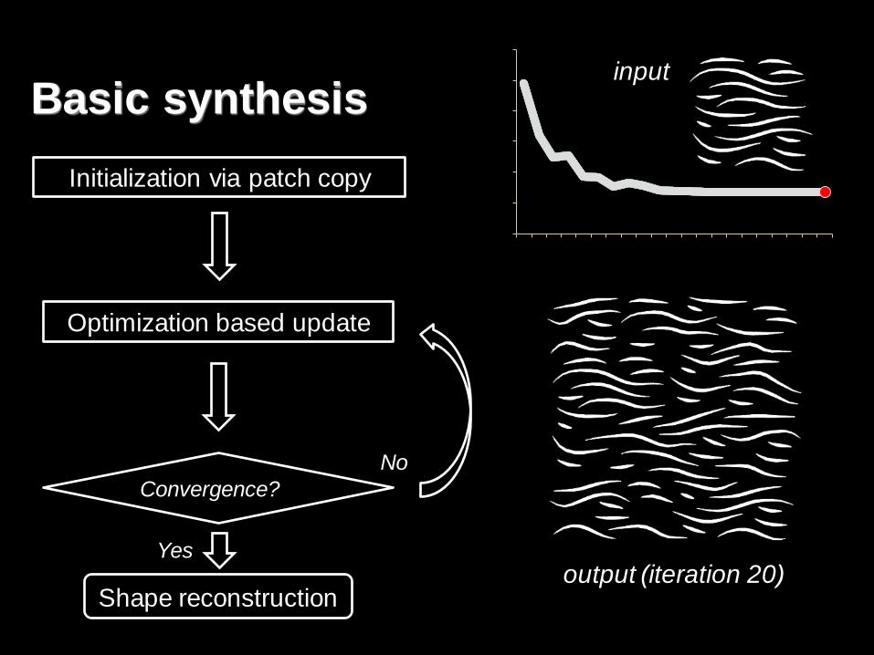
Basic synthesis
Convergence?
Yes
No
input
output (iteration 20)
Initialization via patch copy
Optimization based update
Shape reconstruction

Basic synthesis
Convergence?
Yes
No
input
output (iteration 20)
Initialization via patch copy
Optimization based update
Shape reconstruction

Basic synthesis
Convergence?
Yes
No
input
output (iteration 20)
Initialization via patch copy
Search step
Assignment step
Shape reconstruction

Search step
Find the best matching
input sample for each
output sample
Accelerate by k-coherence
search [Tong et al. 2002]
Convergence?
Yes
No
Initialization via patch copy
Search step
Assignment step
Shape reconstruction

Position assignment
Least squares from predicted offsets
𝑠𝑖 𝑠𝑜
𝑠𝑜′
𝑠𝑖′
𝐩 𝑠𝑖 − 𝐩 𝑠𝑖′
= 𝐩 𝑠𝑖 − 𝐩 𝑠𝑖′
output neighborhood input neighborhood
𝐸𝐩 𝐩 𝑠𝑜 𝑠𝑜∈𝑂= 𝐩 𝑠𝑜 − 𝐩 𝑠𝑜
′ − 𝐩 𝑠𝑜, 𝑠𝑜′ 2
𝑠𝑜′ ∈𝐧 𝑠𝑜𝑠𝑜∈𝑂
𝐩 𝑠𝑜, 𝑠𝑜′

Attribute assignment
For element/sample id, type, color, etc.
Select the vote that minimizes the energy function
Discrete solver vs. least squares
Some attributes may not be meaningfully blended
𝐪 𝑠𝑜 = argmin𝐪 𝑠𝑖 𝐪 𝑠𝑖 − 𝐪 𝑠𝑖
′ 2
𝑠𝑖′∈ 𝑠𝑖

Consider samples only during synthesis
Reconstruct elements after synthesis
Rigid bodies: shape matching
Deformable volumes: displacement interpolation
Elongated shapes: fitting with NURBS curves
Shape reconstruction

Interleaved physics solver
For common physical effects
Reduce penetrations
Obey gravity
Simulation sub-steps within each iteration
Works as an implicit energy term
Difficult to formulate explicitly
Search step
Assignment step
Simulation sub-steps

Domain shape
Constrained synthesis

Domain shape
Local orientation
Constrained synthesis

Input preparation
Procedural
Simulation
Manual work
Timing
One iteration: 5 seconds for 1000 elements
Each result: within 10 minutes
Implementation

Results

Plum stack
output
input

Pebble sculpture
output
input

Dish of corn kernels, carrots, beans
output
input

Spaghetti
output
input

More synthesis results
Spaghetti

More synthesis results
Houses

More synthesis results
Bags

Comparison
single sample per element multiple samples per element
Single-sample vs. multi-sample

Without vs. with interleaved physics solver
Comparison
without interleaved physics solver with interleaved physics solver
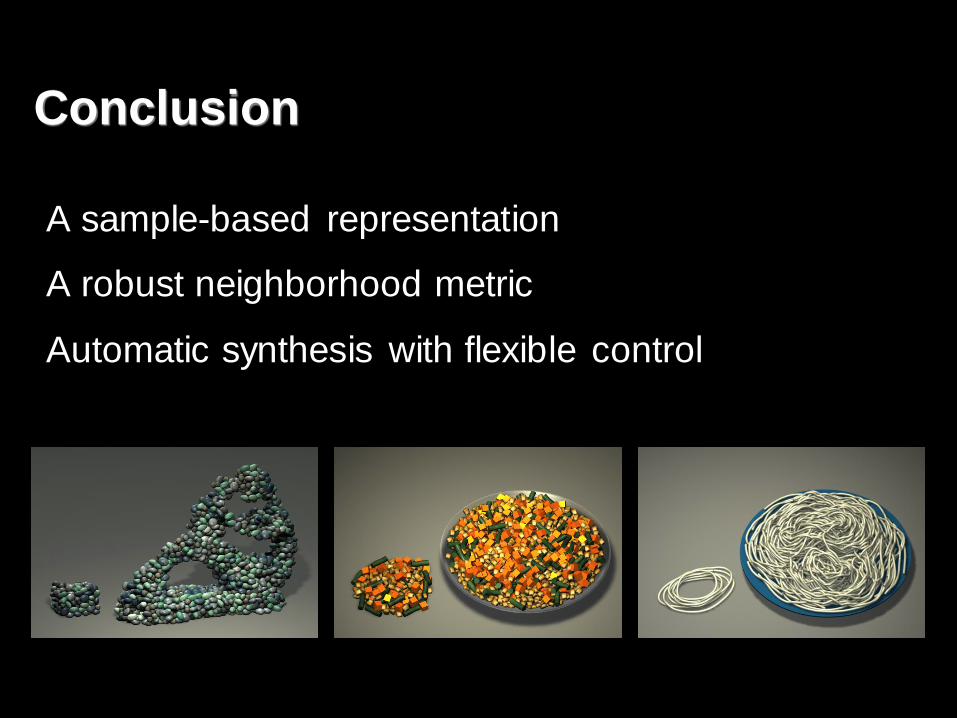
Conclusion
A sample-based representation
A robust neighborhood metric
Automatic synthesis with flexible control

Future work
Automatically obtain individual elements
2D textons [Ahuja and Todorovic 2007]
3D geometry [Pauly et al. 2008]
Minimum possible input
Summarization [Simakov et al. 2008]
Inverse synthesis [Wei et al. 2008]
Dynamic element distributions
Crowd animation [Lerner et al. 2007; Ju et al. 2010]

Acknowledgements
Weiwei Xu
Xin Sun
Stephen Lin
Matt Callcut
Yue Dong
Anonymous reviewers
Shuitian Yan
Luoying Liu
La Tu
Hongwei Li
Laras Anjung Gallery

Thank you!
Recommended