Diagnostic Fracture Injection Test (DFIT™) Analysis

Over the past few years at Halliburton we have seen a marked increase in the number of diagnostic

fracture injection tests (DFIT™) performed along with an increased desire by our customers to get this

test data analyzed and interpreted for use in planning future stimulation work and for determining

reservoir characteristics. This has lead to increased discussions about the analysis methods and

interpretation of these of tests. This article is intended to provide an overview of the information these

tests provide, present the basic analysis plots and methods used to interpret the data presented on those

plots, and provide an understanding of how the various diagnostic techniques work together in analyzing

the DFIT™ data. DFIT™ tests provide information for future fracture design and also reservoir properties

which are used for predicting future production. It is therefore critical that the test data not be

misinterpreted. This article will deal with what is referred to as Normal Leakoff Behavior. Normal leakoff

occurs with fracture closure which happens as a result of matrix leakoff after shut-in. After shut-in or

cessation of the pump-in, it is assumed the fracture stops growing. Three analysis techniques will be

looked at in this article: Nolte G-function, G-function log-log, and square-root of shut-in time. Examples

for each technique will be shown, and the various curves used to help determine closure, leakoff

mechanisms, and flow regimes will be outlined.

First we will look at Nolte G-function method, which is the most commonly used pressure decline analysis

technique. It accounts for mass conservation and fracture compliance and inherently assumes that the

rate of pressure decline is proportional to the leakoff rate.

Figure 1 - Nolte G-function analysis technique, Normal leakoff behavior

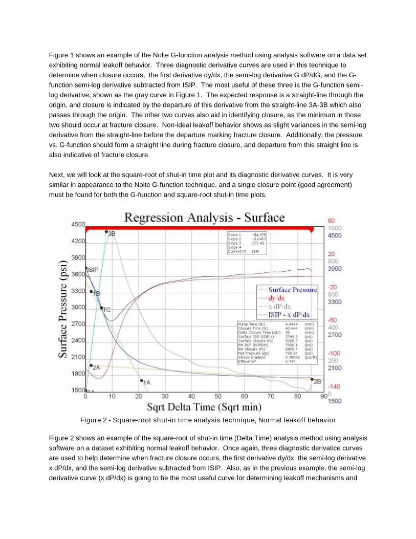
Figure 1 shows an example of the Nolte G-function analysis method using analysis software on a data set

exhibiting normal leakoff behavior. Three diagnostic derivative curves are used in this technique to

determine when closure occurs, the first derivative dy/dx, the semi-log derivative G dP/dG, and the G-

function semi-log derivative subtracted from ISIP. The most useful of these three is the G-function semi-

log derivative, shown as the gray curve in Figure 1. The expected response is a straight-line through the

origin, and closure is indicated by the departure of this derivative from the straight-line 3A-3B which also

passes through the origin. The other two curves also aid in identifying closure, as the minimum in those

two should occur at fracture closure. Non-ideal leakoff behavior shows as slight variances in the semi-log

derivative from the straight-line before the departure marking fracture closure. Additionally, the pressure

vs. G-function should form a straight line during fracture closure, and departure from this straight line is

also indicative of fracture closure.

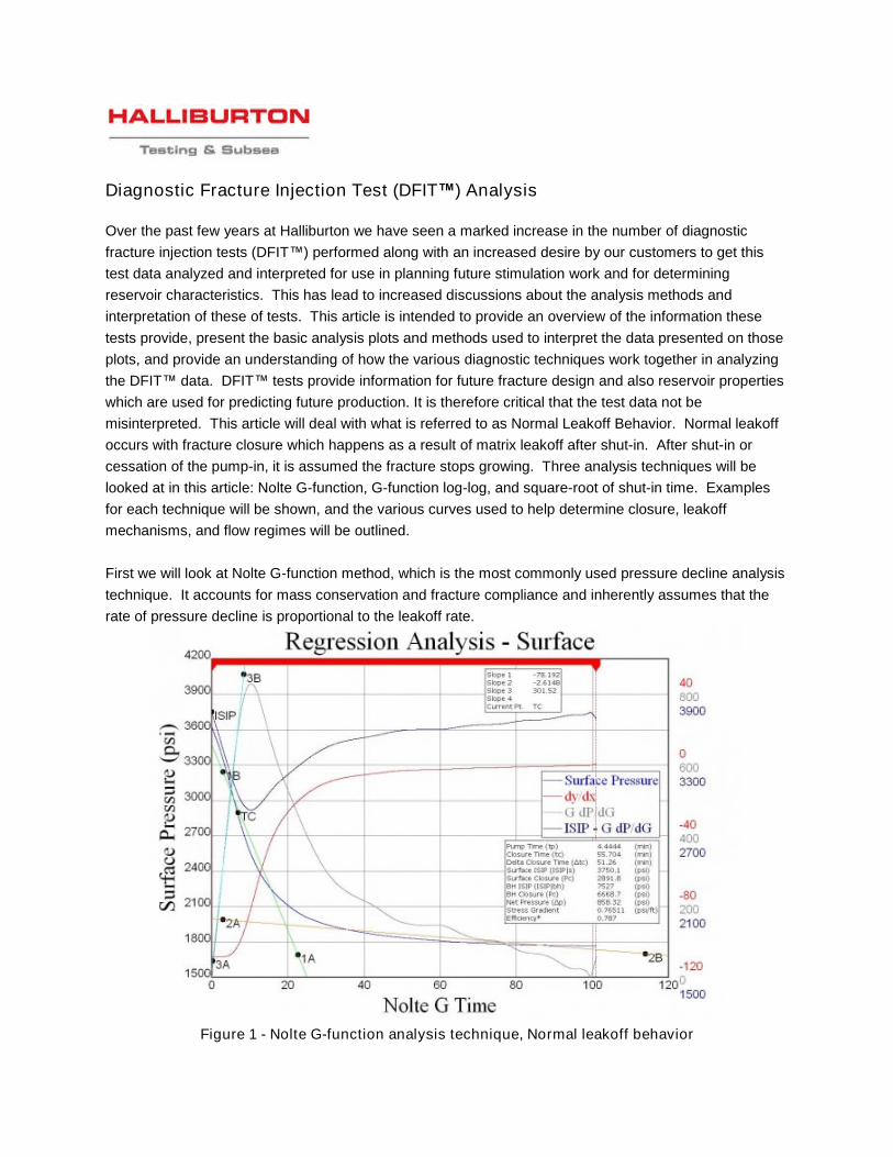
Next, we will look at the square-root of shut-in time plot and its diagnostic derivative curves. It is very

similar in appearance to the Nolte G-function technique, and a single closure point (good agreement)

must be found for both the G-function and square-root shut-in time plots.

Figure 2 - Square-root shut-in time analysis technique, Normal leakoff behavior

Figure 2 shows an example of the square-root of shut-in time (Delta Time) analysis method using analysis

software on a dataset exhibiting normal leakoff behavior. Once again, three diagnostic derivatice curves

are used to help determine when fracture closure occurs, the first derivative dy/dx, the semi-log derivative

x dP/dx, and the semi-log derivative subtracted from ISIP. Also, as in the previous example, the semi-log

derivative curve (x dP/dx) is going to be the most useful curve for determining leakoff mechanisms and

closure time/pressure. This curve is going to be equivalent to the semi-log derivative of the G-function in

low permeability cases, which is generally the type of wells to which these tests are being applied. Just

as before, closure occurs at the departure of the semi-log derivative from the straight line 3A-3B. The

other derivatives once again should be at a minimum at closure, allowing for further confirmation of the

closure pick. Like the G-function analysis the pressure vs Sqrt. Shut-in Time should form a straight line

during fracture closure; however unlike the G-function analysis fracture closure is not marked by the

departure from that straight line trend. This would lead to a later closure time and lower closure

pressure. Rather the inflection point on the pressure vs Sqrt. Shut-in Time marks closure, and is most

easily determined using the various derivative curves, particularly the first derivative where the inflection

point is determined from it by finding its maximum.

Finally, we will look at the G-function log-log analysis method. This method allows for a third confirmation

of a consistent closure point, however the greatest advantage to this method is that it allows for flow

regime identification during leakoff and after closure. This means we can determine if pseudo-linear,

pseudo-radial, or full radial flow was seen after closure, and allow us to properly analyze the after closure

data for reservoir characteristics.

Figure 3 - G-function log-log analysis technique, Normal leakoff behavior

Figure 3 shows an example of the G-function log-log analysis method using analysis software on a

dataset exhibiting normal leakoff behavior. Here we have only plotted pressure vs G-funtion and the

semi-log derivative of the G-function, G dP/dG. The flow regime before closure, the closure point, and

flow regime(s) after closure can be determined from these two curves alone, which will then allow for after

closure analysis to determine reservoir characteristics such as transmissibility (kh/µ). It can be seen that

the two curves are nearly parallel, which is usually the case immediately before closure, and the point at

which these two curves then separate marks closure. This point should be consistent (in good

agreement) with the G-function and Square root of Shut-in Time methods. The slope of these lines

before closure is indicative of the flow regime during leakoff, for example a slope of ½ is indicative of

linear flow from the fracture. After closure, the slope of the semi-log derivative curve is indicative of the

reservoir flow regime. A slope of -½ would indicate fully developed pseudo-linear flow, a slope of -1

would indicate fully developed pseudo-radial flow, and a slope of -2 would indicate fully developed radial

flow.

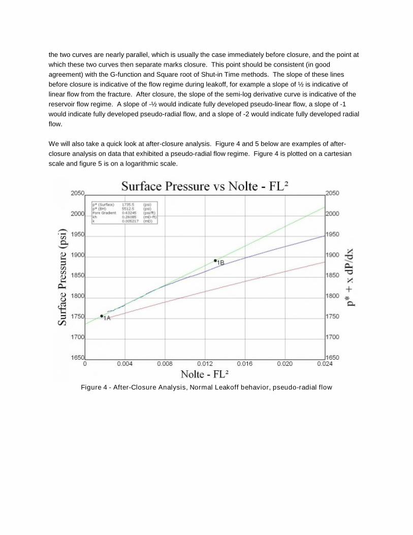
We will also take a quick look at after-closure analysis. Figure 4 and 5 below are examples of after-

closure analysis on data that exhibited a pseudo-radial flow regime. Figure 4 is plotted on a cartesian

scale and figure 5 is on a logarithmic scale.

Figure 4 - After-Closure Analysis, Normal Leakoff behavior, pseudo-radial flow

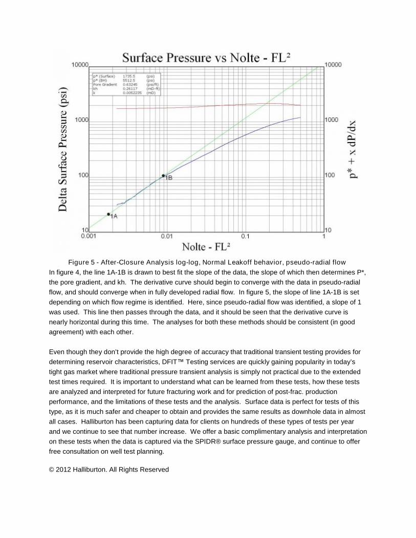
Figure 5 - After-Closure Analysis log-log, Normal Leakoff behavior, pseudo-radial flow

In figure 4, the line 1A-1B is drawn to best fit the slope of the data, the slope of which then determines P*,

the pore gradient, and kh. The derivative curve should begin to converge with the data in pseudo-radial

flow, and should converge when in fully developed radial flow. In figure 5, the slope of line 1A-1B is set

depending on which flow regime is identified. Here, since pseudo-radial flow was identified, a slope of 1

was used. This line then passes through the data, and it should be seen that the derivative curve is

nearly horizontal during this time. The analyses for both these methods should be consistent (in good

agreement) with each other.

Even though they don’t provide the high degree of accuracy that traditional transient testing provides for

determining reservoir characteristics, DFIT™ Testing services are quickly gaining popularity in today’s

tight gas market where traditional pressure transient analysis is simply not practical due to the extended

test times required. It is important to understand what can be learned from these tests, how these tests

are analyzed and interpreted for future fracturing work and for prediction of post-frac. production

performance, and the limitations of these tests and the analysis. Surface data is perfect for tests of this

type, as it is much safer and cheaper to obtain and provides the same results as downhole data in almost

all cases. Halliburton has been capturing data for clients on hundreds of these types of tests per year

and we continue to see that number increase. We offer a basic complimentary analysis and interpretation

on these tests when the data is captured via the SPIDR® surface pressure gauge, and continue to offer

free consultation on well test planning.

© 2012 Halliburton. All Rights Reserved