Depth Image Coding & Processing
Part 3: Depth Image Processing
.
Gene Cheung
National Institute of Informatics
6th July, 2015
1COST Training School 7/06/2015
Outline
• Depth Image Denoising
• Graph Sparsity Prior
• Graph-signal Smoothness Prior
• Bit-depth Enhancement
2COST Training School 7/06/2015
Outline
• Depth Image Denoising
• Graph Sparsity Prior
• Graph-signal Smoothness Prior
• Bit-depth Enhancement
3COST Training School 7/06/2015
Introduction to PWS Image Denoising
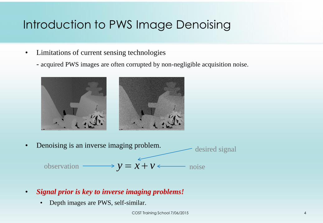
• Limitations of current sensing technologies
- acquired PWS images are often corrupted by non-negligible acquisition noise.
• Denoising is an inverse imaging problem.
• Signal prior is key to inverse imaging problems!
• Depth images are PWS, self-similar.
noise
desired signal
observation vxy
COST Training School 7/06/2015 4
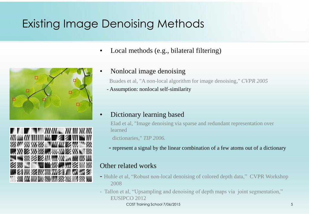
• Local methods (e.g., bilateral filtering)
• Nonlocal image denoising
Buades et al, "A non-local algorithm for image denoising," CVPR 2005
- Assumption: nonlocal self-similarity
• Dictionary learning based
Elad et al, "Image denoising via sparse and redundant representation over
learned
dictionaries," TIP 2006.
- represent a signal by the linear combination of a few atoms out of a dictionary
Other related works
- Huhle et al, “Robust non-local denoising of colored depth data,” CVPR Workshop
2008
- Tallon et al, “Upsampling and denoising of depth maps via joint segmentation,”
EUSIPCO 2012
Existing Image Denoising Methods
COST Training School 7/06/2015 5
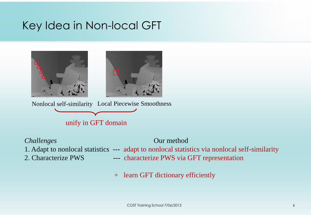
Local Piecewise SmoothnessNonlocal self-similarity
unify in GFT domain
Challenges Our method
1. Adapt to nonlocal statistics --- adapt to nonlocal statistics via nonlocal self-similarity
2. Characterize PWS --- characterize PWS via GFT representation
+ learn GFT dictionary efficiently
Key Idea in Non-local GFT
COST Training School 7/06/2015 6
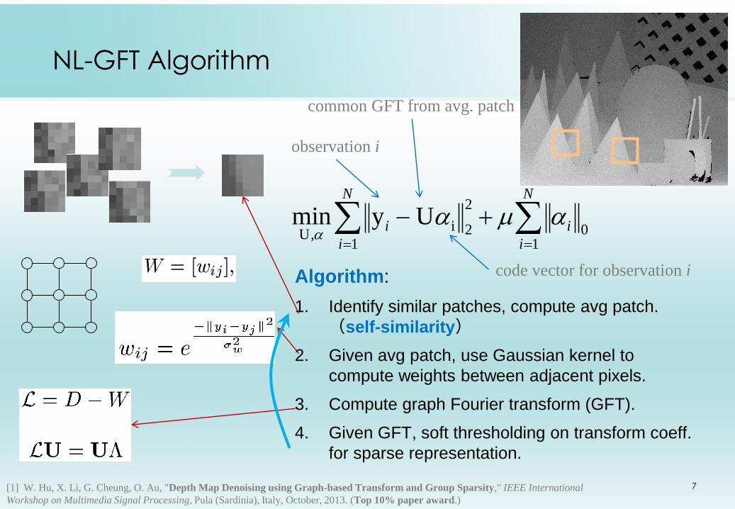
Algorithm:
1. Identify similar patches, compute avg patch.
(self-similarity)
2. Given avg patch, use Gaussian kernel to
compute weights between adjacent pixels.
3. Compute graph Fourier transform (GFT).
4. Given GFT, soft thresholding on transform coeff.
for sparse representation.
7[1] W. Hu, X. Li, G. Cheung, O. Au, "Depth Map Denoising using Graph-based Transform and Group Sparsity," IEEE International
Workshop on Multimedia Signal Processing, Pula (Sardinia), Italy, October, 2013. (Top 10% paper award.)
N
i
i
N
i
i
10
1
2
2i,U
Uymin
common GFT from avg. patch
code vector for observation i
observation i
NL-GFT Algorithm
Justification of Sparsity Prior
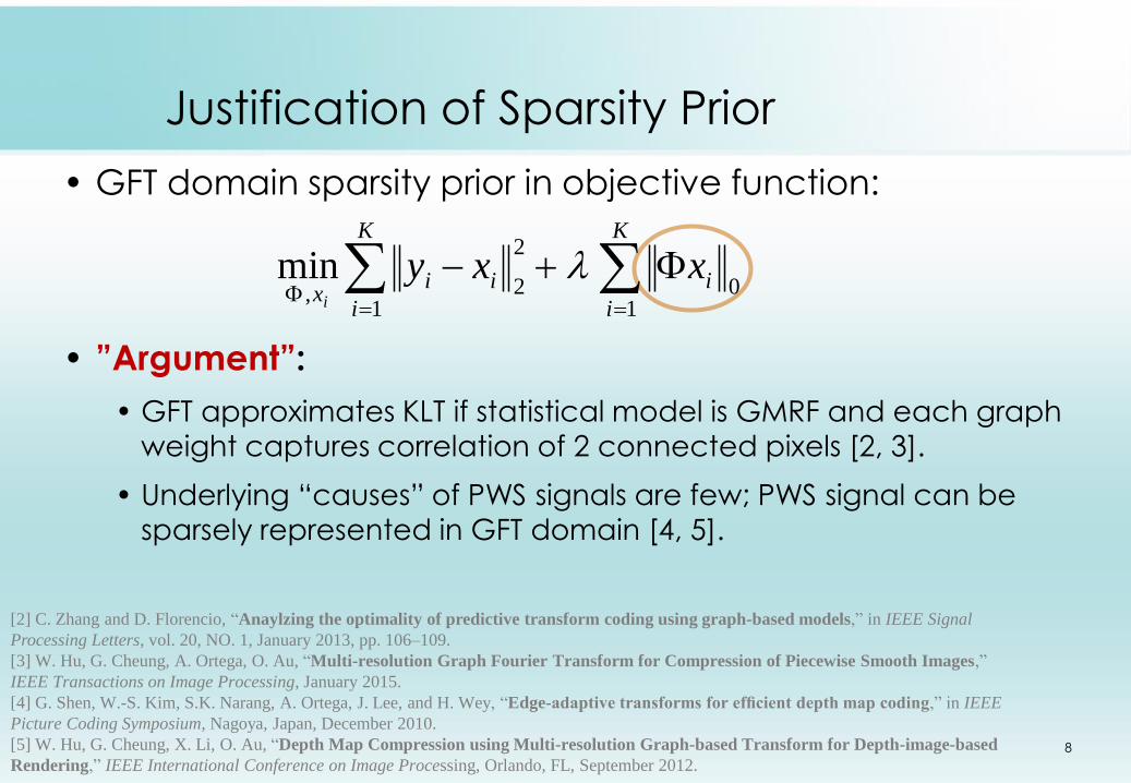
• GFT domain sparsity prior in objective function:
• ”Argument”:
• GFT approximates KLT if statistical model is GMRF and each graph
weight captures correlation of 2 connected pixels [2, 3].
• Underlying “causes” of PWS signals are few; PWS signal can be
sparsely represented in GFT domain [4, 5].
8
K
i
i
K
i
iix
xxyi 1
01
2
2,min
[2] C. Zhang and D. Florencio, “Anaylzing the optimality of predictive transform coding using graph-based models,” in IEEE Signal
Processing Letters, vol. 20, NO. 1, January 2013, pp. 106–109.
[3] W. Hu, G. Cheung, A. Ortega, O. Au, “Multi-resolution Graph Fourier Transform for Compression of Piecewise Smooth Images,”
IEEE Transactions on Image Processing, January 2015.
[4] G. Shen, W.-S. Kim, S.K. Narang, A. Ortega, J. Lee, and H. Wey, “Edge-adaptive transforms for efficient depth map coding,” in IEEE
Picture Coding Symposium, Nagoya, Japan, December 2010.
[5] W. Hu, G. Cheung, X. Li, O. Au, “Depth Map Compression using Multi-resolution Graph-based Transform for Depth-image-based
Rendering,” IEEE International Conference on Image Processing, Orlando, FL, September 2012.
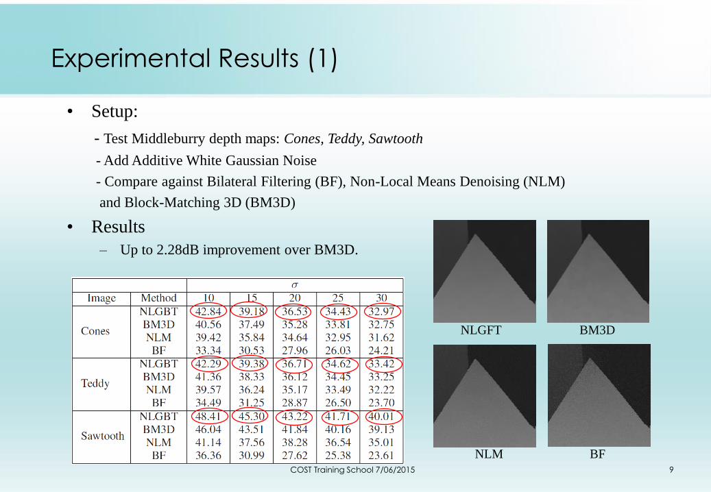
• Setup:
- Test Middleburry depth maps: Cones, Teddy, Sawtooth
- Add Additive White Gaussian Noise
- Compare against Bilateral Filtering (BF), Non-Local Means Denoising (NLM)
and Block-Matching 3D (BM3D)
• Results
– Up to 2.28dB improvement over BM3D.
NLGFT BM3D
NLM BF
Experimental Results (1)
COST Training School 7/06/2015 9
1010
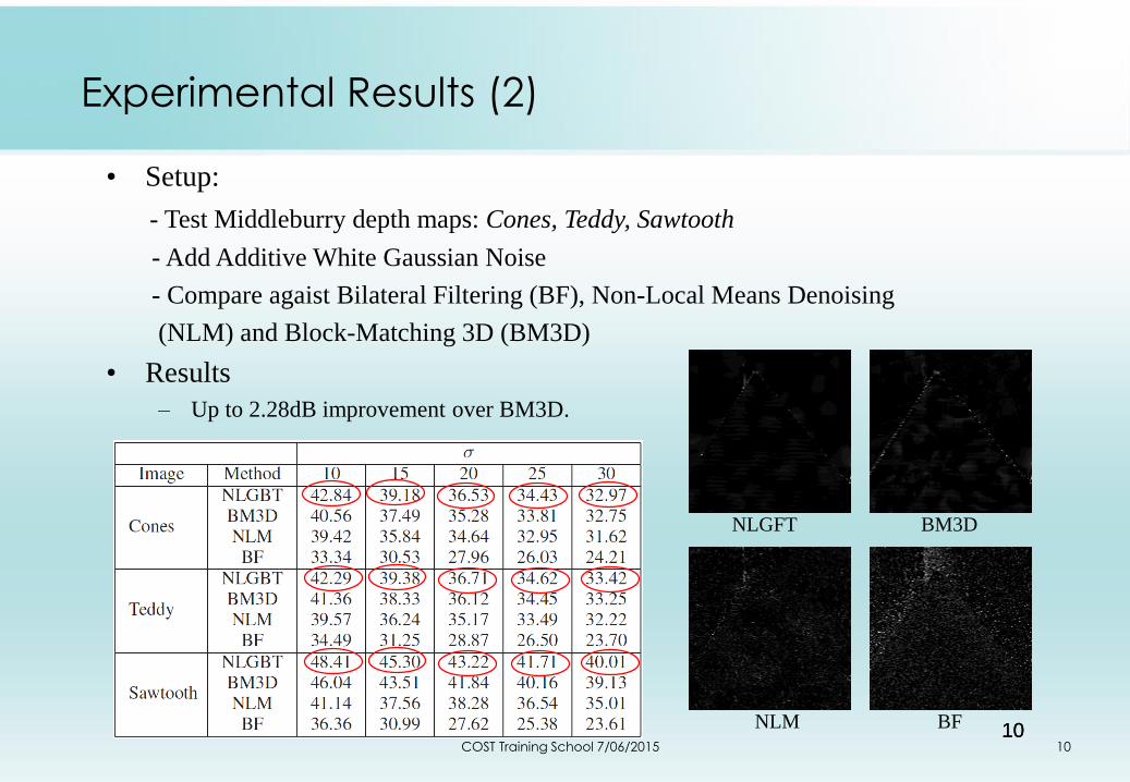
• Setup:
- Test Middleburry depth maps: Cones, Teddy, Sawtooth
- Add Additive White Gaussian Noise
- Compare agaist Bilateral Filtering (BF), Non-Local Means Denoising
(NLM) and Block-Matching 3D (BM3D)
• Results
– Up to 2.28dB improvement over BM3D.
NLGFT BM3D
NLM BF
Experimental Results (2)
COST Training School 7/06/2015 10
Outline
• Depth Image Denoising
• Graph Sparsity Prior
• Graph-signal Smoothness Prior
• Bit-depth Enhancement
11COST Training School 7/06/2015
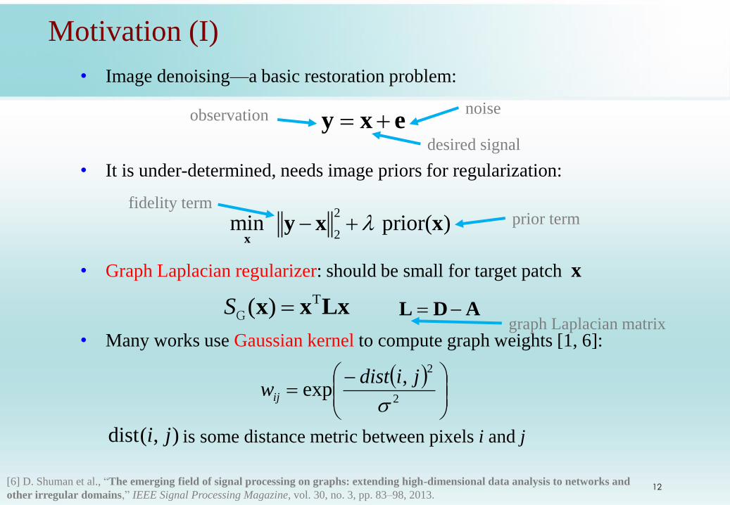
• Image denoising—a basic restoration problem:
• It is under-determined, needs image priors for regularization:
• Graph Laplacian regularizer: should be small for target patch
• Many works use Gaussian kernel to compute graph weights [1, 6]:
is some distance metric between pixels i and j
Motivation (I)
y x eobservation noise
desired signal
2
2min prior( )
xy x x
fidelity termprior term
x
T( )S x x LxG L D A
12
dist( , )i j
graph Laplacian matrix
[6] D. Shuman et al., “The emerging field of signal processing on graphs: extending high-dimensional data analysis to networks and
other irregular domains,” IEEE Signal Processing Magazine, vol. 30, no. 3, pp. 83–98, 2013.
2
2,
exp
jidistwij
approximate
discrete graph continuous manifold
Motivation (II)
13
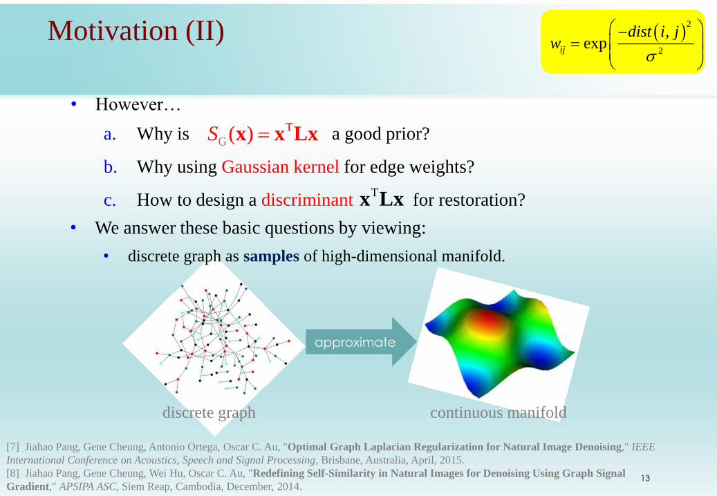
• However…
a. Why is a good prior?
b. Why using Gaussian kernel for edge weights?
c. How to design a discriminant for restoration?
T( )S x x LxG
Tx Lx
• We answer these basic questions by viewing:
• discrete graph as samples of high-dimensional manifold.
2
2
,expij
dist i jw
[7] Jiahao Pang, Gene Cheung, Antonio Ortega, Oscar C. Au, "Optimal Graph Laplacian Regularization for Natural Image Denoising," IEEE
International Conference on Acoustics, Speech and Signal Processing, Brisbane, Australia, April, 2015.
[8] Jiahao Pang, Gene Cheung, Wei Hu, Oscar C. Au, "Redefining Self-Similarity in Natural Images for Denoising Using Graph Signal
Gradient," APSIPA ASC, Siem Reap, Cambodia, December, 2014.
Our Contributions
14
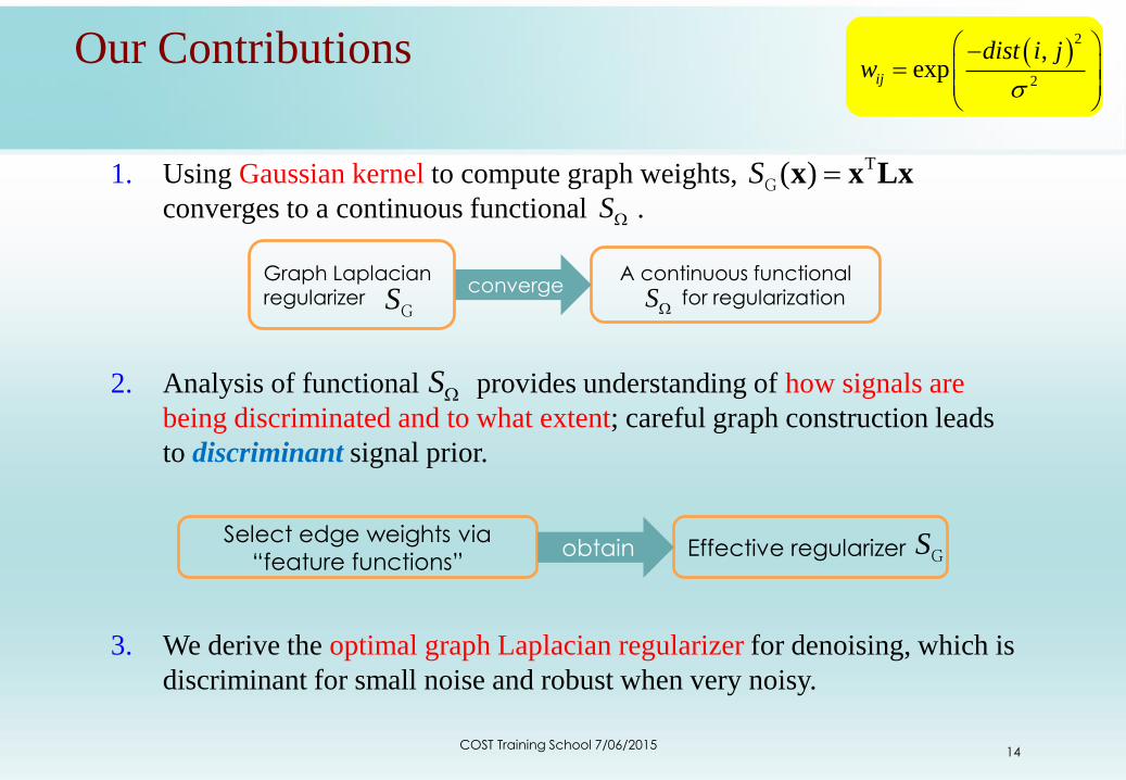
1. Using Gaussian kernel to compute graph weights,
converges to a continuous functional .
T( )S x x LxG
S
A continuous functionalfor regularization
Graph Laplacian regularizer SG S
converge
2. Analysis of functional provides understanding of how signals are
being discriminated and to what extent; careful graph construction leads
to discriminant signal prior.
S
Effective regularizer Select edge weights via
“feature functions” obtain SG
3. We derive the optimal graph Laplacian regularizer for denoising, which is
discriminant for small noise and robust when very noisy.
2
2
,expij
dist i jw
COST Training School 7/06/2015
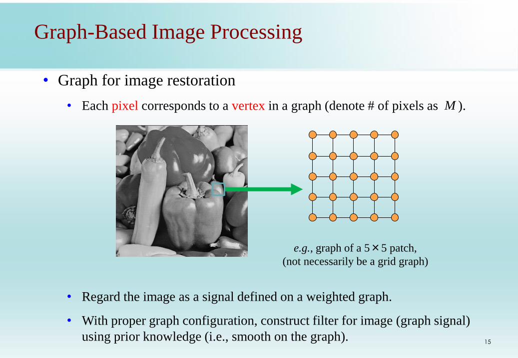
• Graph for image restoration
• Each pixel corresponds to a vertex in a graph (denote # of pixels as ).
• Regard the image as a signal defined on a weighted graph.
• With proper graph configuration, construct filter for image (graph signal)
using prior knowledge (i.e., smooth on the graph).
e.g., graph of a 5×5 patch,
(not necessarily be a grid graph)
M
Graph-Based Image Processing
15
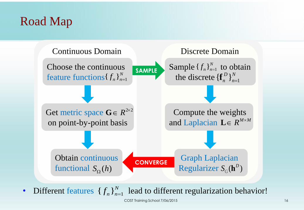
Continuous Domain Discrete Domain
Obtain continuous
functional ( )S h
Choose the continuous
feature functions 1 N
n nf
SAMPLE
Get metric space
on point-by-point basis
2 2R G Compute the weights
and Laplacian M MR L
Sample to obtain
the discrete 1 D N
n nf1 N
n nf
Graph Laplacian
Regularizer ( )DS hG
CONVERGE
• Different features lead to different regularization behavior!1 N
n nf
Road Map
COST Training School 7/06/2015 16
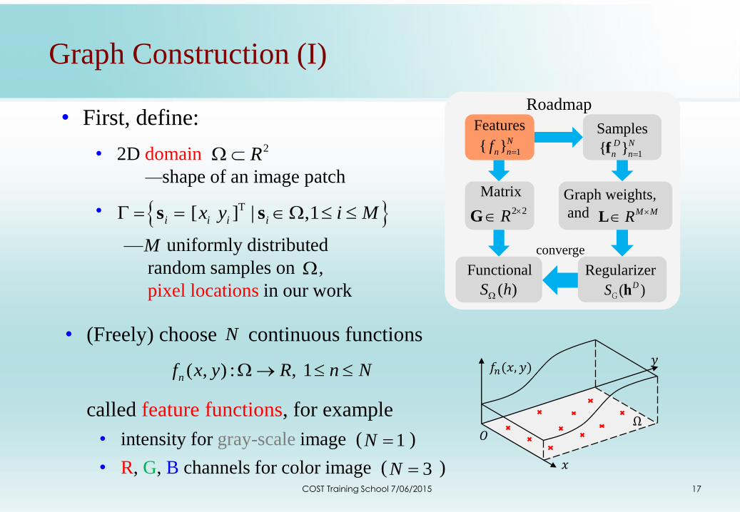
• First, define:
• 2D domain
—shape of an image patch
•
— uniformly distributed
random samples on ,
pixel locations in our work
2R
T [ ] | ,1i i i iyx i M s s
M
Functional
( )S h
Matrix
2 2R G
Graph weights,
and M MR L
Samples
1 D N
n nf1 N
n nf
Features
Regularizer
( )DS hG
converge
Roadmap
• (Freely) choose continuous functions
called feature functions, for example
• intensity for gray-scale image ( )
• R, G, B channels for color image ( )
( , ) : , 1nf x R n Ny
N
1N
3N 𝑥
𝑦𝑓𝑛(𝑥, 𝑦)
Ω𝑂
Graph Construction (I)
COST Training School 7/06/2015 17
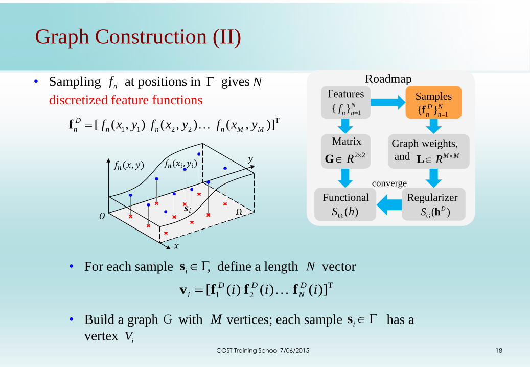
• For each sample , define a length vector
• Build a graph with vertices; each sample has a
vertex
T
1 2[ ( ) ( ) ( )]D D D
i Ni i i v f f f
i s
iV
G i s
N
M
• Sampling at positions in gives
discretized feature functions
T
1 1 2 2[ ( , ) ( , ) ( , )]D
n n MMn nf x y f x y f x y f
nf N
𝑥
𝑦𝑓𝑛(𝑥, 𝑦)
Ω𝒔𝑖
𝑓𝑛(𝑥𝑖 , 𝑦𝑖)
𝑂
Functional
( )S h
Matrix
2 2R G
Graph weights,
and M MR L
Samples
1 D N
n nf1 N
n nf
Features
Regularizer
( )DS hG
converge
Roadmap
Graph Construction (II)
COST Training School 7/06/2015 18
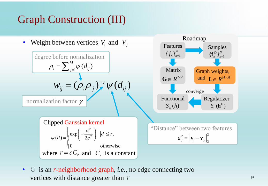
• Weight between vertices andiV jV
( ) ( )ij i j ijw d
22
2ij i jd v v
“Distance” between two features
1( )i ij
M
jd
degree before normalization
normalization factor
• is an r-neighborhood graph, i.e., no edge connecting two
vertices with distance greater than
Gr
Clipped Gaussian kernel2
2exp
2,
( )
otherwise0
dd
dr
where and is a constantrCrCr
Functional
( )S h
Matrix
2 2R G
Graph weights,
and M MR L
Samples
1 D N
n nf1 N
n nf
Features
Regularizer
( )DS hG
converge
Roadmap
Graph Construction (III)
19
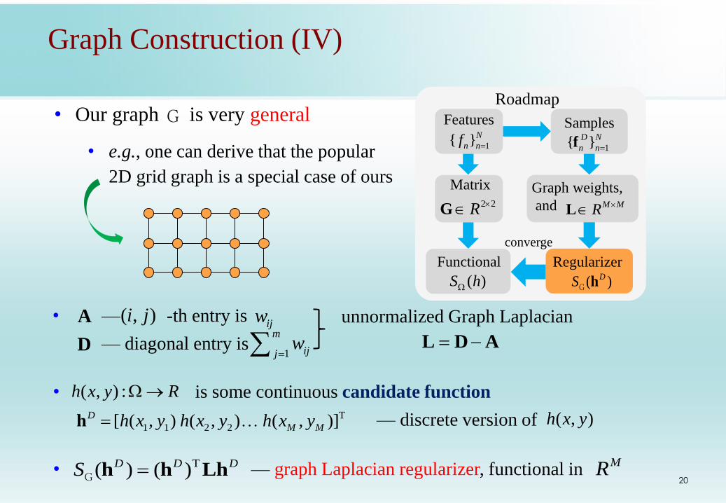
• — -th entry is
— diagonal entry is
unnormalized Graph LaplacianA ijw( , )i j
D1 ij
m
jw
L D A
• Our graph is very general
• e.g., one can derive that the popular
2D grid graph is a special case of ours
G
• — graph Laplacian regularizer, functional inT( ) ( )D D DS h h LhG
MR
• is some continuous candidate function
— discrete version of
( , ) :h x y R
T
1 1 2 2[ ( , ) ( , ) ( , )]D
M Mh x y h x y h x y h ( , )h x y
Functional
( )S h
Matrix
2 2R G
Graph weights,
and M MR L
Samples
1 D N
n nf1 N
n nf
Features
Regularizer
( )DS hG
converge
Roadmap
Graph Construction (IV)
20
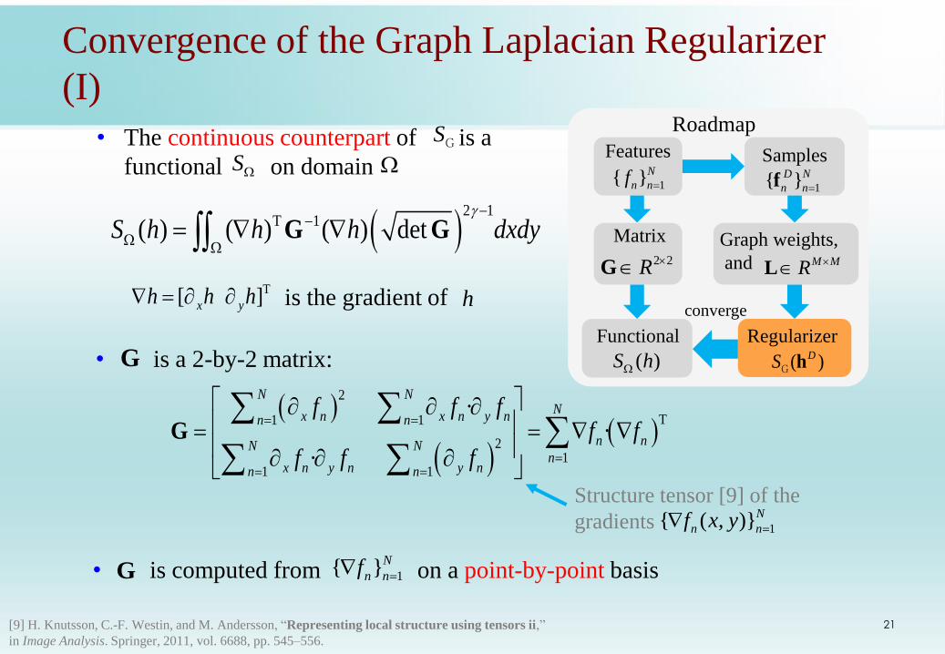
• The continuous counterpart of is a
functional on domain
is the gradient of
2 1
T 1( ) ( ) ( ) detS h h h dxdy
G G
T[ ]x yh h h h
SGS
Convergence of the Graph Laplacian Regularizer
(I)
[9] H. Knutsson, C.-F. Westin, and M. Andersson, “Representing local structure using tensors ii,”
in Image Analysis. Springer, 2011, vol. 6688, pp. 545–556.
• is a 2-by-2 matrix:
2
T1 1
2
1 11
··
·
N N
x n x n y nn n
n nN N
x n y n nn n
N
ny
f f ff f
f f f
G
Structure tensor [9] of the
gradients 1 ( , )N
n nx yf
G
• is computed from on a point-by-point basis G 1 N
n nf
Functional
( )S h
Matrix
2 2R G
Graph weights,
and M MR L
Samples
1 D N
n nf1 N
n nf
Features
Regularizer
( )DS hG
converge
Roadmap
21
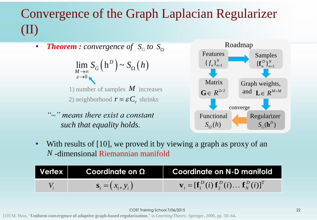
• Theorem : convergence of to
“~” means there exist a constant
such that equality holds.
2) neighborhood shrinks
SG
1) number of samples increases
S
M
Convergence of the Graph Laplacian Regularizer
(II)
[10] M. Hein, “Uniform convergence of adaptive graph-based regularization,” in Learning Theory. Springer, 2006, pp. 50–64.
• With results of [10], we proved it by viewing a graph as proxy of an
-dimensional Riemannian manifold
Vertex Coordinate on Ω Coordinate on N-D manifold
N
iV ,i i iyxsT
1 2[ ( ) ( ) ( )]D D D
i Ni i i v f f f
0
lim h ~D
GM
S S h
rCr
Functional
( )S h
Matrix
2 2R G
Graph weights,
and M MR L
Samples
1 D N
n nf1 N
n nf
Features
Regularizer
( )DS hG
converge
Roadmap
COST Training School 7/06/2015 22
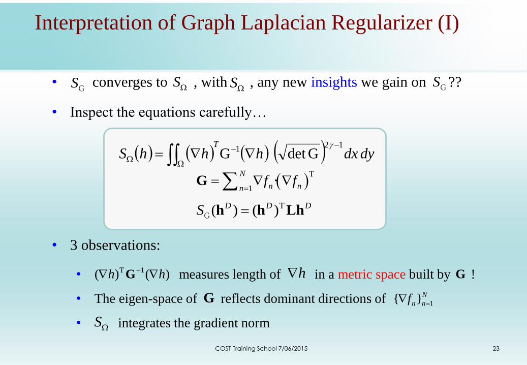
• converges to , with , any new insights we gain on ??
• Inspect the equations carefully…
• 3 observations:
• measures length of in a metric space built by !
• The eigen-space of reflects dominant directions of
• integrates the gradient norm
23
Interpretation of Graph Laplacian Regularizer (I)
SG S SGS
T 1( ) ( )h h G h
G
G
1 N
n nf
S
T
1· n
N
nnf f
G
T( ) ( )D D DS h h LhG
COST Training School 7/06/2015
dydxhhhST 12
1 GdetG

Green dots are 1 N
n nf
Justification of Graph Laplacian Regularizer (II)
• Metric space defined by ?
• At a certain location on the image
𝜕𝑥
𝜕𝑦
𝑙𝑂
G
l: dominant direction,
eigenvector corresponds to
the largest eigenvalue of G
Ellipses are contours (isolines),
reflects how concentrate 1 N
n nf
T 1( ) ( ) ( )S h h h dxdy
G T
1· n
N
nnf f
G
( , )x y
COST Training School 7/06/2015 24
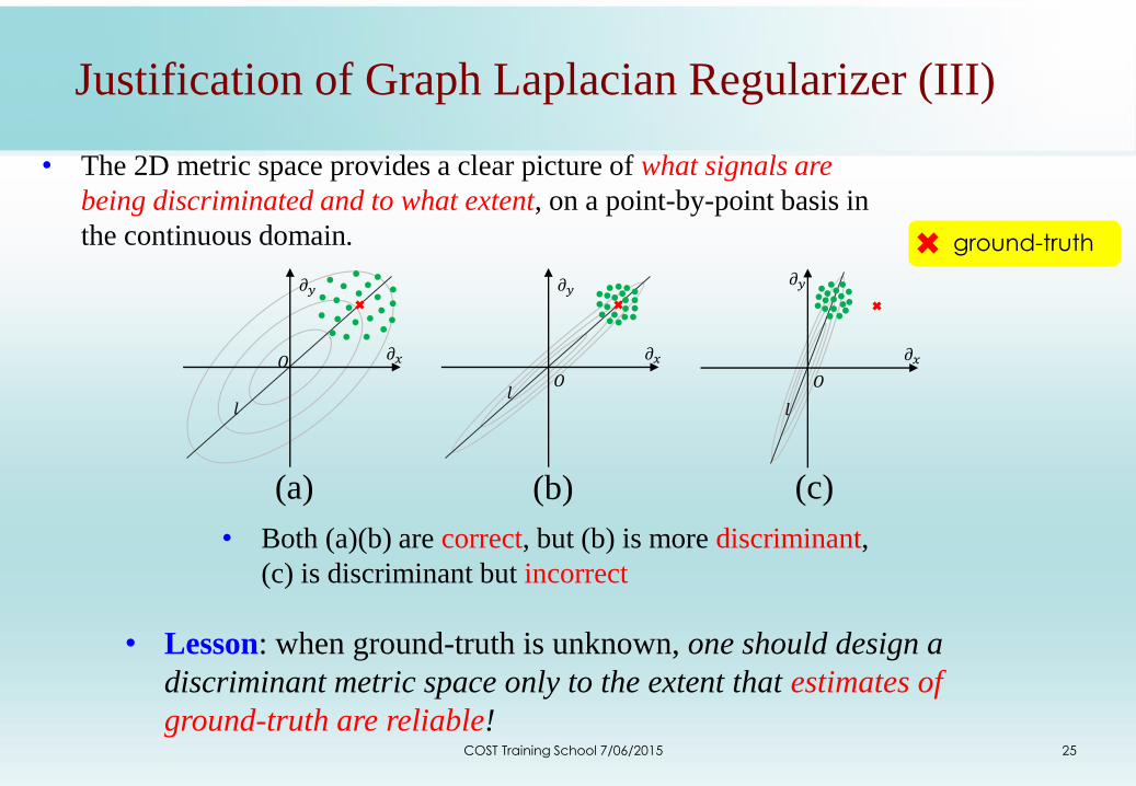
Justification of Graph Laplacian Regularizer (III)
• The 2D metric space provides a clear picture of what signals are
being discriminated and to what extent, on a point-by-point basis in
the continuous domain.
• Both (a)(b) are correct, but (b) is more discriminant,
(c) is discriminant but incorrect
• Lesson: when ground-truth is unknown, one should design a
discriminant metric space only to the extent that estimates of
ground-truth are reliable!
𝜕𝑥
𝜕𝑦
𝑙
𝑂
(a)
𝜕𝑥
𝜕𝑦
𝑙𝑂
(b)
𝜕𝑥
𝜕𝑦
𝑙
𝑂
(c)
ground-truth
COST Training School 7/06/2015 25

• For a noisy patch , identify similar patches
on the noisy image, the patches form a cluster
26
Noise Modeling in Gradient Domain
M M
2
2 2 2
1exp
2
1( | )
2k k
e e
Pr
g g g g
1K 1
0 K
k k
pK
• On patch , gradient at pixel is .
• Drop superscript , model the noisy gradients as
kp ii
kg1
0 K
k k
g
,0 1k k k K g g e
Unknown ground-truthNoise term, follows 2D Gaussian
with zero-mean and covariance
• PDF of given ground-truth (likelihood) is simply
2
e I
kg g
i
MR0p
COST Training School 7/06/2015
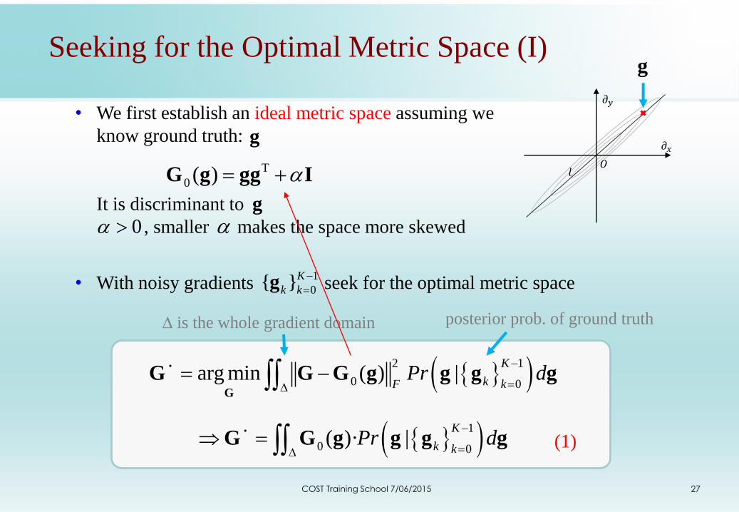
• We first establish an ideal metric space assuming we
know ground truth:
It is discriminant to
, smaller makes the space more skewed
27
Seeking for the Optimal Metric Space (I)
2 1
0 0arg min ( ) |
K
k kFPr d
G
G G G g g g g・
∆ is the whole gradient domain posterior prob. of ground truth
g
T
0 ( ) G g gg I
g
𝜕𝑥
𝜕𝑦
𝑙𝑂
g
• With noisy gradients seek for the optimal metric space
0
1
0 K
k k
g
1
0 0( )· |
K
k kdPr
G G g g g g
・(1)
COST Training School 7/06/2015
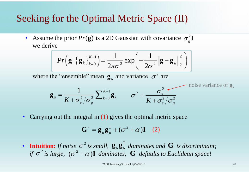
• Intuition: If noise is small, dominates and is discriminant;
if is large, dominates, defaults to Euclidean space!
• Assume the prior is a 2D Gaussian with covariance
we derive
where the “ensemble” mean and variance are
28
21
2 20 2| ex
1 1
2 2p
K
k kPr
g g g g
• Carrying out the integral in (1) gives the optimal metric space
2
T 2( ) G g g I・
( )Pr g 2
g I
g
2
1
02
1k
e g
K
kK
g g
22
2 2
e
e gK
2T
g g2 2( ) I
(2)
G・
G・
Seeking for the Optimal Metric Space (II)
COST Training School 7/06/2015
noise variance of gk
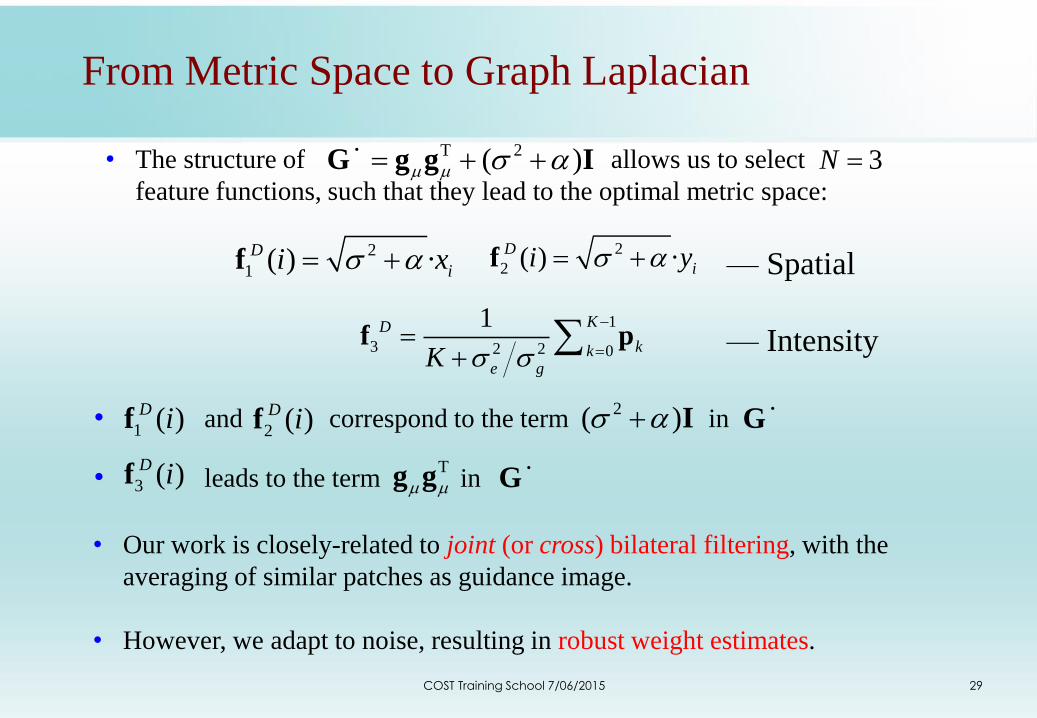
• Our work is closely-related to joint (or cross) bilateral filtering, with the
averaging of similar patches as guidance image.
• The structure of allows us to select
feature functions, such that they lead to the optimal metric space:
29
2
1 ( ) ·D
ii x f
• and correspond to the term in
2
2 ( ) ·D
ii y f
1 ( )D if
3N
03 2
1
2
1D
k
e g
K
kK
f p
2 ( )D if2( ) I G
・
• leads to the term in 3 ( )D if T
g g G・
T 2( ) G g g I・
• However, we adapt to noise, resulting in robust weight estimates.
From Metric Space to Graph Laplacian
— Spatial
— Intensity
COST Training School 7/06/2015
30
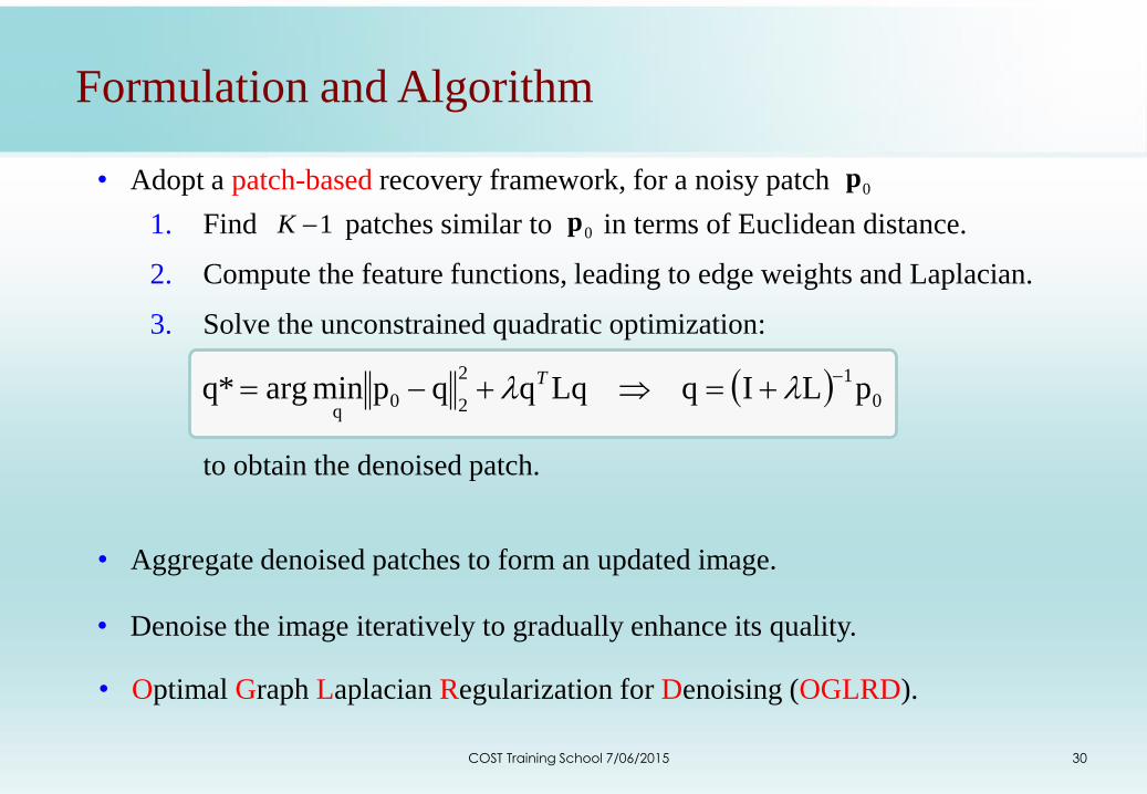
Formulation and Algorithm
• Adopt a patch-based recovery framework, for a noisy patch
1. Find patches similar to in terms of Euclidean distance.
2. Compute the feature functions, leading to edge weights and Laplacian.
3. Solve the unconstrained quadratic optimization:
to obtain the denoised patch.
0p
1K 0p
• Aggregate denoised patches to form an updated image.
• Denoise the image iteratively to gradually enhance its quality.
• Optimal Graph Laplacian Regularization for Denoising (OGLRD).
0
12
20q
pLIqLqqqpminarg*q
T
COST Training School 7/06/2015
31
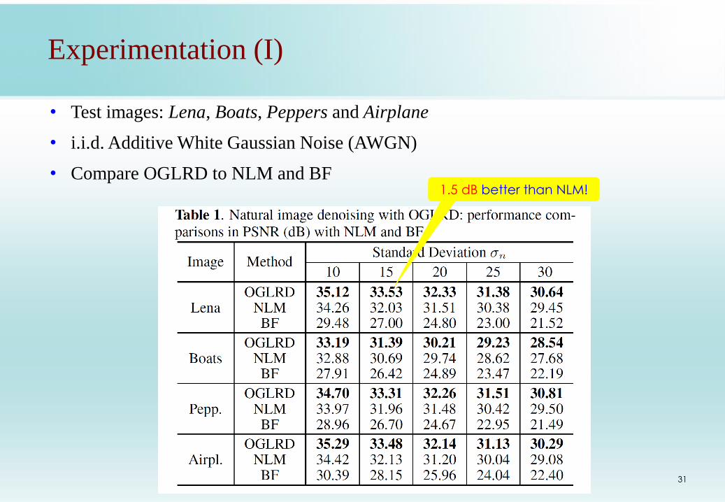
Experimentation (I)
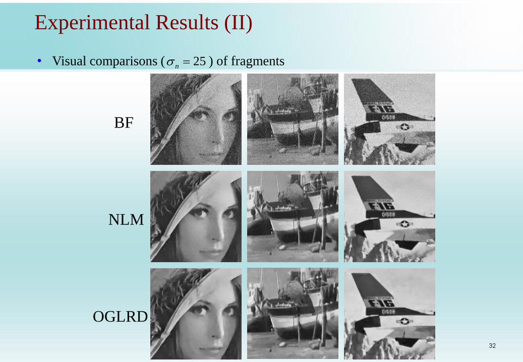
1.5 dB better than NLM!
• Test images: Lena, Boats, Peppers and Airplane
• i.i.d. Additive White Gaussian Noise (AWGN)
• Compare OGLRD to NLM and BF
32
Experimental Results (II)
• Visual comparisons ( ) of fragments25n
BF
NLM
OGLRD
33
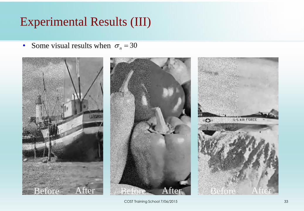
Experimental Results (III)
• Some visual results when 30n
Before After Before After Before AfterCOST Training School 7/06/2015
34
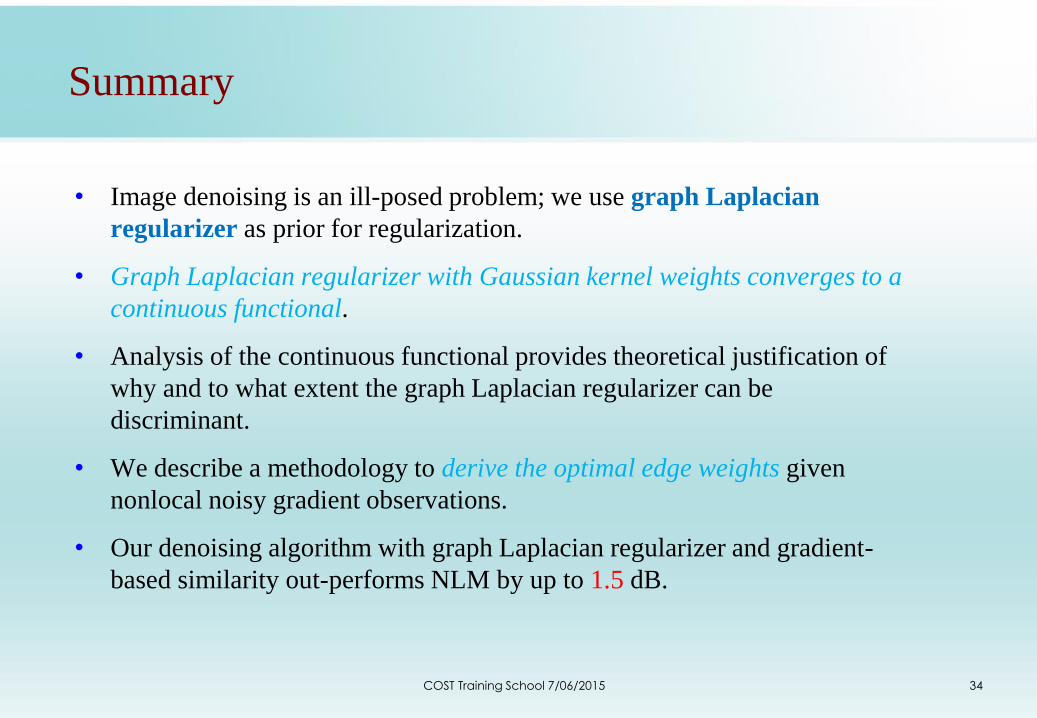
Summary
• Image denoising is an ill-posed problem; we use graph Laplacian
regularizer as prior for regularization.
• Graph Laplacian regularizer with Gaussian kernel weights converges to a
continuous functional.
• Analysis of the continuous functional provides theoretical justification of
why and to what extent the graph Laplacian regularizer can be
discriminant.
• We describe a methodology to derive the optimal edge weights given
nonlocal noisy gradient observations.
• Our denoising algorithm with graph Laplacian regularizer and gradient-
based similarity out-performs NLM by up to 1.5 dB.
COST Training School 7/06/2015
Outline
• Depth Image Denoising
• Graph Sparsity Prior
• Graph-signal Smoothness Prior
• Bit-depth Enhancement
35COST Training School 7/06/2015
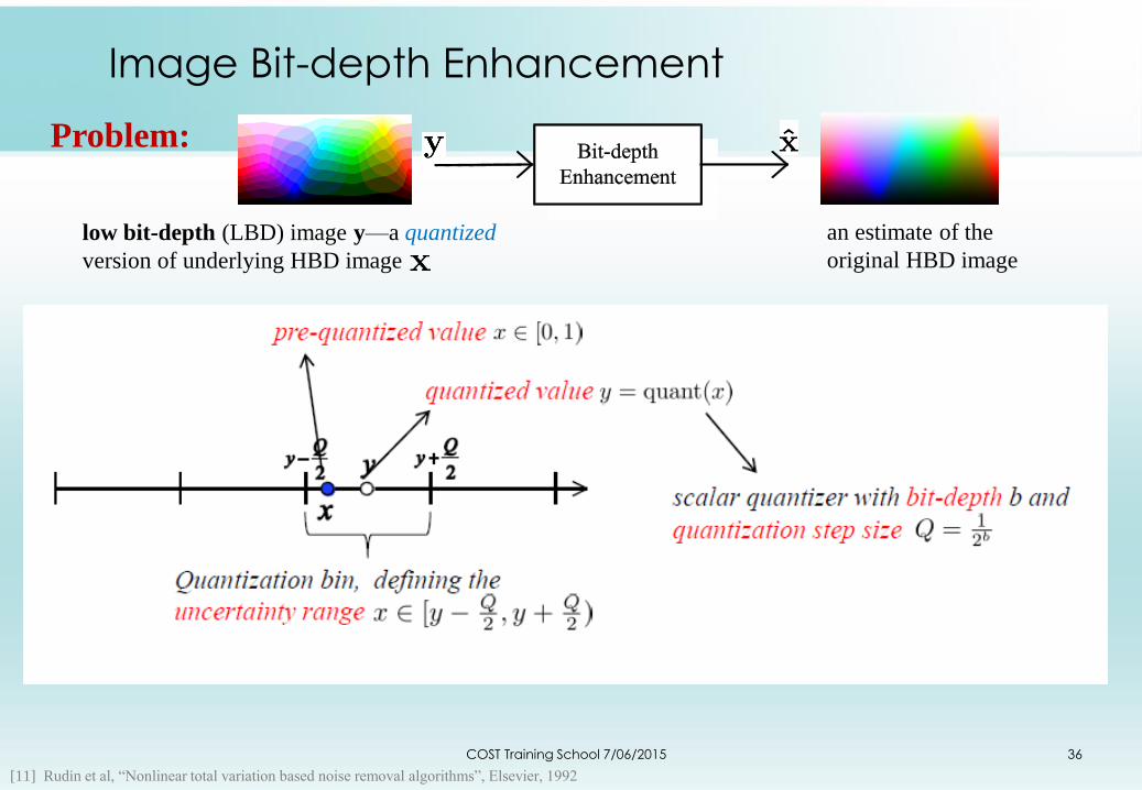
Image Bit-depth Enhancement
Problem:
low bit-depth (LBD) image y—a quantized
version of underlying HBD image
an estimate of the
original HBD image
[11] Rudin et al, “Nonlinear total variation based noise removal algorithms”, Elsevier, 1992
COST Training School 7/06/2015 36

Image Bit-depth Enhancement
Objective: find that minimizes mean-squared-error (MSE),
Smoothness prior: HBD signal is
smooth
Conventional smoothness (e.g., total Variation)
are signal-independent over-smoothing
Posterior:
Likelihood: equals to 1 iff xi quantizes
to yi
xy|xxxminargx2
2xdfMMSE
posterior prob of HBD
signal x given LBD signal y
squared errx
Question: what’s a good signal smoothness prior?
COST Training School 7/06/2015 37
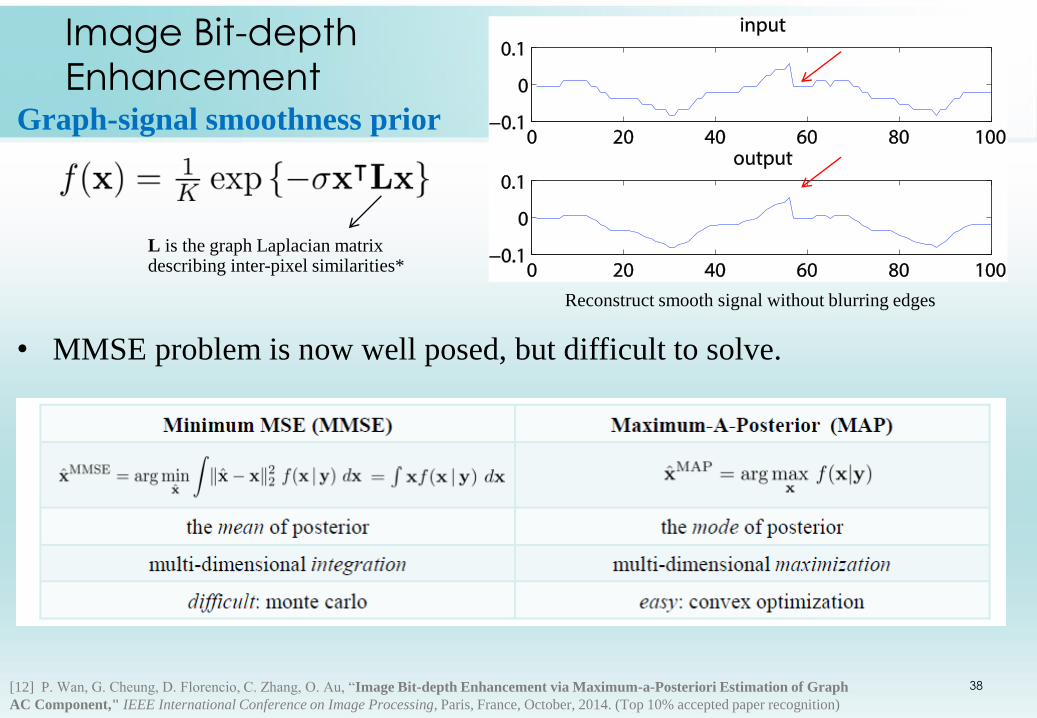
[12] P. Wan, G. Cheung, D. Florencio, C. Zhang, O. Au, “Image Bit-depth Enhancement via Maximum-a-Posteriori Estimation of Graph
AC Component," IEEE International Conference on Image Processing, Paris, France, October, 2014. (Top 10% accepted paper recognition)
Graph-signal smoothness prior
• MMSE problem is now well posed, but difficult to solve.
L is the graph Laplacian matrix describing inter-pixel similarities*
Reconstruct smooth signal without blurring edges
Image Bit-depth
Enhancement
38
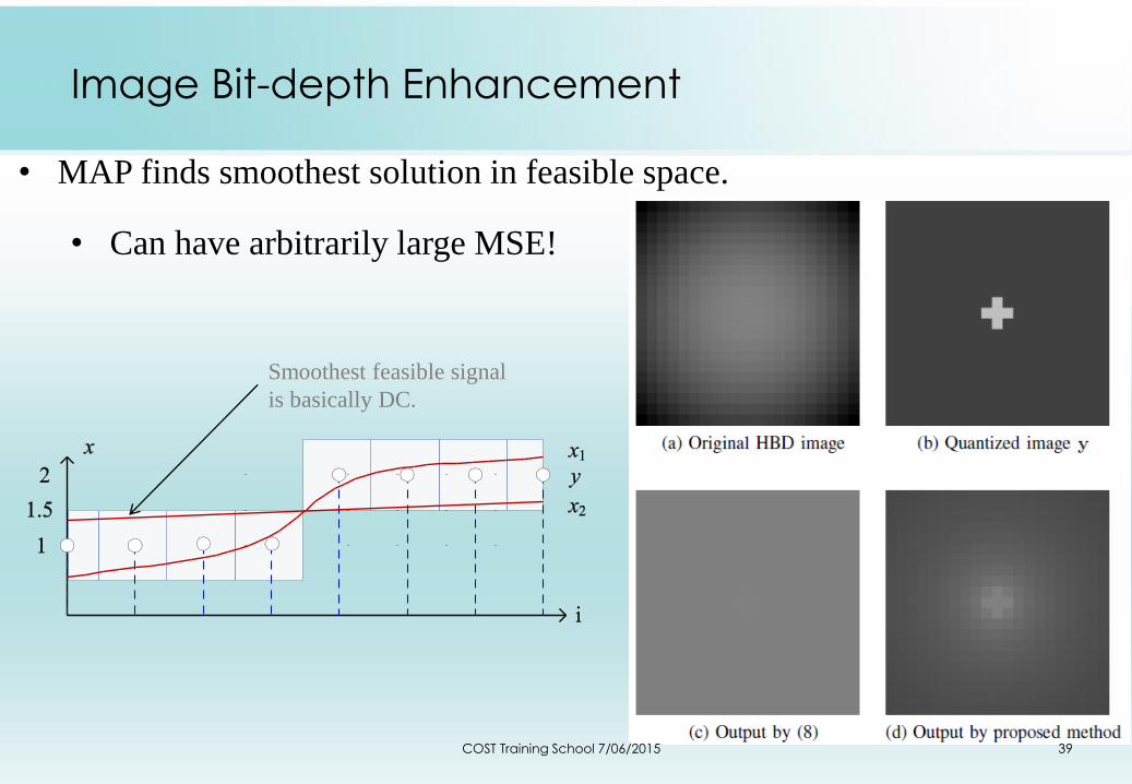
• MAP finds smoothest solution in feasible space.
• Can have arbitrarily large MSE!
Image Bit-depth Enhancement
Smoothest feasible signal
is basically DC.
COST Training School 7/06/2015 39
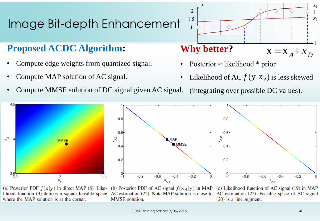
Proposed ACDC Algorithm:
• Compute edge weights from quantized signal.
• Compute MAP solution of AC signal.
• Compute MMSE solution of DC signal given AC signal.
Image Bit-depth Enhancement
Why better?
• Posterior ≈ likelihood * prior
• Likelihood of AC is less skewed
(integrating over possible DC values).
)x|y( Af
DA xxx
COST Training School 7/06/2015 40
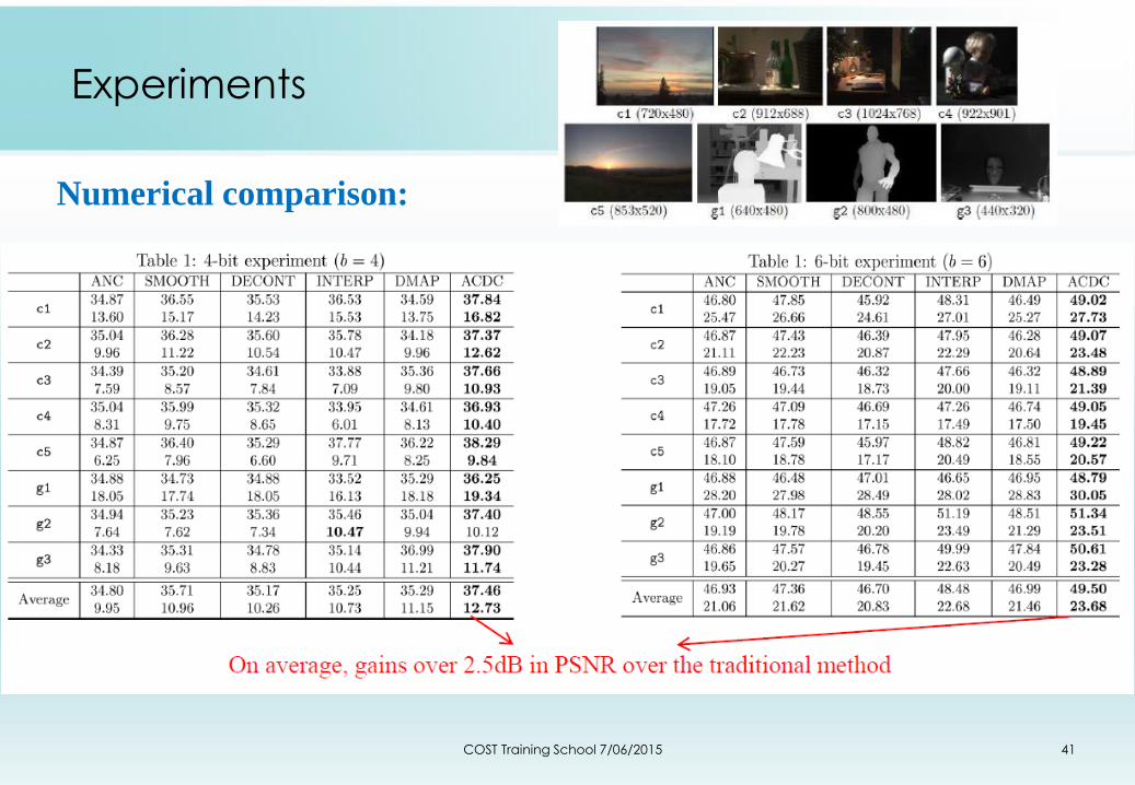
Numerical comparison:
Experiments
COST Training School 7/06/2015 41
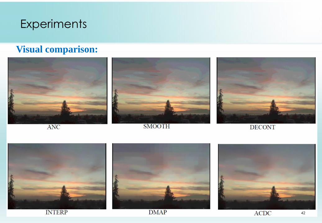
Visual comparison:
Experiments
42
Summary
• Inverse imaging requires good signal priors.
• Depth Image Denoising
• Graph Sparsity Prior (probabilistic interpretation)
• Graph-signal Smoothness Prior (deterministic interpretation)
• Bit-depth Enhancement
• Instead of fidelity term, restricted feasible space due to
quantization bin constraints (as likelihood term).
43COST Training School 7/06/2015
Conclusion
Depth Image Coding & Processing
• Coding: graph Fourier Transform (GFT), generalized graph
Fourier Transform (GGFT)
• Denoising: graph sparsity prior, graph-signal smoothness prior
Future Work
• Natural image coding using graph-based transforms.
• Depth image denoising / interpolation for non-AWGN noise.
• Apps: Given depth images, foreground / background
segmentation, tracking, face modeling, etc.
44COST Training School 7/06/2015
Recommended