Decision Diagrams for Sequencing and Scheduling
Andre Augusto Cire
Joint work with David Bergman, Willem-Jan van Hoeve, and John Hooker
Tepper School of BusinessINFORMS 2013
2
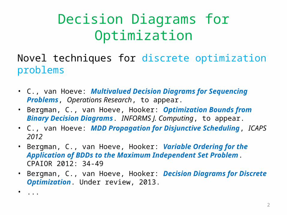
Decision Diagrams for Optimization
Novel techniques for discrete optimization problems
• C., van Hoeve: Multivalued Decision Diagrams for Sequencing Problems, Operations Research, to appear.
• Bergman, C., van Hoeve, Hooker: Optimization Bounds from Binary Decision Diagrams. INFORMS J. Computing, to appear.
• C., van Hoeve: MDD Propagation for Disjunctive Scheduling, ICAPS 2012 • Bergman, C., van Hoeve, Hooker: Variable Ordering for the Application of
BDDs to the Maximum Independent Set Problem. CPAIOR 2012: 34-49• Bergman, C., van Hoeve, Hooker: Decision Diagrams for Discrete
Optimization. Under review, 2013.• ...
3
Outline
• Definition of a decision diagram
• Application to timetable problems
• Application to disjunctive scheduling
4
What is a decision diagram?
In our context:
A decision diagram is a graphical representation of a set of solutions to a problem
5
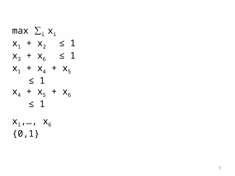
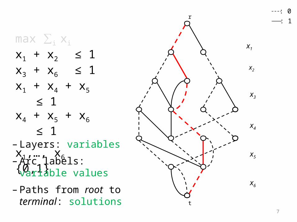
max ∑i xi
x1 + x2 ≤ 1x3 + x6 ≤ 1x1 + x4 + x5 ≤ 1x4 + x5 + x6 ≤ 1
x1,…, x6 {0,1}
6
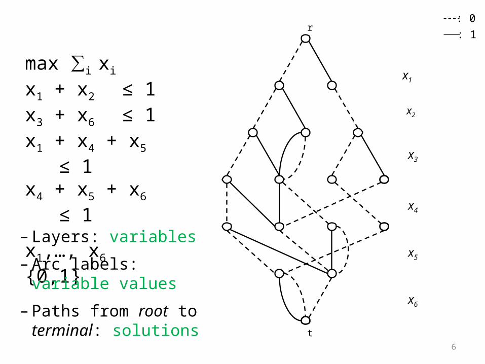
max ∑i xi
x1 + x2 ≤ 1x3 + x6 ≤ 1x1 + x4 + x5 ≤ 1x4 + x5 + x6 ≤ 1
x1,…, x6 {0,1}
r
t
x1
x2
x3
x4
x5
x6
: 0: 1
– Layers: variables
– Arc labels: variable values
– Paths from root to terminal: solutions
7
r
t
x1
x2
x3
x4
x5
x6
: 0: 1
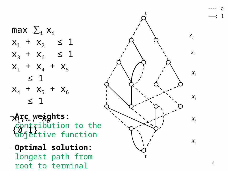
max ∑i xi
x1 + x2 ≤ 1x3 + x6 ≤ 1x1 + x4 + x5 ≤ 1x4 + x5 + x6 ≤ 1
x1,…, x6 {0,1}
– Layers: variables
– Arc labels: variable values
– Paths from root to terminal: solutions
8
r
t
x1
x2
x3
x4
x5
x6
: 0: 1
– Arc weights: contribution to the objective function
– Optimal solution: longest path from root to terminal
max ∑i xi
x1 + x2 ≤ 1x3 + x6 ≤ 1x1 + x4 + x5 ≤ 1x4 + x5 + x6 ≤ 1
x1,…, x6 {0,1}
9
r
t
x1
x2
x3
x4
x5
x6
: 0: 1
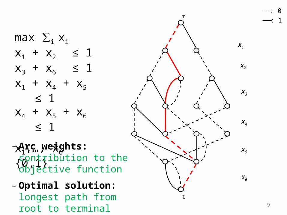
max ∑i xi
x1 + x2 ≤ 1x3 + x6 ≤ 1x1 + x4 + x5 ≤ 1x4 + x5 + x6 ≤ 1
x1,…, x6 {0,1}
– Arc weights: contribution to the objective function
– Optimal solution: longest path from root to terminal
10
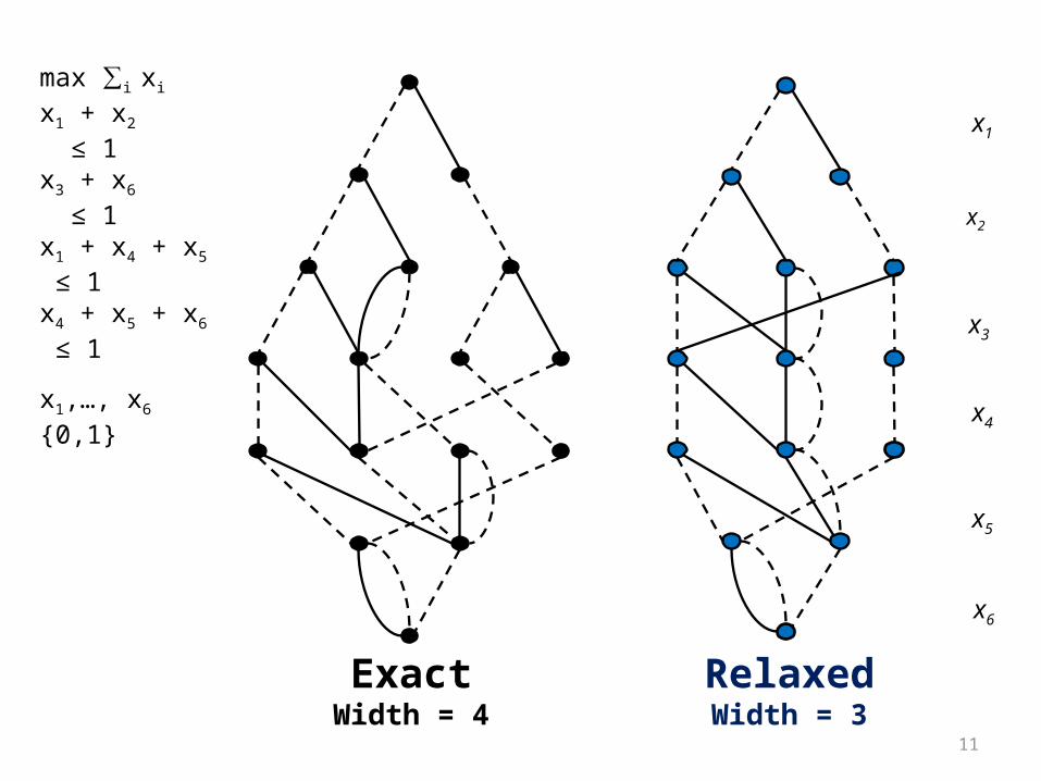
Issue
• Exactly representing all solutions requires exponentially-sized diagrams
• Alternative: Limit its size to obtain a relaxation of the set of solutions instead– Limit the width of the diagram– Strength is controlled by the width
11
RelaxedWidth = 3
ExactWidth = 4
max ∑i xi
x1 + x2 ≤ 1x3 + x6 ≤ 1x1 + x4 + x5 ≤ 1x4 + x5 + x6 ≤ 1
x1,…, x6 {0,1}
x1
x2
x3
x4
x5
x6
12
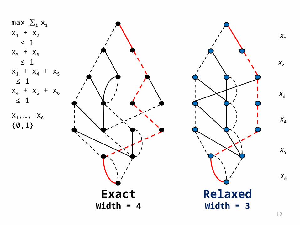
RelaxedWidth = 3
ExactWidth = 4
max ∑i xi
x1 + x2 ≤ 1x3 + x6 ≤ 1x1 + x4 + x5 ≤ 1x4 + x5 + x6 ≤ 1
x1,…, x6 {0,1}
x1
x2
x3
x4
x5
x6
13
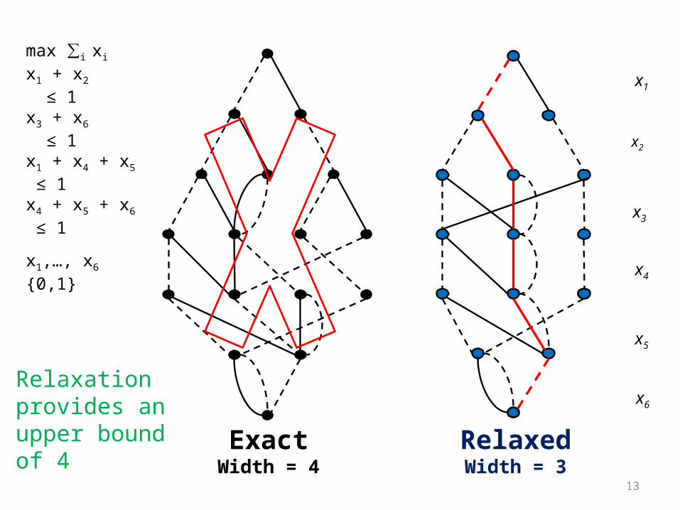
RelaxedWidth = 3
ExactWidth = 4
max ∑i xi
x1 + x2 ≤ 1x3 + x6 ≤ 1x1 + x4 + x5 ≤ 1x4 + x5 + x6 ≤ 1
x1,…, x6 {0,1}
x1
x2
x3
x4
x5
x6 Relaxation provides an upper bound of 4
14
Relaxed Diagrams
• Provide bounds on the objective function
• They can also be used for inference– Deduction of new constraints
15
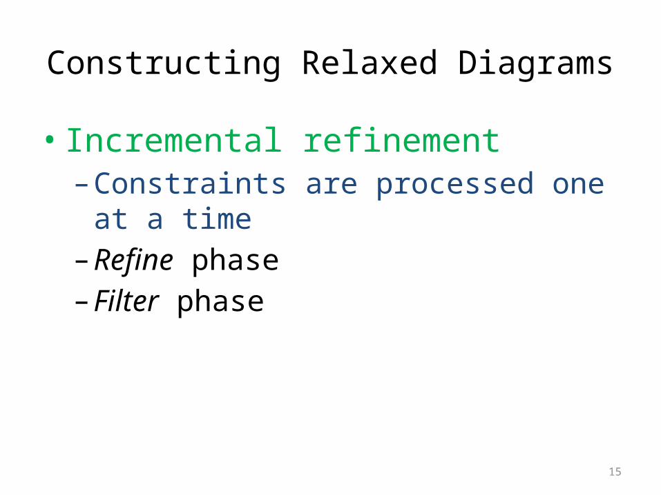
Constructing Relaxed Diagrams
• Incremental refinement– Constraints are processed one at a time– Refine phase– Filter phase
16
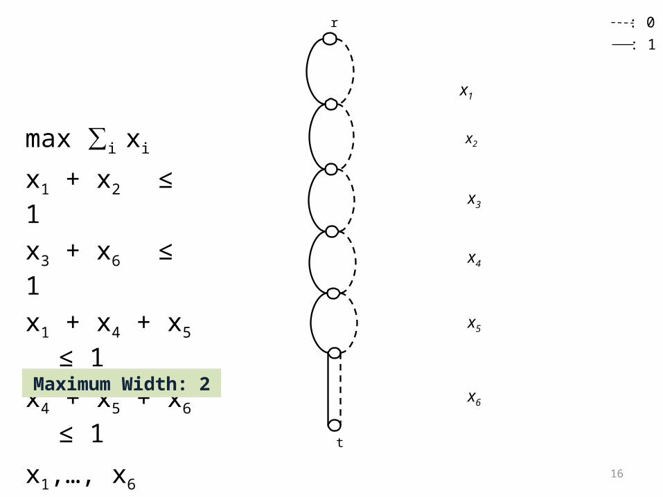
max ∑i xi
x1 + x2 ≤ 1
x3 + x6 ≤ 1
x1 + x4 + x5 ≤ 1
x4 + x5 + x6 ≤ 1
x1,…, x6 {0,1}
r : 0: 1
t
x1
x2
x3
x4
x5
x6 Maximum Width: 2
17
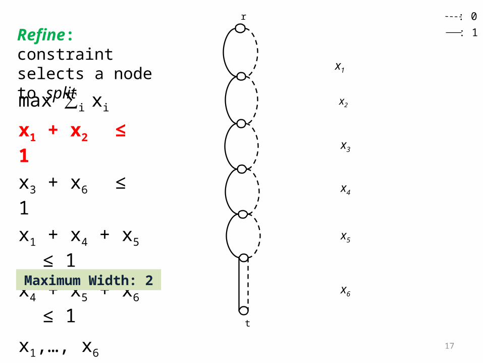
max ∑i xi
x1 + x2 ≤ 1
x3 + x6 ≤ 1
x1 + x4 + x5 ≤ 1
x4 + x5 + x6 ≤ 1
x1,…, x6 {0,1}
r
t
: 0: 1
x1
x2
x3
x4
x5
x6 Maximum Width: 2
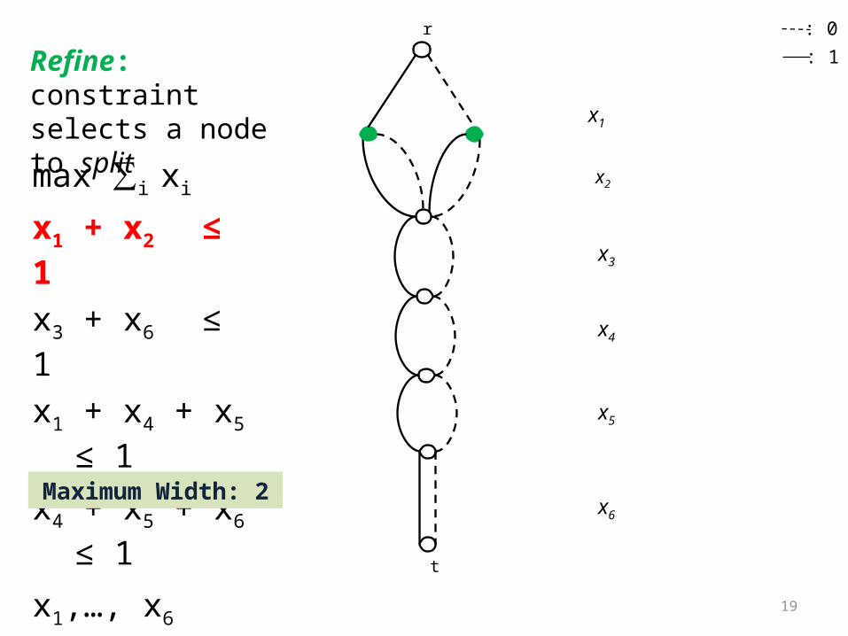
Refine: constraint selects a node to split
18
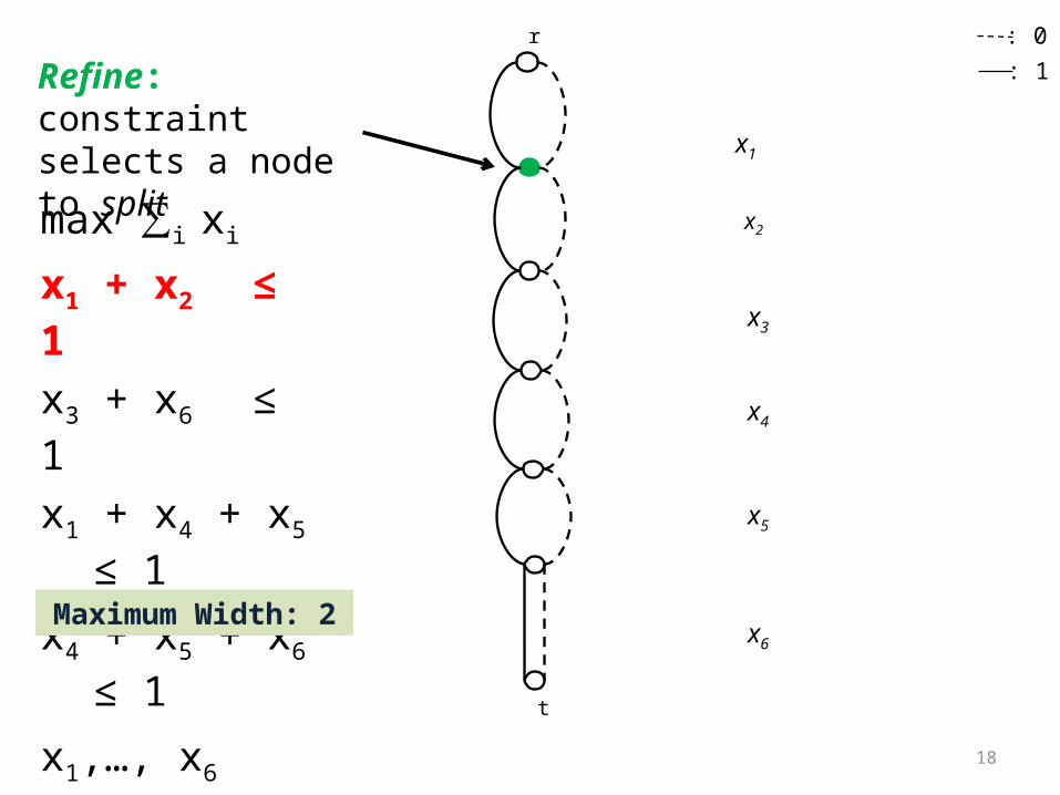
max ∑i xi
x1 + x2 ≤ 1
x3 + x6 ≤ 1
x1 + x4 + x5 ≤ 1
x4 + x5 + x6 ≤ 1
x1,…, x6 {0,1}
r
t
: 0: 1
x1
x2
x3
x4
x5
x6
Refine: constraint selects a node to split
Maximum Width: 2
19
r
t
: 0: 1
x1
x2
x3
x4
x5
x6
max ∑i xi
x1 + x2 ≤ 1
x3 + x6 ≤ 1
x1 + x4 + x5 ≤ 1
x4 + x5 + x6 ≤ 1
x1,…, x6 {0,1}
Refine: constraint selects a node to split
Maximum Width: 2
20
r
t
: 0: 1
x1
x2
x3
x4
x5
x6
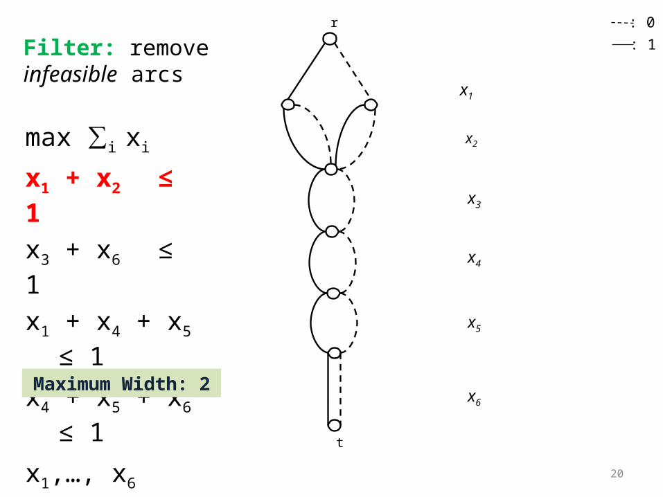
Filter: remove infeasible arcs
max ∑i xi
x1 + x2 ≤ 1
x3 + x6 ≤ 1
x1 + x4 + x5 ≤ 1
x4 + x5 + x6 ≤ 1
x1,…, x6 {0,1}
Maximum Width: 2
21
r
t
: 0: 1
x1
x2
x3
x4
x5
x6
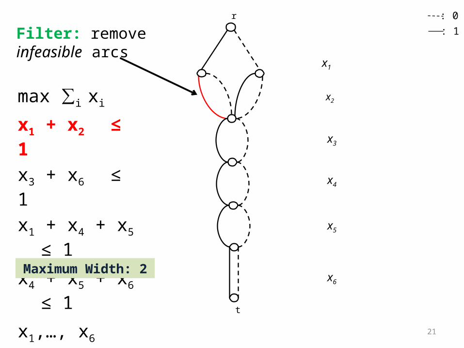
max ∑i xi
x1 + x2 ≤ 1
x3 + x6 ≤ 1
x1 + x4 + x5 ≤ 1
x4 + x5 + x6 ≤ 1
x1,…, x6 {0,1}
Filter: remove infeasible arcs
Maximum Width: 2
22
r
t
: 0: 1
x1
x2
x3
x4
x5
x6
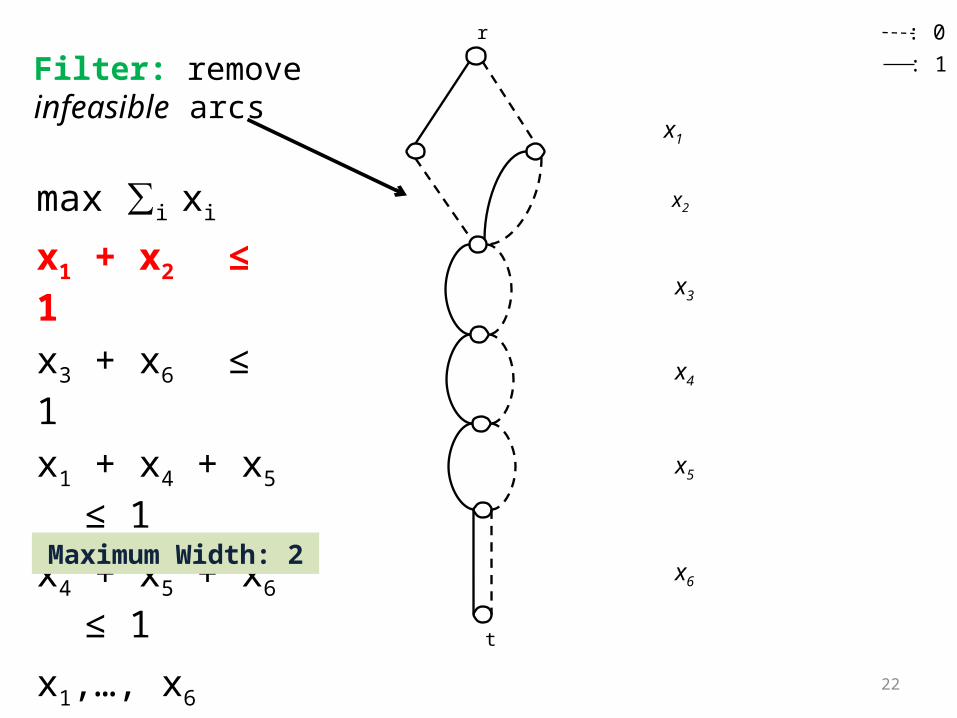
max ∑i xi
x1 + x2 ≤ 1
x3 + x6 ≤ 1
x1 + x4 + x5 ≤ 1
x4 + x5 + x6 ≤ 1
x1,…, x6 {0,1}
Filter: remove infeasible arcs
Maximum Width: 2
23
r
t
: 0: 1
x1
x2
x3
x4
x5
x6
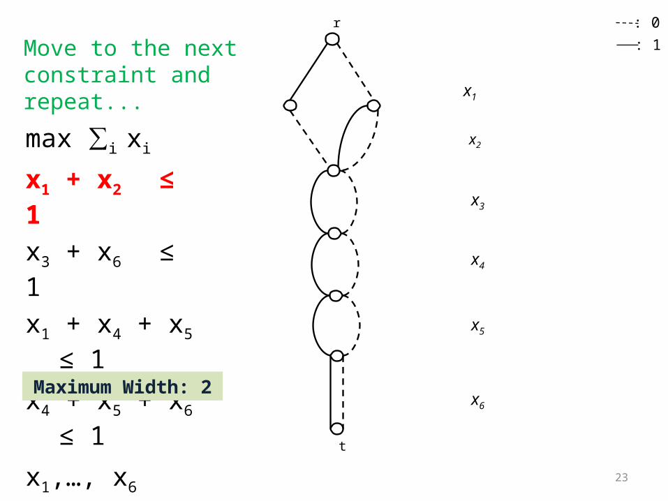
Move to the next constraint and repeat...
max ∑i xi
x1 + x2 ≤ 1
x3 + x6 ≤ 1
x1 + x4 + x5 ≤ 1
x4 + x5 + x6 ≤ 1
x1,…, x6 {0,1}
Maximum Width: 2
24
• Constraints can be highly-structured
• Suitable to scheduling
• Two application examples– Timetable problems– Disjunctive scheduling
Key Observation
25
Example:
• Allocate work days and rest days for an employee throughout the week
• Each employee must have at least one rest day for every three consecutive days – Sequence constraint
Timetable Problems
26
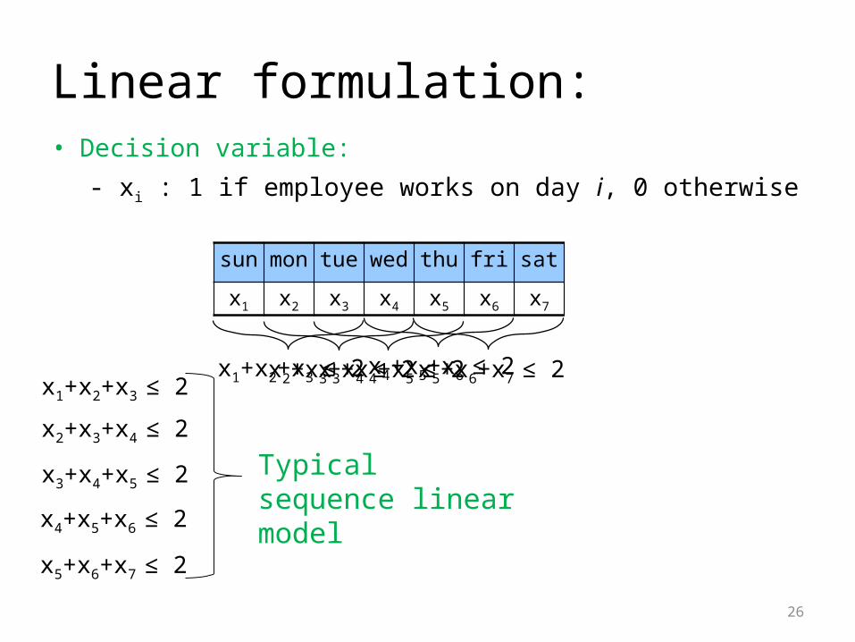
Linear formulation:
sun mon tue wed thu fri sat
x1 x2 x3 x4 x5 x6 x7
• Decision variable: - xi : 1 if employee works on day i, 0 otherwise
x2+x3+x4 ≤ 2x3+x4+x5 ≤ 2x4+x5+x6 ≤ 2x5+x6+x7 ≤ 2x1+x2+x3 ≤ 2x1+x2+x3 ≤ 2
x2+x3+x4 ≤ 2
x3+x4+x5 ≤ 2
x4+x5+x6 ≤ 2
x5+x6+x7 ≤ 2
Typical sequence linear model
27
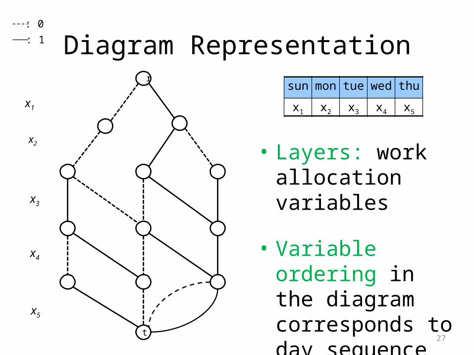
Diagram Representation
• Layers: work allocation variables
• Variable ordering in the diagram corresponds to day sequence
x1
x2
x3
x4
x5
r
t
: 0: 1
sun mon tue wed thu
x1 x2 x3 x4 x5
28
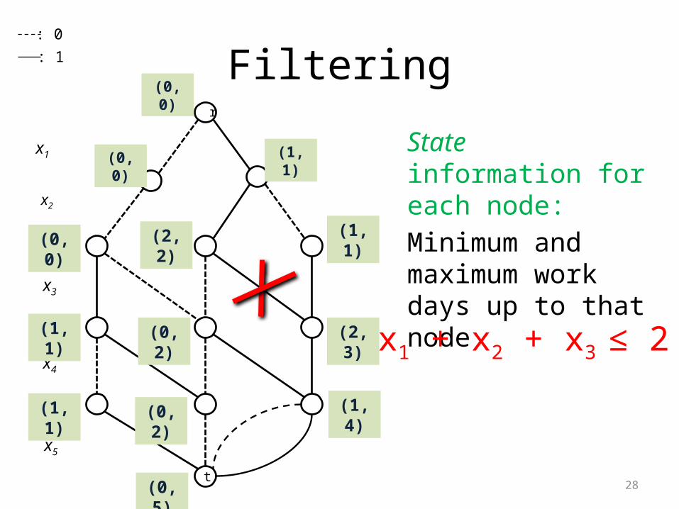
Filtering x1
x2
x3
x4
x5
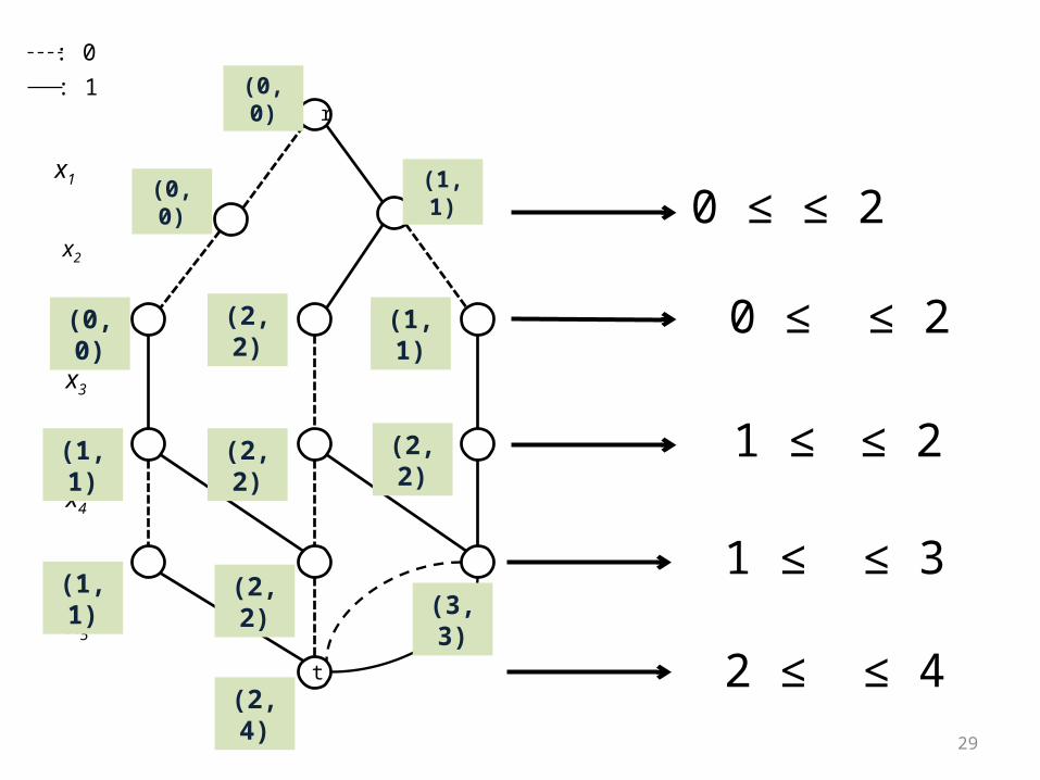
State information for each node: Minimum and maximum work days up to that node
x1 + x2 + x3 ≤ 2
(0, 0)
(0, 0) (1, 1)
(0, 0)
(1, 1)
(1, 1)
(2, 2)
(0, 2)
(1, 1)
(2, 3)
(1, 4)(0, 2)
(0, 5)
r
t
: 0: 1
29
x1
x2
x3
x4
x5
0 ≤ ≤ 2
0 ≤ ≤ 2
1 ≤ ≤ 2
1 ≤ ≤ 3
2 ≤ ≤ 4
(0, 0)
(0, 0) (1, 1)
(0, 0)
(1, 1)
(1, 1)
(2, 2)
(2, 2)
(1, 1)
(2, 2)
(3, 3)(2, 2)
(2, 4)
r
t
: 0: 1
30
• Hard randomly generated instances– 50 days– 5 sequence constraints
• Inference was incorporated into a state-of-the-art constraint-based scheduler (ILOG CP Optimizer)– New type of global constraint
Experimental Results
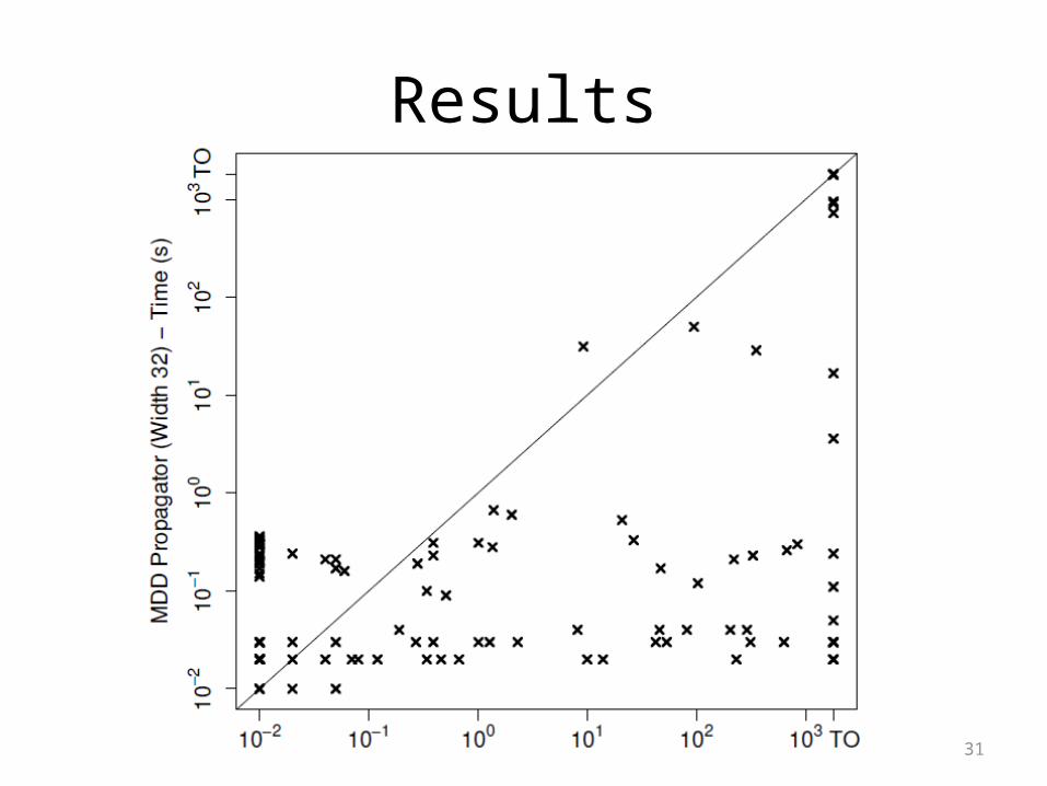
31
Results
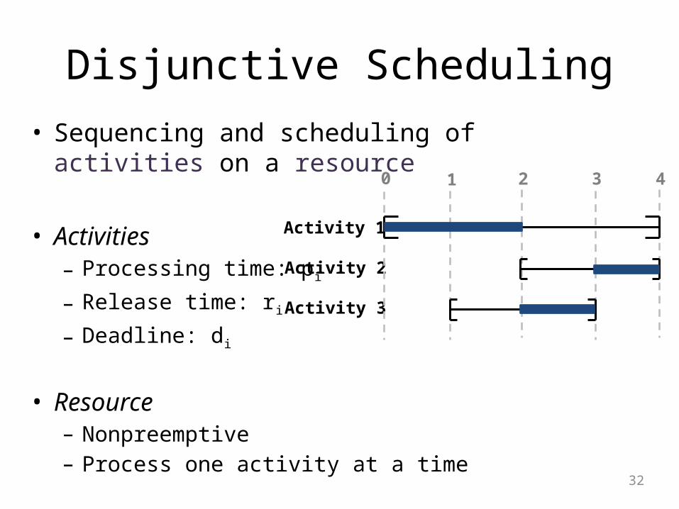
Disjunctive Scheduling• Sequencing and scheduling of activities on a resource
• Activities– Processing time: pi
– Release time: ri
– Deadline: di
• Resource– Nonpreemptive– Process one activity at a time
Activity 1
Activity 2
Activity 3
0 1 2 3 4
32
33
34
Diagram Representation
• Natural representation as permutation diagram
• Every solution can be written as a permutation π
π1, π2 , π3, …, πn : activity sequencing in the resource
• Schedule is implied by a sequence:
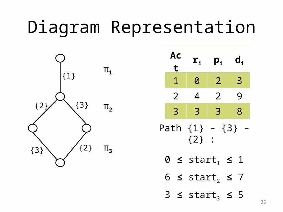
35
π1
π2
π3
{2}
{1}
{3}
{3} {2}
Path {1} – {3} – {2} :
0 ≤ start1 ≤ 1
6 ≤ start2 ≤ 7
3 ≤ start3 ≤ 5
Act ri pi di
1 0 2 3
2 4 2 9
3 3 3 8
Diagram Representation
36
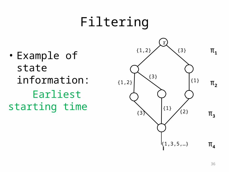
Filtering
• Example of state information:
Earliest starting time
π1
π2
π3
π4
r
{1,2}
{1,2}
{3}
{1}{3}
{3}{1}
{2}
{1,3,5,…}…
37
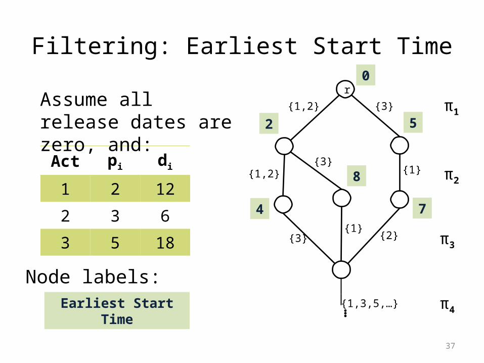
Filtering: Earliest Start Time
Act pi di
1 2 122 3 63 5 18
π1
π2
π3
π4
r
{1,2}
{1,2}
{3}
{1}{3}
{3}{1}
{2}
{1,3,5,…}…
Assume all release dates are zero, and:
0
2 5
74
8
Earliest Start Time
Node labels:
38
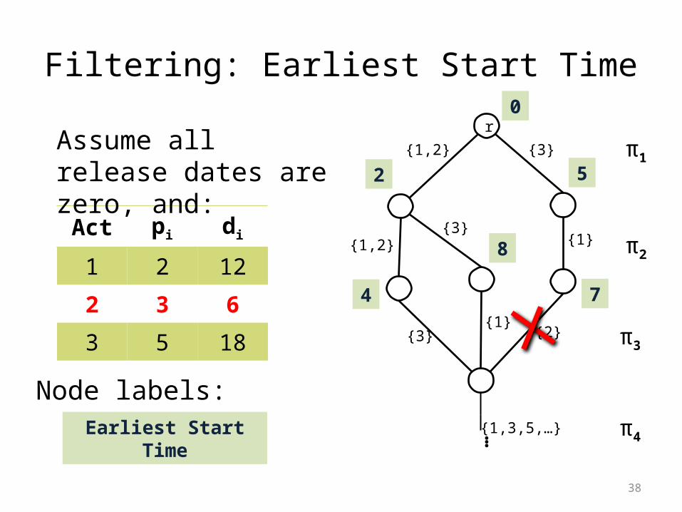
Filtering: Earliest Start Time
Act pi di
1 2 122 3 63 5 18
π1
π2
π3
π4
r
{1,2}
{1,2}
{3}
{1}{3}
{3}{1}
{2}
{1,3,5,…}…
Assume all release dates are zero, and:
0
2 5
74
8
Earliest Start Time
Node labels:
39
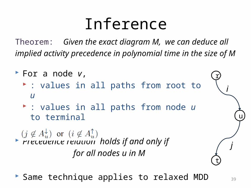
InferenceTheorem: Given the exact diagram M, we can deduce all implied activity precedence in polynomial time in the size of M
r
u
t
i
j
For a node v, : values in all paths from root to u : values in all paths from node u to terminal
Precedence relation holds if and only if for all nodes u in M
Same technique applies to relaxed MDD
40
Precedence relations can be used to:
• Guide search
• As an inference technique– Mathematical Programming: linear constraints– Constraint-based scheduling: reduce domains
Conversely, precedence relations can also be used to filter the permutation diagram
41
Experiments
• Decision diagram incorporated into IBM ILOG CPLEX CP Optimizer 12.4 (CPO)– State-of-the-art constraint based scheduling solver– Uses a portfolio of inference techniques and LP relaxation– Added as user-defined propagator
42
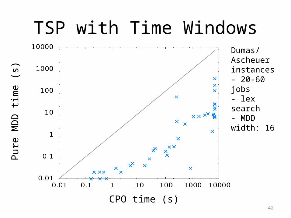
TSP with Time WindowsDumas/Ascheuer instances- 20-60 jobs- lex search- MDD width: 16
Pure
MD
D ti
me
(s)
CPO time (s)
43
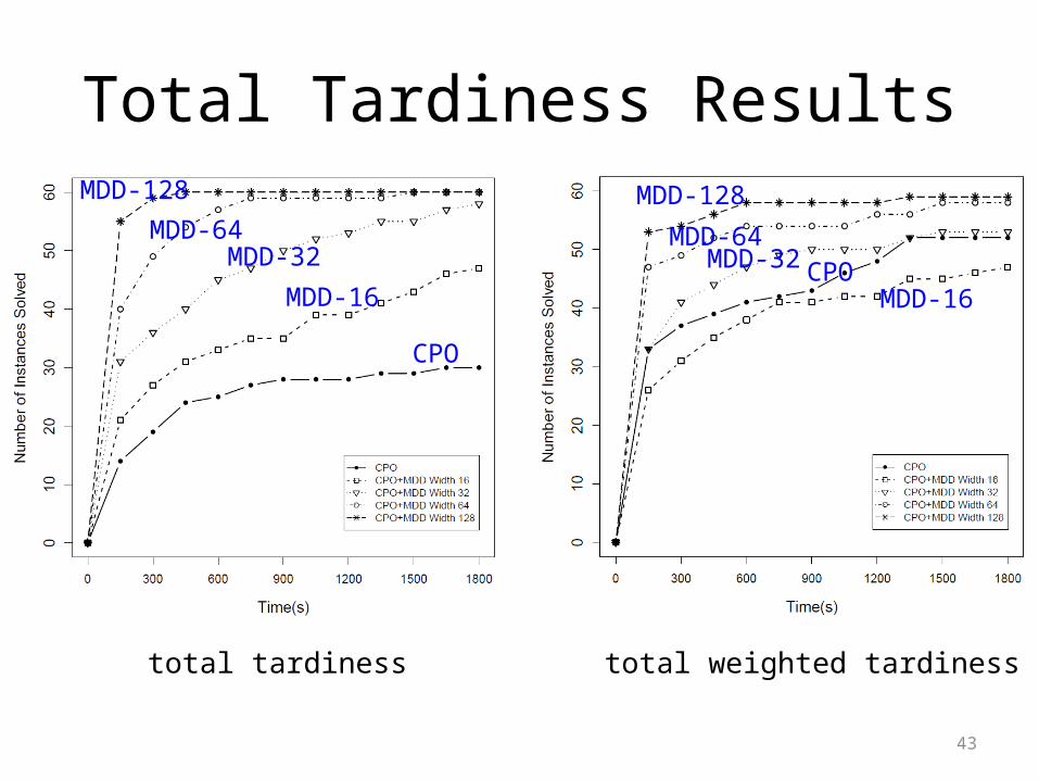
Total Tardiness Results
total tardiness total weighted tardiness
CPO
MDD-16
MDD-32MDD-64
MDD-128
CPOMDD-16
MDD-32MDD-64
MDD-128
44
Other results
• Asymmetric TSP with Precedence Constraints– Closed 3 open instances
• Similar results to more complex problems– Example: Machine deterioration
45
Final Remarks
• New approach for scheduling applications– Orders of magnitude speed-ups
• Bounding mechanism
• Provide highly-structured information that can be sent to existing solvers

Thank you!

47
Scheduling: Allocation of resources to tasks over time
• ≈ 60 years of research
• Still a fundamental component in supply chain management and optimization
48
Recent Franz Elderman Award Winners
• TNT Express, 2012– Network routing and scheduling
• Netherland Railways, 2008– Timetable
• Warner Robin Air Logistics, 2006– Allocation of repair tasks
• ...
49
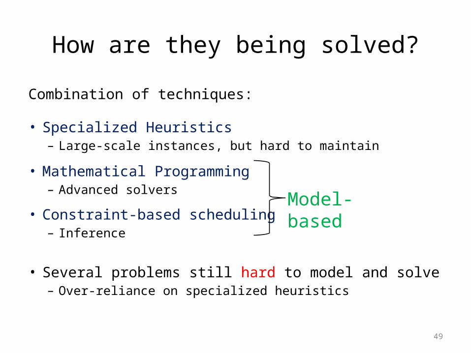
How are they being solved?
Combination of techniques:
• Specialized Heuristics– Large-scale instances, but hard to maintain
• Mathematical Programming– Advanced solvers
• Constraint-based scheduling– Inference
• Several problems still hard to model and solve– Over-reliance on specialized heuristics
Model-based
50
Scheduling: Allocation of resources to tasks over time
• ≈ 60 years of research
• Still a fundamental component in supply chain management and optimization
51
A new approach
Application of decision diagrams to scheduling
Quick highlights:– Modeling paradigm close to dynamic programming
– Technique can be incorporated into constraint-based schedulers, mathematical programming solvers, or heuristics
– Orders of magnitude speed-ups in several problem classes
52
Decision Diagrams for Optimization
Novel techniques for discrete optimization problems:
• C., van Hoeve: Multivalued Decision Diagrams for Sequencing Problems, Operations Research, to appear.
• Bergman, C., van Hoeve, Hooker: Optimization Bounds from Binary Decision Diagrams. INFORMS J. Computing, to appear.
• Bergman, C., van Hoeve, Hooker: Variable Ordering for the Application of BDDs to the Maximum Independent Set Problem. CPAIOR 2012: 34-49
• Bergman, C., van Hoeve, Yunes: BDD-Based Heuristics for Binary Optimization. Under review, 2013.
• Bergman, C., van Hoeve, Hooker: Decision Diagrams for Discrete Optimization. Under review, 2013.
• ...
Recommended