Data MiningCluster Analysis Basics
From Introduction to Data Mining by Tan, Steinbach, Kumar
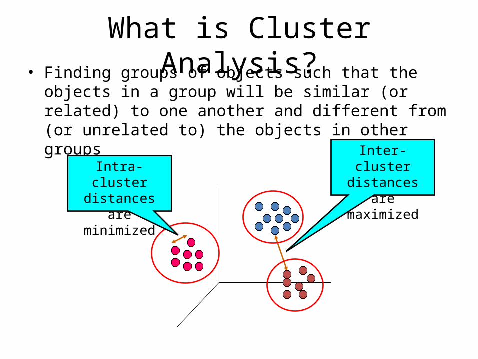
What is Cluster Analysis?• Finding groups of objects such that the objects in a group will
be similar (or related) to one another and different from (or unrelated to) the objects in other groups
Inter-cluster distances are maximized
Intra-cluster distances are
minimized

Applications of Cluster Analysis
• Understanding– Group related documents for
browsing, group genes and proteins that have similar functionality, or group stocks with similar price fluctuations
• Summarization– Reduce the size of large data
sets
Discovered Clusters Industry Group
1 Applied-Matl-DOWN,Bay-Network-Down,3-COM-DOWN,
Cabletron-Sys-DOWN,CISCO-DOWN,HP-DOWN, DSC-Comm-DOWN,INTEL-DOWN,LSI-Logic-DOWN,
Micron-Tech-DOWN,Texas-Inst-Down,Tellabs-Inc-Down, Natl-Semiconduct-DOWN,Oracl-DOWN,SGI-DOWN,
Sun-DOWN
Technology1-DOWN
2 Apple-Comp-DOWN,Autodesk-DOWN,DEC-DOWN,
ADV-Micro-Device-DOWN,Andrew-Corp-DOWN, Computer-Assoc-DOWN,Circuit-City-DOWN,
Compaq-DOWN, EMC-Corp-DOWN, Gen-Inst-DOWN, Motorola-DOWN,Microsoft-DOWN,Scientific-Atl-DOWN
Technology2-DOWN
3 Fannie-Mae-DOWN,Fed-Home-Loan-DOWN, MBNA-Corp-DOWN,Morgan-Stanley-DOWN
Financial-DOWN
4 Baker-Hughes-UP,Dresser-Inds-UP,Halliburton-HLD-UP,
Louisiana-Land-UP,Phillips-Petro-UP,Unocal-UP, Schlumberger-UP
Oil-UP
Clustering precipitation in Australia
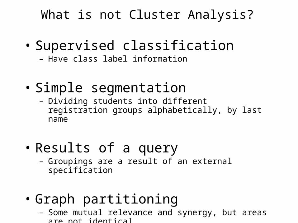
What is not Cluster Analysis?
• Supervised classification– Have class label information
• Simple segmentation– Dividing students into different registration groups alphabetically,
by last name
• Results of a query– Groupings are a result of an external specification
• Graph partitioning– Some mutual relevance and synergy, but areas are not identical

Notion of a Cluster can be Ambiguous
How many clusters?
Four Clusters Two Clusters
Six Clusters

Types of Clusterings
• A clustering is a set of clusters
• Important distinction between hierarchical and partitional sets of clusters
• Partitional Clustering– A division data objects into non-overlapping subsets (clusters) such
that each data object is in exactly one subset
• Hierarchical clustering– A set of nested clusters organized as a hierarchical tree

Partitional Clustering
Original Points A Partitional Clustering
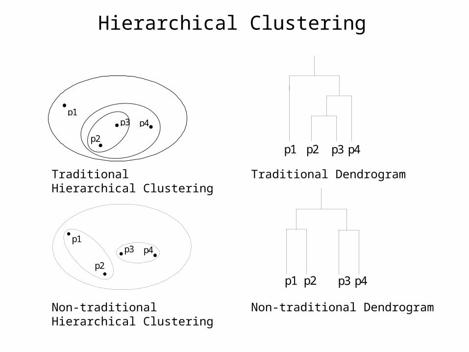
Hierarchical Clustering
p4p1
p3
p2
p4 p1
p3
p2
p4p1 p2 p3
p4p1 p2 p3
Traditional Hierarchical Clustering
Non-traditional Hierarchical Clustering
Non-traditional Dendrogram
Traditional Dendrogram

Other Distinctions Between Sets of Clusters
• Exclusive versus non-exclusive– In non-exclusive clusterings, points may belong to multiple clusters.– Can represent multiple classes or ‘border’ points
• Fuzzy versus non-fuzzy– In fuzzy clustering, a point belongs to every cluster with some
weight between 0 and 1– Weights must sum to 1– Probabilistic clustering has similar characteristics
• Partial versus complete– In some cases, we only want to cluster some of the data
• Heterogeneous versus homogeneous– Cluster of widely different sizes, shapes, and densities
Types of Clusters
• Well-separated clusters
• Center-based clusters
• Contiguous clusters
• Density-based clusters
• Property or Conceptual
• Described by an Objective Function
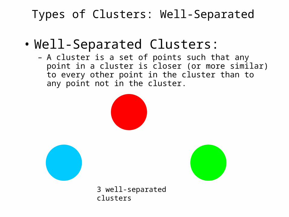
Types of Clusters: Well-Separated
• Well-Separated Clusters: – A cluster is a set of points such that any point in a cluster is closer
(or more similar) to every other point in the cluster than to any point not in the cluster.
3 well-separated clusters

Types of Clusters: Center-Based
• Center-based– A cluster is a set of objects such that an object in a cluster is closer
(more similar) to the “center” of a cluster, than to the center of any other cluster
– The center of a cluster is often a centroid, the average of all the points in the cluster, or a medoid, the most “representative” point of a cluster
4 center-based clusters

Types of Clusters: Contiguity-Based
• Contiguous Cluster (Nearest neighbor or Transitive)– A cluster is a set of points such that a point in a cluster is closer (or
more similar) to one or more other points in the cluster than to any point not in the cluster.
8 contiguous clusters
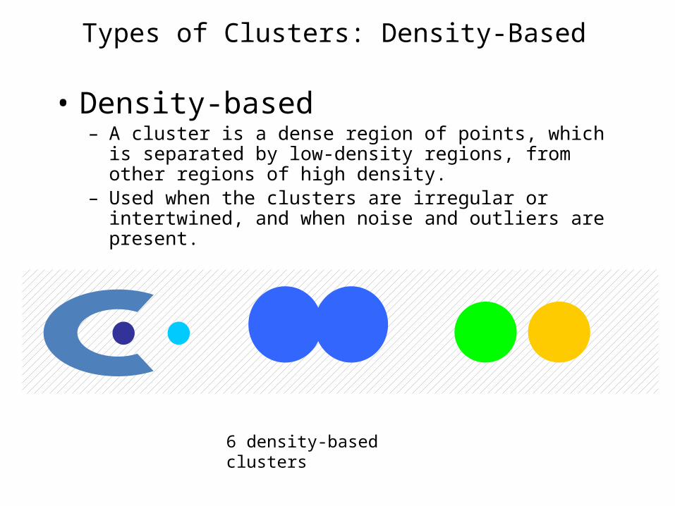
Types of Clusters: Density-Based
• Density-based– A cluster is a dense region of points, which is separated by low-
density regions, from other regions of high density. – Used when the clusters are irregular or intertwined, and when noise
and outliers are present.
6 density-based clusters
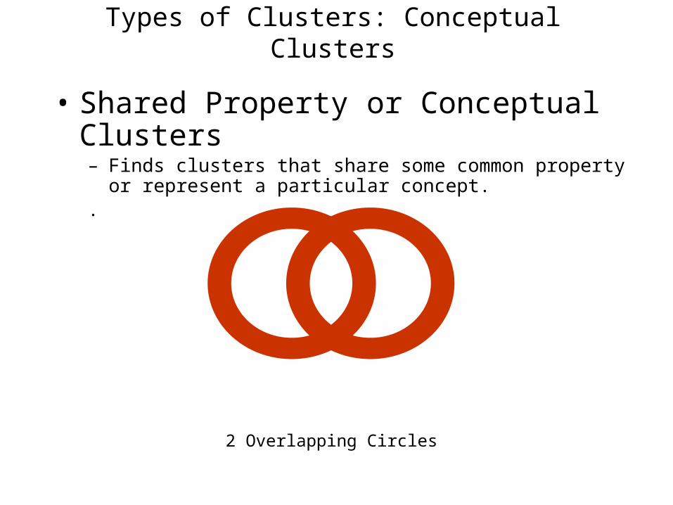
Types of Clusters: Conceptual Clusters
• Shared Property or Conceptual Clusters– Finds clusters that share some common property or represent a
particular concept. .
2 Overlapping Circles

Types of Clusters: Objective Function
• Clusters Defined by an Objective Function– Finds clusters that minimize or maximize an objective function. – Enumerate all possible ways of dividing the points into clusters and
evaluate the `goodness' of each potential set of clusters by using the given objective function. (NP Hard)
– Can have global or local objectives.• Hierarchical clustering algorithms typically have local objectives• Partitional algorithms typically have global objectives
– A variation of the global objective function approach is to fit the data to a parameterized model.
• Parameters for the model are determined from the data. • Mixture models assume that the data is a ‘mixture' of a number of statistical
distributions.

Types of Clusters: Objective Function …
• Map the clustering problem to a different domain and solve a related problem in that domain– Proximity matrix defines a weighted graph, where the
nodes are the points being clustered, and the weighted edges represent the proximities between points
– Clustering is equivalent to breaking the graph into connected components, one for each cluster.
– Want to minimize the edge weight between clusters and maximize the edge weight within clusters
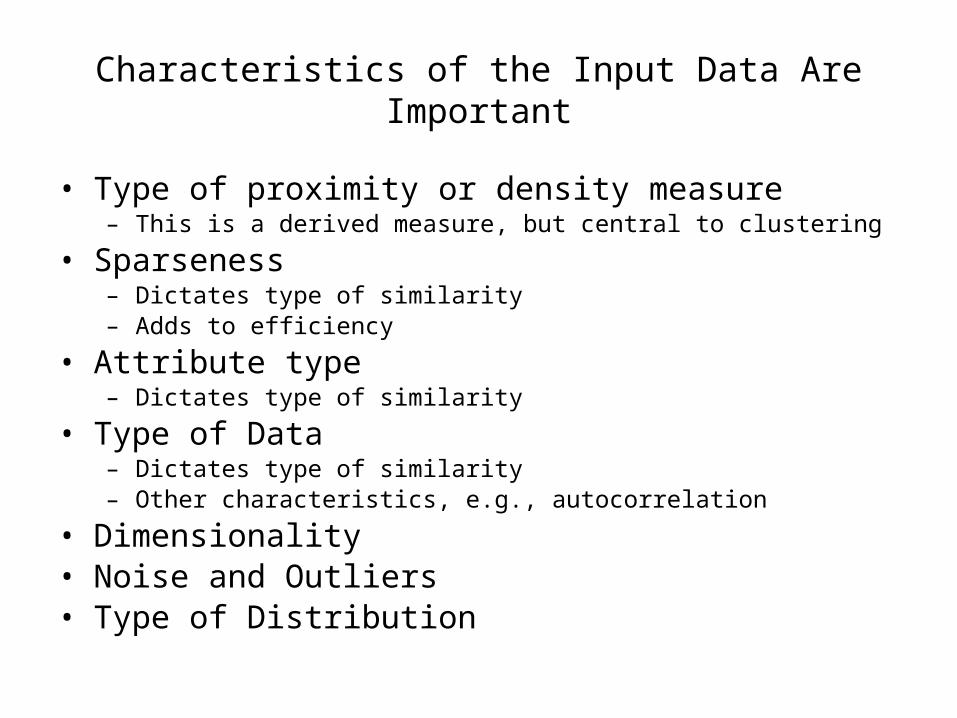
Characteristics of the Input Data Are Important
• Type of proximity or density measure– This is a derived measure, but central to clustering
• Sparseness– Dictates type of similarity– Adds to efficiency
• Attribute type– Dictates type of similarity
• Type of Data– Dictates type of similarity– Other characteristics, e.g., autocorrelation
• Dimensionality• Noise and Outliers• Type of Distribution
Clustering Algorithms
• K-means and its variants
• Hierarchical clustering
• Density-based clustering
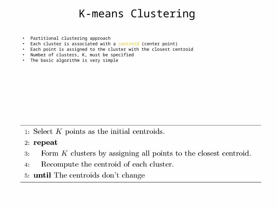
K-means Clustering
• Partitional clustering approach • Each cluster is associated with a centroid (center point) • Each point is assigned to the cluster with the closest centroid• Number of clusters, K, must be specified• The basic algorithm is very simple

K-means Clustering – Details• Initial centroids are often chosen randomly.
– Clusters produced vary from one run to another.• The centroid is (typically) the mean of the points in the cluster.• ‘Closeness’ is measured by Euclidean distance, cosine similarity, correlation, etc.• K-means will converge for common similarity measures mentioned above.• Most of the convergence happens in the first few iterations.
– Often the stopping condition is changed to ‘Until relatively few points change clusters’• Complexity is O( n * K * I * d )
– n = number of points, K = number of clusters, I = number of iterations, d = number of attributes

Two different K-means Clusterings
-2 -1.5 -1 -0.5 0 0.5 1 1.5 2
0
0.5
1
1.5
2
2.5
3
x
y
-2 -1.5 -1 -0.5 0 0.5 1 1.5 2
0
0.5
1
1.5
2
2.5
3
x
y
Sub-optimal Clustering
-2 -1.5 -1 -0.5 0 0.5 1 1.5 2
0
0.5
1
1.5
2
2.5
3
x
y
Optimal Clustering
Original Points
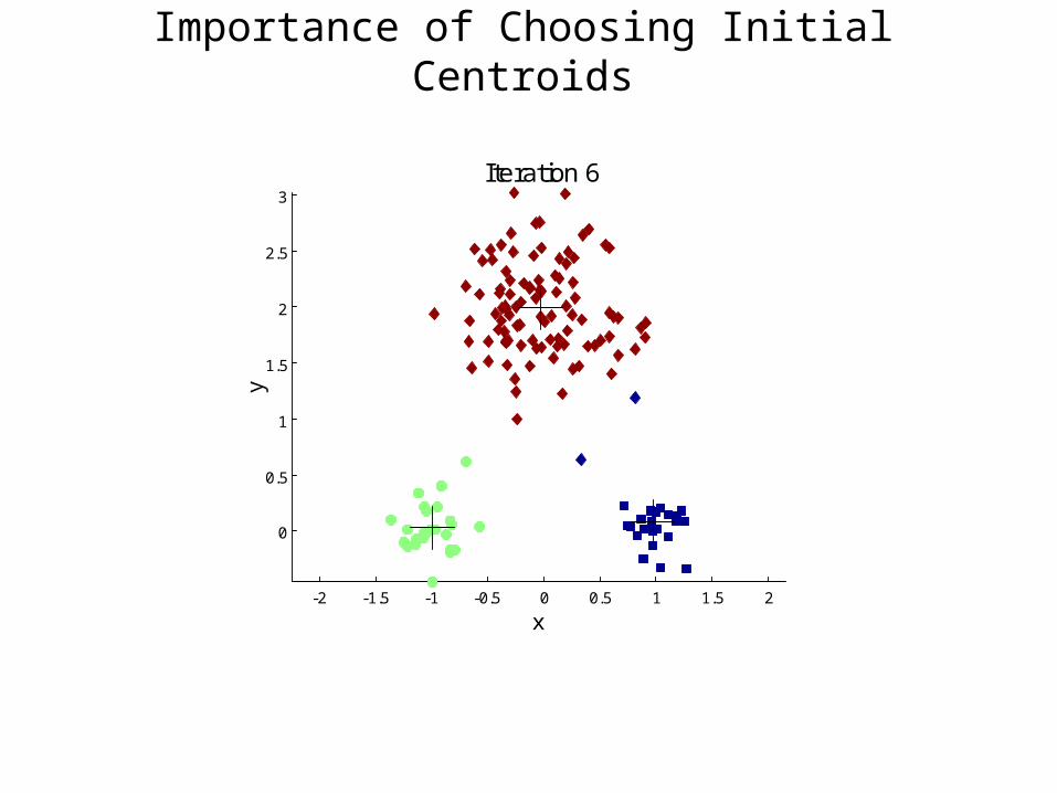
Importance of Choosing Initial Centroids
-2 -1.5 -1 -0.5 0 0.5 1 1.5 2
0
0.5
1
1.5
2
2.5
3
x
y
Iteration 1
-2 -1.5 -1 -0.5 0 0.5 1 1.5 2
0
0.5
1
1.5
2
2.5
3
x
y
Iteration 2
-2 -1.5 -1 -0.5 0 0.5 1 1.5 2
0
0.5
1
1.5
2
2.5
3
x
y
Iteration 3
-2 -1.5 -1 -0.5 0 0.5 1 1.5 2
0
0.5
1
1.5
2
2.5
3
x
y
Iteration 4
-2 -1.5 -1 -0.5 0 0.5 1 1.5 2
0
0.5
1
1.5
2
2.5
3
x
y
Iteration 5
-2 -1.5 -1 -0.5 0 0.5 1 1.5 2
0
0.5
1
1.5
2
2.5
3
x
y
Iteration 6
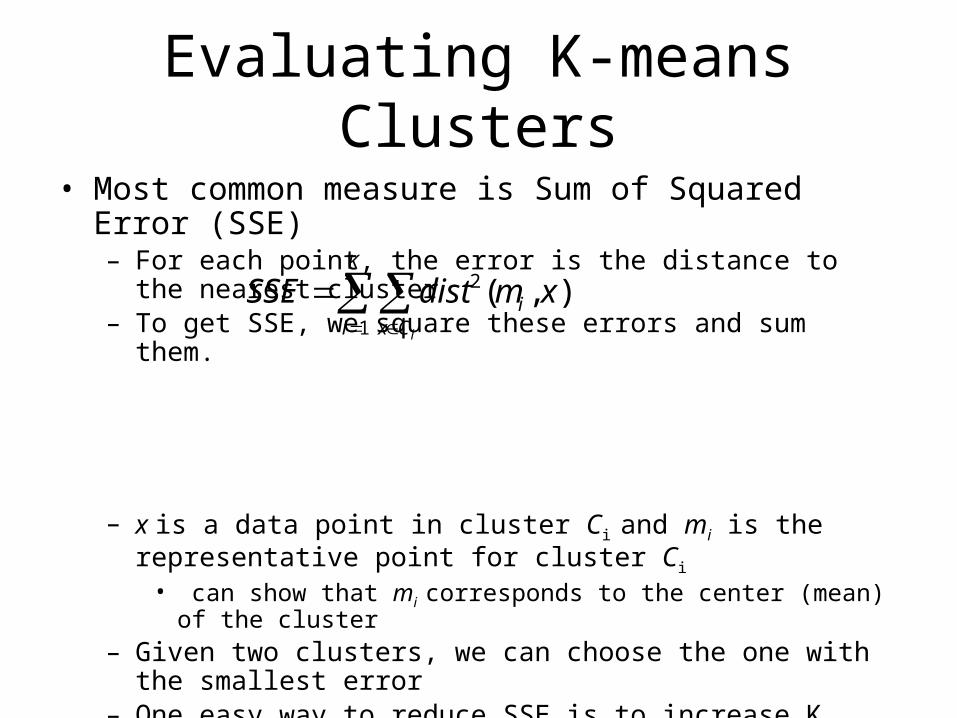
Evaluating K-means Clusters• Most common measure is Sum of Squared Error (SSE)
– For each point, the error is the distance to the nearest cluster– To get SSE, we square these errors and sum them.
– x is a data point in cluster Ci and mi is the representative point for cluster Ci
• can show that mi corresponds to the center (mean) of the cluster– Given two clusters, we can choose the one with the smallest error– One easy way to reduce SSE is to increase K, the number of clusters
• A good clustering with smaller K can have a lower SSE than a poor clustering with higher K
K
i Cxi
i
xmdistSSE1
2 ),(

Importance of Choosing Initial Centroids …
-2 -1.5 -1 -0.5 0 0.5 1 1.5 2
0
0.5
1
1.5
2
2.5
3
x
y
Iteration 1
-2 -1.5 -1 -0.5 0 0.5 1 1.5 2
0
0.5
1
1.5
2
2.5
3
x
y
Iteration 2
-2 -1.5 -1 -0.5 0 0.5 1 1.5 2
0
0.5
1
1.5
2
2.5
3
x
y
Iteration 3
-2 -1.5 -1 -0.5 0 0.5 1 1.5 2
0
0.5
1
1.5
2
2.5
3
x
y
Iteration 4
-2 -1.5 -1 -0.5 0 0.5 1 1.5 2
0
0.5
1
1.5
2
2.5
3
x
y
Iteration 5
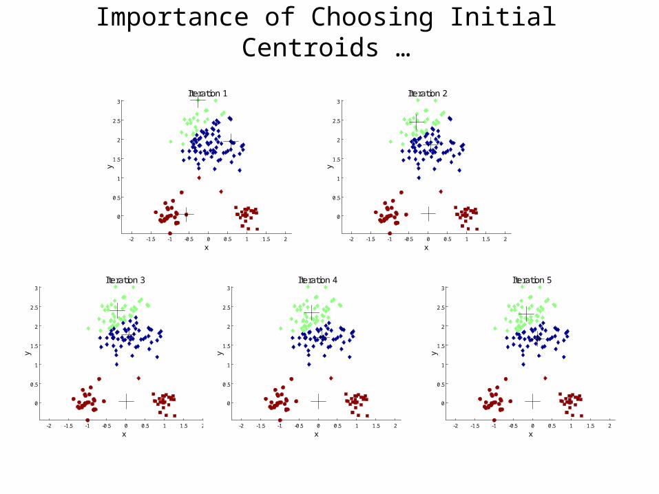
Importance of Choosing Initial Centroids …
-2 -1.5 -1 -0.5 0 0.5 1 1.5 2
0
0.5
1
1.5
2
2.5
3
x
y
Iteration 1
-2 -1.5 -1 -0.5 0 0.5 1 1.5 2
0
0.5
1
1.5
2
2.5
3
x
y
Iteration 2
-2 -1.5 -1 -0.5 0 0.5 1 1.5 2
0
0.5
1
1.5
2
2.5
3
x
y
Iteration 3
-2 -1.5 -1 -0.5 0 0.5 1 1.5 2
0
0.5
1
1.5
2
2.5
3
x
y
Iteration 4
-2 -1.5 -1 -0.5 0 0.5 1 1.5 2
0
0.5
1
1.5
2
2.5
3
xy
Iteration 5
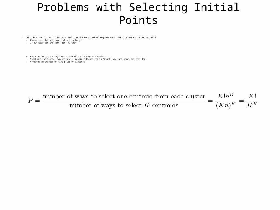
Problems with Selecting Initial Points
• If there are K ‘real’ clusters then the chance of selecting one centroid from each cluster is small. – Chance is relatively small when K is large– If clusters are the same size, n, then
– For example, if K = 10, then probability = 10!/1010 = 0.00036– Sometimes the initial centroids will readjust themselves in ‘right’ way, and sometimes they don’t– Consider an example of five pairs of clusters

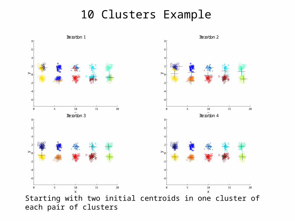
10 Clusters Example
0 5 10 15 20
-6
-4
-2
0
2
4
6
8
x
yIteration 1
0 5 10 15 20
-6
-4
-2
0
2
4
6
8
x
yIteration 2
0 5 10 15 20
-6
-4
-2
0
2
4
6
8
x
yIteration 3
0 5 10 15 20
-6
-4
-2
0
2
4
6
8
x
yIteration 4
Starting with two initial centroids in one cluster of each pair of clusters
10 Clusters Example
0 5 10 15 20
-6
-4
-2
0
2
4
6
8
x
y
Iteration 1
0 5 10 15 20
-6
-4
-2
0
2
4
6
8
x
y
Iteration 2
0 5 10 15 20
-6
-4
-2
0
2
4
6
8
x
y
Iteration 3
0 5 10 15 20
-6
-4
-2
0
2
4
6
8
x
y
Iteration 4
Starting with two initial centroids in one cluster of each pair of clusters

10 Clusters Example
Starting with some pairs of clusters having three initial centroids, while other have only one.
0 5 10 15 20
-6
-4
-2
0
2
4
6
8
x
y
Iteration 1
0 5 10 15 20
-6
-4
-2
0
2
4
6
8
x
y
Iteration 2
0 5 10 15 20
-6
-4
-2
0
2
4
6
8
x
y
Iteration 3
0 5 10 15 20
-6
-4
-2
0
2
4
6
8
x
y
Iteration 4

10 Clusters Example
Starting with some pairs of clusters having three initial centroids, while other have only one.
0 5 10 15 20
-6
-4
-2
0
2
4
6
8
x
yIteration 1
0 5 10 15 20
-6
-4
-2
0
2
4
6
8
x
y
Iteration 2
0 5 10 15 20
-6
-4
-2
0
2
4
6
8
x
y
Iteration 3
0 5 10 15 20
-6
-4
-2
0
2
4
6
8
x
y
Iteration 4
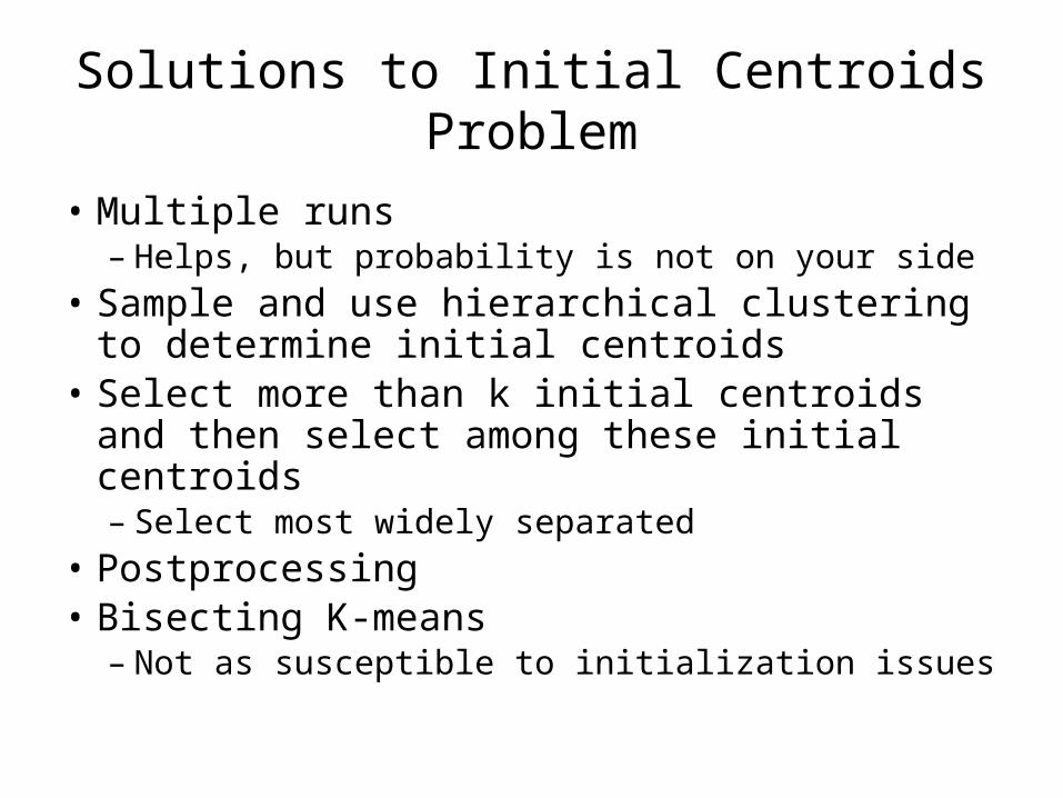
Solutions to Initial Centroids Problem
• Multiple runs– Helps, but probability is not on your side
• Sample and use hierarchical clustering to determine initial centroids
• Select more than k initial centroids and then select among these initial centroids– Select most widely separated
• Postprocessing• Bisecting K-means
– Not as susceptible to initialization issues
Handling Empty Clusters
• Basic K-means algorithm can yield empty clusters
• Several strategies– Choose the point that contributes most to SSE– Choose a point from the cluster with the highest
SSE– If there are several empty clusters, the above can
be repeated several times.

Updating Centers Incrementally
• In the basic K-means algorithm, centroids are updated after all points are assigned to a centroid
• An alternative is to update the centroids after each assignment (incremental approach)– Each assignment updates zero or two centroids– More expensive– Introduces an order dependency– Never get an empty cluster– Can use “weights” to change the impact

Pre-processing and Post-processing
• Pre-processing– Normalize the data– Eliminate outliers
• Post-processing– Eliminate small clusters that may represent outliers– Split ‘loose’ clusters, i.e., clusters with relatively high SSE– Merge clusters that are ‘close’ and that have relatively
low SSE– Can use these steps during the clustering process
• ISODATA
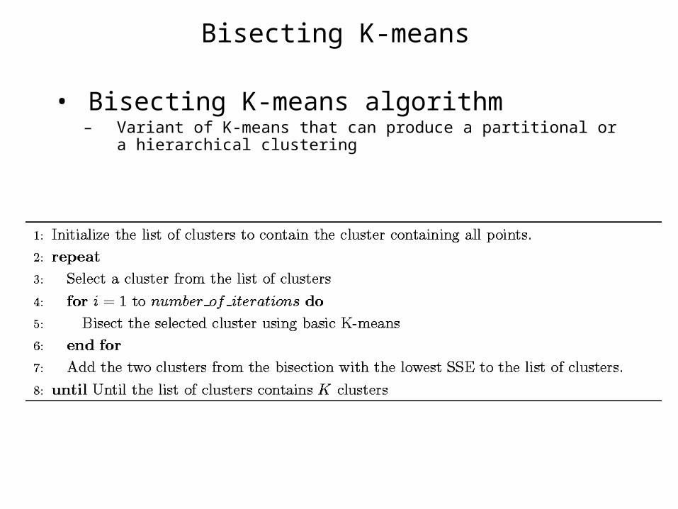
Bisecting K-means
• Bisecting K-means algorithm– Variant of K-means that can produce a partitional or a hierarchical
clustering

Bisecting K-means Example

Limitations of K-means
• K-means has problems when clusters are of differing – Sizes– Densities– Non-globular shapes
• K-means has problems when the data contains outliers.

Limitations of K-means: Differing Sizes
Original Points K-means (3 Clusters)
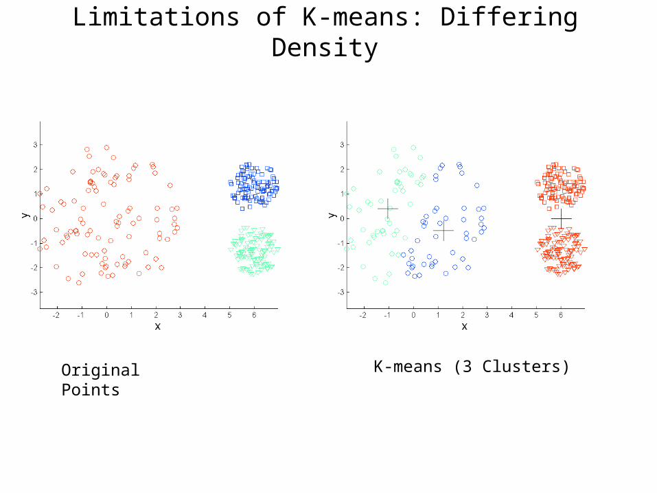
Limitations of K-means: Differing Density
Original Points K-means (3 Clusters)
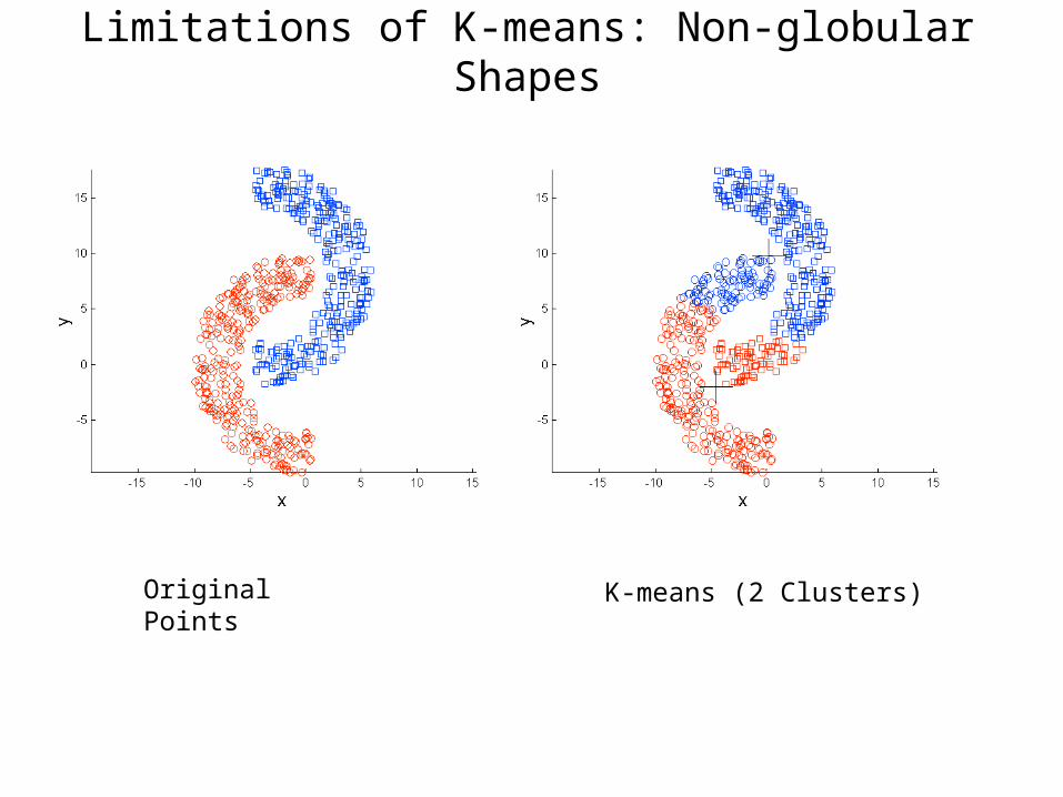
Limitations of K-means: Non-globular Shapes
Original Points K-means (2 Clusters)

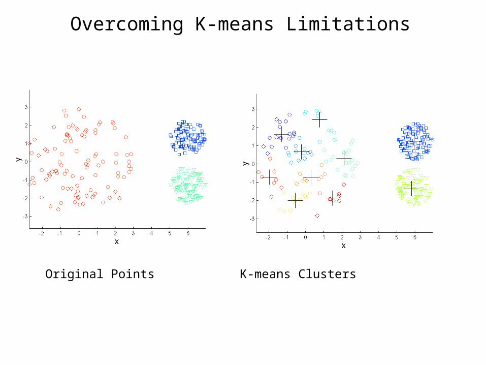
Overcoming K-means Limitations
Original Points K-means Clusters
One solution is to use many clusters.Find parts of clusters, but need to put together.
Overcoming K-means Limitations
Original Points K-means Clusters

Overcoming K-means Limitations
Original Points K-means Clusters

Hierarchical Clustering
• Produces a set of nested clusters organized as a hierarchical tree
• Can be visualized as a dendrogram– A tree like diagram that records the sequences of
merges or splits
1 3 2 5 4 60
0.05
0.1
0.15
0.2
1
2
3
4
5
6
1
23 4
5
Strengths of Hierarchical Clustering
• Do not have to assume any particular number of clusters– Any desired number of clusters can be obtained by
‘cutting’ the dendogram at the proper level
• They may correspond to meaningful taxonomies– Example in biological sciences (e.g., animal
kingdom, phylogeny reconstruction, …)
Hierarchical Clustering
• Two main types of hierarchical clustering– Agglomerative:
• Start with the points as individual clusters• At each step, merge the closest pair of clusters until only one cluster (or k
clusters) left
– Divisive: • Start with one, all-inclusive cluster • At each step, split a cluster until each cluster contains a point (or there are k
clusters)
• Traditional hierarchical algorithms use a similarity or distance matrix– Merge or split one cluster at a time

Agglomerative Clustering Algorithm
• More popular hierarchical clustering technique
• Basic algorithm is straightforward1. Compute the proximity matrix2. Let each data point be a cluster3. Repeat4. Merge the two closest clusters5. Update the proximity matrix6. Until only a single cluster remains
• Key operation is the computation of the proximity of two clusters
– Different approaches to defining the distance between clusters distinguish the different algorithms

Starting Situation
• Start with clusters of individual points and a proximity matrix p1
p3
p5p4
p2
p1 p2 p3 p4 p5 . . .
.
.
. Proximity Matrix
...p1 p2 p3 p4 p9 p10 p11 p12
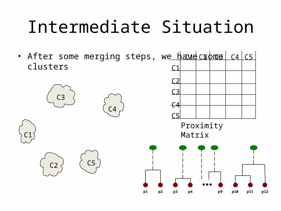
Intermediate Situation• After some merging steps, we have some clusters
C1
C4
C2 C5
C3
C2C1
C1
C3
C5
C4
C2
C3 C4 C5
Proximity Matrix
...p1 p2 p3 p4 p9 p10 p11 p12

Intermediate Situation• We want to merge the two closest clusters (C2 and C5) and update
the proximity matrix.
C1
C4
C2 C5
C3
C2C1
C1
C3
C5
C4
C2
C3 C4 C5
Proximity Matrix
...p1 p2 p3 p4 p9 p10 p11 p12
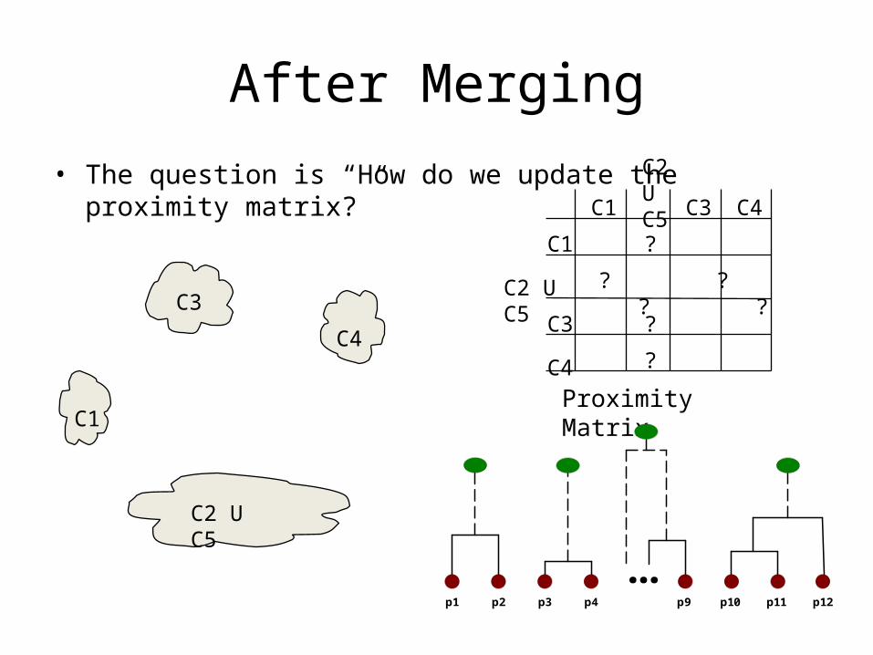
After Merging• The question is “How do we update the proximity matrix?”
C1
C4
C2 U C5
C3? ? ? ?
?
?
?
C2 U C5C1
C1
C3
C4
C2 U C5
C3 C4
Proximity Matrix
...p1 p2 p3 p4 p9 p10 p11 p12
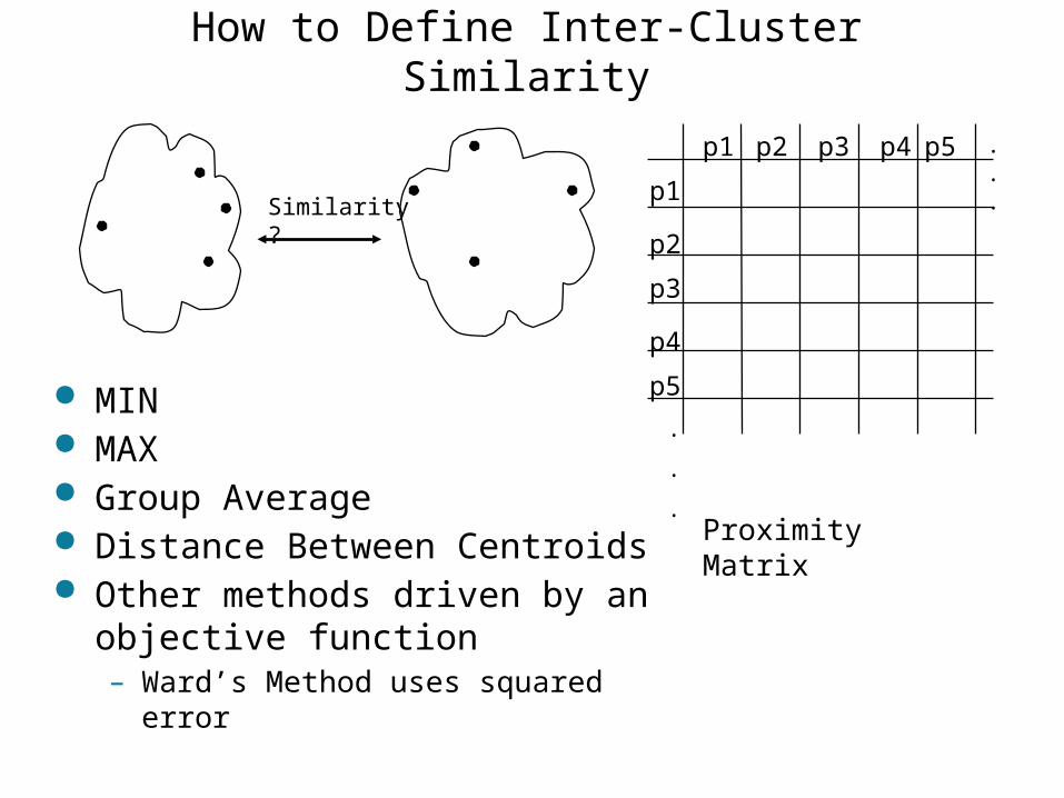
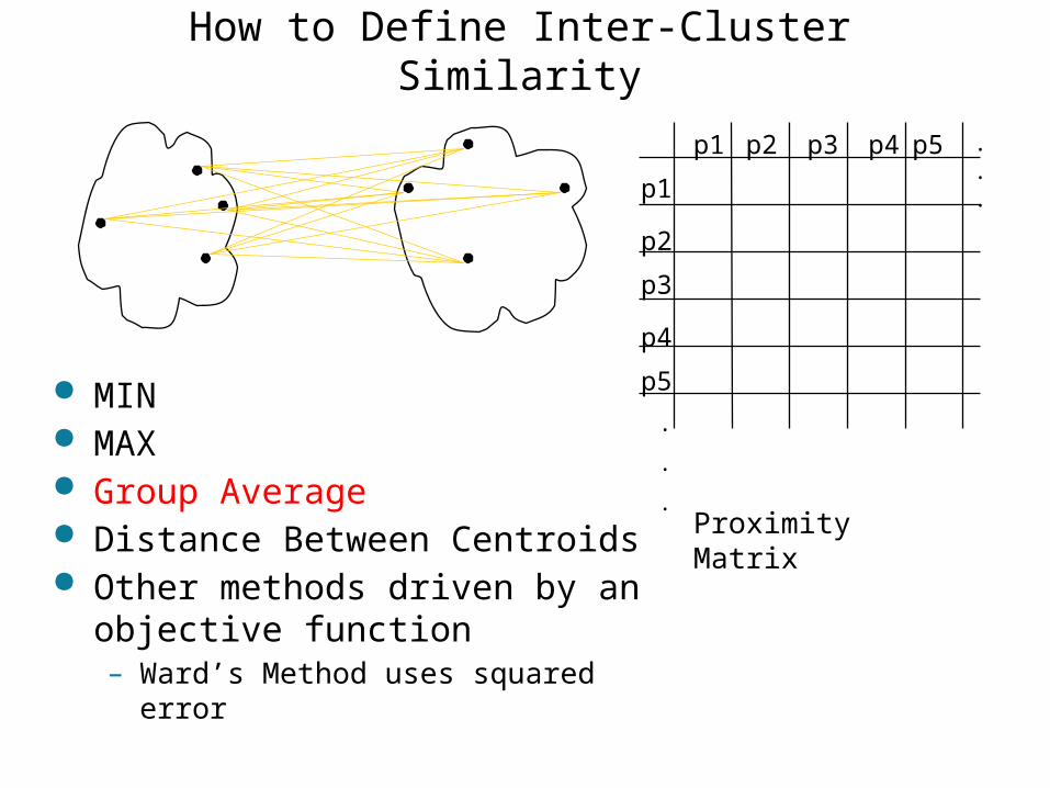
How to Define Inter-Cluster Similarity
p1
p3
p5
p4
p2
p1 p2 p3 p4 p5 . . .
.
.
.
Similarity?
MIN MAX Group Average Distance Between Centroids Other methods driven by an objective
function– Ward’s Method uses squared error
Proximity Matrix

How to Define Inter-Cluster Similarity
p1
p3
p5
p4
p2
p1 p2 p3 p4 p5 . . .
.
.
.Proximity Matrix
MIN MAX Group Average Distance Between Centroids Other methods driven by an objective
function– Ward’s Method uses squared error
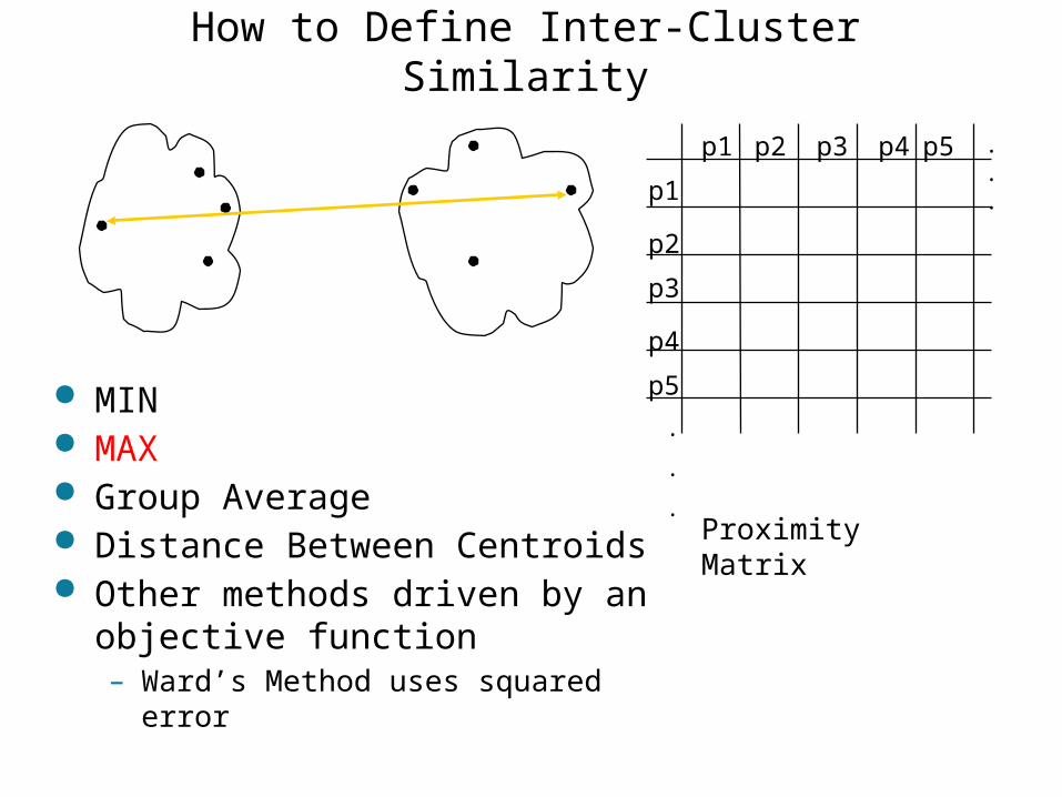
How to Define Inter-Cluster Similarity
p1
p3
p5
p4
p2
p1 p2 p3 p4 p5 . . .
.
.
.Proximity Matrix
MIN MAX Group Average Distance Between Centroids Other methods driven by an objective
function– Ward’s Method uses squared error
How to Define Inter-Cluster Similarity
p1
p3
p5
p4
p2
p1 p2 p3 p4 p5 . . .
.
.
.Proximity Matrix
MIN MAX Group Average Distance Between Centroids Other methods driven by an objective
function– Ward’s Method uses squared error

How to Define Inter-Cluster Similarity
p1
p3
p5
p4
p2
p1 p2 p3 p4 p5 . . .
.
.
.Proximity Matrix
MIN MAX Group Average Distance Between Centroids Other methods driven by an objective
function– Ward’s Method uses squared error

Cluster Similarity: MIN or Single Link
• Similarity of two clusters is based on the two most similar (closest) points in the different clusters– Determined by one pair of points, i.e., by one link
in the proximity graph.I1 I2 I3 I4 I5
I1 1.00 0.90 0.10 0.65 0.20I2 0.90 1.00 0.70 0.60 0.50I3 0.10 0.70 1.00 0.40 0.30I4 0.65 0.60 0.40 1.00 0.80I5 0.20 0.50 0.30 0.80 1.00 1 2 3 4 5

Hierarchical Clustering: MIN
Nested Clusters Dendrogram
1
2
3
4
5
6
12
3
4
5
3 6 2 5 4 10
0.05
0.1
0.15
0.2
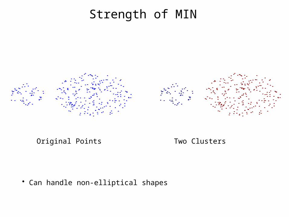
Strength of MIN
Original Points Two Clusters
• Can handle non-elliptical shapes
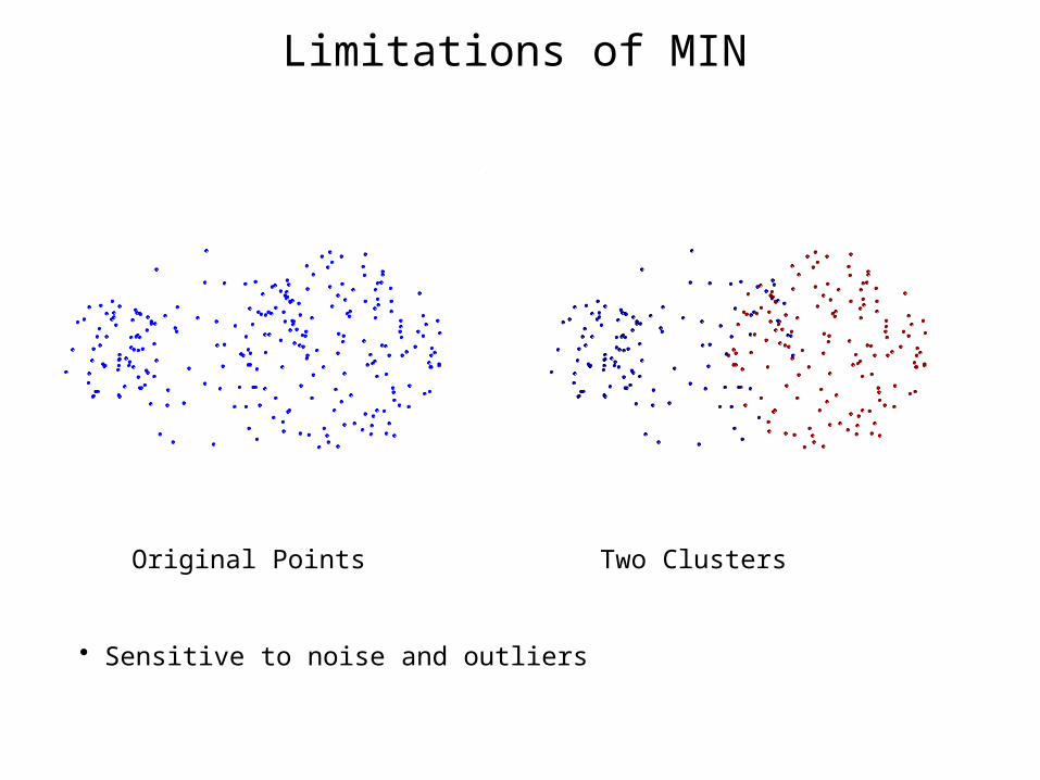
Limitations of MIN
Original Points Two Clusters
• Sensitive to noise and outliers

Cluster Similarity: MAX or Complete Linkage
• Similarity of two clusters is based on the two least similar (most distant) points in the different clusters– Determined by all pairs of points in the two
clustersI1 I2 I3 I4 I5I1 1.00 0.90 0.10 0.65 0.20I2 0.90 1.00 0.70 0.60 0.50I3 0.10 0.70 1.00 0.40 0.30I4 0.65 0.60 0.40 1.00 0.80I5 0.20 0.50 0.30 0.80 1.00 1 2 3 4 5
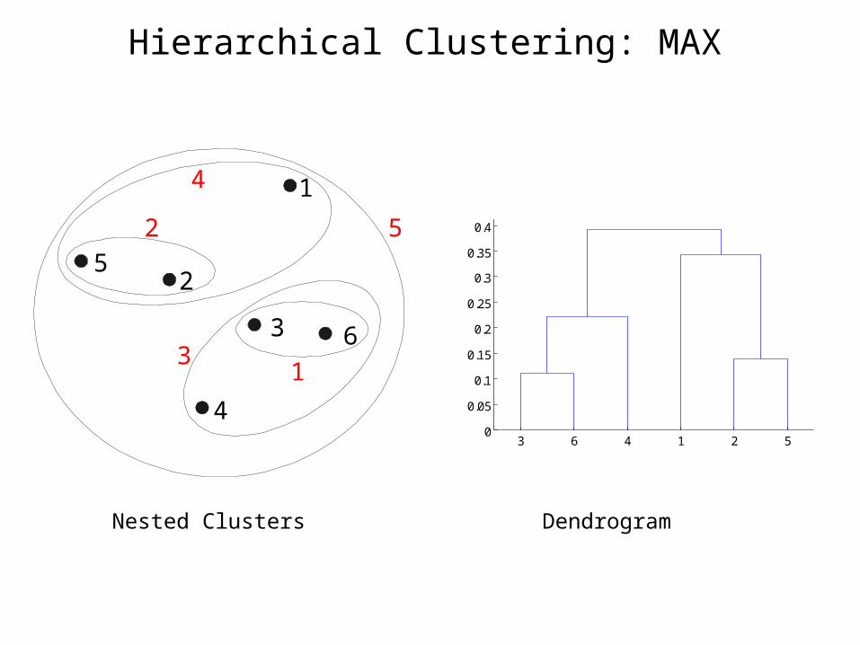
Hierarchical Clustering: MAX
Nested Clusters Dendrogram
3 6 4 1 2 50
0.05
0.1
0.15
0.2
0.25
0.3
0.35
0.4
1
2
3
4
5
6
1
2 5
3
4
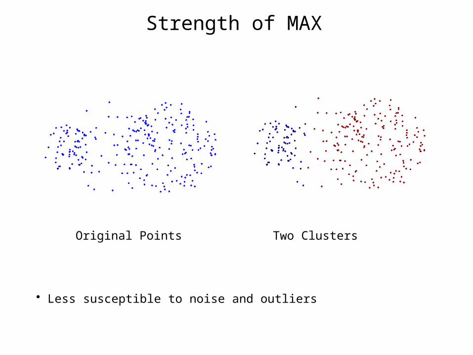
Strength of MAX
Original Points Two Clusters
• Less susceptible to noise and outliers
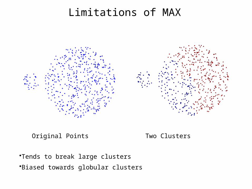
Limitations of MAX
Original Points Two Clusters
•Tends to break large clusters
•Biased towards globular clusters
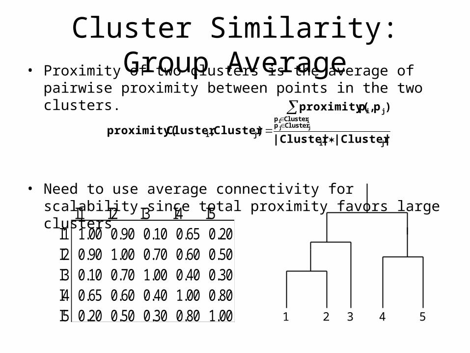
Cluster Similarity: Group Average• Proximity of two clusters is the average of pairwise proximity
between points in the two clusters.
• Need to use average connectivity for scalability since total proximity favors large clusters
||Cluster||Cluster
)p,pproximity(
)Cluster,Clusterproximity(ji
ClusterpClusterp
ji
jijjii
I1 I2 I3 I4 I5I1 1.00 0.90 0.10 0.65 0.20I2 0.90 1.00 0.70 0.60 0.50I3 0.10 0.70 1.00 0.40 0.30I4 0.65 0.60 0.40 1.00 0.80I5 0.20 0.50 0.30 0.80 1.00 1 2 3 4 5

Hierarchical Clustering: Group Average
Nested Clusters Dendrogram
3 6 4 1 2 50
0.05
0.1
0.15
0.2
0.25
1
2
3
4
5
6
1
2
5
3
4
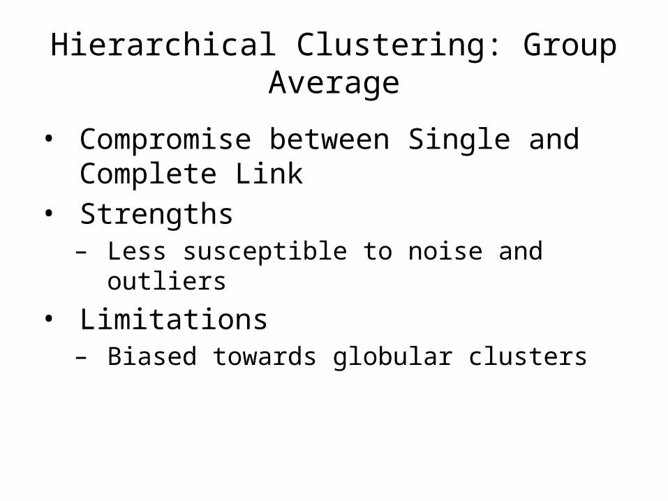
Hierarchical Clustering: Group Average
• Compromise between Single and Complete Link
• Strengths– Less susceptible to noise and outliers
• Limitations– Biased towards globular clusters

Cluster Similarity: Ward’s Method
• Similarity of two clusters is based on the increase in squared error when two clusters are merged– Similar to group average if distance between points is
distance squared
• Less susceptible to noise and outliers
• Biased towards globular clusters
• Hierarchical analogue of K-means– Can be used to initialize K-means

Hierarchical Clustering: Time and Space requirements
• O(N2) space since it uses the proximity matrix. – N is the number of points.
• O(N3) time in many cases– There are N steps and at each step the size, N2,
proximity matrix must be updated and searched– Complexity can be reduced to O(N2 log(N) ) time
for some approaches

Hierarchical Clustering: Problems and Limitations
• Once a decision is made to combine two clusters, it cannot be undone
• No objective function is directly minimized
• Different schemes have problems with one or more of the following:– Sensitivity to noise and outliers– Difficulty handling different sized clusters and convex
shapes– Breaking large clusters

Cluster Validity • For supervised classification we have a variety of measures to
evaluate how good our model is– Accuracy, precision, recall
• For cluster analysis, the analogous question is how to evaluate the “goodness” of the resulting clusters?
• But “clusters are in the eye of the beholder”!
• Then why do we want to evaluate them?– To avoid finding patterns in noise– To compare clustering algorithms– To compare two sets of clusters– To compare two clusters

Clusters found in Random Data
0 0.2 0.4 0.6 0.8 10
0.1
0.2
0.3
0.4
0.5
0.6
0.7
0.8
0.9
1
x
y
Random Points
0 0.2 0.4 0.6 0.8 10
0.1
0.2
0.3
0.4
0.5
0.6
0.7
0.8
0.9
1
x
y
K-means
0 0.2 0.4 0.6 0.8 10
0.1
0.2
0.3
0.4
0.5
0.6
0.7
0.8
0.9
1
x
y
DBSCAN
0 0.2 0.4 0.6 0.8 10
0.1
0.2
0.3
0.4
0.5
0.6
0.7
0.8
0.9
1
x
y
Complete Link
1. Determining the clustering tendency of a set of data, i.e., distinguishing whether non-random structure actually exists in the data.
2. Comparing the results of a cluster analysis to externally known results, e.g., to externally given class labels.
3. Evaluating how well the results of a cluster analysis fit the data without reference to external information.
- Use only the data
4. Comparing the results of two different sets of cluster analyses to determine which is better.
5. Determining the ‘correct’ number of clusters.
For 2, 3, and 4, we can further distinguish whether we want to evaluate the entire clustering or just individual clusters.
Different Aspects of Cluster Validation

• Numerical measures that are applied to judge various aspects of cluster validity, are classified into the following three types.– External Index: Used to measure the extent to which cluster labels match
externally supplied class labels.• Entropy
– Internal Index: Used to measure the goodness of a clustering structure without respect to external information.
• Sum of Squared Error (SSE)
– Relative Index: Used to compare two different clusterings or clusters. • Often an external or internal index is used for this function, e.g., SSE or entropy
• Sometimes these are referred to as criteria instead of indices– However, sometimes criterion is the general strategy and index is the numerical
measure that implements the criterion.
Measures of Cluster Validity

• Two matrices – Proximity Matrix– “Incidence” Matrix
• One row and one column for each data point• An entry is 1 if the associated pair of points belong to the same cluster• An entry is 0 if the associated pair of points belongs to different clusters
• Compute the correlation between the two matrices– Since the matrices are symmetric, only the correlation between
n(n-1) / 2 entries needs to be calculated.
• High correlation indicates that points that belong to the same cluster are close to each other.
• Not a good measure for some density or contiguity based clusters.
Measuring Cluster Validity Via Correlation

Measuring Cluster Validity Via Correlation• Correlation of incidence and proximity matrices for the K-means clusterings of the following two data sets.
• Order the similarity matrix with respect to cluster labels and inspect visually.
0 0.2 0.4 0.6 0.8 10
0.1
0.2
0.3
0.4
0.5
0.6
0.7
0.8
0.9
1
x
y
0 0.2 0.4 0.6 0.8 10
0.1
0.2
0.3
0.4
0.5
0.6
0.7
0.8
0.9
1
x
yCorr = -0.9235
Corr = -0.5810
Points
Po
ints
20 40 60 80 100
10
20
30
40
50
60
70
80
90
100Similarity
0
0.1
0.2
0.3
0.4
0.5
0.6
0.7
0.8
0.9
1
Points
Po
ints
20 40 60 80 100
10
20
30
40
50
60
70
80
90
100Similarity
0
0.1
0.2
0.3
0.4
0.5
0.6
0.7
0.8
0.9
1
Clusters in random data are not so crisp
Recommended