Computational Biology Lecture Slides Week 10 Classification (some parts taken from Introduction to Data Mining by Tan, Steinbach, Kumar)

Computational Biology

Lecture Slides Week 10

Classification(some parts taken from

Introduction to Data Miningby

Tan, Steinbach, Kumar)

MBG404 Overview

Data

Generation

Processing

Storage

Mining

Pipelining

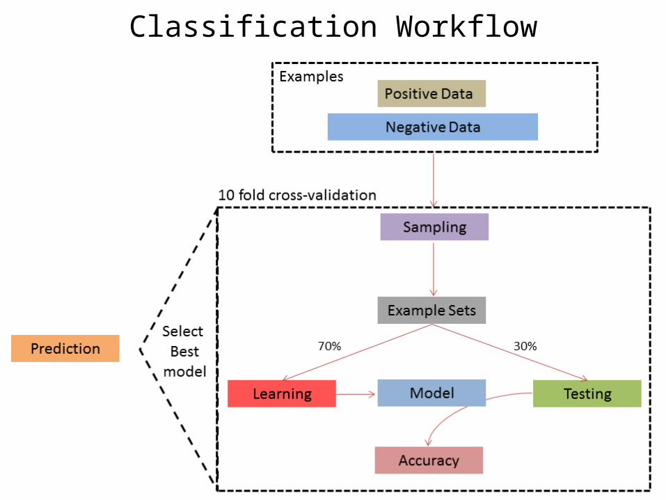
Classification Workflow

Support Vector Machines

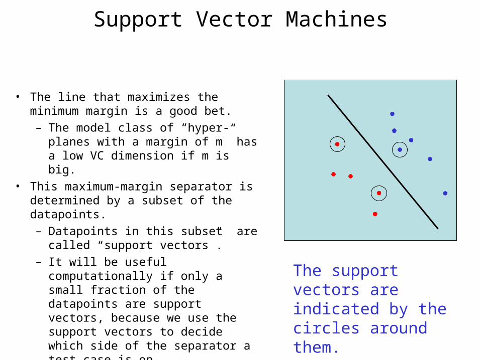
• The line that maximizes the minimum margin is a good bet.– The model class of “hyper-planes

with a margin of m” has a low VC dimension if m is big.

• This maximum-margin separator is determined by a subset of the datapoints.– Datapoints in this subset are

called “support vectors”.– It will be useful computationally if

only a small fraction of the datapoints are support vectors, because we use the support vectors to decide which side of the separator a test case is on.

The support vectors are indicated by the circles around them.

Training a linear SVM

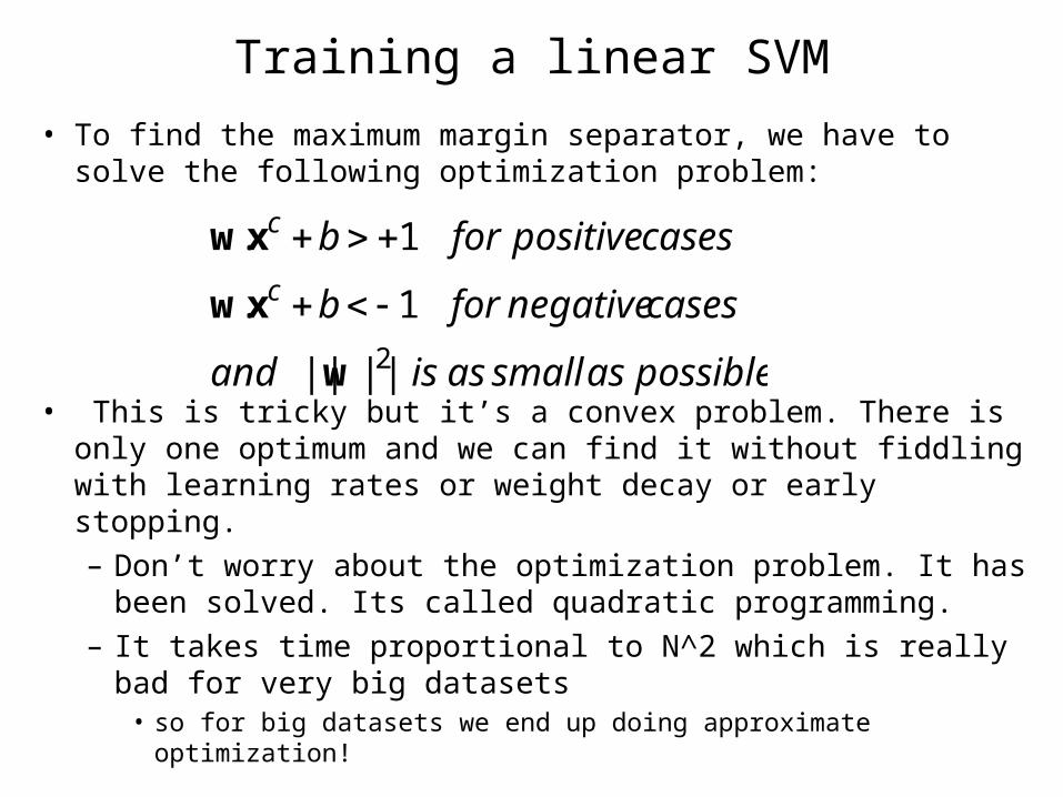
• To find the maximum margin separator, we have to solve the following optimization problem:

• This is tricky but it’s a convex problem. There is only one optimum and we can find it without fiddling with learning rates or weight decay or early stopping.– Don’t worry about the optimization problem. It has been

solved. Its called quadratic programming.– It takes time proportional to N^2 which is really bad for

very big datasets• so for big datasets we end up doing approximate optimization!

possibleassmallasisand

casesnegativeforb

casespositiveforbc

c

2||||

1.

1.

w

xw

xw

Testing a linear SVM

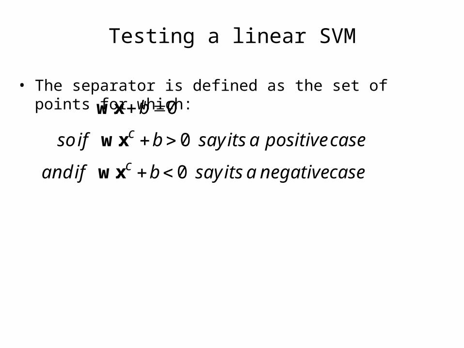
• The separator is defined as the set of points for which:

casenegativeaitssaybifand

casepositiveaitssaybifso

b

c

c

0.

0.

0.

xw

xw

xw

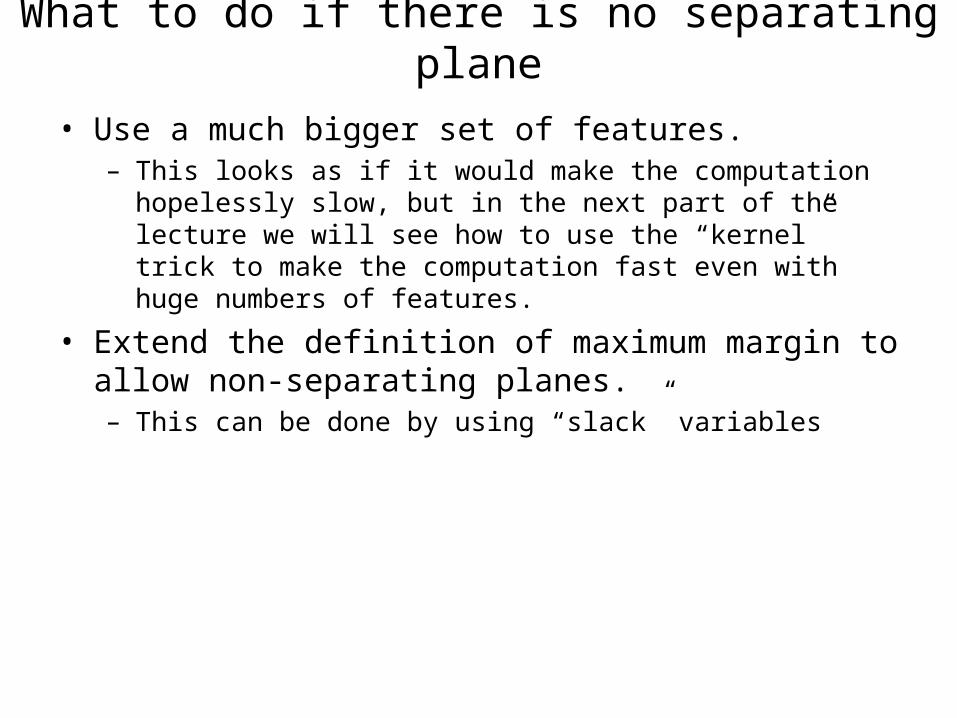
What to do if there is no separating plane

• Use a much bigger set of features.– This looks as if it would make the computation hopelessly slow,

but in the next part of the lecture we will see how to use the “kernel” trick to make the computation fast even with huge numbers of features.

• Extend the definition of maximum margin to allow non-separating planes.– This can be done by using “slack” variables

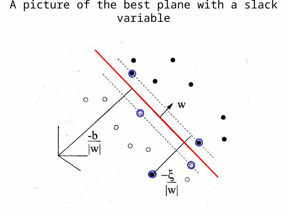
A picture of the best plane with a slack variable

The story so far

• If we use a large set of non-adaptive features, we can often make the two classes linearly separable.– But if we just fit any old separating plane, it will not

generalize well to new cases.• If we fit the separating plane that maximizes the margin

(the minimum distance to any of the data points), we will get much better generalization.– Intuitively, by maximizing the margin we are

squeezing out all the surplus capacity that came from using a high-dimensional feature space.

• This can be justified by a whole lot of clever mathematics which shows that– large margin separators have lower VC dimension.– models with lower VC dimension have a smaller gap

between the training and test error rates.

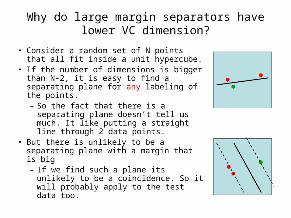
Why do large margin separators have lower VC dimension?

• Consider a random set of N points that all fit inside a unit hypercube.

• If the number of dimensions is bigger than N-2, it is easy to find a separating plane for any labeling of the points.– So the fact that there is a separating

plane doesn’t tell us much. It like putting a straight line through 2 data points.

• But there is unlikely to be a separating plane with a margin that is big– If we find such a plane its unlikely to

be a coincidence. So it will probably apply to the test data too.

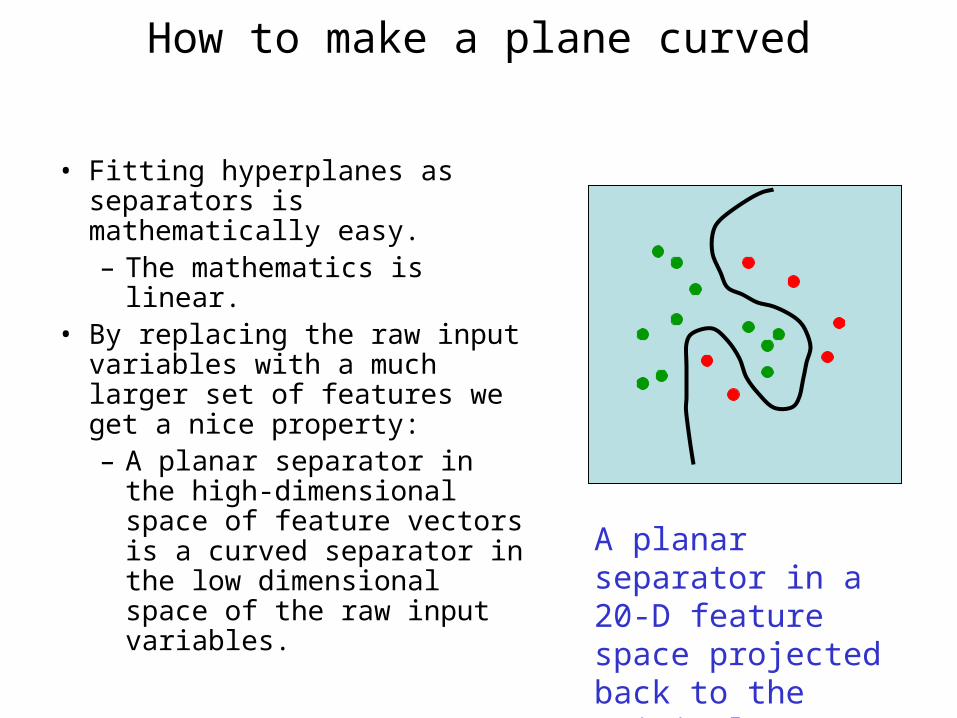
How to make a plane curved

• Fitting hyperplanes as separators is mathematically easy.– The mathematics is linear.

• By replacing the raw input variables with a much larger set of features we get a nice property:– A planar separator in the

high-dimensional space of feature vectors is a curved separator in the low dimensional space of the raw input variables.

A planar separator in a 20-D feature space projected back to the original 2-D space

A potential problem and a magic solution

• If we map the input vectors into a very high-dimensional feature space, surely the task of finding the maximum-margin separator becomes computationally intractable?– The mathematics is all linear, which is good, but the

vectors have a huge number of components.– So taking the scalar product of two vectors is very

expensive.

• The way to keep things tractable is to use

“the kernel trick”

• The kernel trick makes your brain hurt when you first learn about it, but its actually very simple.

What the kernel trick achieves

• All of the computations that we need to do to find the maximum-margin separator can be expressed in terms of scalar products between pairs of datapoints (in the high-dimensional feature space).

• These scalar products are the only part of the computation that depends on the dimensionality of the high-dimensional space.– So if we had a fast way to do the scalar products we

would not have to pay a price for solving the learning problem in the high-D space.

• The kernel trick is just a magic way of doing scalar products a whole lot faster than is usually possible.– It relies on choosing a way of mapping to the high-

dimensional feature space that allows fast scalar products.

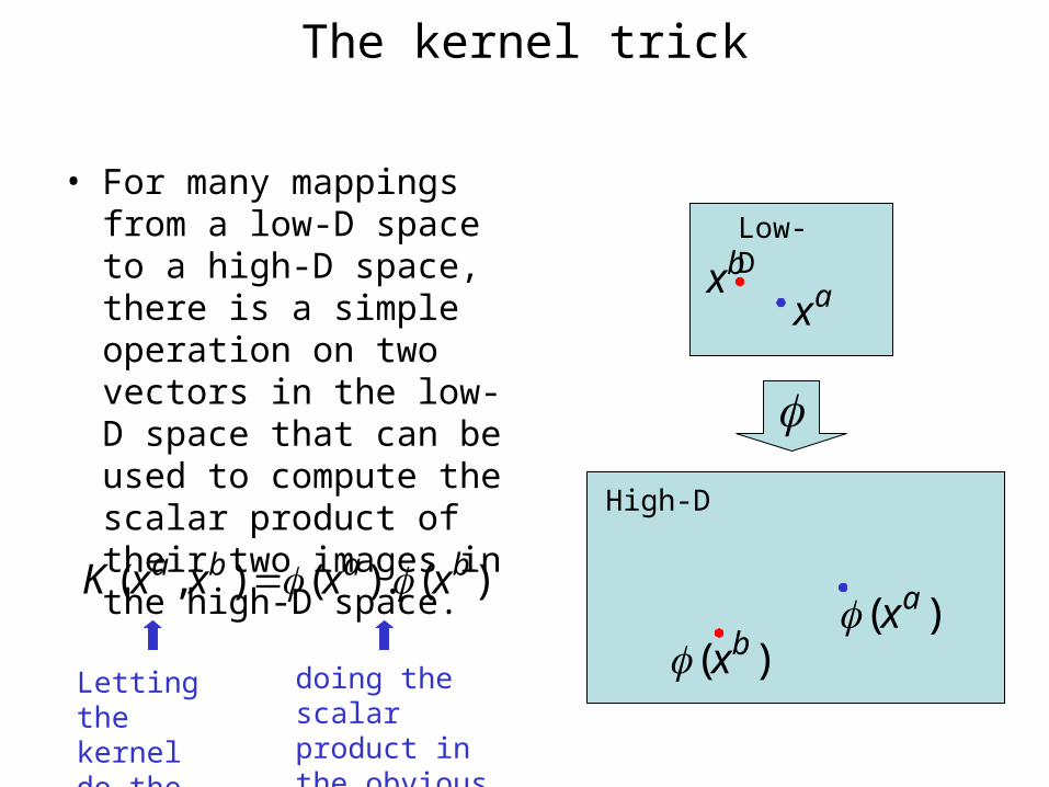
The kernel trick

• For many mappings from a low-D space to a high-D space, there is a simple operation on two vectors in the low-D space that can be used to compute the scalar product of their two images in the high-D space.

)(.)(),( baba xxxxK

Low-D

High-D

doing the scalar product in the obvious way

Letting the kernel do the work

ax

)( ax)( bx

bx

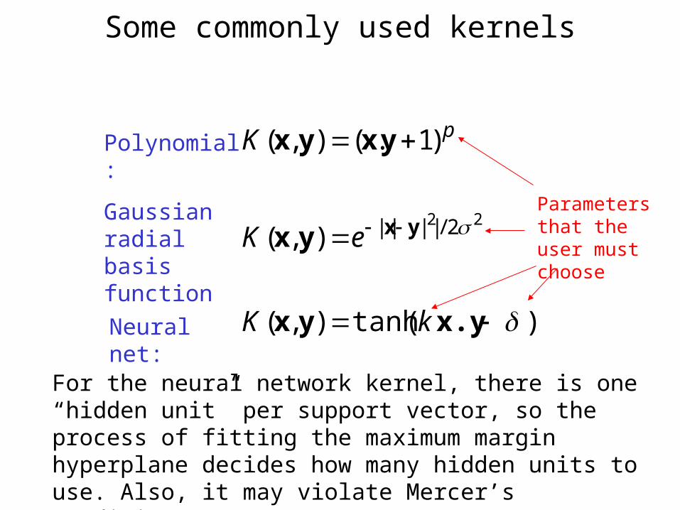
Some commonly used kernels

)(tanh),(

),(

)1.(),(

22 2/||||

x.yyx

yx

yxyx

yx

kK

eK

K pPolynomial:

Gaussian radial basis function

Neural net:

For the neural network kernel, there is one “hidden unit” per support vector, so the process of fitting the maximum margin hyperplane decides how many hidden units to use. Also, it may violate Mercer’s condition.

Parameters that the user must choose

Performance

• Support Vector Machines work very well in practice. – The user must choose the kernel function and its

parameters, but the rest is automatic.– The test performance is very good.

• They can be expensive in time and space for big datasets– The computation of the maximum-margin hyper-plane

depends on the square of the number of training cases.– We need to store all the support vectors.

• SVM’s are very good if you have no idea about what structure to impose on the task.

• The kernel trick can also be used to do PCA in a much higher-dimensional space, thus giving a non-linear version of PCA in the original space.

End Theory I

• 5 min Mindmapping• 10 min Break

Practice I

Learning

• Supervised (Classification)– Classification

• Decision tree

• SVM

Classification

• Use the iris.txt file for classification

• Follow along as we classify

Playtime

• Try to optimize the classification by playing around with the parameters

• Who can achieve the best accuracy in 15 min?

End Practice I

• 15 min break

Theory II

Holdout validation

• One way to validate your model is to fit your model on half your dataset (your “training set”) and test it on the remaining half of your dataset (your “test set”).

• If over-fitting is present, the model will perform well in your training dataset but poorly in your test dataset.

• Of course, you “waste” half your data this way, and often you don’t have enough data to spare…

Alternative strategies:

• Leave-one-out validation (leave one observation out at a time; fit the model on the remaining training data; test on the held out data point).

• K-fold cross-validation—what we will discuss today.

When is cross-validation used?

• Very important in microarray experiments (“p is larger than N”).

• Anytime you want to prove that your model is not over-fit, that it will have good prediction in new datasets.

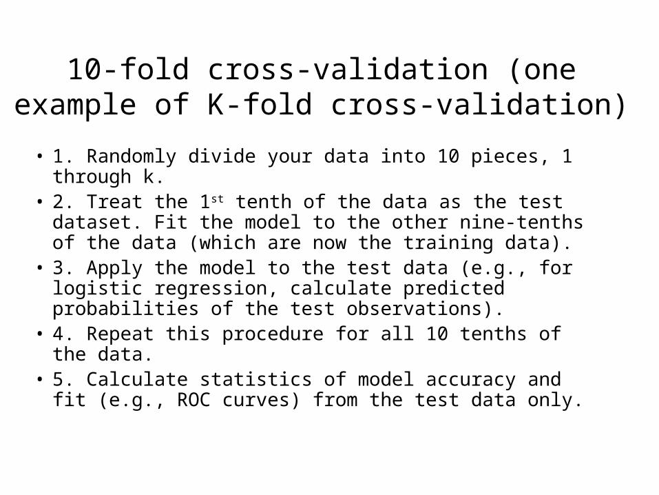
10-fold cross-validation (one example of K-fold cross-validation)

• 1. Randomly divide your data into 10 pieces, 1 through k.

• 2. Treat the 1st tenth of the data as the test dataset. Fit the model to the other nine-tenths of the data (which are now the training data).

• 3. Apply the model to the test data (e.g., for logistic regression, calculate predicted probabilities of the test observations).

• 4. Repeat this procedure for all 10 tenths of the data.• 5. Calculate statistics of model accuracy and fit (e.g.,

ROC curves) from the test data only.

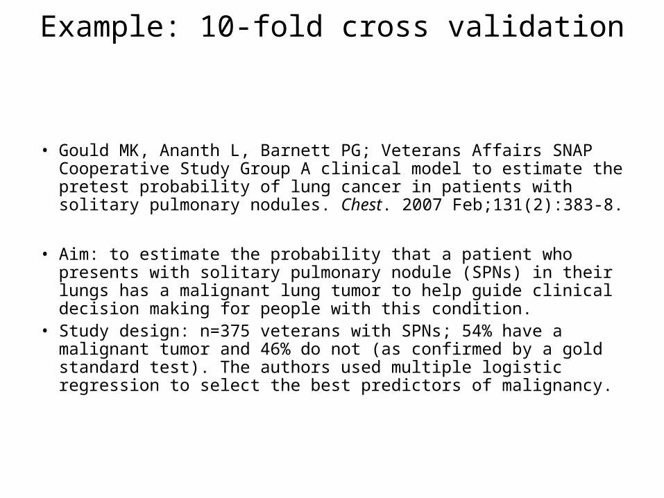
Example: 10-fold cross validation

• Gould MK, Ananth L, Barnett PG; Veterans Affairs SNAP Cooperative Study Group A clinical model to estimate the pretest probability of lung cancer in patients with solitary pulmonary nodules. Chest. 2007 Feb;131(2):383-8.

• Aim: to estimate the probability that a patient who presents with solitary pulmonary nodule (SPNs) in their lungs has a malignant lung tumor to help guide clinical decision making for people with this condition.

• Study design: n=375 veterans with SPNs; 54% have a malignant tumor and 46% do not (as confirmed by a gold standard test). The authors used multiple logistic regression to select the best predictors of malignancy.

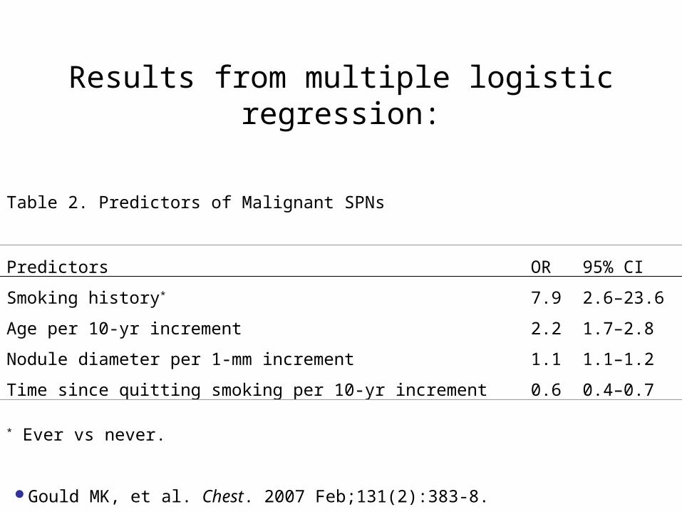
Results from multiple logistic regression:

Table 2. Predictors of Malignant SPNs

Predictors OR 95% CI

Smoking history* 7.9 2.6–23.6

Age per 10-yr increment 2.2 1.7–2.8

Nodule diameter per 1-mm increment 1.1 1.1–1.2

Time since quitting smoking per 10-yr increment 0.6 0.4–0.7

* Ever vs never.

Gould MK, et al. Chest. 2007 Feb;131(2):383-8.

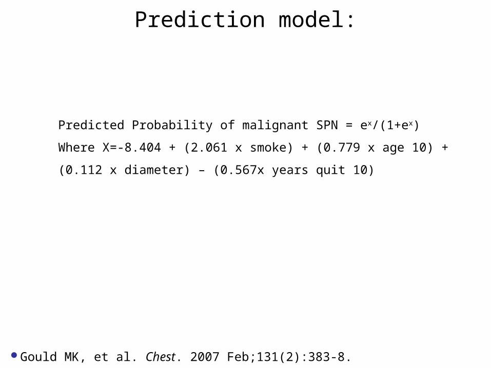
Prediction model:

Predicted Probability of malignant SPN = ex/(1+ex)

Where X=-8.404 + (2.061 x smoke) + (0.779 x age 10) +

(0.112 x diameter) – (0.567x years quit 10)

Gould MK, et al. Chest. 2007 Feb;131(2):383-8.

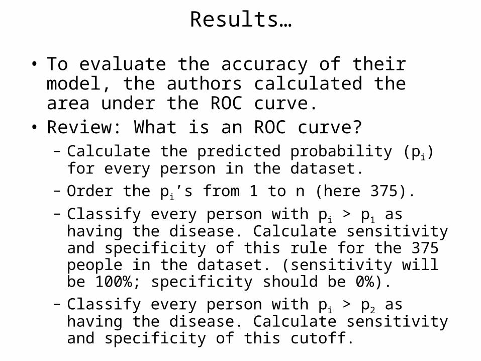
Results…

• To evaluate the accuracy of their model, the authors calculated the area under the ROC curve.

• Review: What is an ROC curve?– Calculate the predicted probability (pi) for every

person in the dataset.– Order the pi’s from 1 to n (here 375).– Classify every person with pi > p1 as having the

disease. Calculate sensitivity and specificity of this rule for the 375 people in the dataset. (sensitivity will be 100%; specificity should be 0%).

– Classify every person with pi > p2 as having the disease. Calculate sensitivity and specificity of this cutoff.

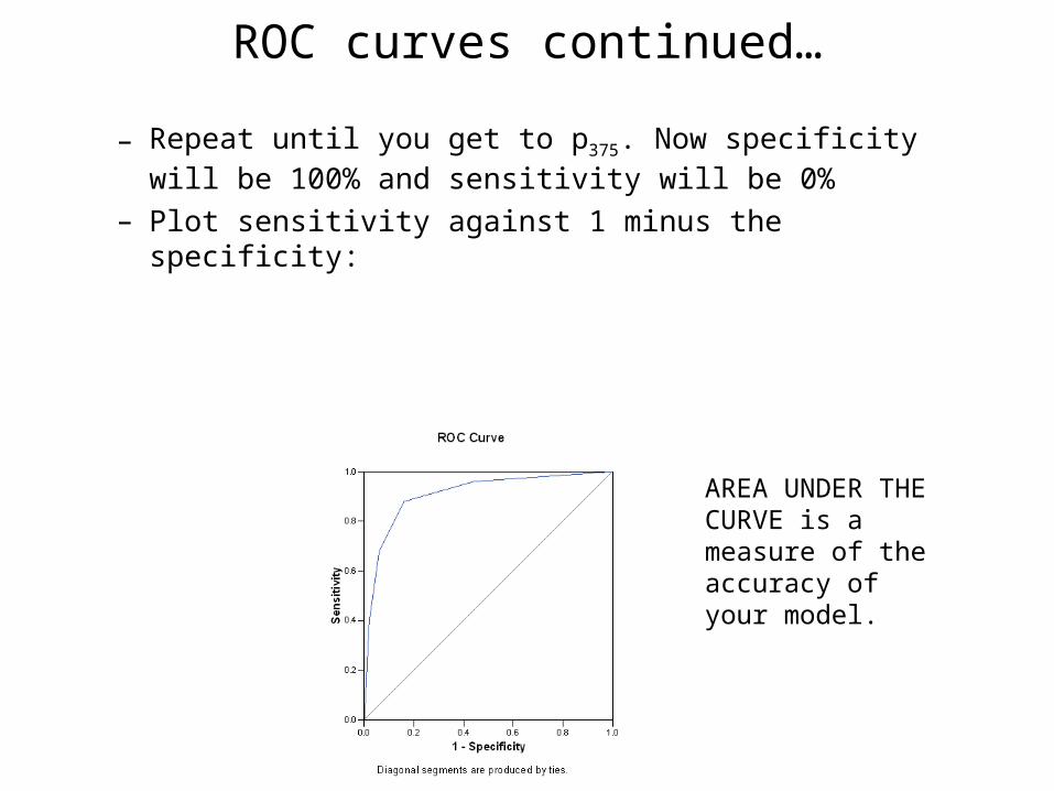
ROC curves continued…

– Repeat until you get to p375. Now specificity will be 100% and sensitivity will be 0%

– Plot sensitivity against 1 minus the specificity:

AREA UNDER THE CURVE is a measure of the accuracy of your model.

Results

• The authors found an AUC of 0.79 (95% CI: 0.74 to 0.84), which can be interpreted as follows:– If the model has no predictive power, you have a 50-50 chance

of correctly classifying a person with SPN.– Instead, here, the model has a 79% chance of correct

classification (quite an improvement over 50%).

A role for 10-fold cross-validation

• If we were to apply this logistic regression model to a new dataset, the AUC will be smaller, and may be considerably smaller (because of over-fitting).

• Since we don’t have extra data lying around, we can use 10-fold cross-validation to get a better estimate of the AUC…

10-fold cross validation

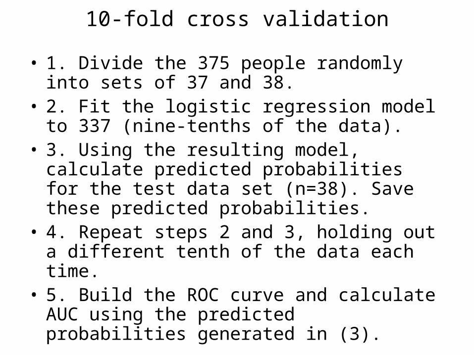
• 1. Divide the 375 people randomly into sets of 37 and 38.

• 2. Fit the logistic regression model to 337 (nine-tenths of the data).

• 3. Using the resulting model, calculate predicted probabilities for the test data set (n=38). Save these predicted probabilities.

• 4. Repeat steps 2 and 3, holding out a different tenth of the data each time.

• 5. Build the ROC curve and calculate AUC using the predicted probabilities generated in (3).

Results…

• After cross-validation, the AUC was 0.78 (95% CI: 0.73 to 0.83).

• This shows that the model is robust.

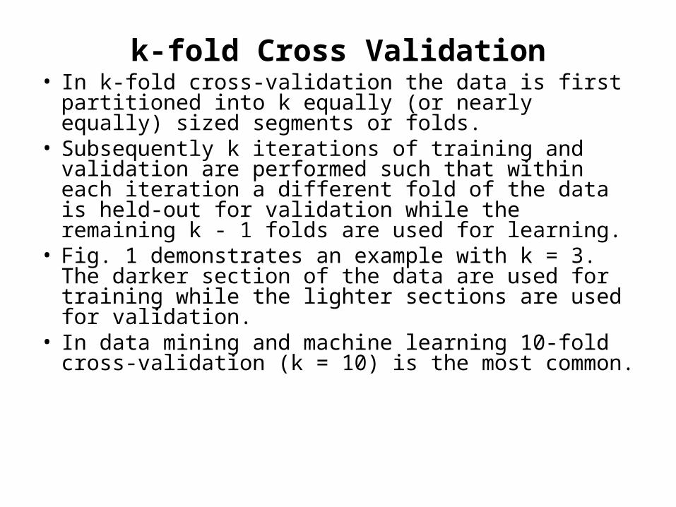
k-fold Cross Validation• In k-fold cross-validation the data is first

partitioned into k equally (or nearly equally) sized segments or folds.

• Subsequently k iterations of training and validation are performed such that within each iteration a different fold of the data is held-out for validation while the remaining k - 1 folds are used for learning.

• Fig. 1 demonstrates an example with k = 3. The darker section of the data are used for training while the lighter sections are used for validation.

• In data mining and machine learning 10-fold cross-validation (k = 10) is the most common.

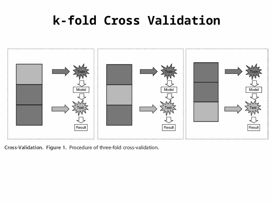
k-fold Cross Validation

Leave-One-Out Cross-Validation

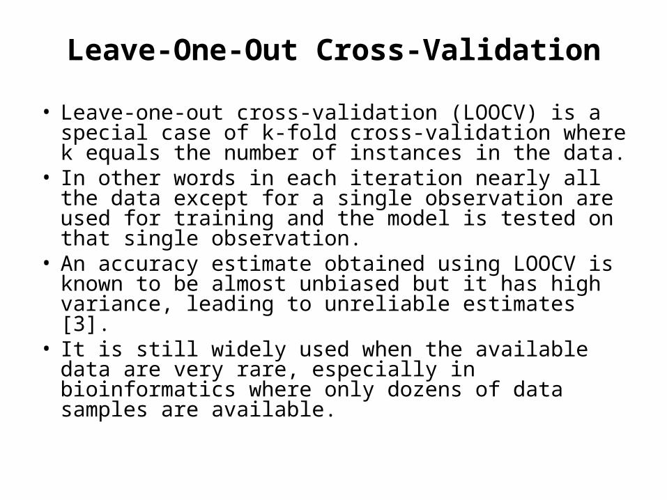
• Leave-one-out cross-validation (LOOCV) is a special case of k-fold cross-validation where k equals the number of instances in the data.

• In other words in each iteration nearly all the data except for a single observation are used for training and the model is tested on that single observation.

• An accuracy estimate obtained using LOOCV is known to be almost unbiased but it has high variance, leading to unreliable estimates [3].

• It is still widely used when the available data are very rare, especially in bioinformatics where only dozens of data samples are available.

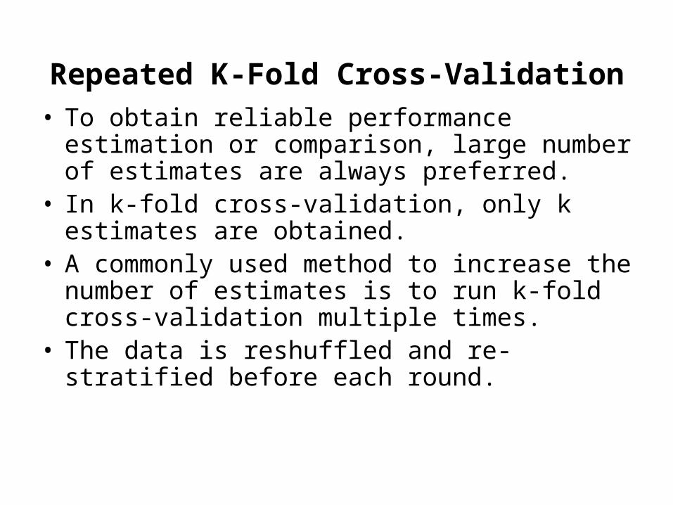
Repeated K-Fold Cross-Validation• To obtain reliable performance estimation or

comparison, large number of estimates are always preferred.

• In k-fold cross-validation, only k estimates are obtained.

• A commonly used method to increase the number of estimates is to run k-fold cross-validation multiple times.

• The data is reshuffled and re-stratified before each round.

Using Out-of-Sample Data

Holdout Data

Lift Curves & Gains Charts

Validation Data

Cross-Validation

Out-of-Sample Data

• Simplest idea: Divide data into 2 pieces.• Training Data: data used to fit model

• Test Data: “fresh” data used to evaluate model

• Test data contains: • actual target value Y

• model prediction Y*

• We can find clever ways of displaying the relation between Y and Y*.• Lift curves, gains charts, ROC curves…………

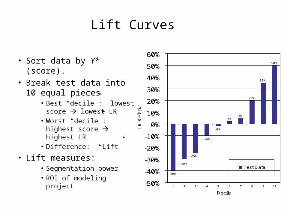
Lift Curves

• Sort data by Y* (score).• Break test data into 10

equal pieces • Best “decile”: lowest

score lowest LR• Worst “decile”: highest

score highest LR • Difference: “Lift”

• Lift measures:• Segmentation power• ROI of modeling project

-40%

-10%

-2%

2%5%

20%

35%

50%

-25%

-30%

-50%

-40%

-30%

-20%

-10%

0%

10%

20%

30%

40%

50%

60%

1 2 3 4 5 6 7 8 9 10

Decile

LR

Re

lativ

ity

Test Data

Lift Curves: Practical Benefits

• What do we really care about when we build a model?– High R2, etc?– …or increased profitability?

• Paraphrase of Michael Berry:

Success is measured in dollars… R2, misclassification rate… don’t matter.

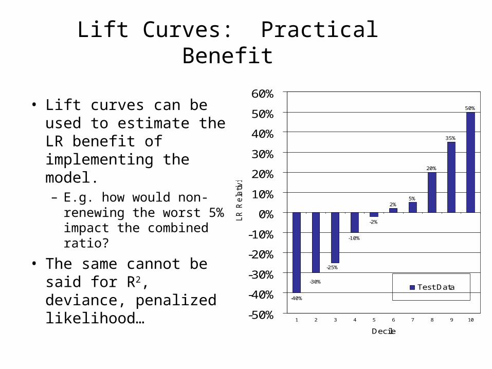
Lift Curves: Practical Benefit

• Lift curves can be used to estimate the LR benefit of implementing the model.– E.g. how would non-

renewing the worst 5% impact the combined ratio?

• The same cannot be said for R2, deviance, penalized likelihood…

-40%

-10%

-2%

2%5%

20%

35%

50%

-25%

-30%

-50%

-40%

-30%

-20%

-10%

0%

10%

20%

30%

40%

50%

60%

1 2 3 4 5 6 7 8 9 10

Decile

LR

Re

lativ

ity

Test Data

Lift Curves: Other Benefits

• Allows one to easily compare multiple models on out-of-sample data.

– Which is the best technique? • GLM, decision tree, neural net, MARS….?

– Other modeling options: • Optimal predictive variables, target variables…

• Lends itself to iterative model-building process, “controlled experiments”.

– Need for final model validation.

Lift Curves: Other Benefits

• Some times traditional statistical measures don’t really give a feel for how successful the model is.

– Personal line regression model fit on many million records.• R2 ≈ .0002• But excellent lift curve

– Many traditional statisticians would say we’re wasting our time.– Are we?

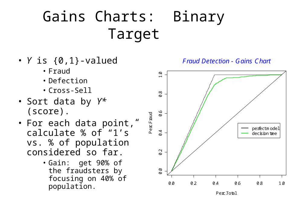
Gains Charts: Binary Target

• Y is {0,1}-valued• Fraud• Defection• Cross-Sell

• Sort data by Y* (score).• For each data point,

calculate % of “1’s” vs. % of population considered so far.

• Gain: get 90% of the fraudsters by focusing on 40% of population.

0.0 0.2 0.4 0.6 0.8 1.0

0.0

0.2

0.4

0.6

0.8

1.0

Perc.Total

Pe

rc.F

rau

d

perfect modeldecision tree

Fraud Detection - Gains Chart

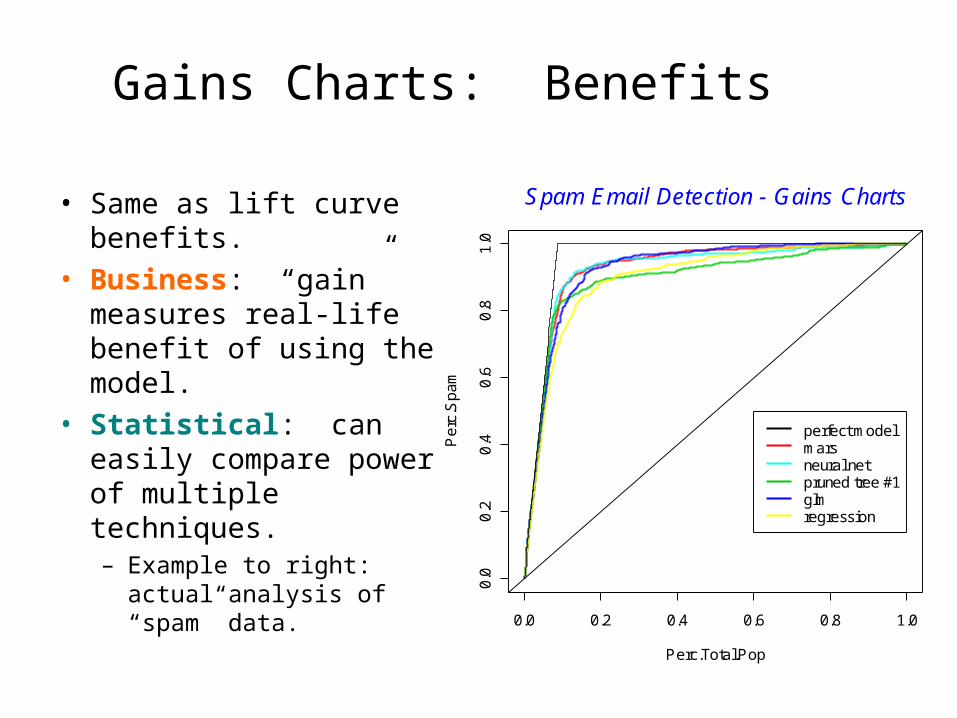
Gains Charts: Benefits

• Same as lift curve benefits.

• Business: “gain” measures real-life benefit of using the model.

• Statistical: can easily compare power of multiple techniques.– Example to right: actual

analysis of “spam” data.

0.0 0.2 0.4 0.6 0.8 1.0

0.0

0.2

0.4

0.6

0.8

1.0

Perc.Total.Pop

Pe

rc.S

pa

mperfect modelmarsneural netpruned tree #1glmregression

Spam Email Detection - Gains Charts

Model Selection vs. Validation

• Suppose we’ve gone though an iterative model-building process.• Fit several models on the training data

• Tested/compared them on the test data

• Selected the “best” model

• The test lift curve of the best model might still be overly optimistic.• Why: we used the test data to select the best model.

• Implicitly, it was used for modeling.

Validation Data

• It is therefore preferable to divide the data into three pieces:• Training Data: data used to fit model

• Test Data: “fresh” data used to select model

• Validation Data: data used to evaluate the final, selected model.

• Train/Test data is iteratively used for model building, model selection.• During this time, Validation data set aside and not touched.

Validation Data

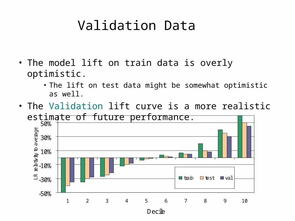
• The model lift on train data is overly optimistic.• The lift on test data might be somewhat optimistic as well.

• The Validation lift curve is a more realistic estimate of future performance.

-50%

-30%

-10%

10%

30%

50%

1 2 3 4 5 6 7 8 9 10

Decile

LR

re

lativ

ity to

ave

rag

e

train test val

Validation Data

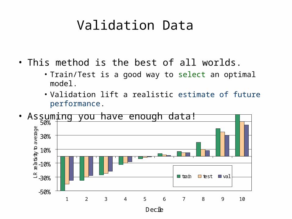
• This method is the best of all worlds.• Train/Test is a good way to select an optimal model.• Validation lift a realistic estimate of future performance.

• Assuming you have enough data!

-50%

-30%

-10%

10%

30%

50%

1 2 3 4 5 6 7 8 9 10

Decile

LR

re

lativ

ity to

ave

rag

e

train test val

Cross-Validation

• What if we don’t have enough data to set aside a test dataset?

• Cross-Validation:• Each data point is used both as train and test data.

• Basic idea:• Fit model on 90% of the data; test on other 10%.

• Now do this on a different 90/10 split.

• Cycle through all 10 cases.

• 10 “folds” a common rule of thumb.

Ten Easy Pieces

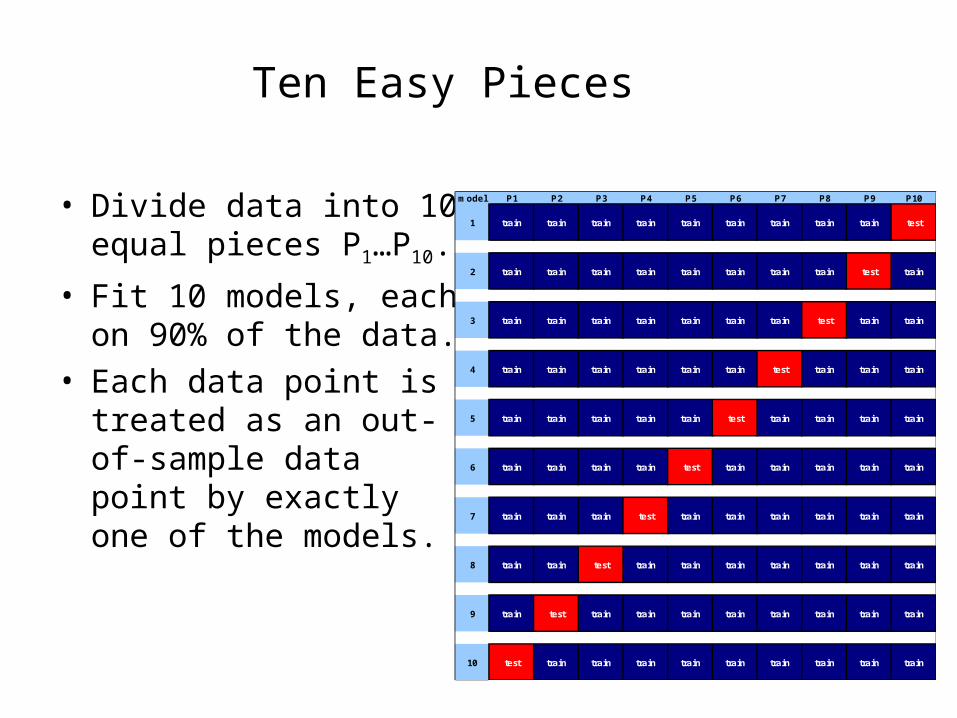
• Divide data into 10 equal pieces P1…P10.

• Fit 10 models, each on 90% of the data.

• Each data point is treated as an out-of-sample data point by exactly one of the models.

model P1 P2 P3 P4 P5 P6 P7 P8 P9 P10

1 train train train train train train train train train test

2 train train train train train train train train test train

3 train train train train train train train test train train

4 train train train train train train test train train train

5 train train train train train test train train train train

6 train train train train test train train train train train

7 train train train test train train train train train train

8 train train test train train train train train train train

9 train test train train train train train train train train

10 test train train train train train train train train train

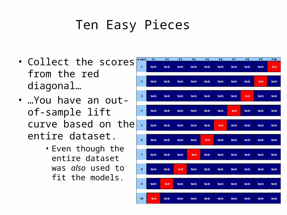
Ten Easy Pieces

• Collect the scores from the red diagonal…

• …You have an out-of-sample lift curve based on the entire dataset.

• Even though the entire dataset was also used to fit the models.












Uses of Cross-Validation

• Model Evaluation• Collect the scores from the ‘red boxes’ and generate a lift curve or

gains chart.• Simulates the effect of using the train/test method.• End run around the “small dataset” problem.

• Model Selection• Index your models by some parameter α.

» # variables in a regression» # neural net nodes» # leaves in a tree

• Choose α value resulting in lowest CV error rate.

Model Selection Example

• Use CV to select an optimal decision tree.• Built into the Classification & Regression Tree (CART)

decision tree algorithm.• Basic idea: “grow the tree” out as far as you can….

Then “prune back”.• CV: tells you when to stop pruning.

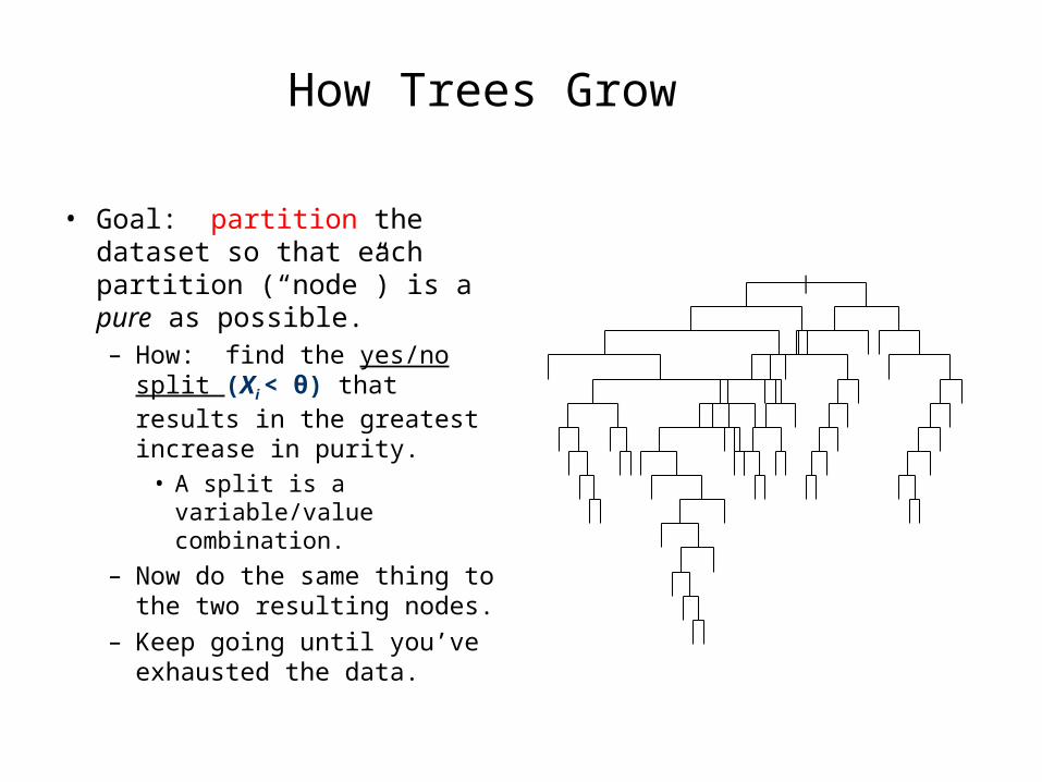
How Trees Grow

• Goal: partition the dataset so that each partition (“node”) is a pure as possible.– How: find the yes/no split

(Xi < θ) that results in the greatest increase in purity.

• A split is a variable/value combination.

– Now do the same thing to the two resulting nodes.

– Keep going until you’ve exhausted the data.

|

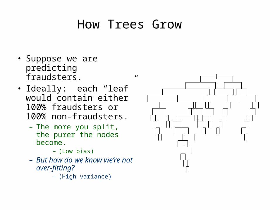
How Trees Grow

• Suppose we are predicting fraudsters.

• Ideally: each “leaf” would contain either 100% fraudsters or 100% non-fraudsters.– The more you split, the

purer the nodes become.– (Low bias)

– But how do we know we’re not over-fitting?

– (High variance)

|

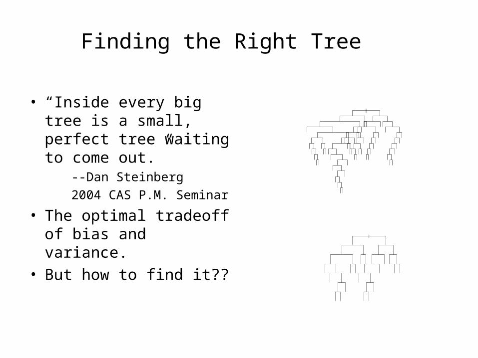
Finding the Right Tree

• “Inside every big tree is a small, perfect tree waiting to come out.”

--Dan Steinberg

2004 CAS P.M. Seminar

• The optimal tradeoff of bias and variance.

• But how to find it??

|

|

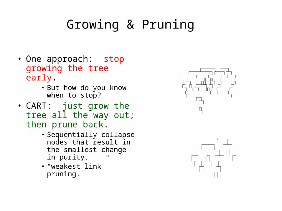
Growing & Pruning

• One approach: stop growing the tree early.

• But how do you know when to stop?

• CART: just grow the tree all the way out; then prune back.

• Sequentially collapse nodes that result in the smallest change in purity.

• “weakest link” pruning.

|

|

Cost-Complexity Pruning

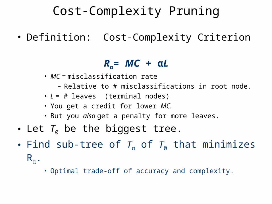
• Definition: Cost-Complexity Criterion

Rα= MC + αL• MC = misclassification rate

– Relative to # misclassifications in root node.

• L = # leaves (terminal nodes)

• You get a credit for lower MC.

• But you also get a penalty for more leaves.

• Let T0 be the biggest tree.

• Find sub-tree of Tα of T0 that minimizes Rα.• Optimal trade-off of accuracy and complexity.

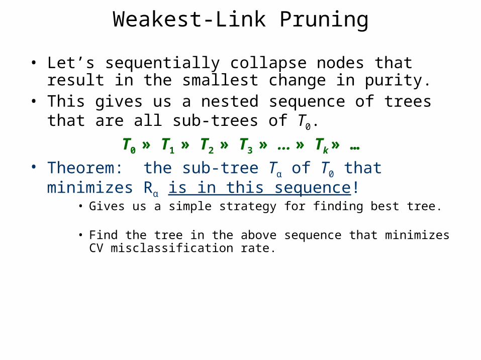
Weakest-Link Pruning

• Let’s sequentially collapse nodes that result in the smallest change in purity.

• This gives us a nested sequence of trees that are all sub-trees of T0.

T0 » T1 » T2 » T3 » … » Tk » …• Theorem: the sub-tree Tα of T0 that minimizes Rα is in

this sequence! • Gives us a simple strategy for finding best tree.• Find the tree in the above sequence that minimizes CV

misclassification rate.

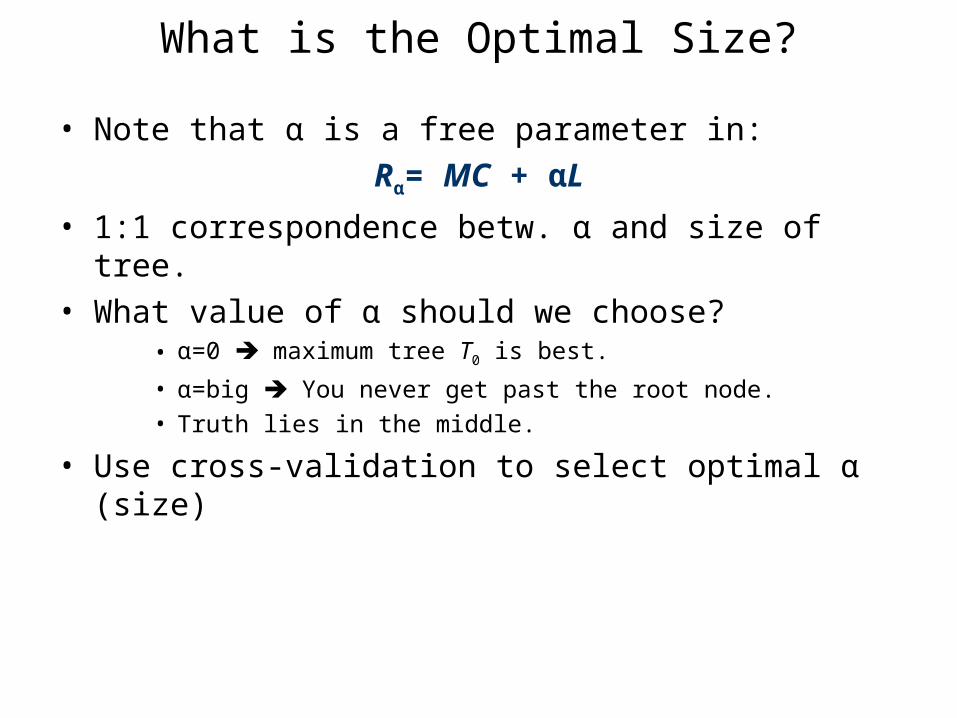
What is the Optimal Size?

• Note that α is a free parameter in:

Rα= MC + αL

• 1:1 correspondence betw. α and size of tree.• What value of α should we choose?

• α=0 maximum tree T0 is best.

• α=big You never get past the root node.

• Truth lies in the middle.

• Use cross-validation to select optimal α (size)

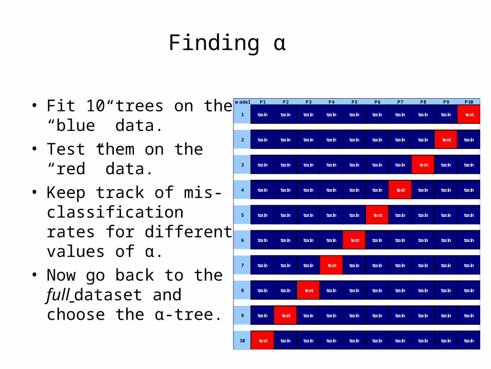
Finding α

• Fit 10 trees on the “blue” data.

• Test them on the “red” data.

• Keep track of mis-classification rates for different values of α.

• Now go back to the full dataset and choose the α-tree.












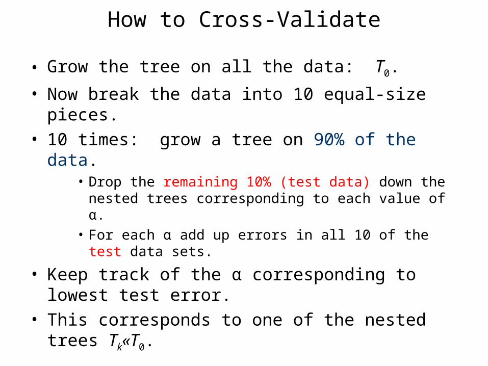
How to Cross-Validate

• Grow the tree on all the data: T0.

• Now break the data into 10 equal-size pieces.

• 10 times: grow a tree on 90% of the data.• Drop the remaining 10% (test data) down the nested trees

corresponding to each value of α.• For each α add up errors in all 10 of the test data sets.

• Keep track of the α corresponding to lowest test error.

• This corresponds to one of the nested trees Tk«T0.

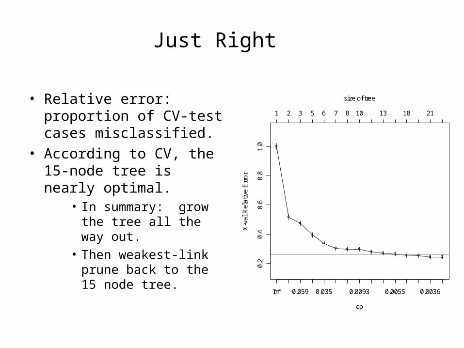
Just Right

• Relative error: proportion of CV-test cases misclassified.

• According to CV, the 15-node tree is nearly optimal.

• In summary: grow the tree all the way out.

• Then weakest-link prune back to the 15 node tree.

cp

X-v

al R

ela

tive

Err

or

0.2

0.4

0.6

0.8

1.0

Inf 0.059 0.035 0.0093 0.0055 0.0036

1 2 3 5 6 7 8 10 13 18 21

size of tree

End Theory II

• 5 min Mindmapping• 10 min Break

Practice II

Classification

• Use the orangeexample file for classification

• We are interested if we can distinguish between miRNAs and random sequences with the selected features

• Try yourself

• Competition, who achieves the best accuracy in the next 30 min?

Documents

Computational Biology Lecture Slides Week 10 Classification (some parts taken from Introduction to Data Mining by Tan, Steinbach, Kumar)