QUARTERLY OF APPLIED MATHEMATICS 51
APRIL, 1972
SPECIAL ISSUE: SYMPOSIUM ON"THE FUTURE OF APPLIED MATHEMATICS"
DATA ANALYSIS, COMPUTATION AND MATHEMATICS*
BY
JOHN W. TUKEY
Bell Telephone Laboratories, Murray Hill, and Princeton University
Abstract. "Data analysis" instead of "statistics" is a name that allows us to use
probability where it is needed and avoid it when we should. Data analysis has to analyze
real data. Most real data calls for data investigation, while almost all statistical theory
is concerned with data processing. This can be borne, in part because large segments
of data investigation are, by themselves, data processing. Summarizing a batch of
20 numbers is a convenient paradigm for more complex aims in data analysis. A partic-
ular summary, highly competitive among those known and known about in August 1971,
is a hybrid between two moderately complex summaries. Data investigation comes
in three stages: exploratory data analysis (no probability), rough confirmatory data
analysis (sign test procedures and the like), mustering and borrowing strength (the best
of modern robust techniques, and an art of knowing when to stop). Exploratory data
analysis can be improved by being made more resistant, either with medians or with
fancier summaries. Rough confirmatory data analysis can be improved by facing up to
the issues surrounding the choice of what is to be confirmed or disaffirmed. Borrowing
strength is imbedded in our classical procedures, though we often forget this. Mustering
strength calls for the best in robust summaries we can supply. The sampling behavior
of such a summary as the hybrid mentioned above is not going to be learned through
the mathematics of certainty, at least as we know it today, especially if we are realistic
about the diversity of non-Gaussian situations that are studied. The mathematics of
simulation, inevitably involving the mathematically sound "swindles" of Monte Carlo,
will be our trust and reliance. I illustrate results for a few summaries, including the
hybrid mentioned above. Bayesian techniques are still a problem to the author, mainly
because there seems to be no agreement on what their essence is. From my own point
of view, some statements of their essence are wholly acceptable and others are equally
unacceptable. The use of exogeneous information in analyzing a given body of data is
a very different thing (a) depending on sample size and (b) depending on just how the
exogeneous information is used. It would be a very fine thing if the questions that
practical data analysis has to have answered could be answered by the mathematics
of certainty. For my own part, I see no escape, for the next decade or so at least, from
a dependence on the mathematics of simulation, in which we should heed von Neumann's
aphorism as much as we can.
As one who was once a Brown chemist, I am happy to be back, and honored to
take part in this celebration.
* Prepared in part in connection with research at Princeton University sponsored by the Army
Research Office (Durham).
52 JOHN W. TUKEY
1. Names, what is in them? My title speaks of "data analysis" not "statistics",
and of "computation" not "computing science"; it does speak of "mathematics", but
only last. Why? The answers to these questions need a substructure of understanding
to which this talk will be devoted.
My brother-in-squared-law, Francis J. Anscombe [2, footnote to page 3] has com-
mented on my use of "data analysis" in the following words:
Whereas the content of Tukey's remarks is always worth pondering, some
of his terminology is hard to take. He seems to identify "statistics" with the
grotesque phenomenon generally known as "mathematical statistics", and finds
it necessary to replace "statistical analysis" by "data analysis". The change is a
little unfortunate because the statistician's data are the observer's facta, and
sometimes observer and statistician are the same person, in which case he is no
doubt primarily observer. Perhaps "facta analysis" is the answer.
One reason for being careful about names has been made clear by Gower and Ross
[5, pages 55-56] who say:
It is often argued that for a method to be statistical it should have some
probabilistic basis, but many methods profitably used by practicing statisticians
do not have this basis. In others (for example, analysis of variance) it is arguable
that the probabilistic features are not fundamental to the method.
Many of those who use the words "data analysis" adhere to the view that "It is well
to understand what you can do before you learn how to measure how well you seem
able to do it" [13]. I shall stick to this attitude today, and shall continue to use the words
"data analysis", in part to indicate that we can take probability seriously, or leave it
alone, as may from time to time be appropriate or necessary.
Data analysis is in important ways an antithesis of pure mathematics. I well remem-
ber a conversation in 1945 or 1946 with the late Walther Mayer, then at the Institute for
Advanced Study, who wondered at my interest in continuing at Bell Telephone Lab-
oratories, which he thought of as quite applied. He indicated how important it was for
him to know "that if I say gik has certain properties, it really does". He knew that such
a fiat need not rule an application. A similar antithesis holds for many, perhaps all,
branches of applied mathematics, but often in a very much weaker form.
The practicing data analyst has to analyze data. The techniques that the theorizing
data analyst—-often the same person—thinks about have to be used to analyze data.
It is never enough to be able to analyze simplified cases.
The membrane theory of shells did not have to design buildings, though hopefully
it guided their designing. The solution to the travelling salesman problem did not have
to take account of airline schedules. Early work in population genetics did not have to
consider the geographic structure and connectivity of each important type of ecological
niche. One analogue to these latter fields, where oversimplification has taught us much,
is statistical theory, which ought to do its share in guiding data analysis.
All too often, statistical theory is miscalled mathematical statistics, about which
too many practitioners (even some of them Englishmen!) take the dangerous view that
work can be good mathematical statistics without being either good mathematics or
good statistics. (Fortunately the number who do this are few.)
DATA ANALYSIS, COMPUTATION AND MATHEMATICS 53
It will be our purpose to try to see how data analysis is reasonably practiced, how
statistical theory helps to guide it, and why computing will have to play a major role
in the development of newer and deeper guidance.
2. Flow charts, with or without switches? Procedures, theoretical or actual, for
passing from data to results fall naturally into two broad categories:
1. Those whose flow patterns involve significant switching points where the details
of the data determine, often by human intervention, what is to be done next to that
particular set of data—-these are well called "data investigation".
2. Those whose flow patterns involve no significant data-driven switching (at least
to the hasty eye)—these we shall call "data processing".
It is a harsh fact, but true, that most data call for data investigation, while almost
all statistical theory is concerned with data processing. Harsh, but not quite as harsh
as it might seem.
I recall Professor Ducasse giving a paper to the philosophy seminar, a few hundred
yards west of here in Rhode Island Hall, in which he said deduction and induction could
be completely separated, that each of us was doing one or the other, not both. The tides
of controversy rose high, but ebbed away again once we all recognized that he meant
this separation to be instant by instant, rather than minute by minute or process by
process.
Statistical theory can, has, and will give very useful guidance to data investigation.
In most cases, however, this will be because its results are used to guide only some part,
smaller or larger, of the data-investigative process, a part that comes at least close
to being data processing.
If statistical theory really encompassed all the practical problems of data analysis,
and if we were able to implement all its derived precepts effectively, then there would
be no data investigation, only data processing. We are far from that tarnished Utopia
today—-and not likely to attain it tomorrow.
3. Summarizing a batch—in various styles. The oldest problem of data analysis
is summarizing a batch of numbers—-where a batch is a set of numbers, all of which
are taken as telling us about the same thing. When these numbers are the ages at death
for twelve children of a single parentage, they are not expected to be the same and often
differ widely. When these numbers are the precisely measured values of the same physical
constant obtained by twelve skilled observers they again ought not to be expected to
be the same—-though too many forget this—-but they often differ very little. In either
case summarization may be in order.
Until rather late in our intellectual history [4], summarization of such a set of obser-
vations was by picking out a good observation—and, I fear, claiming that it was the
best. By the time of Gauss, however, the use of the arithmetic mean was common,
and much effort was spent on trying to show that it was, in fact, the best. To be best
required that what was chosen as a summary could be compared with some "reality"
beyond the data. For this to be sensible, there had to be a process that generated varying
sets of data. The simplest situation that would produce sets of data showing many of
the idiosyncrasies of real data sets was random sampling from an infinite population.
Thus the supposed quality of the arithmetic mean was used to establish the Gaussian
distribution—-and the supposed reality of the Gaussian distribution was used to es-
tablish the optimal nature of the arithmetic mean. No doubt the circularity was clear
to many who worked in this field, but there may have been more than a trace of the
54 JOHN W. TUKEY
attitude expressed by Hermann Weyl, who, when asked about his attitude to classical
and intuitionistic mathematics, said that he was only certain of what could be established
by intuitionistic methods, but that he liked to obtain results. It would have been a
great loss for mathematics had "the great, the noble, the holy Hermann" taken any
other view.
By the early 1930s, when I first met it, the practice of data analysis, at least in the
most skilled hands, had advanced to the point where summarization was data investiga-
tion, in the sense that apparently well-behaved data would be summarized by its means,
while apparently ill-behaved sets of numbers would be summarized in a more resistant
way, perhaps by their medians. Such a branching need not mean that the summary
cannot be a fixed function of the data; it does mean that this fixed function is not going
to be completely simple to write down.
If we can specify a general rule for the branching, we have effectively chosen a fixed
function that pleases us. When we go further and use this function routinely, we are
likely to reconvert summarization from data investigation to data processing. This will
surely be true if any switch-like character of the fixed function is sufficiently concealed.
Even when this is done, however, the microprocess of summarization is still likely to be
contained in a macroprocess of data investigation.
It has been nearly 30 years since I met data analysts smart enough to avoid the
arithmetic means most of the time. Yet our books and lectures still concentrate on it,
as if it were the good thing to do, and almost all our more sophisticated calculations—•
analyses of variance, multiple regressions (even factor analyses)—use analogues of the
arithmetic mean rather than analogues of something safer and better. Progress has
been slow.
4. An example—the summary of the month. Since these lines are written on 31
August, I can designate a particular form of summary as the summary for August 1971
without claiming too much about the future, about how it will compare with those
summaries that will come to our attention in September, and in the months to come.
For simplicity—and because I happen to have better numbers for this special case—I
am going to restrict the definition to batches of 20. (A reasonable extension to all n is
easy; a really good extension may take thought and experimentation.)
Let us then consider 3 different summaries (central values) of 20 x<'s (i — 1, 2, • • • , 20),
namely CXO = ^(21B) + |(C02), where 21B is defined implicitly, following a pattern
proposed by Hampel, while CO2 is a sit mean (where "sit" is for skip-mto-<rim). (21B
was chosen here for simplicity of mathematical description; a closely related estimate-
perhaps the one presently designated 21E, the first step of a Newton-Raphson approxi-
mation to 215, starting at C02—would tend to save computing time without appreciable
loss of performance.)
Let be a polygonal function of a real variable defined by:
M, 0 < \x\ < 2.1
2.1, 2.1 < |a;| < 4.1
^21 b(x) = (sign x)>
(2.1) 9-1 W , 4.1 < |x| < 9.1
0, 9.1 < \x\
DATA ANALYSIS, COMPUTATION AND MATHEMATICS 55
Then the value T of the estimate 21B is the solution of
Z hU(.x< - T)/s) = 0,i
where s is the median of the absolute deviations \x{ — x\ of the £; from their medians x.
(Replacing 2.1 etc. by 2.0 etc. would cost little. Results happen to be available for 2.1.)
Let next x(i) be the x, rearranged in increasing order so that x(i) < x(j) for i < j,
where i and j run from 1 to 20. Let the hinges be L = |x(5) + Jx(6), U = |x(15) +
%x(l6) (these are a form of quartile), and let the corners be C" = L — 2(U — L) =
SL — 2U, C* = U + 2(U — L) = 3(7 — 2L. Identify and count any x(i) that are
<C~ or >C+. Such values will be called "detached". To calculate the estimate C02,
proceed as follows:
1) if no observations are detached, form the mean of all observations.
2) if exactly one observation is detached, set it aside (skipping), and then set aside
two more at each end of the remaining list (trimming); form the mean of those not set
aside (here 15 in number).
3) if more than one observation is detached, set them aside (skipping), and then set
aside 4 more at each end of the remaining list (trimming); form the mean of those not
set aside (here 10 to 4 in number).
We shall return below to assessing the quality of these three estimates. Once we do,
it will be very hard to justify the arithmetic mean as a way of summarizing batches
(specifically for a batch of 20 numbers, actually for batches of more than 2 or perhaps 3).
The switching character of C02 is overt, that of 21B is covert. Both, as we shall see
later, perform well, while their mean, CXO, performs even better. Once a general com-
puting routine is coded, and we agree to use CXO "come hell or high water", which
would not be unwise in August or September 1971, we will (or would) have made this
kind of summarization into data processing again, at least for a time. If, as is so often
the case, however, we need to look at the data to see whether we want to summarize
x = y, x = \/y or x = log y, where y represents the numbers given to us, this piece of
data processing, called summarization, is still embedded in an only slightly larger piece
of data investigation.
The class of estimators to which 215 belongs has been called "hampels" [1] and
that to which C02 belongs has been called "sit means". It is thus natural to call the
class to which CXO belongs "sitha estimates". The best comment about such estimates
that I know of was made 75 years in advance by Rudyard Kipling (1897) who wrote
" 'sitha', said he softly, 'thot's better than owt,' ..
We are, of course, quite likely, as we learn more, to come to like some other sitha
estimate even better than CXO.
5. Three stages—of data investigation. As we come to think over the process of
analyzing data, when done well, we can hardly fail to identify the unrealism of the
descriptions given or implied in our texts and lectures. The description I am about to
give emphasizes three kinds of stages. It is more realistic than the description we are
accustomed to but we dare not think it (or anything else) the ultimate in realism.
The first stage is exploratory data analysis, which does not need probability, signi-
ficance, or confidence, and which, when there is much data, may need to handle only
either a portion or a sample of what is available. That there is still much to be said and
56 JOHN W. TUKEY
that there are new simple techniques to be developed is testified to by three volumes
of a book now in a limited preliminary edition [13] which deals only with the simpler
questions, leaving multiple regression and related questions for later treatment.
The second stage is probabilistic. Rough confirmatory data analysis asks, perhaps
quite crudely: "With what accuracy are the appearances already found to be believed?"
Three answers are reasonable:
1. The appearances are so poorly defined that they can be forgotten (at least as
evidence though probably not as clues).
2. The appearances are marginal (so that crude analysis may not suffice and a more
careful analysis is called for).
3. The appearances are well-determined (when we may, but more often do not,
have grounds for a more careful analysis).
Among the key issues of such a second stage are the issues of multiplicity: How many
things might have been looked at? How many had a real chance to be looked at? How
should the multiplicity decided upon, in answer to these questions, affect the resulting
confidence sets and significance levels? These are important questions; their answers
can affect what we think the data has shown.
It will only be after we have become used to dealing with the issues of multiplicity
that we will be psychologically ready to deal effectively with correlated estimates, to
recognize in particular (a) that the higher the correlation the less the chance—not the
greater—-of one or more accidental significances and (b) that correlation of fluctuations
need imply nothing as to whether the real effects measured by one calculated quantity
will in any way "leak" into other calculated quantities. Leakage of fluctuation and
leakage of effect need not go together, though they sometimes do.
When the result of the second stage is marginal, we need a third stage, in which we
wish to muster whatever strength the data before us possesses that bears directly on the
question at issue—and in which we often also want to borrow strength from either other
aspects of the same body of data or from other bodies of data. It is at this stage of
"mustering and borrowing strength" that we require our best statistical techniques.
Medians may be quite good enough for our rough confirmatory analysis, but if we have
good robust measures of location, such as CXO, they are needed in mustering and
borrowing strength. (For more on the three stages see [1].)
To argue, as we have implicitly done so often in the past, that—(1) all data requires
mustering and borrowing of strength and (2) this can—-nay should—be done without
any exploratory data analysis—-is surely at least one of the minor heights of unrealism.
Trying to make what needs to be data investigation into data processing that really
meets our needs involves many new ideas, and ideas come slowly.
6. Improvements—exploratory. In improving exploratory data analysis, we need
to find new questions to ask of the data (probably the hardest task), and new ways to
ask old questions. Throughout, arithmetic as a basis for preparing pictures is likely to be
the keynote. It is most important that we see in the data those things we do not expect—•
pictures help us in this far more than numbers, though we can gain a lot by just which
numbers we use.
Let us consider one case where new numbers can help a lot. If x(i, j) is given for
i = 1 to r, j = 1 to c, and if the various means, satisfying
c-x(i, •) = E4i), r-x{%, j) = 2lx(i,j), cr-x(#, ®) = X x(i, j),
DATA ANALYSIS, COMPUTATION AND MATHEMATICS 57
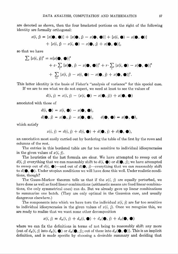
are denoted as shown, then the four bracketed portions on the right of the following
identity are formally orthogonal:
x(i, j) = [x(#, #)] + [z(#, J) - z(#, #)] + [x{i, •) - x{%, O)]
+ [x(i, j) - x(i©) - s(#, j) + x(&, #)],
so that we have
H [x(i, i)]2 = rc[x{%, #)]2
+ C-22 W#, 3) - x(9, #)]2 + r-X) [x(i, •) - z(#, #)]2I *'
+ X) b0"> i) - x(i, •) - z(#, i) + x(%, ®)]2.
This latter identity is the basis of Fisher's "analysis of variance" for this special case.
If we are to see what we do not expect, we need at least to see the values of
d(i, j) = x(i, j) - (x(i, •) - .t(®, j)) + x(t, •)
associated with those of
d(i, •) = x{i, ®) - ©),
dC, j) = x(9, j) - x(9, •), d(9, •) = x(9, •),
which satisfy
x(i, j) = d(i, j) + d(i, •) + d(#, j) + d(0, •),
an association most easily carried out by bordering the table of the first by the rows and
columns of the rest.
The entries in this bordered table are far too sensitive to individual idiosyncrasies
in the given values of x(i, j).
The heuristics of the last formula are clear. We have attempted to sweep out of
d(i, j) everything that we can reasonably shift to d(i, @) or d(%, j); we have attempted
to sweep out of d(i, %)—and out of d(0, j)—'everything that we can reasonably shift
to d(#, #). Under Utopian conditions we will have done this well. Under realistic condi-
tions, though?
The Gauss-Markov theorem tells us that if the x(i, j) are equally perturbed, we
have done as well as fixed linear combinations (arithmetic means are fixed linear combina-
tions, the only symmetrical ones) can do. But we already gave up linear combinations
to summarize one batch. (They are only optimal in the Gaussian case, and usually
dangerous elsewhere.)
The components into which we have torn the individual x(i, j) are far too sensitive
to individual idiosyncrasies in the given values of x(i, j). Once we recognize this, we
are ready to realize that we want some other decomposition
x(i, j) = dR(i, j) + dB(i, •) + dR(e, j) + dR(%, •)
where we can fix the definitions in terms of not being to reasonably shift any more
(out of dR(i, j) into dB(i, ©) or dR{%, j); out of these into dR{%, #)). This is an implicit
definition, and is made specific by choosing a desirable summary and deciding that
58 JOHN W. TUKEY
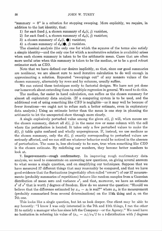
"summary = 0" is a criterion for stopping sweeping. More explicitly, we require, in
addition to the last identity, that:
1) for each fixed j, a chosen summary of dR{i, j) vanishes,
2) for each fixed i, a chosen summary of dB(i, j) vanishes;
3) a chosen summary of dIt (i, #) vanishes;
4) a chosen summary of dR{%, j) vanishes.
The classical analysis (the only one for which the squares of the terms also satisfy
a simple identity—and the only one for which a noniterative solution is available) arises
when each chosen summary is taken to be the arithmetic mean. Cases that are often
more useful arise when this summary is taken to be the median, or to be a good robust
estimator such as CXO.
Note that we have defined our desires implicitly, so that, since our good summaries
are nonlinear, we are almost sure to need iterative calculation to do well enough in
approximating a solution. Repeated "sweepings out" of any nonzero values of the
chosen summary, alternately by rows and by columns, usually suffice.
We can extend these techniques cosily to factorial designs. We have not yet done
our homework about extending them to multiple regression in general. We need to do this.
The median, far easier in hand calculation, can suffice as the chosen summary for
almost all exploratory data analysis. (If a computing system is to be used, and the
additional cost of using something like CXO is negligible—as it may well be because of
fewer iterations—-we ought not to refuse such a better estimate, even in exploratory
data analysis.) Using an estimate better than the mean is one step in planning the
arithmetic to let the unexpected show through more clearly.
A single explosively perturbed value among the given x(i, j) will, when means are
the chosen summary, distort all d(i, j) in the same row or same column with the cell
where the perturbation is located. It takes only a few perturbed values to make the
d(i, j) table quite confused and wholly unperspicuous. If, instead, we use medians as
the chosen summary, only the d(i, j) exactly corresponding to perturbed values are
seriously affected, and we can still see whatever behavior could be noticed in the absence
of perturbation. The same is, less obviously to be sure, true when something like CXO
is the chosen estimate. By redefining our numbers, they become better numbers to
look at.
7. Improvements—rough confirmatory. In improving rough confirmatory data
analysis, we need to concentrate on answering new questions, on giving several answers
to what seems a single question, and on simplifying our techniques. Suppose that we
have measured 37 different things that may reasonably be compared, and that we have
good evidence that the fluctuations (regrettably often called "errors") of our 37 measure-
ments (probably summaries of repetitions) behave like random samples from a Gaussian
distribution of mean zero and variance <r2, and that, moreover, we have an estimate
s2 of a2 that is worth / degrees of freedom. How do we answer the question: "Should we
believe that the difference estimated by xn — x7 is real?" where xn is the measurement
(probably summarized from several determinations) on the 11th thing and x7 on the
7th one.
This looks like a single question, but let us look deeper. One client may be able to
say honestly: "I know I was only interested in the 7th and 11th things, I ran the other
35 to satisfy a manager who has since left the Company—-or the Agency." We need have
no hesitation in referring his value of (a;u — x7)/s\/2 to a i-distribution with / degrees
DATA ANALYSIS, COMPUTATION AND MATHEMATICS 59
of freedom—or, as will usually be easier and more robust, using the analogous sign-test
procedure, either for significance or for confidence.
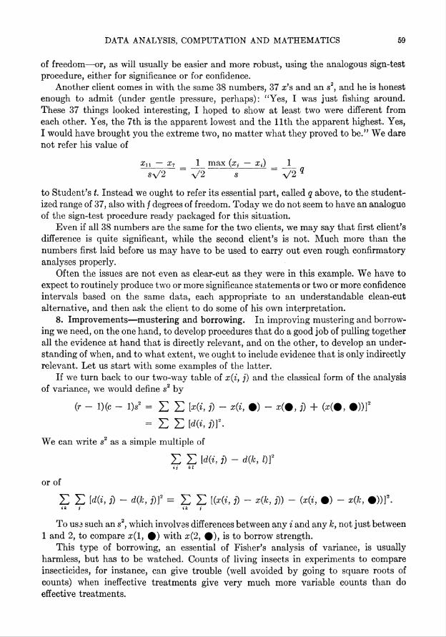
Another client comes in with the same 38 numbers, 37 x's and an s2, and he is honest
enough to admit (under gentle pressure, perhaps): "Yes, I was just fishing around.
These 37 things looked interesting, I hoped to show at least two were different from
each other. Yes, the 7th is the apparent lowest and the 11th the apparent highest. Yes,
I would have brought you the extreme two, no matter what they proved to be." We dare
not refer his value of
Zn — x7 1_ max (Xj — xt) 1_
sy/2 ~ V2 s ~ V2 Q
to Student's t. Instead we ought to refer its essential part, called q above, to the student-
ized range of 37, also with / degrees of freedom. Today we do not seem to have an analogue
of the sign-test procedure read}' packaged for this situation.
Even if all 38 numbers are the same for the two clients, we may say that first client's
difference is quite significant, while the second client's is not. Much more than the
numbers first laid before us may have to be used to carry out even rough confirmatory
analyses properly.
Often the issues are not even as clear-cut as they were in this example. We have to
expect to routinely produce two or more significance statements or two or more confidence
intervals based on the same data, each appropriate to an understandable clean-cut
alternative, and then ask the client to do some of his own interpretation.
8. Improvements—mustering and borrowing. In improving mustering and borrow-
ing we need, on the one hand, to develop procedures that do a good job of pulling together
all the evidence at hand that is directly relevant, and on the other, to develop an under-
standing of when, and to what extent, we ought to include evidence that is only indirectly
relevant. Let us start with some examples of the latter.
If we turn back to our two-way table of x(i, j) and the classical form of the analysis
of variance, we would define s2 by
(r - 1)(c l)s2 = £ £ M*, j) - x(i, ®) - *(#, j) + (*(#, #))]2
= £ £ W, ])]'■
We can write s2 as a simple multiple of
£ £ [d(i, j) - d(k, 0]2ii k I
or of
£ E W, j) - d(k, j)]2 -EE [(*(*', j) ~ X(k, ])) - (x(i, •) - x(k, #))]2.»k j ik i
To us3 such an s2, which involves differences between any i and any k, not just between
1 and 2, to compare x(l, #) with x(2, #), is to borrow strength.
This type of borrowing, an essential of Fisher's analysis of variance, is usually
harmless, but has to be watched. Counts of living insects in experiments to compare
insecticides, for instance, can give trouble (well avoided by going to square roots of
counts) when ineffective treatments give very much more variable counts than do
effective treatments.
60 JOHN W. TUKEY
A more interesting borrowing, requiring more care, arises when the j-index labels
states (like Iowa and Nebraska) and the x(i, #), directly relevant to averages over all
the states for which values are included, are used to give an answer for a single one of
these states. Now we borrow strength more vehemently. This is usually not overtly
advocated in the books. It is often done, however, and I would not want to say that
the net effect of doing it is bad. (I do think that doing it overtly rather than covertly
could lead to real gains.)
The art of borrowing enough, not too much—-and then making clear what you have
done—-is an important part of any data analyst's armamentarium, be he subject-matter
expert or professional data analyst.
Mustering strength is a more mundane—-one might almost dare to say more mathe-
matical—-matter. We have already looked briefly at the simplest paradigm—-summari-
zation of location for a batch—to which we shall return. What has been learned in that
simple case needs now to be expanded to cover many more complex situations.
Some would like to say "But you are leaving no place for the theory of sampling
from exactly Gaussian distributions!" I understand the feeling, but cannot agree with
the conclusion. Sometimes, when a road is being rebuilt—or built for the first time—-the
builders will drive wooden piles as cribwork for a temporary bridge, whose abutments
are unsettled fill, paved with unsupported macadam. Traffic is only to use such a detour
until the concrete bridge, the well-settled abutments, and the well-supported permanent
road surface are ready for use. Gaussian sampling theory is like the temporary bridge,
very useful, but. . . . It is high time that we complete and put to use many more solid
concrete bridges.
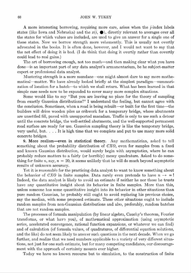
9. More realism—even in statistical theory. Any mathematician, asked to tell
something about the probability distribution of CXO, even for samples from a fixed
and known Gaussian distribution, would surely begin with asymptotics, where he can
probably reduce matters to a fairly (or horribly) messy quadrature. Asked to do some-
thing for finite n, say, n = 20, it seems unlikely that he will do much beyond asymptotic
results of unknown accuracy.
Yet it is reasonable for the practicing data analyst to want to know something about
the behavior of CXO in finite samples. Data rarely even pretends to have n co !
Indeed, the data analyst is likely to avoid an estimate if neither he nor those he trusts
have any quantitative insight about its behavior in finite samples. More than this,
unless someone has some quantitative insight into its behavior in other situations than
pure random Gaussian, he probably still ought to avoid replacing his previous choice,
say the median, with some proposed estimate. These other situations ought to include
random samples from non-Gaussian distributions and also, preferably, random batches
that are not random samples.
The processes of formula manipulation (by linear algebra, Cauchy's theorem, Fourier
transforms, or what hav3 you), of mathematical approximation (using asymptotic
series, accelerated convergence, rational function expansions, or whatever we can find)
and of calculation (of formula values, of quadratures, of differential equation solutions,
and the like) do not seem likely to answer such questions in the next decade. When we go
further, and realize that we need numbers applicable to a variety of very different situa-
tions, not just for one such estimate, but for many competing candidates, our discourage-
ment with the approach of certainty mounts ever higher.
Today we have no known recourse but to simulation, to the construction of finite
DATA ANALYSIS, COMPUTATION AND MATHEMATICS 61
structures as an approximation to the possible samples and probabilities of our prob-
ability models. The naive approach is raw experimental sampling—-naive and so costly
as often to be quite unfeasible. Economics dictates that we turn to the mathematically
sound "swindles" of Monte Carlo, to modifications of the probability problem that can
be mathematically shown to give the same answer in the limit as the problem that we
have fixed upon, and that do, in practice, approach the common limit much faster.
In the Buffon needle problem, for example, we can replace a short needle by a large,
nearly regular n-gon, the length of each of whose sides is an integer multiple of the length
of the needle. The arithmetic mean number of line crossings for the n-gon has only to be
divided by the n-gon's perimeter in needle lengths to approach much more rapidly the
same limit as the arithmetic mean number of short needle crossings. (Compare [9], [6], [12].)
There is merit in reasonably close approximation of the results of each of our actual
simulations to the results corresponding to the mathematical model whose name we
associate with that simulation. There is no merit in unreasonably close agreement.
Once the agreement is to a small fraction of the difference between mathematical models
that are plausible alternatives for approximating the real world, closer approximation
is almost worthless.
In the study already referred to [1] a Monte Carlo investigation of first 40 and then 65
estimates—-most of about the general complexity of 215 and C02—was carried out for
a variety of situations, eventually 37 in number. A further study now in progress [11]
is looking at a new set of 75 estimates. These studies also look at a few linear combina-
tions of each pair of the basic estimates. For the second 75, which can be expanded to 111
because of certain properties of sit means, there will be §(112)(111) = 6216 estimates
of the complexity of CXO, namely "J of one plus § another" (where both may be the
same). It is hard to estimate how soon the approach of certainty might be able to replace
the approach of simulation here.
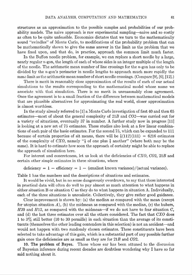
For interest and concreteness, let us look at the deficiencies of CXO, C02, 21B and
certain other simple estimates in three situations, where
deficiency = 1 — efficiency = 1 — (smallest known variance)/(actual variance).
Table 1 has the numbers and the descriptions of situations and estimates.
It would be vivid, but in no sense dangerously overdrawn, to say that those interested
in practical data will often do well to pay almost as much attention to what happens in
either situation B or situation C as they do to what happens in situation A. Individually,
each of the three situations is unrealistic. Collectively, they give rather good guidance.
Clear improvement is shown by: (a) the median as compared with the mean (except
for Utopian situation A), (b) the midmean as compared with the median, (c) the hubers,
#20 and H12, as compared with the midmean—if we do not have to fear situation C,
and (d) the last three estimates over all the others considered. The fact that CXO does
1 to 3% still better (10 to 30 permille) in each situation than the average of its consti-
tuents (themselves the other leading contenders in this selection) is not an accident—-and
would not happen with two randomly chosen estimates. These constituents have been
selected to take advantage of this gain, which is a substantial part of any possible further
gain once the deficiencies are as small as they are for 21B and C02.
10. The problem of Bayes. Those whose ear has been attuned to the discussion
of Bayesian inference during recent decades are doubtless wondering why I have so far
said nothing about it.
62 JOHN W. TUKEY
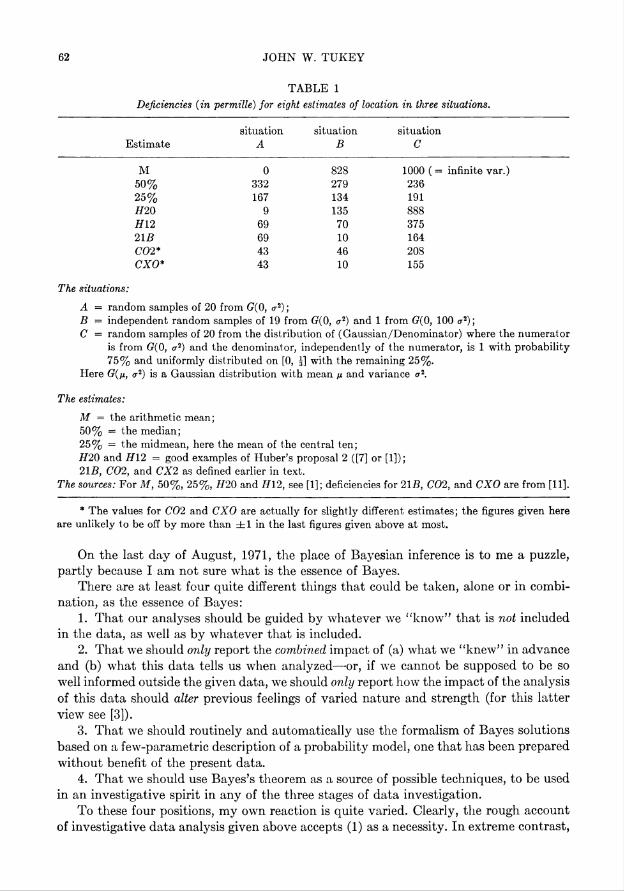
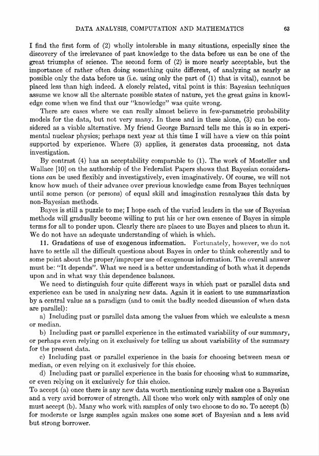
TABLE 1
Deficiencies (in permille) for eight estimates of location in three situations.
situation situation situation
Estimate ABC
M 0 828 1000 (= infinite var.)
50% 332 279 23625% 167 134 191H20 9 135 888#12 69 70 375215 69 10 164
C02* 43 46 208CXO* 43 10 155
The situations:
A = random samples of 20 from (7(0, <rJ);
B — independent random samples of 19 from (?(0, <r2) and 1 from G(0, 100 o-2);
C = random samples of 20 from the distribution of (Gaussian/Denominator) where the numerator
is from 0(0, <r2) and the denominator, independently of the numerator, is 1 with probability
75% and uniformly distributed on [0, j] with the remaining 25%.
Here (7(/x, <r2) is a Gaussian distribution with mean /i and variance o-2.
The estimates:
M = the arithmetic mean;
50% = the median;
25% = the midmean, here the mean of the central ten;
H20 and H12 = good examples of Huber's proposal 2 ([7] or [1]);
21-B, C02, and CX2 as defined earlier in text.
The sources: For M, 50%, 25%, H20 and H\2, see [1]; deficiencies for 21B, C02, and CXO are from [11].
* The values for C02 and CXO are actually for slightly different estimates; the figures given here
are unlikely to be off by more than ±1 in the last figures given above at most.
On the last day of August, 1971, the place of Bayesian inference is to me a puzzle,
partly because I am not sure what is the essence of Bayes.
There are at least four quite different things that could be taken, alone or in combi-
nation, as the essence of Bayes:
1. That our analyses should be guided by whatever we "know" that is not included
in the data, as well as by whatever that is included.
2. That we should only report the combined impact of (a) what we "knew" in advance
and (b) what this data tells us when analyzed—-or, if we cannot be supposed to be so
well informed outside the given data, we should only report how the impact of the analysis
of this data should alter previous feelings of varied nature and strength (for this latter
view see [3]).
3. That we should routinely and automatically use the formalism of Bayes solutions
based on a few-parametric description of a probability model, one that has been prepared
without benefit of the present data.
4. That we should use Bayes's theorem as a source of possible techniques, to be used
in an investigative spirit in any of the three stages of data investigation.
To these four positions, my own reaction is quite varied. Clearly, the rough account
of investigative data analysis given above accepts (1) as a necessity. In extreme contrast,
DATA ANALYSIS, COMPUTATION AND MATHEMATICS 63
I find the first form of (2) wholly intolerable in many situations, especially since the
discovery of the irrelevance of past knowledge to the data before us can be one of the
great triumphs of science. The second form of (2) is more nearly acceptable, but the
importance of rather often doing something quite different, of analyzing as nearly as
possible only the data before us (i.e. using only the part of (1) that is vital), cannot be
placed less than high indeed. A closely related, vital point is this: Bayesian techniques
assume we know all the alternate possible states of nature, yet the great gains in knowl-
edge come when we find that our "knowledge" was quite wrong.
There are cases where we can really almost believe in few-parametric probability
models for the data, but not very many. In these and in these alone, (3) can be con-
sidered as a viable alternative. My friend George Barnard tells me this is so in experi-
mental nuclear physics; perhaps next year at this time I will have a view on this point
supported by experience. Where (3) applies, it generates data processing, not data
investigation.
By contrast (4) has an acceptability comparable to (1). The work of Mosteller and
Wallace [10] on the authorship of the Federalist Papers shows that Bayesian considera-
tions can be used flexibly and investigatively, even imaginatively. Of course, we will not
know how much of their advance over previous knowledge came from Bayes techniques
until some person (or persons) of equal skill and imagination reanalyzes this data by
non-Bayesian methods.
Bayes is still a puzzle to me; I hope each of the varied leaders in the use of Bayesian
methods will gradually become willing to put his or her own essence of Bayes in simple
terms for all to ponder upon. Clearly there are places to use Bayes and places to shun it.
We do not have an adequate understanding of which is which.
11. Gradations of use of exogenous information. Fortunately, however, we do not
have to settle all the difficult questions about Bayes in order to think coherently and to
some point about the proper/improper use of exogenous information. The overall answer
must be: "It depends". What we need is a better understanding of both what it depends
upon and in what way this dependence balances.
We need to distinguish four quite different ways in which past or parallel data and
experience can be used in analyzing new data. Again it is easiest to use summarization
by a central value as a paradigm (and to omit the badly needed discussion of when data
are parallel):
a) Including past or parallel data among the values from which we calculate a mean
or median.
b) Including past or parallel experience in the estimated variability of our summary,
or perhaps even relying on it exclusively for telling us about variability of the summary
for the present data.
c) Including past or parallel experience in the basis for choosing between mean or
median, or even relying on it exclusively for this choice.
d) Including past or parallel experience in the basis for choosing what to summarize,
or even relying on it exclusively for this choice.
To accept (a) once there is any new data worth mentioning surely makes one a Bayesian
and a very avid borrower of strength. All those who work only with samples of only one
must accept (b). Many who work with samples of only two choose to do so. To accept (b)
for moderate or large samples again makes one some sort of Bayesian and a less avid
but strong borrower.
64 JOHN W. TUKEY
Many accept (c) without hesitation, no matter what the size of the present body
of data. For smaller bodies of data, what else could be done? To do this for quite large
bodies of data—a thousand observations or more, perhaps—is to take a very Bayes-like
position, often without thought or recognition.
To accept (d), unless the new data is much more than all past data combined (as
happened on 1 May 1960 for data about the interior structure of the earth), is to practice
science as the best scientists do it.
As we have seen, the amount of data does, and should, shift the attitude we take up
and down this scale. As we have seen, there are many intervening choices between ex-
treme un-Bayes and extreme Bayes. Which choices are reasonably wise will vary from one
set of circumstances to another. What we need is better guidance for our choosing.
12. Close. We have now had a short conducted tour through some of the attitudes,
approaches, and problems of data analysis. We have stressed the investigative and
theoretical aspects, because I believe you all accept the routine processing of data as a
matter for computing-system arithmetic and not a matter of finding new formulas by
formula manipulation.
If anyone, here or later, can tell us how the approach of certainty—traditional mathe-
matics—is going to answer the questions that practical data analysts are going to have
to have answered, I will rejoice. Such a route will surely be easier and cheaper, and there
will be many more ready to follow it up at once with effective work.
But until I am reliably informed of such a Utopian prospect, I shall expect the
critical practical answers of the next decade or so to come from the approach of simula-
tion—from a statistician's form of mathematics, in which ever more powerful computing
systems will be an essential partner and effective, mathematically sound "swindles"
will be of the essence.
To take this view does nothing to discount the paraphrase made by the late great
John von Neumann: "The only good Monte Carlo is a dead Monte Carlo!" This aphorism
was coined to express the view that out of a well-conducted Monte Carlo should come
enough insight to allow us to use newly-developed or newly-chosen approximations to
solve other cases of that particular complexity, thus needing to use Monte Carlo again
only when we want to go still further or still deeper. I approve this goal; I only wish I
could reach it more often.
References
[1] D. F. Andrews, P. J. Bickel, F. R. Hampel, P. J. Huber, W. H. Rogers and J. W. Tukey, Robust
estimates of location: survey and advances, Princeton University Press, 1972
[2] F. J. Anscombe, Topics in the investigation of linear relations fitted by the melhod of least squares,
J. Roy. Stat. Soc. B29, 1-29 and 49-52 (1967), especially page 3, footnote
[3] J. M. Dickey, Bayesian alternatives to the F-test, presented at the joint statistical meetings, Ft.
Collins, Colorado, 26 August 1971 (Also: Research Report No. 50, Statistics Department, State
University of New York at Buffalo, Revised version, August, 1971)
[4] Churchill Eisenhart, The development of the concept of the best mean of a set of measurements from
antiquity to the present day, Presidential address to the American Statistical Association, Ft. Collins,
Colorado, 24 August 1971[5] J. C. Gower and G. J. S. Ross, Minimum spanning trees and single linkage cluster analysis, Appl.
Stat. 18, 54-64 (1969)[6] J. C. Hammersley and K. W. Morton, A new Monte Carlo technique: antithetic variales, Proc. Camb.
Phil. Soc. 52, 449-475 (1956)[7] P. J. Huber, Robust estimation of a location parameter, Ann. Math. Statistics 35, 73-101 (1964);
see proposal 2 on page 96

DATA ANALYSIS, COMPUTATION AND MATHEMATICS 65
[8] Rudyard Kipling, Soldiers Three and Military Tales, Part 1, in The works of Rudyard Kipling,
volume 2, Charles Scribner's Sons, New York, 1897; see page 159
[9] N. Mantel, An extension of the Buff on needle -problem, Ann. Math. Statistics 24, 624-677 (1954)
[10] Frederick Mosteller and D. L. Wallace, Inference and disputed authorship: The Federalist, Addison-
Wesley, Reading, Mass. 1964
[11] W. H. Rogers and J. W. Tukey, in preparation
[12] J. W. Tukey, Antithesis or regressionf Proc. Camb. Phil. Soc. 53, 923-924 (1957)
[13] J. W. Tukey, Exploratory data analysis, three volumes, limited preliminary edition, Addison-
Wesley, Reading, Mass., 1970-71; see first page of preface
[14] J. W. Tukey, Lags in statistical technology, presented at the first Canadian Conference on Applied
Statistics, June 2, 1971; to appear in the Proceedings of that Conference, 1972
Recommended
![COMP 333 Data Analytics [2ex] Exploratory Data Analysisusers.encs.concordia.ca/~gregb/home/PDF/comp333-eda.pdf · Exploratory Data Analysis Tukey 1977 book John Tukey (1977), Exploratory](https://img.pdfslide.us/doc/110x75/6014a0de4bad7c5bfa790925/comp-333-data-analytics-2ex-exploratory-data-gregbhomepdfcomp333-edapdf.jpg)