ASYMPTOTIC ANALYSIS AND COMPUTATION FOR SHELLS

by Charles R. Steele

Applied Mechanics Division Stanford University Stanford, CA 94305

ABSTRACT Several examples are discussed of asymptotic results illustrating key features of thin shell behavior and possibly extending the benchmark problems for verification of direct numerical procedures. The basic nature of shell solutions for static loading usually can be categorized as membrane, inextensional, and edge effect. With different boundary conditions or geometry, different solution types dominate, with results for the stress and displacement in the shell differing by orders of magnitude. Approximate results for the nonlinear, large displacement of a spherical shell are shown for point, line, and moment loading, obtained by using an "inverted dimple" and edge effect solutions. Results for the maximum bending and maximum direct stress under a nearly concentrated load are included, which demonstrate the transition from slowly varying behavior to the point load with logarithmic singularity for shells of positive, negative, and zero curvature. It is suggested that a minimum condition for a

proper shell element is that all such behavi

or be represented. 1. INTRODUCTION The analysis of shells always presents a challenge because of difficulties in formulating of the equations and computing solutions. The latter arise because a small parameter, the thickness-to-radius ratio, multiplies the high derivative terms, giving a "stiff" system of equations. For such equations, perturbation or asymptotic methods are successful for a number of special cases and are the basis for the standard design formulas used for many years. Because of various restrictions on such formulas, it is important to have general numerical solution methods, such as those offered by finite element analysis. To ascertain the accuracy of the finite element calculations, a few benchmark problems typically have been used. These problems are good in themselves, but do not properly cover the range of behavior of thin shells. Therefore, in this paper problems are selected to expand the range of benchmark problems and clarify the behavior which can be expected from a shell in different situations. Volumes have been written on the latter aspect, which are hardly represented within the limitations of this paper. Nevertheless there may be some value in this summary of some key features and specific numerical values.

Only the static behavior of the isotropic shell is

touched upon. In each area such as dynamic response,

composites, and fluid-shell interaction, there are

many additional interesting features.

2. GENERAL CHARACTERISTICS OF THIN-SHELL SOLUTIONS

As indicated in the lecture by Calladine (Ref. 5),

understanding the fundamental behavior of shells did

not come easily, and involved substantial differences

in opinion among eminent workers in mechanics such as

Love, Lamb, and Rayleigh. These differences were

resolved, to a considerable extent, in the 1927

publication of the classic work on elasticity by Love

(Ref. 17). Most concepts in this paper can be found

at least implicitly in that edition. Later works by

Flügge (Ref. 10), Gol'denweiser (Ref. 12), Reissner

(Ref. 26), Vlasov (Ref. 39), and Timoshenko and

Woinowsky-Kreiger (Ref. 38) greatly extended the

knowledge, and the process continues with the more

recent works of Axelrad (Ref. 2), Bushnell (Ref. 3),

Calladine (Ref. 4), Donnell (Ref. 6), Dowell (Ref. 7),

Dym (Ref. 8), Gibson (Ref. 11), Gould (Ref. 13),

Kraus (Ref. 15), Niordson (Ref. 21), Seide (Ref. 30),

and many others. There is a tendency for this

information to be overlooked, with the notion that a

proper finite element and enough computing power are

adequate to tame any structural system. In fact, the

thin shell places a severe demand on both element

architecture and computing resources. Some reasons

for this are evident in the basic behavior of the

shell solutions.

A curious feature is that generally correct

behavior of shell solutions was understood long before

a satisfactory basic theory was obtained. A

comprehensive treatment of the subject is given by

Naghdi (Ref. 20)

For minimal notational complexity, we consider the

linear, elastic solution for the shell of revolution,

and use a Fourier series in the circumferential angle

q. Because for each harmonic the equations form an

eighth order system of ordinary differential

equations, the normal displacement component w for

the one harmonic can be written as:

w ( s, θ ) = wn (s ) cos nθ = ∑

j = 1

9

Cj wjn ( s ) cos nθ

(1)

in which s is the meridional arc length, and the

coefficient C9 = 1 multiplies the particular solution

for nonzero surface loads. The remaining constants

are the constants of integration which must be

determined from the boundary conditions. A dominant

parameter for the response of shells is:

λ = r2 / c 1/2 (2)

where c is the reduced thickness t, and the

representative size of the shell is taken as the

normal radius of circumferential curvature r2:

c = t / 12 ( 1 - v 2 ) 1/2 R = r2 = r

sin φ (3)

Unlike beam, plane stress, plain strain, or three-

dimensional solid problems, the order of magnitude of

the constants depends very much on the type of

boundary conditions which are applied to the thin

shell. The cause is the drastically different

behavior of the different solutions wj (s). Two of

these (say for j = 1,2) are "membrane" solutions, for

which the significant stress is "direct", i.e., the

average tangential stress through the thickness. The

relative magnitude of the displacement and stress

quantities is shown in the first column of Table 1,

taken from Steele (Ref. 33). This type of solution is

sometimes referred to as "momentless"; however, keep

in mind that bending and transverse shear stresses are

usually present, but at a reduced magnitude. The

second type of solution (say for j = 3,4) is

"inextensional bending", for which the midsurface

strains are nearly zero. This is indicated in the

second column in Table 1. The direct stress of the

membrane solution and the curvature change of the

inextensional solution satisfy the same equation, so

these have similar variation over the surface.

Specifically these are "slowly varying". As indicated

by the first two rows in Table 1, taking the

derivative of the displacement, or any other quantity,

does not increase the order of magnitude. Thus the

inextensional solution is similar to the membrane

solution for displacement, bending stress and

transverse shear, but has direct stress reduced by

four orders of magnitude. The third type of solution

is referred to as "edge effect" because it is

characterized by exponential decay in magnitude with

the distance from a boundary. The distance in which

the solution decreases to about 4 percent of the edge

magnitude is:

δ = π 2 r2 c 1/2 ≈ 2.5 r2 t 1/2 = O ( R / λ ) (4)

The relative magnitudes of stress and displacement are

indicated by the third column in Table 1. The

particular solution for a smooth distribution of

surface load (j =9) is generally similar to the

membrane solution.

An anomaly of thin shell behavior is that the

load can be carried efficiently over a broad expanse

by the membrane solution. However, peak stress occurs

in the narrow edge zone, which often is the site of

failure initiation. To capture properly the edge

effect with finite elements using polynomials of low

order, a mesh spacing no greater than about d / 10

must be used. For static problems, the elements can

be kept to a reasonable number by using a fine mesh

near the boundaries and a course mesh elsewhere. For

problems of vibration and wave propagation,

significant bending waves occur everywhere in the

shell which have the wave length of the order of

magnitude of d. A proper solution requires a fine

mesh of elements everywhere. Nonlinear material and

geometric behavior can be significant in distances

small in comparison with d, requiring even a finer

mesh of elements.

The preceding discussion concerns the relative

sizes of the components in a single column of Table 1.

The total solution is the sum of the three columns,

for which the relative magnitudes between columns is

important. This depends strongly on the type of

boundary conditions prescribed for the shell.

2.1 Displacement Boundary Conditions

The edge effect makes a small contribution to the

meridional and circumferential components of

displacement; thus, the four constants of the membrane

and inextensional solutions are used to satisfy these

conditions with constants O(1). The edge effect

solutions then are used to satisfy the conditions on

the normal displacement and rotation, also with

constants O(1). Thus, the contribution of each type

of solution to the normal component of displacement

is the same order of magnitude, producing the relative

magnitudes both within each column and between the

first three columns of Table 1. An important

conclusion is that the edge effect stress is the same

order of magnitude as the interior membrane solution.

The bending stress of the inextensional solution is

negligible. In this situation, the shell is a very

efficient structure for spanning space and carrying

load.

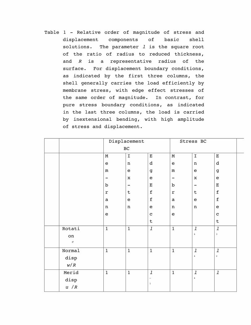
Table 1 - Relative order of magnitude of stress and

displacement components of basic shell

solutions. The parameter l is the square root

of the ratio of radius to reduced thickness,

and R is a representative radius of the

surface. For displacement boundary conditions,

as indicated by the first three columns, the

shell generally carries the load efficiently by

membrane stress, with edge effect stresses of

the same order of magnitude. In contrast, for

pure stress boundary conditions, as indicated

in the last three columns, the load is carried

by inextensional bending, with high amplitude

of stress and displacement.

Displacement

BC

Stress BC

M

e

m

-

b

r

a

n

e

I

n

e

x

-

t

e

n

E

d

g

e

E

f

f

e

c

t

M

e

m

-

b

r

a

n

e

I

n

e

x

-

t

e

n

E

d

g

e

E

f

f

e

c

t

Rotati

on

c

1 1 l 1 l4

l3

Normal

disp

w/R

1 1 1 1 l4

l2

Merid

disp

u /R

1 1 l–

1

1 l4

l

Circum

disp

v /R

1 1 l–

2

1 l4

1

Merid

stress

Ns /Et

1 l–

4

l–

1

*

1 1 l

*

Circum

stress

Nq /Et

1 l–

4

1 1 1 l2

Shear

stress

Nsq /Et

1 l–

4

l–

1

*

1 1 l

*

Merid

bendin

g

stress

Ms /Et 2

l–

2

l–

2

1 l–

2

l2

l2

Transv

erse

shear

stress

Qs /Et

l–

4

l–

4

l–

1

*

l–

4

1 l

*

* Denotes items linearly dependent in the

leading terms

2.2 Stress Boundary Conditions

For prescribed stresses on the boundaries of

beams, plates, and three-dimensional solids, the

stress boundary value problem is just the inverse of

the displacement problem, with the same order of

magnitude of stress and displacement. This is

definitely not the case for the thin shell, for which

the matrix for computing the constants of integration

is nearly singular. This can be understood if one

attempts the same reasoning as used before for

prescribed displacement, using the first three columns

of Table 1. With all constants the same order of

magnitude, the inextensional and edge effect provide

small contribution to the meridional and shear stress.

However, the membrane solution does not have enough

constants to satisfy both stress components at the two

edges. Consequently, the constants of integration

cannot have the same order of magnitude. Because of

the linear dependence of components in the edge

effect, the result is that the constants of the

inextensional and edge effect solutions must be large

(C3, C4 = O(l 4 ), C5– C8 = O(l 2 )), producing the

magnitudes shown in the last three columns of Table 1.

The total state of stress and displacement is

dominated by the inextensional solution. The

difference in boundary conditions is summarized by the

following: prescribed displacements O(1) produce

stress O(1); prescribed edge stress O(1) produces

displacements of order O(l 4 ) and interior bending

stress O(l 2). This is why the simple inextensional

solution of Rayleigh for the first modes of vibration

of a hemisphere is quite accurate. Also quite

accurate (if the shell is not too long) is the

solution in Timoshenko and Woinowsky-Kreiger (Ref.

38) for the cylinder with free ends and loaded by

pinch concentrated forces in the center. The

asymptotic results for all edge stiffness and the

inverse flexibility coefficients for shells of

positive, negative and zero curvature are given by

Steele (Ref. 34). From these, it is easy to see that

the inextensional solutions for a pinch load will be

accurate for the displacement because of rapid

convergence of the Fourier series solution. The

Fourier series representation is not convergent for

the stress, because the stress under a point load has

a logarithmic singularity.

Another interpretation of the behavior is that the

properly stiffened shell has stress and displacement

similar to that in plane stress or axial loading of a

straight bar (stiffness = Et ), while the shell with

free edges has stress and displacement similar to that

of transverse bending of a beam or plate (stiffness =

Etc 2 = E t O(l 4 )).

Note that in the inextensional solution the direct

stress resultant tensor is not symmetric; however,

the direct stress is virtually negligible compared to

the bending stress.

2.3 Mixed Boundary Conditions

For mixed boundary conditions various

possibilities exist for combinations of the behavior

discussed in the preceding two sections. The simple

rule of thumb is that if the tangential displacement

conditions permit an inextensional solution, this

will, indeed, dominate the total solution. As

discussed in many of the references cited, the details

depend strongly on the Gaussian curvature of the

shell, because the equations for the membrane and

inextensional behavior are elliptic, parabolic and

hyperbolic for surfaces which are elliptic, parabolic

and hyperbolic, respectively.

3. AXISYMMETRIC LOADING EXAMPLES

For the static, axisymmetric deformation of a

shell of revolution, as well as for the first

nonaxisymmetric harmonic cosq, the problem simplifies

considerably, because the inextensional solution

consists of rigid body displacements. Thus, only

columns 1 and 3 in Table 1 are of concern. The

membrane solution is often obtained by simple static

equilibrium considerations, while the most relevant

information on the edge effect is the knowledge of the

decay distance (Eq. 4) and the relation between the

edge stress and displacement quantities, i.e., the

edge stiffness coefficients.

χ , M s

H, h

r

z

φ

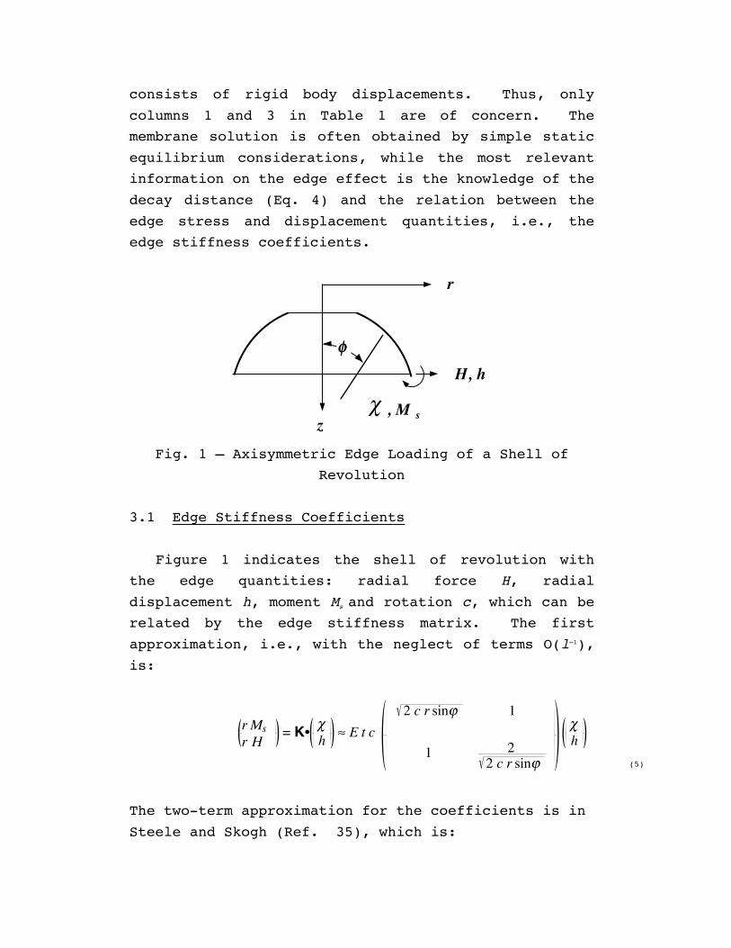
Fig. 1 – Axisymmetric Edge Loading of a Shell of

Revolution

3.1 Edge Stiffness Coefficients

Figure 1 indicates the shell of revolution with

the edge quantities: radial force H, radial

displacement h, moment Ms and rotation c, which can be

related by the edge stiffness matrix. The first

approximation, i.e., with the neglect of terms O(l–1),

is:

r Ms r H

= K• χh ≈ E t c

2 c r sinϕ 1

1 22 c r sinϕ

χh

(5)

The two-term approximation for the coefficients is in

Steele and Skogh (Ref. 35), which is:

k11 = E t c 2 c r sinϕ 1 + ν cotϕ 2 c r2

1 2 + O λ –2

k12 = k21 = E t c 1 + 14

+ r2

4 r1

+ ν cotϕ 2 c r2

1 2 + O λ –2 (6)

k22 = k12 22 c r sinϕ

1 + O λ –2

in which r1 is the meridional radius of curvature and

r2 = r / sin f. These approximations are accurate

when the correction term in brackets is less than

about 0.2, which covers a wide range of shell

geometry, but excludes the vicinity of the apex of

toroid and sphere, where sin f = 0. Of interest is

that the first term depends only on the meridional

slope at the edge, while the correction terms bring in

the effect of the meridional curvature.

The effect of transverse shear deformation and

membrane prestress can be added:

k11 = k11 6 f f + ρ + β /2

f + β

k12 = k12 6 1f + β

(7)

k22 = k22 6

f + ρ + β /2

f + β

f = 1 + 2 ρ β

The subscript 6 denotes the expressions in Eq. 6, the

prestress factor is:

ρ = Ns r2

2 E t c (8)

and the transverse shear factor is:

β = E c

Gt r2 (9)

in which Gt is the equivalent transverse shear

modulus. For a thick shell or a composite with a

relatively soft matrix, b is significant.

When the meridional membrane stress increases in

tension, r becomes more positive and the stiffness

coefficients increase in magnitude. For compression,

the stiffness approaches zero as the critical value is

approached:

ρcr = – 1 – β / 2 (10)

Eq. 10 provides the "classical" buckling load. The

inverse matrix of flexibility coefficients has a

singularity when r approaches the value which is half

of Eq. 10. Thus the free edge has an instability at

one-half of classical buckling load, as pointed out by

Hoff and Soong (Ref. 14) for the cylindrical shell.

The first geometric nonlinearities can be obtained

from the Reissner equations for moderate rotation

theory. Results for the edge coefficients are in

Ranjan and Steele (Ref. 25). As an example, the term

providing the edge moment for a prescribed rotation

with the radial displacement fixed, has the

approximation:

k11 = k11 6

1 – 3 χ10 cot φ

(11)

This nonlinearity is of the softening type.

3.2 Pressure Vessel With Clamped Edge

Certainly, an important shell structure is the

pressure vessel. Despite the fact that the shell

generally carries the load by membrane action, the

maximum stress concentration occurs at the attachments

with stiffeners. Because these points are often the

site for failure initiation, it would seem that a

first requirement is the proper computation of such a

region. For example, the rigidly clamped edges in

Fig. 2 are considered. The membrane solution is well

known. To this the edge effect must be added, which

must have radial displacement and rotation which

cancel those of the membrane solution. Thus Eq. 5

readily gives the simplest, one-term approximation for

the edge meridional bending stress:

σsB = 6 Ms

t2 ≈ σsD 3

1 - ν2 1/2 2 – r2r1

– ν (12)

in which the reference meridional membrane (direct)

stress is the familiar value:

σsD = p r2

2 t (13)

and the error is given by the correction terms in Eq.

6. Thus, for n = 0.3, Eq. 12 gives the bending

stress factors:

σsB ≈ σsD × 1.27 spherical cap

3.10 cylinder (14)

which is a specific demonstration of the O(1) edge

effect in Table 1, column 3.

p

p

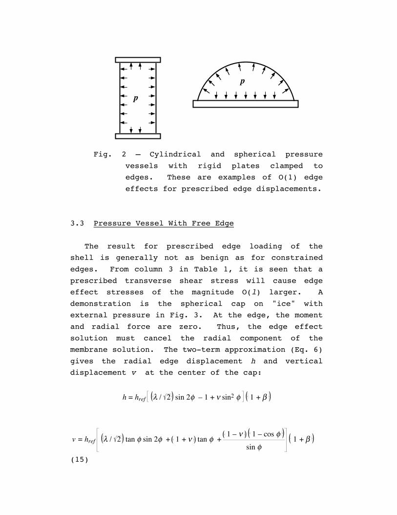
Fig. 2 – Cylindrical and spherical pressure

vessels with rigid plates clamped to

edges. These are examples of O(1) edge

effects for prescribed edge displacements.

3.3 Pressure Vessel With Free Edge

The result for prescribed edge loading of the

shell is generally not as benign as for constrained

edges. From column 3 in Table 1, it is seen that a

prescribed transverse shear stress will cause edge

effect stresses of the magnitude O(l) larger. A

demonstration is the spherical cap on "ice" with

external pressure in Fig. 3. At the edge, the moment

and radial force are zero. Thus, the edge effect

solution must cancel the radial component of the

membrane solution. The two-term approximation (Eq. 6)

gives the radial edge displacement h and vertical

displacement v at the center of the cap:

h = href λ / 2 sin 2φ – 1 + ν sin2 φ 1 + β

v = href λ / 2 tan φ sin 2φ + 1 + ν tan φ + 1 – ν 1 – cos φ

sin φ 1 + β

(15)

href = p R 2 sin φ2 E t

in which f is the angle at the edge. Specific

results are in Table 2 for a fixed edge angle. Fig. 3

demonstrates the distribution of stress and

displacement for R / t = 100. The one-term asymptotic

results in Table 2 are computed from the leading term

O(l ) in Eq. 15, while the two-term results are

computed from all terms in Eq. 15, including the

transverse shear deformation term for an isotropic

material. A comparison of the stress factor for the

constrained edge (Eq. 14) with Table 2 indicates the

penalty paid for inadequate stiffening of a shell.

Results from FAST1 are also in Table 2. This is a

prototype computer program combining asymptotic and

numerical methods. In the solution algorithm, if an

error condition is satisfied, the asymptotic solution

is used directly, with some direct numerical

integration. Otherwise, the shell is divided into

sections in which a power series solution is used.

For the R /t = 10 results in Table 2, the FAST1

program is using primarily the power series.

3.4 Pressure Vessel With Slope Discontinuity

The same behavior as in Fig. 3 occurs in a shell

with a discontinuity in the meridional slope. Such a

discontinuity causes a discontinuity in the radial

force resultant of the membrane solution. Thus, the

edge effect solutions must have a radial force

discontinuity of the opposite sign and same magnitude.

Again from Table 1, column 3, it is seen that this

produces the displacement and stress

Table 2 – Radial and vertical displacements for

spherical cap with external pressure and

without radial or moment constraint at the edge

f = p /4. The one- and two-term asymptotic

results and the calculation with FAST1 are

shown. The reference displacement is the

membrane displacement (with n = 0). The stress

concentration factors are similar in magnitude

to these displacement factors.

R /

t

Dis

p

1 -

ter

m

2-

ter

m

FAS

T1

10 h /

href

4.0

5

4.0

3

3.4

0

v /

href

4.0

5

7.0

2

7.2

5

100 v /

href

12.

8

12.

3

11.

9

h /

href

12.

8

14.

7

15.

3

100

0

v /

href

40.

5

39.

7

39.

5

h /

href

40.

5

42.

2

44.

5

0 3 6 x106

3

0

-3x10

Axia

l Dis

tanc

e Undeformed

Deformed

0 3 6 x10-1

0

1x10 4

Meridional Arclength s

SsOD

SsID

SthOD

SthID

Radial Distance

Stre

ss D

istri

butio

n

δ

p

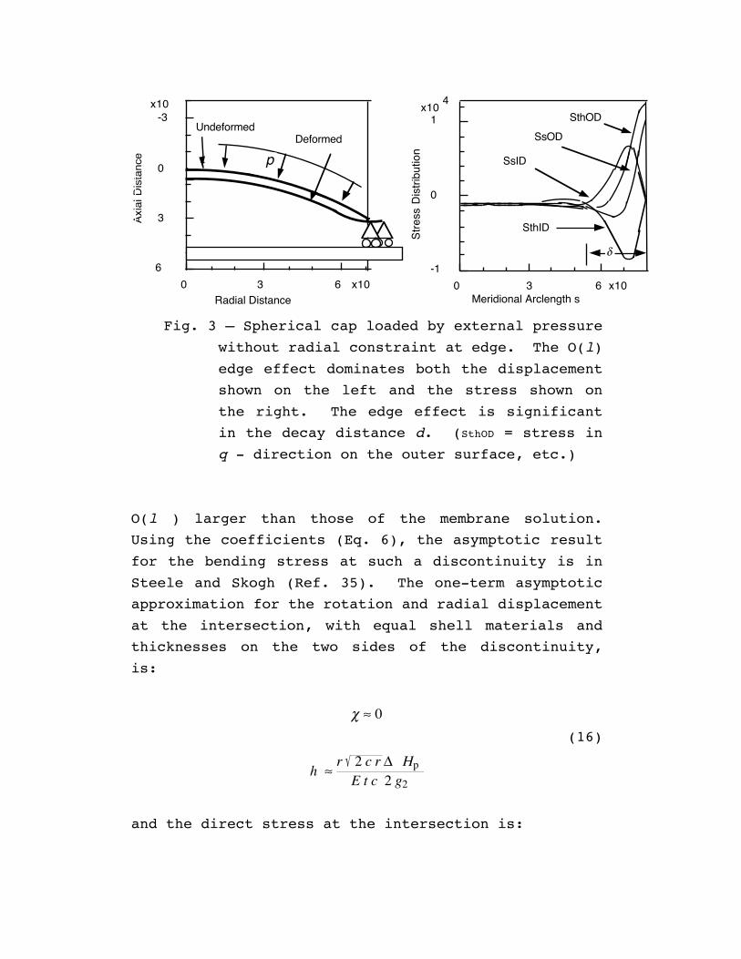
Fig. 3 – Spherical cap loaded by external pressure

without radial constraint at edge. The O(l)

edge effect dominates both the displacement

shown on the left and the stress shown on

the right. The edge effect is significant

in the decay distance d. (SthOD = stress in

q - direction on the outer surface, etc.)

O(l ) larger than those of the membrane solution.

Using the coefficients (Eq. 6), the asymptotic result

for the bending stress at such a discontinuity is in

Steele and Skogh (Ref. 35). The one-term asymptotic

approximation for the rotation and radial displacement

at the intersection, with equal shell materials and

thicknesses on the two sides of the discontinuity,

is:

χ ≈ 0 (16)

h ≈ r 2 c r Δ Hp

E t c 2 g2

and the direct stress at the intersection is:

σθ D = Nθ

t ≈ 1

g2 r

2 c Δ Hp

t (17a)

while the bending stress at the intersection is:

σs B = 6 Μs

t2 ≈ 3

1 – ν2 1g2

r2 c

Δ Hp

t

(17b)

in which the discontinuity in slope enters into the

factors:

g1 = sinϕ (1)1 2 + sinϕ (2)

1 2 (18)

g2 = sinϕ (1) – 1 2 + sinϕ (2) – 1 2

and into the discontinuity of the membrane radial

force D Hp. For a pressure vessel, this term is:

Δ Hp = p r

2 cot φ (2) – cot φ (1)

(19)

where the f(1) and f(2) indicate the values of f on the

two sides of the discontinuity and p is the pressure.

Equations 16 and 17 are the one-term approximation.

However, an interesting feature is that the second

term correction to these is identically zero. Thus

the error is O(l –2).

An example of slope discontinuities is in the

pressure vessel in Fig. 4. For simplicity, the

thickness is taken to be constant in all the shell

segments. The severe penalty of the slope

discontinuities is evident. Similar examples are in

many of the references. Usually, a stiffening ring or

a smooth knuckle is added to alleviate the stress at

such points. Nevertheless, shells continue to be

designed and built with such discontinuity points

which are not sufficiently stiffened. Perhaps

contributing to this is the lack of sufficient warning

in design documents and the fact that a coarse mesh

used in either a finite element or a finite difference

calculation will grossly underestimate the peak

stresses.

0 1 2 3 x102-8

0

8x10 3

Meridional Arclength s

Dis

tribu

tion

B C D E

Lc2

Rs3

Rs2

φ1φ2

Rs1Lc1

C

B

D

E Stre

ss

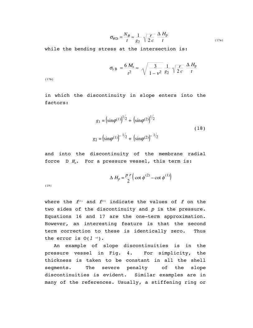
Fig. 4 – Pressure vessel with meridional slope

discontinuity at points C and D. The stress

distribution for a moderately thin shell

(Rs3/t = 100) is on the right. The O(l)

stress concentration at the points of slope

discontinuity is clear, in comparison with

the O(1) discontinuity at the points B and E

of curvature discontinuity. Dimensions are:

Rs1 = 20, Lc1 = 20, Rs2 = 200, Rs3 = 100, Lc2 =

84, f2 = p /6, f1 = 0.1, E = 0.3 x 108, n =

0.3, t = 1, p = 10.

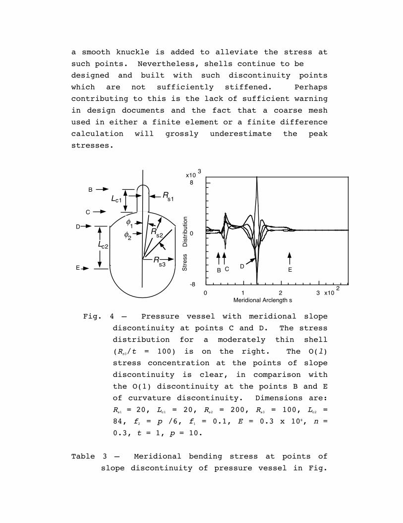
Table 3 – Meridional bending stress at points of

slope discontinuity of pressure vessel in Fig.

4. The asymptotic result is reasonable even

for the shallow region at point C.

Thi

ckn

ess

t

Pre

ssu

re

p

Poi

nt

2 –

ter

m

FAS

T1

1 10 C 0.2

49

x

104

0.2

83

x

104

D 0.8

37

x

104

0.8

40

x

104

0.1 1 C 0.7

89

x

104

0.7

83

x

104

D 0.2

65

x

105

0.2

64

x

105

3.5 Dimpling of Shell

The analysis of large displacement of thin shells

is generally a difficult problem. Guidance can be

found in Love's "principle of applicable surfaces"

(Ref. 17). Higher levels of strain energy are

required for deformations involving extensional

distortion of the reference surface, than are required

for inextensional bending. Consequently, even

elaborate post-buckling patterns are usually

characterized by regions of inextensional deformation

joined by lines of localized bending. Ashwell

(Ref. 1) uses this concept for the problem of a

spherical shell with a static radial point load, for

which the geometry is quite simple. He showed that a

good approximation can be obtained for the large

displacement behavior. The procedure consists of

assuming that a portion of the sphere, a "cap",

undergoes a curvature reversal and becomes a "dimple".

Continuity of stress and displacement is obtained by

solutions of the linear equations for the inverted cap

and the remaining portion of shell. Ashwell uses the

Bessel function solutions of the shallow shell

equations (Ref. 26). Ranjan and Steele (Ref. 24) show

that a much simpler solution can be obtained by using

the approximate edge stiffness coefficients (Eq. 6).

Furthermore, the accuracy is increased by including

the geometric nonlinearity from a perturbation

expansion of the moderate rotation equations by Ranjan

and Steele (Ref. 25).

3.5.1 Displacement Under Point Load. A spherical

shell under a point load P has the displacement x

according to the linear solution by Reissner (Ref. 26)

given by:

xt = P R 8 E t2c

= P* (20)

A simple solution is sought which will capture the

significant features of the nonlinear behavior.

Additional efforts are by Ranjan and Steele (Ref. 24)

and Libai and Simmonds (Ref. 16) to improve the

solution. A convenient form is obtained with the

assumption that the edge angle a of the inverted cap,

or dimple, shown in Fig. 1, is both "shallow":

α ≤ 0.3 (21)

and "steep":

Rc α >> 1

(22)

When the shell is thin enough, there is a range of

angles a which satisfy both Eqs. 21 and 22.

Adding the inverted dimple modifies the potential

energy. The dominant terms are external force

potential and the strain energy of bending of the

edges of the dimple and the remaining shell to obtain

continuity of the meridional slope. Note that the

angle of rotation c of each shell edge is equal to the

original angle a, which violates the assumptions of

the

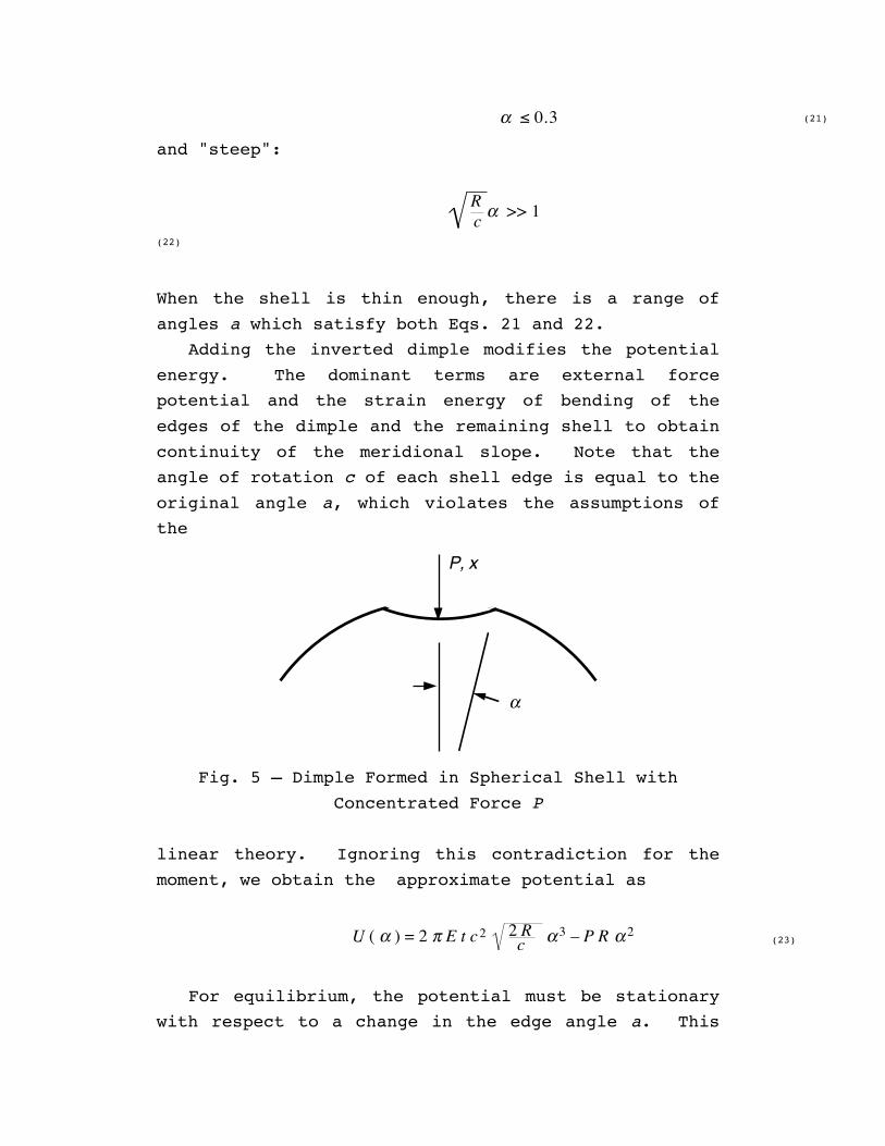
P, x

α

Fig. 5 – Dimple Formed in Spherical Shell with

Concentrated Force P

linear theory. Ignoring this contradiction for the

moment, we obtain the approximate potential as

U ( α ) = 2 π E t c2 2 Rc α3 – P R α 2 (23)

For equilibrium, the potential must be stationary

with respect to a change in the edge angle a. This

provides the relation between the edge angle and the

load magnitude P. Adding the linear result to the

additional displacement because of the dimpling gives

the total displacement:

xt = P* + K P* 2

(24)

where the constant is:

K = 8

3 π

23 1 – ν

2= 1.19 for ν = 0.3

(25)

To at least partially relieve the contradiction of

the large rotation, the nonlinear correction (Eq. 11)

can be used. Integrating to obtain the energy, and

setting the rotation equal to the angle a provides a

4/5 reduction in the strain energy and an increase in

the constant:

K NL = K

54

2= 1.86 for ν = 0.3

(26)

Using Eq. 26 in Eq. 24 gives a result which agrees

well with the experiments of Penning and Thurston

(Ref. 23) and the numerical results of Fitch (Ref. 9),

all on very thin spherical shells for displacement

magnitude up to about fifteen shell thicknesses. More

remarkable are the results of Taber (Ref. 37), showing

that the equivalent of Eq. 23 provides good agreement

with experiments on a thick shell ( R /t = 7). In

addition, Taber considered the problem of a shell

filled with an incompressible fluid, for which the

strain energy of the wall extension because of the

internal pressure must be added. The agreement

between calculation and experiment is reasonable for

displacements in magnitude up to about half the

radius.

Simo, et. al (Ref. 32), with resultant based

finite elements, find excellent agreement with Taber's

results when transverse shear deformation is

neglected. In computation with shear deformation

included (Simo, pers. comm.) the agreement is not as

good. It is possible that Taber chose a value of the

elastic modulus for the shell (a racket ball) to

obtain the good agreement. The adjustment for shear

deformation given by Eq. 7 is:

KNL+shear def = K 5

42

1 + β 2

1 + β /2

(27)

= 2.18 for n = 0.3, R /t =

7

Thus, the shear deformation for such a thick shell

should increase the displacement by 17 percent.

However, for the thick shells the conditions in Eqs.

21 and 22 cannot be satisfied. So any precise

agreement with reality should not be expected from Eq.

24. Another objection to this treatment is that in

the experiments and numerical computation by Fitch

(Ref. 9), bifurcations to nonsymmetric patterns occur.

However, a substantial load loss with such

bifurcations apparently does not take place, so the

symmetric solution remains a good approximation. This

analysis is restricted to dimples more than a decay

distance from any boundary, for which the displacement

increases with the load. When the decay distance

encounters a ring-stiffened edge, snap-through

buckling can occur, as discussed by Penning and

Thurston (Ref. 23).

3.5.2 Displacement Under Pressure. With external

pressure loading p, the volume displacement is needed

for the total potential change:

U ( α ) = 45 2 π E t c2 2 R

c α3 – p π4 R 3 α4 (28)

in which the nonlinear reduction factor of 4 /5 is

included. Because the potential now has a higher

power of the angle in the load term, the derivative of

this with respect to the angle gives an angle which is

inversely proportional to the pressure. This dimple

gives, therefore, an unstable equilibrium curve. The

volume displacement DV is:

Δ V8 p R 2 c

= 1 – ν ρ + cR

3 25 ρ

4 (29)

in which the prestress factor (Eq. 8) is

ρ = – p R 2

4 E t c (30)

The classical bifurcation occurs at r = – 1; Eq. 29

gives the post-buckling curve for values of r small

in comparison with unity.

3.5.3 Displacement Under Line Load. With a line

load of intensity q the cross-sectional area

displacement is needed for the total potential:

U ( α ) = 45 2 π E t c2 2 R

c α3 – q 43 R 2 α3 (31)

For the line load, the same power of the angle a

occurs in the strain energy and load terms. Thus, the

nontrivial solution is a state of neutral equilibrium.

Setting Eq. 31 to zero gives the magnitude of the

critical line load to be:

qcr = 45 3 π

2 E t cR

2 cR

(32)

It is of interest to calculate the linear solution

for the concentrated line load at the equator of the

sphere. The bifurcation estimate obtained by setting

Eq. 8 equal to unity is only 6 percent higher than Eq.

32. The conclusion is that the line load will not be

imperfection sensitive, because neutral equilibrium is

maintained as the dimples form when the load is near

the classical bifurcation value. The significant

condition on the edge effect solution is a radial line

load in such problems as the shell without radial

constraint in Fig. 3 and the regions of slope

discontinuity in Fig. 4. The conclusion is that the

local instability in such problems also will not be

imperfection sensitive, so that the classical

bifurcation load will be a good indication of the

actual load capability.

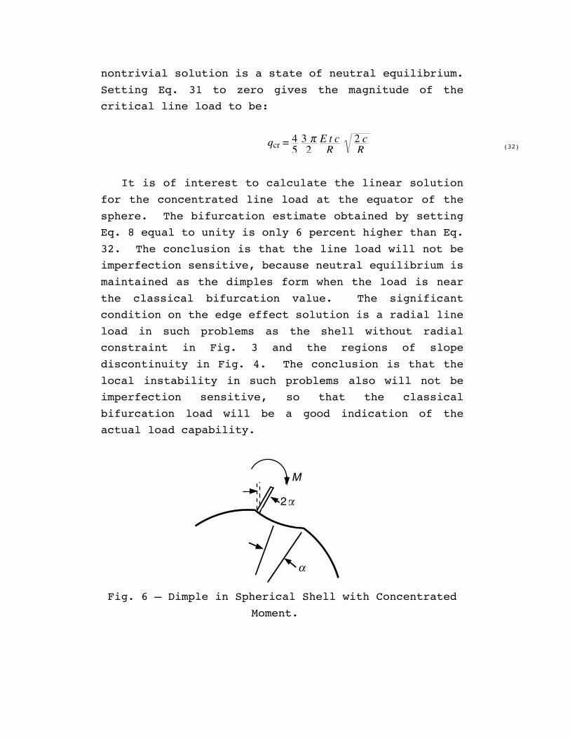
α

α2

M

Fig. 6 – Dimple in Spherical Shell with Concentrated

Moment.

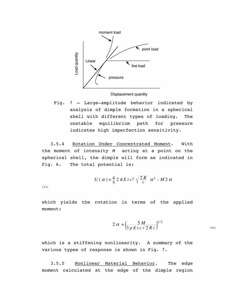
Displacement quantity

Load

qua

ntity

Linear

pressure

line load

point load

moment load

Fig. 7 – Large-amplitude behavior indicated by

analysis of dimple formation in a spherical

shell with different types of loading. The

unstable equilibrium path for pressure

indicates high imperfection sensitivity.

3.5.4 Rotation Under Concentrated Moment. With

the moment of intensity M acting at a point on the

spherical shell, the dimple will form as indicated in

Fig. 6. The total potential is:

U ( α ) = 45 2 π E t c2 2 R

c α3 – M 2 α

(33)

which yields the rotation in terms of the applied

moment:

2 α = 5 M

3 p E t c 2 R c1/2

(34)

which is a stiffening nonlinearity. A summary of the

various types of response is shown in Fig. 7.

3.5.5 Nonlinear Material Behavior. The edge

moment calculated at the edge of the dimple region

from Eq. 5 indicates that the yield stress of a

metallic shell with moderate R /t values will be

exceeded before the dimple becomes very large. For a

rough indication of the behavior, an elastic-plastic,

moment-curvature relation can be considered. As the

dimple increases, each point on the sphere wall will

experience, first, a substantial curvature increase

and then, a reversed bending to reach the final

curvature of opposite sign in the inner dimple region.

If a reversible, nonlinear elastic material is

considered, the analysis follows the same line of

reasoning as used in the preceding sections. The

significant strain energy is just that to bend the

edge of the dimple and the edge of the outer portion

of the shell, each through the angle of a. The total

potential for the point load is just:

U ( α ) = Mu 2 π R α ( 2 α ) – P R α 2 (35)

in which Mu is the yield moment of the shell wall.

Now both terms have the same power of a, so the

equilibrium is neutral, with the critical collapse

value of the load:

Pcr = 4 π Mu (36)

If the total work W of the external force is

prescribed, the maximum displacement is:

x = W

4 π Mu (37)

Following the similar analysis for the other load

cases indicates that both the line load and pressure

load will have unstable post-buckling equilibrium

paths. Experiments and computations on the residual

permanent deformation because of impact of spherical

shells are reported by Witmer, et. al (Ref. 40). The

estimate in Eq. 37 exceeds their values by a factor of

3, which is not surprising because Eq. 35 does not

consider the actual plastic work. However, it is

curious that Eqs. 36 and 37 are independent of the

shell geometry. More extensive study of this problem

using the dimple may be warranted.

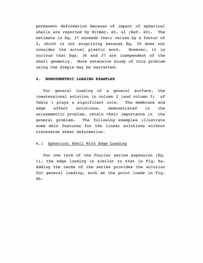
4. NONSYMMETRIC LOADING EXAMPLES

For general loading of a general surface, the

inextensional solution in column 2 (and column 5) of

Table 1 plays a significant role. The membrane and

edge effect solutions, demonstrated in the

axisymmetric problem, retain their importance in the

general problem. The following examples illustrate

some main features for the linear solutions without

transverse shear deformation.

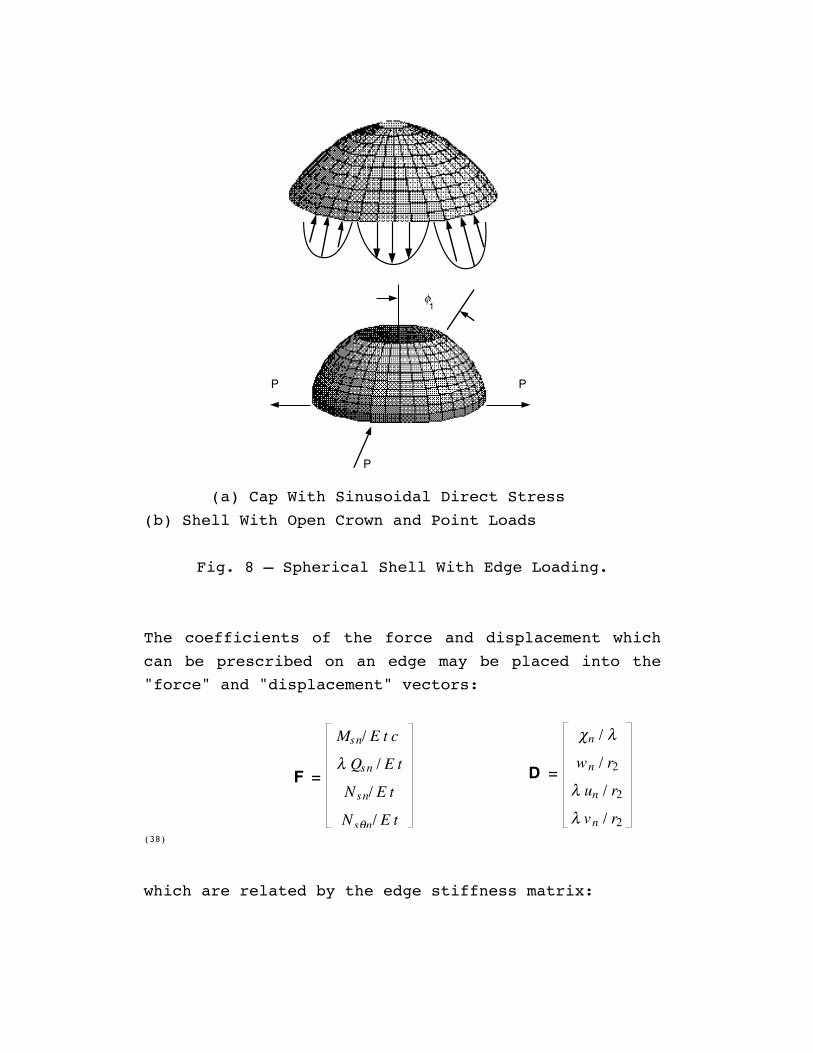
4.1 Spherical Shell With Edge Loading

For one term of the Fourier series expansion (Eq.

1), the edge loading is similar to that in Fig. 8a.

Adding the terms of the series provides the solution

for general loading, such as the point loads in Fig.

8b.

P

P

P

φ1

(a) Cap With Sinusoidal Direct Stress

(b) Shell With Open Crown and Point Loads

Fig. 8 – Spherical Shell With Edge Loading.

The coefficients of the force and displacement which

can be prescribed on an edge may be placed into the

"force" and "displacement" vectors:

F =

Msn/ E t c

λ Qsn / E t

Nsn/ E t

Nsθn/ E t

D =

χn / λ

wn / r2λ un / r2λ vn / r2

(38)

which are related by the edge stiffness matrix:

F = K• D (39)

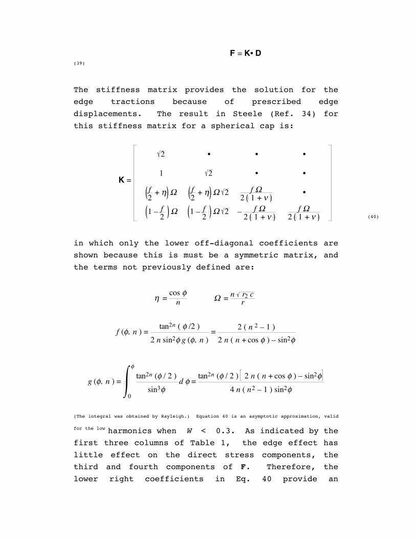
The stiffness matrix provides the solution for the

edge tractions because of prescribed edge

displacements. The result in Steele (Ref. 34) for

this stiffness matrix for a spherical cap is:

K =

2 • • •

1 2 • •

f2 + η Ω f

2 + η Ω 2 f Ω2 1 + ν

•

1 – f2 Ω 1 – f2 Ω 2 – f Ω2 1 + ν

f Ω2 1 + ν (40)

in which only the lower off-diagonal coefficients are

shown because this is must be a symmetric matrix, and

the terms not previously defined are:

η = cos φ

n Ω = n r2 cr

f (φ, n ) = tan2n ( φ /2 )

2 n sin2φ g (φ, n ) = 2 ( n 2 – 1 )

2 n ( n + cos φ ) – sin2φ

g (φ, n ) = tan2n (φ / 2 )

sin3φ d φ

0

φ

= tan2n (φ / 2 ) 2 n ( n + cos φ ) – sin2φ

4 n ( n2 – 1 ) sin2φ

(The integral was obtained by Rayleigh.) Equation 40 is an asymptotic approximation, valid

for the low harmonics when W < 0.3. As indicated by the

first three columns of Table 1, the edge effect has

little effect on the direct stress components, the

third and fourth components of F. Therefore, the

lower right coefficients in Eq. 40 provide an

excellent check on the proper computation of the

membrane behavior. The upper left coefficients in

Eq. 40 are primarily because of the edge effect, while

the off-diagonal blocks of coefficients depend on all

three types of solutions.

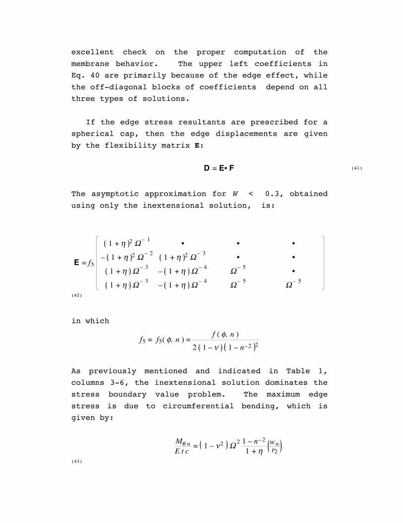
If the edge stress resultants are prescribed for a

spherical cap, then the edge displacements are given

by the flexibility matrix E:

D = E• F (41)

The asymptotic approximation for W < 0.3, obtained

using only the inextensional solution, is:

E = f5

1 + η 2 Ω – 1 • • •

– 1 + η 2 Ω – 2 1 + η 2 Ω – 3 • •

1 + η Ω – 3 – 1 + η Ω – 4 Ω – 5 •

1 + η Ω – 3 – 1 + η Ω – 4 Ω – 5 Ω – 5

(42)

in which

f5 = f5( φ, n ) = f ( φ, n )

2 1 – ν 1 – n–2 2

As previously mentioned and indicated in Table 1,

columns 3-6, the inextensional solution dominates the

stress boundary value problem. The maximum edge

stress is due to circumferential bending, which is

given by:

Mθ nE t c

= 1 – ν2 Ω 2 1 – n–21 + η

wnr2

(43)

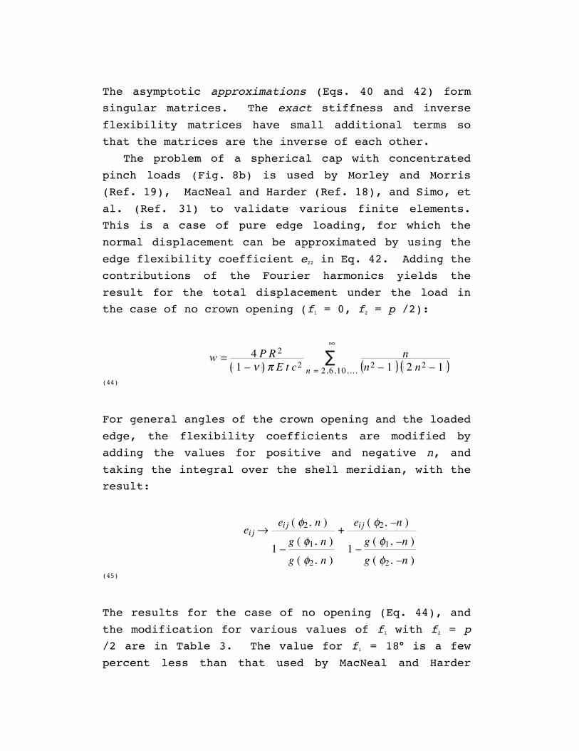
The asymptotic approximations (Eqs. 40 and 42) form

singular matrices. The exact stiffness and inverse

flexibility matrices have small additional terms so

that the matrices are the inverse of each other.

The problem of a spherical cap with concentrated

pinch loads (Fig. 8b) is used by Morley and Morris

(Ref. 19), MacNeal and Harder (Ref. 18), and Simo, et

al. (Ref. 31) to validate various finite elements.

This is a case of pure edge loading, for which the

normal displacement can be approximated by using the

edge flexibility coefficient e22 in Eq. 42. Adding the

contributions of the Fourier harmonics yields the

result for the total displacement under the load in

the case of no crown opening (f1 = 0, f2 = p /2):

w = 4 P R 2

1 – ν π E t c2 n

n2 – 1 2 n2 – 1 ∑

n = 2,6,10,.. .

∞

(44)

For general angles of the crown opening and the loaded

edge, the flexibility coefficients are modified by

adding the values for positive and negative n, and

taking the integral over the shell meridian, with the

result:

ei j → ei j ( φ2, n )

1 – g ( φ1, n )g ( φ2, n )

+ ei j ( φ2, –n )

1 – g ( φ1, –n )g ( φ2, –n )

(45)

The results for the case of no opening (Eq. 44), and

the modification for various values of f1 with f2 = p

/2 are in Table 3. The value for f1 = 18° is a few

percent less than that used by MacNeal and Harder

(Ref. 18), and Simo, et al. (Ref. 31). The opening

has little effect until the angle becomes rather

large, which is because of the elliptic nature of the

inextensional equations for the shell of positive

curvature. Also clear from the rapid convergence of

the series (Eq. 44) is that the main

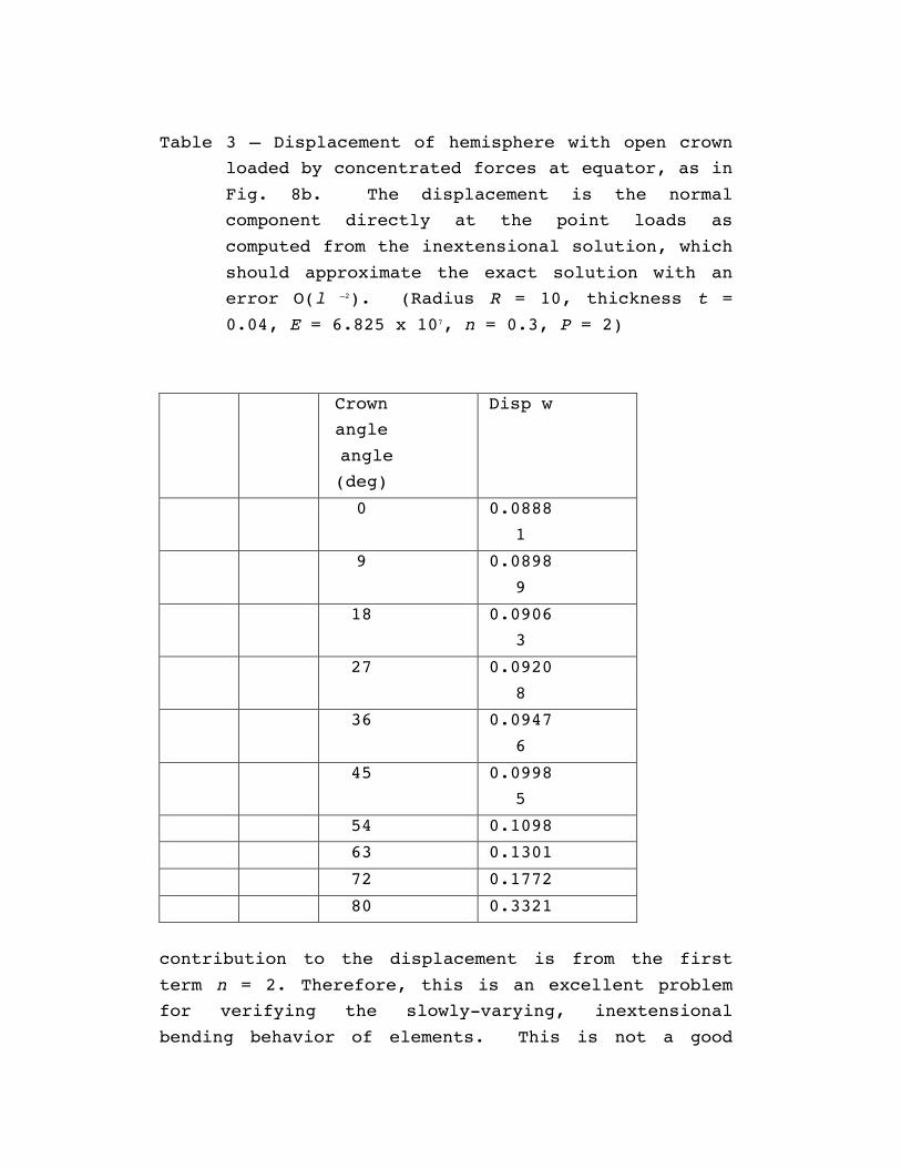
Table 3 – Displacement of hemisphere with open crown

loaded by concentrated forces at equator, as in

Fig. 8b. The displacement is the normal

component directly at the point loads as

computed from the inextensional solution, which

should approximate the exact solution with an

error O(l –2). (Radius R = 10, thickness t =

0.04, E = 6.825 x 107, n = 0.3, P = 2)

Crown

angle

angle

(deg)

Disp w

0 0.0888

1

9 0.0898

9

18 0.0906

3

27 0.0920

8

36 0.0947

6

45 0.0998

5

54 0.1098

63 0.1301

72 0.1772

80 0.3321

contribution to the displacement is from the first

term n = 2. Therefore, this is an excellent problem

for verifying the slowly-varying, inextensional

bending behavior of elements. This is not a good

example for stress, because the series is divergent,

giving the logarithmic singularity at the point load.

A suggestion is to use a distribution of load, such as

in Fig. 8a, particularly the harmonic n = 2. For

this, the result (Eq. 42) should be a good

comparison.

For a thorough verification, all the coefficients

in the matrices (Eqs. 40 and 42) should be confirmed

for the harmonic n = 2. A coarse mesh should be

adequate for the flexibility matrix, which verifies

the inextensional performance, and for the lower,

right-hand block in the stiffness matrix, which

verifies the membrane performance. The upper, left-

hand block and the off-diagonal blocks in the

stiffness matrix depend on the edge effect. For

these, a fine mesh is necessary, similar to that

discussed for the axisymmetric shell.

Because the columns in the flexibility matrix (Eq.

42) are proportional, certain combinations of edge

load components will produce zero displacement,

according to this asymptotic approximation. In fact,

such a combination of loads is a special case which

will satisfy the boundary conditions of the membrane

and edge effects exactly. To demonstrate this,

consider the following result for the meridional

displacement of the hemisphere because of prescribed

values of the direct stress resultants at the edge:

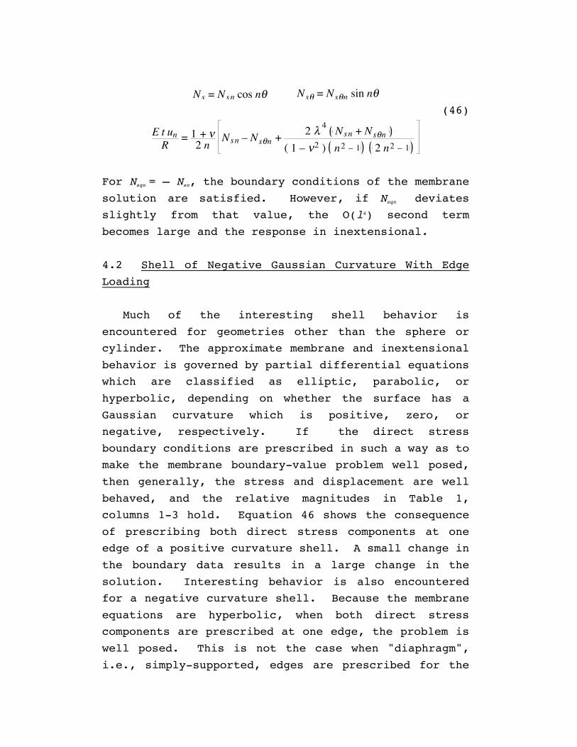
Ns = Nsn cos nθ Nsθ = Nsθn sin nθ (46)

E t unR

= 1 + ν2 n

Nsn – Nsθn + 2 λ 4 Nsn + Nsθn ( 1 – ν2 ) n2 – 1 2 n2 – 1

For Nsqn = – Nsn, the boundary conditions of the membrane

solution are satisfied. However, if Nsqn deviates

slightly from that value, the O(l4) second term

becomes large and the response in inextensional.

4.2 Shell of Negative Gaussian Curvature With Edge

Loading

Much of the interesting shell behavior is

encountered for geometries other than the sphere or

cylinder. The approximate membrane and inextensional

behavior is governed by partial differential equations

which are classified as elliptic, parabolic, or

hyperbolic, depending on whether the surface has a

Gaussian curvature which is positive, zero, or

negative, respectively. If the direct stress

boundary conditions are prescribed in such a way as to

make the membrane boundary-value problem well posed,

then generally, the stress and displacement are well

behaved, and the relative magnitudes in Table 1,

columns 1-3 hold. Equation 46 shows the consequence

of prescribing both direct stress components at one

edge of a positive curvature shell. A small change in

the boundary data results in a large change in the

solution. Interesting behavior is also encountered

for a negative curvature shell. Because the membrane

equations are hyperbolic, when both direct stress

components are prescribed at one edge, the problem is

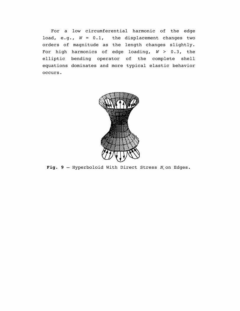
well posed. This is not the case when "diaphragm",

i.e., simply-supported, edges are prescribed for the

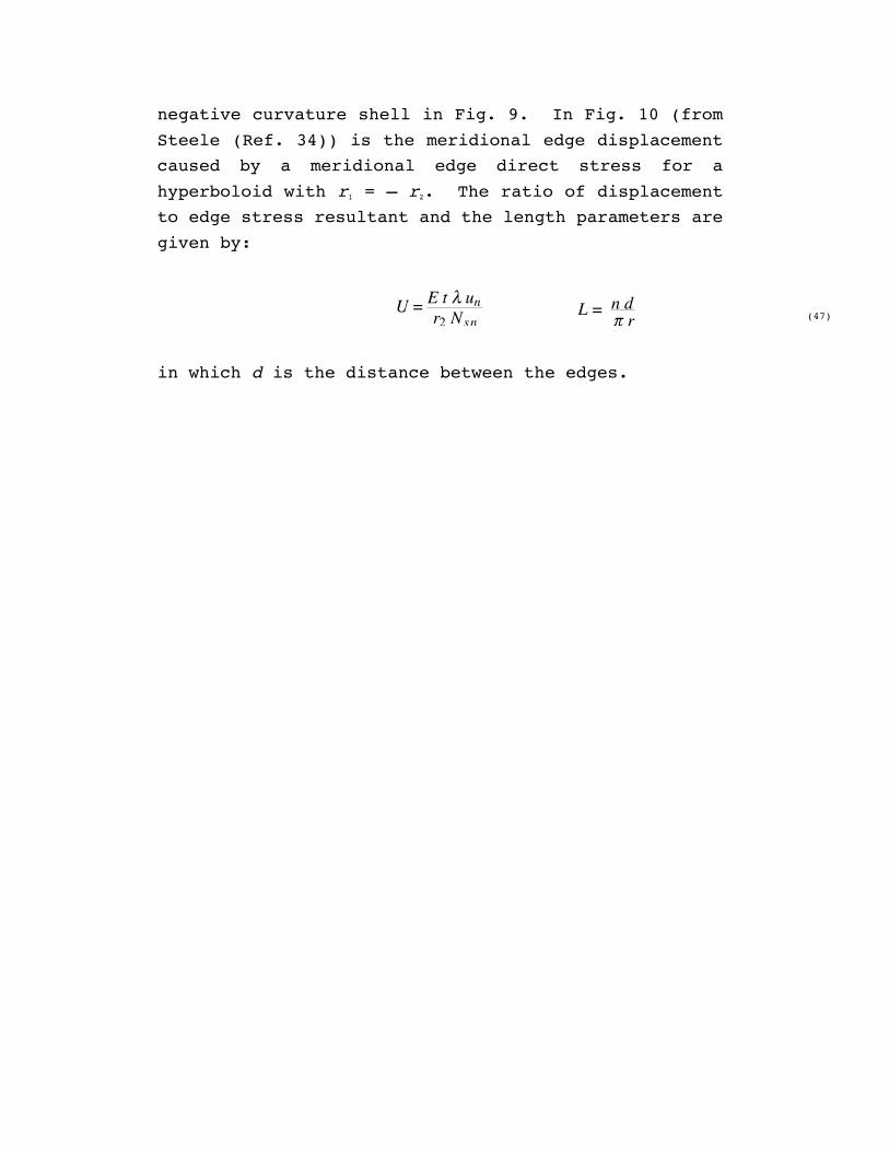
negative curvature shell in Fig. 9. In Fig. 10 (from

Steele (Ref. 34)) is the meridional edge displacement

caused by a meridional edge direct stress for a

hyperboloid with r1 = – r2. The ratio of displacement

to edge stress resultant and the length parameters are

given by:

U = E t λ un

r2 Nsn

L = n dπ r

(47)

in which d is the distance between the edges.

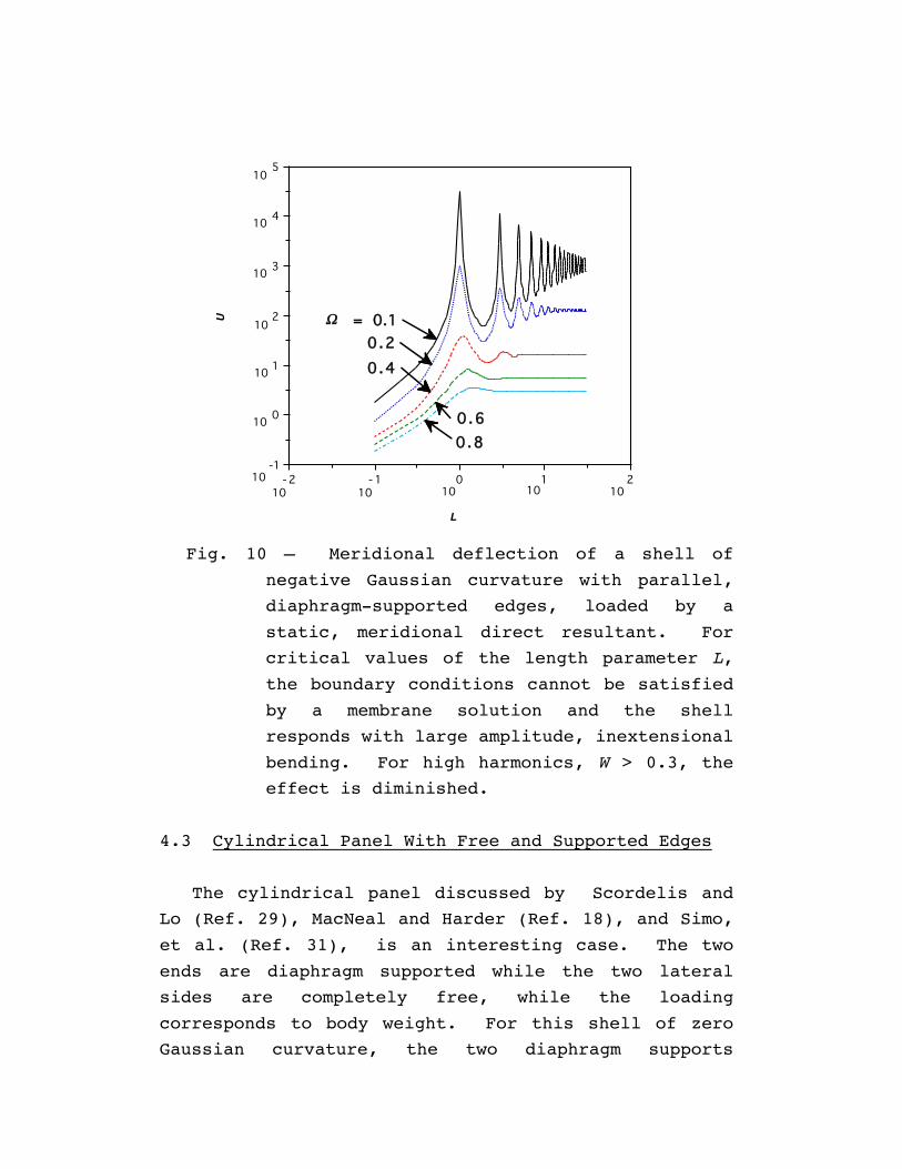
For a low circumferential harmonic of the edge

load, e.g., W = 0.1, the displacement changes two

orders of magnitude as the length changes slightly.

For high harmonics of edge loading, W > 0.3, the

elliptic bending operator of the complete shell

equations dominates and more typical elastic behavior

occurs.

Fig. 9 – Hyperboloid With Direct Stress Ns on Edges.

210- 1- 2-1

0

1

2

3

4

5

L

U

10

10

10

10

10

10

10

10 10 10 10 10

Ω = 0.10 .20 .4

0 .60 .8

Fig. 10 – Meridional deflection of a shell of

negative Gaussian curvature with parallel,

diaphragm-supported edges, loaded by a

static, meridional direct resultant. For

critical values of the length parameter L,

the boundary conditions cannot be satisfied

by a membrane solution and the shell

responds with large amplitude, inextensional

bending. For high harmonics, W > 0.3, the

effect is diminished.

4.3 Cylindrical Panel With Free and Supported Edges

The cylindrical panel discussed by Scordelis and

Lo (Ref. 29), MacNeal and Harder (Ref. 18), and Simo,

et al. (Ref. 31), is an interesting case. The two

ends are diaphragm supported while the two lateral

sides are completely free, while the loading

corresponds to body weight. For this shell of zero

Gaussian curvature, the two diaphragm supports

eliminate the possibility of a dominant inextensional

deformation, which would give the relations in Table

1, columns 4-6. However, it is impossible to obtain a

membrane solution, which would give the relations in

Table 1, columns 1-3, because of the free lateral edge

condition. This is a case of the boundary which is

tangent to an asymptotic line on the surface,

discussed by Gol'denweiser (Ref. 12). On the lateral

edges r2 -> infinity, and the decay distance of the

edge effect from Eq. 4 is infinite. This is a

degenerate situation in which all solutions are slowly

varying over the shell, requiring only a course mesh

of elements. To see the behavior, the asymptotic

approximation for the flexibility coefficient e23 is

extracted from Steele (Ref. 34), which yields the

approximation for the normal displacement at the

center of the free edge:

disp = 5.82 L2

π 2 R c p R 2

E t (48)

This approximation is valid for the very thin, shallow

panel. From Scordelis and Lo (Ref. 29) the values p =

90, R = 25, L = 50, t = 0.25, E = 4.32x108, v = 0,

with the edge angle of 40°, give the displacement

0.309, while Eq. 48 gives the displacement 0.43.

Because the panel is not shallow and not exceptionally

thin, the approximation is reasonable. More important

is that Eq. 48 shows that the displacement is O(l2) in

comparison with the membrane solution, halfway between

the two stress states in Table 1.

The conclusion is that the two shell problems used

by MacNeal and Harder, (Ref. 18), consisting of the

cylindrical panel and the open hemisphere with the

point loads (Fig. 8b), are excellent problems but do

not cover the full range of shell behavior. In both,

the dominant state of deformation is slowly varying

and can be handled by a coarse mesh. A serious

objection is that no consideration of the stress is

made. In the panel problem, the stress is also slowly

varying, so accurate results should be obtainable with

the coarse mesh. In the point load problem, however,

the interesting stress occurs exactly at the point

load and has a logarithmic singularity, as in the flat

plate bending problem. As previously mentioned, a

thorough verification requires consideration of a

single, low harmonic of boundary conditions to ensure

the accuracy of both membrane and inextensional

displacements and stress.

R RM

M

αβ

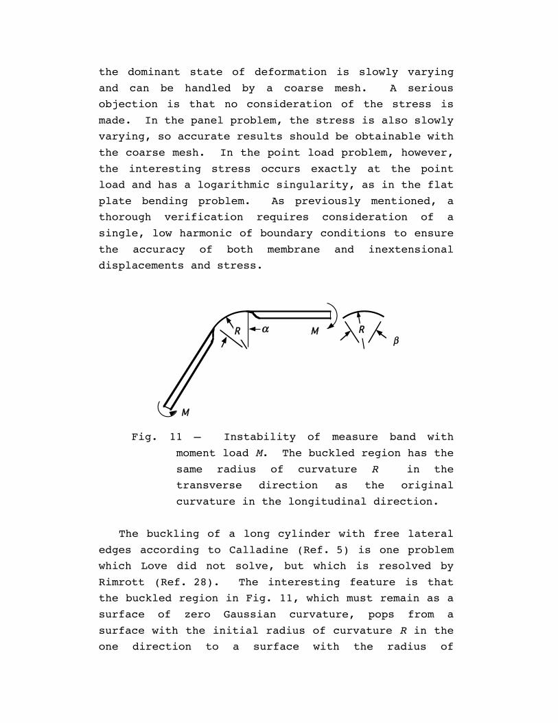
Fig. 11 – Instability of measure band with

moment load M. The buckled region has the

same radius of curvature R in the

transverse direction as the original

curvature in the longitudinal direction.

The buckling of a long cylinder with free lateral

edges according to Calladine (Ref. 5) is one problem

which Love did not solve, but which is resolved by

Rimrott (Ref. 28). The interesting feature is that

the buckled region in Fig. 11, which must remain as a

surface of zero Gaussian curvature, pops from a

surface with the initial radius of curvature R in the

one direction to a surface with the radius of

curvature R in the orthogonal direction. This seems

to be the equivalent of the dimple for a surface of

positive curvature. The potential for this is:

U = E t c2 ( 1 – ν ) β α – M α (49)

Because the strain energy of the buckled region and

the potential of the external moment are both

proportional to the angle a, the solution gives

neutral equilibrium with the critical moment:

Mcr = E t c2 ( 1 – ν ) β (50)

The classical buckling load, obtained from the

membrane solution and the local instability condition

Eq. 10, is:

Mcl = 815 E t c R β 3

(51)

which is O(l2) higher. Thus, Eq. 50 gives a low,

post-buckling plateau in the moment-angle

relationship. Returning to the problem of the panel

loaded by weight and with diaphragm supports at the

ends, one may consider the post-buckling behavior with

a "yield hinge" of magnitude (Eq. 50) at the center,

which yields the critical weight magnitude of:

pcr = 2 E t c2 ( 1 – ν )

R L2 (52)

For the dimensions of Scordelis and Lo (Ref. 29), this

gives pcr = 18. It will be interesting to see the

post-buckling behavior for this problem from a direct,

nonlinear, finite element calculation for displacement

large in comparison with the shell thickness.

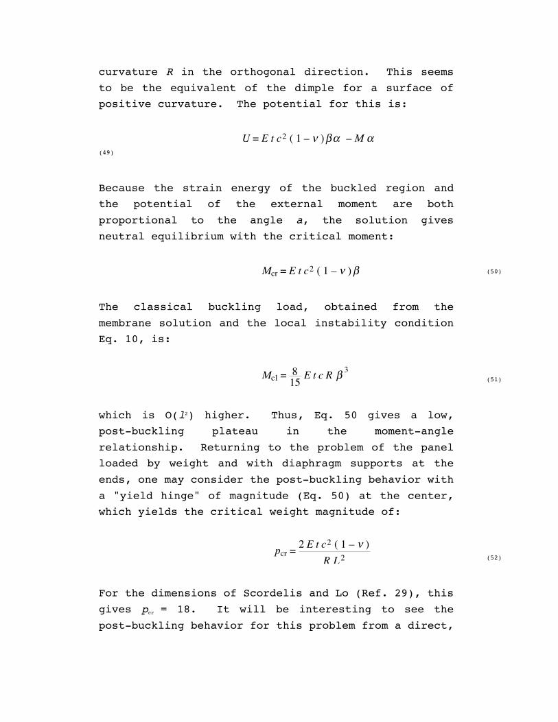
4.4 Nearly Concentrated Line Load

Concentrated effects in shells are important. To

avoid the singularity of the point load, however, a

localized line load such as those shown in Fig. 12 can

be used. The distribution of the line load intensity

in the circumferential direction is:

q θ = qmax1 + 3 θ / θq

2 (53)

in which qq is the angle at which the intensity is 10

percent of the maximum value. The arc length between

the 10 percent points is d = 2r qq . The total force

is:

P = qmaxπ d /6 (54)

In unpublished work based on Steele (Ref. 34), Fourier

integrals were used for the following results. For a

region of the surface of positive Gaussian curvature,

the maximum displacement under the load is given by:

wmax = P rm

8 E t c Fdisp Ω, ν

(55)

d

Fig. 12 – Shell with line load of bell-shaped

distribution in region of positive curvature

and in region of negative curvature. The

width of the distribution is d, measured to

the points at which the intensity is 0.1 of

the maximum value.

in which the mean radius of curvature is:

1rm

= 12 1r1 + 1r2 (56)

and the factor Fdisp depends on Poisson's ratio and the

parameter:

Ω = 6 c r2

d (57)

The limiting behavior is:

Fdisp → r2

r1 + 1 2

π Ω for Ω → 0

→ 1

for Ω → ∞, r2r1

= 1 (58)

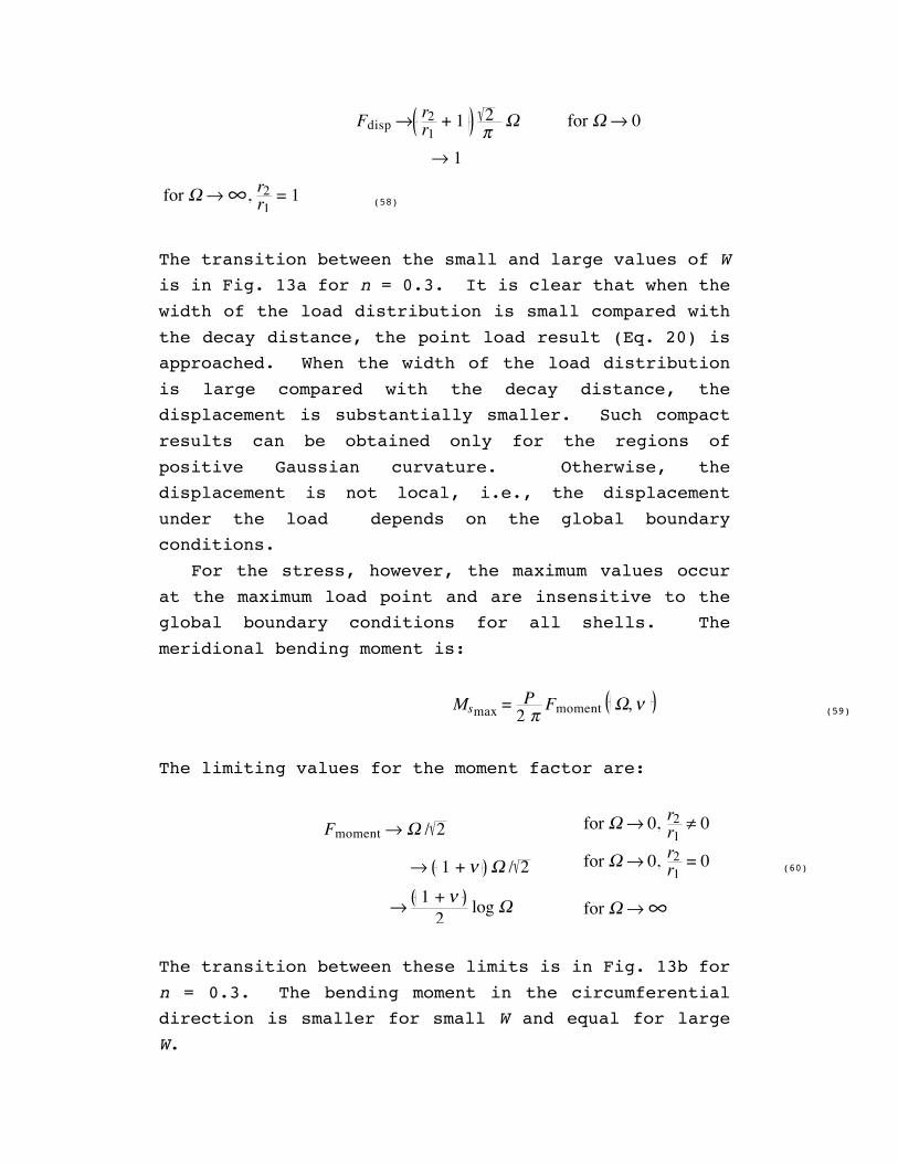
The transition between the small and large values of W

is in Fig. 13a for n = 0.3. It is clear that when the

width of the load distribution is small compared with

the decay distance, the point load result (Eq. 20) is

approached. When the width of the load distribution

is large compared with the decay distance, the

displacement is substantially smaller. Such compact

results can be obtained only for the regions of

positive Gaussian curvature. Otherwise, the

displacement is not local, i.e., the displacement

under the load depends on the global boundary

conditions.

For the stress, however, the maximum values occur

at the maximum load point and are insensitive to the

global boundary conditions for all shells. The

meridional bending moment is:

Msmax = P

2 π Fmoment Ω, ν

(59)

The limiting values for the moment factor are:

Fmoment → Ω / 2 for Ω → 0, r2

r1 ≠ 0

→ 1 + ν Ω / 2 for Ω → 0, r2r1

= 0 (60)

→ 1 + ν

2 log Ω

for Ω → ∞

The transition between these limits is in Fig. 13b for

n = 0.3. The bending moment in the circumferential

direction is smaller for small W and equal for large

W.

The circumferential direct stress is:

Nθmax = P

2 π t c Fdirect Ω, ν

(61)

The limiting values for the direct stress factor are:

Fdirect → Ω / 2 for Ω → 0

→ constant for Ω → ∞

(62)

The transition between these limits is in Fig. 13c

for n = 0.3. The direct stress in the meridional

direction is smaller for small W and equal for large

W. The transition in Figs. 13a-c from the elementary

shell solutions estimated in Table 1 to the local

point load is an important part of shell behavior,

which should be properly represented in a numerical

computation.

5. COMPUTER IMPLEMENTATION

The approximate solutions in the preceding

sections are "closed form" or obtained with a

relatively little amount of computation, as for Fig.

13. Generally, such solutions can be obtained from a

formal asymptotic expansion procedure. As a rule, the

asymptotic expansion is designed to take advantage of

the feature of the problem which makes direct

numerical computation difficult. A natural question

is whether or not the asymptotic approach can be used

in a numerical procedure. The difficulty for shells

is that such a battery of different asymptotic

techniques are used for the variety of problems.

Limits of applicability and/or error estimates are

often difficult to obtain or are too conservative. It

is no wonder that the overwhelming emphasis in the

last years has been on developing finite element

techniques sufficiently robust so that a user can

solve real shell problems without the prerequisite of

having to spend years learning the information in the

references. However, shells present difficulties to

such an approach as well. Shell problems are of such

a nature

that all the information and techniques which are at

our disposal should be used, including finite element

and asymptotic methods.

432100.0

0.2

0.4

0.6

0.8

1.0

1.2

Ω

Fdis

p 1 = r /r2 1

5

3

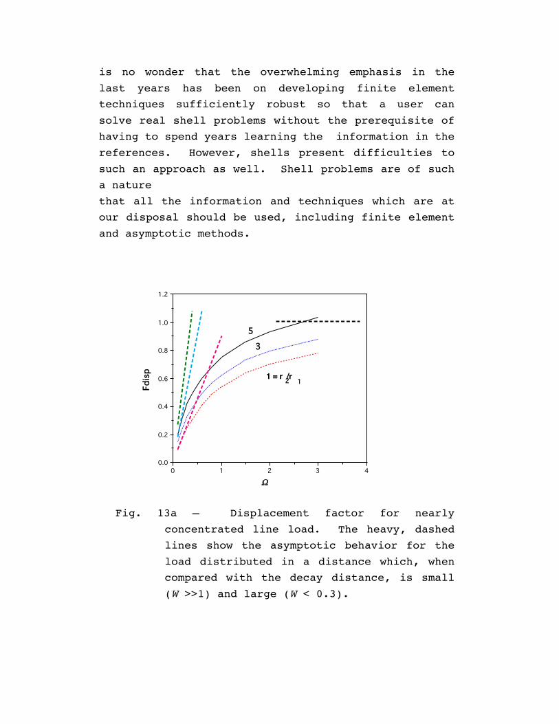
Fig. 13a – Displacement factor for nearly

concentrated line load. The heavy, dashed

lines show the asymptotic behavior for the

load distributed in a distance which, when

compared with the decay distance, is small

(W >>1) and large (W < 0.3).

5432100.0

0.5

1.0

1.5

Ω

Fmom

ent

r /r = 02 1

–1

–5

1

5

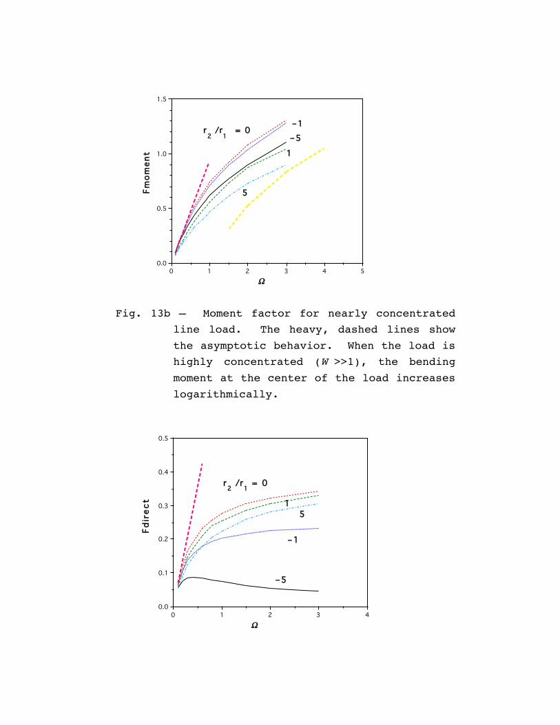
Fig. 13b – Moment factor for nearly concentrated

line load. The heavy, dashed lines show

the asymptotic behavior. When the load is

highly concentrated (W >>1), the bending

moment at the center of the load increases

logarithmically.

432100.0

0.1

0.2

0.3

0.4

0.5

Ω

Fdir

ect

r /r = 02 1

15

–1

–5

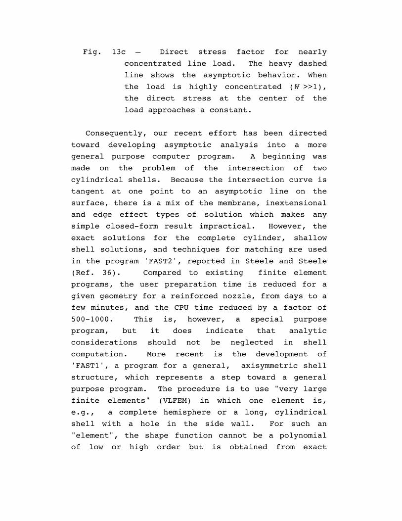
Fig. 13c – Direct stress factor for nearly

concentrated line load. The heavy dashed

line shows the asymptotic behavior. When

the load is highly concentrated (W >>1),

the direct stress at the center of the

load approaches a constant.

Consequently, our recent effort has been directed

toward developing asymptotic analysis into a more

general purpose computer program. A beginning was

made on the problem of the intersection of two

cylindrical shells. Because the intersection curve is

tangent at one point to an asymptotic line on the

surface, there is a mix of the membrane, inextensional

and edge effect types of solution which makes any

simple closed-form result impractical. However, the

exact solutions for the complete cylinder, shallow

shell solutions, and techniques for matching are used

in the program 'FAST2', reported in Steele and Steele

(Ref. 36). Compared to existing finite element

programs, the user preparation time is reduced for a

given geometry for a reinforced nozzle, from days to a

few minutes, and the CPU time reduced by a factor of

500-1000. This is, however, a special purpose

program, but it does indicate that analytic

considerations should not be neglected in shell

computation. More recent is the development of

'FAST1', a program for a general, axisymmetric shell

structure, which represents a step toward a general

purpose program. The procedure is to use "very large

finite elements" (VLFEM) in which one element is,

e.g., a complete hemisphere or a long, cylindrical

shell with a hole in the side wall. For such an

"element", the shape function cannot be a polynomial

of low or high order but is obtained from exact

solutions or asymptotic approximations properly

corrected.

6. CONCLUSION

The thin shell is an intriguing device with many

contradictions. Compared to flat plate and beam

structures, great material savings are possible. On

the other hand, the potential for great catastrophe is

always present. Extremely simple approximate theory

and solutions have provided the basis for shell design

for more than 100 years. On the other hand, a

satisfactory first approximation theory is relatively

recent. The general equations for static loading are

elliptic, so St. Venant's principle holds. On the

other hand, the reduced equations for the membrane and

inextensional behavior are hyperbolic for shells of

negative curvature, so St. Venant's principle may not

hold. A requirement for a well-posed problem of

mathematical physics is that the solution be

continuously dependent upon the parameters. On the

other hand, as indicated for the spherical shell with

stress boundary conditions (Eq. 46) and the shell of

negative curvature with diaphragm-supported edges in

Fig. 10, the change in the solution because of a small

change in the parameters can be quite large.

To capture such possibilities, it appears that a

validation of a numerical program for analysis of

shells should be subjected to a substantially more

demanding array of benchmark problems than has been

used in the past. The problems described in this

paper represent a minimal beginning.

That approximate results for special problems can

be obtained with minimal computation should not be

ignored in future development. Even with future

generations of computers, problems involving

optimization and dynamic response of complex shell

structures will remain of excessive cost with the

currently available shell elements and mesh generation

techniques. We may look forward to numerical

procedures in which the best features of current

finite elements and asymptotic analysis are exploited

fully. The thin shell is sufficiently demanding that

all the techniques at our disposal, analytical and

numerical, can be fruitfully employed.

ACKNOWLEDGEMENT

This work is supported by a grant from the

National Science Foundation. The stimulation for the

paper came from discussions with J. Simo. I also

thank Y. Y. Kim and B. D. Steele for helpful comments.

REFERENCES

1. Ashwell, D. G., "On the Large Deflection of a

Spherical Shell With An Inward Point Load", Theory of Thin Elastic Shells, W. Koiter (ed.), North-Holland, Amsterdam, 1960, pp. 44-63.

2. Axelrad, E., Schalentheorie, Teubner, Stuttgart, 1983.

3. Bushnell, D., Computerized Buckling Analysis of Shells, Martinus Nijhoff, Dordrecht, Netherlands, 1985.

4. Calladine, C. R., Theory of Shell Structures, Cambridge University Press, 1983.

5. Calladine, C. R., "The Theory of Thin Shell Structures, 1888-1988", Love Centenary Lecture, Proceedings of the Institute of Mechanical Engineers, Vol. 202, No. 42, 1988.

6. Donnell, L. H., Beams, Plates, and Shells, McGraw-Hill, New York, 1976.

7. Dowell, E. H., Aeroelasticity of Plates and Shells, Noordhoff, Holland, 1975.

8. Dym, C. L., Introduction to the Theory of Shells, Pergamon, 1974.

9. Fitch, J. R., "The Buckling and Post-Buckling Behavior of Spherical Caps Under Concentrated

Load", International Journal of Solids and Structures, Vol. 4, 1968, pp. 421-446.

10. Flügge, W., Stresses in Shells, Springer, Berlin, 1973.

11. Gibson, J. E., Thin Shells, Computing and Theory, Pergamon, 1980.

12. Gol'denweiser, A. L., Theory of Elastic Thin Shells, Pergamon, 1961.

13. Gould, P. L., Static Analysis of Shells, Lexington Books, Lexington, Mass., 1977.

14. Hoff, N. J., and Soong, T. C., "Buckling of Circular Cylindrical Shells in Axial Compression", International Journal of Mechanical Science, Vol. 7, 1965, pp. 489-520.

15. Kraus, H., Thin Elastic Shells, Wiley, New York, 1967.

16. Libai, A., and Simmonds, J. G., The Nonlinear Theory of Elastic Shells - One Spatial Dimension, Academic Press, 1988.

17. Love, A. E. H., A Treatise On the Mathematical Theory of Elasticity, 4th ed., Cambridge University Press, 1927, (reprinted by Dover, New York, 1944).

18. MacNeal, R. H., and Harder, R. L.,"A Proposed Standard Set of Problems to Test Finite Element Accuracy", Finite Elements in Analysis and Design, Vol 1, 1985, pp. 3-20.

19. Morley, L. S. D., and Morris, A. J., "Conflict between finite elements and shell theory", Royal Aircraft Establishment Report, London, 1978.

20. Naghdi, P. M., "The Theory of Shells and Plates", in Handbüch der Physik, VI a/2 Springer, Berlin, 1972.

21. Niordson, F. I., Introduction to Shell Theory, 1980.

22. Novozhilov, V. V., The Theory of Shells, Noordhoff, Holland, 1959.

23. Penning, F. A., and Thurston, G. A., "The Stability of Shallow Spherical Shells Under Concentrated Load", NASA CR-265, 1965.

24. Ranjan, G. V., and Steele, C. R., "Large Deflection of Deep Spherical Shells Under Concentrated Load", Proceedings of the 18th Structures, Structural Dynamics, and Materials Conference, San Diego, 1977.

25. Ranjan, G. V., and Steele, C. R., "Nonlinear Corrections For Edge Bending of Shells", Journal

of Applied Mechanics, Vol. 47, 1980, pp. 861-864.

26. Reissner, E., "Stresses and Displacements in Shallow Spherical Shells", Part I, Journal of Mathematics and Physics, Vol. 25,1946, pp. 80-85; Part II, Journal of Mathematics and Physics, Vol. 25, 1946, pp. 279-300.

27. Reissner, E., "On the Theory of Thin, Elastic Shells", H. Reissner Anniversary Volume, 1960, pp. 231-247.

28. Rimrott, F. P. J., "Querschnittsverformung bei Torsion offener Profile", ZAMM, Vol. 50, 1970, pp. 775-778.

29. Scordelis, A. C., and Lo, K. S., "Computer Analysis of Cylindrical Shells", Journal of the American Concrete Institute, Vol. 61, 1969, pp. 539-561.

30. Seide, P., Small Elastic Deformation of Thin Shells, Noordhoff, Holland, 1975.

31. Simo, J. C., Fox, D. D., and Rifai, M. S., "On a Stress Resultant Geometrically Exact Shell Model. Part II: The Linear Theory; Computational Aspects", Computer Methods in Applied Mechanics and Engineering, Vol. 73, 1989, pp. 53-92.

32. Simo, J. C., Fox, D. D., and Rifai, M. S., "On a Stress Resultant Geometrically Exact Shell Model. Part III: Computational Aspects of the Nonlinear Theory", manuscript, 1989.

33. Steele, C. R., "A Systematic Analysis for Shells of Revolution with Nonsymmetric Loads," Proceedings of the Fourth U. S. National Conference of Applied Mechanics, Berkeley, June l962, pp. 783-792.

34. Steele, C. R., "Shells With Edge Loads of Rapid Variation-II", Journal of Applied Mechanics, Vol. 32, 1965, pp. 87-98.

35. Steele, C. R., and Skogh, J., "Slope Discontinuities in Pressure Vessels", Journal of Applied Mechanics, Vol. 37, 1970, pp. 587-595.

36. Steele, C. R., and Steele, M. L., "Stress Analysis of Nozzles in Cylindrical Vessels With External Load", Journal of Pressure Vessels and Piping, Vol. 105, 1983, pp.191-200.

37. Taber, L. A., "Large Deflection of a Fluid-Filled Spherical Shell Under a Point Load", Journal of Applied Mechanics, Vol. 49, 1982, pp. 121-128.

38. Timoshenko, S. P., and Woinowsky-Kreiger, S., Theory of Plates and Shells, McGraw-Hill, New York, 1959.

39. Vlasov, V. Z., General Theory of Shells and Its Applications to Engineering, National Aeronautics and Space Administration Technical Translations, NASA TTF-99, 1949.

40. Witmer, E. A., Balmer, H. A., Leech, J. W., and Pian, H. H., "Large Dynamic Deformations of Beams, Rings, Plates, and Shells", Journal of the American Institute of Aeronautics and Astronautics, Vol. 1, Aug., 1963, pp. 1848-1857.