
CONSEQUENCE MODELING INCLUDING
RESPONSE MEASURES OF OIL SPILLS IN THE
WADDEN SEA
by
Dana Alina ChiŃu
A thesis submitted to the Delft University of Technology in
conformity with the requirements for the degree of
Master in Applied Mathematics
Delft University of Technology
July 2005
Approved by Prof. Dr. Roger M. Cooke
Chairperson of Supervisory Committee
Dr. Dorota Kurowicka
Dr. Ulrich Callies
ii
DELFT UNIVERSITY OF
TECHNOLOGY
Consequence modeling including response
measures of oil spills in the Wadden Sea
By Dana Alina ChiŃu
ABSTRACT
Chairperson of the Supervisory Committee: Professor Roger M. Cooke Department of Probability, Risk and Statistics
Following the new world’s goal of finding renewable energy sources,
the German authorities have plans to build off-shore wind energy
parks in the Wadden Sea, not far from important shipping routes. As
response to these plans, a project was initiated to analyze the
potentially increased risk of oil pollution of the German coast. Part of
this project, the present work contributes by designing a numerical
approach that allows including response measures in the case of an
oil spill. The model developed permits simulating two types of
accident in which different quantities and types of oil are spilled.
Continuous and also instantaneous releases can be simulated. Also
different strategies for the cleaning operations are implemented.
The ecological damages of an oil spill on different sensitivity zones
in the German coast are computed. Also comparisons are made
between scenarios when no response measures are taken and
when mechanical cleaning is performed. Finally, the limiting factors
of the cleaning are thoroughly analyzed.

i
TABLE OF CONTENTS
Table of Contents.............................................................................................................. i
List of Figures...................................................................................................................iii
Acknowledgments...........................................................................................................vii
Chapter 1..........................................................................................................................1
Introduction.......................................................................................................................1
1.1 Energy..........................................................................................................1
1.2 The project ...................................................................................................3
1.3 The fate of spilled oil....................................................................................8
1.4 Oil spill response .......................................................................................10
1.5 Outline of the thesis...................................................................................11
Chapter 2........................................................................................................................13
Description and usage of the data.................................................................................13
2.1 The oil-drift model ......................................................................................13
2.2 Weather data .............................................................................................17
2.3 Twilight data...............................................................................................18
Chapter 3........................................................................................................................20
The cleaning model........................................................................................................20
3.1 Description of the model............................................................................20
3.2 Characteristics of the cleaning vessels.....................................................23
3.3 The impact of weather on the cleaning.....................................................25
3.4 The clustering technique ...........................................................................26
3.5 Incorporating the natural processes .........................................................35
3.6 The quantity of oil hourly removed............................................................36
Chapter 4........................................................................................................................39
Display and examination of the results .........................................................................39
4.1 First simulations – year 1995............................................................................39
4.1.1 Continuous release ..........................................................................39
4.1.2 Instantaneous release......................................................................55
4.2 Simulations for the period 1990-1999 ..............................................................67
4.2.1 Southern accident. Method to choose one cluster: thickness ........68
4.2.2 Southern accident. Method to choose one cluster: mass...............79
4.2.3 Northern accident. Method to choose one cluster: thickness.........85
4.2.4 Northern accident. Method to choose one cluster: mass ...............93
Chapter 5........................................................................................................................96

ii
Analysis of the model.....................................................................................................96
5.1 Comparisons between simulations’ results......................................................96
5.2 Results of simulating one event........................................................................99
5.3 Analysis of the clustering approach................................................................106
5.4 Analysis of limiting factors for the cleaning performances ............................110
Chapter 6......................................................................................................................118
Conclusions and recommendations for further work ..................................................118
Bibliography..................................................................................................................121
Appendix 1 ........................................................................................................................ I
Appendix 2 ....................................................................................................................... II
Appendix 3 ......................................................................................................................IV
Appendix 4 .......................................................................................................................V
iii
LIST OF FIGURES
Number Page
Figure 1 Energy sources.........................................................................................................................1
Figure 2 Plans for off-shore wind energy parks in the German bight ...................................................4
Figure 3 Horns Rev.................................................................................................................................5
Figure 4 Positions of the two assumed accidents .................................................................................6
Figure 5 Sensitivity zones.......................................................................................................................7
Figure 6 Oil particles at 20 hours after the moment of accident..........................................................14
Figure 7 Oil particles at 180 hours after the moment of accident........................................................16
Figure 8 Nordsee - spill response vessel.............................................................................................23
Figure 9 Efficiency of cleaning..............................................................................................................26
Figure 10 Clusters obtained with the original algorithm.......................................................................30
Figure 11 Resulting clusters before and after changing the first hub (1) ............................................31
Figure 12 Resulting clusters before and after changing the first hub (2) ............................................32
Figure 13 Resulting clusters before and after changing the limit to 1/3..............................................33
Figure 14 Resulting clusters after the final modification......................................................................34
Figure 15 Clusters obtained with the final algorithm............................................................................34
Figure 16 Cleaning formula ..................................................................................................................37
Figure 17 Sketch of the model..............................................................................................................38
Figure 18 Cleaned oil, 1995072912 .....................................................................................................41
Figure 19 Efficiency, 1995072912........................................................................................................41
Figure 20 Cleaned oil, 1995031708 .....................................................................................................42
Figure 21 Efficiency, 1995031708........................................................................................................42
Figure 22 Consequences, 1995072912...............................................................................................43
Figure 23 Consequences, 1995031708...............................................................................................44
Figure 24 Cleaned oil in time, year 1995 .............................................................................................45
Figure 25 Cleaned oil per events, year 1995..............................................................................45
Figure 26 Efficiency, year 1995............................................................................................................47
Figure 27 Mass of the chosen cluster (1), year 1995 ..........................................................................48
Figure 28 Area of the chosen cluster (1), year 1995 .........................................................................48
Figure 29 Volume of the chosen cluster (1), year 1995 ......................................................................49
Figure 30 Thickness of the chosen cluster (1), year 1995 ..................................................................49
Figure 31 Consequences (1), year 1995 .............................................................................................50
Figure 32 Consequences (2), year 1995 .............................................................................................51
Figure 33 Consequences (3), year 1995 .............................................................................................51
iv
Figure 34 Consequences (4): most affected zone, year 1995 ...........................................................52
Figure 35 Consequences (5): least affected zone, year 1995 ............................................................52
Figure 36 Consequences (6), year 1995 .............................................................................................53
Figure 37 Consequences (7), year 1995 .............................................................................................53
Figure 38 Consequences (8), year 1995 .............................................................................................54
Figure 39 Consequences (9): most affected zone, year 1995 ............................................................55
Figure 40 Cleaned oil, 1995050404 .....................................................................................................56
Figure 41 Cleaned oil, 1995031708 .....................................................................................................57
Figure 42 Consequences, 1995050404...............................................................................................58
Figure 43 Consequences, 1995031708...............................................................................................58
Figure 44 Cleaned oil in time, year 1995 .............................................................................................59
Figure 45 Cleaned oil per events, year 1995..............................................................................60
Figure 46 Mass of the chosen cluster (2), year 1995 ..........................................................................61
Figure 47 Area of the chosen cluster (2), year 1995 ...........................................................................61
Figure 48 Volume of the chosen cluster (1), year 1995 ......................................................................62
Figure 49 Thickness of the chosen cluster (1), year 1995 ..................................................................62
Figure 50 Consequences (10), year 1995 ...........................................................................................63
Figure 51 Consequences (11), year 1995 ...........................................................................................63
Figure 52 Consequences (12), year 1995 ...........................................................................................64
Figure 53 Consequences (13): most affected zone, year 1995..........................................................64
Figure 54 Consequences (14), year 1995 ...........................................................................................65
Figure 55 Consequences (15), year 1995 ...........................................................................................65
Figure 56 Consequences (16), year 1995 ...........................................................................................66
Figure 57 Consequences (17): most affected zone, year 1995..........................................................66
Figure 58 Cleaned oil in time (1), period 1990-1999 ...........................................................................69
Figure 59 Cleaned oil per events (1), period 1990-1999.....................................................................70
Figure 60 Efficiency, period 1990-1999 ...............................................................................................70
Figure 61 Mass of the chosen cluster (1), period 1990-1999..............................................................71
Figure 62 Area of the chosen cluster (1), period 1990-1999...............................................................71
Figure 63 Volume of the chosen cluster (1), period 1990-1999..........................................................72
Figure 64 Thickness of the chosen cluster (1), period 1990-1999......................................................73
Figure 65 Time to clean the chosen cluster, period 1990-1999..........................................................74
Figure 66 Consequences (18), period 1990-1999...............................................................................75
Figure 67 Consequences (19), period 1990-1999...............................................................................75
Figure 68 Consequences (20), period 1990-1999...............................................................................76
Figure 69 Consequences (21), period 1990-1999...............................................................................76
Figure 70 Consequences (22), period 1990-1999...............................................................................77

v
Figure 71 Consequences (23), period 1990-1999...............................................................................77
Figure 72 Consequences (24): most affected zone, period 1990-1999 .............................................78
Figure 73 Consequences (25): most affected zone, period 1990-1999 .............................................79
Figure 74 Cleaned oil in time (2), period 1990-1999 ...........................................................................80
Figure 75 Cleaned oil per events (2), period 1990-1999.....................................................................80
Figure 76 Mass of the chosen cluster (2), period 1990-1999..............................................................81
Figure 77 Area of the chosen cluster (2), period 1990-1999...............................................................82
Figure 78 Volume of the chosen cluster (2), period 1990-1999..........................................................82
Figure 79 Thickness of the chosen cluster (2), period 1990-1999......................................................83
Figure 80 Consequences (26), period 1990-1999...............................................................................84
Figure 81 Consequences (27), period 1990-1999...............................................................................84
Figure 82 Cleaned oil in time (3), period 1990-1999 ...........................................................................86
Figure 83 Cleaned oil per events (3), period 1990-1999.....................................................................87
Figure 84 Consequences (28), period 1990-1999...............................................................................88
Figure 85 Consequences (29), period 1990-1999...............................................................................88
Figure 86 Consequences (30), period 1990-1999...............................................................................89
Figure 87 Consequences (31), period 1990-1999...............................................................................89
Figure 88 Consequences (32), period 1990-1999...............................................................................91
Figure 89 Consequences (33), period 1990-1999...............................................................................91
Figure 90 Consequences (34): most affected zone, period 1990-1999 .............................................92
Figure 91 Consequences (35), period 1990-1999...............................................................................92
Figure 92 Cleaned oil in time (4), period 1990-1999 ...........................................................................94
Figure 93 Consequences (36), period 1990-1999...............................................................................95
Figure 94 Efficiency, 1995061400......................................................................................................100
Figure 95 Mass of the chosen cluster, 1995061400 .........................................................................101
Figure 96 Area of the chosen cluster, 1995061400...........................................................................101
Figure 97 Volume of the chosen cluster, 1995061400......................................................................102
Figure 98 Thickness of the chosen cluster, 1995061400..................................................................102
Figure 99 Cleaned oil, 1995061400 ...................................................................................................103
Figure 100 Consequences, 1995061400...........................................................................................104
Figure 101 Simulation snapshot at t=88 ............................................................................................105
Figure 102 Simulation snapshot at t=209 ..........................................................................................106
Figure 103 Cleaned oil in time, year 1995, clustering .......................................................................107
Figure 104 Cleaned oil in time, year 1995, not clustering .................................................................108
Figure 105 Cleaned oil per events, year 1995, clustering.................................................................109
Figure 106 Cleaned oil per events, year 1995, not clustering...........................................................109
Figure 107 Cleaned oil in time, year 1995, efficiency based on real wave data ..............................112

vi
Figure 108 Cleaned oil in time, year 1995, efficiency ≡ 1..................................................................113
Figure 109 Cleaned oil per events, year 1995, efficiency based on real wave data ........................113
Figure 110 Cleaned oil per events, year 1995, efficiency ≡ 1 ...........................................................114
Figure 111 Cleaned oil in time, year 1995, efficiency ≡ 1, allowance ≡ 1 .........................................116
Figure 112 Cleaned oil per events, year 1995, efficiency ≡ 1, allowance ≡ 1...................................117

vii
ACKNOWLEDGMENTS
I want to start by presenting my gratitude to Prof. Roger M. Cooke
for giving me the chance to study at TUDelft. Here I had the
opportunity to meet and receive instruction from dedicated teachers.
Therefore, sincere and considerable appreciation is hold for all
professors, from which only a few are named: Roger Cooke, Dorota
Kurowicka, Thomas Mazzuchi, Arnold Heemink, Peter Wilders,
Hans van der Weide.
I also want to thank Ulrich Callies and Carlo van Bernem for giving
me the possibility to work on a project that proved both challenging
and interesting.
I wish to express my primary gratitude to my husband, he was in the
last two years completed with this thesis, my most skilful
pedagogue. He did not only teach me everything I know about
computer science, but also helped me understand that reaching a
point where things are harder should be seen as a proof of evolution
and not as a burden. I dedicate the present work to him.

1
C h a p t e r 1
Introduction
1.1 Energy
Energy is all around us. By just taking a walk in the sunshine on a
windy day we experience two kinds of energy sources: the sunshine
warming our face and the wind rippling through our hair. These can
be today efficiently transformed into electric power.
The energy sources can be divided into two groups: renewable
energy (an energy source that we can use over and over again) and
non-renewable energy (an energy source that we are using up and
cannot recreate in a short period of time). The following picture
shows different sources from both groups:
Figure 1 Energy sources

2
In the 21st century the world confronts a great problem: over-
consumption. Energy is consumed by humans at a rate of 13 TW1.
A very large fraction (around 40%) comes from oil. The world
consumes 77 million barrels2 of petroleum daily, which makes 26
billion barrels annually. The biggest extractors are Saudi Arabia,
Russia, the United States, and Mexico. The biggest exporters are
Saudi Arabia, Russia, and Norway. The biggest importers are the
United States, Japan, Korea, and Germany.
A nuclear plant produces about 0.5-1 GW. It does not run
continuously and is offline 20-40% of the time. A rough calculation
shows that a replacement of the energy of oil by nuclear energy
would require the construction of at least 5000 nuclear power
plants. A modern off-shore wind turbine produces about 2 MW
depending on the wind speed.
These numbers do not tell everything: a nuclear plant produces
electricity and one cannot use electricity to make plastics and other
industrial products. Also for transportation energy needs to be
converted and all conversion methods loose energy in the process.
In conclusion oil is a source of energy very difficult to replace.
The present work has its bases on two notions, each from a
different category: oil and wind.
1 1 TW equals one trillion Watts
2 1 Barrel equals 42 gallons or 159 liters

3
1.2 The project
Following the new world’s goal of finding renewable energy sources,
the German authorities have plans to build off-shore wind energy
parks in the Wadden Sea3, not far from important shipping routes.
The general concern is that the presence of wind turbines might
increase the risk of an oil pollution of the German Wadden Sea
coast.
The Wadden Sea is famous for its rich fauna, avifauna and flora. A
great part of it is protected in cooperation by the three countries
Denmark, Germany, and the Netherlands. The proximity of shipping
routes and ports is a permanent threat, especially to the German
part of the region that became a national park in 1985-1986. Up to
date the German authorities for the oil spill response have
implemented a strategy based on mechanical measures4 and a
maximum amount of spilled oil of 20000 tonnes. This amount could
probably be exceeded after a collision of a tanker with one of the
planned off-shore wind-energy parks.
The following picture shows the position of the planned wind energy
parks in relation with the two shipping routes. The northern route is
of bigger concern, since is mostly used by large tankers, while the
southern route is used by smaller ships.
3 The Wadden Sea is the name for the body of water lying between a section of the coast of
northwestern continental Europe and the North Sea; it stretches along a total length of 500 km and a
total area of about 10000 km2
4 A brief overview of the possible countermeasures will be given in a later section

4
Figure 2 Plans for off-shore wind energy parks in the German bight
5
The red areas in the above picture are being considered for the
construction of off-shore wind parks. The main shipping routes are
also shown.
For a better understanding of what such an offshore wind park
means, we show in the following picture the world’s largest offshore
wind park from Denmark. With 80 wind turbines positioned at 560
meters between each other it covers an area of 20 km2. Such a
wind turbine has a height of 110 meters above the see level, it is
constructed in waters of depth between 6 and 14 meters, and has
another 25 meters in the sea bed. The diameter of the rotor is 80
meters and the turbine is 4 meters wide.
5 Picture taken from “Zwischen Weser und Ems”, Ausgabe 2002, booklet 36

5
Figure 3 Horns Rev
The present work belongs to a bigger project that analyzes the
potentially increased risk of oil pollution of the German Wadden Sea
coast caused by the installation of off-shore wind farms. The project
is run by GKSS6 Research Center from Geesthacht, Germany.
Up to present, the existing data and information contains: maps of
ecological sensitivity, expert information by the oil spill response
authorities, an oil-drift model, and a ship-drift model. In this step of
the project two contributions are made: the development of an
approach to weight the individual scenarios with regard to the
chances to get them under control and the design of a numerical
approach that allows including response measures, complementing
the oil-drift model. The work that will be presented here tries to meet
the second demand.
Therefore we will concentrate on the analysis of consequences, i.e.
we will assume that a certain type of accident has happened. To
have a broader understanding of the impact of the position and
shape of the wind parks, we will deal with two types of accidents:
6 GKSS is one of the fifteen national research facilities that belong to the HGF (Hermann von
Helmholtz Society of German Research Centers). More about GKSS can be found on the official site:
http://www.gkss.de/index_e_js.html
6
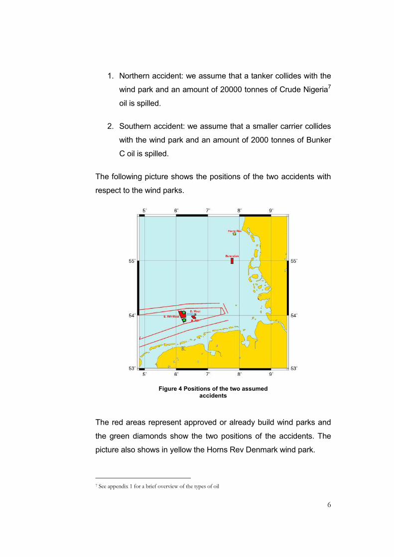
1. Northern accident: we assume that a tanker collides with the
wind park and an amount of 20000 tonnes of Crude Nigeria7
oil is spilled.
2. Southern accident: we assume that a smaller carrier collides
with the wind park and an amount of 2000 tonnes of Bunker
C oil is spilled.
The following picture shows the positions of the two accidents with
respect to the wind parks.
Figure 4 Positions of the two assumed accidents
The red areas represent approved or already build wind parks and
the green diamonds show the two positions of the accidents. The
picture also shows in yellow the Horns Rev Denmark wind park.
7 See appendix 1 for a brief overview of the types of oil

7
We will consider two different types of releases: instantaneous
release (the entire amount of oil is in the water at the moment of
accident) and continuous release (modeled as a succession of 10
instantaneous releases of an equal amount of oil, at one hour
interval, summing up to the total amount of oil).
Different strategies for the cleaning operations are implemented,
like cleaning where the oil slick is thicker or where the mass of oil is
bigger.
The German Wadden Sea coast is divided into 25 ecologically
sensitive zones for which a sensitivity index is known. The following
picture shows these zones, again with respect to the two assumed
positions of accidents.
Figure 5 Sensitivity zones
We mention that the two big boundary boxes 1 and 25 belong to the
coast of Denmark and the Netherlands, respectively.

8
The ecological damages of an oil spill accident are computed and
the results are given for each of these zones. A comparison is made
between the scenario when no response measures are taken and
where mechanical cleaning is performed.
1.3 The fate of spilled oil
The severity of the impact of an oil spill depends on a variety of
factors, including the characteristics of oil itself. We will therefore try
to give a brief overview of the physical properties of oil as well as list
the natural actions that affect it.
The term oil describes a broad range of hydrocarbon-based
substances. Hydrocarbons are chemical compounds composed of
the elements hydrogen and carbon. Some examples are: crude oil,
refined petroleum products, animal fats, and vegetable oils. Each
type of oil has distinct physical and chemical properties. These
properties affect the way oil will spread and break down and the
hazard it may pose to aquatic and human life.
The rate at which oil spill spreads has the biggest weight in the
determination of the effect on the environment. Most oils tend to
spread horizontally into a smooth and slippery surface, called a
slick, on top of the water. The most important factors which affect
the ability of an oil spill to spread are:
1. Surface tension: the measure of attraction between the
surface molecules of a liquid. The higher the oil’s surface
tension, the more likely a spill will remain in place. Because

9
increased temperatures can reduce a liquid’s surface
tension, oil spreads faster in warmer waters
2. Specific gravity: the density of a substance compared to the
density of water. Since most oils are lighter than water, they
float on top of it. However, the specific gravity of oil can
increase when the lighter substances within it evaporate.
Heavier oils can sink and form tar balls or may interact with
rocks or sediments on the bottom of the water
3. Viscosity: the measure of a liquid’s resistance to flow. The
higher the viscosity of oil, the greater the tendency for it to
stay in one place.
In the marine environment natural actions are always working and
can reduce the severity of an oil spill and accelerate the recovery of
an affected area. Such natural processes are generally grouped
under the name weathering: evaporation, oxidation, biodegradation,
and emulsification.
Weathering is a series of chemical and physical changes that can
cause spilled oil to break down and become heavier than water.
Wave, wind and currents may result in natural dispersion breaking a
slick into droplets which are then distributed vertically throughout the
water column.
Evaporation occurs when the lighter or more volatile substances
within the oil mixture become vapors and leave the surface of the
water. This process makes heavier oil, which may undergo further
weathering processes or may sink to the bottom of the water.
10
Oxidation occurs when oxygen combines with the oil hydrocarbons
to produce water-soluble compounds. This process affects oil slicks
mostly at their edges.
Biodegradation occurs when microorganisms feed on oil
hydrocarbons. A wide range of microorganisms is required for a
significant reduction of the oil.
Emulsification is the process that forms emulsion, which are
mixtures of small droplets of oil and water. Such emulsions cause
oil to sink and disappear from the surface, giving the visual illusion
that it is gone and the threat to environment has ended.
1.4 Oil spill response
The only real solution to minimize the environmental and
economical damage that can result from major oil spills lies in
preventing such events happening in the first place. However, once
an oil spill occurred, it is very important to select the appropriate
response.
Knowledge of the type of oil and predictions of its movement are
vital in order to evaluate the impact of the spill. Such an evaluation
can indicate that the oil will remain offshore or will dissipate and
eventually degrade naturally. In this case monitoring the movement
of the slicks to confirm the predictions may be sufficient. However, if
such an evaluation suggests that the oil poses a serious threat to
the environment, the next step is to consider the most adequate
cleanup techniques.

11
The most often used response technique is mechanical response.
It uses physical barriers and mechanical devices to redirect and
remove oil from the water’s surface. Where this technique is
feasible, it is preferable to other methods, since spilled oil is
removed from the environment to be recycled or disposed of
properly. Mechanical removal of oil utilizes two types of equipment:
booms and skimmers. Booms are floating barriers used to redirect
the oil into collection areas or keep it out of the sensitive areas and
to concentrate the oil so that it is thick enough to be skimmed. The
skimmers are the devices that remove oil from the water’s surface.
Their efficiency depends very much on weather conditions.
Non-mechanical methods include dispersants, in situ burning, and
biological response. Dispersing agents are compounds that act to
break the oil into small droplets that disperse into the water column
where they are subject to natural processes that help to break them
down further. This helps to clear the oil from the water surface,
making it less likely to reach the shoreline, but increases the impact
on organisms in the exposed sector of the water column. In-situ
burning means the controlled burning of oil “in place”. Approvals
must be obtained before using this method, since there is a big
concern over atmospheric emission and uncertainty about its impact
on human and environmental health.
1.5 Outline of the thesis
After presenting the background of the project in the first chapter,
we will describe the data used in chapter two. We will briefly give
some facts about the oil-drift model which is the source of data used

12
in our model and we will also describe the weather data necessary
for the simulations.
The third chapter is devoted to the cleaning model. The elements
that build this model and all parameters needed by it are thoroughly
described here.
Chapter four presents the results obtained for various types of
simulations. Different scenarios are considered and the
corresponding results are given.
The next chapter gives an analysis of the results. We make
comparisons between results obtained from different simulations
and explain them. We also try to spot the most important factors
that influence the results and find ways of improving them.
The last chapter gives some final conclusions and
recommendations for further work.
The appendices at the end of the thesis present some information
that was not included in the description of the model and also a part
of the implementations codes.
13
C h a p t e r 2
Description and usage of the data
2.1 The oil-drift model
Computer simulations of dispersion processes have become very
important in the last years, trying to meet the demands of a world
more and more concerned with protecting the environment. Many
applications were developed, including modeling of the dispersion of
pollutants and computations of the drift paths of shipwrecked
persons.
The model used by GKSS to simulate the drift and dispersion of oil
is a Lagrangian dispersion model. The oil is represented by a
particle cloud drifting with the current. The oil floating on the surface
is additionally driven by a certain percentage of wind velocity. In the
simulation of oil dispersion different types of oil are considered with
their particular physical behavior.
The entire amount of oil spilled is represented by a number of
particles of equal mass. We will start by using a number of 1000
particles and later on we will decrease this number to 500 for
computational time reasons.
These particles are followed for 240 hours, at each hour their
location is known as well as the water depth at that location, their
position in the water column and other parameters that might be of
interest. Figures number 6 and 7 show such a cloud of particles at
20 hours and 180 hours after the accident. The particles are color

14
coded: with black are represented the particle that are at the surface
of water, with blue the ones that are at some depth into the water
column and with red the particles that reached the bottom of sea or
the coast.
Figure 6 Oil particles at 20 hours after the moment of accident
15
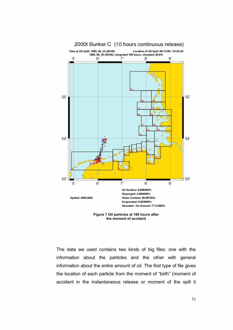
The picture shows also the sensitivity zones and the position of the
simulated accident, represented by a green diamond.
At the bottom of the picture some information on the oil quantities is
given in percentages. We can see that 76.61% of the total amount
of oil spilled is at the surface, 14.26% is dispersed into the water
column, 9.13% is evaporated and 0% is stranded. All these
percentages add up to 100%. We can also see a percentage of
66.33 for the water content, illustrating the fact that in one volume
unit 66.33% is water and only the rest is oil; this is the result of
emulsification.
At 180 hours after the first spill 77.32% is already grounded and
only 9.91% is still at the surface. The water content is of 66.67%,
showing a big decrease in the rate of emulsification since after only
20 hours the water content was already of 66.33%. Also a little more
oil has evaporated, the total percentage reaching now a value of
9.99%.
16
Figure 7 Oil particles at 180 hours after the moment of accident
The data we used contains two kinds of big files: one with the
information about the particles and the other with general
information about the entire amount of oil. The first type of file gives
the location of each particle from the moment of “birth” (moment of
accident in the instantaneous release or moment of the spill it
17
corresponds to, in the continuous release) until it “dies” (the particle
has reached the ground or the simulation ended). Other information
that we will use is the particle’s position in the water column, given
as a number ranging from 1 to 3 (1 if the particle is at surface, 2 if
the particle is at some depth in the water column, and 3 if the
particle has reached the shore or the bottom of the sea). This
information is very important to us since once the oil entered into
the water column it is impossible to clean. We will therefore
consider in our analysis only the particles that are on the surface.
We note here that one particle that is at some depth into the water
column can come again at surface after some period.
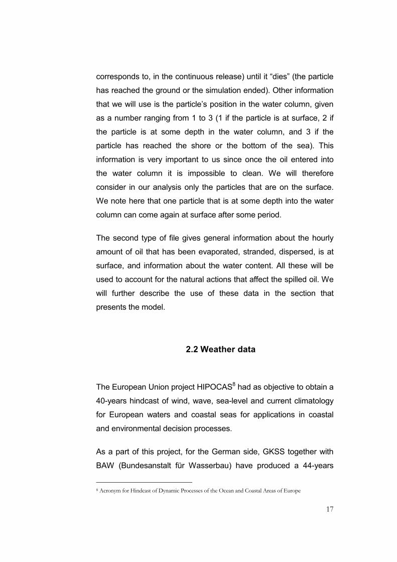
The second type of file gives general information about the hourly
amount of oil that has been evaporated, stranded, dispersed, is at
surface, and information about the water content. All these will be
used to account for the natural actions that affect the spilled oil. We
will further describe the use of these data in the section that
presents the model.
2.2 Weather data
The European Union project HIPOCAS8 had as objective to obtain a
40-years hindcast of wind, wave, sea-level and current climatology
for European waters and coastal seas for applications in coastal
and environmental decision processes.
As a part of this project, for the German side, GKSS together with
BAW (Bundesanstalt für Wasserbau) have produced a 44-years
8 Acronym for Hindcast of Dynamic Processes of the Ocean and Coastal Areas of Europe
18
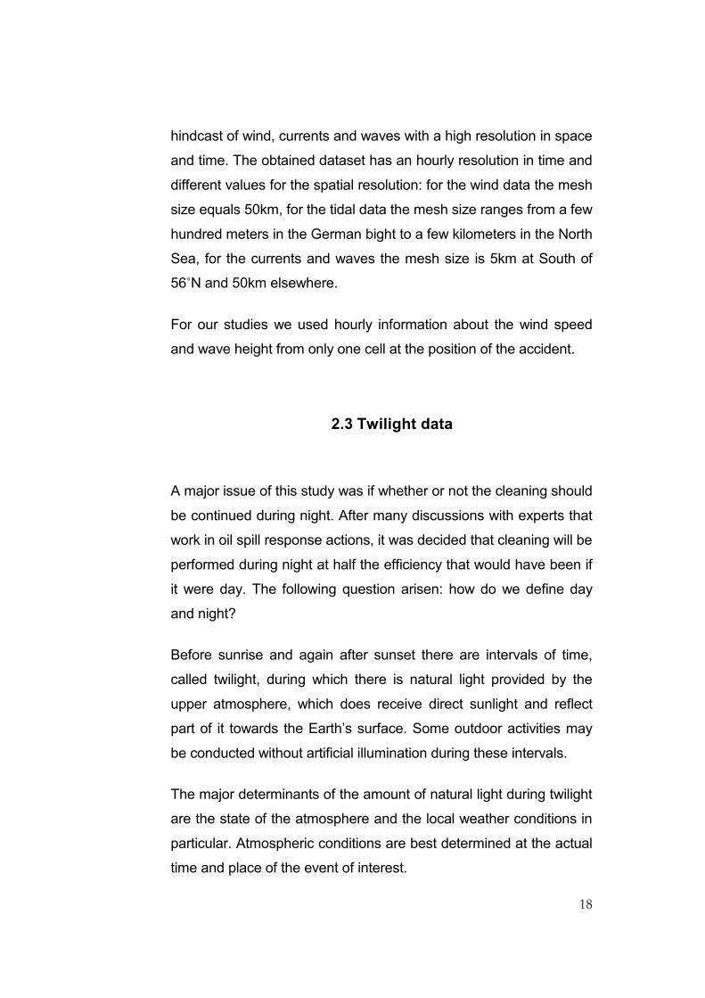
hindcast of wind, currents and waves with a high resolution in space
and time. The obtained dataset has an hourly resolution in time and
different values for the spatial resolution: for the wind data the mesh
size equals 50km, for the tidal data the mesh size ranges from a few
hundred meters in the German bight to a few kilometers in the North
Sea, for the currents and waves the mesh size is 5km at South of
56˚N and 50km elsewhere.
For our studies we used hourly information about the wind speed
and wave height from only one cell at the position of the accident.
2.3 Twilight data
A major issue of this study was if whether or not the cleaning should
be continued during night. After many discussions with experts that
work in oil spill response actions, it was decided that cleaning will be
performed during night at half the efficiency that would have been if
it were day. The following question arisen: how do we define day
and night?
Before sunrise and again after sunset there are intervals of time,
called twilight, during which there is natural light provided by the
upper atmosphere, which does receive direct sunlight and reflect
part of it towards the Earth’s surface. Some outdoor activities may
be conducted without artificial illumination during these intervals.
The major determinants of the amount of natural light during twilight
are the state of the atmosphere and the local weather conditions in
particular. Atmospheric conditions are best determined at the actual
time and place of the event of interest.

19
The nautical twilight, being the one we are interested in, is defined
to begin in the morning and to end in the evening when the center of
the sun is geometrically 12 degrees below the horizon. At the
beginning or end of nautical twilight, under good atmospheric
conditions and in the absence of other illumination, general outlines
of objects may be distinguishable.
There are several free astronomical applications available, which
can give a table with twilight intervals for any year of interest and
any position on the globe. We used different tables for each of the
two accidents. Such a table for the year 1995 and the southern
position of accident is given in appendix 2.
20
C h a p t e r 3
The cleaning model
3.1 Description of the model
Having the data that we presented we can develop a numerical
model to account for the mechanical cleaning in the case of oil spill
accident. The accident we are considering is provoked by the
collision of an oil carrier with the wind park. We will therefore
assume that response vessels are already present at the location of
accident at the moment of the first spill. The cleaning operations will
start immediately. After some period of time, additional vessels will
come from the port. These vessels will come at the place where the
cleaning is performed; therefore the time needed for the vessels to
arrive is computed with respect to that place. Characteristics of the
cleaning vessels and parameters we will use in our model will be
described in a later section. In 24 hours a tanker with unlimited
capacity is available. If the vessels’ storage capacity was reached
until this time, they have to go to an unloading base. Again all the
times involved are computed in the simulation.
As we have already mentioned, the weather plays a very important
role in the cleaning operation. We will incorporate this impact in our
analysis by the use of two parameters: the allowance (a variable
that allows or not the cleaning, depending on the wind speed) and
the efficiency (a variable that will give a percentage out of the
maximum cleaning capacity, based on the wave height).

21
Since we represent the amount of spilled oil by a fixed number of
particles, the characteristics of such a particle need to be
understood. We will assume at the moment of “birth” all particles
have equal mass, defined as the total amount of oil spilled divided
by the number of particles. However, in the case of continuous
release, different particles will belong to different releases; this will
imply that at a certain moment, particles will have different age (the
difference between the current moment and the moment of “birth”).
This is very important to note since newer and older oil behaves
differently and we will try to incorporate this in our model.
All processes affecting the oil, the natural processes already
described as well as the cleaning, will be performed at the particle
level. Cleaning will mean subtracting from the mass of the particle a
quantity computed in such a manner that it accounts for the current
mass and age of the particle.
In the case of continuous release, and even in the instantaneous
release, complicated shapes of the oil slick may appear. We will try
to approach this by assigning a membership to each particle to a
specific class (cluster) after some criterion. This criterion is its
location (the two coordinates: longitude and latitude). We will
explain this in more detail in an ulterior section. At this point we want
to show the advantages of such an approach. The first intuitive
limitation of the success of a cleaning operation is the fast
spreading of the oil: in a very short period of time the oil slick will
cover such a big area that trying to clean the entire area will give
poor results. We will divide this area in smaller areas (the areas of
all particles in the various clusters) and we will choose for cleaning
one such area. Two criteria are implemented for choosing the best

22
cluster, namely the one with the biggest mass and the one with the
biggest thickness.
The mass of a cluster is simply the sum of the masses of its
particles. The possibility of defining a thickness for each cluster is
another advantage of this approach. We will make the assumption
that in such a cluster the particles have equal size (if we think of a
particle as a sphere, this size can be its diameter). Since particles
from a specific cluster have gathered together they must have some
common characteristics, therefore we consider this not to be an
unsatisfactory assumption. Accounting also for the water content,
knowing the mass of the cluster and the oil’s density, we compute
for each cluster its thickness. This property will be also used in the
formula that gives the quantity of oil that can be removed from the
water.
Having all this information, the cleaning model starts by assuming
that a certain accident took place. We will call this an event. The
time step of the simulation is one hour. At each such step, the
particles that are at the water’s surface are considered for the
division in clusters, one such cluster is chosen to be cleaned, the
vessels move to the center9 of the cluster and clean it for the
remaining time (the cleaning time equals one hour minus the time
that was needed to reach the center of that cluster).
The simulation gives as output an hourly quantity of oil removed
from the water, the quantity of oil still at surface as well as the
impact on the 25 sensitivity zones. The impact on one zone can be
seen in the hourly quantity of oil that reached that zone or in the
total amount of oil that was in that zone (counting again the mass of
9 The center of the cluster is the center of mass of the convex hull of that cluster

23
one particle at every moment that it was in that zone, since indeed
that means that it repeatedly affected that zone).
Various results and interpretations for the consequences are given
for one assumed accident. To be able to give some statistics we will
run the model for many accidents. We will consider the period of 10
years, from 1990 until 1999, and assume one accident takes place
at each 28 hours. This will give a total number of 3130 accidents
and we consider it as being sufficiently big number to extract some
patterns from it.
3.2 Characteristics of the cleaning vessels
To model the cleaning procedure, we first need to fix some values
that we will use for the main characteristics of the cleaning vessels.
We assigned these values by averaging over the known parameters
of the spill response vessels used in the European Union countries.
Before listing the parameters used in our model, we will give a brief
description of such a spill response vessel, namely Nordsee:
Figure 8 Nordsee - spill response vessel

24
Nordsee is an oil recovery vessel that uses two sweeping arms
bearing pumps with a suction capacity of 700m3/h each. It
separates oil from water by gravitation and it has a tank to storage
the oil with a capacity of 5400m3. The maximum speed it can reach
is 13knots10. The overall breadth11 of this vessel is 23m.
We have already mentioned that we will assume pre-positioned
vessels at the moment of accident. We will use a number of 5 such
vessels, with identical parameters and we will treat them as one (the
total storage capacity is the sum of all storage capacities, etc.). The
parameters of one such vessel are listed bellow:
storage capacity 1500m3
wing span12 6m
traveling speed 15kn
cleaning speed 1kn
The second formation of vessels that are coming from the port has
also 5 vessels with the same traveling and cleaning speed and with
the following values for the other two parameters:
storage capacity 500m3
wing span 10m
10 1 Knot equals 1 nautical mile per hour or 1.8523 kilometers per hour
11 Breadth, also called beam, is the width of a ship.
12 The wing span is the total length of the sweeping arms

25
3.3 The impact of weather on the cleaning
The mechanical cleaning is impossible when the wind speed is
bigger than 15m/s. To account for this we will introduce a binary
variable, called allowance:
( )≤
= >
wind
wind
wind
1, s 15m / sallowance s
0, s 15m / s
Furthermore, the ability and efficiency of the cleaning depends
greatly on the wave height. If this efficiency is a variable ranging
from 0 to 1, then it will take the maximum value for the wave height
0, and the minimum value for some wave height above which the
mechanical cleaning is impossible. From experts we know that for
wave height bigger than 1.5m the sweeping arms may break and
the decision to continue the cleaning or to stop it is taken by the
captain of the vessel. Finally we received the following values:
Wave height Efficiency 1.5m 40% 0.75m 60% 0.5m 70% 0.25m 90%
We further assume that the efficiency is linearly dependent on the
wave height and the minimum value is taken for a wave height of
2m. This reads:
( ) = ⋅ +wave waveefficiency h a h b
Using the above numbers, we will obtain the following dependence
of the efficiency on the wave height:

26
Figure 9 Efficiency of cleaning
3.4 The clustering technique
An informal definition of clustering could be: the process of
organizing objects into groups whose members are similar in some
way.
We will use a clustering algorithm to define in our set of particles
some groups such that in each of these groups particles are “close”
to each other. During another study (an internship) different types of
algorithms were considered and analyzed and finally one simple
algorithm was chosen. We will first describe its original form13. The
algorithm was developed by Robert Clason14 in 1990.
13 See appendix 3 for the Matlab implementation of this algorithm
14 The algorithm was described in the article “Finding Clusters: An Application of the Distance
Concept” by Robert Clason, April 1990

27
For each cluster there will be a single point that is designated as a
hub15. The placement of the hub within the cluster is determined by
the algorithm. The algorithm will arbitrarily choose one point to be
the first hub and cluster all the points around this hub (all points are
considered to belong to the cluster that has this hub). It then finds
the point farthest away from the hub and makes this point a new
hub. Next it clusters the data around the hub that is nearest (the
points that are closer to the new hub are reassigned to a second
cluster). This process is repeated until the distance16 from every
point to its hub is less than half the average distance between all
pairs of hubs.
We will first illustrate the use of this algorithm on a small dataset
that has just 5 points: A(1,1), B(1,2), C(2,2), D(4,4), E(4,5). The
algorithm starts by designating point A(1,1) as the first hub and
assigning all points to one cluster that has this point as its hub.
The distances between
the first hub and all points
are:
A B C D E
0 1 2 3 2 5
The biggest distance is 5.
This value is compared
with an initial test value,
the second hub. The distances from all points to this new hub are
computed:
15 Centre, kernel (different than the centroid, the hub is one of the points in the dataset); when talking
about distances between cluster we will mean distances between the hubs of the clusters
16 All distances considered in the algorithm are Euclidian distances

28
A B C D E
5 3 2 13 1 0
and compared with the previous distances. Whenever the new
value is smaller it means that the corresponding point should be
assigned to the second hub, forming a second cluster.
To see if a new cluster is
needed we compare two
values:
1. half of the average
distance between all pairs
of hubs, in our case is
simply half of the distance
between A and E, 2.5
2. the maximum distance between each point to its hub.
These distances are:
0 1 2 1 0
2 is smaller than 2.5 and we conclude that no new cluster is
needed.
We could see the stopping condition as a comparison between
inter-cluster distances with between clusters distances. We can see
this better by taking another example, a dataset containing the
previous 5 points and 4 extra. We will show how the points need to
be positioned so that a third cluster is needed. The new dataset
contains now the points A(1,1), B(1,2), C(2,2), D(4,4), E(4,5), F(8,4),
G(9,4), H(8,5), I(9,5). After the first step 2 clusters are formed as
shows the following plot:

29
with hubs A(1,1) and
I(9,5). The biggest
distance between a
point and its hub is 5
(the distance between
points A and E from
the first cluster). Half
the average
distance between hubs is 2 5 . This means that the first cluster
should be further split into two clusters. The final result:
However, if the points
D and E, instead of
having coordinates
(4,4) and (4,5) would
have coordinates (3,4)
and (2,4), the
algorithm would find
only two clusters as
We believe we can
conclude that the
algorithm performs
well. Anyway, things
can still be improved, if
one considers that in a
certain situation the
algorithm should find
more or less clusters. We tried to make some improvements and
the analysis performed to find these improvements will be presented
30
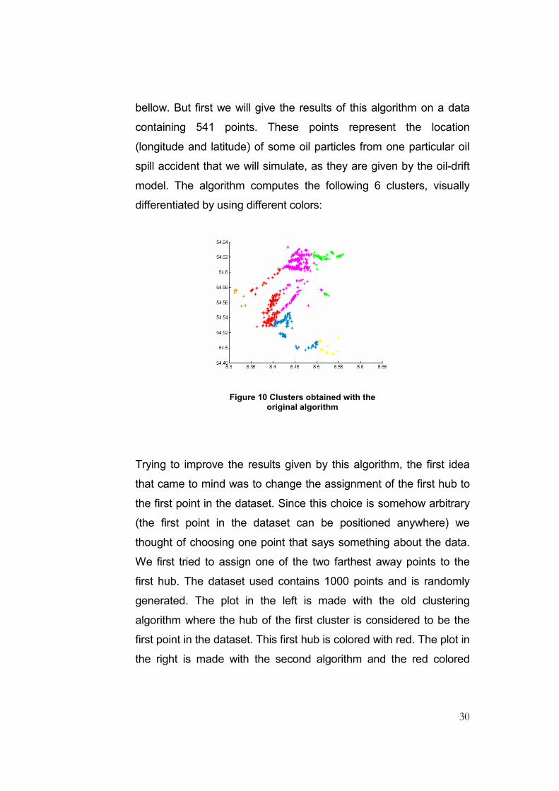
bellow. But first we will give the results of this algorithm on a data
containing 541 points. These points represent the location
(longitude and latitude) of some oil particles from one particular oil
spill accident that we will simulate, as they are given by the oil-drift
model. The algorithm computes the following 6 clusters, visually
differentiated by using different colors:
Figure 10 Clusters obtained with the original algorithm
Trying to improve the results given by this algorithm, the first idea
that came to mind was to change the assignment of the first hub to
the first point in the dataset. Since this choice is somehow arbitrary
(the first point in the dataset can be positioned anywhere) we
thought of choosing one point that says something about the data.
We first tried to assign one of the two farthest away points to the
first hub. The dataset used contains 1000 points and is randomly
generated. The plot in the left is made with the old clustering
algorithm where the hub of the first cluster is considered to be the
first point in the dataset. This first hub is colored with red. The plot in
the right is made with the second algorithm and the red colored

31
point is again the hub of the first cluster, but now being one of the
two farthest away points.
Figure 11 Resulting clusters before and after changing the first hub (1)
Since the hubs of the first two clusters will be the two farthest away
points in the dataset, the new algorithm will split in two or more parts
something that could better be just one single cluster (see the
middle area in the previous plots). We reach the conclusion that this
modification is not suitable for our purposes.
Another idea is to start from one of the points from the densest part
of the dataset. Thus, the modified clustering algorithm computes
first the mean of the data and then finds the closest point in the
dataset to this mean. It then starts clustering from this point. So the
closest point to the mean will be the hub of the first cluster. This will
improve greatly the situation when the data points are somewhat
denser in a specific part of the cloud as you can see from the
following plots. The plot from the left gives the resulting clusters
obtained with the original algorithm and the plot from the right gives
the resulting clusters with the changed limit.

32
Figure 12 Resulting clusters before and after changing the first hub (2)
However, if the dataset does not have this convenient structure and
is for example split in two dense parts, the first algorithm can give
better results. The second algorithm will take the first hub
somewhere in the middle of the two clouds of points and it might not
be able to further separate nicely the points in clusters (since from
this point it can see points in opposite directions as being at the
same distance and therefore puts them in the first cluster, even if
they came from different original clouds). Of course, even the first
algorithm can give a bad result if the first point in the dataset would
be positioned differently. Anyway, for our particular datasets both
situations can appear. We will therefore conclude that such
modifications can be dangerous and try to find other ways of
optimizing the results.
Another option would be to change in the original algorithm the limit
above which a new cluster is made. We have already seen that a
new hub is found if there exists one point that is farther away from
its hub with more than half the average distance from all pair of
hubs. If we change this from half to, let’s say, one third more
clusters will me made and the result will look better. Two
improvements are evident: the points that are kind of outliers are put

33
in separate clusters (maybe they even form clusters of one single
point), and, of course, the cleaning should be better since the area
of the new clusters is smaller. Bellow you can see some examples
obtained with the original limit of 1/2 (left plot) and the new limit of
1/3 (right plot) using some dataset from the model.
Figure 13 Resulting clusters before and after changing the limit to 1/3
Making such plots for various datasets that we will use in the model
and also keeping in mind that for our purpose the obtained clusters
should not be too small, we finally decided to change the limit from
1/2 to 2/5.
Another modification made to the algorithm is also related to the
criteria by which the algorithm decides that a new cluster is needed.
We thought that even if the biggest distance within a cluster is
bigger than the above chosen percentage of 40% from the average-
between-clusters distance, maybe the splitting should not continue if
that biggest distance is smaller than a given value. Again by making
some plots with different values for this limit, knowing also that a
cleaning boat can cover in one hour a distance of one mile (1852m),
we decided to take this limit equal to 500m. So if there is one cluster
with a distance between two points bigger than the average-
between-clusters distance, but this distance is smaller than half a

34
kilometer, the cluster should not be further split (its dimension suits
well our purposes). The result of this final version of the algorithm
for the first randomly generated dataset considered in this section
is:
-40 -30 -20 -10 0 10 20 30 40-40
-30
-20
-10
0
10
20
30
40
Figure 14 Resulting clusters after the final modification
And finally, the result on the dataset of 541 points:
8.3 8.35 8.4 8.45 8.5 8.55 8.6 8.6554.48
54.5
54.52
54.54
54.56
54.58
54.6
54.62
54.64
Figure 15 Clusters obtained with the final algorithm
35
3.5 Incorporating the natural processes
As we have already mentioned, all natural processes that affect the
spilled oil are incorporated into the oil-drift model. As output of this
model is the hourly quantity of oil that has evaporated, dispersed,
stranded, and is at surface, as well as the water content. All this
information is given as a percentage of the quantity of oil spilled.
Our task remains just to use these values properly.
At the beginning of each hour in our simulation we first treat the
evaporation. We subtract from the mass of all particles that are at
the water surface an amount proportional to their mass from the
total mass that has evaporated in the previous hour (the value given
by the oil-drift model). Just afterwards we apply the cleaning, but
only to the particles from the chosen cluster. The other information
about the stranded, dispersed and at surface quantities we will use
just for verifications at the end of each simulation (check if the sum
of the total quantity cleaned, the total quantity that has evaporated,
the total quantity stranded, and the total quantity dispersed equals
the total quantity of spilled oil). We do not use this information
because it is already incorporated, just in a different manner: at
each hour of our simulation we work only with the particles that are
at surface of water at that hour, we do not include particles that are
at some depth into the water column or are already aground.
We will use the information about the water content to compute the
volume of the chosen cluster. Afterwards we will use this volume to
compute the thickness of the cluster. This value is given as a
percentage out of the oil volume. We first get the percentage that
should correspond only to the cluster (what we have is the hourly

36
water content of the entire current quantity of oil). We then have the
following relationship:
= + *cluster oil clusterVolume Volume p Volume ,
where p is the above percentage. We finally have:
ρ= =
− −
1*
1 1
oil oil
cluster
oil
Volume MassVolume
p p,
where ρoil is the density of oil and oilMass is the mass of the cluster
(the sum of the masses of the oil particles in the cluster).
We can compute now the cluster’s thickness as being the ratio
between the cluster’s volume and the cluster’s area.
3.6 The quantity of oil hourly removed
We finally arrive at the formula that gives the quantity of oil that can
be hourly removed from the water’s surface.
We need to define one more variable: the covered area. This is the
area that can be covered by the formation of vessels in the time that
it has for the cleaning. That means simply:
=
−
* *
(1 )
AreaCovered Wing Span of the formation Speed of the formation
Time needed to reach the cluster
Multiplying this value with the cluster’s thickness we obviously
obtain the volume covered. But the obtained volume is the volume
of the mixture of oil and water. What we need is just the quantity of

37
oil that can be removed. We therefore find the mass of oil per
volume unit by:
=Mass cluster
Mass of oil per volume unitVolume cluster
(this quantity represents indeed just oil since the mass of cluster is
the mass of oil).
Multiplying the above value with the volume covered we obtain the
mass of oil that can be removed. All the above can be seen in the
picture bellow:
Figure 16 Cleaning formula
We need to incorporate also the impact of weather: the allowance
and the efficiency. We have also mentioned that during night the
cleaning operations are assumed to be half as efficient; we model
this with a variable multiple:

38
∈=
∈
1,
0.5,
hour day timemultiple
hour night time
The formula used to compute the quantity that is removed from the
water at some particular hour is:
= * * *
* *
Mass clusterQuantity of cleaned oil Area covered Thickness cluster
Volume cluster
allowance efficiency multiple
We will give now a sketch of the steps of a simulation for one event
(the quantity of spilled oil of 2000 tonnes is represented by 1000
particles followed for 240 hours; we consider a continuous release
modeled as 10 successive releases of 200 tonnes):
Figure 17 Sketch of the model

39
C h a p t e r 4
Display and examination of the results
4.1 First simulations – year 1995
4.1.1 Continuous release
The first data set that we worked with is composed of all events in
the year 1995. There are 313 events, starting on 1st of January,
hour 16:00, with a time step of 28 hours, ending on 31st of
December, hour 16:00. As we already mentioned, we will start by
representing the quantity of spilled oil by a number of 1000
particles. The oil-drift model gives us the positions of the particles
for 240 hours (10 days). All accidents considered are southern
accidents. We will first simulate a continuous release. For
comparison, the next sub-section presents the results obtained
when we simulate an instantaneous release.
All parameters needed by the model were already described. We
will begin by presenting the results of the simulations. We will
choose a cluster to clean, based on the thickness. Since the time
remaining to clean the chosen cluster is also important, instead of
choosing the cluster that has the biggest thickness, we will choose
the one that has the biggest value of the product
thickness*timeToCleanTheCluster. Doing so we will avoid the
situation when a very thick cluster is chosen to be cleaned, but
being so far from the current locations of the cleaning vessels, it will

40
be cleaned for a very short period of time. We consider that in such
situation, the cleaning will be more efficient if a thinner but closer
cluster is chosen.
The next two tables present the best and the worst event, from the
point of view of the efficiency of cleaning. We mention here again
that the oil spilled in a southern accident is of the type Bunker C,
which is heavy oil. Such oil evaporates at most 30%. The oil-drift
model considers a maximum value of 10 for the percentage of oil
that evaporates: in 240 hours about 9.97% from the total quantity of
spilled oil evaporates. All quantities presented from now on will be
given in tonnes, unless otherwise specified.
Event 1995 / 07 / 29 / 12
Quantity of oil removed 1445.970
Quantity of oil evaporated 201.280
Quantity of oil still at surface after 10 days
72.020
Event 1995 / 03 / 17 / 08
Quantity of oil removed 0.177
Quantity of oil evaporated 199.100
Quantity of oil still at surface after 10 days
140.225
In the best case almost 75% of the total quantity of spilled oil is
removed from the water’s surface in the first 10 days. This is of
course mainly due to the good weather. We will give the plots in
time of the quantity of oil removed and the efficiency.

41
Figure 18 Cleaned oil, 1995072912
Figure 19 Efficiency, 1995072912
In the worst case less than 0.01% of the quantity of spilled oil is
removed. The cleaned quantity equals zero for a long period of
time, on the background of an efficiency also zero:

42
Figure 20 Cleaned oil, 1995031708
Figure 21 Efficiency, 1995031708
These plots were given to briefly present the best and worst events
in the year 1995. A more thorough analysis of the limitations of the
cleaning operations will be made in a later chapter.
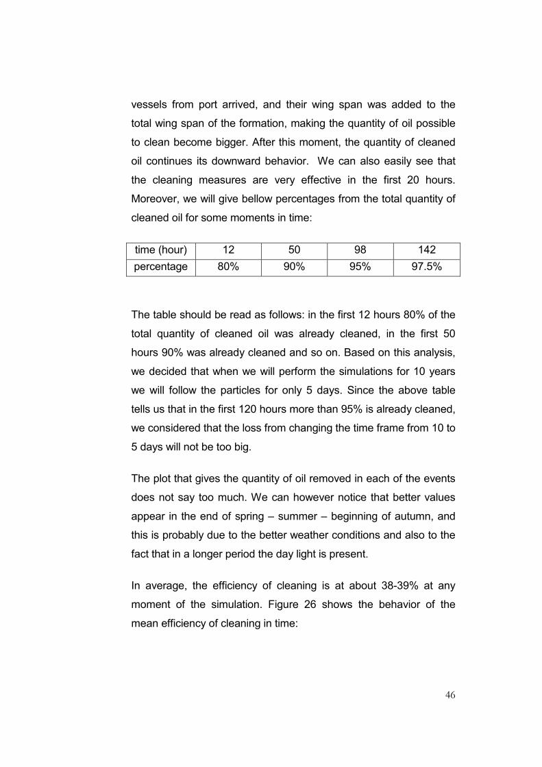
We will present now the consequences of these two accidents on
the environment. The plots will show the total amount of oil that

43
affected in the period of 10 days each of the 25 sensitivity zones. In
the event when the biggest quantity of oil is removed, the most
affected zone is zone one from the border with The Netherlands. In
the event when the smallest quantity of oil is removed, other zones
are affected.
Figure 22 Consequences, 1995072912

44
Figure 23 Consequences, 1995031708
We will now give the overall results obtained using all 313 events
from the year 1995. The following table gives the mean and
standard deviation of the quantity of oil removed from the water’s
surface, the evaporated quantity, and the quantity of oil still at
surface.
Mean Std
Quantity of oil removed
536.400 385.440
Quantity of oil evaporated
200.316 0.784
Quantity of oil still at surface after 10 days
368.924 258.823
45
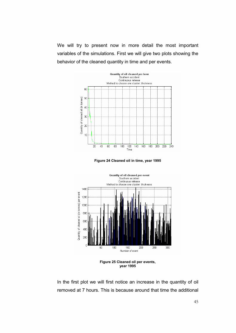
We will try to present now in more detail the most important
variables of the simulations. First we will give two plots showing the
behavior of the cleaned quantity in time and per events.
Figure 24 Cleaned oil in time, year 1995
Figure 25 Cleaned oil per events, year 1995
In the first plot we will first notice an increase in the quantity of oil
removed at 7 hours. This is because around that time the additional
46
vessels from port arrived, and their wing span was added to the
total wing span of the formation, making the quantity of oil possible
to clean become bigger. After this moment, the quantity of cleaned
oil continues its downward behavior. We can also easily see that
the cleaning measures are very effective in the first 20 hours.
Moreover, we will give bellow percentages from the total quantity of
cleaned oil for some moments in time:
time (hour) 12 50 98 142
percentage 80% 90% 95% 97.5%
The table should be read as follows: in the first 12 hours 80% of the
total quantity of cleaned oil was already cleaned, in the first 50
hours 90% was already cleaned and so on. Based on this analysis,
we decided that when we will perform the simulations for 10 years
we will follow the particles for only 5 days. Since the above table
tells us that in the first 120 hours more than 95% is already cleaned,
we considered that the loss from changing the time frame from 10 to
5 days will not be too big.
The plot that gives the quantity of oil removed in each of the events
does not say too much. We can however notice that better values
appear in the end of spring – summer – beginning of autumn, and
this is probably due to the better weather conditions and also to the
fact that in a longer period the day light is present.
In average, the efficiency of cleaning is at about 38-39% at any
moment of the simulation. Figure 26 shows the behavior of the
mean efficiency of cleaning in time:

47
Figure 26 Efficiency, year 1995
Figures 27 to 30 will give the mean characteristics of the chosen
cluster in time: its mass, area, volume, and thickness. Of course,
even if no cleaning is possible because of the weather conditions,
one cluster is chosen and the cleaning vessels go to that cluster. So
these characteristics exist for each moment of the simulation,
independent of the ability or efficiency of cleaning.

48
Figure 27 Mass of the chosen cluster (1), year 1995
Figure 28 Area of the chosen cluster (1), year 1995

49
Figure 29 Volume of the chosen cluster (1), year 1995
Figure 30 Thickness of the chosen cluster (1), year 1995
We will present now the consequences of these accidents on the
environment. The following plots show the mean total quantity of oil
that reached each of the sensitivity zones in a period of 10 days
after the moment of accident and the total mass of oil affecting the
environment (all 25 zones) per event. We can notice here the most

50
important difference that will appear with the results of the
simulations for only 5 days. The plots presented here can be
compared later on with the corresponding ones obtained for the
entire period of 10 years, when simulating only for 5 days. Even if
the total quantity cleaned is almost equal when the cleaning is
carried on for 10 days, the effects of the spill on the environment are
more severe. More zones are affected, the oil reaching in 10 days
even zones that it did not reach in the first 5 days. Also the
quantities are bigger, since oil particles repeatedly attack the
sensitivity zones.
Figure 31 Consequences (1), year 1995

51
Figure 32 Consequences (2), year 1995
Figure 33 Consequences (3), year 1995
The most affected is zone 1 and the least affected is zone 16. The
gradual effect of the spill in time on those two zones is presented in

52
figures 34 and 35. In the most affected zone in a time interval of one
hour even a mean mass of over 90 tonnes can exist, whereas the
least affected zone has a mean mass of oil of 5 kilograms at the end
of these 10 days.
Figure 34 Consequences (4): most affected zone, year 1995
Figure 35 Consequences (5): least affected zone, year 1995

53
We will now present the impact of the same accidents when no
cleaning measures are performed. In this way we can see to which
extent the response measure chosen protects the environment.
Figure 36 Consequences (6), year 1995
Figure 37 Consequences (7), year 1995

54
The amounts of oil that affect each of the 25 zones are somewhat
bigger. As a comparison: the most affected zone when no cleaning
is performed is attacked by a mean quantity of over 20000 tonnes,
while when cleaning measures are taken, it is attacked by 12000
tonnes.
Figure 38 gives the mass of oil affecting the environment in each of
the 313 events. It has the same shape as the corresponding one
when cleaning measures are taken (figure 32). However, we can
distinguish between events when the cleaning was and was not
efficient. For example in the first 50 events the same values appear
in both plots, suggesting that cleaning was not effective at all, while
around the 200th event the values are quite different, showing that
the cleaning measures helped protecting the environment.
Figure 38 Consequences (8), year 1995
In time the quantity of oil that reaches the most affected zone is also
much bigger than when cleaning is performed. A maximum amount
of over 150 tonnes oil can be in this zone in one hour, compared

55
with a maximum of 90 tonnes when cleaning is performed (see
figure 34).
Figure 39 Consequences (9): most affected zone, year 1995
4.1.2 Instantaneous release
In the simulations for an instantaneous release the entire amount of
oil spilled is assumed to be in the water at the moment of accident.
The main difference with the results from the simulations of
continuous releases will be related to the quantity of oil removed in
the first 10 hours. Since for the instantaneous release in the first 10
hours a bigger quantity of oil exists at the water’s surface, also the
quantity of oil that can be cleaned will be bigger. Since the results
presented for the simulation of continuous releases are many, we
will try to give here just the most important corresponding ones, for
comparison.

56
The event when the biggest quantity of oil is removed has changed
to 1995/05/04/04, while the one when the smallest quantity of oil is
removed remained the same.
Quantity of oil removed
1995 / 05 / 04 / 04 1709.050
1995 / 03 / 17 / 08 0.279
The plots in time of the quantities of oil removed in the two
accidents are presented bellow. In the best scenario 1400 tonnes
out of the total of 1700 are removed in the first hour (the entire
amount of oil is in the water at the first hour, it is concentrated,
giving the possibility of choosing for cleaning a cluster with a big
mass). More than 80% is removed in the first hour; in the
continuous case an equal percentage is removed gradually in the
first 12 hours (see figure 18). In the worst scenario, since almost no
oil is removed, figure 41 bellow is very similar to figure 20 obtained
when continuous release is simulated.
Figure 40 Cleaned oil, 1995050404

57
Figure 41 Cleaned oil, 1995031708
The next two plots show the impact of these two accidents on the
environment. Comparing figures 42 and 22, we can notice that even
if an almost equal quantity of oil is removed in the best scenario, still
the consequences are much lower when an instantaneous release
is assumed. This is a result of what was mentioned earlier: the most
part of oil is removed in the first hour and much less oil remains to
reach the sensitivity zones. In the worst scenario the consequences
are similar, only that different sensitivity zones are affected. To see
this we can compare figure 43 with figure 23.
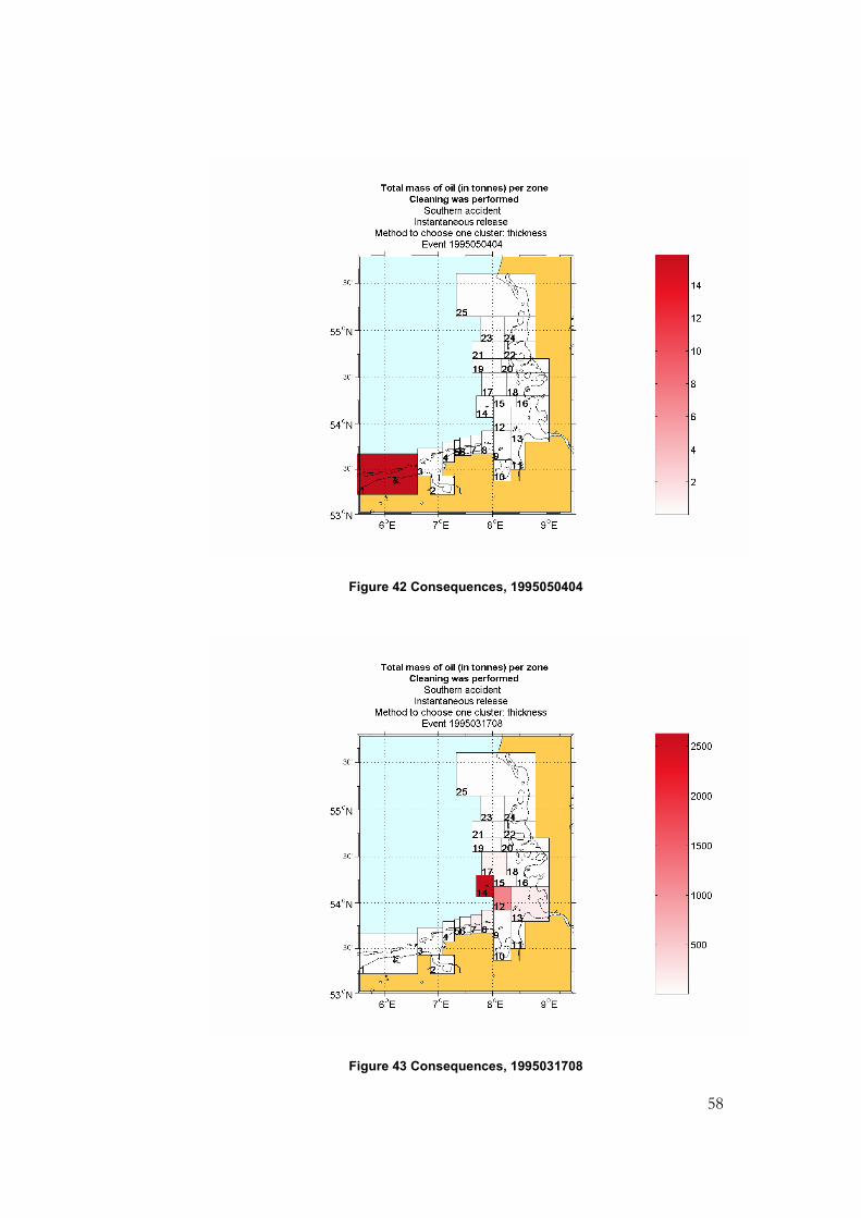
58
Figure 42 Consequences, 1995050404
Figure 43 Consequences, 1995031708

59
We will present now the overall results. The next table contains the
means and standard deviations for the quantities of removed,
evaporated, and still at surface oil.
Mean Std
Quantity of oil removed
622.660 452.429
Quantity of oil evaporated
199.764 0.667
Quantity of oil still at surface after 10 days
560.725 266.087
The same main difference that appeared for the best scenario is still
valid for the overall results: in the first hour a much bigger quantity
of oil is removed. Also the same increase is visible at about 7 hours
when the additional vessels from port add to the cleaning formation.
Figure 44 Cleaned oil in time, year 1995
Per events, the plot of the total quantity of oil removed looks similar
to the plot obtained when simulating a continuous release (figure
25), only the quantities are somewhat bigger.

60
Figure 45 Cleaned oil per events, year 1995
For comparison, the next plots show mean characteristics of the
chosen cluster in time. We can note that the quantities follow the
same pattern as in figures 27-30. The masses of the clusters
chosen in the first hours are obviously bigger. Also the thickness of
the chosen cluster in the first hour is much bigger than the one
obtained in a continuous release. This is because a very big amount
of oil is in the water at the first hour of accident. The positions of the
oil particles, as output of the oil-drift model, are very close to each
other. As a consequence, a big mass of oil is concentrated in a
small area, giving a thickness of the oil slick unrealistically big. More
about this will be discussed when presenting the results of the
simulations for a larger period of time.

61
Figure 46 Mass of the chosen cluster (2), year 1995
Figure 47 Area of the chosen cluster (2), year 1995

62
Figure 48 Volume of the chosen cluster (1), year 1995
Figure 49 Thickness of the chosen cluster (1), year 1995
The consequences on the environment are presented bellow. The
total mass of oil affecting the environment is smaller, from the same
reasons discussed for the best scenario.

63
Figure 50 Consequences (10), year 1995
Figure 51 Consequences (11), year 1995

64
Figure 52 Consequences (12), year 1995
The most affected zone on average is still zone 1, however in this
case with a maximum mass of 25 tonnes in one hour. No oil particle
reaches zone 10 in the 10 days time frame.
Figure 53 Consequences (13): most affected zone, year 1995

65
When no cleaning operations are performed, the environment is
affected as follows:
Figure 54 Consequences (14), year 1995
Figure 55 Consequences (15), year 1995

66
Figure 56 Consequences (16), year 1995
Zone 1 has a maximum amount of oil of 45 tonnes in one hour
interval compared with the maximum of 25 tonnes that can be
observed in figure 53.
Figure 57 Consequences (17): most affected zone, year 1995

67
4.2 Simulations for the period 1990-1999
The simulations for the period of ten years are made on a time
frame of only 5 days for the reasons already explained. To save
more computational time another change is made: the amount of
spilled oil will be represented by 500 particles instead of 1000.
More scenarios will be considered this time. Accidents starting on
both assumed positions are simulated. We will also distinguish
between choosing one cluster to be cleaned based on its thickness
or on its mass. The following scheme gives all possible types of
simulations, presenting the corresponding combinations of
scenario’s parameters:
For the period 1990-1999 we simulated only continuous releases
because we consider that modeling an oil spill accident by a
continuous release is more realistic and also because of the time
limitation. We will therefore give results for 4 types of simulation,
differentiated by the place of the accidents that are simulated and
by the choice of the cluster to be cleaned.

68
4.2.1 Southern accident. Method to choose one cluster:
thickness
We will present the overall results obtained from the simulation of
3126 events in the time interval 1990 -1999. The following table
gives some statistics for the total quantity of oil removed from the
water’s surface.
Total quantity of oil removed
Mean 579.298
Std 389.713
Max 1625.357 1993 / 11 / 26 / 08
Min 0.000
19 events starting in one of the months:
01, 03, 09, 10, 11, 12
We can note that in average about a quarter of the spilled quantity
of oil is removed during the first 5 days of mechanical cleaning.
However, some help is added by the type of oil considered: it is
heavy oil, so it evaporates slowly and therefore the cleaning is more
effective. This will be better seen when the results for the northern
accident are presented, where lighter oil is assumed to be spilled.
We can further notice that even as much as 80% of the total
quantity of spilled oil can be removed in the first 5 days. Again, we
need to mention that the simulated spill is a small one, in reality
accidents when as much as 120,000 tonnes can be spilled. The
events when no oil is removed are triggered by very bad weather
and therefore efficiency of cleaning equal to 0 for the entire period of
simulation. Since we only use the weather from only one cell,
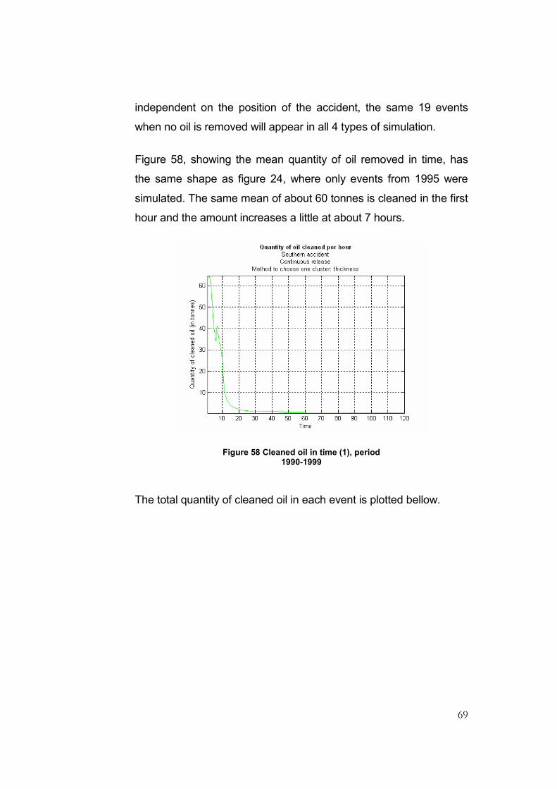
69
independent on the position of the accident, the same 19 events
when no oil is removed will appear in all 4 types of simulation.
Figure 58, showing the mean quantity of oil removed in time, has
the same shape as figure 24, where only events from 1995 were
simulated. The same mean of about 60 tonnes is cleaned in the first
hour and the amount increases a little at about 7 hours.
Figure 58 Cleaned oil in time (1), period 1990-1999
The total quantity of cleaned oil in each event is plotted bellow.

70
Figure 59 Cleaned oil per events (1), period 1990-1999
The mean efficiency in time takes values a little bigger than the
ones that can be observed in figure 26, showing that the year 1995
had a worse weather than the mean. The curves are also smoother
and more regular, more events being considered in this simulation.
Figure 60 Efficiency, period 1990-1999

71
The plots bellow show mean characteristics of the cluster that is
chosen to be cleaned. Expected patterns as a continuous increase
of the area are visible. The mass of the chosen cluster also
increases in the first 10 hours since the oil is spilled gradually and
than starts oscillating.
Figure 61 Mass of the chosen cluster (1), period 1990-1999
Figure 62 Area of the chosen cluster (1), period 1990-1999

72
The volume of the chosen cluster follows almost the same pattern
as the mass, increasing in the first hours and than slowly
decreasing.
Figure 63 Volume of the chosen cluster (1), period 1990-1999
A very important remark needs to be made here. Occasionally, very
big values of the thickness can appear because the area of the
cluster is close to zero. When a spill is simulated by the oil-drift
model, the resulting particles can be very close to each other. The
cleaning model can choose the cluster formed by only the particles
from the current spill, since that cluster will have a big mass and
also a big thickness. However, its area will be very small and
therefore the computed thickness can reach unrealistic values. In
waters of depth around 40 meters, thickness of kilometers can
appear. Neglecting this strange situation, an expected decreasing of
the thickness can be noticed, on a background of a slowly
decreasing volume after the first hours and an increasing area.

73
Figure 64 Thickness of the chosen cluster (1), period 1990-1999
We will give here the plot in time of the mean period that a cluster is
cleaned. All values are over 55 minutes, showing that the cleaning
vessels do not lose much time moving from one cluster to another.
This is a very important remark since the vessels are assumed not
to clean while moving from one cluster to another (this was a natural
assumption based of the very big difference between the cleaning
and the traveling speed of the vessels – the traveling speed is 15
times bigger than the cleaning speed). We will omit the
corresponding plots in the other types of simulation, since they all
look the same.

74
Figure 65 Time to clean the chosen cluster, period 1990-1999
The mean consequences of these accidents on the sensitivity
zones are given bellow. To make more visible the differences of
performing cleaning operations versus not performing, we will
couple the two types of plots. All parameters of the simulations
appear in the pictures’ titles.

75
Figure 66 Consequences (18), period 1990-1999
Figure 67 Consequences (19), period 1990-1999

76
Figure 68 Consequences (20), period 1990-1999
Figure 69 Consequences (21), period 1990-1999
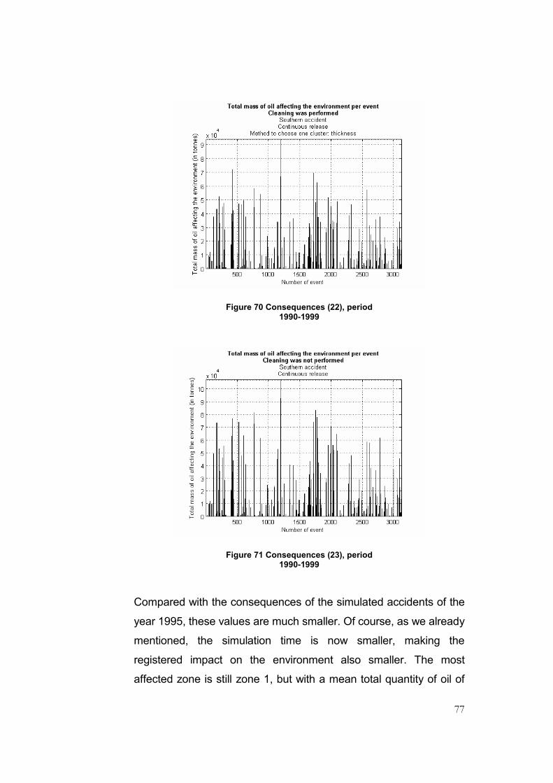
77
Figure 70 Consequences (22), period 1990-1999
Figure 71 Consequences (23), period 1990-1999
Compared with the consequences of the simulated accidents of the
year 1995, these values are much smaller. Of course, as we already
mentioned, the simulation time is now smaller, making the
registered impact on the environment also smaller. The most
affected zone is still zone 1, but with a mean total quantity of oil of
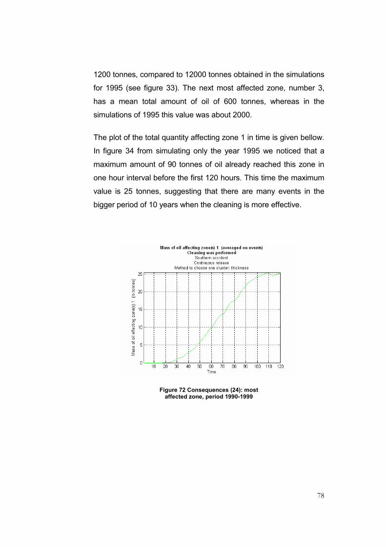
78
1200 tonnes, compared to 12000 tonnes obtained in the simulations
for 1995 (see figure 33). The next most affected zone, number 3,
has a mean total amount of oil of 600 tonnes, whereas in the
simulations of 1995 this value was about 2000.
The plot of the total quantity affecting zone 1 in time is given bellow.
In figure 34 from simulating only the year 1995 we noticed that a
maximum amount of 90 tonnes of oil already reached this zone in
one hour interval before the first 120 hours. This time the maximum
value is 25 tonnes, suggesting that there are many events in the
bigger period of 10 years when the cleaning is more effective.
Figure 72 Consequences (24): most affected zone, period 1990-1999
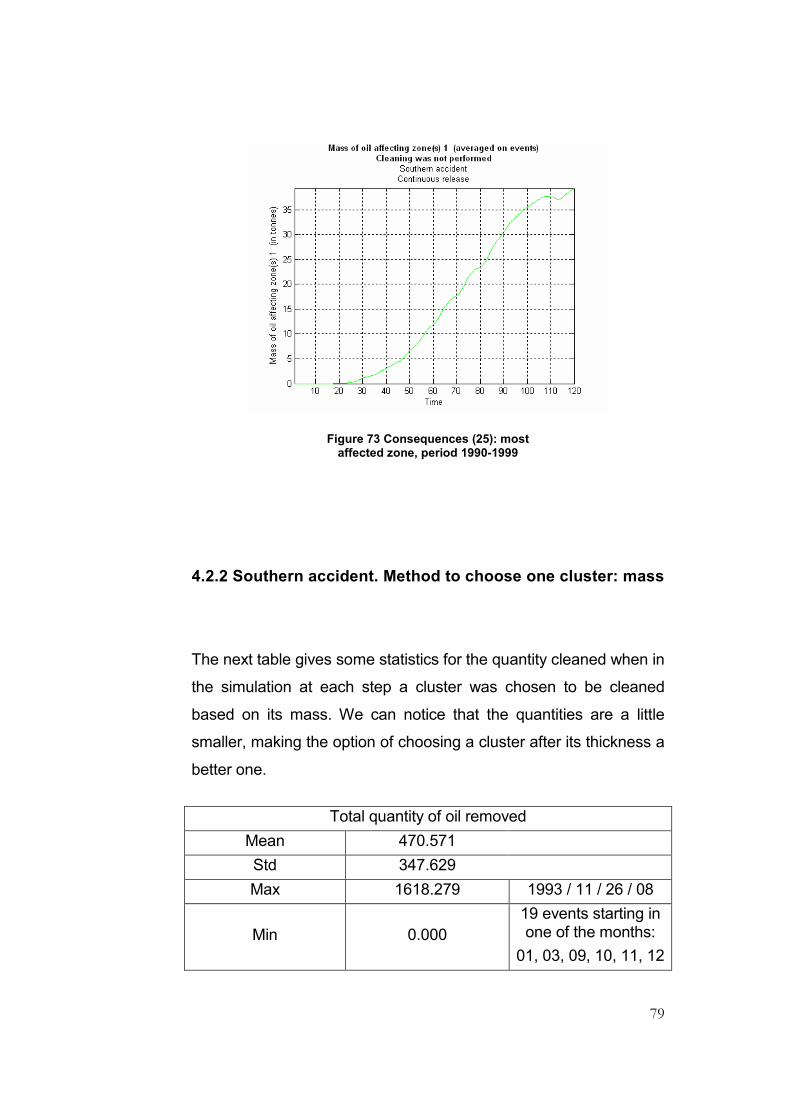
79
Figure 73 Consequences (25): most affected zone, period 1990-1999
4.2.2 Southern accident. Method to choose one cluster: mass
The next table gives some statistics for the quantity cleaned when in
the simulation at each step a cluster was chosen to be cleaned
based on its mass. We can notice that the quantities are a little
smaller, making the option of choosing a cluster after its thickness a
better one.
Total quantity of oil removed
Mean 470.571
Std 347.629
Max 1618.279 1993 / 11 / 26 / 08
Min 0.000
19 events starting in one of the months:
01, 03, 09, 10, 11, 12

80
The plot in time of the mean total quantity of oil removed looks very
similar to the one obtained with the other method of choosing one
cluster (figure 58), just the values are smaller.
Figure 74 Cleaned oil in time (2), period 1990-1999
The total cleaned quantity per event is plotted bellow.
Figure 75 Cleaned oil per events (2), period 1990-1999

81
The next plots present some characteristics of the chosen cluster.
Some differences with the corresponding plots from the previous
sub-section are visible. First of all, comparing figure 61 with figure
76, we can notice that the mass of the chosen cluster is bigger. This
was expected since the new method tries to choose the heaviest
cluster. The area of the chosen cluster is also bigger in this case
and this is also understandable because choosing the thickest
cluster means indirectly choosing a cluster with a smaller area.
Therefore the previous method was trying to find clusters where the
particles are more crowded, while the new method can look for
clusters where a big mass exist on a large area.
Figure 76 Mass of the chosen cluster (2), period 1990-1999

82
Figure 77 Area of the chosen cluster (2), period 1990-1999
Figure 78 showing the volume of the chosen cluster is similar with
figure 63, only with somewhat bigger values by the same reason
given above.
Figure 78 Volume of the chosen cluster (2), period 1990-1999
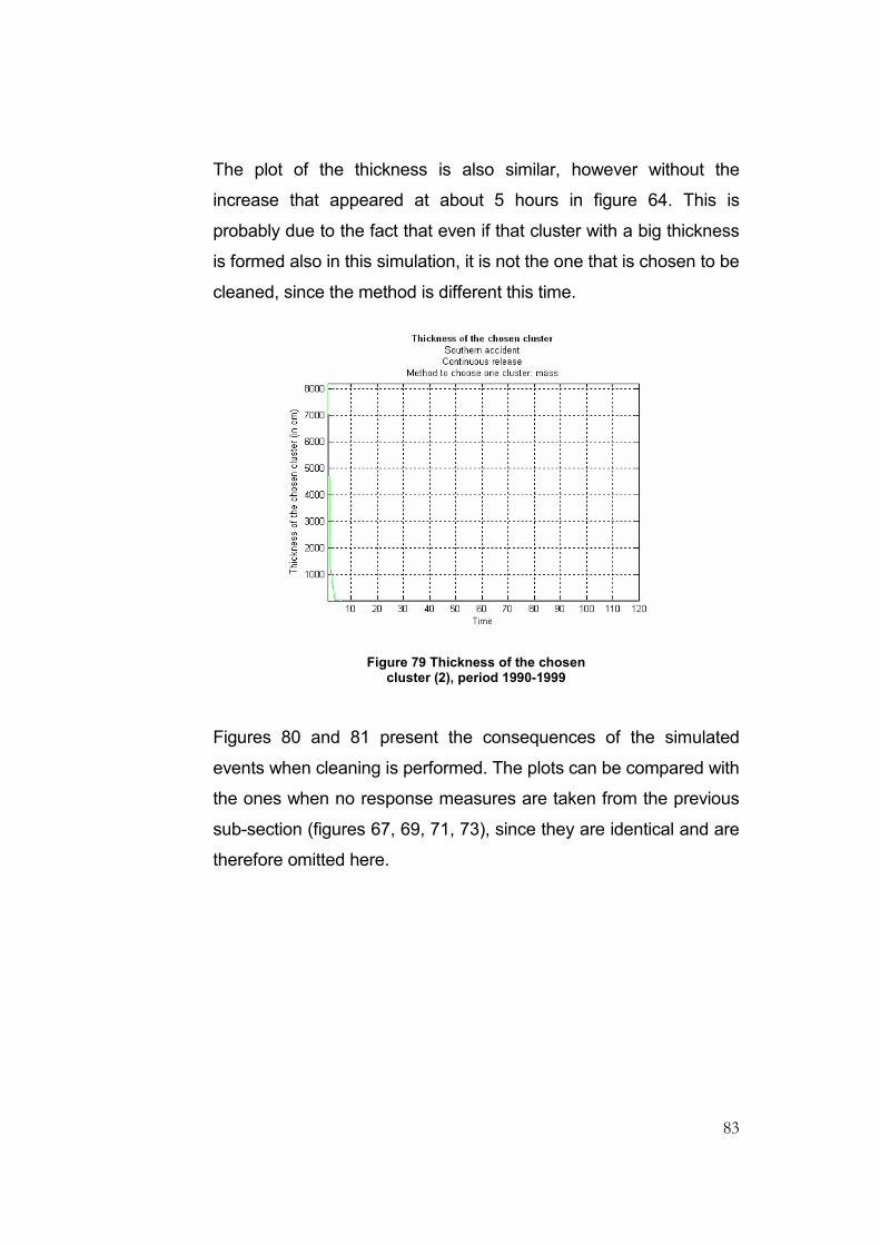
83
The plot of the thickness is also similar, however without the
increase that appeared at about 5 hours in figure 64. This is
probably due to the fact that even if that cluster with a big thickness
is formed also in this simulation, it is not the one that is chosen to be
cleaned, since the method is different this time.
Figure 79 Thickness of the chosen cluster (2), period 1990-1999
Figures 80 and 81 present the consequences of the simulated
events when cleaning is performed. The plots can be compared with
the ones when no response measures are taken from the previous
sub-section (figures 67, 69, 71, 73), since they are identical and are
therefore omitted here.
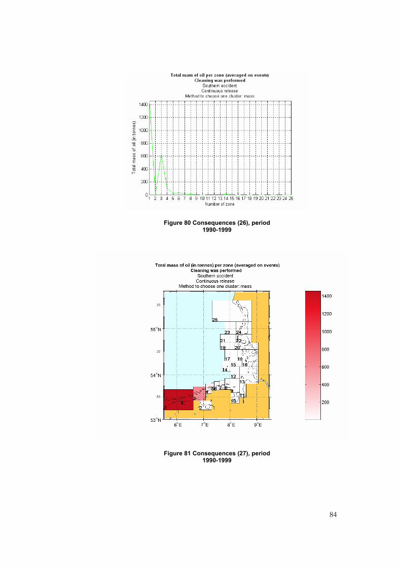
84
Figure 80 Consequences (26), period 1990-1999
Figure 81 Consequences (27), period 1990-1999
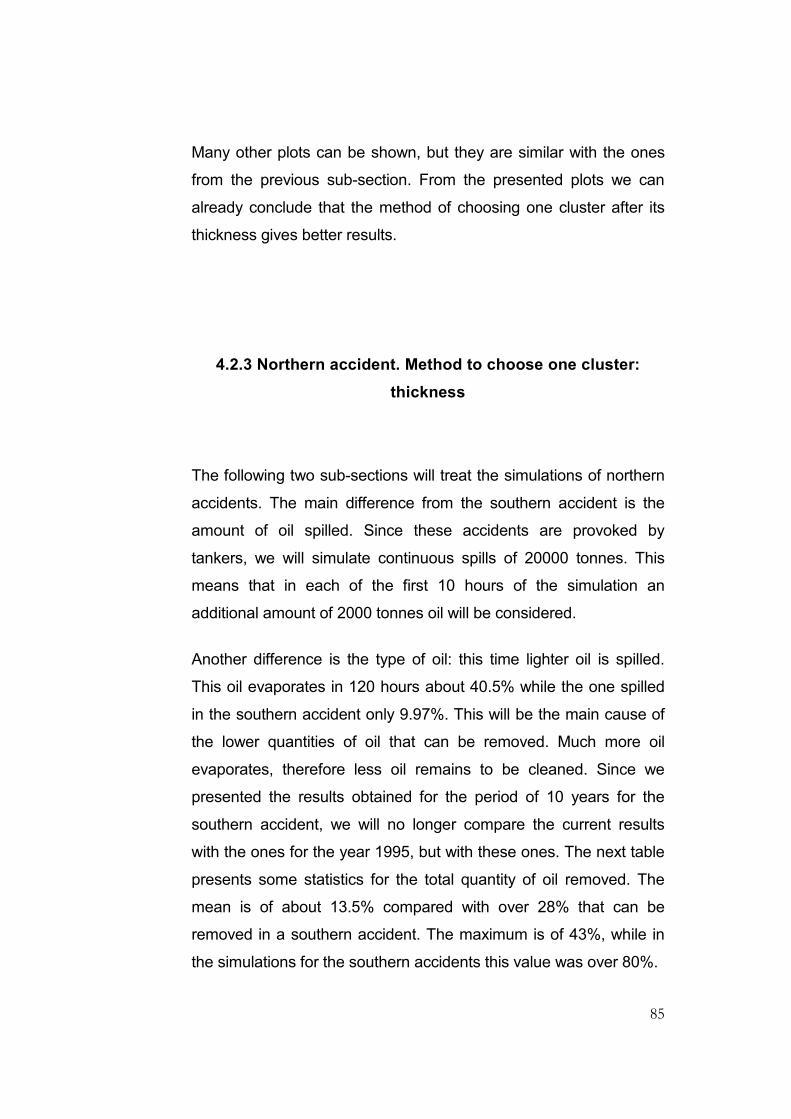
85
Many other plots can be shown, but they are similar with the ones
from the previous sub-section. From the presented plots we can
already conclude that the method of choosing one cluster after its
thickness gives better results.
4.2.3 Northern accident. Method to choose one cluster:
thickness
The following two sub-sections will treat the simulations of northern
accidents. The main difference from the southern accident is the
amount of oil spilled. Since these accidents are provoked by
tankers, we will simulate continuous spills of 20000 tonnes. This
means that in each of the first 10 hours of the simulation an
additional amount of 2000 tonnes oil will be considered.
Another difference is the type of oil: this time lighter oil is spilled.
This oil evaporates in 120 hours about 40.5% while the one spilled
in the southern accident only 9.97%. This will be the main cause of
the lower quantities of oil that can be removed. Much more oil
evaporates, therefore less oil remains to be cleaned. Since we
presented the results obtained for the period of 10 years for the
southern accident, we will no longer compare the current results
with the ones for the year 1995, but with these ones. The next table
presents some statistics for the total quantity of oil removed. The
mean is of about 13.5% compared with over 28% that can be
removed in a southern accident. The maximum is of 43%, while in
the simulations for the southern accidents this value was over 80%.

86
Total quantity of oil removed
Mean 2738.465
Std 1944.495
Max 8619.620 1990 / 05 / 05 / 12
Min 0.000
19 events starting in one of the months:
01, 03, 09, 10, 11, 12
In time, the plot of the mean quantity of oil removed is:
Figure 82 Cleaned oil in time (3), period 1990-1999
In the first hour a mean quantity of about 300 tonnes of oil is
removed. This is in fact a very nice result since it can be compared
with the quantity of oil cleaned in an instantaneous release from a
southern accident (figure 44). The first release in a northern
accident is of 2000 tonnes, equal to the total amount of oil that is
spilled in a southern accident. That makes that at the first hour after
the accident the same amount of oil exists in water in a continuous
release in a northern accident and in an instantaneous release in a

87
southern accident. Figure 44 showing the behavior in time of the
mean quantity of oil removed in the simulations for year 1995 shows
a value of about 300 for the quantity removed in the first hour.
For each of the 3126 events, the total quantity of oil removed is
showed bellow:
Figure 83 Cleaned oil per events (3), period 1990-1999
We will omit the other plots presenting characteristics of the
cleaning results; they have the same shape as the ones obtained
when simulating a southern accident. We will present now the
consequences of a northern accident on the environment, again in
coupled plots for both scenarios when cleaning is and is not
performed.

88
Figure 84 Consequences (28), period 1990-1999
Figure 85 Consequences (29), period 1990-1999

89
Figure 86 Consequences (30), period 1990-1999
Figure 87 Consequences (31), period 1990-1999
90
We can note that the mean total amount of oil that reaches the
sensitivity zones is less than expected. The maximum amount of oil
affecting one zone is 2500 tonnes when the total amount of spilled
oil is 20000 tonnes, while from 2000 tonnes spilled in a southern
accident, an amount of 1200 affects zone 1. This is most probable
due to the different position of the accident, a little bit farther from
the sensitivity zones. A smaller percentage from the spilled oil
reaches the 25 zones in the period of 5 days of simulation. The
different position of accident also makes other zones to be affected,
like zones 19 and 21.
The total quantity of oil affecting all 25 zones in each of the events is
given by the next plots.
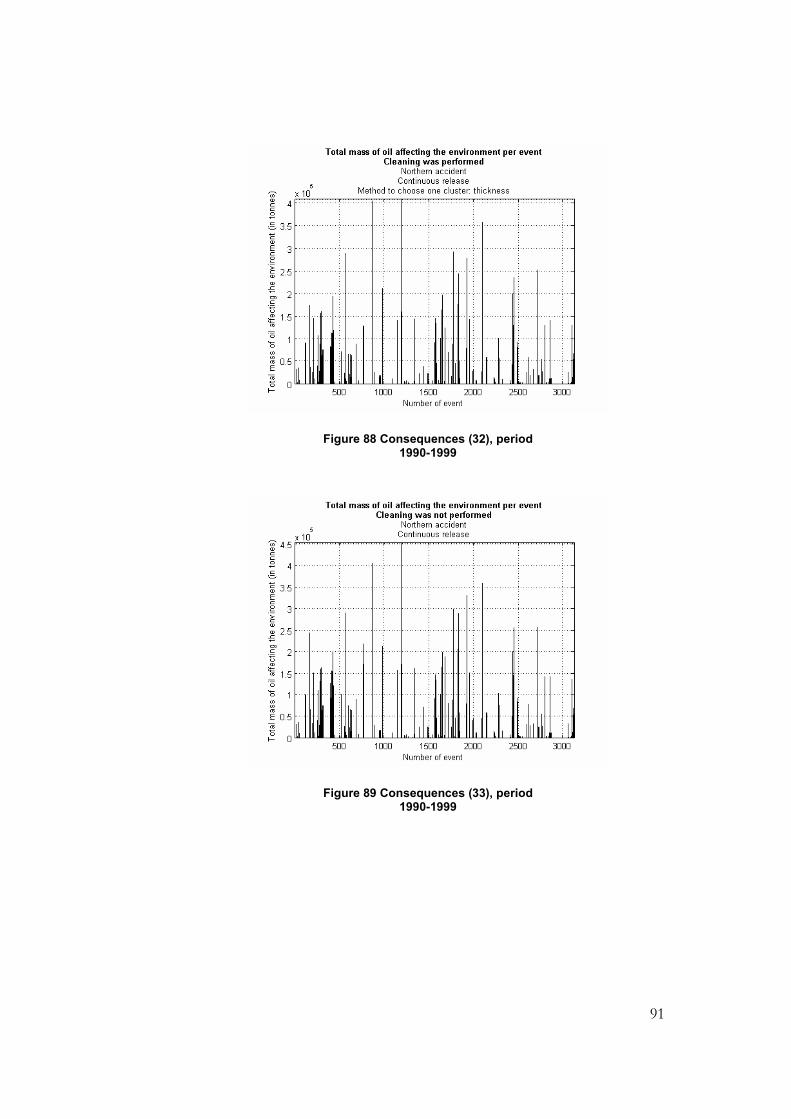
91
Figure 88 Consequences (32), period 1990-1999
Figure 89 Consequences (33), period 1990-1999

92
Figure 90 Consequences (34): most affected zone, period 1990-1999
Figure 91 Consequences (35), period 1990-1999

93
4.2.4 Northern accident. Method to choose one cluster: mass
The same conclusion that we reached when studying the results of
simulating southern accident can also be seen here. The cleaned
quantities are a little smaller when choosing a cluster based on
mass than when choosing it based on thickness. The following table
gives the some statistics for the quantity of oil removed.
Total quantity of oil removed
Mean 2260.581
Std 1676.003
Max 8553.635 1995 / 07 / 29 / 12
Min 0.000
19 events starting in one of the months:
01, 03, 09, 10, 11, 12
The next plot shows the mean quantity of oil cleaned in time. About
300 tonnes are removed on average in the first hour and the
quantity is decreasing, having one more increase at 7 hours when it
reaches a value of about 100 tonnes, while when using the
thickness-based method of choosing a cluster this increase reached
a value of 200 tonnes.

94
Figure 92 Cleaned oil in time (4), period 1990-1999
The consequences on the environment are presented bellow. The
values are almost identical to the ones presented in the previous
sub-section. We will therefore present just the mean total quantity of
oil affecting each zone when cleaning is performed.

95
Figure 93 Consequences (36), period 1990-1999

96
C h a p t e r 5
Analysis of the model
5.1 Comparisons between simulations’ results
Since the results presented in the previous chapter are many, and
many more could have been given, we will try to summarize them
here. The same types of results obtained simulating various
scenarios will be grouped and presented in tables. We will try to
analyze and explain them once more by pointing the similarities and
the differences.
The first table gives the mean total quantity of oil removed from the
water in the first 5 days after the accident in the specified scenarios.
Quantity of oil removed (averaged
on events) Southern accident Northern accident
Thickness 579 2738
Mass 471 2261
In the southern accident about 25% of the spilled quantity can be
removed in the first 5 days by mechanical cleaning. In a northern
accident only about 12% of the spilled quantity can be removed. We
have already concluded that this happens manly because different
types of oil are spilled in the two accidents. The oil spilled in the
southern accident is heavier and evaporates less than the one
spilled in a northern accident. The next table gives the mean total
quantity of oil evaporated in the two accidents.

97
Quantity of oil evaporated
(averaged on events) Southern accident Northern accident
Thickness / Mass 200 8074
In a southern accident 10% of the total amount of oil spilled
evaporates in the first 5 days, while in a northern accident 40%
evaporates. When the type of oil spilled evaporates faster, a smaller
amount remains to be cleaned. That makes the cleaning results
from the simulations of northern accidents be much worse than the
ones obtained from simulations of southern accidents.
We also concluded that from the two measures of choosing the
“best” cluster to be cleaned, the one based on thickness gives
better results. Intuitively this is a good result: looking for clusters
with a big thickness means looking for concentration of oil particles.
Eliminating the situation when a big and unreal value of thickness
appears for a cluster that has a very small area, but also a small
mass, choosing a thick cluster is in the same time choosing a big
mass and a small area. Compared to choosing just after mass, this
should give better results. If we are only interested in the mass of
the cluster, we can choose one cluster that has a big mass that is
however distributed on a very large area. This will make cleaning
that cluster less efficient than cleaning a lighter but covering a
smaller area cluster.
The next table shows the mean quantity of oil that is still at surface
after 5 days. This quantity is equal to the total quantity of spilled oil
minus the cleaned, evaporated and stranded quantities.

98
Quantity of oil still at surface (averaged on
events) Southern accident Northern accident
Thickness 695 7235
Mass 771 7642
In a southern accident about 35% of the quantity of spilled oil is still
at surface after 5 days. In a northern accident about 37% of the
spilled oil is still at surface after the first 5 days of mechanical
cleaning. Even if the cleaning measures are not that efficient, a
faster evaporation makes the percentage of oil left at surface in a
northern accident be almost equal with the one in a southern
accident.
The next table gives the total quantities of cleaned oil in the events
form the various scenarios when the maximum amount was
removed (maximum after all events considered).
Maximum quantity of oil removed
Southern accident Northern accident
Thickness 1625 8620
Mass 1618 8554
In a southern accident a maximum of over 80% of the total spilled
oil can be cleaned in the first 5 days, while in a northern accident a
maximum of 43% can be removed. The results from simulating
northern accidents are half worse, maintaining the pattern already
observed when talking about mean quantities.
The mean total quantities affecting the environment in the period of
5 days when mechanical cleaning is performed are given in the next
table.

99
Total quantity of oil affecting the environment
(averaged on events)
Southern accident Northern accident
Thickness 2151 5237
Mass 2286 5331
5.2 Results of simulating one event
In this section we will consider only one event and try to analyze it in
more detail. We will give plots and tables presenting values for all
variables significant in the cleaning module. We will also add some
plots that present the clusters at some specifics hours in the
simulation.
We will consider an event from the year 1995, namely 1995/06/14/
00.
It is a southern accident, a continuous release, and the cluster is
chosen at each hour in the simulation based on thickness. The
accident starts during the night, natural light being present after only
one hour (the twilight ends at 23:00 and begins again at 01:00). For
this reason, in the first hour only 50.740 tonnes are cleaned, and in
the second hour a bigger quantity of 83.970 tonnes is cleaned, the
multiple variable being 1 again.
The next table gives general results as the total quantities of oil
removed, evaporated and still at surface after 10 days.
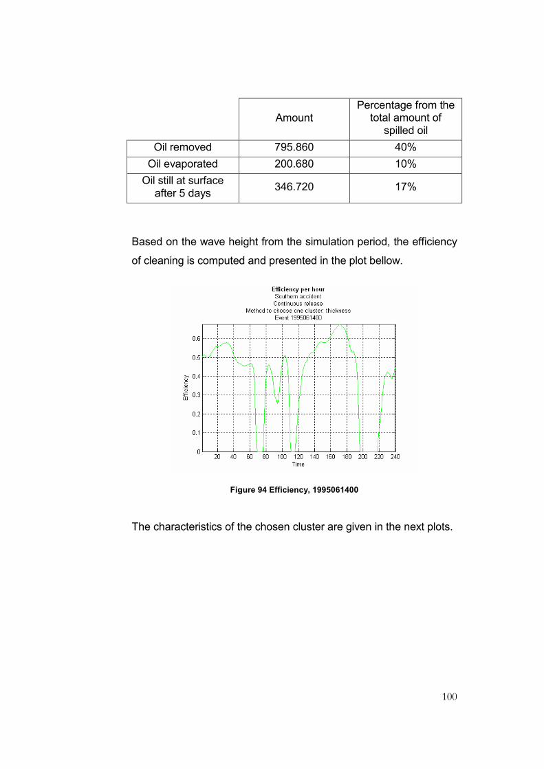
100
Amount Percentage from the
total amount of spilled oil
Oil removed 795.860 40%
Oil evaporated 200.680 10%
Oil still at surface after 5 days
346.720 17%
Based on the wave height from the simulation period, the efficiency
of cleaning is computed and presented in the plot bellow.
Figure 94 Efficiency, 1995061400
The characteristics of the chosen cluster are given in the next plots.

101
Figure 95 Mass of the chosen cluster, 1995061400
Figure 96 Area of the chosen cluster, 1995061400

102
Figure 97 Volume of the chosen cluster, 1995061400
Figure 98 Thickness of the chosen cluster, 1995061400

103
The quantity of oil removed in time is plotted bellow.
Figure 99 Cleaned oil, 1995061400
The most affected zone after this accident is zone number 7 with a
total amount of 5000 tonnes.

104
Figure 100 Consequences, 1995061400
The following two pictures show at two different moments in the
simulation the clusters formed from the oil particles that are at the
surface of water, the chosen cluster and the position of the cleaning
formation.
The first picture shows simulation components at 88 hours after the
moment of the first spill. In the right part we can see some statistics
like the quantity of oil cleaned in the current hour, the quantity of oil
cleaned up to this hour, the quantity of oil evaporated in the current
hour, the quantity of oil evaporated up to this hour, and the quantity
of oil at surface at the current hour. Also the time of the simulation
and the real time are given at the top and the wind speed and wave
height in the hour when the last cleaned cluster was chosen. In the
left part we can see a wind rose showing the direction of the wind.
The clusters formed are color coded according to their thickness

105
and the red line is showing the position of the cleaning vessels at
the end of this hour of cleaning.
Figure 101 Simulation snapshot t=88
The second picture gives the formed clusters at 208 hours after the
first spill.

106
Figure 102 Simulation snapshot t=209
5.3 Analysis of the clustering approach
An important question that comes to mind is whether or not the
approach we have chosen to deal with the mixture of particles is an
appropriate one. We will try to answer this question by simply
comparing the results of the model that uses clustering with the
results of a model that does not group the oil particles in any way.
The second model simply takes all particles at the surface of water
and considers them one big cluster. At each hour of the simulation
the cleaning vessels are assumed to be at the center of mass of the
big cloud of particles and they remove a quantity of oil (computed in
the same way as before) from the area that can be covered in that
hour.

107
We will use just the events from the year 1995 and simulate
continuous, southern accidents. The cleaning procedures are
performed for a period of 5 days and the amount of spilled oil is
represented by 500 particles.
The two plots bellow give the mean amount of oil hourly removed in
the two cases. The first plot is the result of the model when the
particles are grouped and one such group is chosen to be cleaned,
while the second plot is obtained with the model in which all
particles are considered as forming one big group.
Figure 103 Cleaned oil in time, year 1995, clustering
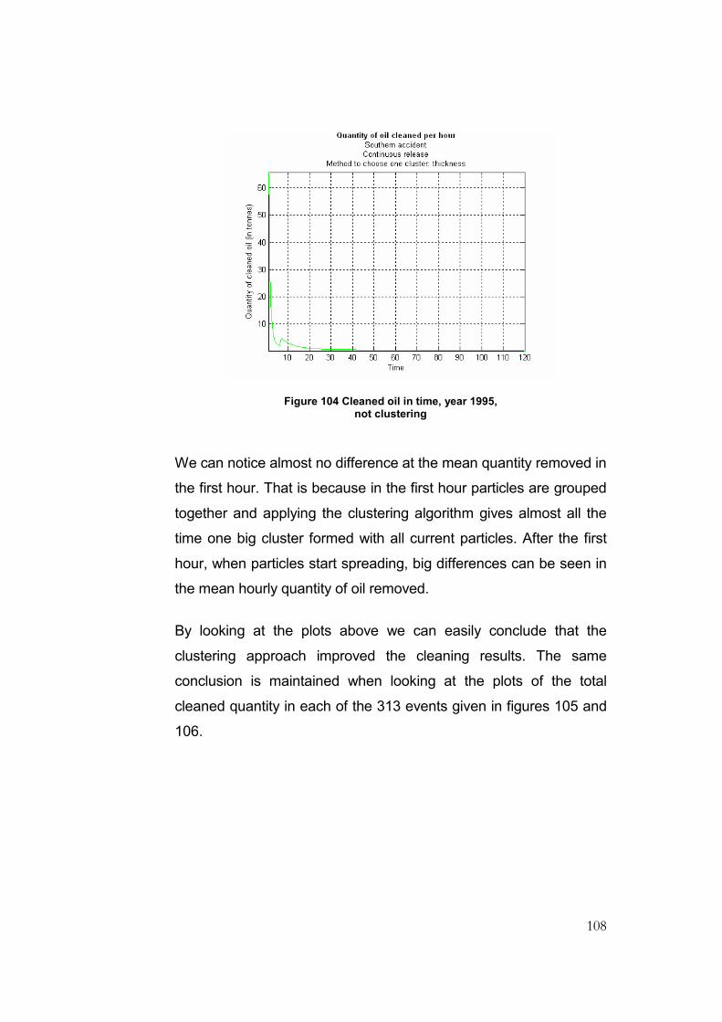
108
Figure 104 Cleaned oil in time, year 1995, not clustering
We can notice almost no difference at the mean quantity removed in
the first hour. That is because in the first hour particles are grouped
together and applying the clustering algorithm gives almost all the
time one big cluster formed with all current particles. After the first
hour, when particles start spreading, big differences can be seen in
the mean hourly quantity of oil removed.
By looking at the plots above we can easily conclude that the
clustering approach improved the cleaning results. The same
conclusion is maintained when looking at the plots of the total
cleaned quantity in each of the 313 events given in figures 105 and
106.

109
Figure 105 Cleaned oil per events, year 1995, clustering
Figure 106 Cleaned oil per events, year 1995, not clustering
Finally, we extract some numbers to stress the above conclusion.
The next table gives the mean, maximum, and minimum quantity of
oil removed in the two cases.

110
Clustering Not clustering
Mean quantity of oil removed
560 173
Maximum quantity of oil removed
1592 634
Minimum quantity of oil removed
0.015 0.010
5.4 Analysis of limiting factors for the cleaning performances
A very important task of this project is to find the limiting factors of
cleaning. By limiting factors we refer to those variables or
parameters that make the cleaning measures not to be 100%
efficient.
We have already proven in the previous section that the area of the
oil spill is a limiting factor. By showing that a clustering technique
improves the results of the model, we also showed that cleaning a
smaller area gives better results.
The parameters of the cleaning vessels could also limit the cleaning
results. However, they are either obtained from experts or assumed
by averaging values from real data. It is obvious that if the cleaning
speed of the vessels would be bigger, much more could be cleaned
since the area covered by the vessels in a given period of time
would be also bigger. The storage capacity could also be a limiting
factor, since the cleaning vessels can need to go to base to unload
if they are full and no tanker is available for immediate unload.

111
However, this was not the case in our simulations since the oil spills
that we considered were not too big.
The most important limiting factor we can think of is obviously the
weather. We will therefore try to find how big the influence of
weather on the cleaning results is. We account for the influence of
weather through two variables efficiency and allowance. We will
start by trying to find how big the influence of the wave height on the
cleaning results is. For this we will compare the results obtained
when the influence of waves was included through the variable that
gives the efficiency with the results obtained when considering that
the waves do not have any influence. That will mean that we simply
assume efficiency equal to 1 during the entire simulation. Again, we
consider all 313 events from the year 1995 and simulate southern,
continuous releases.
Of course, the weather is a limiting factor not by itself, but because
the technical limitations of the cleaning vessels. For wind speed or
wave height bigger than some threshold, the cleaning vessels can
not operate anymore. If this technical limitation would be overcome
or at least made smaller, the weather could be assumed to
influence less the efficiency of cleaning. Efficiency of cleaning could
be assumed to be 100% for example for wave height of 4 meters
instead of 2, and consequently bigger efficiency for the values
bellow 4 meters. However, as we already mentioned, the limits we
assumed for the wave height are given by experts. The results
obtained when efficiency is computed based on real wave data and
the above mentioned limits and when efficiency is assumed to be
100% on any wave conditions are presented in the next table.

112
Efficiency based on real wave data
Efficiency ≡ 1
Mean quantity of oil removed
560 1112
Maximum quantity of oil removed
1592 1781
Minimum quantity of oil removed
0.015 394
Differences can be seen in all three quantities; the most important is
at the mean quantities: when cleaning can not go on for wave
heights bigger than 2 meters a mean of 560 tonnes oil can be
removed, while when the cleaning can be performed for any wave
height this value doubles. The same can be noticed looking at the
plots that give the mean hourly quantity of oil removed in the two
cases (figures 107 and 108). We can observe that when the wave
height influences the efficiency of cleaning, in the first hour a mean
of 60 tonnes can be removed, while if the cleaning could be carried
on for any wave height, this value could be 140.
Figure 107 Cleaned oil in time, year 1995, efficiency based on real wave data
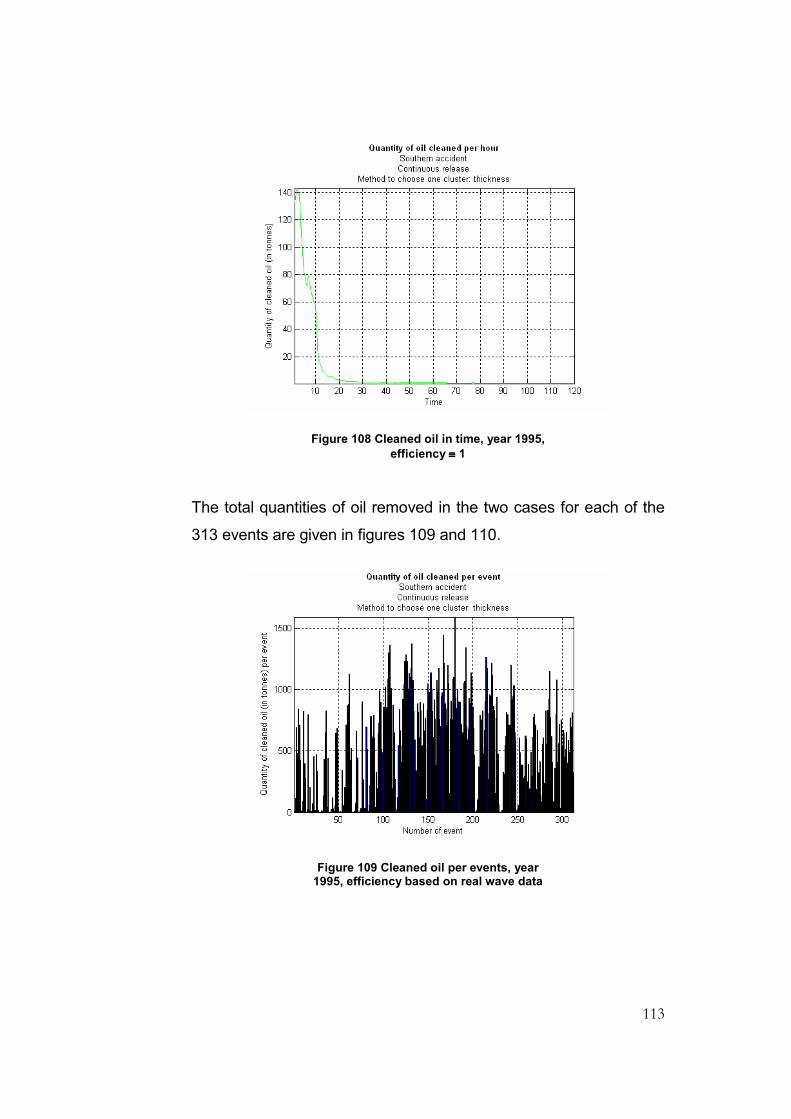
113
Figure 108 Cleaned oil in time, year 1995,
efficiency ≡≡≡≡ 1
The total quantities of oil removed in the two cases for each of the
313 events are given in figures 109 and 110.
Figure 109 Cleaned oil per events, year 1995, efficiency based on real wave data
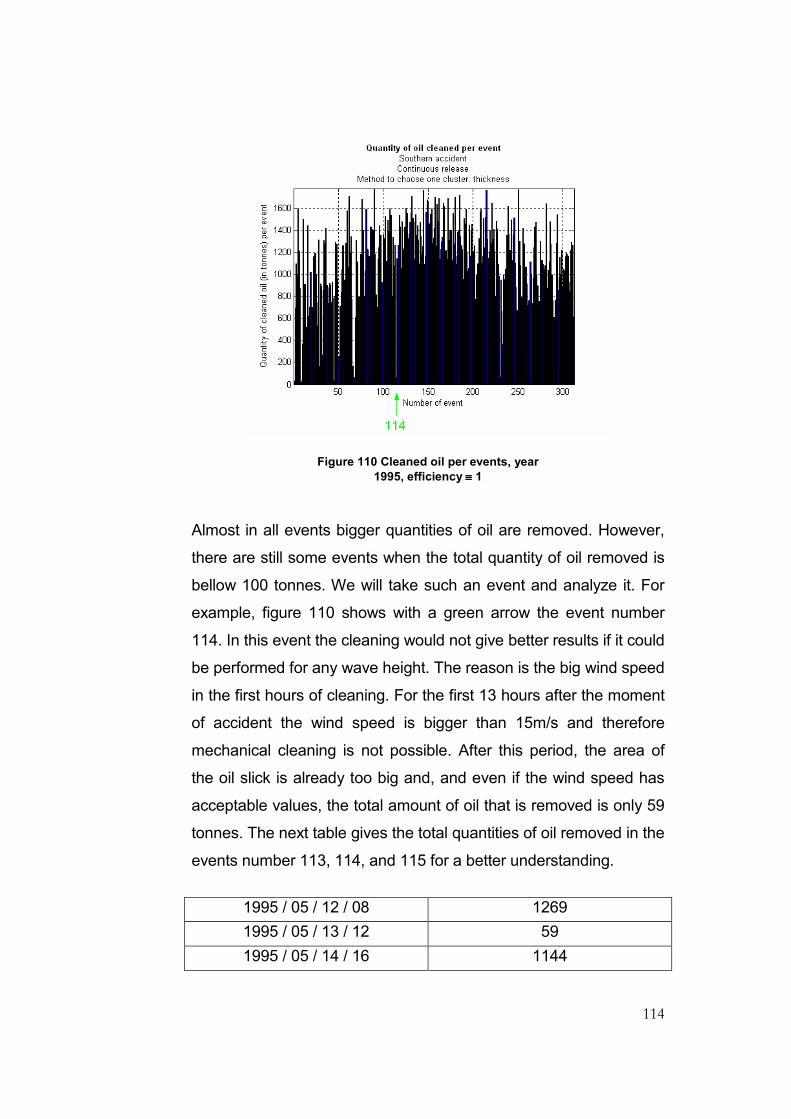
114
Figure 110 Cleaned oil per events, year
1995, efficiency ≡≡≡≡ 1
Almost in all events bigger quantities of oil are removed. However,
there are still some events when the total quantity of oil removed is
bellow 100 tonnes. We will take such an event and analyze it. For
example, figure 110 shows with a green arrow the event number
114. In this event the cleaning would not give better results if it could
be performed for any wave height. The reason is the big wind speed
in the first hours of cleaning. For the first 13 hours after the moment
of accident the wind speed is bigger than 15m/s and therefore
mechanical cleaning is not possible. After this period, the area of
the oil slick is already too big and, and even if the wind speed has
acceptable values, the total amount of oil that is removed is only 59
tonnes. The next table gives the total quantities of oil removed in the
events number 113, 114, and 115 for a better understanding.
1995 / 05 / 12 / 08 1269
1995 / 05 / 13 / 12 59
1995 / 05 / 14 / 16 1144

115
Since the events start at 28 hours intervals, the first 28 values of
wind speed from one event are identical with the hours 28-55 from
the event that preceded it. In the first event from the table above the
wind speed had acceptable values for the first 26 hours so cleaning
was performed. After this period, for 15 hours the wind speed had
bigger values than the acceptable limit. When the second event
started, at 28 hours after the start of the first event, the wind speed
was already too big and for the first 13 hours when the cleaning
could have been effective, no oil was removed. Again, after a
period, the wind speed values are again acceptable, so when the
third event starts, mechanical cleaning is possible.
From all above we can conclude that even if the wind and the
waves are correlated, there are some situations when the wind limit
for cleaning is exceeded, even if the waves have acceptable height.
We will therefore present the results obtained when assuming that
the cleaning can be carried on for both any values of wave height
and of wind speed. For comparison, the next table gives the values
for quantities of removed oil in all three cases.
Efficiency and allowance
based on real weather data
Efficiency ≡ 1
Allowance based on real wind data
Efficiency ≡ 1
Allowance ≡ 1
Mean quantity of oil removed
560 1112 1185
Maximum quantity of oil removed
1592 1781 1781
Minimum quantity of oil removed
0.015 394 402

116
Bellow, the plots of the mean hourly quantity of oil removed and the
total quantity of oil removed per events are given. We can note that
the differences are not that big compared to the corresponding ones
when the influence of waves was neglected, but are major
compared with the ones when both influences of wind and wave are
taken into account. The same conclusion can be drawn, of course,
from the table above.
Figure 111 Cleaned oil in time, year 1995,
efficiency ≡≡≡≡ 1, allowance ≡≡≡≡ 1
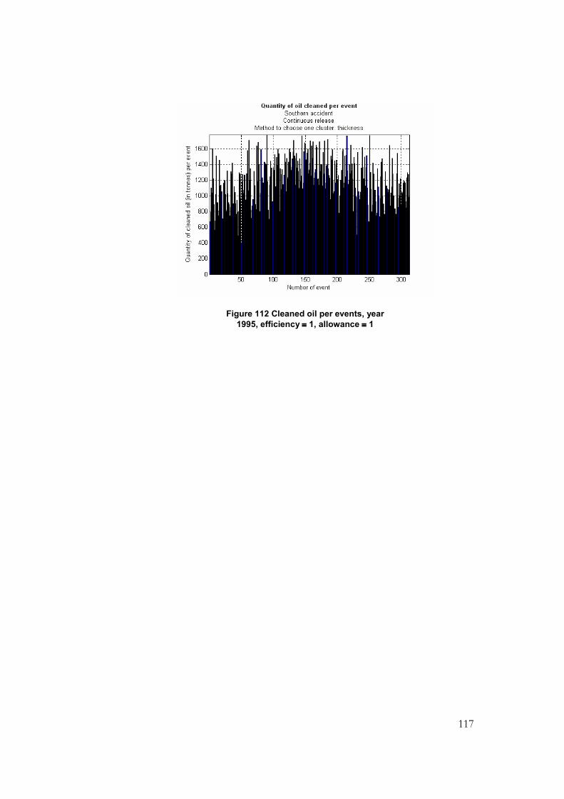
117
Figure 112 Cleaned oil per events, year
1995, efficiency ≡≡≡≡ 1, allowance ≡≡≡≡ 1
118
C h a p t e r 6
Conclusions and recommendations for further work
We developed a model for analyzing the consequences of an oil
spill that complements the oil-drift model by permitting to include
response measures. Two different types of accidents can be
simulated in which different quantities and types of oil are released.
We concluded that the type of oil that is spilled has a big influence
on the cleaning results. Also two kind of releases are implemented,
an instantaneous one and a continuous one. Comparing the results
from both types of releases we can observe that the instantaneous
release is an optimistic assumption, since in the first hour too much
oil can be removed from the water’s surface.
Two different strategies for cleaning are implemented: the cleaning
can be performed where the oil slick is thicker or where the mass of
oil is bigger. Comparing the results using these two different
strategies we conclude that choosing to clean where the oil slick is
thicker gives better results. This was an expected result, since it
seems more logical to aim to the thickest oil and not to the biggest
mass of oil that can be spread on a large area.
The damages on the German Wadden Sea coast were computed
and compared with the scenario when no cleaning measures are
taken.
We also tried to analyze the factors that limit the performances of
the cleaning. When oil is spilled at water it is crucial to contain it as
soon as possible because when the area of the oil slick becomes

119
larger, the quantities of oil that can be removed are very small.
Mechanical cleaning does not remove enough oil from the water
once the area covered by the slick is too big. We compared our
results with the results of a model that takes all current particles and
considers them one big cluster. Big differences were noticed,
showing the big impact of the area of the slick on the cleaning
results.
We can understand this easier giving some numbers. Considering a
vessel with wing span of 30m (that is exactly the total wing span of
the first formation of 5 vessels we consider in our model) and a
cleaning speed of 1kn, in one hour this vessel will cover an area of
only 0.056km2. In the same time, after only 20 hours the oil spilled in
a simulated southern accident covers an average area of 100km2
and after 5 days an average area of 800km2. Even the clusters
chosen to be cleaned have areas much bigger than what the vessel
can cover in one hour: a mean of 10km2 after about 20 hours and
more than 70km2 after 5 days. We can easily understand that the oil
slick is too widespread for the cleaning results to be satisfactory.
Very big differences were also observed when we compared our
results with the results of a model that assumes the cleaning could
be performed on any weather conditions.
As recommendations for future work, we can suggest considering
more positions for the accident. Like this the impact of the size, the
shape and the position of the wind parks can be analyzed. Also
different strategies for the cleaning operations can be implemented.
Maybe by monitoring the oil slick the cleaning can be conducted so
that to minimize the damages on some specific sensitivity area. The
clustering technique might also be improved. By analyzing the

120
various possible shapes of the oil slicks, maybe a specialized
clustering technique might seem more appropriate.

121
BIBLIOGRAPHY
Fingas, M, The basics of oil spill cleanup, Boca Raton, Lewis, 2001
Doerffer, J. W., Oil spill response in the maritime environment,
Oxford, Pergamon, 1992
Meyers, R. J., Oil spill response guide, Park Ridge, Noyes Data
Corporation, 1989
Tramier, B., A field guide to coastal oil spill control and clean-up
techniques, Den Haag, Concawe, 1981
Johnson, T. L., Oil spill cleanup: options for minimizing adverse
ecological impacts, Washington, American Petroleum Institute, 1985
Bijnen, E. J., Cluster Analysis, Tilburg University Press, 1973
Späth, H., Cluster Analysis Algorithms for Data Reduction and
Classification of Objects, Chichester, Horwood, 1980
Hartigan, J. A., Clustering Algorithms, New York, Wiley, 1985

I
APPENDIX 1
Classification of the oil types
Type of oil
Characteristics of oil Example
1
Light crude oil
Max. evaporation ca. 40%
Density ca. 850kg/m3
Crude No. 2
2
Heavy oil
Max. evaporation < 30%
Density 900kg/m3
Bunker C
3
Crude oil Africa, Near East
Max. evaporation 20-40%
Density ca. 850kg/m3
Crude Nigeria
4
Crude oil North Sea
Max. evaporation 30-50%
Density ca. 850kg/m3
Crude Statfjord
5
Crude oil
Max. evaporation > 50%
Density 800kg/m3
Crude Ekofisk
6
Light volatile petroleum products
Very high evaporation
Kerosene
7 Crude oil
Max. evaporation 20-50% Crude Venezuela
8 Very heavy oil
Low evaporation (<10%) IFO 450

II
APPENDIX 2
Example of twilight table
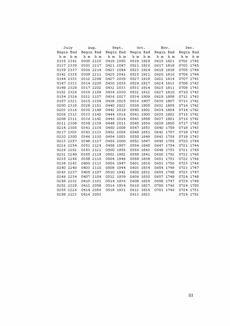
III
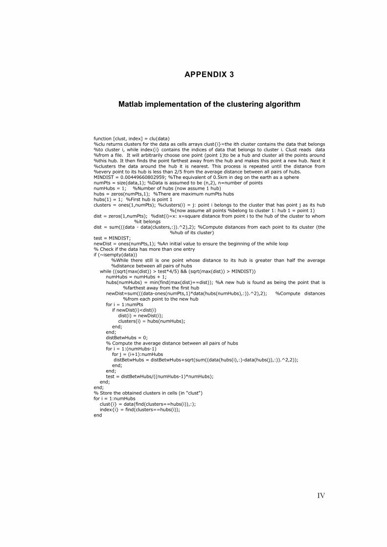
IV
APPENDIX 3
Matlab implementation of the clustering algorithm
function [clust, index] = clu(data)
%clu returns clusters for the data as cells arrays clust{i}=the ith cluster contains the data that belongs
%to cluster i, while index{i} contains the indices of data that belongs to cluster i. Clust reads data
%from a file. It will arbitrarily choose one point (point 1)to be a hub and cluster all the points around
%this hub. It then finds the point farthest away from the hub and makes this point a new hub. Next it
%clusters the data around the hub it is nearest. This process is repeated until the distance from %every point to its hub is less than 2/5 from the average distance between all pairs of hubs.
MINDIST = 0.00449660802959; %The equivalent of 0.5km in deg on the earth as a sphere
numPts = size(data,1); %Data is assumed to be (n,2), n=number of points
numHubs = 1; %Number of hubs (now assume 1 hub)
hubs = zeros(numPts,1); %There are maximum numPts hubs
hubs(1) = 1; %First hub is point 1
clusters = ones(1,numPts); %clusters(i) = j: point i belongs to the cluster that has point j as its hub
%(now assume all points %belong to cluster 1: hub 1 = point 1)
dist = zeros(1,numPts); %dist(i)=x: x=square distance from point i to the hub of the cluster to whom
%it belongs dist = sum(((data - data(clusters,:)).^2),2); %Compute distances from each point to its cluster (the
%hub of its cluster)
test = MINDIST;
newDist = ones(numPts,1); %An initial value to ensure the beginning of the while loop
% Check if the data has more than one entry
if (~isempty(data))
%While there still is one point whose distance to its hub is greater than half the average
%distance between all pairs of hubs
while ((sqrt(max(dist)) > test*4/5) && (sqrt(max(dist)) > MINDIST)) numHubs = numHubs + 1;
hubs(numHubs) = min(find(max(dist)==dist)); %A new hub is found as being the point that is
%farthest away from the first hub
newDist=sum(((data-ones(numPts,1)*data(hubs(numHubs),:)).^2),2); %Compute distances
%from each point to the new hub
for i = 1:numPts
if newDist(i)<dist(i)
dist(i) = newDist(i);
clusters(i) = hubs(numHubs);
end; end;
distBetwHubs = 0;
% Compute the average distance between all pairs of hubs
for i = 1:(numHubs-1)
for j = (i+1):numHubs
distBetwHubs = distBetwHubs+sqrt(sum((data(hubs(i),:)-data(hubs(j),:)).^2,2));
end;
end;
test = distBetwHubs/((numHubs-1)*numHubs); end;
end;
% Store the obtained clusters in cells (in "clust")
for i = 1:numHubs
clust{i} = data(find(clusters==hubs(i)),:);
index{i} = find(clusters==hubs(i));
end

V
APPENDIX 4
Some Matlab functions and scripts
The first two scripts give the parameters of the model. 1. parameters
% South accident
oilDensity = 0.9*10^12; %in kg/km^3 (Bunker C)
% % North accident
%oilDensity = 0.85*10^12; %in kg/km^3 (Crude Nigeria)
% Port's coordinates
portLongitude = 8.70; portLatitude = 53.866;
portLocation = [portLongitude portLatitude];
% Loading base's coordinates
baseLongitude = 8.50;
baseLatitude = 53.90;
baseLocation = [baseLongitude baseLatitude];
% Prepositioned vessels's characteristics
numPPV = 5; % Number of prepositioned vessels;
%storCapPPV = 15*10^-7; % in km^3 Storage capacity of one vessel (1500 m^3) storCapPPV = 15*10^-7; % in km^3 Storage capacity of one vessel (1500 m^3)
wingSpanPPV = 0.006; % in km Wing Span of one vessel
ppvTSpeed = 15; % Travelling speed in knots
ppvTSpeed = ppvTSpeed*1.8523; % Travelling speed in km/h
ppvCSpeed = 1; % Cleaning speed in konts
ppvCSpeed = ppvCSpeed*1.8523; % Cleaning speed in km/h
totalPPVCapacity = numPPV*storCapPPV*oilDensity; % Formation's storage capacity in kg
totalPPVSpan = numPPV*wingSpanPPV; % Formation's wing span in km
% From port vessels's characteristics numPV = 5; % Number of vessels from port;
storCapPV = 5*10^-7; % Storage capacity of one vessel in km^3 (500 m^3)
wingSpanPV = 0.01; % Wing Span of one vessel in km
pvTSpeed = 15; % Travelling speed in knots
pvTSpeed = pvTSpeed*1.8523; % Travelling speed in km/h
pvCSpeed = 1; % Cleaning speed in konts
pvCSpeed = pvCSpeed*1.8523; % Cleaning speed in km/h
totalPVCapacity = numPV*storCapPV*oilDensity; % Formation's storage capacity in kg
totalPVSpan = numPV*wingSpanPV; % Formation's wing span in km
% Capacity and wing span of both formations totalCapacity = totalPPVCapacity + totalPVCapacity;
totalSpan = totalPPVSpan + totalPVSpan;
% Cleaning Rate
ppvCleaningRate = 300*10^3; % in kg
pvCleaningRate = 500*10^3; % in kg
cleaningRate = [numPPV*ppvCleaningRate numPV*pvCleaningRate
numPPV*ppvCleaningRate+numPV*pvCleaningRate];
2. globalParameters
% Declare global variables global ageParticlesInCluster allParticles baseLocation cg cleaned cleanedPerHour cleanerLocation …
cleanerHere cleaningRate clust clusterArea clusterLocation clusterMass clusterMassOverArea …
clusterThickness clusterVolume clusterToClean currentParticles dayOfSpill dispersed evap index …
indexClusterToClean inPortOrOnWay isPossibleToClean hourOfSpill lastBase …
locationNewCenterOfGravity locationPPV locationSpill massParticlesInCluster maxTime …

VI
monthOfSpill numParticles oilDensity oilAtSurfacePerHour oilMass onPlace quantityCleaned …
quantityCleanedNow ppvCSpeed ppvTSpeed PPVPV timeToCluster timeToGoToCluster …
timeToReturn toKeep totalCapacity totalPPVCapacity totalPVCapacity totalPPVSpan totalPVSpan …
stranded totalSpan waterContent waveHeight windComponents windSpeed
global StartingDateTime EndingDateTime EventTimeInterval
StartingDateTime = [1995 01 01 16];
EndingDateTime = [1995 12 31 16];
% StartingDateTime = [1990 01 01 20];
% EndingDateTime = [1999 12 26 16];
% StartingDateTime = [1990 01 01 20];
% EndingDateTime = [1995 03 22 00];
EventTimeInterval = 28;
global timeStep
timeStep = 1; % in hours; global eventId eventIndex
global subdir1 subdir2
% For contiuous release
subdir1 = 'Continuous';
% For not contiuous release
%subdir1 = 'Not_continuous';
%subdir2 = '1995/';
subdir2 = '1990-1999/';
% Type of accident subdir3 = 'South';
% subdir3 = 'North';
global chooseClusterMethod
chooseClusterMethod = 'clusterThickness';
%chooseClusterMethod = 'clusterMass';
global table
global isNight
global earthEllipsoid
if(isempty(earthEllipsoid))
earthEllipsoid = almanac('earth','ellipsoid','kilometers'); end
global massC thicknessC areaC eff timeToCleanC volumeC
global z massZ
The next function reads data from 4 files given as parameters.
3. readData
function readData(file1, file2, file3, file4);
% Modified variables: allParticles, evap, locationSpill, numParticles, maxTime, totalQuantOil,
%waterContent, waveHeight, windComponents
% numParticles = number of particles considered for the total release
% maxTime = maximum time of following the particles
% allParticles = cell array with information for all particles
% evap = vector that contains the percentage that evaporates in each hour for h = 0:maxTime, %where evap(0) = 0 and evap(1) = percentage that evaporates in the first hour after the accident
% waterContent = vector that contains the percentage of water in the oil slick of each hour
% Define global variables
globalParameters;
%%%%%%%%%%%%%%%
% READ FILE 1 %
%%%%%%%%%%%%%%%
% Read data for event_x (file1) and get the information for particles; get the percentage of
%evaporation and the water content from oil_infos_y (file2)
% Open the data file for reading only fid = fopen(file1);
% Read number of particles (trajectories)
numParticles = fscanf(fid, 'Number of trajectories: %d\n');
% Read maximum time of following the particles
maxTime = fscanf(fid,'Maximum time steps stored: %d\n');
% Read total quantity of oil spilled (in tonnes)
totalQuantOil = fscanf(fid, '%d', 1);
% Initial mass of oil per particle (in kg)
initMass = totalQuantOil*10^3/numParticles; % Read longitude of the oil spill
% For continuous release (10 releases)

VII
% Check the type of oil == north <-> south
% SOUTH
aux1_1 = fscanf(fid,'t Bunker C (10 hours continuous release)\n Location of Oil Spill: %d');
% NORTH
%aux1_1 = fscanf(fid,'t Crude Nigeria (10 hours continuous release)\n Location of Oil Spill: %d');
% For non-continuous release
% Check the type of oil == north <-> south
%SOUTH
%aux1_1 = fscanf(fid,'t Bunker C\n Location of Oil Spill: %d');
% NORTH
%aux1_1 = fscanf(fid,'t Crude Nigeria\n Location of Oil Spill: %d');
aux1_2 = fscanf(fid, ':%d', 1);
aux1_3 = fscanf(fid, ':%d', 1);
longSpill = aux1_1 + aux1_2/60 + aux1_3/3600; % Read latitude of the oil spill
aux2_1 = fscanf(fid,' / %d', 1);
aux2_2 = fscanf(fid, ':%d', 1);
aux2_3 = fscanf(fid, ':%d\n', 1);
latSpill = aux2_1 + aux2_2/60 + aux2_3/3600;
locationSpill = [longSpill, latSpill];
% Read the extra text (26 lines)
fgets(fid); fgets(fid); fgets(fid); fgets(fid); fgets(fid);
fgets(fid); fgets(fid); fgets(fid); fgets(fid); fgets(fid); fgets(fid); fgets(fid); fgets(fid); fgets(fid); fgets(fid);
fgets(fid); fgets(fid); fgets(fid); fgets(fid); fgets(fid);
fgets(fid); fgets(fid); fgets(fid); fgets(fid); fgets(fid); fgets(fid);
% Read time of beginning and ending the simulation
% fscanf(fid,' Time at Oil Spill: 1998_11_07 (01:00) End of Simulation: 1998_11_17 (01:00)\n');
fscanf(fid,' Time at Oil Spill: ');
yearOfSpill = fscanf(fid, '%4c', 1);
fscanf(fid,'_');
monthOfSpill = fscanf(fid, '%2c', 1);
fscanf(fid,'_'); dayOfSpill = fscanf(fid, '%2c', 1);
fscanf(fid,' (');
hourOfSpill = fscanf(fid, '%2c', 1);
timeOfSpill = strcat(yearOfSpill, monthOfSpill, dayOfSpill, hourOfSpill, '0000');
fscanf(fid, ':00) End of Simulation: ');
yearOfEnding = fscanf(fid, '%4c', 1);
fscanf(fid,'_');
monthOfEnding = fscanf(fid, '%2c', 1);
fscanf(fid,'_'); dayOfEnding = fscanf(fid, '%2c', 1);
fscanf(fid,' (');
hourOfEnding = fscanf(fid, '%2c', 1);
timeOfEnding = strcat(yearOfEnding, monthOfEnding, dayOfEnding, hourOfEnding, '0000');
fscanf(fid, ':00)\n');
% Read the extra line
fgets(fid);
% Start reading the data for particles
for i = 1:numParticles
fscanf(fid,'%d', 1); % Read the "life" for each particle (the number of hours before going
% to the bottom of sea or on land
life(i) = fscanf(fid, '%d', 1);
% Read the time of "birth" for each particle (0 = it was produced in
% the first release, 7 = it was produced in the last release
fscanf(fid, '%d\n', 2);
% Read the coordinates for each particle
allParticles{i} = fscanf(fid, '%d %f %f %f %f %d\n', [6, (life(i)+1)])';
% Each particle attributes (coordinates, born, initial mass) are stored % in a cell
allParticles{i} = [allParticles{i}(:,[2:3]) initMass*ones(life(i)+1, 1) allParticles{i}(:,[4,6])];
end;
fclose(fid);
%%%%%%%%%%%%%%%
% READ FILE 2 %
%%%%%%%%%%%%%%%
% Read oil info's from oil_infos_1998110701
% Open the data file for reading only
% Read the extra text (34 lines) fid = fopen(file2);

VIII
fgets(fid); fgets(fid); fgets(fid); fgets(fid); fgets(fid);
fgets(fid); fgets(fid); fgets(fid); fgets(fid); fgets(fid);
fgets(fid); fgets(fid); fgets(fid); fgets(fid); fgets(fid);
fgets(fid); fgets(fid); fgets(fid); fgets(fid); fgets(fid);
fgets(fid); fgets(fid); fgets(fid); fgets(fid); fgets(fid); fgets(fid); fgets(fid); fgets(fid); fgets(fid); fgets(fid);
fgets(fid); fgets(fid); fgets(fid); fgets(fid);
% Read the data and put it in a matrix
e = fscanf(fid, ' %f %f %f %f %f %f', [6, inf])';
% Get the quantity spilled (per hour)
q = e(:, 1);
% Get the evaporated quantity
% Get the cummulative percentage of evaporation (per hour)
cumEvap = e(:, 2)/100;
% Get the cumulative quantity evaporated per hour cumQE = q.*cumEvap;
% Get the quantity evaporated in each hour
evap = cumQE - [0; cumQE(1:end-1)]; % in tones
% Get this quantity in kg
evap = evap*1000; % in kg
evap = evap(2:end); % maxTime hours = components
% Get the dispersed quantity in each hour
dispersed = q.*(e(:, 5)/100);
dispersed = dispersed*1000; % in kg dispersed = dispersed(2:end);
% Get the stranded quantity in each hour
stranded = q.*(e(:, 3)/100);
stranded = stranded - [0; stranded(1:end-1)];
stranded = stranded*1000; % in kg
stranded = stranded(2:end);
% Get the content in water (per hour)
% Get the percentage of water (per hour)
% In one unity of volume waterContent from the volume is water, the rest
% is oil waterContent = e(:, 6)/100;
fclose(fid);
%%%%%%%%%%%%%%%%%%%%%
% Read wave heights %
%%%%%%%%%%%%%%%%%%%%%
% Open the file for reading only
fid = fopen(file3);
w = fscanf(fid, '%lg %f %f', [3, inf])';
% Get the wave heights for the event considered index = find((w(:,1) >= str2num(timeOfSpill)) & (w(:,1)<= str2num(timeOfEnding)));
waveHeight = w(index, 2);
fclose(fid);
%%%%%%%%%%%%%%%%%%%%%%%%
% Read wind components %
%%%%%%%%%%%%%%%%%%%%%%%%
% Open the file for reading only
fid = fopen(file4);
fgets(fid);
fgets(fid); ww = fscanf(fid, '%lg %f %f', [3, inf])';
% Get the windcoordinates for the event considered
% Put the time in the right format for comparison
date1 = strcat(yearOfSpill, monthOfSpill, dayOfSpill, hourOfSpill);
date2 = strcat(yearOfEnding, monthOfEnding, dayOfEnding, hourOfEnding);
index = find((ww(:,1) >= str2num(date1)) & (ww(:,1)<= str2num(date2)));
windComponents = ww(index, 2:3);
fclose(fid);
The next 2 scripts account for the influence of weather on the cleaning.

IX
4. efficiency
function eff = efficiency(wave);
% Computes the efficiency of cleaning (function of the wave height): takes value 1 if the wave %height is 0, 0 if the wave height is 2, and linearly decreases with the wave height if the wave
%height is between 0 and 2
%eff = 1;
% eff = -0.4*wave*(wave>=0&wave<=0.25) -0.8*wave*(wave>0.25&wave<=0.5) - ..
0.4*wave*(wave>0.5&wave<=0.75) - 0.2667*wave*(wave>0.75&wave<=1.5) - …
0.8*wave*(wave>1.5&wave<=2) + 1*(wave>=0&wave<=0.25) + … 1.1*(wave>0.25&wave<=0.5)
+ 0.9*(wave>0.5&wave<=0.75) + … 0.8*(wave>0.75&wave<=1.5) + 1.6*(wave>1.5&wave<=2) +
0*(wave>2);
5. allowance
function allow = allowance(wind);
% Computes an allowance variable that takes value 1 if the wind speed is
% less than 15m/s (the mechanical cleaning is possible), and 0 otherwise
if wind <= 15
allow = 1;
else
allow = 0;
end; %allow = 1;
The next function computes characteristics of the clusters, like area, mass, volume and thickness.
6. clusterPropreties
function clusterProperties(t)
% Modified variables: ageParticlesInCluster, cg, clusterArea, clusterMass, clusterMassOverArea,
% clusterThickness , clusterVolume, isPossible, massParticlesInCluster, toKeep
% clust{i} contains the coordinates of the points that belong to the ith cluster, index{i} contains the
%indices in the coordCurrentParticles of the points that belong to the ith cluster
% The function computes properties for clusters (total mass, age of particles inside, area, thickness,
%etc.) to use for the selection of the cluster to clean
% These properties are computed only for clusters with more than 3 points and the indices of those %clusters in the array of all clusters is given by toKeep
% Define the global variables
globalParameters;
% Init the output of the function
isPossibleToClean = 1; % Variable that takes 1 if there are clusters with more than 3 points, 0
%otherwise
clusterThickness = []; % Vector containing thickness values for the clusters with more than 3 points
clusterMassOverArea = []; % Vector containing mass/area values for the clusters with more than 3
%points
cg = []; % Matrix containing on each line centers of gravity for the clusters with more than 3 points toKeep = []; % Vector containing the indices of the clusters kept (that have more than 3 points)
clusterMass = [];
clusterArea = [];
clusterVolume = [];
ageParticlesInCluster = [];
massParticlesInCluster = [];
% Test for clusters with less than 3 particles
numClusters = size(clust,2); % number of clusters found
% Test if a cluster has less than 3 points toNeglect = []; % Indices of clusters that have less than 3 points
for k = 1:numClusters
if size(clust{k},1) < 3 % Number of points in a cluster
toNeglect = [toNeglect k];
end;
end;
toKeep = setdiff((1:numClusters),toNeglect);

X
if ~isempty(toKeep)
clust = {clust{toKeep}}; % Keep for the analysis only the clusters with more than 2 points
index = {index{toKeep}}; % Keep for the analysis only the clusters with more than 2 points
else
clust = {allParticles{currentParticles{t}}}; for i = 1:length(clust)
auxclus(i,:) = clust{i}(t,1:2);
end;
clust = {auxclus};
index = {(1:length(currentParticles{t}))};
end;
% Test for clusters with area 0
areaZero = [];
if isPossibleToClean == 1
numClusters = size(clust,2); % number of clusters kept for the analysis clusterConvHull = cell(numClusters, 1);
for k = 1:numClusters % Compute propreties for each cluster
% Get the convex hull of each cluster (contains the indices - in the original data - of the points
%that make the convex hull; get the first point twice)
%clusterConvHull{k} = convhull(clus{k}(:,1), clus{k}(:,2));
[clusterConvHull{k}, clust{k}] = convexhull2D(clust{k}, 4);
clusterConvHull{k} = clusterConvHull{k}(1:end-1);
% Compute the area of each cluster LAT LONG
clusterArea(k) = areaint(clust{k}(clusterConvHull{k},2), clust{k}(clusterConvHull{k},1), earthEllipsoid);
% Check if the area is zero (collinear points)
if clusterArea(k) == 0
areaZero = [areaZero k];
end;
end;
end;
% Take out of the analysis also the clusters with area = 0
toKeep = setdiff((1:numClusters), areaZero);
clust = {clust{toKeep}}; % Keep for the analysis only the clusters with area bigger than 0 index = {index{toKeep}}; % Keep for the analysis only the clusters with area bigger than 0
clusterArea = clusterArea(toKeep); % Keep the area only for the clusters with area bigger than 0
clusterConvHull = {clusterConvHull{toKeep}};
% Start again computing properties for the remaining clusters
% Is there any cluster left?
if(isempty(clust))
isPossibleToClean = 0;
end;
if isPossibleToClean == 1 numClusters = size(clust,2); % number of clusters kept for the analysis
clusterMass = zeros(numClusters,1); % Contains the mass for all clusters
massParticlesInConvHull = cell(numClusters, 1);
for k = 1:numClusters % Compute properties for each cluster
% Get the convex hull of each cluster (contains the indices - in the original data – of the points
%that make the convex hull; get the first point twice)
%clusterConvHull{k} = convhull(clus{k}(:,1), clus{k}(:,2));
%clusterConvHull{k} = convexhull2D(clus{k}');
%clusterConvHull{k} = clusterConvHull{k}(1:end-1);
% Compute the area of each cluster LAT LONG %clusterArea(k) = areaint(clus{k}(clusterConvHull{k},2), clus{k}(clusterConvHull{k},1),
earthEllipsoid);
ageParticlesInCluster{k} = [];
massParticlesInCluster{k} = [];
sizeCluster = size(clust{k},1);
for j = 1:sizeCluster
particleNum = currentParticles{t}(index{k}(j));
clusterMass(k) = clusterMass(k) + allParticles{particleNum}(t,3);
massParticlesInCluster{k} = [massParticlesInCluster{k} allParticles{particleNum}(t,3)]; ageParticlesInCluster{k} = [ageParticlesInCluster{k} (1-floor((particleNum-1)/100))];
end;
% Get the center of gravity of the convex hull of the cluster
massParticlesInConvHull{k} = massParticlesInCluster{k}(clusterConvHull{k});
cg(k,:) = centerGravity([clust{k}(clusterConvHull{k},1), clust{k}(clusterConvHull{k},2)],
massParticlesInConvHull{k});
% waterContent is recorded hourly and with regard to total number
% of particles; the water content per cluster is needed to
% compute the cluster's volume
% volume = volume(oil)+volume(water) clusterVolume(k) = (clusterMass(k)/oilDensity)/(1-waterContent(t+1));

XI
% clusterThickness(k) = (clusterVolume(k)/clusterArea(k))*10^5; % in centimeters
if ((clusterArea(k)<10^-6) && (sizeCluster<0.1*length(currentParticles{t})))
clusterThickness(k) = 0;
else
clusterThickness(k) = (clusterVolume(k)/clusterArea(k))*10^5; % in centimeters end;
% clusterMassOverArea(k) = clusterMass(k)/clusterArea(k);
end;
end;
toKeep = (1:size(clust,2));
The next function is used to choose one cluster from all clusters to be cleaned based on two possible strategies: the method to choose one cluster, methodToChooseCluster, can be clusterThickness or clusterMass.
7. clusterPropreties
function chooseCluster(method) % Modified variables: indexClusterToClean, clusterToClean, timeToGoToCluster
% Select the cluster to clean, knowing the clusters from which to choose and some characteristics
% Define the global variables
globalParameters;
% Choose a cluster if a cleaner is present
if(cleanerHere(1))
if(isPossibleToClean)
% Compute distances from clusters to cleaning boat (in km)
clusterCleanBoatDistance = distance(cg(:,2), cg(:,1), cleanerLocation(1,2)*ones(size(cg,1),1), cleanerLocation(1,1)*ones(size(cg,1),1), earthEllipsoid)';
% Compute time to reach the clusters (in hours)
clusterCleanBoatTime = clusterCleanBoatDistance/ppvTSpeed;
% % That's just to check if the time is so important
% clusterCleanBoatTime = ones(1,length(clusterCleanBoatTime))*1e-10;
% Check if the time is less than 1 hour
inTime = find(clusterCleanBoatTime < timeStep);
% Try if there are clusters
isPossibleToClean = ~isempty(inTime);
if(~isPossibleToClean) inTime = (1:size(cg,1));
clusterCleanBoatTime(inTime) = 1;
end
else
disp('No cluster around!!!(');
end
else % If no cleaner present we will consider all clusters to get the cluster location
if(isPossibleToClean)
inTime = (1:size(cg,1)); clusterCleanBoatTime(inTime) = 1;
else
disp('No cluster around!!!(');
end
end
if(isPossibleToClean)
% Choose even if we will never reach the cluster
%However, in this case isPossibleToClean will be 0
switch method % Choose the cluster with the biggest thickness
case {'clusterThickness'}
measure1 = (clusterThickness(inTime)).*(1 - clusterCleanBoatTime(inTime));
ind = find(max(measure1) == measure1);
ind = ind(1);
% Choose the cluster with the biggest mass
case {'clusterMass'}
measure2 = (clusterMass(inTime))'.*(1 - clusterCleanBoatTime(inTime));
ind = find(max(measure2) == measure2);
ind = ind(1); end
indexClusterToClean = toKeep(inTime(ind)); % Index in original clust

XII
clusterToClean = clust{indexClusterToClean};
timeToGoToCluster = clusterCleanBoatTime(inTime(ind));
clusterLocation = cg(inTime(ind),:);
else
disp('No cluster around!!!('); end
Having all properties of the chosen cluster, the next function is used to simulate the cleaning operations.
8. clean
function clean(t);
%This function computes how much can be cleaned, organizes the cleaning operation (which vessels
%clean and what is really cleaned = quantityCleanedNow), and does the cleaning
% Define global variables
globalParameters;
% Assume that at the end of this hour nothing changes
cleanerHere(2) = cleanerHere(1);
isNight(2) = isNight(1); PPVPV(2) = PPVPV(1);
inPortOrOnWay(2,:) = inPortOrOnWay(1,:);
cleanerLocation(2,:) = cleanerLocation(1,:);
% Cleaner's speed is the same no matter what vessels are used
cleanerSpeed = ppvCSpeed;
% Compute the time needed by the cleaner to reach the cluster from the base (needed to check if the
%cleaner can return from the base)
% If a cleaner is already there, the other needs to go to the same position (cleanerLocation), otherwise
%it needs to go to the clusterLocation
if(cleanerHere(1)) timeFromBase = distance([lastBase(1,2);lastBase(1,4);lastBase(1,6)],...
[lastBase(1,1);lastBase(1,3);lastBase(1,5)],...
cleanerLocation(1,2)*ones(3,1),...
cleanerLocation(1,1)*ones(3,1), earthEllipsoid)'/ppvTSpeed;
else
timeFromBase = distance([lastBase(1,2);lastBase(1,4);lastBase(1,6)],...
[lastBase(1,1);lastBase(1,3);lastBase(1,5)],...
clusterLocation(1,2)*ones(3,1),...
clusterLocation(1,1)*ones(3,1), earthEllipsoid)'/ppvTSpeed; end;
% Multiplication factor for the efficiency with respect to day/night
% When day: full efficiency, when night: half efficiency
if ~isNight(1)
multiplic = 1;
else
multiplic = 0.5;
end;
if(cleanerHere(1) && (length(currentParticles{t})>2) && isPossibleToClean)
% Get what is needed to compute the quantity that can be cleaned % First get the mass of particles in the cluster chosen for cleaning
% Get the particles inside the cluster
partic = currentParticles{t}(index{indexClusterToClean});
newMassParticlesInCluster = [];
for i = 1:size(partic)
newMassParticlesInCluster = [newMassParticlesInCluster allParticles{partic(i)}(t + 1, 3)];
end;
masses = newMassParticlesInCluster;
indexInToKeep = find(toKeep == indexClusterToClean);
% Get the mass, area and center of gravity and volume of the cluster
mass = clusterMass(indexInToKeep); % in kg
area = clusterArea(indexInToKeep); % in km2
center = cg(indexInToKeep,:);
volume = clusterVolume(indexInToKeep); % in km3
thickness = clusterThickness(indexInToKeep);% in cm
% Store some attributes for checks
massC(t) = mass;
areaC(t) = area;
XIII
volumeC(t) = volume;
thicknessC(t) = thickness;
timeToCleanC(t) = 1 - timeToGoToCluster;
% toClean depends on the vessels that are used for cleaning: toClean(1)=what can be cleaned
%only with PPV, toClean(2)=what can be cleaned only with PV, and toClean(3)=what can be %cleaned with both PPVPV
cleanerSpan = [totalPPVSpan, totalPVSpan, totalSpan]; %in Km
% Other parameters
eff(t) = efficiency(waveHeight(t));
allow = allowance(windSpeed(t));
areaCovered = cleanerSpeed*cleanerSpan*(1-timeToGoToCluster);
areaCovered(areaCovered > area) = area;
% Compute toClean using only the cluster's thickness and compare the obtained value with an
%upper limit of 440t per hour
able = (areaCovered*mass*(thickness*10^-5)*allow)/volume; % in kg for i = 1:3
if able(i) < cleaningRate(i)
toClean(i) = able(i)*eff(t)*multiplic;
else
toClean(i) = cleaningRate(i)*eff(t)*multiplic;
end;
end
end
% Init the quantity cleaned now quantityCleanedNow = 0;
% Test if the tanker has arrived (if so, capacity is unlimited)
if t < 25 % if1 % The tanker is was not here
if PPVPV(1) == 1 % ppv and pv were together % if2
if ~inPortOrOnWay(1,3) % if3 % They were here
if((length(currentParticles{t})>2) && isPossibleToClean)
cleanerCapacity = totalCapacity;
if (cleanerCapacity < quantityCleaned + toClean(3))
quantityCleanedNow = cleanerCapacity - quantityCleaned;
% Get this quantity as percentage to be taken from each particle substractPerPart = (masses'./sum(masses))*quantityCleanedNow ;
for i = 1:size(partic)
allParticles{partic(i)}(t + 1, 3) = allParticles{partic(i)}(t + 1, 3) - substractPerPart(i);
end;
% The remaining capacity of the cleaner is fullCapacity - quantityCleaned
quantityCleaned = 0;
% They are full, so send them to port
inPortOrOnWay(2,3) = 1;
% No cleaner will be present next hour - was just filled cleanerHere(2) = 0;
% Find the time needed to reach the port, from the cluster where he is to the unload
%base
timeToReturn(3) = distance(locationNewCenterOfGravity(2),
locationNewCenterOfGravity(1), baseLocation(2), baseLocation(1), earthEllipsoid)/cleanerSpeed;
cleanerLocation(2,:) = baseLocation;
lastBase(1,5:6) = baseLocation;
else
quantityCleanedNow = toClean(3);
% Get this quantity as percentage to be taken from each particle substractPerPart = (masses'./sum(masses))*quantityCleanedNow ;
for i = 1:size(partic)
allParticles{partic(i)}(t + 1, 3) = allParticles{partic(i)}(t + 1, 3) - substractPerPart(i);
end;
quantityCleaned = quantityCleaned + quantityCleanedNow;
% They are not full, so change their location
cleanerLocation(2,:) = locationNewCenterOfGravity;
lastBase(1,5:6) = locationNewCenterOfGravity;
end; end; %No particles
else % if3 % PPV and PV were together but in port or on the way here
% Another hour has passed
timeToReturn(3) = timeToReturn(3) - 1;
% Try to see if next time they will be here
if(timeToReturn(3) <= -timeFromBase(3))
inPortOrOnWay(2,3) = 0;
% The cleaner will be here next hour
cleanerHere(2) = 1;
% Where is he at the beginning of the next hour??? cleanerLocation(2,:) = clusterLocation;

XIV
lastBase(1,5:6) = clusterLocation;
% Time
timeToReturn(3) = 0;
end;
end; else % if2 They are not together
if sum(inPortOrOnWay(1,1:2) == [0,1]) == 2 % if5 % PPV here, PV in port
if((length(currentParticles{t})>2) && isPossibleToClean)
cleanerCapacity = totalPPVCapacity;
if cleanerCapacity < quantityCleaned + toClean(1)
quantityCleanedNow = cleanerCapacity - quantityCleaned;
% Get this quantity as percentage to be taken from each particle
substractPerPart = (masses'./sum(masses))*quantityCleanedNow ;
for i = 1:size(partic)
allParticles{partic(i)}(t + 1, 3) = allParticles{partic(i)}(t + 1, 3) - substractPerPart(i); end;
% The remaining capacity of the cleaner is fullCapacity - quantityCleaned
quantityCleaned = 0;
% PPV are full, so send them to port
inPortOrOnWay(2,1) = 1;
% No cleaner will be present next hour - was just filled
cleanerHere(2) = 0;
% Find the time needed to reach the port
timeToReturn(1) = distance(locationNewCenterOfGravity(2), locationNewCenterOfGravity(1), baseLocation(2), baseLocation(1), earthEllipsoid)/ppvTSpeed;
cleanerLocation(2,:) = baseLocation;
lastBase(1,1:2) = baseLocation;
else
quantityCleanedNow = toClean(1);
% Get this quantity as percentage to be taken from each particle
substractPerPart = (masses'./sum(masses))*quantityCleanedNow ;
for i = 1:size(partic)
allParticles{partic(i)}(t + 1, 3) = allParticles{partic(i)}(t + 1 , 3) - substractPerPart(i);
end; quantityCleaned = quantityCleaned + quantityCleanedNow;
cleanerLocation(2,:) = locationNewCenterOfGravity; % PPV is not full, so change its loc
lastBase(1,1:2) = locationNewCenterOfGravity;
end;
end;
timeToReturn(2) = timeToReturn(2) - 1;
if(timeToReturn(2) <= -timeFromBase(2))
inPortOrOnWay(2,2) = 0;
% From now on we will have at least PV as cleaner cleanerHere(2) = 1;
% Time
timeToReturn(2) = 0;
% If PPV is still here unite them
if inPortOrOnWay(2,1) == 0
PPVPV(2) = 1; % unite them
% Time
timeToReturn(3) = 0;
inPortOrOnWay(2,3) = 0;
cleanerLocation(2,:) = cleanerLocation(2,:); lastBase(1,5:6) = cleanerLocation(2,:);
else
cleanerLocation(2,:) = clusterLocation;
lastBase(1,3:4) = clusterLocation;
end
end;
else % if5
if sum(inPortOrOnWay(1,1:2) == [1,0]) == 2 % if6
if((length(currentParticles{t})>2) && isPossibleToClean) cleanerCapacity = totalPVCapacity;
if cleanerCapacity < quantityCleaned + toClean(2)
quantityCleanedNow = cleanerCapacity - quantityCleaned;
% Get this quantity as percentage to be taken from each particle
substractPerPart = (masses'./sum(masses))*quantityCleanedNow ;
for i = 1:size(partic)
allParticles{partic(i)}(t + 1, 3) = allParticles{partic(i)}(t + 1, 3) -
substractPerPart(i);
end;
% The remaining capacity of the cleaner is fullCapacity - quantityCleaned quantityCleaned = 0;

XV
% They are full, so send them to port
inPortOrOnWay(2,2) = 1;
% No cleaner will be present next hour - was just filled
cleanerHere(2) = 0;
% Find the time needed to reach the port timeToReturn(2) = distance(locationNewCenterOfGravity(2),
locationNewCenterOfGravity(1), baseLocation(2), baseLocation(1), earthEllipsoid)/ppvTSpeed;
cleanerLocation(2,:) = baseLocation;
lastBase(1,3:4) = baseLocation;
else
quantityCleanedNow = toClean(2);
% Get this quantity as percentage to be taken from each particle
substractPerPart = (masses'./sum(masses))*quantityCleanedNow ;
for i = 1:size(partic)
allParticles{partic(i)}(t + 1, 3) = allParticles{partic(i)}(t + 1, 3) - substractPerPart(i);
end;
quantityCleaned = quantityCleaned + quantityCleanedNow;
cleanerLocation(2,:) = locationNewCenterOfGravity;
lastBase(1,3:4) = baseLocation;
end;
end;
timeToReturn(1) = timeToReturn(1) - 1;
if(timeToReturn(1) <= -timeFromBase(1)) % From now on we will have at least PPV as cleaner
cleanerHere(2) = 1;
% Time
timeToReturn(1) = 0;
inPortOrOnWay(2,1) = 0;
if ~inPortOrOnWay(2) % if PV is still here
PPVPV(2) = 1; % unite them
% Time
timeToReturn(3) = 0;
inPortOrOnWay(2,3) = 0; cleanerLocation(2,:) = cleanerLocation(2,:);
lastBase(1,5:6) = cleanerLocation(2,:);
else
cleanerLocation(2,:) = clusterLocation;
lastBase(1,1:2) = clusterLocation;
end
end;
else
timeToReturn(1) = timeToReturn(1) - 1; timeToReturn(2) = timeToReturn(2) - 1;
if(timeToReturn(1) <= -timeFromBase(1))
% From now on we will have at least PPV as cleaner
cleanerHere(2) = 1;
inPortOrOnWay(2,1) = 0;
% Time
timeToReturn(1) = 0;
cleanerLocation(2,:) = clusterLocation;
lastBase(1,1:2) = clusterLocation;
end if(timeToReturn(2) <= -timeFromBase(2))
% From now on we will have at least PV as cleaner
cleanerHere(2) = 1;
% Time
timeToReturn(2) = 0;
inPortOrOnWay(2,2) = 0;
cleanerLocation(2,:) = clusterLocation;
lastBase(1,3:4) = clusterLocation;
end % If PPV and PV arrive at the same time unite them
if sum(inPortOrOnWay(2,1:2) == [0 0]) == 2
inPortOrOnWay(2,3) = 0;
PPVPV(2) = 1;
% Time
timeToReturn(3) = 0;
lastBase(1,5:6) = clusterLocation;
end
end; % if6
end; % if5 end; % if2

XVI
else % if1 % If t>25 the tanker is there, so the vessels don't need to go to the port to unload
if(cleanerHere(1))
if((length(currentParticles{t})>2) && isPossibleToClean)
if(inPortOrOnWay(1,3) == 0)
quantityCleanedNow = toClean(3); elseif(sum(inPortOrOnWay(1,1:2)==[1 0])==2)
quantityCleanedNow = toClean(2);
else
quantityCleanedNow = toClean(1);
end
% Get this quantity as percentage to be taken from each
% particle
substractPerPart = (masses'./sum(masses))*quantityCleanedNow ;
for i = 1:size(partic) allParticles{partic(i)}(t + 1, 3) = allParticles{partic(i)}(t + 1, 3) - substractPerPart(i);
end;
quantityCleaned = quantityCleaned + quantityCleanedNow;
cleanerLocation(2,:) = locationNewCenterOfGravity;
end
if(~PPVPV(1))
if(inPortOrOnWay(1,1)==1) %
timeToReturn(1) = timeToReturn(1) - 1;
if(timeToReturn(1) <= -timeFromBase(1)) inPortOrOnWay(2,1) = 0;
% Time
timeToReturn(1) = 0;
cleanerLocation(2,:) = cleanerLocation(2,:);
lastBase(1,1:2) = cleanerLocation(2,:);
end
else
timeToReturn(2) = timeToReturn(2) - 1;
if(timeToReturn(2) <= -timeFromBase(2)) inPortOrOnWay(2,2) = 0;
% Time
timeToReturn(2) = 0;
cleanerLocation(2,:) = cleanerLocation(2,:);
lastBase(1,3:4) = cleanerLocation(2,:);
end
end
if sum(inPortOrOnWay(2,1:2) == [0 0]) == 2
inPortOrOnWay(2,3) = 0; % Time
timeToReturn(3) = 0;
PPVPV(2) = 1;
cleanerLocation(2,:) = cleanerLocation(2,:);
lastBase(1,5:6) = cleanerLocation(2,:);
end
else
lastBase(1,5:6) = cleanerLocation(2,:);
end
else if(~PPVPV(1))
timeToReturn(1) = timeToReturn(1) - 1;
timeToReturn(2) = timeToReturn(2) - 1;
if(timeToReturn(1) <= -timeFromBase(1))
inPortOrOnWay(2,1) = 0;
cleanerLocation(2,:) = clusterLocation;
lastBase(1,1:2) = clusterLocation;
% From now on at least PPV will be here
cleanerHere(2) = 1; % Time
timeToReturn(1) = 0;
end
if(timeToReturn(2) <= -timeFromBase(2))
inPortOrOnWay(2,2) = 0;
cleanerLocation(2,:) = clusterLocation;
lastBase(1,3:4) = clusterLocation;
% From now on at least PV will be here
cleanerHere(2) = 1;
% Time timeToReturn(2) = 0;

XVII
end
if sum(inPortOrOnWay(2,1:2) == [0 0]) == 2
inPortOrOnWay(2,3) = 0;
lastBase(1,5:6) = clusterLocation;
% Time timeToReturn(3) = 0;
PPVPV(2) = 1;
end
else
timeToReturn(3) = timeToReturn(3) - 1;
if(timeToReturn(3) <= -timeFromBase(3))
inPortOrOnWay(2,3) = 0;
cleanerLocation(2,:) = clusterLocation;
lastBase(1,5:6) = clusterLocation;
% From now on at least both PPV and PV will be here cleanerHere(2) = 1;
% Time
timeToReturn(3) = 0;
end
end
end; % if1
end
%%%%%%%%%%%%%%%%%% % NIGHT PROBLEMS %
%%%%%%%%%%%%%%%%%%
% Get the time at the end of this hour
eventIdStr = num2str(eventId);
if(EventTimeInterval == 24)
currEvent = str2double({eventIdStr(1:4), eventIdStr(5:6), eventIdStr(7:8), '00'});
else
currEvent = str2double({eventIdStr(1:4), eventIdStr(5:6), eventIdStr(7:8), eventIdStr(9:10)});
end
newhh = mod(currEvent(4) + t, 24); transfer = floor((currEvent(4) + t)/24);
currEvent = datevec(addtodate(datenum(strcat([num2str(currEvent(2)),...
'/', num2str(currEvent(3)), '/', num2str(currEvent(1))])) + .0625, transfer, 'day'));
% Set the hour
currEvent(4) = newhh;
% Clean the mess
currEvent = currEvent(1:4);
realTime = datestr(datenum([currEvent 0 0]),30); % ex. 20000301T154517
auxx = sscanf(realTime,'%4d %2d %2d %c %2d %2d %2d');
month = auxx(2);
day = auxx(3);
hour = auxx(5);
% Get the begin and end of twilight for the specific day above
beginOfTwilight = table(day, month*2);
endOfTwilight = table(day, month*2 + 1);
if (size(table,1)<(day + 1))||isnan(table(day + 1,month*2))
beginOfTwilightNext = table(1, 2*month + 1); else
beginOfTwilightNext = table(day+1, 2*month);
end;
%%%%%%%%%%%%%%%%%%%%%%%%%%%%%%%%%%%%
if (hour == endOfTwilight)
isNight(2) = 1;
elseif(hour == beginOfTwilight)
isNight(2) = 0;
end;
The next script is used to simulate one event.

XVIII
9. consequenceModelling
% tic;
% Define global variables
globalParameters;
% That is if only one event is tried
if isempty(eventId) eventId = 1995061400;
end;
% Load parameters
parameters;
fprintf('\nStart simulation...\nCurrent event: %10.0f\n', eventId);
% % Create the figures
createFigures;
% Load the data from files
fprintf('Load data... please wait...\n'); % tic
% Read data for one particular event
trajecfile1 = strcat(['./Data/NEW/', subdir1,'/', subdir2, 'Trajectories/', subdir3, '/', 'event_',
num2str(eventId), '.dat']);
trajecfile2 = strcat(['./Data/NEW/', subdir1, '/', subdir2, 'Trajectories/', subdir3, '/', 'oil_infos_',
num2str(eventId), '.dat']);
wavefile = strcat(['./Data/NEW/', subdir1, '/', subdir2, 'Wave/wave_data_5415_0745_1990-
1999.dat']);
windfile = strcat(['./Data/NEW/', subdir1, '/', subdir2, 'Wind/wind_19900101-19991231fara']);
% Load the data in the following variables: allParticles, evap, locationSpill, numParticles, maxTime, %totalQuantOil, waterContent, waveHeight, windComponents, readData(trajecfile1, trajecfile2,
%wavefile, windfile);
% Compute the wind speed
windSpeed = sqrt(sum(windComponents.^2,2)); % in m/s
fprintf('End reading data\n');
% Load zones definitions
zones;
% Init the zones masses with 0
for i = 1:25 massZ{i} = zeros(maxTime,1);
end;
% Load the twilight data
switch subdir3
case {'South'}
load('./Data/NEW/TableSouth.txt');
table = round(TableSouth./100);
case {'North'}
load('./Data/NEW/TableNorth.txt');
table = round(TableNorth./100); end;
% Init some variables
% Location of PPV (initially the same as location of accident
cleanerLocation = locationSpill;
cleanerLocation(2,:) = locationSpill;
% The current quantity of oil in storage
% Before beginning of cleaning, quantityCleaned = 0
quantityCleaned = 0;
% Total quantity of oil cleaned cleaned = 0;
% Init the quantity of oil cleaned per hour (in kg)
cleanedPerHour(1) = 0;
% Everything stored at 2 times: before and after cleaning
% At the beginning just the PPV are there
PPVPV = [0 0];
% So we have a cleaner here
cleanerHere = [1 1];
inPortOrOnWay = [0, 1, 1; 0, 1, 1]; timeToReturn = [0, 0, 0];
lastBase = [locationSpill, portLocation, portLocation];
%%%%%%%%%%%%%%%%%%%%%%%%%%%%%
%%%%%%%% For clean day only %%%%%%%%%%%
%%%%%%%%%%%%%%%%%%%%%%%%%%%%%
hourOfSpill = str2double(hourOfSpill);
dayOfSpill = str2double(dayOfSpill);

XIX
monthOfSpill = str2double(monthOfSpill);
beginOfTwil = table(dayOfSpill, 2*monthOfSpill);
if (size(table,1)<(dayOfSpill + 1))|| isnan(table(dayOfSpill + 1,monthOfSpill*2))
beginOfTwilightNext = table(1, 2*monthOfSpill + 1);
else beginOfTwilightNext = table(dayOfSpill+1, 2*monthOfSpill);
end;
endOfTwil = table(dayOfSpill, 2*monthOfSpill + 1);
isNight = [0 0];
if (hourOfSpill<beginOfTwil | hourOfSpill>endOfTwil)
isNight(1) = 1;
end;
%%%%%%%%%%
% PREPARE TIME 1 %
%%%%%%%%%% % Get the particles alive at the moment of accident (hour 0): currentParticles{1} t = 1
currentParticles{1} = [];
for i = 1:numParticles
if allParticles{i}(1,1) >= 0 % check if the particle is already born
currentParticles{1} = [currentParticles{1};i];
end;
end;
% Get the coordinates for the particles alive at t = 1 (to use for
% clusterization) coordCurrentParticles = [,];
for i = 1:size(currentParticles{1},1)
j = currentParticles{1}(i);
coordCurrentParticles = [coordCurrentParticles; allParticles{j}(1,1:2)];
end;
% Cluster the particles alive at t = 1 whos coordinates are stored in coordParticlesAlive
[clust, index] = clu(coordCurrentParticles);
% % all one cluster
% index = {[1:size(coordCurrentParticles, 1)]};
% clust = {coordCurrentParticles};
% clust{i} contains the coordinates of the points that belong to the ith cluster, index{i} contains the
%indices in the coordCurrentParticles of the points that belong to the ith cluster
% Compute properties for clusters (total mass, age of particles inside, area, thickness, etc.)
clusterProperties(1);
% Choose the cluster to clean from
chooseCluster(chooseClusterMethod);
% Set the location of the cleaner
if (isPossibleToClean) % Get the new location of the center of gravity
locationNewCenterOfGravity = newCenterGravity(1);
end;
%%%%%%%%%%%%%%
% BEGIN THE CENTRAL PART %
%%%%%%%%%%%%%%
% The accident is assumed to take place at hour 0. Evaporation is accounted for at the end of each
%hour. Cleaning is accounted for at the end of each hour. Begin the analysis: for t = 2:maxTime do:
%evaporation and cleaning for the chosen cluster for the previous hour; get the particles alive at
%current hour, cluster them and choose a new cluster for t = 2:maxTime
%%%%%%%%%%%
% PROCESS TIME t-1 %
%%%%%%%%%%%
% First, if a particle was not at surface in the previous hour (hence it was not evaporated or
%cleaned), check if now it's again at surface; if so, change its mass from initMass to last mass that it
% had when it was at surface
for i = 1:numParticles
if size(allParticles{i},1) >= t if ~isempty(allParticles{i}(t,3))
allParticles{i}(t,3) = allParticles{i}(t-1,3);
end;
end;
end;
%%%%%%%%%
% EVAPORATION %
%-%%%%%%%
% Change the mass due to evaporation for the particles alive in the previous hour
% First get the total mass of oil in the previous hour oilMass = 0;
XX
for i = 1:size(currentParticles{t-1},1)
j = currentParticles{t-1}(i);
% Change mass for these particles due to evaporation
oilMass = oilMass + allParticles{j}(t-1,3);
end; for i = 1:size(currentParticles{t-1},1)
j = currentParticles{t-1}(i);
% Change mass for these particles due to evaporation (*)
allParticles{j}(t,3) = allParticles{j}(t-1,3)*(1 - evap(t-1)/oilMass);
end;
%%%%%
% CLEAN %
%%%%%
% Clean the particles from the cluster above chosen: subtract the cleaned mass from
%newMassParticlesInCluster (due to evap) clean(t-1);
% Memorize the quantity cleaned until now
cleaned = cleaned + quantityCleanedNow;
% Memorize the quantity cleaned in the previous hour (did at the beginning of the current hour)
cleanedPerHour(t-1) = quantityCleanedNow;
% Update the mass of oil in each zone
% The mass at the end of the (t-1)-th hour (after evaporation and cleaning), t-1 = 1...(maxTime-1)
for i = 1:size(currentParticles{t-1},1)
j = currentParticles{t-1}(i); for k = 1:25
% Check if the particle is in the k-th zone
% If so, add its mass to the mass of that zone
if ((min(z{k}(:,1)) <= allParticles{j}(t,1)) && (allParticles{j}(t,1) <= max(z{k}(:,1)))...
&& (min(z{k}(:,2)) <= allParticles{j}(t,2)) && (allParticles{j}(t,2) <= max(z{k}(:,2))) )
massZ{k}(t-1) = massZ{k}(t-1) + allParticles{j}(t,3);
end;
end;
end;
% Memorize the quantity of oil still in water after evaporation and cleaning (for previous hour) oilAtSurfacePerHour(t-1) = 0;
for i = 1:size(currentParticles{t-1},1)
j = currentParticles{t-1}(i);
oilAtSurfacePerHour(t-1) = oilAtSurfacePerHour(t-1) + allParticles{j}(t,3);
end;
%%%%%%%%%%%
% Cleaning residuals %
%%%%%%%%%%%
cleanerHere(1) = cleanerHere(2); PPVPV(1) = PPVPV(2);
isNight(1) = isNight(2);
inPortOrOnWay(1,:) = inPortOrOnWay(2,:);
cleanerLocation(1,:) = cleanerLocation(2,:);
%%%%%%%%%%%%%%
% Present the current state %
%%%%%%%%%%%%%%
drawpresentsituation(t-1);
%%%%%%%%%%
% PREPARE TIME t % %%%%%%%%%%
% Get the particles alive at t hours after the accident (hour t): currentParticles{t}
currentParticles{t} = [];
for i = 1:numParticles
aux = allParticles{i};
if (size(aux,1)-1) >= t % check if the particle is still alive
if aux(t,1) >= 0 % check if the particle is already born
if aux(t,5) == 1
currentParticles{t} = [currentParticles{t};i]; end
end;
end;
end;
% Check if there are any particles alive at t
if (~isempty(currentParticles{t}))
% Build data with coordinates of particles from currentParticles{t} (to use for clusterization)
coordCurrentParticles = [,];
for i = 1:size(currentParticles{t},1) j = currentParticles{t}(i);

XXI
coordCurrentParticles = [coordCurrentParticles; allParticles{j}(t,1:2)];
end;
% Cluster the particles alive at t whose coordinates are stored in coordParticlesAlive
[clust, index] = clu(coordCurrentParticles);
% % all one cluster % index = {[1:size(coordCurrentParticles, 1)]};
% clust = {coordCurrentParticles};
% Compute properties for clusters (total mass, age of particles inside, area, thickness, etc.)
clusterProperties(t);
% Choose the cluster to clean from
chooseCluster(chooseClusterMethod);
if isPossibleToClean
% Get the new location of the center of gravity
if t < maxTime
locationNewCenterOfGravity = newCenterGravity(t); end;
else
% No cluster was chosen
disp('No cluster was found within one hour or there are not enough particles in the clusters');
end;
end;
end;
%%%%%%%%%%%%
% PROCESS TIME tMax % %%%%%%%%%%%%
% First, if a particle was not at surface in the previous hour (hence it was not evaporated or cleaned),
%check if now it's again at surface; if so, change its mass from initMass to last mass that it had when
%it was last at surface
for i = 1:numParticles
if size(allParticles{i},1) >= maxTime+1
if ~isempty(allParticles{i}(maxTime+1,3))
allParticles{i}(maxTime+1,3) = allParticles{i}(maxTime,3);
end;
end; end;
%%%%%%%%%
% EVAPORATION %
%%%%%%%%%
% Evaporation and cleaning at final hour t = maxTime
% Change the mass due to evaporation for the particles alive in the last hour
if (~isempty(currentParticles{maxTime}))
% First get the total mass of oil in the previous hour
oilMass = 0; for i = 1:size(currentParticles{maxTime},1)
j = currentParticles{maxTime}(i);
% Change mass for these particles due to evaporation
oilMass = oilMass + allParticles{j}(maxTime,3);
end;
for i = 1:size(currentParticles{maxTime},1)
j = currentParticles{maxTime}(i);
% Change mass for these particles due to evaporation (*)
allParticles{j}(maxTime+1,3) = allParticles{j}(maxTime,3)*(1 - evap(maxTime)/oilMass);
end; end;
%%%%%%
% CLEAN %
%%%%%%
% Clean the particles from the cluster above chosen (the last cluster chosen in the for loop)
% substract the cleaned mass from newMassParticlesInCluster (due to evap)
clean (maxTime);
% Memorize the quantity cleaned until now
cleaned = cleaned + quantityCleanedNow; % Memorize the quantity cleaned in the previous hour (did at the beginning of the current hour)
cleanedPerHour(maxTime) = quantityCleanedNow;
% Update the mass of oil in each zone
% The mass at the end of the maxTime-th hour (after evaporation and cleaning)
for i = 1:size(currentParticles{maxTime},1)
j = currentParticles{maxTime}(i);
for k = 1:25
% Check if the particle is in the k-th zone
% If so, add its mass to the mass of that zone
if ((min(z{k}(:,1)) <= allParticles{j}(maxTime+1,1)) && (allParticles{j}(maxTime+1,1) <= max(z{k}(:,1)))...

XXII
&& (min(z{k}(:,2)) <= allParticles{j}(maxTime+1,2)) && (allParticles{j}(maxTime+1,2)
<= max(z{k}(:,2))) )
massZ{k}(maxTime) = massZ{k}(maxTime) + allParticles{j}(maxTime+1,3);
end;
end; end;
% Memorize the quantity of oil still in water after evaporation and cleaning (for previous hour)
oilAtSurfacePerHour(maxTime) = 0;
for i = 1:size(currentParticles{maxTime},1)
j = currentParticles{maxTime}(i);
oilAtSurfacePerHour(maxTime) = oilAtSurfacePerHour(maxTime) + allParticles{j}(maxTime+1,3);
end;
%%%%%%%%%%
% Cleaning residuals %
%%%%%%%%%%% cleanerHere(1) = cleanerHere(2);
PPVPV(1) = PPVPV(2);
isNight(1) = isNight(2);
inPortOrOnWay(1,:) = inPortOrOnWay(2,:);
cleanerLocation(1,:) = cleanerLocation(2,:);
%%%%%%%%%%%%%
% Present the current state %
%%%%%%%%%%%%%%
drawpresentsituation(maxTime); % % Plot the clusters
% fprintf('End Simulation\n');
% Put the results for the current event in a file
% % Put in the name a reference to the method that was used
% switch chooseClusterMethod
% case {'clusterThickness'}
% auxx = 'Thick';
% case {'clusterMass'}
% auxx = 'Mass';
% end; % % For 1990-1999
% % fileName = strcat(['./Results/NEW/', subdir3, '/', subdir1, auxx, num2str(eventId), '.txt']);
% fileName = strcat(['./Results/NEW/', subdir3, '/year1995_1000particles_10days/', subdir1, auxx,
num2str(eventId), '.txt']);
% % For 1995
% %fileName = strcat(['./Results/OLD/', subdir3, '/', subdir1, auxx, num2str(eventId), '.txt']);
% % % For 1995 but from the dataset of 1990-1999
% % fileName = strcat(['./Results/NEW/', subdir3, '/Just1995/OneCluster/', subdir1, auxx,
num2str(eventId), '.txt']); % fid = fopen(fileName, 'w');
% fprintf(fid, 'Quantity of oil (in tonnes) per hour \n');
% fprintf(fid, 'Cleaned Evaporated Still at surface\n\n');
% results = [(cleanedPerHour./1000); (evap./1000)'; (oilAtSurfacePerHour./1000)];
% fprintf(fid, '%7.3f %10.3f %16.3f\n', results);
% fprintf(fid, '\n===========================================\n\n');
% fprintf(fid, 'Overall results\n');
% fprintf(fid, '============================================\n');
% fprintf(fid, 'cleaned mean: %10.3f tonnes\n', mean(cleanedPerHour)/1000);
% fprintf(fid, 'cleaned std: %10.3f tonnes\n', std(cleanedPerHour)/1000); % fprintf(fid, 'cleaned max: %10.3f tonnes\n', max(cleanedPerHour)/1000);
% fprintf(fid, 'cleaned min: %10.3f tonnes\n\n', min(cleanedPerHour)/1000);
% fprintf(fid, 'evaporated mean: %10.3f tonnes\n', mean(evap)/1000);
% fprintf(fid, 'evaporated std: %10.3f tonnes\n', std(evap)/1000);
% fprintf(fid, 'evaporated max: %10.3f tonnes\n', max(evap)/1000);
% fprintf(fid, 'evaporated min: %10.3f tonnes\n\n', min(evap)/1000);
% fprintf(fid, 'stillAtSurface mean: %10.3f tonnes\n', mean(oilAtSurfacePerHour)/1000);
% fprintf(fid, 'stillAtSurface std: %10.3f tonnes\n', std(oilAtSurfacePerHour)/1000);
% fprintf(fid, 'stillAtSurface max: %10.3f tonnes\n', max(oilAtSurfacePerHour)/1000); % fprintf(fid, 'stillAtSurface min: %10.3f tonnes\n\n', min(oilAtSurfacePerHour)/1000);
% fprintf(fid, 'Final results\n');
% fprintf(fid, '===========================================\n');
% fprintf(fid, 'cleaned in total: %10.3f tonnes\n', cleaned/1000);
% fprintf(fid, 'evaporated in total: %10.3f tonnes\n', sum(evap)/1000);
% fprintf(fid, 'still at surface at the end: %10.3f tonnes\n\n', oilAtSurfacePerHour(end)/1000);
% parameters = [eff; massC./1000; areaC; thicknessC; volumeC; timeToCleanC];
% fprintf(fid, 'Efficiency Mass_Cluster Area_Cluster Thickness_Cluster Volume_Cluster
Time_To_Clean\n');
% fprintf(fid, ' t km2 cm km3 h\n\n'); % fprintf(fid, '%10.3f %12.3f %12.3f %17.3f %14.8f %14.3f\n', parameters);

XXIII
% % Write the mass of oil in each of the 25-th zones (per hour)
% fprintf(fid, '\n');
% fprintf(fid, 'Mass of oil in zone i = 1...25 (in tonnes) per hour\n');
% fprintf(fid, '=======================================\n\n');
% for i = 1:25 % mass = massZ{i}./1000;
% fprintf(fid, '%10.3f', mass);
% fprintf(fid, '\n');
% end;
% fclose(fid);
% % Test the total quantity
% cum_cleaned = cumsum(cleanedPerHour)'; % it's a column
% cum_evap = cumsum(evap);
% % "tot" = total quantity of oil per hour
% tot = cum_cleaned + cum_evap + stranded + dispersed + oilAtSurfacePerHour'; % fprintf('Quantity of oil (in tonnes)\n');
% fprintf('Hour Oil\n');
% fprintf('%3.0d %10.3f\n', [1:maxTime;(tot/1000)']);
toc;
Finally, the script that can be used to run more events.
10. createAllEvents
%function res = CreateAllEvents(varargin)
clear all
% Define the global parameters
globalParameters;
% Start the process eventIndex = 0;
lastEventProcessed = 0;
currEvent = StartingDateTime;
% Open the file to write the statistics
switch chooseClusterMethod
case {'clusterThickness'}
auxx = 'Thick';
case {'clusterMass'}
auxx = 'Mass'; end;
% For 1990-1999
fileName = strcat(['./Results/NEW/', subdir3, '/', subdir1, auxx, '_Results', '.txt']);
% For 1995
% fileName = strcat(['./Results/OLD/', subdir3, '/', subdir1, auxx, '_Results', '.txt']);
fid2 = fopen(fileName, 'w');
while(~lastEventProcessed)
if(EventTimeInterval == 24)
eventId = currEvent(1)*10000 + currEvent(2)*100 + currEvent(3);
else eventId = currEvent(1)*1000000 + currEvent(2)*10000 + currEvent(3)*100 + currEvent(4);
end
% Next event
eventIndex = eventIndex + 1;
%res{eventIndex}.eventId = eventId;
consequencesModelling;%(eventId, 'Subdir', subdir);
% Memorize the above values in vectors of length numberOfEvents (in tonnes)
overAllCleaned(eventIndex) = cleaned/1000;
overAllEvaporated(eventIndex) = sum(evap)/1000; overAllStillAtSurface(eventIndex) = oilAtSurfacePerHour(length(oilAtSurfacePerHour))/1000;
% Write the results for the current event in the file
fprintf(fid2, 'Current event: %d\n', eventId);
fprintf(fid2, '===============================\n');
fprintf(fid2, 'Cleaned: %10.5f tonnes\n', overAllCleaned(eventIndex));
fprintf(fid2, 'Evaporated: %10.5f tonnes\n', overAllEvaporated(eventIndex));
fprintf(fid2, 'Still at surface: %10.5f tonnes\n\n', overAllStillAtSurface(eventIndex));
% Go to the next event if any
if(sum(currEvent == EndingDateTime) == length(EndingDateTime))
lastEventProcessed = 1; else

XXIV
newhh = mod(currEvent(4) + EventTimeInterval, 24);
transfer = floor((currEvent(4) + EventTimeInterval)/24);
currEvent = datevec(addtodate(datenum(strcat([num2str(currEvent(2)),...
'/', num2str(currEvent(3)), '/', num2str(currEvent(1))])) + .0625, transfer, 'day'));
% Set the hour currEvent(4) = newhh;
% Clean the mess
currEvent = currEvent(1:4);
end;
end;
% Write in the file statistics of the above results
cleanedMean = mean(overAllCleaned);
cleanedStd = std(overAllCleaned);
cleanedMax = max(overAllCleaned);
cleanedMin = min(overAllCleaned);
evaporatedMean = mean(overAllEvaporated);
evaporatedStd = std(overAllEvaporated);
evaporatedMax = max(overAllEvaporated);
evaporatedMin = min(overAllEvaporated);
stillAtSurfaceMean = mean(overAllStillAtSurface);
stillAtSurfaceStd = std(overAllStillAtSurface);
stillAtSurfaceMax = max(overAllStillAtSurface); stillAtSurfaceMin = min(overAllStillAtSurface);
fprintf(fid2, 'Overall statistics\n');
fprintf(fid2, '==========================\n');
fprintf(fid2, 'cleaned mean: %10.5f tonnes\n', cleanedMean);
fprintf(fid2, 'cleaned std: %10.5f tonnes\n', cleanedStd);
fprintf(fid2, 'cleaned max: %10.5f tonnes\n', cleanedMax);
fprintf(fid2, 'cleaned min: %10.5f tonnes\n\n', cleanedMin);
fprintf(fid2, 'evaporated mean: %10.5f tonnes\n', evaporatedMean); fprintf(fid2, 'evaporated std: %10.5f tonnes\n', evaporatedStd);
fprintf(fid2, 'evaporated max: %10.5f tonnes\n', evaporatedMax);
fprintf(fid2, 'evaporated min: %10.5f tonnes\n\n', evaporatedMin);
fprintf(fid2, 'stillAtSurface mean: %10.5f tonnes\n', stillAtSurfaceMean);
fprintf(fid2, 'stillAtSurface std: %10.5f tonnes\n', stillAtSurfaceStd);
fprintf(fid2, 'stillAtSurface max: %10.5f tonnes\n', stillAtSurfaceMax);
fprintf(fid2, 'stillAtSurface min: %10.5f tonnes\n\n', stillAtSurfaceMin);
fclose(fid2);
Recommended


![DELFT UNIVERSITY OF TECHNOLOGY de faculteit/Afdelingen/Applied...and active resources (i.e., renewable power generations, storage devices, and electric vehicles etc.) [5,6]. There](https://img.pdfslide.us/doc/110x75/5e9ed7f5f6fa1a372b29b73e/delft-university-of-technology-de-faculteitafdelingenapplied-and-active-resources.jpg)