Commuting, Labor, & Housing Market Effects of MassTransportation: Welfare and Identification
Christopher SeverenFederal Reserve Bank of Philadelphia
January 2019
Disclaimer: This presentation represents preliminary research that is being circulated for dis-cussion purposes. The views expressed in this paper are solely those of the author and do notnecessarily reflect those of the Federal Reserve Bank of Philadelphia or the Federal Reserve Sys-tem. Any errors or omissions are the responsibility of the author.
1 / 44
Question: What are the welfare effects of urban rail infrastructurein car-oriented Los Angeles?
1. Establish the causal effect of rail transit on commuting flows betweenlocations connected by LA Metro
2. Develop and estimate parameters of (relatively) simple quantitative,spatial GE model of internal city structure
• Novel identification for elasticities (common in urban EG lit)• Disentangle commuting effect of transit from other margins
3. Quantify welfare effects of rail transit in Los Angeles
2 / 44
Why transit infrastructure?
Important economic consequencesI Trade between cities & growth (Fogel 1964; Donaldson 2018)
I Commuting within cities, urban form, neighborhood growth (Baum-Snow2007; Bento et al. 2003; Gibbons & Machin 2005; Gonzalez-Navarro & Turner 2016)
Households care: high commuting costs limit residential/job accessI Households spend 10-15% of income & 220 hrs/yr commutingI Increasing congestion (commutes times up 230% since 1985)
Rail is beneficial but expensive policy optionI Light rail is 10-20x cost of roadway, subway is 30-100xI Large US cities on a transit building spree!I US cities not dense, less monocentric (Anas, Arnott, Small 1998)
• Especially Western/Sunbelt cities
3 / 44
Measuring the benefits of transit, I. Hedonics
Large literature studies indirect effects of commuting technologyI Housing/land prices, density, local incomeI Hedonic DiD usually finds transit premium (Ahlfeldt 2009; Baum-Snow &
Kahn 2005; Bowes & Ihlenfeldt 2001; Chen & Walley 2012; Gibbons & Machin 2005)
I Studies about LA (Redfearn 2009; Schuetz 2015; Schuetz, Giuliano, Shin 2018)
Hard to interpret or translate to welfarei) Does not directly account for commuting
• Agents make joint decision on where to live and work• Commuting can shift multiple channels (local characteristics)• What do asset prices represent? Expectations?
ii) General equilibrium effects• Even untreated locations are influenced
4 / 44
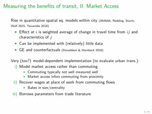
Measuring the benefits of transit, II. Market Access
Rise in quantitative spatial eq. models within city (Ahlfeldt, Redding, Sturm,Wolf 2015; Tsivanidis 2018)
I Effect at i is weighted average of change in travel time from ij andcharacteristics of j
I Can be implemented with (relatively) little dataI GE and counterfactuals (Donaldson & Hornbeck 2016)
Very (too?) model-dependent implementation (to evaluate urban trans.):i) Model market access rather than commuting
• Commuting typically not well measured well• Market access infers commuting from proximity
ii) Recover wages at place of work from commuting flows• Bakes in size/centrality
iii) Borrows parameters from trade literature
5 / 44
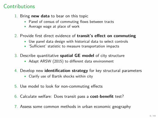
Contributions1. Bring new data to bear on this topic
• Panel of census of commuting flows between tracts• Average wage at place of work
2. Provide first direct evidence of transit’s effect on commuting• Use panel data design with historical data to select controls• ‘Sufficient’ statistic to measure transportation impacts
3. Describe quantitative spatial GE model of city structure• Adapt ARSW (2015) to different data environment
4. Develop new identification strategy for key structural parameters• Clarify use of Bartik shocks within city
5. Use model to look for non-commuting effects
6. Calculate welfare: Does transit pass a cost-benefit test?
7. Assess some common methods in urban economic geography
6 / 44
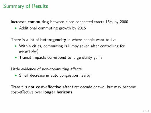
Summary of Results
Increases commuting between close-connected tracts 15% by 2000I Additional commuting growth by 2015
There is a lot of heterogeneity in where people want to liveI Within cities, commuting is lumpy (even after controlling for
geography)I Transit impacts correspond to large utility gains
Little evidence of non-commuting effectsI Small decrease in auto congestion nearby
Transit is not cost-effective after first decade or two, but may becomecost-effective over longer horizons
7 / 44
1. Data and setting
2. Transit’s effect on commuting flows (gravity)
3. Quantitative urban model with commuting
4. Structural identification and estimated elasticities
5. Non-commuting effects and welfare
6. Habituation and network returns
7. Assess quantitative economic geography models within cities
7 / 44
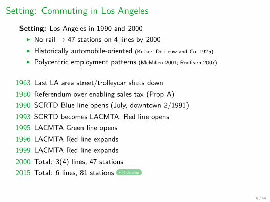
Setting: Commuting in Los AngelesSetting: Los Angeles in 1990 and 2000
I No rail → 47 stations on 4 lines by 2000I Historically automobile-oriented (Kelker, De Leuw and Co. 1925)
I Polycentric employment patterns (McMillen 2001; Redfearn 2007)
1963 Last LA area street/trolleycar shuts down1980 Referendum over enabling sales tax (Prop A)1990 SCRTD Blue line opens (July, downtown 2/1991)1993 SCRTD becomes LACMTA, Red line opens1995 LACMTA Green line opens1996 LACMTA Red line expands1999 LACMTA Red line expands2000 Total: 3(4) lines, 47 stations2015 Total: 6 lines, 81 stations Ridership
8 / 44
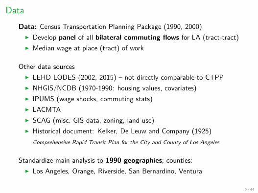
DataData: Census Transportation Planning Package (1990, 2000)
I Develop panel of all bilateral commuting flows for LA (tract-tract)I Median wage at place (tract) of work
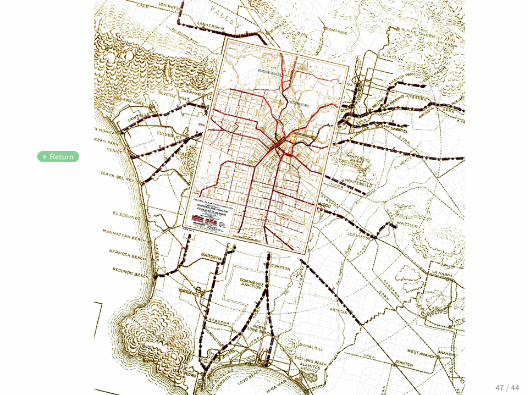
Other data sourcesI LEHD LODES (2002, 2015) – not directly comparable to CTPPI NHGIS/NCDB (1970-1990: housing values, covariates)I IPUMS (wage shocks, commuting stats)I LACMTAI SCAG (misc. GIS data, zoning, land use)I Historical document: Kelker, De Leuw and Company (1925)
Comprehensive Rapid Transit Plan for the City and County of Los Angeles
Standardize main analysis to 1990 geographies; counties:I Los Angeles, Orange, Riverside, San Bernardino, Ventura
9 / 44
1. Data and setting
2. Transit’s effect on commuting flows (gravity)
3. Quantitative urban model with commuting
4. Structural identification and estimated elasticities
5. Non-commuting effects and welfare
6. Habituation and network returns
7. Assess quantitative economic geography models within cities
9 / 44
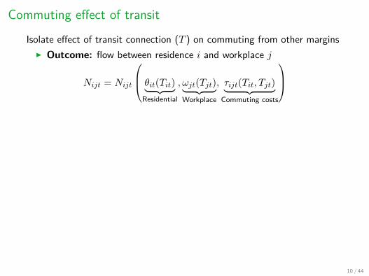
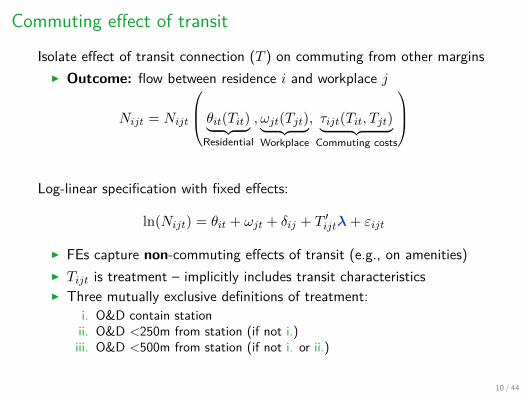
Commuting effect of transitIsolate effect of transit connection (T ) on commuting from other margins
I Outcome: flow between residence i and workplace j
Nijt = Nijt
θit(Tit)︸ ︷︷ ︸Residential
, ωjt(Tjt)︸ ︷︷ ︸Workplace
, τijt(Tit, Tjt)︸ ︷︷ ︸Commuting costs
Log-linear specification with fixed effects:
ln(Nijt) = θit + ωjt + δij + T ′ijtλ+ εijt
I FEs capture non-commuting effects of transit (e.g., on amenities)I Tijt is treatment – implicitly includes transit characteristicsI Three mutually exclusive definitions of treatment:
i. O&D contain stationii. O&D <250m from station (if not i.)
iii. O&D <500m from station (if not i. or ii.)
10 / 44
Commuting effect of transitIsolate effect of transit connection (T ) on commuting from other margins
I Outcome: flow between residence i and workplace j
Nijt = Nijt
θit(Tit)︸ ︷︷ ︸Residential
, ωjt(Tjt)︸ ︷︷ ︸Workplace
, τijt(Tit, Tjt)︸ ︷︷ ︸Commuting costs
Log-linear specification with fixed effects:
ln(Nijt) = θit + ωjt + δij + T ′ijtλ+ εijt
I FEs capture non-commuting effects of transit (e.g., on amenities)I Tijt is treatment – implicitly includes transit characteristicsI Three mutually exclusive definitions of treatment:
i. O&D contain stationii. O&D <250m from station (if not i.)iii. O&D <500m from station (if not i. or ii.)
10 / 44
i’
j’
i
j
Δ𝑻𝑻𝒊𝒊𝒊𝒊 = 𝟏𝟏
Δ𝑻𝑻𝒊𝒊′𝒊𝒊′ = 𝟎𝟎
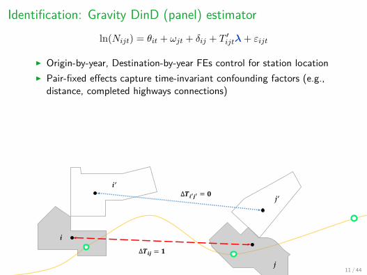
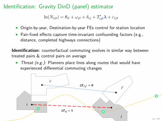
Identification: Gravity DinD (panel) estimatorln(Nijt) = θit + ωjt + δij + T ′ijtλ+ εijt
I Origin-by-year, Destination-by-year FEs control for station locationI Pair-fixed effects capture time-invariant confounding factors (e.g.,
distance, completed highways connections)
Identification: counterfactual commuting evolves in similar way betweentreated pairs & control pairs on average
I Threat (e.g.): Planners place lines along routes that would haveexperienced differential commuting changes
11 / 44
i’
j’
i
j
Δ𝑻𝑻𝒊𝒊𝒊𝒊 = 𝟏𝟏
Δ𝑻𝑻𝒊𝒊′𝒊𝒊′ = 𝟎𝟎
Identification: Gravity DinD (panel) estimatorln(Nijt) = θit + ωjt + δij + T ′ijtλ+ εijt
I Origin-by-year, Destination-by-year FEs control for station locationI Pair-fixed effects capture time-invariant confounding factors (e.g.,
distance, completed highways connections)
Identification: counterfactual commuting evolves in similar way betweentreated pairs & control pairs on average
I Threat (e.g.): Planners place lines along routes that would haveexperienced differential commuting changes
11 / 44
Controls for commuting flow DiD1) Historical subway plan (Kelker, de Leuw and Co. 1925) Map
2) Red Car routes, Pacific Electric Railroad streetcar lines3) Adjacencies (Dube, Lester, & Reich 2010)
Arguments:I Many control pairs contain a treated ‘end’ (O or D)I Similar evolution of built environment (Brooks & Lutz 2016)
I Placement: Routes connect political power centers (Elkind 2014)
I Timing: Staggered rollout based on political expediency
I Timing: Geologic shock – Ross Dress for Less blew up!
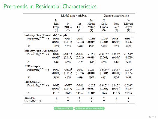
Pre-trends? Cannot directly test, but . . .I Parallel trends in pop/hous, but other tract chars. change Pre-trend 1
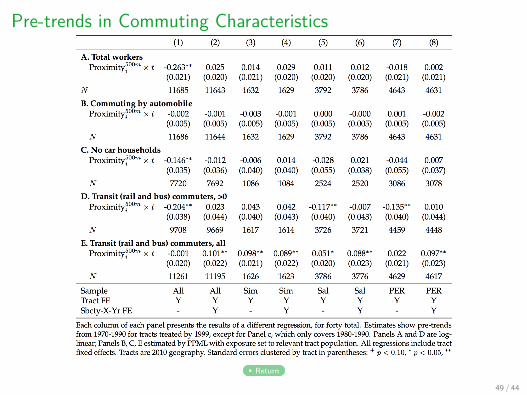
I Mostly parallel pre-trends in residential commuting Pre-trend 2
I Add Subcounty-by-Year FEs (Sbcty-x-Sbcty-x-Yr in gravity model)
12 / 44
Controls for commuting flow DiD1) Historical subway plan (Kelker, de Leuw and Co. 1925) Map
2) Red Car routes, Pacific Electric Railroad streetcar lines3) Adjacencies (Dube, Lester, & Reich 2010)
Arguments:I Many control pairs contain a treated ‘end’ (O or D)I Similar evolution of built environment (Brooks & Lutz 2016)
I Placement: Routes connect political power centers (Elkind 2014)
I Timing: Staggered rollout based on political expediencyI Timing: Geologic shock – Ross Dress for Less blew up!
Pre-trends? Cannot directly test, but . . .I Parallel trends in pop/hous, but other tract chars. change Pre-trend 1
I Mostly parallel pre-trends in residential commuting Pre-trend 2
I Add Subcounty-by-Year FEs (Sbcty-x-Sbcty-x-Yr in gravity model)
12 / 44
13 / 44
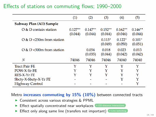
Effects of stations on commuting flows; 1990–2000
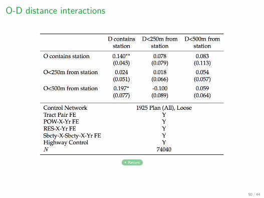
Metro increases commuting by 15% (10%) between connected tractsI Consistent across various strategies & PPMLI Effect spatially concentrated near workplaces OD-distance interactions
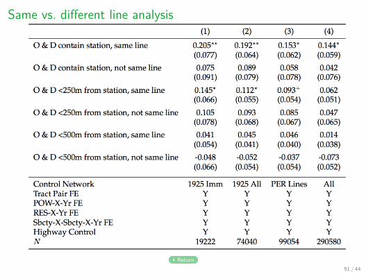
I Effect only along same line (transfers not important) Line switching
14 / 44
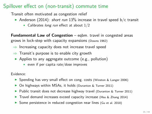
Spillover effect on (non-transit) commute timeTransit often motivated as congestion relief
I Anderson (2014): short run 13% increase in travel speed b/c transit• Calibrates long run effect at about 1/2
Fundamental Law of Congestion – eqbm. travel in congested areasgrows in lock-step with capacity expansions (Downs 1962)
⇒ Increasing capacity does not increase travel speed⇒ Transit’s purpose is to enable city growthI Applies to any aggregate outcome (e.g., pollution)
• even if per capita rate/dose improves
Evidence:I Spending has very small effect on cong. costs (Winston & Langer 2006)I On highways within MSAs, it holds (Duranton & Turner 2011)I Public transit does not decrease highway travel (Duranton & Turner 2011)I Travel demand increases exceed capacity increase (Hsu & Zhang 2014)I Some persistence in reduced congestion near lines (Gu et al. 2018)
15 / 44
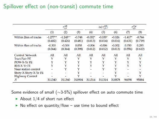
Spillover effect on (non-transit) commute time
Some evidence of small (∼3-5%) spillover effect on auto commute timeI About 1/4 of short run effectI No effect on quantity/flow – use time to bound effect
16 / 44
1. Data and setting
2. Transit’s effect on commuting flows (gravity)
3. Quantitative urban model with commuting
4. Structural identification and estimated elasticities
5. Non-commuting effects and welfare
6. Habituation and network returns
7. Assess quantitative economic geography models within cities
16 / 44
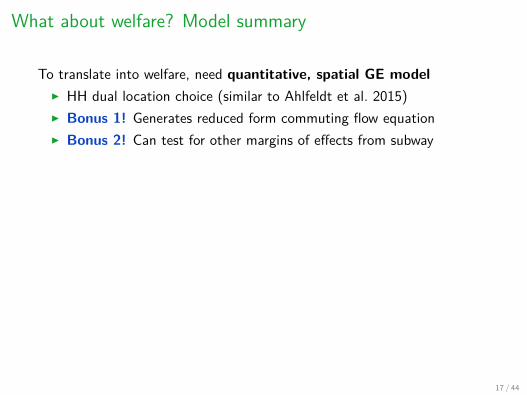
What about welfare? Model summary
To translate into welfare, need quantitative, spatial GE modelI HH dual location choice (similar to Ahlfeldt et al. 2015)I Bonus 1! Generates reduced form commuting flow equationI Bonus 2! Can test for other margins of effects from subway
Locations: N locations (census tracts) in cityI Each containing a labor market, and a housing marketI Described by exogenous supply/demand fundamentals
Agents: Three types of agents (all massless)I Workers/HHs: decide where to live and where to workI Firms: hire workersI Builders: use land & materials to produce housing
17 / 44
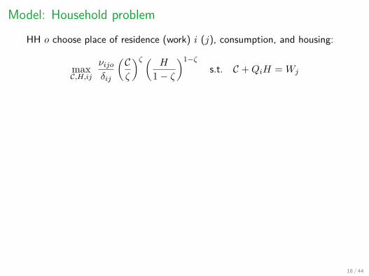
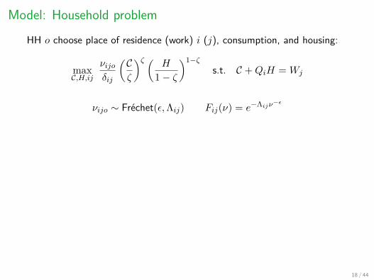
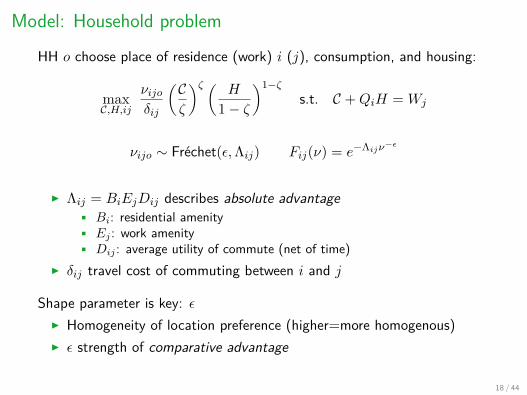
Model: Household problemHH o choose place of residence (work) i (j), consumption, and housing:
maxC,H,ij
νijoδij
(Cζ
)ζ ( H
1− ζ
)1−ζs.t. C +QiH = Wj
νijo ∼ Frechet(ε,Λij) Fij(ν) = e−Λijν−ε
I Λij = BiEjDij describes absolute advantage• Bi: residential amenity• Ej : work amenity• Dij : average utility of commute (net of time)
I δij travel cost of commuting between i and j
Shape parameter is key: εI Homogeneity of location preference (higher=more homogenous)I ε strength of comparative advantage
18 / 44
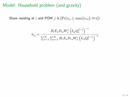
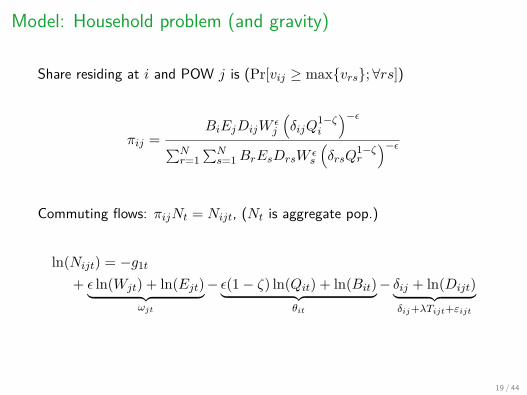
Model: Household problem (and gravity)
Share residing at i and POW j is (Pr[vij ≥ max{vrs};∀rs])
πij =BiEjDijW
εj
(δijQ
1−ζi
)−ε∑Nr=1
∑Ns=1BrEsDrsW ε
s
(δrsQ
1−ζr
)−ε
Commuting flows: πijNt = Nijt, (Nt is aggregate pop.)
ln(Nijt) = −g1t
+ ε ln(Wjt) + ln(Ejt)︸ ︷︷ ︸ωjt
− ε(1− ζ) ln(Qit) + ln(Bit)︸ ︷︷ ︸θit
− δij + ln(Dijt)︸ ︷︷ ︸δij+λTijt+εijt
19 / 44

Closing the model
Production: Cobb-Douglas in labor and landI Perfect competition, produce nationally trade goodI Multiplicatively separable productivity term Ai, can add
agglomeration, etc.
Wi = αAi(LYi /N
Yi
)1−α
Housing produced using land, materialsI Perfect competition among builders, Cobb-Douglas productionI No interaction with other land uses (restrictive zoning)
• No evidence of any zoning changesI Multiplicatively separable housing efficiency Ci
Qi = Ci(Hi/LHi )ψ
20 / 44
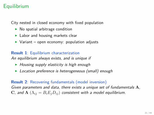
Equilibrium
City nested in closed economy with fixed populationI No spatial arbitrage conditionI Labor and housing markets clearI Variant – open economy: population adjusts
Result 1: Equilibrium characterizationAn equilibrium always exists, and is unique if
I Housing supply elasticity is high enoughI Location preference is heterogeneous (small) enough
Result 2: Recovering fundamentals (model inversion)Given parameters and data, there exists a unique set of fundamentals A,C, and Λ (Λij = BiEjDij) consistent with a model equilibrium.
21 / 44
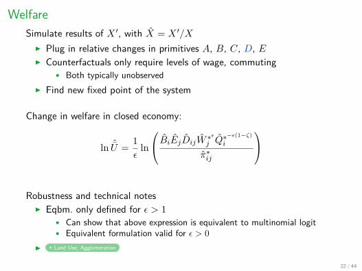
WelfareSimulate results of X ′, with X = X ′/X
I Plug in relative changes in primitives A, B, C, D, EI Counterfactuals only require levels of wage, commuting
• Both typically unobservedI Find new fixed point of the system
Change in welfare in closed economy:
ln ˆU = 1ε
ln
BiEjDijW∗εj Q
∗−ε(1−ζ)i
π∗ij
Robustness and technical notesI Eqbm. only defined for ε > 1
• Can show that above expression is equivalent to multinomial logit• Equivalent formulation valid for ε > 0
I Land Use; Agglomeration
22 / 44

1. Data and setting
2. Transit’s effect on commuting flows (gravity)
3. Quantitative urban model with commuting
4. Structural identification and estimated elasticities
5. Non-commuting effects and welfare
6. Habituation and network returns
7. Assess quantitative economic geography models within cities
22 / 44
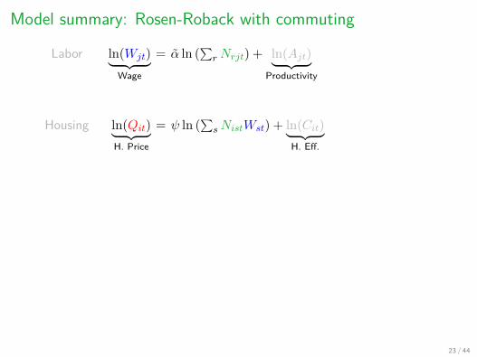
Model summary: Rosen-Roback with commuting
Labor ln(Wjt)︸ ︷︷ ︸Wage
= α ln (∑rNrjt) + ln(Ajt)︸ ︷︷ ︸
Productivity
Commut. ln(Nijt)︸ ︷︷ ︸Flow
= ε ln(Wjt) + εζ ln(Qit) + δij + ln(BitEjtDijt)︸ ︷︷ ︸Commuting and Amenities
Housing ln(Qit)︸ ︷︷ ︸H. Price
= ψ ln (∑sNistWst) + ln(Cit)︸ ︷︷ ︸
H. Eff.
Describes1. Slopes: ε, ψ, εζ, α
• Local elasticities2. Shifts: Changes to primitivesA, B, C, D, E
• Effects of transit
Q
H
𝐻𝐷
𝐻𝑆
𝛽 = ∆𝑄𝐸
∆𝐶 ∆𝐵
𝜓
−𝜁
23 / 44
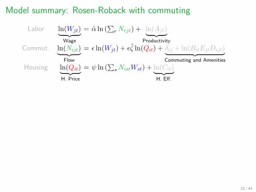
Model summary: Rosen-Roback with commuting
Labor ln(Wjt)︸ ︷︷ ︸Wage
= α ln (∑rNrjt) + ln(Ajt)︸ ︷︷ ︸
ProductivityCommut. ln(Nijt)︸ ︷︷ ︸
Flow
= ε ln(Wjt) + εζ ln(Qit) + δij + ln(BitEjtDijt)︸ ︷︷ ︸Commuting and Amenities
Housing ln(Qit)︸ ︷︷ ︸H. Price
= ψ ln (∑sNistWst) + ln(Cit)︸ ︷︷ ︸
H. Eff.
Describes1. Slopes: ε, ψ, εζ, α
• Local elasticities2. Shifts: Changes to primitivesA, B, C, D, E
• Effects of transit
Q
H
𝐻𝐷
𝐻𝑆
𝛽 = ∆𝑄𝐸
∆𝐶 ∆𝐵
𝜓
−𝜁
23 / 44
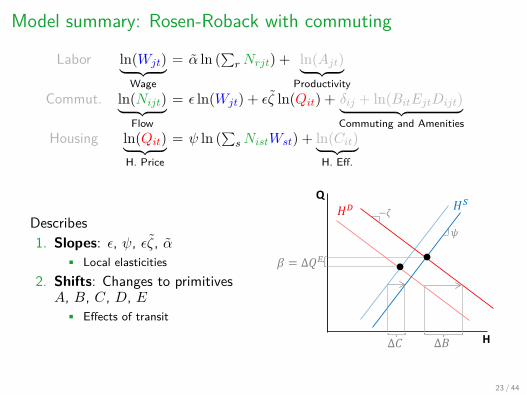
Model summary: Rosen-Roback with commuting
Labor ln(Wjt)︸ ︷︷ ︸Wage
= α ln (∑rNrjt) + ln(Ajt)︸ ︷︷ ︸
ProductivityCommut. ln(Nijt)︸ ︷︷ ︸
Flow
= ε ln(Wjt) + εζ ln(Qit) + δij + ln(BitEjtDijt)︸ ︷︷ ︸Commuting and Amenities
Housing ln(Qit)︸ ︷︷ ︸H. Price
= ψ ln (∑sNistWst) + ln(Cit)︸ ︷︷ ︸
H. Eff.
Describes1. Slopes: ε, ψ, εζ, α
• Local elasticities2. Shifts: Changes to primitivesA, B, C, D, E
• Effects of transit
Q
H
𝐻𝐷
𝐻𝑆
𝛽 = ∆𝑄𝐸
∆𝐶 ∆𝐵
𝜓
−𝜁
23 / 44
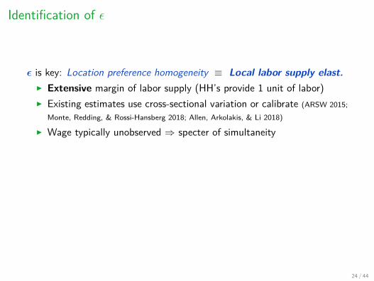
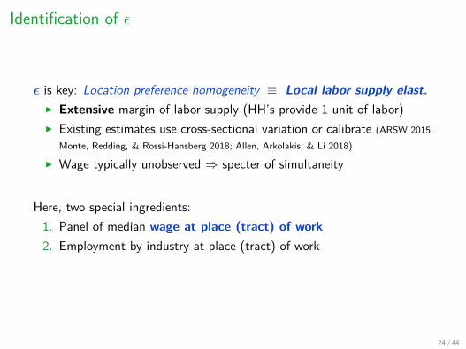
Identification of ε
ε is key: Location preference homogeneity ≡ Local labor supply elast.I Extensive margin of labor supply (HH’s provide 1 unit of labor)I Existing estimates use cross-sectional variation or calibrate (ARSW 2015;
Monte, Redding, & Rossi-Hansberg 2018; Allen, Arkolakis, & Li 2018)
I Wage typically unobserved ⇒ specter of simultaneity
Here, two special ingredients:1. Panel of median wage at place (tract) of work2. Employment by industry at place (tract) of work
24 / 44
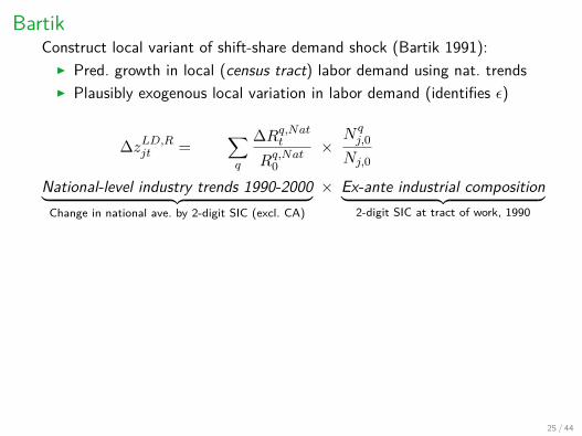
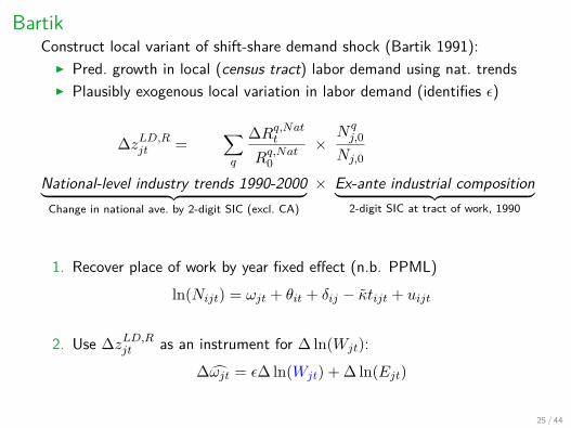
BartikConstruct local variant of shift-share demand shock (Bartik 1991):
I Pred. growth in local (census tract) labor demand using nat. trendsI Plausibly exogenous local variation in labor demand (identifies ε)
∆zLD,Rjt =∑q
∆Rq,Natt
Rq,Nat0×
N qj,0
Nj,0
National-level industry trends 1990-2000︸ ︷︷ ︸Change in national ave. by 2-digit SIC (excl. CA)
× Ex-ante industrial composition︸ ︷︷ ︸2-digit SIC at tract of work, 1990
1. Recover place of work by year fixed effect (n.b. PPML)ln(Nijt) = ωjt + θit + δij − κtijt + uijt
2. Use ∆zLD,Rjt as an instrument for ∆ ln(Wjt):∆ωjt = ε∆ ln(Wjt) + ∆ ln(Ejt)
25 / 44
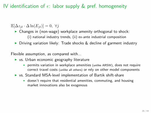
IV identification of ε: labor supply & pref. homogeneity
E[∆zjt ·∆ ln(Ejt)] = 0, ∀jI Changes in (non-wage) workplace amenity orthogonal to shock:
(i) national industry trends, (ii) ex-ante industrial compositionI Driving variation likely: Trade shocks & decline of garment industry
Flexible assumption, as compared with...I vs. Urban economic geography literature
• permits variation in workplace amenities (unlike ARSW), does not requirecorrect travel costs (unlike all others) or rely on other model components
I vs. Standard MSA-level implementation of Bartik shift-share• doesn’t require that residential amenities, commuting, and housing
market innovations also be exogenous
26 / 44
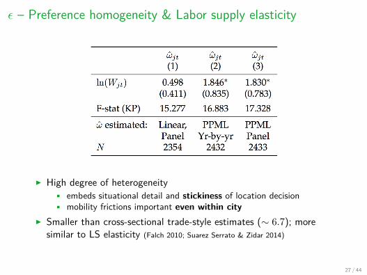
ε – Preference homogeneity & Labor supply elasticity
I High degree of heterogeneity• embeds situational detail and stickiness of location decision• mobility frictions important even within city
I Smaller than cross-sectional trade-style estimates (∼ 6.7); moresimilar to LS elasticity (Falch 2010; Suarez Serrato & Zidar 2014)
27 / 44
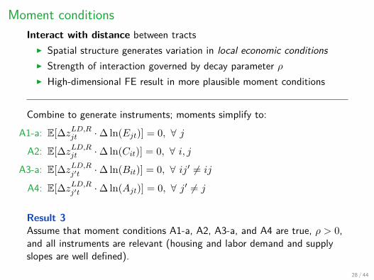
Moment conditionsInteract with distance between tracts
I Spatial structure generates variation in local economic conditionsI Strength of interaction governed by decay parameter ρI High-dimensional FE result in more plausible moment conditions
Combine to generate instruments; moments simplify to:A1-a: E[∆zLD,Rjt ·∆ ln(Ejt)] = 0, ∀ j
A2: E[∆zLD,Rjt ·∆ ln(Cit)] = 0, ∀ i, j
A3-a: E[∆zLD,Rj′t ·∆ ln(Bit)] = 0, ∀ ij′ 6= ij
A4: E[∆zLD,Rj′t ·∆ ln(Ajt)] = 0, ∀ j′ 6= j
Result 3Assume that moment conditions A1-a, A2, A3-a, and A4 are true, ρ > 0,and all instruments are relevant (housing and labor demand and supplyslopes are well defined).
28 / 44
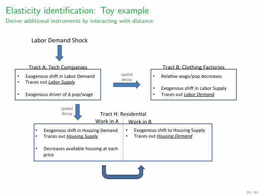
• Exogenousshi,inLaborDemand• TracesoutLaborSupply
• ExogenousdriverofΔpop/wage
LaborDemandShock
TractA:TechCompanies
TractH:ResidenDal
• Exogenousshi,inHousingDemand• TracesoutHousingSupply
• Decreasesavailablehousingateachprice
• Exogenousshi,toHousingSupply• TracesoutHousingDemand
• RelaDvewage/popdecreases
• Exogenousshi,inLaborSupply• TracesoutLaborDemand
TractB:ClothingFactories
WorkinA WorkinB
spaDaldecay
spaDaldecay
Elasticity identification: Toy exampleDerive additional instruments by interacting with distance
29 / 44
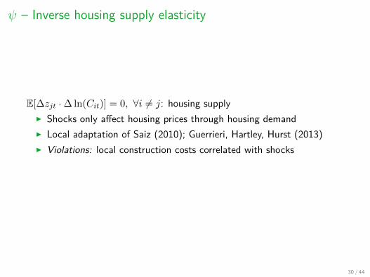
ψ – Inverse housing supply elasticity
E[∆zjt ·∆ ln(Cit)] = 0, ∀i 6= j: housing supplyI Shocks only affect housing prices through housing demandI Local adaptation of Saiz (2010); Guerrieri, Hartley, Hurst (2013)I Violations: local construction costs correlated with shocks
30 / 44
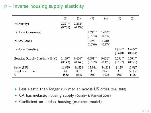
ψ – Inverse housing supply elasticity
I Less elastic than longer run median across US cities (Saiz 2010)
I CA has inelastic housing supply (Quigley & Raphael 2005)
I Coefficient on land ≈ housing (matches model)
31 / 44
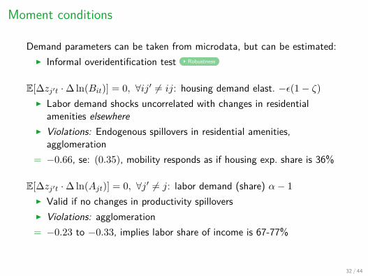
Moment conditions
Demand parameters can be taken from microdata, but can be estimated:I Informal overidentification test Robustness
E[∆zj′t ·∆ ln(Bit)] = 0, ∀ij′ 6= ij: housing demand elast. −ε(1− ζ)I Labor demand shocks uncorrelated with changes in residential
amenities elsewhereI Violations: Endogenous spillovers in residential amenities,
agglomeration= −0.66, se: (0.35), mobility responds as if housing exp. share is 36%
E[∆zj′t ·∆ ln(Ajt)] = 0, ∀j′ 6= j: labor demand (share) α− 1I Valid if no changes in productivity spilloversI Violations: agglomeration= −0.23 to −0.33, implies labor share of income is 67-77%
32 / 44
1. Data and setting
2. Transit’s effect on commuting flows (gravity)
3. Quantitative urban model with commuting
4. Structural identification and estimated elasticities
5. Non-commuting effects and welfare
6. Habituation and network returns
7. Assess quantitative economic geography models within cities
32 / 44
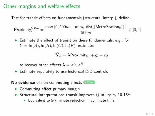
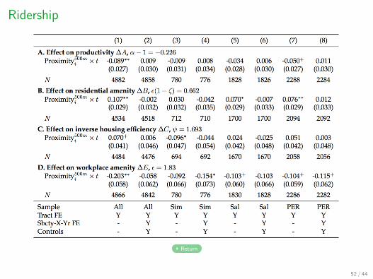
Other margins and welfare effects
Test for transit effects on fundamentals (structural interp.), define:
Proximity500mi = max{0, 500m−mink{disti(MetroStationk)}}
500m ∈ [0, 1]
I Estimate the effect of transit on these fundamentals, e.g., forY = ln(A), ln(B), ln(C), ln(E), estimate:
Yit = λProximityit + ςi + εit
to recover other effects λ = λA, λB, . . .
I Estimate separately to use historical DiD controls
No evidence of non-commuting effects Tables
I Commuting effect primary marginI Structural interpretation: transit improves ij utility by 10-15%
• Equivalent to 5-7 minute reduction in commute time
33 / 44
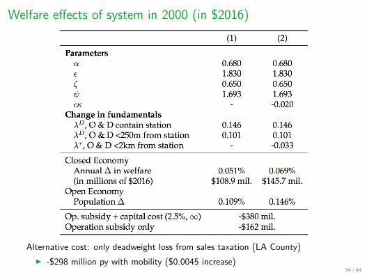
Welfare effects of system in 2000 (in $2016)
Alternative cost: only deadweight loss from sales taxation (LA County)I -$298 million py with mobility ($0.0045 increase)
34 / 44
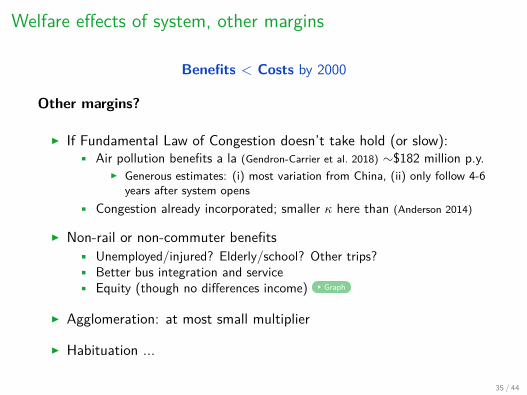
Welfare effects of system, other margins
Benefits < Costs by 2000
Other margins?
I If Fundamental Law of Congestion doesn’t take hold (or slow):• Air pollution benefits a la (Gendron-Carrier et al. 2018) ∼$182 million p.y.
I Generous estimates: (i) most variation from China, (ii) only follow 4-6years after system opens
• Congestion already incorporated; smaller κ here than (Anderson 2014)
I Non-rail or non-commuter benefits• Unemployed/injured? Elderly/school? Other trips?• Better bus integration and service• Equity (though no differences income) Graph
I Agglomeration: at most small multiplier
I Habituation ...
35 / 44
1. Data and setting
2. Transit’s effect on commuting flows (gravity)
3. Quantitative urban model with commuting
4. Structural identification and estimated elasticities
5. Non-commuting effects and welfare
6. Habituation and network returns
7. Assess quantitative economic geography models within cities
35 / 44
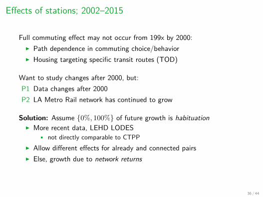
Effects of stations; 2002–2015
Full commuting effect may not occur from 199x by 2000:I Path dependence in commuting choice/behaviorI Housing targeting specific transit routes (TOD)
Want to study changes after 2000, but:P1 Data changes after 2000P2 LA Metro Rail network has continued to grow
Solution: Assume {0%, 100%} of future growth is habituationI More recent data, LEHD LODES
• not directly comparable to CTPPI Allow different effects for already and connected pairsI Else, growth due to network returns
36 / 44
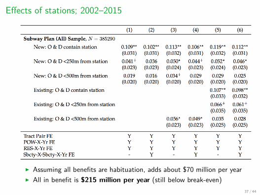
Effects of stations; 2002–2015
I Assuming all benefits are habituation, adds about $70 million per yearI All in benefit is $215 million per year (still below break-even)
37 / 44
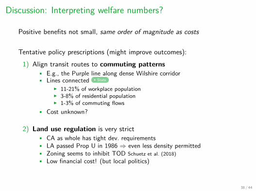
Discussion: Interpreting welfare numbers?
Positive benefits not small, same order of magnitude as costs
Tentative policy prescriptions (might improve outcomes):1) Align transit routes to commuting patterns
• E.g., the Purple line along dense Wilshire corridor• Lines connected Stats
I 11-21% of workplace populationI 3-8% of residential populationI 1-3% of commuting flows
• Cost unknown?
2) Land use regulation is very strict• CA as whole has tight dev. requirements• LA passed Prop U in 1986 ⇒ even less density permitted• Zoning seems to inhibit TOD Schuetz et al. (2018)• Low financial cost! (but local politics)
38 / 44
1. Data and setting
2. Transit’s effect on commuting flows (gravity)
3. Quantitative urban model with commuting
4. Structural identification and estimated elasticities
5. Non-commuting effects and welfare
6. Habituation and network returns
7. Assess quantitative economic geography models within cities
38 / 44
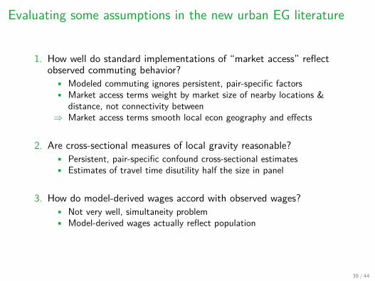
Evaluating some assumptions in the new urban EG literature
1. How well do standard implementations of “market access” reflectobserved commuting behavior?
• Modeled commuting ignores persistent, pair-specific factors• Market access terms weight by market size of nearby locations &
distance, not connectivity between⇒ Market access terms smooth local econ geography and effects
2. Are cross-sectional measures of local gravity reasonable?• Persistent, pair-specific confound cross-sectional estimates• Estimates of travel time disutility half the size in panel
3. How do model-derived wages accord with observed wages?• Not very well, simultaneity problem• Model-derived wages actually reflect population
39 / 44
1. Market AccessMarket access terms summarize trade-cost weighted size of market:
MAi =∑s
e−κτisYs
where Ys is other market size (population, GDP, total consumer exp.)
Contribution of is and is′ equivalent if Ys = Ys′ and τis = τis′I What if observe greater flows between is and is′? Stronger
connection? Random noise? Now what if is persistent? 0s?
“Standard approach” in urban EG:i) Use travel survey to estimate κii) Scrape travel times and travel times with transit changeiii) Predict changes in commuting from i) and ii)iv) Use changes in market access implied by iii)
40 / 44
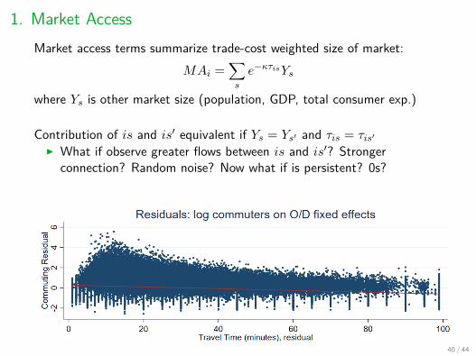
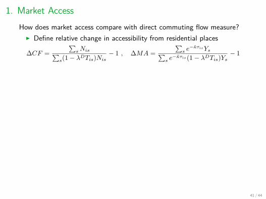
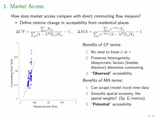
1. Market AccessHow does market access compare with direct commuting flow measure?
I Define relative change in accessibility from residential places
∆CF =∑sNis∑
s(1− λDTis)Nis− 1 , ∆MA =
∑s e
−κτisYs∑s e
−κτis(1− λDTis)Ys− 1
Benefits of CF terms:1. No need to know κ or τ2. Preserves heterogeneity;
idiosyncratic factors (besidesdistance) determine commuting
3. “Observed” accessibilityBenefits of MA terms:
1. Can scrape/model travel time data2. Smooths spatial economy, like
spatial weights? (Sp. E/metrics)3. “Potential” accessibility
41 / 44
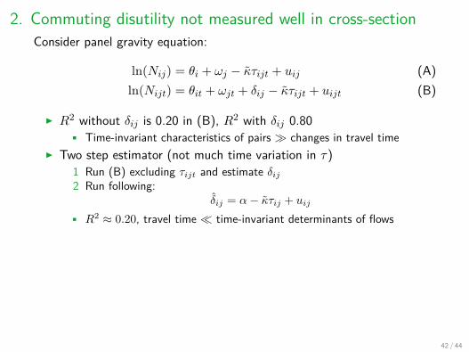
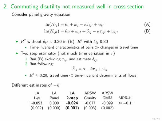
2. Commuting disutility not measured well in cross-sectionConsider panel gravity equation:
ln(Nij) = θi + ωj − κτijt + uij (A)ln(Nijt) = θit + ωjt + δij − κτijt + uijt (B)
I R2 without δij is 0.20 in (B), R2 with δij 0.80• Time-invariant characteristics of pairs � changes in travel time
I Two step estimator (not much time variation in τ)1 Run (B) excluding τijt and estimate δij2 Run following:
δij = α− κτij + uij
• R2 ≈ 0.20, travel time � time-invariant determinants of flows
Different estimates of −κ:LA LA LA ARSW ARSW1-yr Panel 2-step Gravity GMM MRR-H
-0.053 0.000 -0.024 -0.077 -0.099 ≈ −0.1(0.002) (0.000) (0.001) (0.003) (0.002)
42 / 44
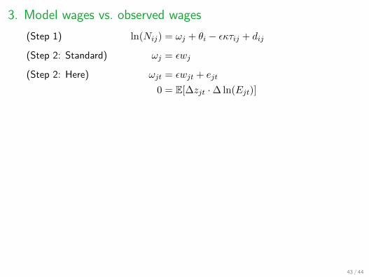
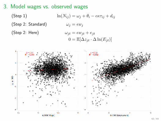
3. Model wages vs. observed wagesln(Nij) = ωj + θi − εκτij + dij(Step 1)
ωj = εwj(Step 2: Standard)
ωjt = εwjt + ejt(Step 2: Here)0 = E[∆zjt ·∆ ln(Ejt)]
43 / 44
3. Model wages vs. observed wagesln(Nij) = ωj + θi − εκτij + dij(Step 1)
ωj = εwj(Step 2: Standard)
ωjt = εwjt + ejt(Step 2: Here)0 = E[∆zjt ·∆ ln(Ejt)]
43 / 44
Summary
Develop new data sources to estimate effects of LA Metro:I Positive effect on commuting between connected tractsI Little adjustment on other margins
Carefully identify elasticities that populate econ. geo. modelI New identification strategy based on tract-level shift-share instrumentI Local stickiness, limited mobility even within cityI Permits more retention of unmodeled heterogeneity
Calculate welfare benefits of LA MetroI Significant benefits, but costs are largerI Even after 25 years...
Critically examine urban EG modeling
44 / 44
Thank you
Los
Ange
les
Riv
er
Los Angeles River Univers
al City
/Stu
dio City
Hollywood/V
ine
Hollywood/H
ighland
Univers
al City
/Stu
dio City
Balboa
Canoga
De Soto
Pierce Colle
ge
Tam
pa
Reseda
Civic Ctr/
Civic Ctr/
Civic Ctr/
Civic Ctr/
Grand
Grand
Grand
Grand
ParkParkParkPark
Westlake/M
acArthur P
ark
Warner Ctr
Roscoe
Pico/A
liso
Mariach
i Pla
za
Long Beach
Bl
Pacific Av
Artesia
Del Amo
DowntownLong Beach
Civic Ctr/
Grand
Park
Allen
LakeSierr
a Madre
Villa
Arcadia
Monrovia
Duarte/C
ity of H
ope
Irwindale
Azusa D
owntown
APU/Citr
us College
Lincoln/Cypress
Heritage Sq
Southwest Museum
Highland Park
Fillmore
Del Mar
Memorial Park
South Pasadena
Westlake/M
acArthur P
ark
Wils
hire/V
ermont
Pershing
Chinatown
Union Station
Chinatown
Square
7th St/Metro CtrPico
LATTC/OrthoInstitute
Jeffers
on/USC
Union Station
LAX FlyAwayAmtrak & MetrolinkLAX FlyAwayAmtrak & Metrolink
Metrolin
k
Sherman Way
Warner Ctr
Roscoe
Nordhoff
Chatsworth
Hollywood/W
estern
Vermont/S
anta M
onicaHolly
wood/Weste
rn
Hollywood/V
ine
Hollywood/H
ighlandNorth
Holly
wood
Balboa
Woodley
Sepulveda
Van Nuys
Woodman
Valley Colle
ge
Laurel C
anyon
Canoga
De Soto
Pierce Colle
ge
Tam
pa
Reseda
Vermont/B
everly
Vermont/S
anta M
onica
Vermont/S
unset
Vermont/S
unset
Amtrak & Metrolink
Soto
Indiana
Maravill
a
East LA Civic
Ctr
Atlantic
El Monte
Cal Sta
te LA
LAC+USC Medica
l Ctr
Pico/A
liso
Little
Tokyo
/
Little
Tokyo
/
Arts D
ist
Mariach
i Pla
za
Wils
hire/
Normandie
Wils
hire/W
estern
ExpoPark
/USC
Expo/Verm
ont
Expo/Weste
rn
Expo/Cre
nshaw
Farmdale
Expo/La B
rea
La Cienega/Jeffers
on
Culver C
ity
Palms
Westwood/R
ancho Park
Expo/Sepulve
da
Expo/Bundy
26th St/B
ergam
ot
17th
St/SMC
Downtown Santa
Monica
Mariposa
El Segundo
Douglas
Redondo Beach
37th St/USC
Rosecrans
Harbor
Carson
Pacific CoastHwy
GatewayTransit Ctr
Long Beach
Bl
Avalon
Vermont/
Athens
Crenshaw
Hawthorn
e/Lennox
Aviation/L
AX
Lakewood Bl
Norwalk
Slauson
Manchester
Harbor F
wy
CRENSHAW/
PURPLE LINE EXTENSION
REGIONAL CONNECTOR
LAX LINE
LAX
5th St
1st St
Pacific Av
Washington
Vernon
Slauson
Florence
Firestone
Compton
Artesia
Del Amo
Wardlow
Willow St
Pacific Coast Hwy
Anaheim St
103rd St/
Willowbrook/Rosa Parks
DowntownLong Beach
Grand/LATTC
San Pedro St
Watts Towers
SAN FERNANDO VALLEY
SAN GABRIEL VALLEY
EASTSIDE
SOUTH BAY
GATEWAY CITIES
DOWNTOWNLA
SOUTH LA
WESTSIDE
CENTRAL LA
North Hollywood to Union Station
Metro Rail
Wilshire/Western to Union StationPurple Line
Blue Line
Expo Line
Orange Line
Amtrak
LAX FlyAway
Metrolink
Metro Busway
Regional Rail
Green Line
Gold Line
Downtown LA to Long Beach
Downtown LA to Santa Monica
Redondo Beach to Norwalk
East Los Angeles to Azusa
Silver Line
Chatsworth to North Hollywood
San Pedro to El Monte
amtrak.com
metrolinktrains.com
lawa.org/flyaway
Street Service in Downtown LAand San Pedro
MAY 2016 Subject to Change
Airport Shuttle
Rail Station
StationTransfer
Busway
Statio
n
UNDERCONSTRUCTION
Busway StreetService
Red Line
metro.netMetro Rail & Busway
16-1
417
©20
16 L
ACM
TA
MAY 2016 Subject to Change
44 / 44

Extra slides
45 / 44
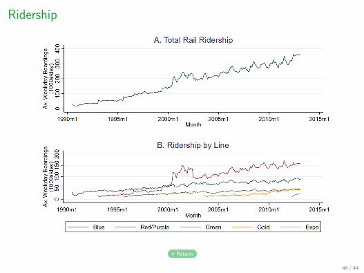
Ridership
Return
46 / 44
Return
47 / 44
Pre-trends in Residential Characteristics
Return (DiD) Return (Fundamentals)
48 / 44
Pre-trends in Commuting Characteristics
Return
49 / 44
O-D distance interactions
Return
50 / 44
Same vs. different line analysis
Return51 / 44
Ridership
Return
52 / 44
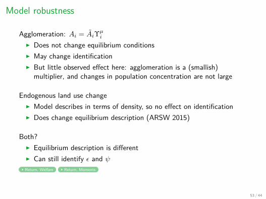
Model robustness
Agglomeration: Ai = AiΥµi
I Does not change equilibrium conditionsI May change identificationI But little observed effect here: agglomeration is a (smallish)
multiplier, and changes in population concentration are not large
Endogenous land use changeI Model describes in terms of density, so no effect on identificationI Does change equilibrium description (ARSW 2015)
Both?I Equilibrium description is differentI Can still identify ε and ψReturn, Welfare Return, Moments
53 / 44
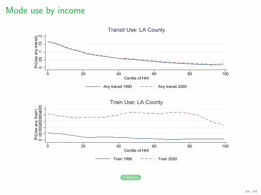
Mode use by income
0.0
5.1
.15
.2P
r(U
se a
ny tr
ansi
t)
0 20 40 60 80 100Centile of HHI
Any transit 1990 Any transit 2000
Transit Use: LA County
0.0
01.0
02.0
03.0
04.0
05P
r(U
se a
ny 't
rain
')
0 20 40 60 80 100Centile of HHI
Train 1990 Train 2000
Train Use: LA County
Return
54 / 44
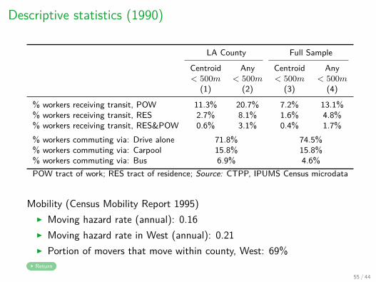
Descriptive statistics (1990)
LA County Full Sample
Centroid Any Centroid Any< 500m < 500m < 500m < 500m
(1) (2) (3) (4)
% workers receiving transit, POW 11.3% 20.7% 7.2% 13.1%% workers receiving transit, RES 2.7% 8.1% 1.6% 4.8%% workers receiving transit, RES&POW 0.6% 3.1% 0.4% 1.7%% workers commuting via: Drive alone 71.8% 74.5%% workers commuting via: Carpool 15.8% 15.8%% workers commuting via: Bus 6.9% 4.6%POW tract of work; RES tract of residence; Source: CTPP, IPUMS Census microdata
Mobility (Census Mobility Report 1995)I Moving hazard rate (annual): 0.16I Moving hazard rate in West (annual): 0.21I Portion of movers that move within county, West: 69%Return
55 / 44
Recommended