1
Charging Current in Long Lines and High
Voltage Cables –
Protection Application Considerations
Yiyan Xue, American Electric Power, Inc.
Dale Finney and Bin Le, Schweitzer Engineering Laboratories, Inc.
.
Abstract—In the analysis of power line protection behavior,
the series impedance of the lumped parameter line model is often
sufficient because the impact of the shunt capacitance is not
significant. However when long transmission overhead lines or
underground cables are present in the system, the effects of the
charging current caused by the shunt capacitance need to be
considered. This current flows onto the protected line or cable
from all terminals. Its impacts are present during normal
operation and during system transients. Due to the homogeneity
of the line impedances, the charging currents can be relatively
equal in each phase in the steady state. Thus the negative and
zero sequence components will be small – an advantage when
applying relays that operate for sequence components. However,
the charging current during line energization, internal, and
external faults will differ from steady-state values. This paper
explores the impact of charging current on the various types of
protection employed to protect line and cable circuits. It reviews
methods used to mitigate the effects of charging current and
provides general guidance on settings.
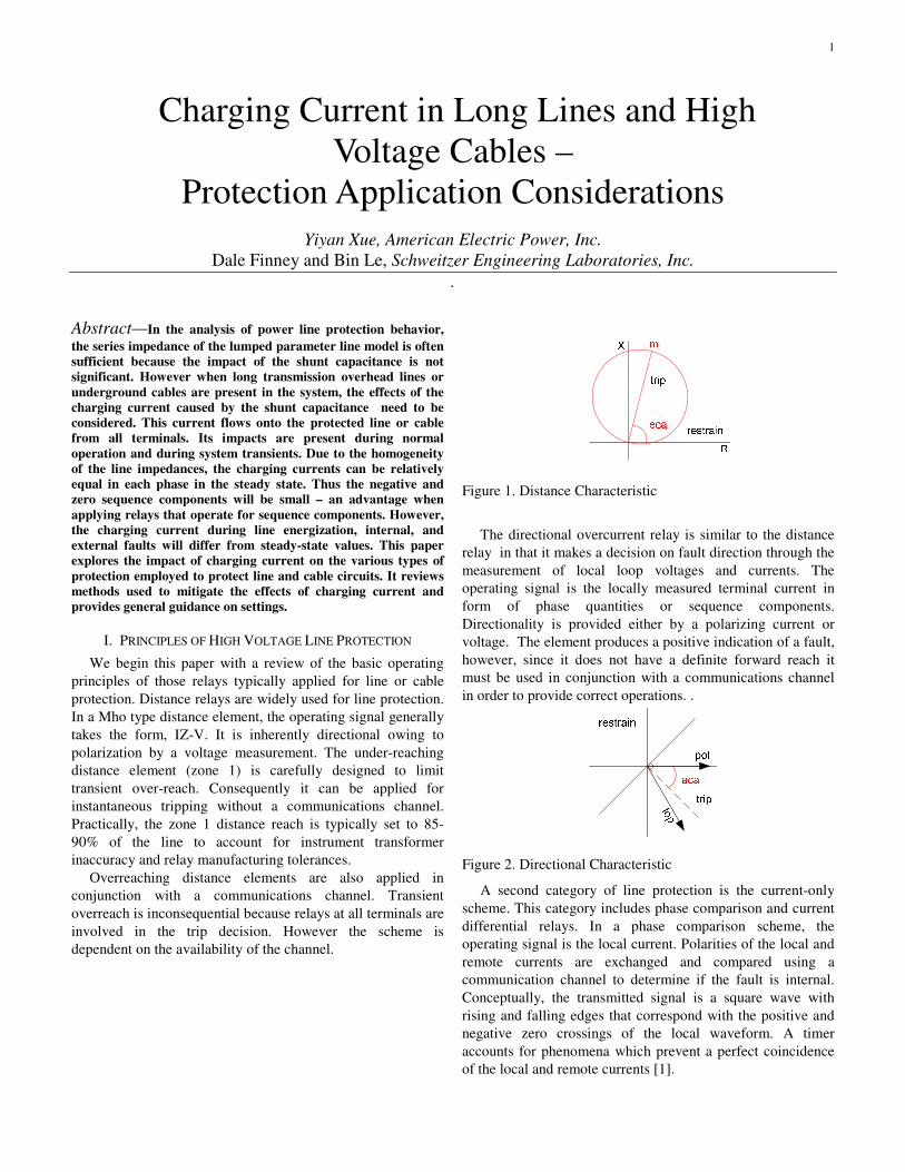
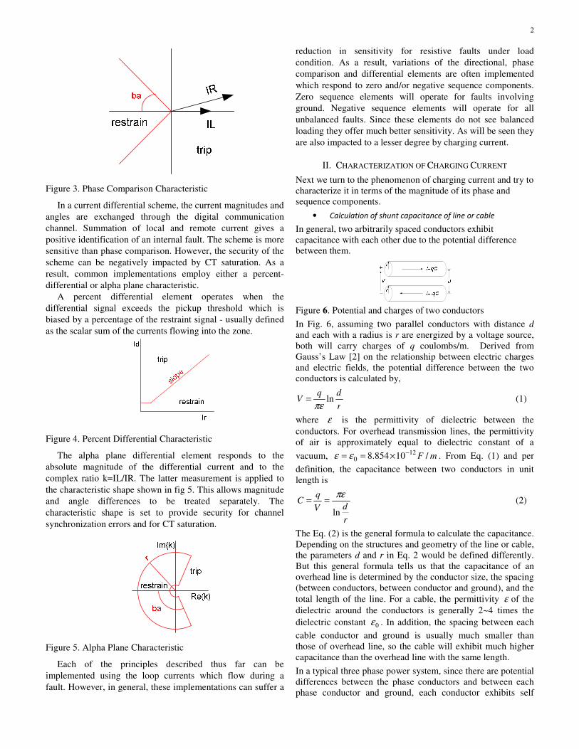
I. PRINCIPLES OF HIGH VOLTAGE LINE PROTECTION
We begin this paper with a review of the basic operating
principles of those relays typically applied for line or cable
protection. Distance relays are widely used for line protection.
In a Mho type distance element, the operating signal generally
takes the form, IZ-V. It is inherently directional owing to
polarization by a voltage measurement. The under-reaching
distance element (zone 1) is carefully designed to limit
transient over-reach. Consequently it can be applied for
instantaneous tripping without a communications channel.
Practically, the zone 1 distance reach is typically set to 85-
90% of the line to account for instrument transformer
inaccuracy and relay manufacturing tolerances.
Overreaching distance elements are also applied in
conjunction with a communications channel. Transient
overreach is inconsequential because relays at all terminals are
involved in the trip decision. However the scheme is
dependent on the availability of the channel.
Figure 1. Distance Characteristic
The directional overcurrent relay is similar to the distance
relay in that it makes a decision on fault direction through the
measurement of local loop voltages and currents. The
operating signal is the locally measured terminal current in
form of phase quantities or sequence components.
Directionality is provided either by a polarizing current or
voltage. The element produces a positive indication of a fault,
however, since it does not have a definite forward reach it
must be used in conjunction with a communications channel
in order to provide correct operations. .
Figure 2. Directional Characteristic
A second category of line protection is the current-only
scheme. This category includes phase comparison and current
differential relays. In a phase comparison scheme, the
operating signal is the local current. Polarities of the local and
remote currents are exchanged and compared using a
communication channel to determine if the fault is internal.
Conceptually, the transmitted signal is a square wave with
rising and falling edges that correspond with the positive and
negative zero crossings of the local waveform. A timer
accounts for phenomena which prevent a perfect coincidence
of the local and remote currents [1].
2
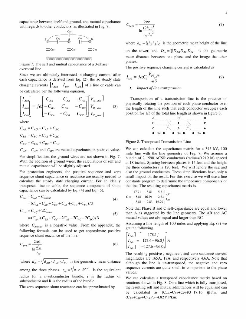
Figure 3. Phase Comparison Characteristic
In a current differential scheme, the current magnitudes and
angles are exchanged through the digital communication
channel. Summation of local and remote current gives a
positive identification of an internal fault. The scheme is more
sensitive than phase comparison. However, the security of the
scheme can be negatively impacted by CT saturation. As a
result, common implementations employ either a percent-
differential or alpha plane characteristic.
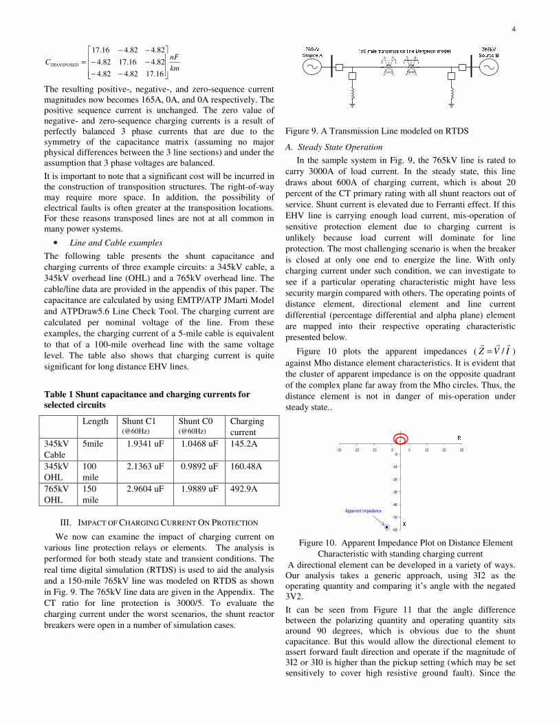
A percent differential element operates when the
differential signal exceeds the pickup threshold which is
biased by a percentage of the restraint signal - usually defined
as the scalar sum of the currents flowing into the zone.
Figure 4. Percent Differential Characteristic
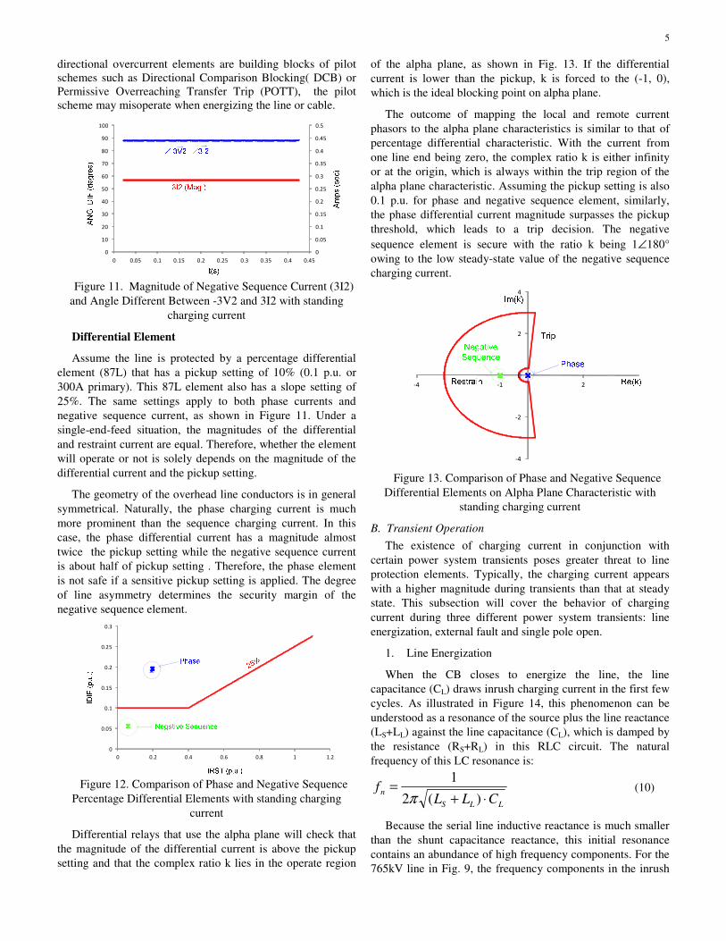
The alpha plane differential element responds to the
absolute magnitude of the differential current and to the
complex ratio k=IL/IR. The latter measurement is applied to
the characteristic shape shown in fig 5. This allows magnitude
and angle differences to be treated separately. The
characteristic shape is set to provide security for channel
synchronization errors and for CT saturation.
Figure 5. Alpha Plane Characteristic
Each of the principles described thus far can be
implemented using the loop currents which flow during a
fault. However, in general, these implementations can suffer a
reduction in sensitivity for resistive faults under load
condition. As a result, variations of the directional, phase
comparison and differential elements are often implemented
which respond to zero and/or negative sequence components.
Zero sequence elements will operate for faults involving
ground. Negative sequence elements will operate for all
unbalanced faults. Since these elements do not see balanced
loading they offer much better sensitivity. As will be seen they
are also impacted to a lesser degree by charging current.
II. CHARACTERIZATION OF CHARGING CURRENT
Next we turn to the phenomenon of charging current and try to
characterize it in terms of the magnitude of its phase and
sequence components.
• Calculation of shunt capacitance of line or cable
In general, two arbitrarily spaced conductors exhibit
capacitance with each other due to the potential difference
between them.
Figure 6. Potential and charges of two conductors
In Fig. 6, assuming two parallel conductors with distance d
and each with a radius is r are energized by a voltage source,
both will carry charges of q coulombs/m. Derived from
Gauss’s Law [2] on the relationship between electric charges
and electric fields, the potential difference between the two
conductors is calculated by,
r
dqV ln
πε= (1)
where ε is the permittivity of dielectric between the
conductors. For overhead transmission lines, the permittivity
of air is approximately equal to dielectric constant of a
vacuum, mF /10854.8 120
−×== εε . From Eq. (1) and per
definition, the capacitance between two conductors in unit
length is
r
dV
qC
ln
πε== (2)
The Eq. (2) is the general formula to calculate the capacitance.
Depending on the structures and geometry of the line or cable,
the parameters d and r in Eq. 2 would be defined differently.
But this general formula tells us that the capacitance of an
overhead line is determined by the conductor size, the spacing
(between conductors, between conductor and ground), and the
total length of the line. For a cable, the permittivity ε of the
dielectric around the conductors is generally 2~4 times the
dielectric constant 0ε . In addition, the spacing between each
cable conductor and ground is usually much smaller than
those of overhead line, so the cable will exhibit much higher
capacitance than the overhead line with the same length.
In a typical three phase power system, since there are potential
differences between the phase conductors and between each
phase conductor and ground, each conductor exhibits self
3
capacitance between itself and ground, and mutual capacitance
with regards to other conductors, as illustrated in Fig. 7.
AB C
CBC
CAB CAC
CBG CAG CCG
Figure 7. The self and mutual capacitance of a 3-phase
overhead line
Since we are ultimately interested in charging current, after
each capacitance is derived from Eq. (2), the ac steady state
charging currents [ ]CchBchAch III of a line or cable can
be calculated per the following equation,
−−
−−
−−
=
aveC
aveB
aveA
CCCBCA
BCBBBA
ACABAA
Cch
Bch
Ach
V
V
V
CCC
CCC
CCC
j
I
I
I
_
_
_
ω (3)
where
ACABAGAA CCCC ++=
BCABBGBB CCCC ++=
ACBCCGCC CCCC ++=
ABC , ACC and BCC are mutual capacitance in positive value.
For simplification, the ground wires are not shown in Fig. 7.
With the addition of ground wires, the calculations of self and
mutual capacitance will be slightly adjusted.
For protection engineers, the positive sequence and zero
sequence shunt capacitance or reactance are usually needed to
calculate the steady state charging current. For an ideally
transposed line or cable, the sequence component of shunt
capacitance can be calculated by Eq. (4) and Eq. (5),
3/)( BCACABCCBBAA
mutualselfpos
CCCCCC
CCC
+++++=
−= (4)
3/)222(
2
BCACABCCBBAA
mutualselfzero
CCCCCC
CCC
−−−++=
+= (5)
where mutualC is a negative value. From the appendix, the
following formula can be used to get approximate positive
sequence shunt reactance of the line.
eq
mpos
r
dC
ln
2πε= (6)
where 3BCACABm dddd ⋅⋅= is the geometric mean distance
among the three phases. n n
eq Rrnr1−⋅⋅= is the equivalent
radius for a n-subconductor bundle, r is the radius of
subconductor and R is the radius of the bundle.
The zero sequence shunt reactance can be approximated by
2
3)2(
ln
2
meq
m
zero
dr
hC
πε= (7)
where 3CBAm hhhh = is the geometric mean height of the line
on the tower, and 3BCACABm DDDD = is the geometric
mean distance between one phase and the image the other
phases.
The positive sequence charging current is calculated as
311
PhPhch
VCjI −= ω (9)
• Impact of line transposition
Transposition of a transmission line is the practice of
physically rotating the position of each phase conductor over
the length of the line such that each conductor occupies each
position for 1/3 of the total line length as shown in figure 8.
Figure 8. Transposed Transmission Line
We can calculate the capacitance matrix for a 345 kV, 100
mile line with the line geometry of Fig. 7. We assume a
bundle of 2 1590 ACSR conductors (radius=0.219 in) spaced
at 18 inches. Spacing between phases is 15 feet and the height
the three conductors is 120 feet. We will ignore the sag and
also the ground conductors. These simplifications have only a
small impact on the result. For this exercise we will use a line
constants program to determine the impedance components of
the line. The resulting capacitance matrix is.
km
nFC
−−
−−
−−
=
79.1683.281.5
83.279.1681.5
81.581.591.17
Note that Phase B and C self-capacitance are equal and lower
than A as suggested by the line geometry. The AB and AC
mutual values are also equal and larger than BC.
Assuming a line length of 100 miles and applying Eq. (3) we
get the following.
A
j
j
j
I
I
I
Cch
Bch
Ach
−−
−=
0.966.127
0.966.127
1.178
The resulting positive-, negative-, and zero-sequence current
magnitudes are 165A, 18A, and respectively 4.6A. Note that
although the line is un-transposed, the negative and zero
sequence currents are quite small in comparison to the phase
values.
We can calculate a transposed capacitance matrix based on
rotations shown in Fig. 8. On a line which is fully transposed,
the resulting self and mutual admittances will be equal and can
be calculated as (CAA+CBB+CCC)/3=17.16 ηF/mi and
(CAB+CBC+CCA)/3=4.82 ηF/km.
4
km
nFCTRANSPOSED
−−
−−
−−
=
16.1782.482.4
82.416.1782.4
82.482.416.17
The resulting positive-, negative-, and zero-sequence current
magnitudes now becomes 165A, 0A, and 0A respectively. The
positive sequence current is unchanged. The zero value of
negative- and zero-sequence charging currents is a result of
perfectly balanced 3 phase currents that are due to the
symmetry of the capacitance matrix (assuming no major
physical differences between the 3 line sections) and under the
assumption that 3 phase voltages are balanced.
It is important to note that a significant cost will be incurred in
the construction of transposition structures. The right-of-way
may require more space. In addition, the possibility of
electrical faults is often greater at the transposition locations.
For these reasons transposed lines are not at all common in
many power systems.
• Line and Cable examples
The following table presents the shunt capacitance and
charging currents of three example circuits: a 345kV cable, a
345kV overhead line (OHL) and a 765kV overhead line. The
cable/line data are provided in the appendix of this paper. The
capacitance are calculated by using EMTP/ATP JMarti Model
and ATPDraw5.6 Line Check Tool. The charging current are
calculated per nominal voltage of the line. From these
examples, the charging current of a 5-mile cable is equivalent
to that of a 100-mile overhead line with the same voltage
level. The table also shows that charging current is quite
significant for long distance EHV lines.
Table 1 Shunt capacitance and charging currents for
selected circuits
Length Shunt C1 (@60Hz)
Shunt C0 (@60Hz)
Charging
current
345kV
Cable
5mile 1.9341 uF 1.0468 uF 145.2A
345kV
OHL
100
mile
2.1363 uF 0.9892 uF 160.48A
765kV
OHL
150
mile
2.9604 uF 1.9889 uF 492.9A
III. IMPACT OF CHARGING CURRENT ON PROTECTION
We now can examine the impact of charging current on
various line protection relays or elements. The analysis is
performed for both steady state and transient conditions. The
real time digital simulation (RTDS) is used to aid the analysis
and a 150-mile 765kV line was modeled on RTDS as shown
in Fig. 9. The 765kV line data are given in the Appendix. The
CT ratio for line protection is 3000/5. To evaluate the
charging current under the worst scenarios, the shunt reactor
breakers were open in a number of simulation cases.
Figure 9. A Transmission Line modeled on RTDS
A. Steady State Operation
In the sample system in Fig. 9, the 765kV line is rated to
carry 3000A of load current. In the steady state, this line
draws about 600A of charging current, which is about 20
percent of the CT primary rating with all shunt reactors out of
service. Shunt current is elevated due to Ferranti effect. If this
EHV line is carrying enough load current, mis-operation of
sensitive protection element due to charging current is
unlikely because load current will dominate for line
protection. The most challenging scenario is when the breaker
is closed at only one end to energize the line. With only
charging current under such condition, we can investigate to
see if a particular operating characteristic might have less
security margin compared with others. The operating points of
distance element, directional element and line current
differential (percentage differential and alpha plane) element
are mapped into their respective operating characteristic
presented below.
Figure 10 plots the apparent impedances ( IVZrrr
/= )
against Mho distance element characteristics. It is evident that
the cluster of apparent impedance is on the opposite quadrant
of the complex plane far away from the Mho circles. Thus, the
distance element is not in danger of mis-operation under
steady state..
-68
-58
-48
-38
-28
-18
-8
2
-35 -25 -15 -5 5 15 25 35
Apparent Impedance
Figure 10. Apparent Impedance Plot on Distance Element
Characteristic with standing charging current
A directional element can be developed in a variety of ways.
Our analysis takes a generic approach, using 3I2 as the
operating quantity and comparing it’s angle with the negated
3V2.
It can be seen from Figure 11 that the angle difference
between the polarizing quantity and operating quantity sits
around 90 degrees, which is obvious due to the shunt
capacitance. But this would allow the directional element to
assert forward fault direction and operate if the magnitude of
3I2 or 3I0 is higher than the pickup setting (which may be set
sensitively to cover high resistive ground fault). Since the
5
directional overcurrent elements are building blocks of pilot
schemes such as Directional Comparison Blocking( DCB) or
Permissive Overreaching Transfer Trip (POTT), the pilot
scheme may misoperate when energizing the line or cable.
0
0.05
0.1
0.15
0.2
0.25
0.3
0.35
0.4
0.45
0.5
0
10
20
30
40
50
60
70
80
90
100
0 0.05 0.1 0.15 0.2 0.25 0.3 0.35 0.4 0.45
Figure 11. Magnitude of Negative Sequence Current (3I2)
and Angle Different Between -3V2 and 3I2 with standing
charging current
Differential Element
Assume the line is protected by a percentage differential
element (87L) that has a pickup setting of 10% (0.1 p.u. or
300A primary). This 87L element also has a slope setting of
25%. The same settings apply to both phase currents and
negative sequence current, as shown in Figure 11. Under a
single-end-feed situation, the magnitudes of the differential
and restraint current are equal. Therefore, whether the element
will operate or not is solely depends on the magnitude of the
differential current and the pickup setting.
The geometry of the overhead line conductors is in general
symmetrical. Naturally, the phase charging current is much
more prominent than the sequence charging current. In this
case, the phase differential current has a magnitude almost
twice the pickup setting while the negative sequence current
is about half of pickup setting . Therefore, the phase element
is not safe if a sensitive pickup setting is applied. The degree
of line asymmetry determines the security margin of the
negative sequence element.
0
0.05
0.1
0.15
0.2
0.25
0.3
0 0.2 0.4 0.6 0.8 1 1.2
Figure 12. Comparison of Phase and Negative Sequence
Percentage Differential Elements with standing charging
current
Differential relays that use the alpha plane will check that
the magnitude of the differential current is above the pickup
setting and that the complex ratio k lies in the operate region
of the alpha plane, as shown in Fig. 13. If the differential
current is lower than the pickup, k is forced to the (-1, 0),
which is the ideal blocking point on alpha plane.
The outcome of mapping the local and remote current
phasors to the alpha plane characteristics is similar to that of
percentage differential characteristic. With the current from
one line end being zero, the complex ratio k is either infinity
or at the origin, which is always within the trip region of the
alpha plane characteristic. Assuming the pickup setting is also
0.1 p.u. for phase and negative sequence element, similarly,
the phase differential current magnitude surpasses the pickup
threshold, which leads to a trip decision. The negative
sequence element is secure with the ratio k being 1∠180°
owing to the low steady-state value of the negative sequence
charging current.
-4
-2
0
2
4
-4 -1 2
Figure 13. Comparison of Phase and Negative Sequence
Differential Elements on Alpha Plane Characteristic with
standing charging current
B. Transient Operation
The existence of charging current in conjunction with
certain power system transients poses greater threat to line
protection elements. Typically, the charging current appears
with a higher magnitude during transients than that at steady
state. This subsection will cover the behavior of charging
current during three different power system transients: line
energization, external fault and single pole open.
1. Line Energization
When the CB closes to energize the line, the line
capacitance (CL) draws inrush charging current in the first few
cycles. As illustrated in Figure 14, this phenomenon can be
understood as a resonance of the source plus the line reactance
(LS+LL) against the line capacitance (CL), which is damped by
the resistance (RS+RL) in this RLC circuit. The natural
frequency of this LC resonance is:
LLS
nCLL
f⋅+
=)(2
1
π (10)
Because the serial line inductive reactance is much smaller
than the shunt capacitance reactance, this initial resonance
contains an abundance of high frequency components. For the
765kV line in Fig. 9, the frequency components in the inrush
6
charging current are predominately in the neighborhood of the
third harmonic (170Hz). As the harmonic content decays over
time, the charging current waveform becomes more sinusoidal
at the fundamental frequency.
-5
-3
-1
1
3
5
0.045 0.06375 0.0825 0.10125 0.12
Figure 14. Line Energization Resonance and Inrush
Charging Current
In [3], the oscillation of the distance measurement was
observed and the authors claimed such oscillation can cause
the distance protection to overreach or to operate slowly.
However, throughout our RTDS study with the 765kV system
in Fig. 9, there was no distance relay mis-operation for either
internal or external faults. It is recognized that different
distance relays would have different filters and different
algorithms to compute phasors as well as impedance reach.
The relays used in our RTDS tests are based on low pass filter
and cosine filters, which can effectively remove the high
frequency content in the transient. However, it was observed
that there is some potential risk during the energization of the
line. Figure 15 shows the impedance loci when the line was
energized, it can be seen that the apparent impedance moved
erratically before eventually settling at the steady state
operating point ( °−∠ 8465 ). The trace of apparent
impedances appears to swiftly cross both zone 1 and zone 2
mho circles. However, the calculated impedance points all fell
outside of both mho circles. It may be possible for zone 1
distance elements to be armed for one processing interval if
the CB closing takes place at a different point on wave
(POW). But modern distance relays typically have multiple
security measures that can prevent mis-operation caused by
transients. It is unlikely that distance zone 1 will simply trip
by such kind of transients.
-8
-3
2
7
12
17
22
27
-20 -10 0 10 20 30
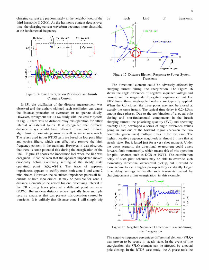
Figure 15. Distance Element Response to Power System
Transients
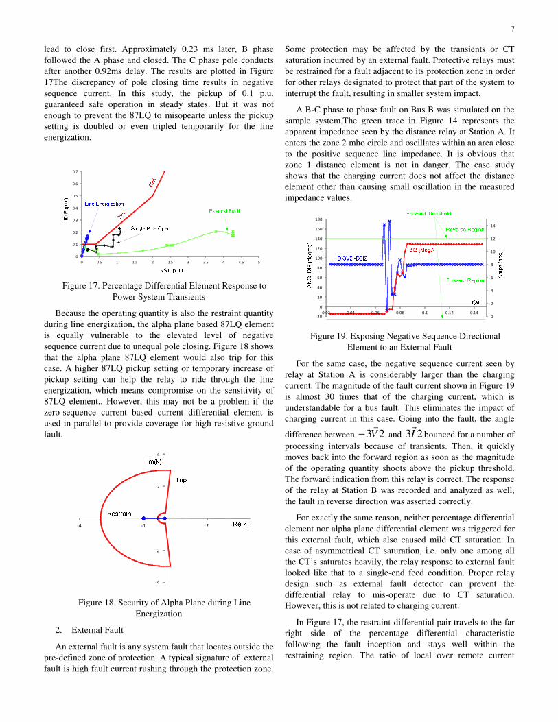
The directional element could be adversely affected by
charging current during line energization. The Figure 16
shows the angle difference of negative sequence voltage and
current, and the magnitude of negative sequence current. For
EHV lines, three single-pole breakers are typically applied.
When the CB closes, the three poles may not be closed at
exactly the same instant. The typical time delay is 0.2~1.5ms
among three phases. Due to the combination of unequal pole
closing and non-fundamental components in the inrush
charging current, the polarizing quantity (3V2) and operating
quantity (3I2) developed a series of angle difference values
going in and out of the forward region (between the two
horizontal green lines) multiple times in the test case. The
highest negative sequence magnitude is almost 3 times that at
steady state. But it lasted just for a very shot moment. Under
the worst scenario, the directional overcurrent could assert
forward fault momentarily, which means risk of mis-operation
for pilot schemes such as DCB or POTT. The coordination
delay of such pilot schemes may be able to override such
momentary directional overcurrent pickup, but it would be
more secure to use a higher pickup setting or slightly longer
time delay settings to handle such transients caused by
charging current at line energization in this example.
0
0.1
0.2
0.3
0.4
0.5
0.6
0.7
0.8
0.9
1
-180
-130
-80
-30
20
70
120
170
0.02 0.04 0.06 0.08 0.1 0.12 0.14
Figure 16. Negative Sequence Directional Element during
Line Energization
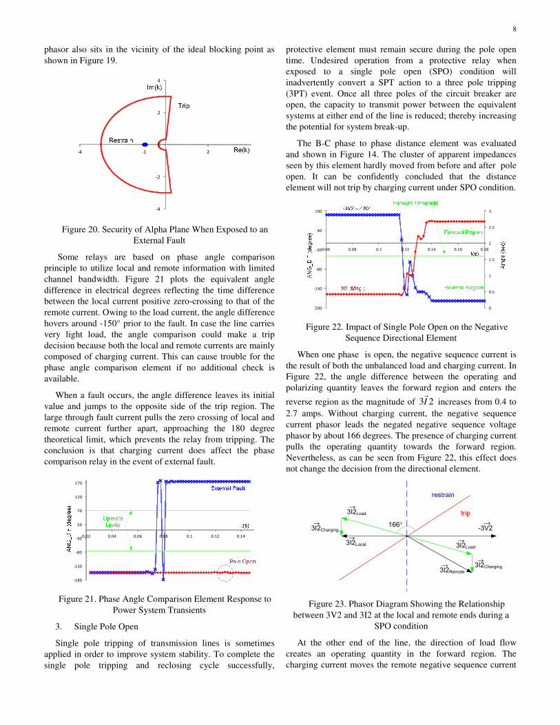
The negative sequence percentage differential element (87LQ)
was proven to be secure in steady state. In the event of line
energization, the 87LQ element can be affected by unequal
pole closing. In the RTDS case study, the A phase took the
7
lead to close first. Approximately 0.23 ms later, B phase
followed the A phase and closed. The C phase pole conducts
after another 0.92ms delay. The results are plotted in Figure
17The discrepancy of pole closing time results in negative
sequence current. In this study, the pickup of 0.1 p.u.
guaranteed safe operation in steady states. But it was not
enough to prevent the 87LQ to misopearte unless the pickup
setting is doubled or even tripled temporarily for the line
energization.
0
0.1
0.2
0.3
0.4
0.5
0.6
0.7
0 0.5 1 1.5 2 2.5 3 3.5 4 4.5 5
Figure 17. Percentage Differential Element Response to
Power System Transients
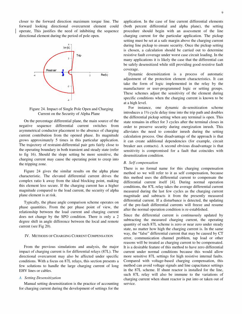
Because the operating quantity is also the restraint quantity
during line energization, the alpha plane based 87LQ element
is equally vulnerable to the elevated level of negative
sequence current due to unequal pole closing. Figure 18 shows
that the alpha plane 87LQ element would also trip for this
case. A higher 87LQ pickup setting or temporary increase of
pickup setting can help the relay to ride through the line
energization, which means compromise on the sensitivity of
87LQ element.. However, this may not be a problem if the
zero-sequence current based current differential element is
used in parallel to provide coverage for high resistive ground
fault.
-4
-2
0
2
4
-4 -1 2
Figure 18. Security of Alpha Plane during Line
Energization
2. External Fault
An external fault is any system fault that locates outside the
pre-defined zone of protection. A typical signature of external
fault is high fault current rushing through the protection zone.
Some protection may be affected by the transients or CT
saturation incurred by an external fault. Protective relays must
be restrained for a fault adjacent to its protection zone in order
for other relays designated to protect that part of the system to
interrupt the fault, resulting in smaller system impact.
A B-C phase to phase fault on Bus B was simulated on the
sample system.The green trace in Figure 14 represents the
apparent impedance seen by the distance relay at Station A. It
enters the zone 2 mho circle and oscillates within an area close
to the positive sequence line impedance. It is obvious that
zone 1 distance element is not in danger. The case study
shows that the charging current does not affect the distance
element other than causing small oscillation in the measured
impedance values.
0
2
4
6
8
10
12
14
-20
0
20
40
60
80
100
120
140
160
180
0.02 0.04 0.06 0.08 0.1 0.12 0.14
Figure 19. Exposing Negative Sequence Directional
Element to an External Fault
For the same case, the negative sequence current seen by
relay at Station A is considerably larger than the charging
current. The magnitude of the fault current shown in Figure 19
is almost 30 times that of the charging current, which is
understandable for a bus fault. This eliminates the impact of
charging current in this case. Going into the fault, the angle
difference between 23Vr
− and 23I
rbounced for a number of
processing intervals because of transients. Then, it quickly
moves back into the forward region as soon as the magnitude
of the operating quantity shoots above the pickup threshold.
The forward indication from this relay is correct. The response
of the relay at Station B was recorded and analyzed as well,
the fault in reverse direction was asserted correctly.
For exactly the same reason, neither percentage differential
element nor alpha plane differential element was triggered for
this external fault, which also caused mild CT saturation. In
case of asymmetrical CT saturation, i.e. only one among all
the CT’s saturates heavily, the relay response to external fault
looked like that to a single-end feed condition. Proper relay
design such as external fault detector can prevent the
differential relay to mis-operate due to CT saturation.
However, this is not related to charging current.
In Figure 17, the restraint-differential pair travels to the far
right side of the percentage differential characteristic
following the fault inception and stays well within the
restraining region. The ratio of local over remote current
8
phasor also sits in the vicinity of the ideal blocking point as
shown in Figure 19.
-4
-2
0
2
4
-4 -1 2
Figure 20. Security of Alpha Plane When Exposed to an
External Fault
Some relays are based on phase angle comparison
principle to utilize local and remote information with limited
channel bandwidth. Figure 21 plots the equivalent angle
difference in electrical degrees reflecting the time difference
between the local current positive zero-crossing to that of the
remote current. Owing to the load current, the angle difference
hovers around -150° prior to the fault. In case the line carries
very light load, the angle comparison could make a trip
decision because both the local and remote currents are mainly
composed of charging current. This can cause trouble for the
phase angle comparison element if no additional check is
available.
When a fault occurs, the angle difference leaves its initial
value and jumps to the opposite side of the trip region. The
large through fault current pulls the zero crossing of local and
remote current further apart, approaching the 180 degree
theoretical limit, which prevents the relay from tripping. The
conclusion is that charging current does affect the phase
comparison relay in the event of external fault.
-180
-130
-80
-30
20
70
120
170
0.02 0.04 0.06 0.08 0.1 0.12 0.14
Figure 21. Phase Angle Comparison Element Response to
Power System Transients
3. Single Pole Open
Single pole tripping of transmission lines is sometimes
applied in order to improve system stability. To complete the
single pole tripping and reclosing cycle successfully,
protective element must remain secure during the pole open
time. Undesired operation from a protective relay when
exposed to a single pole open (SPO) condition will
inadvertently convert a SPT action to a three pole tripping
(3PT) event. Once all three poles of the circuit breaker are
open, the capacity to transmit power between the equivalent
systems at either end of the line is reduced; thereby increasing
the potential for system break-up.
The B-C phase to phase distance element was evaluated
and shown in Figure 14. The cluster of apparent impedances
seen by this element hardly moved from before and after pole
open. It can be confidently concluded that the distance
element will not trip by charging current under SPO condition.
0
0.5
1
1.5
2
2.5
3
-200
-140
-80
-20
40
100
0.06 0.08 0.1 0.12 0.14 0.16 0.18
Figure 22. Impact of Single Pole Open on the Negative
Sequence Directional Element
When one phase is open, the negative sequence current is
the result of both the unbalanced load and charging current. In
Figure 22, the angle difference between the operating and
polarizing quantity leaves the forward region and enters the
reverse region as the magnitude of 23Ir
increases from 0.4 to
2.7 amps. Without charging current, the negative sequence
current phasor leads the negated negative sequence voltage
phasor by about 166 degrees. The presence of charging current
pulls the operating quantity towards the forward region.
Nevertheless, as can be seen from Figure 22, this effect does
not change the decision from the directional element.
-3V2
3I2Load
3I2Charging
3I2Load
3I2Charging
3I2Local
3I2Remote
166°
restrain
trip
Figure 23. Phasor Diagram Showing the Relationship
between 3V2 and 3I2 at the local and remote ends during a
SPO condition
At the other end of the line, the direction of load flow
creates an operating quantity in the forward region. The
charging current moves the remote negative sequence current
9
closer to the forward direction maximum torque line. The
forward looking directional overcurrent element could
operate. This justifies the need of inhibiting the sequence
directional element during the period of pole open.
-4
-2
0
2
4
-4 -1 2
Figure 24. Impact of Single Pole Open and Charging
Current on the Security of Alpha Plane
On the percentage differential plane, the main source of the
negative sequence differential current switches from
asymmetrical conductor placement to the absence of charging
current contribution from the opened phase. Its magnitude
grows approximately 5 times in this particular application.
The trajectory of restraint-differential pair gets fairly close to
the operating boundary in both transient and steady state (refer
to fig 16). Should the slope setting be more sensitive, the
charging current may cause the operating point to creep into
the tripping zone.
Figure 24 gives the similar results on the alpha plane
characteristic. The elevated differential current drives the
complex ratio k away from the ideal blocking point, making
this element less secure. If the charging current has a higher
magnitude compared to the load current, the security of alpha
plane element is at risk.
Typically, the phase angle comparison scheme operates on
phase quantities. From the per phase point of view, the
relationship between the load current and charging current
does not change by the SPO condition. There is only a 2
degree shift in angle difference between the local and remote
current (see Fig 20).
IV. METHODS OF CHARGING CURRENT COMPENSATION
From the previous simulations and analysis, the major
impact of charging current is for differential relays (87L). The
directional overcurrent may also be affected under specific
conditions. With a focus on 87L relays, this section presents a
few solutions to handle the large charging current of long
EHV lines or cables.
A. Setting Desensitization
Manual setting desensitization is the practice of accounting
for charging current during the development of settings for the
application. In the case of line current differential elements
(both percent differential and alpha plane), the setting
procedure should begin with an assessment of the line
charging current for the particular application. The pickup
setting must be set at a safe margin above the charging current
during line pickup to ensure security. Once the pickup setting
is chosen, a calculation should be carried out to determine
resistive fault coverage under worst case circuit loading. In the
many applications it is likely the case that the differential can
be safely desensitized while still providing good resistive fault
coverage.
Dynamic desensitization is a process of automatic
adjustment of the protection element characteristics. It can
take the form of logic implemented in the relay by the
manufacturer or user-programmed logic or setting groups.
These schemes adjust the sensitivity of the element during
specific conditions when the charging current is known to be
at a high level.
For instance, one dynamic de-sensitization scheme
introduces a 1½ cycle delay time into the trip path and doubles
the differential pickup setting when any terminal is open. This
state remains in effect for 3 cycles after the terminal closes in
order to preserve security during energization inrush. This
alleviates the need to consider inrush during the setting
calculation process. One disadvantage of the approach is that
it can create additional dependencies (for example, circuit
breaker aux contacts). A second obvious disadvantage is that
sensitivity is compromised for a fault that coincides with
desensitization condition.
B. Self compensation
There is no formal name for this charging compensation
method so we will refer to it as self compensation, because
this method uses the differential current to compensate the
differential current itself [4]. During normal operation
conditions, the 87L relay takes the average differential current
measured during the last few cycles as the charging current
magnitude and subtracts it from the presently measured
differential current. If a disturbance is detected, the updating
of the pre-fault differential currents will freeze and resume
after the normal operation condition is re-established.
Since the differential current is continuously updated by
subtracting the measured charging current, the operating
quantity of such 87L scheme is zero or near zero under steady
state, no matter how high the charging current is. In the same
way, the “false” differential current that may be caused by CT
error, communication channel problem, tap load or other
reasons will be treated as charging current to be compensated.
It is a desirable feature of this method to have zero differential
current under normal conditions because this would allow
more sensitive 87L settings for high resistive internal faults.
Compared with voltage-based charging compensation, this
method can avoid voltage signals and line capacitance settings
in the 87L scheme. If shunt reactor is installed for the line,
such 87L relay will also be immune to the variations of
charging current when shunt reactor is put into or taken out of
service.
10
On one hand, this compensation method helps to increase the
87L sensitivity. On the other hand, it may introduce extra
differential current under external fault condition. For an
external fault, the voltage will be suppressed and the actual
charging current will be less than that at pre-fault condition.
Since the pre-fault differential current is taken as charging
current, the compensation process will result in “false”
differential current. The increased restraint currents or external
fault detector could help to prevent the 87L operation. But it
will be prudent to evaluate the 87L characteristic settings for
some EHV lines/cables or tap load applications.
Another concern of this compensation method is during the
line or cable energization process, the method cannot provide
any charging compensation simply because there is no current
prior to energization. From Figure 14, the transient current
caused by line capacitance could be quite high during
energization so the relay using this method may mis-operate if
the 87L were set for sensitivity. A possible solution is to
increase the 87L settings temporarily before and during the
energization. But it will compromise the line protection during
the energization process.
C. Voltage-based compensation
The modern line differential relay usually incorporates
voltage measurement for back up protections. When the
voltage signal is available, the instantaneous charging current
drawn by the line or cable can be calculated in real time by
applying equation (2) from Section II. The calculated charging
current is then subtracted from the operating quantity such that
the 87L relay can have greater sensitivity. The basis of
equation (2) is that the transmission line can be modeled as a
two port component shown in Figure 25. This representation
is called the transmission line T model. A more accurate way
of approximating a physical line is to use the PI model, where
the line capacitance is split evenly at the two line terminals.
Figure 25. Transmission Line T Model
Conversely, line current differential is no longer a current
only scheme if the voltage signal is involved in improving its
performance. In case of LOP conditions, the voltage input
from that phase is lost and so is the ability to carry out
charging current compensation at that terminal. An
enhancement employs the PI model method, which means
each of the two line terminals will apply half of the total line
capacitance in its charging current calculation. Under normal
conditions, both terminals contribute to charging current
compensation. If one terminal fails for any reason, the
remaining healthy terminal takes up the responsibility to
compensate for all the charging current. In addition to
providing redundancy, including the voltages from both line
ends in the algorithm also produces a more accurate result for
compensation.
dtVV
dCdt
dVC
dt
dVCI RS
LRLSL
ch /222
+⋅=⋅+⋅= (11)
From equation (11), the charging current is estimated based
on the averaged line voltage. This approach works wellwhen
the voltage profile of the line is not flat.
In addition to loss of potential (LOP), the location of
potential transformer (PT) affects the availability of
compensation as well. Assuming that the PT is placed on the
bus side of the CB, the charging current compensation needs
to be suspended if one phase of the CB is open. This is
because the bus voltage does not follow the change in line
voltage under SPO conditions. If it is still used to calculate the
line charging current, the 87L can be inaccurate in a SPT
application.
Tap
Point
Terminal X
Terminal Z
Terminal Y
87L
Relay X
87L
Relay Y
87L
Relay Z
87L Channel(Slave)
(Slave)
(Master)
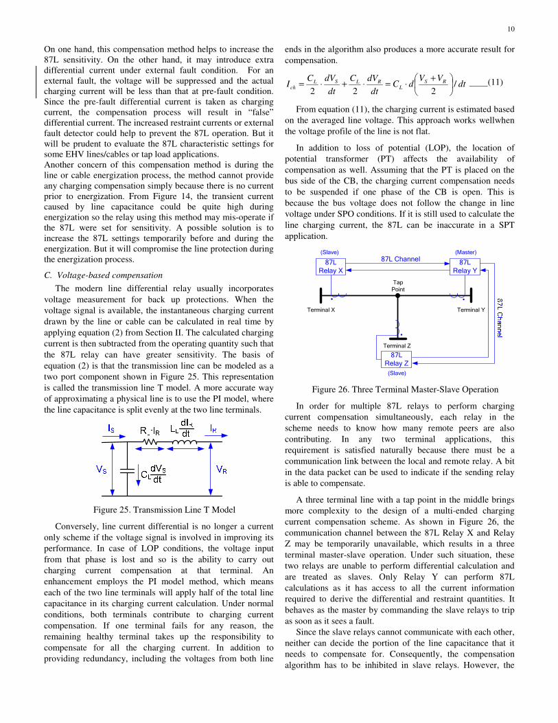
Figure 26. Three Terminal Master-Slave Operation
In order for multiple 87L relays to perform charging
current compensation simultaneously, each relay in the
scheme needs to know how many remote peers are also
contributing. In any two terminal applications, this
requirement is satisfied naturally because there must be a
communication link between the local and remote relay. A bit
in the data packet can be used to indicate if the sending relay
is able to compensate.
A three terminal line with a tap point in the middle brings
more complexity to the design of a multi-ended charging
current compensation scheme. As shown in Figure 26, the
communication channel between the 87L Relay X and Relay
Z may be temporarily unavailable, which results in a three
terminal master-slave operation. Under such situation, these
two relays are unable to perform differential calculation and
are treated as slaves. Only Relay Y can perform 87L
calculations as it has access to all the current information
required to derive the differential and restraint quantities. It
behaves as the master by commanding the slave relays to trip
as soon as it sees a fault.
Since the slave relays cannot communicate with each other,
neither can decide the portion of the line capacitance that it
needs to compensate for. Consequently, the compensation
algorithm has to be inhibited in slave relays. However, the
11
master relay is capable of handling all of the charging current
compensation for the 87L zone, albeit with reduced accuracy.
D. Other compensation methods
From literature [5, 6], the charging current may be handled by
unconventional current differential schemes. In [5], the 87L
relaying is built upon the calculated currents from a
distributed line parameter model and the charging current will
be eliminated in the calculated currents.
Figure 27. Voltages and currents of a UHV line
For a uniformly distributed line shown in Fig. 26, it is well
known that the voltage and current distributed along the line
have the following relationship.
t
ilir
x
u
∂
∂+=
∂
∂− 00 (12)
t
ucig
x
i
∂
∂+=
∂
∂− 00 (13)
Where 0r , 0l , 0g , 0c are series resistance, series inductance,
shunt conductance and shunt capacitance in unit length.
From (12) and (13), the positive sequence, negative sequence
or zero sequence currents at any point k on the line can be
calculated by
)()( ##
#### mk
c
mmkmmk lsh
Z
UlchII γγ −= (14)
)()( ##
#### nk
c
nnknnk lsh
Z
UlchII γγ −= (15)
where sh( ) and ch( ) are hyperbolic functions, Zc is the line
characteristic impedance, γ is the propagation constant and
xyl is the distance from point x to point y on the line. The # in
Eq. (14) and (15) are to be replaced by 1, 2 or 0 for positive,
negative or zero sequence currents. With sequence
components, the three phase currents at point k can be
obtained as well. Using positive sequence currents as example,
the differential current and restraint current of the 87L scheme
are based on the calculated currents at a specific point k on the
line,
111_ nkmkdiff III += (16)
111int_ nkmkrestra III −= (17)
Since the 87L operating and restraint quantities are derived
from the distributed line model per Eq. (12) ~ (15), the
charging current is excluded naturally. As with the
conventional voltage-based compensation, this method also
needs a voltage signal, but this method can take any point on
the line to perform differential and restraint calculation, which
can improve the sensitivity of 87L scheme, according to [5].
From the simulation tests in [5], the proposed 87L relay can
handle high resistive faults and is secure for external faults.
There are also recommendations in [5] on how to select the k
point to optimize the sensitivity and dependability of the 87L
relay. Similarly, there are other 87L schemes that use calculated
current per line modeling to eliminate the impact of charging
current for UHV lines. Theoretically, such 87L schemes can
provide alternative solutions to handle large charging current
for UHV lines or cables. But the practical applications and
operational experience of such 87L relays not evident at this
time.
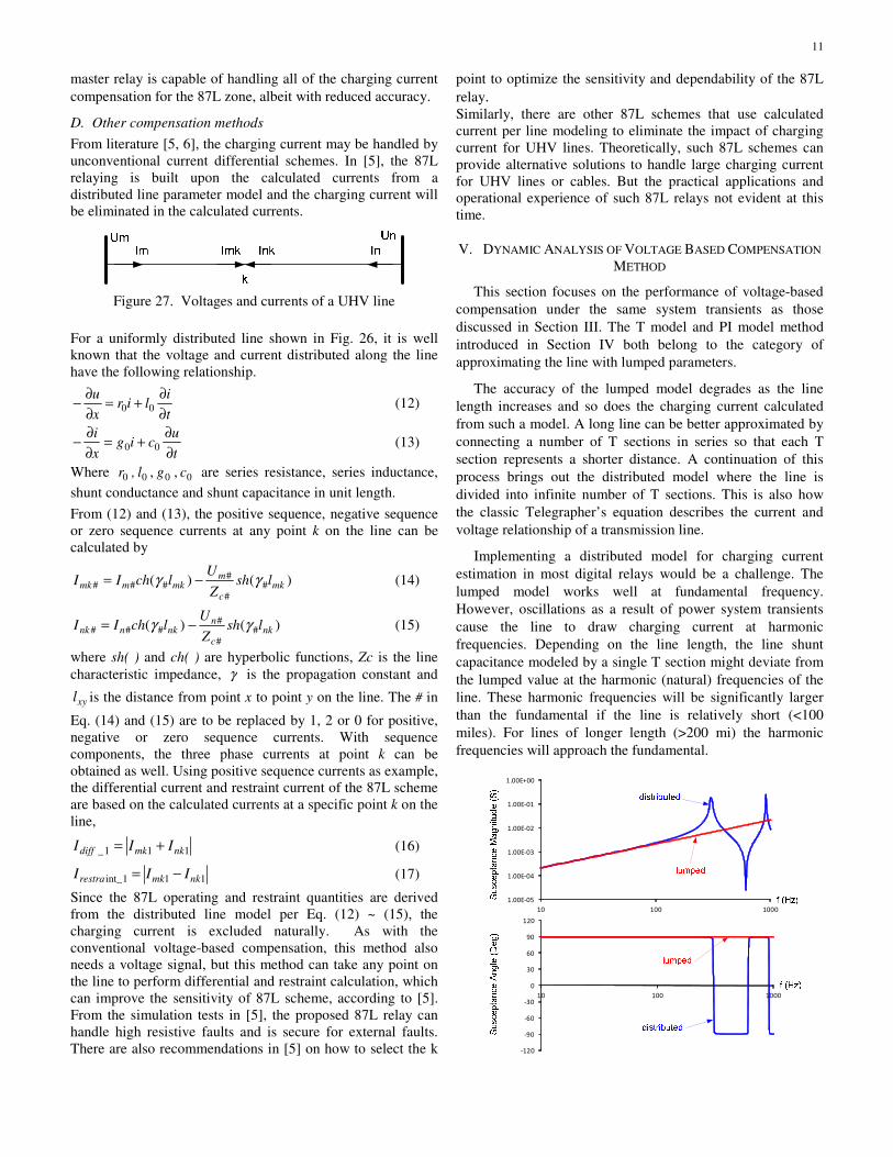
V. DYNAMIC ANALYSIS OF VOLTAGE BASED COMPENSATION
METHOD
This section focuses on the performance of voltage-based
compensation under the same system transients as those
discussed in Section III. The T model and PI model method
introduced in Section IV both belong to the category of
approximating the line with lumped parameters.
The accuracy of the lumped model degrades as the line
length increases and so does the charging current calculated
from such a model. A long line can be better approximated by
connecting a number of T sections in series so that each T
section represents a shorter distance. A continuation of this
process brings out the distributed model where the line is
divided into infinite number of T sections. This is also how
the classic Telegrapher’s equation describes the current and
voltage relationship of a transmission line.
Implementing a distributed model for charging current
estimation in most digital relays would be a challenge. The
lumped model works well at fundamental frequency.
However, oscillations as a result of power system transients
cause the line to draw charging current at harmonic
frequencies. Depending on the line length, the line shunt
capacitance modeled by a single T section might deviate from
the lumped value at the harmonic (natural) frequencies of the
line. These harmonic frequencies will be significantly larger
than the fundamental if the line is relatively short (<100
miles). For lines of longer length (>200 mi) the harmonic
frequencies will approach the fundamental.
-120
-90
-60
-30
0
30
60
90
120
10 100 1000
1.00E-05
1.00E-04
1.00E-03
1.00E-02
1.00E-01
1.00E+00
10 100 1000
12
Figure 28. Comparing the lumped and distributed line
capacitance model
Using the 765kV line data from the appendix, the
magnitude and angle of the shunt susceptance are plotted in
Figure 28. According to the lumped model, the line
susceptance has a magnitude proportional to the system
frequency and its angle is always at 90 degrees. The
distributed model offers an accurate representation until the
system frequency goes above 120Hz. As the frequency ramps
up, the susceptance magnitude given by the distributed model
is either higher or lower than that given by the lumped model,
which is a straight line with a constant slope. In addition, the
overall characteristic of line shunt component shifts from
being capacitive to being reactive at certain frequencies.
The theoretical analysis can be verified by the simulation
results presented below. These three transients have one thing
in common, i.e. a temporary harmonic surge in the first a few
cycles of the event.
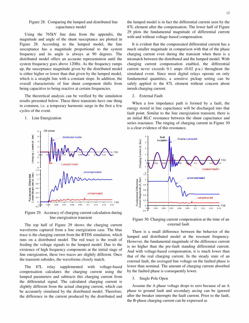
1. Line Energization
-0.2
0
0.2
0.4
0.6
0.8
1
1.2
1.4
0.04 0.05 0.06 0.07 0.08 0.09 0.1 0.11 0.12 0.13
-6
-4
-2
0
2
4
6
8
0.04 0.05 0.06 0.07 0.08 0.09 0.1 0.11 0.12 0.13
t (s)
Lumped model
distributed model
compensated
uncompensated
t (s)
CB closes
Figure 29. Accuracy of charging current calculation during
line energization transient
The top half of Figure 29 shows the charging current
waveforms captured from a line energization case. The blue
trace is the charging current from the RTDS simulation, which
runs on a distributed model. The red trace is the result of
feeding the voltage signals to the lumped model. Due to the
existence of high frequency components at the initial stage of
line energization, these two traces are slightly different. Once
the transient subsides, the waveforms closely match.
The 87L relay supplemented with voltage-based
compensation calculates the charging current using the
lumped parameters and subtracts this charging current from
the differential signal. The calculated charging current is
slightly different from the actual charging current, which can
be accurately simulated by the distributed model. Therefore,
the difference in the current produced by the distributed and
the lumped model is in fact the differential current seen by the
87L element after the compensation. The lower half of Figure
29 plots the fundamental magnitude of differential current
with and without voltage-based compensation.
It is evident that the compensated differential current has a
much smaller magnitude in comparison with that of the phase
charging current even during the transient when there is a
mismatch between the distributed and the lumped model. With
charging current compensation enabled, the differential
current never exceeds 0.1 amps (0.02 p.u.) throughout the
simulated event. Since most digital relays operate on only
fundamental quantities, a sensitive pickup setting can be
safely applied to the 87L element without concern about
inrush charging current.
2. External Fault
When a low impedance path is formed by a fault, the
energy stored in line capacitance will be discharged into that
fault point. Similar to the line energization transient, there is
an initial RLC resonance between the shunt capacitance and
series reactance. The ringing of charging current in Figure 30
is a clear evidence of this resonance.
-0.2
0
0.2
0.4
0.6
0.8
1
1.2
0.04 0.05 0.06 0.07 0.08 0.09 0.1 0.11 0.12 0.13
-2
-1
0
1
2
3
4
0.04 0.05 0.06 0.07 0.08 0.09 0.1 0.11 0.12 0.13
Charging Current (A, Sec)
Fundamental Differential
Current Magnitude (A, Sec)
Figure 30. Charging current compensation at the time of an
external fault
There is a small difference between the behavior of the
lumped and distributed model at the resonant frequency.
However, the fundamental magnitude of the difference current
is no higher than the pre-fault standing differential current.
And with voltage-based compensation, it is much lower than
that of the real charging current. In the steady state of an
external fault, the averaged line voltage on the faulted phase is
lower than nominal. The amount of charging current absorbed
by the faulted phase is consequently lower.
3. Single Pole Open
Assume the A phase voltage drops to zero because of an A
phase to ground fault and secondary arcing can be ignored
after the breaker interrupts the fault current. Prior to the fault,
the B-phase charging current can be expressed as
13
BCBCBAABBGBGBch VCjVCjVCjI ⋅+⋅+⋅= ωωω (18)
During the pole open interval, BAV is identical to
BGV
considering that the faulty phase is grounded. This effect is
visualized in Figure 31.
Figure 31. Shift of charging current phasor due to SPO
SPOBcI _
represents the charging current phasor at the time
when the breaker A phase is open. It has a slightly smaller
magnitude and advanced angle compared with BcI .
-0.2
0
0.2
0.4
0.6
0.8
1
0.09 0.11 0.13 0.15 0.17
-2
-1.5
-1
-0.5
0
0.5
1
1.5
0.09 0.11 0.13 0.15 0.17
Charging Current (A, Sec)
Fundamental Differential
Current Magnitude (A, Sec)
Figure 32. Impact of SPO on line charging current
From Figure 32, it can be observed that the high frequency
discharge transient on the faulted phase lasted for about two
cycles. The transition of B-phase and C-phase charging
currents from their pre-fault values to their respective pole
open state values completed within the same time frame. The
top oscillography in Figure 32 proves the anticipated
magnitude reduction and phase shift. The compensated
differential current magnitude plotted in the lower half of
Figure 32 dropped to 0.05A once the transient came to an end.
To conclude, the 87L element will not be stressed by any
above events as long as the voltage based charging current
compensation is active.
VI. APPLICATION GUIDELINES
Section II showed that charging current is mainly a concern
for line current differential and phase comparison schemes.
Indeed, these are the only types of relay for which
manufacturers provide charging current compensation. In
addition, sequence directional elements should be checked for
line energization and open pole operation. In this section we
provide guidelines for determining when to use charging
current compensation for current differential applications.
Step 1 in the process is determination of the charging
current. Shunt capacitances can be calculated using (6) and (7)
or using a line constants program. The difference between the
results obtained by the two approaches is typically less than
10%. Charging current is then calculated using (8).
When charging current is significant, sequence directional
elements could misoperate during line energization. In this
case consider either to de-sensitize the element or to delay
operation when the line is energized. Sequence directional
elements should be blocked by open-pole logic on lines that
employ single pole tripping.
The pickup setting of the phase differential element must
be set higher than the value of the standing charging current.
To ensure security during line energization a margin of 200%
could be considered. In relays which employ dynamic
desensitization, a lower margin (150%) can be chosen;
depending on the particular implementation.
Step 2 checks the coverage provided for resistive faults
during line loading. In general the following equation gives
the internal ground fault current for a two terminal line [8].
( )[ ]( ) ( ) F
LOADPHNPHG
RCLZdSZCLZdSZ
LZdSZIVIf
⋅+⋅⋅++⋅⋅+
⋅+⋅−⋅=
30001112
113
(19)
Where
RZLZSZ
LZdRZC
RZLZSZ
LZdRZC
000
0)1(00,
111
1)1(11
++
⋅−+=
++
⋅−+=
(20)
Where Z1R, Z0R, Z1S, and Z0S are the positive and zero
sequence source impedances, Z1L and Z0L are the positive
and zero sequence line impedances. VPHN is the line to neutral
voltage, d is the location of the fault (0-1) and RF is the fault
resistance.
The fault current should be checked for d=0 and d=1 for
the highest fault resistance for which the phase elements need
to operate. This value should be greater than the pickup setting
chosen in step 1.
For an alpha plane element the ratio K can be calculated as
( ) ( )
PHG
LOAD
PHG
LOAD
PH
If
ICC
If
ICC
K
⋅−+⋅
⋅+−+−⋅
=
3012
301112
(21)
Adequate coverage is verified by checking the magnitude
and angle of KPH against the ratio and blocking angle settings
of the element.
For a percent differential the restraint signal is
LOADPHG
R IIf
I +≈2
(22)
Adequate coverage is verified by checking that the
differential current is greater than the IR multiplied by the
slope setting.
Sequence differential elements applied on lines employing
single pole tripping and with significant charging current
should either be de-sensitized or be blocked by open pole
logic.
14
If the differential element cannot provide the needed fault
coverage then the use of line charging compensation is
warranted. Relays which employ voltage-based compensation
require that the positive and zero sequence capacitance (or
susceptance) of the line be entered as a setting. Consequently,
the differential elements can now be set without having to
consider charging current. However, since a voltage
measurement is required, voltage-based compensation is
impacted by loss of potential or fuse-failure events. Some
relays have a built-in logic which allows the user to fallback to
more secure settings under LOP conditions. Other relays may
not have built-in logic but the same functionality may be
achievable using programmable logic and setting groups. In
either case such schemes improve the availability of the
differential protection but require additional effort in settings
development. Relays which employ the self-compensation
method described in section IV benefit from reduced settings
requirements.
When negative sequence and zero sequence elements are
applied an alternate strategy is to require the phase elements
only to be sensitive for three-phase faults. The fault resistance
requirements are lower for this fault type. As a result more
margin is available for setting the element. The sequence
elements provide excellent resistive fault coverage irrespective
of loading. Sequence charging currents are significantly lower,
even on un-transposed lines as evidenced in section II. The
relaxed sensitivity requirement on the phase element lessens
the need for charging current compensation.
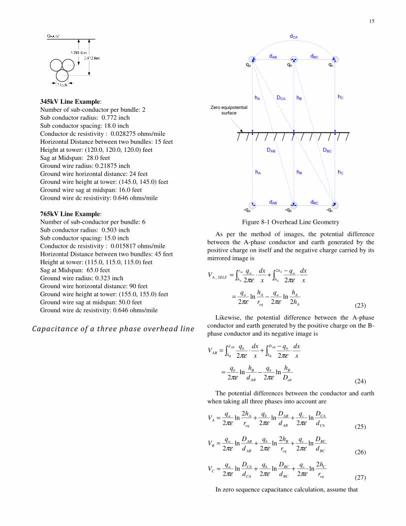
Shunt reactors are often applied on long lines for voltage
control (figure 32). These reactors will provide a portion of
the charging current. This will create an error in compensation
provided by voltage-based schemes. One solution to the
problem is to calculate the combined susceptance of the
parallel inductive and capacitive branches and to use this
value when setting the relay. However, there are several
problems with this approach. The first problem is that the
degree to which the two branches cancel will differ in the
transient and steady states. As a consequence capacitive inrush
can still occur. The second problem is dealing with reactor
switching. To achieve optimal compensation different settings
would need to be applied with the reactors in and out of
service and this may be impractical because changes need to
be made to both local and remote relays.
Figure 32. Transmission line with shunt reactors
A better solution is to measure the contribution of the
reactors to the zone as shown in figure 33. Bringing the CT at
shunt reactor branch into the 87L scheme, the shunt reactor is
excluded from the 87L protection zone. Now the voltage
based compensation can use full susceptance of the line as its
setting once again. Reactor switching and line energization are
no longer an issue.
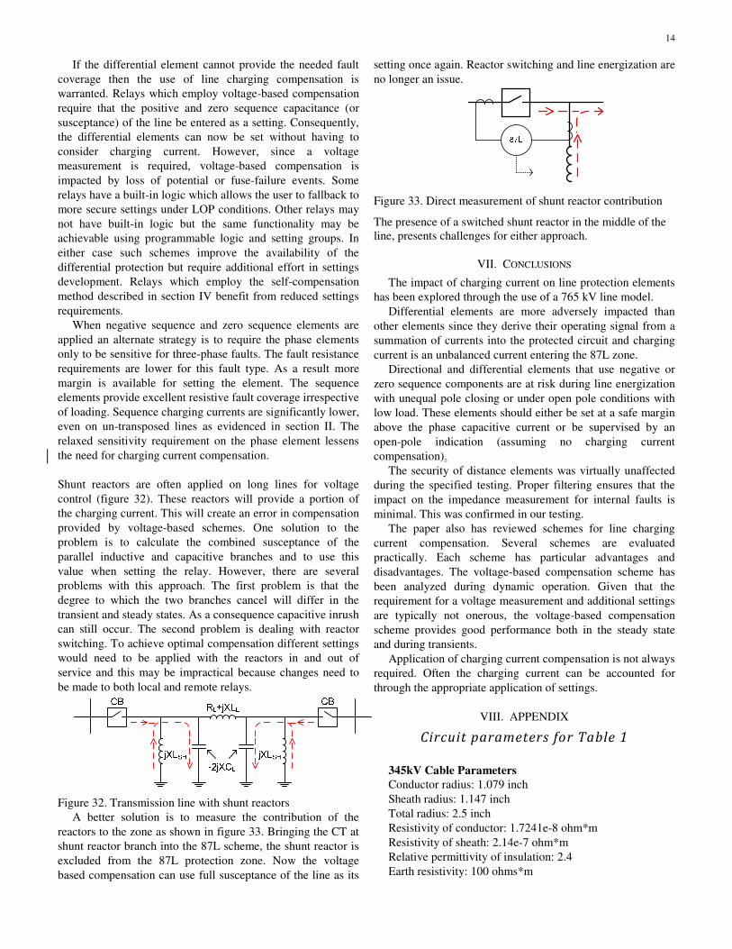
Figure 33. Direct measurement of shunt reactor contribution
The presence of a switched shunt reactor in the middle of the
line, presents challenges for either approach.
VII. CONCLUSIONS
The impact of charging current on line protection elements
has been explored through the use of a 765 kV line model.
Differential elements are more adversely impacted than
other elements since they derive their operating signal from a
summation of currents into the protected circuit and charging
current is an unbalanced current entering the 87L zone.
Directional and differential elements that use negative or
zero sequence components are at risk during line energization
with unequal pole closing or under open pole conditions with
low load. These elements should either be set at a safe margin
above the phase capacitive current or be supervised by an
open-pole indication (assuming no charging current
compensation).
The security of distance elements was virtually unaffected
during the specified testing. Proper filtering ensures that the
impact on the impedance measurement for internal faults is
minimal. This was confirmed in our testing.
The paper also has reviewed schemes for line charging
current compensation. Several schemes are evaluated
practically. Each scheme has particular advantages and
disadvantages. The voltage-based compensation scheme has
been analyzed during dynamic operation. Given that the
requirement for a voltage measurement and additional settings
are typically not onerous, the voltage-based compensation
scheme provides good performance both in the steady state
and during transients.
Application of charging current compensation is not always
required. Often the charging current can be accounted for
through the appropriate application of settings.
VIII. APPENDIX
Circuit parameters for Table 1
345kV Cable Parameters
Conductor radius: 1.079 inch
Sheath radius: 1.147 inch
Total radius: 2.5 inch
Resistivity of conductor: 1.7241e-8 ohm*m
Resistivity of sheath: 2.14e-7 ohm*m
Relative permittivity of insulation: 2.4
Earth resistivity: 100 ohms*m
15
345kV Line Example:
Number of sub-conductor per bundle: 2
Sub conductor radius: 0.772 inch
Sub conductor spacing: 18.0 inch
Conductor dc resistivity : 0.028275 ohms/mile
Horizontal Distance between two bundles: 15 feet
Height at tower: (120.0, 120.0, 120.0) feet
Sag at Midspan: 28.0 feet
Ground wire radius: 0.21875 inch
Ground wire horizontal distance: 24 feet
Ground wire height at tower: (145.0, 145.0) feet
Ground wire sag at midspan: 16.0 feet
Ground wire dc resistivity: 0.646 ohms/mile
765kV Line Example:
Number of sub-conductor per bundle: 6
Sub conductor radius: 0.503 inch
Sub conductor spacing: 15.0 inch
Conductor dc resistivity : 0.015817 ohms/mile
Horizontal Distance between two bundles: 45 feet
Height at tower: (115.0, 115.0, 115.0) feet
Sag at Midspan: 65.0 feet
Ground wire radius: 0.323 inch
Ground wire horizontal distance: 90 feet
Ground wire height at tower: (155.0, 155.0) feet
Ground wire sag at midspan: 50.0 feet
Ground wire dc resistivity: 0.646 ohms/mile
Capacitance of a three phase overhead line
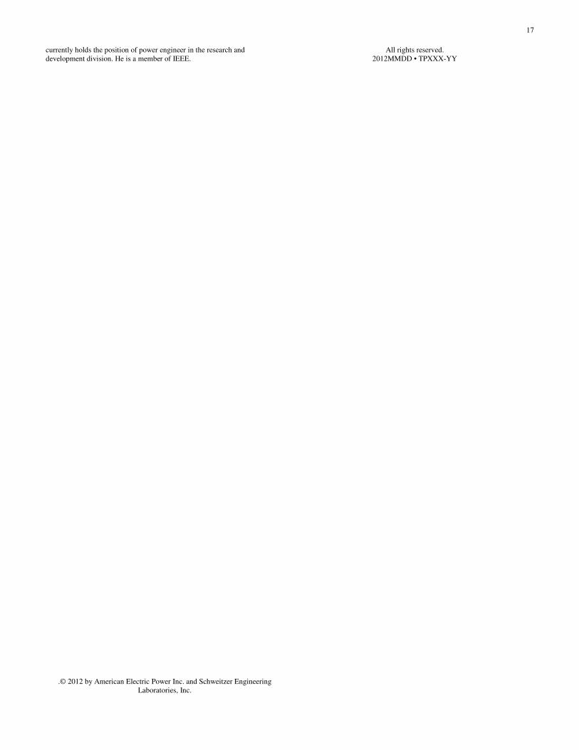
dAB dBC
hBhA hC
dCA
dAB dBC
Zero equipotential surface
hBhA hC
qbqa qc
-qb-qa -qc
DAB DBC
DCA
Figure 8-1 Overhead Line Geometry
As per the method of images, the potential difference
between the A-phase conductor and earth generated by the
positive charge on itself and the negative charge carried by its
mirrored image is
x
dxq
x
dxqV
A
A
eq
A
h
h
ar
h
aSELFA ⋅
−+⋅= ∫∫
2
_22 πεπε
A
Aa
eq
Aa
h
hq
r
hq
2ln
2ln
2 πεπε−=
(23)
Likewise, the potential difference between the A-phase
conductor and earth generated by the positive charge on the B-
phase conductor and its negative image is
x
dxq
x
dxqV
AB
B
AB
B
D
h
bd
h
bAB
⋅−
+⋅= ∫∫ πεπε 22
ab
Bb
AB
Bb
D
hq
d
hqln
2ln
2 πεπε−=
(24)
The potential differences between the conductor and earth
when taking all three phases into account are
CA
CAc
AB
ABb
eq
AaA
d
Dq
d
Dq
r
hqV ln
2ln
2
2ln
2 πεπεπε++=
(25)
BC
BCc
eq
Bb
AB
ABaB
d
Dq
r
hq
d
DqV ln
2
2ln
2ln
2 πεπεπε++=
(26)
eq
Cc
BC
BCb
CA
CAaC
r
hq
d
Dq
d
DqV
2ln
2ln
2ln
2 πεπεπε++=
(27)
In zero sequence capacitance calculation, assume that
16
0qqqq cba ===
(28)
cba VVVV ++=03
(29)
The result of adding equation (25), (26) and (27) together is
222
222
0
3
00 ln
2
222ln
23
CABCAB
CABCAB
eq
CBA
ddd
DDDq
r
hhhqV
⋅⋅
⋅⋅+
⋅⋅=
πεπε
( )6
6
0
3
3
0 ln2
2ln
2 m
m
eq
m
d
Dq
r
hq
πεπε+=
(30)
2
2
00
2ln
2 meq
mm
dr
DhqV
⋅
⋅=
πε (31)
The tower height (hm) is typically much larger the distance
between the phase conductors (dm). Therefore, Dm can be
approximated by 2hm and equation (31) can be rewritten as
( )2
3
00
2ln
2 meq
m
dr
hqV
⋅=
πε (32)
From (32), the zero sequence line capacitance is
( )2
3
0
00
2ln
2
meq
m
dr
hV
qC
⋅
==πε
(33)
When calculating the positive sequence capacitance, the
relationship turns into
cba qqq ⋅=⋅= 2αα
(34)
cba VVVV ⋅+⋅+= 2
13 αα
(35)
Substituting equations (25) through (27) for the phase
voltages in equation (35) yields
+⋅⋅
=31
222ln
23
eq
CBAa
r
hhhqV
πε
CABCAB
CABCABa
CABCAB
CABCABa
ddd
DDDq
ddd
DDDq
⋅⋅
⋅⋅⋅+
⋅⋅
⋅⋅⋅ln
2ln
2
2
πε
α
πε
α
( ) ( )3
32
3
3
ln2
2ln
2 m
ma
eq
ma
d
Dq
r
hq
πε
αα
πε
⋅++=
( )33
332
ln2 meq
mma
Dr
dhq
⋅
⋅=
πε (36)
Since Dm ≈ 2hm, the above equation can be simplified to
3
3
1 ln2
3eq
ma
r
dqV
πε=
(37)
The positive sequence line capacitance can thus be found
as
eq
m
r
dC
ln
21
πε=
(38)
IX. REFERENCES
[1] B. Kasztenny, I. Voloh, E. Udren, “Rebirth of the Phase
Comparison Line Protection Principle”, ???
[2] W. Stevenson, J. Grainger, "Power System Analysis,
1994
[3] T. Kase, Y. Kurosawa, "Charging Current Compensation
for Distance Protection", Power Engineering Society
General Meeting, vol. 3, pp. 2683-2688, June 2005
[4] Z. Gajic, I. Brncic, F.Rios, “Multi-terminal Line
Differential Protection with Innovative Charging Current
Compensation Algorithm”, 10th
IET Int. Conf. on Dev. in
Power Systems Protection, Mar. 29, 2010
[5] Z. Y. Xu, Z. Q. Du, Y.K. Wu, Q.X. Yang, and J.L. He, "A
current differential relay for a 1000kV UHV transmission
line," IEEE Trans. Power Del., vol. 22, no. 3, pp. 1392–
1399, Jul. 2007.
[6] Y. Qiao, C. Qing, "An Improved Current Differential
Protective Principle of UHV Transmission Line", 2011
Asia-Pacific Power and Energy Engineering Conference
(APPEEC), Mar. 2011
[7] B. Kasztenny, G. Benmouyal, H. J. Altuve, and N.
Fischer, “Tutorial on Operating Characteristics of
Microprocessor-Based Multiterminal Line Current
Differential Relays,” 38th Annual Western Protective
Relay Conference, Spokane, WA, October 18–20, 2011.
[8] G. Benmouyal “The Trajectories of Line Current
Differential Faults in the Alpha Plane”, ???
X. BIOGRAPHIES
Yiyan Xue received his B.Eng. from Zhejiang University in 1993 and M.Sc.
from the University of Guelph in 2007. He is currently a Senior Engineer in
AEP P&C Standards Group, working on protection standards, relay settings,
fault analysis and simulation studies. Before joining AEP, he was an
Application Engineer with GE Multilin to provide consulting services on relay
settings, scheme design and RTDS studies. Prior to GE, he had 10 years with
ABB Inc. working on P&C system design, commissioning of relays and RTU
systems. He is a senior member of IEEE and a Professional Engineer
registered in Ohio.
Dale Finney received a bachelor of engineering degree from Lakehead
University in 1988 and a Master of Engineering degree from the University of
Toronto in 2002. He began his career with Ontario Hydro, where he worked
as a protection and control engineer. Currently, Dale is employed as a senior
power engineer with Schweitzer Engineering Laboratories, Inc. His areas of
interest include generator protection, line protection, and substation
automation. Dale holds of several patents and has authored more than twenty
papers in the area of power system protection. He is a member of the main
committee of the IEEE PSRC, a member of the rotating machinery
subcommittee, and a registered professional engineer in the province of
Ontario.
Bin Le received his BSEE from Shanghai Jiao Tong University in 2006 and
an MSEE degree from the University of Texas at Austin in 2008. He has been
employed by Schweitzer Engineering Laboratories, Inc. ever since. Mr. Le
17
currently holds the position of power engineer in the research and
development division. He is a member of IEEE.
.© 2012 by American Electric Power Inc. and Schweitzer Engineering
Laboratories, Inc.
All rights reserved.
2012MMDD • TPXXX-YY
Recommended