Carrier and Timing Synchronization of
BPSK via LDPC Code Feedback
Esteban Vallés, Richard Weseland John Villasenor
Electrical Engineering DepartmentUniv. California, Los Angeles
Christopher Jones Marvin Simon
Jet Propulsion LaboratoryPasadena, CA
2
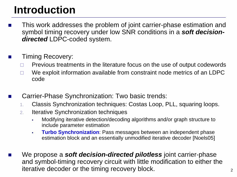
IntroductionThis work addresses the problem of joint carrier-phase estimation and symbol timing recovery under low SNR conditions in a soft decision-directed LDPC-coded system.
Timing Recovery:Previous treatments in the literature focus on the use of output codewordsWe exploit information available from constraint node metrics of an LDPC code
Carrier-Phase Synchronization: Two basic trends:1. Classis Synchronization techniques: Costas Loop, PLL, squaring loops.2. Iterative Synchronization techniques
Modifying iterative detection/decoding algorithms and/or graph structure to include parameter estimationTurbo Synchronization: Pass messages between an independent phase estimation block and an essentially unmodified iterative decoder [Noels05]
We propose a soft decision-directed pilotless joint carrier-phase and symbol-timing recovery circuit with little modification to either the iterative decoder or the timing recovery block.
3
Joint Estimation Algorithm
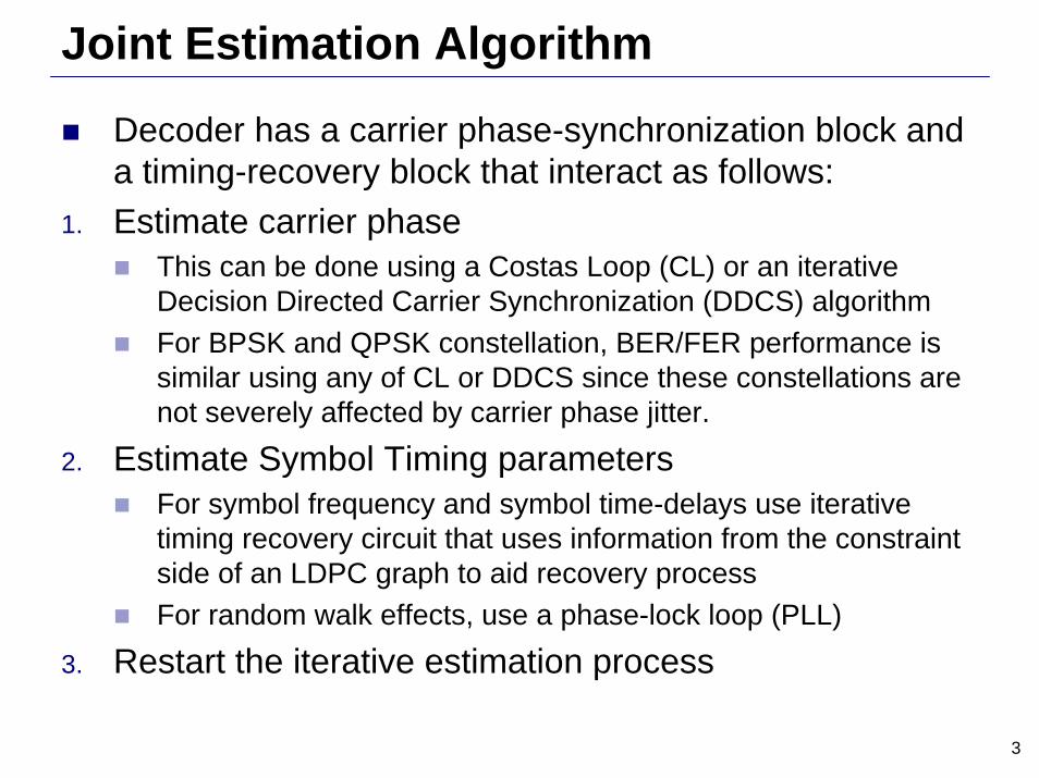
Decoder has a carrier phase-synchronization block and a timing-recovery block that interact as follows:
1. Estimate carrier phaseThis can be done using a Costas Loop (CL) or an iterative Decision Directed Carrier Synchronization (DDCS) algorithmFor BPSK and QPSK constellation, BER/FER performance is similar using any of CL or DDCS since these constellations are not severely affected by carrier phase jitter.
2. Estimate Symbol Timing parametersFor symbol frequency and symbol time-delays use iterative timing recovery circuit that uses information from the constraint side of an LDPC graph to aid recovery processFor random walk effects, use a phase-lock loop (PLL)
3. Restart the iterative estimation process
4
Transmission Model
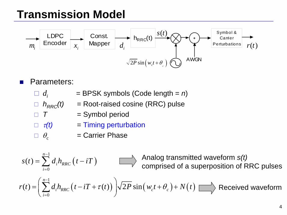
Parameters:di = BPSK symbols (Code length = n) hRRC(t) = Root-raised cosine (RRC) pulse T = Symbol periodτ(t) = Timing perturbationθc = Carrier Phase
Analog transmitted waveform s(t)comprised of a superposition of RRC pulses
( ) ( ) ( )1
0
( ) ( ) 2 sinn
i RRC c ci
r t d h t iT t P w t N tτ θ−
=
⎛ ⎞= − + + +⎜ ⎟⎝ ⎠∑ Received waveform
( )1
0( )
n
i RRCi
s t d h t iT−
=
= −∑
LDPCEncoder
im
AWGN
Const.Mapper
ixhRRC(t)
id+
Symbol &Carrier
Perturbations
( )2 sinccP w t θ+
( )r t
( )s t
5
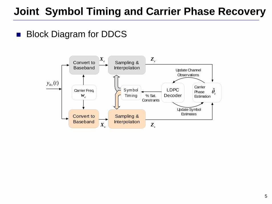
Joint Symbol Timing and Carrier Phase Recovery
Block Diagram for DDCS
Carrier Freq.% Sat.
Constrants
Update SymbolEstimates
Update ChannelObservations
( )Rxy t
cw
Sampling &Interpolation
cX
CarrierPhaseEstimation
cθ
Sampling &Interpolation
sX
cZ
sZ
LDPCDecoder
Sym bolTim ing
Convert toBaseband
Convert toBaseband
6
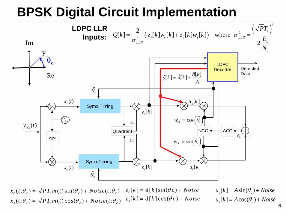
BPSK Digital Circuit Implementation
θc
y1
Re
Im
[ ] [ ] sin( )[ ] [ ] cos( )
c
s
z k d k c Noisez k d k c Noise
θθ
= +
= +[ ] sin( )[ ] cos( )
c c
s c
u k A Noiseu k A Noise
θθ
= +
= +( ; ) ( ) sin( ) ( ; )
( ; ) ( ) cos( ) ( ; )c c s c c
s c s c c
x t PT m t Noise t
x t PT m t Noise t
θ θ θ
θ θ θ
= +
= +
( )( )2
22
2[ ] [ ] [ ] [ ] [ ] where 2
s
s c c s LLRsLLR
o
PTQ k z k w k z k w k E
N
σσ
= + =
( )ˆcosck cw θ=
LDPC LLR Inputs:
DetectedData
Symb.Timing( )sx t
Symb.Timing( )cx t
LDPCDecoder
NCO ACC
( )ˆsinsk cw θ=
ˆ[ ]ˆˆ[ ] [ ] n ky k d kA
= +
[ ]sz k
[ ]cz k [ ]cu k
[ ]su k
keQuadrant
1±
1±
cθ
cθ
90°
( )Rxy t
7
Carrier Phase Recovery: MotivationWhen designing communication systems engineers need to decide whether or not to suppress the transmitted carrier power
Total power = Carrier Power + Data Power Pt=Pc+PdCarrier Power: related to the accuracy of the carrier synch processData Power: related to the accuracy of the data detection process (in the presence of perfect carrier synchronization).
System design requires a proper trade off between these power requirements to minimize the average error probability of the system.
Suppressed-carrier circuits: Costas loop
Require a larger SNR to track the carrier with a given accuracy.Phase estimation has jitter
Decision Directed Carrier Synchronization:Parameter estimation improves with the iteration processSquaring loss tends to unity as iterations increase
8
Decision Directed Carrier-Synchronization (DDCS)
Use a soft estimate of the instantaneous data symbol (and thus of the instantaneous phase modulation) to reduce the amount of randomness (information) in the signal being processed in the carrier loop.
LDPC symbol estimates “wipe-off ” modulated symbols in a decision directed loop to enhance the carrier information such that a classic PLL can provide increasingly accurate (very low jitter) phase estimates over LDPC iterations.
Latency penalty: tracking improves with increased iterations
System complexity: No significant modifications to the current residual carrier recovery techniques used for BPSK/ QPSK modulation in NASA's deep-space network.
9
DelayΔ( ; )Rx cy t θ ( ; )Rx cy t θ−Δ
PLL( ; )cu t θ
cθ
ˆ( )ˆ( ) ( ) n ty t m tA
= −Δ +
DetectedData
-M ixer-Demodulator
-Decoder
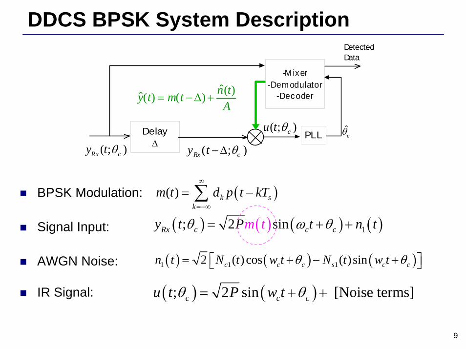
BPSK Modulation:
Signal Input:
AWGN Noise:
IR Signal:
DDCS BPSK System Description
( ) ( ) ( ) ( )1; 2 sinRx c c cy ntt mP t tθ ω θ= + +
( ) ( ) ( )1 1 12 ( ) cos ( )sinc c c s c cn t N t w t N t w tθ θ= + − +⎡ ⎤⎣ ⎦
( )( ) k sk
m t d p t kT∞
=−∞
= −∑
( ) ( ); 2 sin [Noise terms]c c cu t P w tθ θ= + +
10
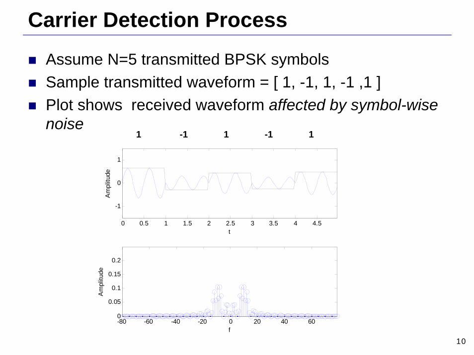
Carrier Detection Process
Assume N=5 transmitted BPSK symbolsSample transmitted waveform = [ 1, -1, 1, -1 ,1 ] Plot shows received waveform affected by symbol-wise noise
0 0.5 1 1.5 2 2.5 3 3.5 4 4.5
-1
0
1
t
Am
plitu
de
-80 -60 -40 -20 0 20 40 600
0.05
0.1
0.15
0.2
f
Am
plitu
de
1 -1 1 -1 1
11
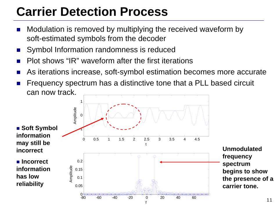
Carrier Detection ProcessModulation is removed by multiplying the received waveform by soft-estimated symbols from the decoderSymbol Information randomness is reducedPlot shows “IR” waveform after the first iterationsAs iterations increase, soft-symbol estimation becomes more accurateFrequency spectrum has a distinctive tone that a PLL based circuit can now track.
0 0.5 1 1.5 2 2.5 3 3.5 4 4.5
-1
0
1
t
Am
plitu
de
-80 -60 -40 -20 0 20 40 600
0.05
0.1
0.15
0.2
f
Am
plitu
de
Soft Symbol informationmay still beincorrect
Incorrect information has lowreliability
Unmodulatedfrequency spectrum begins to show the presence of a carrier tone.
12
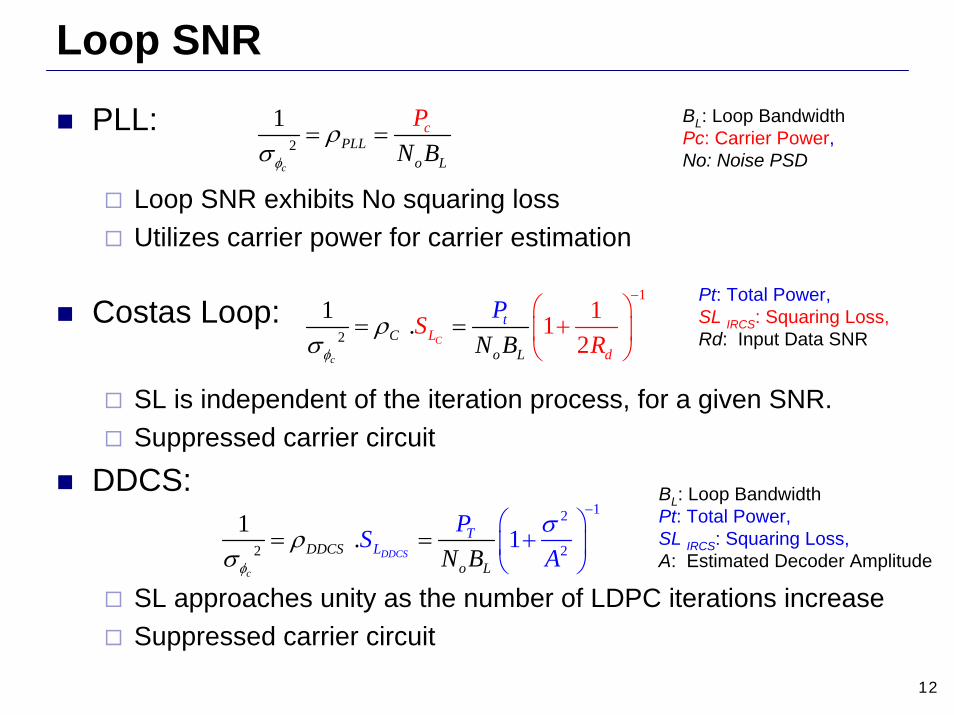
PLL:
Loop SNR exhibits No squaring lossUtilizes carrier power for carrier estimation
Costas Loop:
SL is independent of the iteration process, for a given SNR.Suppressed carrier circuit
DDCS:
SL approaches unity as the number of LDPC iterations increaseSuppressed carrier circuit
Loop SNR
2
1
c
PLLo L
cPN Bφ
ρσ
= =
2
111
2. 1
c
CCo
LdL
t
NS
BP
Rφ
ρσ
−⎛ ⎞+⎜= ⎟
⎝ ⎠=
2
12
211 .c
DDCSDDCS Lo L
TPAN B
Sφ
ρ σσ
−⎛ ⎞+⎜ ⎟
⎝ ⎠= =
BL: Loop BandwidthPt: Total Power,SL IRCS: Squaring Loss,A: Estimated Decoder Amplitude
BL: Loop BandwidthPc: Carrier Power,No: Noise PSD
Pt: Total Power,SL IRCS: Squaring Loss,Rd: Input Data SNR
13
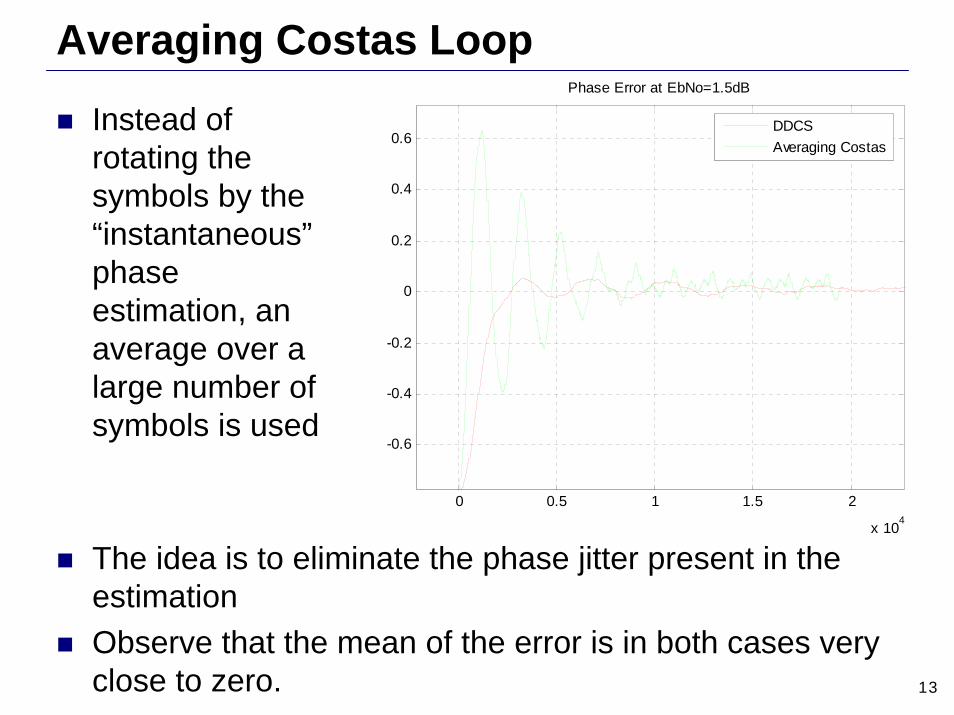
Averaging Costas Loop
The idea is to eliminate the phase jitter present in the estimationObserve that the mean of the error is in both cases very close to zero.
0 0.5 1 1.5 2
x 104
-0.6
-0.4
-0.2
0
0.2
0.4
0.6
Phase Error at EbNo=1.5dB
DDCSAveraging Costas
Instead of rotating the symbols by the “instantaneous”phase estimation, an average over a large number of symbols is used
14
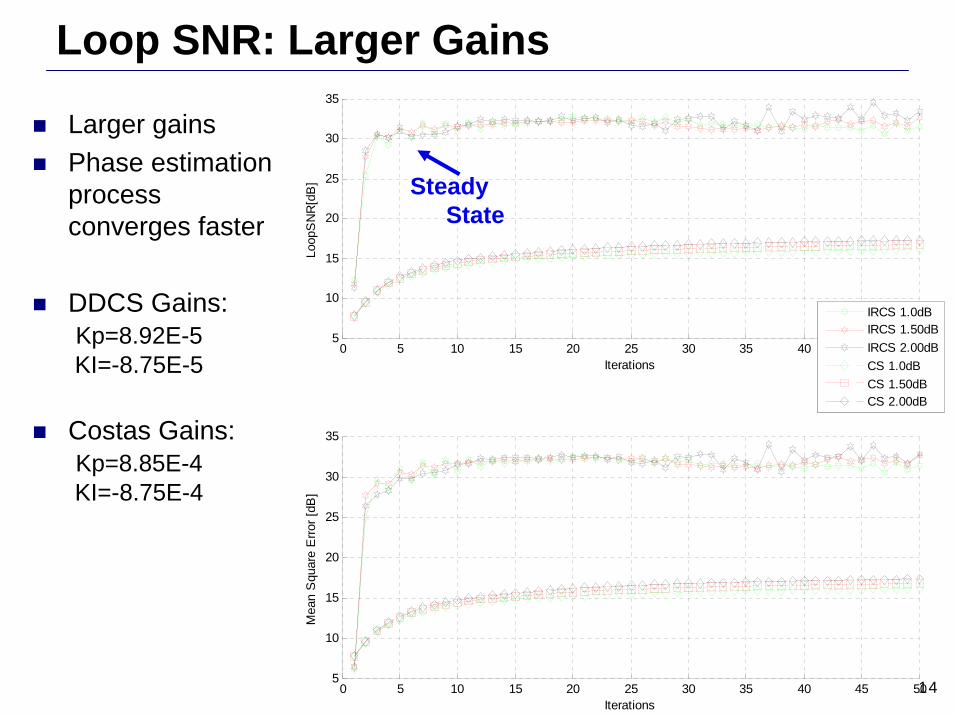
Loop SNR: Larger Gains
Larger gainsPhase estimation process converges faster
DDCS Gains:Kp=8.92E-5KI=-8.75E-5
Costas Gains:Kp=8.85E-4KI=-8.75E-4
0 5 10 15 20 25 30 35 40 45 505
10
15
20
25
30
35
Loop
SN
R[d
B]
Iterations
0 5 10 15 20 25 30 35 40 45 505
10
15
20
25
30
35
Mea
n S
quar
e E
rror [
dB]
Iterations
IRCS 1.0dBIRCS 1.50dBIRCS 2.00dBCS 1.0dBCS 1.50dBCS 2.00dB
SteadyState
15
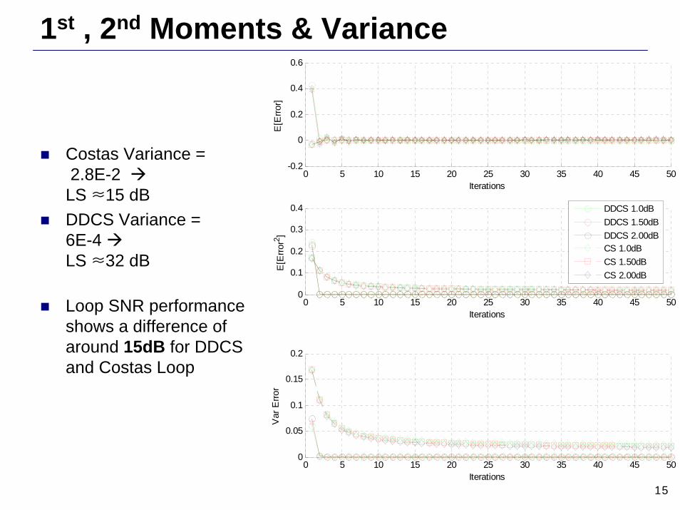
1st , 2nd Moments & Variance
Costas Variance =2.8E-2 LS ≈15 dBDDCS Variance = 6E-4 LS ≈32 dB
Loop SNR performance shows a difference of around 15dB for DDCS and Costas Loop
0 5 10 15 20 25 30 35 40 45 50-0.2
0
0.2
0.4
0.6
E[E
rror]
Iterations
0 5 10 15 20 25 30 35 40 45 500
0.1
0.2
0.3
0.4
E[E
rror2 ]
Iterations
DDCS 1.0dBDDCS 1.50dBDDCS 2.00dBCS 1.0dBCS 1.50dBCS 2.00dB
0 5 10 15 20 25 30 35 40 45 500
0.05
0.1
0.15
0.2
Var
Erro
r
Iterations
16
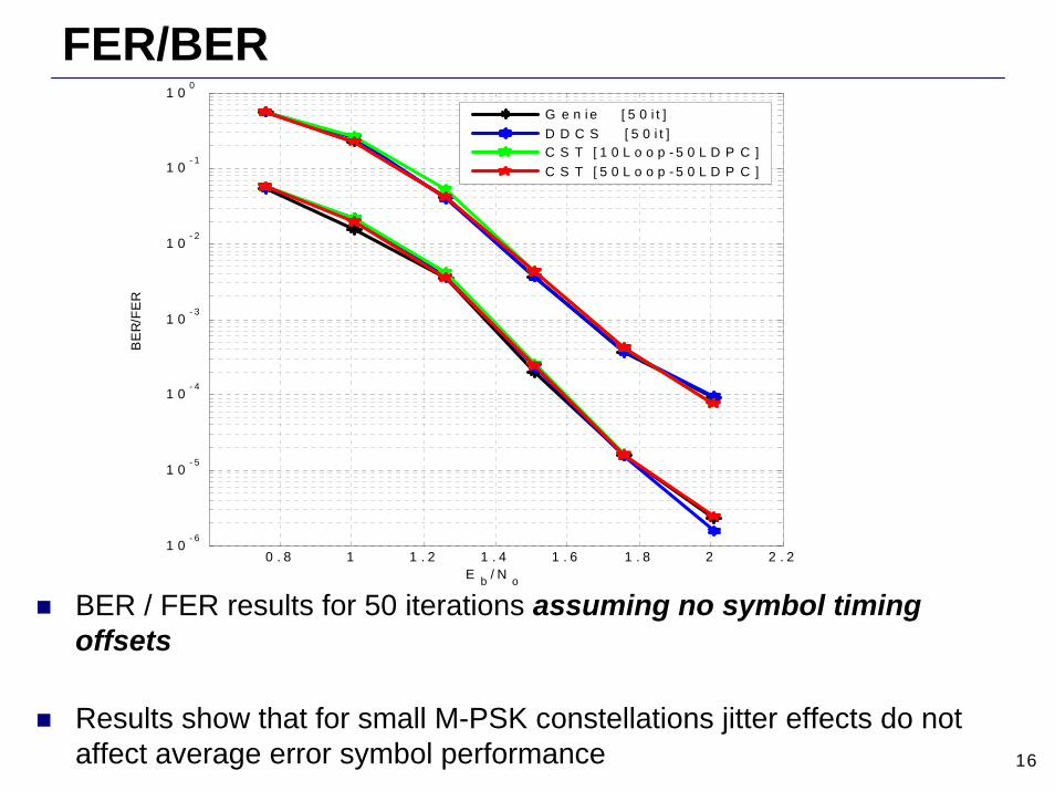
FER/BER
0 . 8 1 1 . 2 1 . 4 1 . 6 1 . 8 2 2 . 21 0
- 6
1 0- 5
1 0- 4
1 0- 3
1 0- 2
1 0- 1
1 00
E b / N o
BE
R/F
ER
G e n i e [ 5 0 i t ]D D C S [ 5 0 i t ]C S T [ 1 0 L o o p - 5 0 L D P C ]C S T [ 5 0 L o o p - 5 0 L D P C ]
BER / FER results for 50 iterations assuming no symbol timing offsets
Results show that for small M-PSK constellations jitter effects do not affect average error symbol performance
17
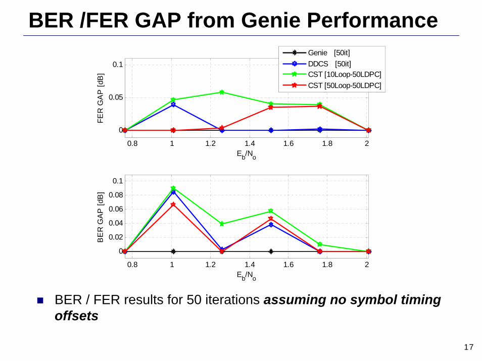
BER /FER GAP from Genie Performance
0.8 1 1.2 1.4 1.6 1.8 2
0
0.05
0.1
FER
GA
P [d
B]
Eb/No
Genie [50it]DDCS [50it]CST [10Loop-50LDPC]CST [50Loop-50LDPC]
0.8 1 1.2 1.4 1.6 1.8 2
0
0.02
0.04
0.06
0.08
0.1
BE
R G
AP
[dB
]
Eb/No
BER / FER results for 50 iterations assuming no symbol timing offsets
18
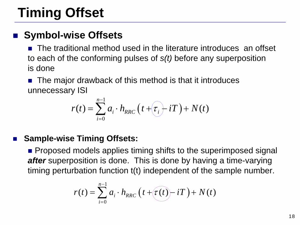
Symbol-wise OffsetsThe traditional method used in the literature introduces an offset
to each of the conforming pulses of s(t) before any superposition is done
The major drawback of this method is that it introduces unnecessary ISI
Sample-wise Timing Offsets:Proposed models applies timing shifts to the superimposed signal
after superposition is done. This is done by having a time-varying timing perturbation function t(t) independent of the sample number.
( )1
0
( ) ( ) ( )n
i RRCi
r t a h t t iT N tτ−
=
= ⋅ + − +∑
( )1
0( ) ( )
n
i RRC ii
r t a h t iT N tτ−
=
= ⋅ + − +∑
Timing Offset
19
Timing Offset
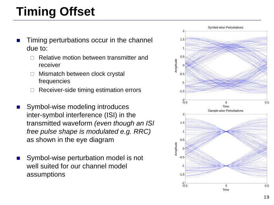
Timing perturbations occur in the channel due to:
Relative motion between transmitter and receiverMismatch between clock crystal frequenciesReceiver-side timing estimation errors
Symbol-wise modeling introduces inter-symbol interference (ISI) in the transmitted waveform (even though an ISI free pulse shape is modulated e.g. RRC)as shown in the eye diagram
Symbol-wise perturbation model is not well suited for our channel model assumptions
-0.5 0 0.5-2
-1.5
-1
-0.5
0
0.5
1
1.5
2
Time
Am
plitu
de
Symbol-wise Perturbations
-0.5 0 0.5-2
-1.5
-1
-0.5
0
0.5
1
1.5
2
Time
Am
plitu
de
Sample-wise Perturbations
20
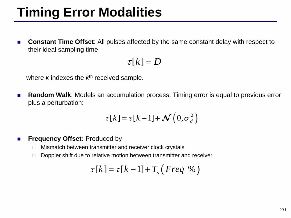
Timing Error Modalities
Constant Time Offset: All pulses affected by the same constant delay with respect totheir ideal sampling time
where k indexes the kth received sample.
Random Walk: Models an accumulation process. Timing error is equal to previous error plus a perturbation:
Frequency Offset: Produced by Mismatch between transmitter and receiver clock crystalsDoppler shift due to relative motion between transmitter and receiver
( )2[ ] [ 1] 0, dk kτ τ σ= − +N
[ ]k Dτ =
( )[ ] [ 1] %sk k T Freqτ τ= − +
21
-2 -1 0 1 2 3 4 5 6 7 8-2
0
2(b) Transmitted Waveform
Am
plitu
de
Time
-2 -1 0 1 2 3 4 5 6 7 8-5
0
5(a) Perturbation Profile
Tim
ing
Offs
et
Time
-2 -1 0 1 2 3 4 5 6 7 8-2
0
2(c) Received W aveform
Am
plitu
de
Time
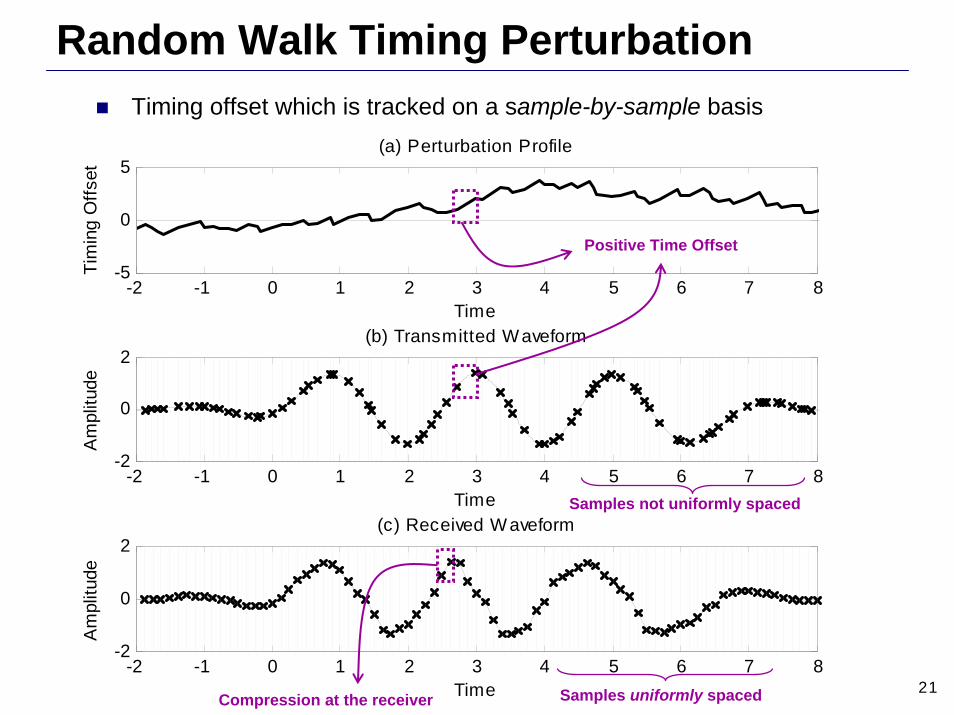
Random Walk Timing Perturbation
Samples not uniformly spaced
Samples uniformly spaced
Positive Time Offset
Compression at the receiver
Timing offset which is tracked on a sample-by-sample basis
22
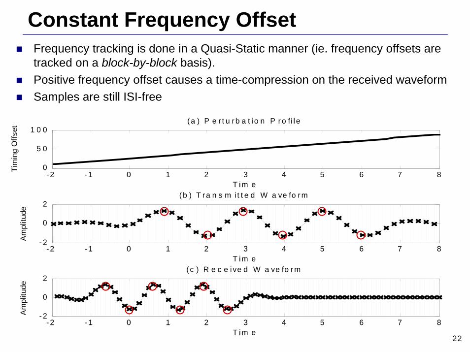
Constant Frequency Offset
- 2 -1 0 1 2 3 4 5 6 7 8-2
0
2(b ) T ra n s m i t t e d W a ve fo rm
Am
plitu
de
T im e
-2 -1 0 1 2 3 4 5 6 7 80
5 0
1 0 0(a ) P e r t u rb a t io n P ro fi l e
Tim
ing
Offs
et
T im e
-2 -1 0 1 2 3 4 5 6 7 8-2
0
2(c ) R e c e ive d W a ve fo rm
Am
plitu
de
T im e
Frequency tracking is done in a Quasi-Static manner (ie. frequency offsets are tracked on a block-by-block basis). Positive frequency offset causes a time-compression on the received waveformSamples are still ISI-free
23
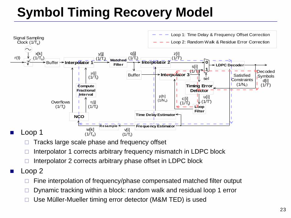
Symbol Timing Recovery Model
Loop 1Tracks large scale phase and frequency offsetInterpolator 1 corrects arbitrary frequency mismatch in LDPC blockInterpolator 2 corrects arbitrary phase offset in LDPC block
Loop 2Fine interpolation of frequency/phase compensated matched filter outputDynamic tracking within a block: random walk and residual loop 1 errorUse Müller-Mueller timing error detector (M&M TED) is used
r(t)Interpolator 1
Signal SamplingClock (1/Ts)
x[k](1/Ts) Matched
Filter
y[j](1/Ti)
z[i](1/T')
LDPC Decoder
ComputeFractional
Interval
μ[j](1/Ti)
η [j](1/Ti)
NCO
R esample
Overflows(1/Ti)
w[k](1/Ts)
v[i](1/Ti)
q[j](1/Ti)
01
Buffer
Loop 1: Time Delay & Frequency Offset Correction
Frequency Estimator
Time Delay Estimator
Interpolator 2
SatisfiedConstraints
(1/Nc)
p[h](1/Nv)
Timing ErrorDetector
DecodedSymbols
d[i](1/T')
Buffer
u[i](1/T')
LoopFilter
sel
s[i](1/Ti)
c[i](1/Ti)
Interpolator 3
Loop 2: Random Walk & Residue Error Correction
24
-1200 -800 -400 0 400 800 1200
Estimate [ppm]
Satis
fied
Con
stra
ints
-1600 1600
BestEstim ate800ppm
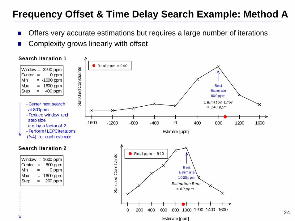
Window = 3200 ppmCenter = 0 ppmMin = -1600 ppmMax = 1600 ppmStep = 400 ppm
Search Ite ration 1
- Center next search at 800ppm- Reduce window and step size e.g. by a factor of 2- Perform l LDPC iterations (l<4) for each estimate
600 800
Estimate [ppm]
Satis
fied
Con
stra
ints
Search Ite ration 2
200 4000 16001200 14001000
BestEstim ate1000ppm
Real ppm = 940
Window = 1600 ppmCenter = 800 ppmMin = 0 ppmMax = 1600 ppmStep = 200 ppm
Estimation Error= 140 ppm
Estimation Error= 60 ppm
Real ppm = 940
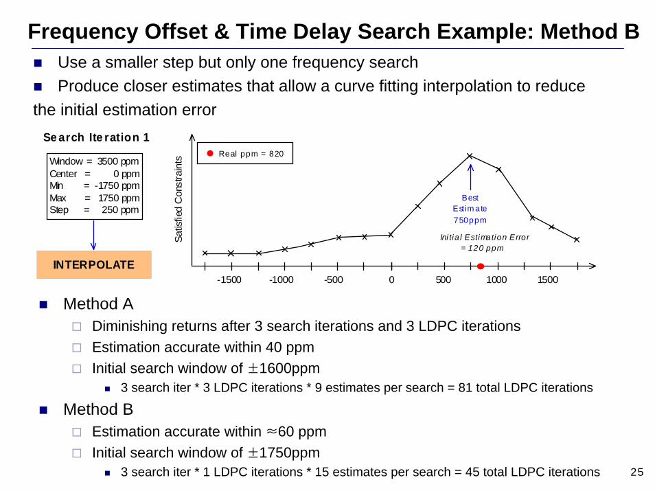
Frequency Offset & Time Delay Search Example: Method A
Offers very accurate estimations but requires a large number of iterationsComplexity grows linearly with offset
25
-1000 -500 0 1000
Satis
fied
Con
stra
ints
1500
BestEstim ate750ppm
Window = 3500 ppmCenter = 0 ppmMin = -1750 ppmMax = 1750 ppmStep = 250 ppm
Se arch Ite ration 1
INTERPOLATE
Real ppm = 820
Ini tia l Estimation Error= 120 ppm×
-1500 500
Frequency Offset & Time Delay Search Example: Method BUse a smaller step but only one frequency searchProduce closer estimates that allow a curve fitting interpolation to reduce
the initial estimation error
Method ADiminishing returns after 3 search iterations and 3 LDPC iterationsEstimation accurate within 40 ppmInitial search window of ±1600ppm
3 search iter * 3 LDPC iterations * 9 estimates per search = 81 total LDPC iterations
Method BEstimation accurate within ≈60 ppmInitial search window of ±1750ppm
3 search iter * 1 LDPC iterations * 15 estimates per search = 45 total LDPC iterations
26
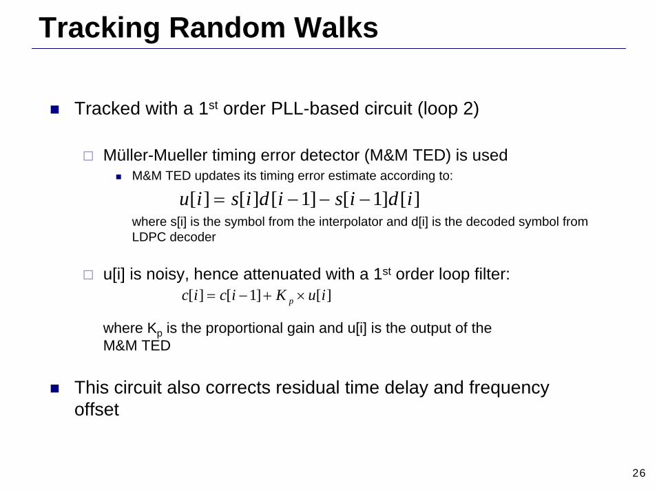
Tracking Random Walks
Tracked with a 1st order PLL-based circuit (loop 2)
Müller-Mueller timing error detector (M&M TED) is usedM&M TED updates its timing error estimate according to:
where s[i] is the symbol from the interpolator and d[i] is the decoded symbol from LDPC decoder
u[i] is noisy, hence attenuated with a 1st order loop filter:
where Kp is the proportional gain and u[i] is the output of the M&M TED
This circuit also corrects residual time delay and frequency offset
][]1[]1[][][ idisidisiu −−−=
][]1[][ iuKicic p ×+−=
27
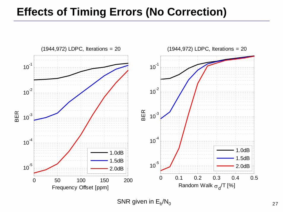
Effects of Timing Errors (No Correction)
0 50 100 150 200
10-5
10-4
10-3
10-2
10-1
(1944,972) LDPC, Iterations = 20
Frequency Offset [ppm]
BE
R
1.0dB1.5dB2.0dB
0 0.1 0.2 0.3 0.4 0.5
10-5
10-4
10-3
10-2
10-1
(1944,972) LDPC, Iterations = 20
Random Walk σd/T [%]
BE
R1.0dB1.5dB2.0dB
SNR given in Eb/N0
28
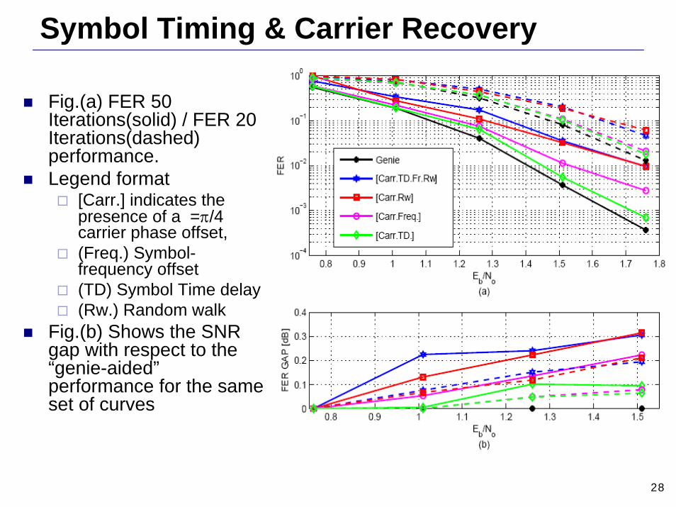
Symbol Timing & Carrier Recovery
Fig.(a) FER 50 Iterations(solid) / FER 20 Iterations(dashed) performance.Legend format
[Carr.] indicates the presence of a =π/4 carrier phase offset,(Freq.) Symbol-frequency offset(TD) Symbol Time delay(Rw.) Random walk
Fig.(b) Shows the SNR gap with respect to the “genie-aided”performance for the same set of curves
29
SummaryCarrier synchronization circuit overcomes the performance loss due to a noisy signal reference at low SNRs, characteristic of suppressed carrier loops such as the Costas loop.Steady state operation is reached after around 15 joint DDCS/LDPC iterations.Two-stage pilotless symbol timing recovery model for tracking time delay, frequency offsets and random walks1st stage: LDPC constraint feedback to track large-scale time delays and symbol frequency offsets Windowed search method
Complexity grows linearly with offsetCan track any time delay frequency offset as long as it is within the initial search window
2nd stage: decoded LDPC symbols to track random walks and residual errors from the 1st stageSimulations results show within 0.4 dB of the ideal code performance for time delays and frequency offsets
Recommended