Beam-Forming and Power Control in
Flexible Spectrum Usage for LTE
Advanced System
Aalborg University
Institute of Electronic Systems
Department of Communication Technology
Project Group 1124, 2008
2
Aalborg University
Institute of Electronic Systems
Department of Communication Technology
Fredrik Bajers VEJ 7, DK-9220 Aalborg Øst. Phone: +45 96358700
TITLE: Beam-Forming and Power Control in Flexible
Spectrum Usage for LTE Advance System
PROJECT PERIOD: October 2007 to May 2008
PROJECT GROUP: MOBCOM - 1124
AUTHOR: Massimiliano Ricci
SUPERVISORS: Nicola Marchetti
Shashi Kant
NUMBER OF PAGES: 98
This report must not be published or reproduced without permission from the author
Copyright © 2008, Aalborg University

3
4
Abstract
Beamforming and power control algorithms are investigated in intra-system spectrum sharing for
LTE Advanced system (named as Flexible Spectrum Usage, FSU) context.
FSU is considered to occupy scarce spectral resources opportunistically in order to increase the
average spectral efficiency of the system and to provide less interference to the other system. So, to
avoid interference to other systems, beamforming and power control algorithms are investigated
and implemented in MATLAB. As a starting point, assuming perfect channel state information at the
transmitter, single-user (SU) multiple input multiple output (MIMO) downlink beamforming is
implemented to evaluate the link performance of the system. As a case study, a link-level simulator
complying UTRAN Long Term Evolution (LTE) standard is considered. Moreover, two multi-user
(MU) MIMO downlink with OFDM/SDMA access scheme, beamforming algorithms zero-forcing
(ZF) and successive minimum mean square error (SMMSE) are investigated to evaluate
performance of the system at link-level by averaging the bit error rates (BERs) and throughputs
(THs) of all the candidate users. Dominant eigen transmission (DET) power algorithm is to applied
to both to maximize the SNR at the receiver and to minimize the BER. Numerical simulation results
show significant gains by 3dB to 5 dB, depending of the modulation using, and 3dB about, for the
low SNR, for the considered 22× system in terms of BER and TH, respectively, compared to the
same considered system without beamforming. Other results show significant gains by 3 dB and 3
dB, in terms of BER and TH, respectively, comparing SMMSE to ZF beamforming algorithm.

5
Dedication
To my parents

6
Abbreviations
3GPP Third Generation Partnership Project
ADC Analog-to-Digital Converter
BER Bit Error Rate
BF Beam-Forming
CCI Co-Channel Interference
CDMA Code-Division Multiplexing Access
CP Cyclic Prefix
CR Cognitive Radio
CSI Channel State Information
CSIT Channel State Information at the Transmitter
DAC Digital-to-Analog Converter
DET Dominant Eigenmode Transmission
DFT Discrete Fourier Transform
DOA Direction Of Arrival
ECR Effective Coding Rate
FDD Frequency-Division Duplexed
FDM Frequency-Division Multiplexing
FDMA Frequency-Division Multiplexing Access
FFT Fast Fourier Transform
FSU Flexible Spectrum Use
HNB Home Node B
HT Hilly Terrain
ICI Inter-Carrier Interference
IDFT Inverse Discrete Fourier Transform
IFFT Inverse Fast Fourier Transform
IMT-A International Mobile Telecommunications-Advanced
ISI Inter-Symbol Interference
ITU International Telecommunications Union
LA Local Area
LOS Line of Sight
LTE Long Term Evolution

7
MA Metropolitan Area
MIMO Multiple-Input Multiple-Output
MISO Multiple-Input Single-Output
MMSE Minimum Mean Square Error
MU Multi User
MUI Multi User Interference
OFDM Orthogonal Frequency-Division Multiplexing
OFDMA Orthogonal Frequency-Division Multiplexing Access
PC Power Control
PRB Physical Resource Block
PtoS Parallel to Serial
QoS Quality of Service
RA Rural Area
SDMA Space-Division Multiplexing Access
SEL Spectral Efficiency Loss
SISO Single-Input Single-Output
SM Spatial Multiplexing
SMMSE Successive Minimum Mean Square Error
SNR Signal-to-Noise Ratio
SS Spectrum Sharing
StoP Serial to Parallel
SU Single User
SVD Singular Value Decomposition
TC Turbo Coding
TDD Time-Division Duplexing
TDMA Time-Division Multiplexing Access
TTI Transmission Time Interval
TU Typical Urban
UE User Equipment
WA Wide Area
WF Water Filling
ZF Zero Forcing
8
List of Figures
Figure 1. Simplified Cognitive Cycle [1].......................................................................................... 19
Figure 2. Classification of SS............................................................................................................ 21
Figure 3. Inter-Network SS and Intra-Network SS........................................................................... 22
Figure 4. Frequency-Time representation of an OFDM signal......................................................... 24
Figure 5. Modulation of each sub-carrier.......................................................................................... 24
Figure 6. Conceptual OFDM transmitter .......................................................................................... 25
Figura 7. OFDM transmitter with IFFT........................................................................................... 26
Figure 8. Cyclic Prefix avoiding ISI ................................................................................................. 27
Figure 9. Cyclic prefix as a copy of the last part of an OFDM symbol ............................................ 27
Figure 10. OFDM block diagram...................................................................................................... 29
Figure 11. OFDMA downlink block diagram................................................................................... 30
Figure 12. Example of OFDM with multiple access......................................................................... 31
Figure 13. MU-OFDM with FDMA ................................................................................................. 32
Figure 14. OFDM/FDMA variations ................................................................................................ 32
Figure 15. MU-OFDM with TDMA................................................................................................. 33
Figure 16. System model in OFDM/SDMA ..................................................................................... 34
Figure 17. MU-OFDM with SDMA ................................................................................................. 35
Figure 18. Polar diagram of a typical antenna beampattern.............................................................. 36
Figure 19. A generic BF antenna system ......................................................................................... 37
Figure 20. Signal output array [13] ................................................................................................... 37
Figure 21. Introduction of the weight to calculate the just direction of the signal [13].................... 38
Figure 22. Beamforming for processing narrowband signals. .......................................................... 39
Figure 23. Beamforming for processing broadband signals. ............................................................ 40

9
Figure 24. Beamforming performed in the frequency domain for the broadband signals................ 40
Figure 25. Adaptive beamforming for SDMA.................................................................................. 42
Figure 26. MIMO configuration ....................................................................................................... 45
Figure 27. Scenario representation.................................................................................................... 48
Figure 28. Conceptual diagram of downlink system ........................................................................ 50
Figure 29. TDD frame structure in LTE for OFDM with 1o ms radio frame duration .................... 51
Figure 30. Block diagram of MU case for DL transmission............................................................. 53
Figure 31. Block diagram for linear transmission model for multi-user MIMO beamforming........ 55
Figure 32. UncodedBER Beamforming vs. no Beamforming with QPSK modulation.................... 70
Figure 33. CodedBER Beamforming vs. no Beamforming with QPSK modulation........................ 70
Figure 34. Throughput Beamforming vs. no Beamforming with QPSK modulation....................... 71
Figure 35. UncodedBER Beamforming vs. no Beamforming with 16-QAM modulation ............... 71
Figure 36. CodedBER Beamforming vs. no Beamforming with 16-QAM modulation ................... 72
Figura 37.Throughput Beamforming vs. no Beamforming with 16-QAM modulation ................... 72
Figure 38. UncodedBER ZF vs SMMSE......................................................................................... 74
Figure 39. CodedBER ZF vs SMMSE.............................................................................................. 74
Figure 40. Throughput ZF vs SMMSE ............................................................................................. 75
Figure 41. CodedBER SMMMSE+PC vs. SMMSE.........................................................................76
Figure 42. Throughput SMMSE+PC vs. SMMSE............................................................................ 77
Figure 43. Duplexing in CSI ............................................................................................................. 93
10
List of Tables
Table 1. Parameters for downlink transmission scheme ................................................................... 52
Table 2. Typical Urban relative delays and powers........................................................................... 89
Table 3. UL and DL data rates in LTE.............................................................................................. 90

11
12
Table of Content
Chapter 1
1. Introduction 14
1.1. Organization of this Thesis 16
Chapter 2
2. Background 18
2.1 Cognitive Radio 19
2.1.1 Spectrum Sharing 21
2.2 OFDM 24
2.3 Multi Access with OFDM 30
2.3.1 OFDM/FDMA (OFDMA) 31
2.3.2 OFDM/TDMA 33
2.3.3 OFDM/SDMA 34
2.4 Beamforming 36
2.4.1 Beamforming-Based SDMA 42
2.5 MIMO System 44
Chapter 3
3. Project description 48
3.1 Scenario 49
3.2 System Architecture for LTE 51
3.2.1 Transmitter architecture 52
3.2.2 Channel model 54
3.2.3 Receive architecture 55
Chapter 4
4. Beamforming methods 58
4.1 Zero-Forcing (ZF) 60
4.2 Successive Minimum Mean Square Error (SMMSE) 62
4.3 Dominant Eigenmode Transmission (DET) Power Control 65
13
Chapter 5
5. Simulation Results 67
5.1 Parameters of the Simulation 68
5.2 Beamforming for Single User 69
5.3 Beamforming for Multi-User 73
5.4 Beamforming for Multi-User with Power Control 76
Chapter 6
6. Conclusion and Future work 79
6.1 Conclusion 80
Bibliography 83
Appendix A 88
Channel Profiles 88
Appendix B 90
LTE context 90
Appendix C 92
TDD System 92
Acknowledgement 94
14
Chapter 1
1. Introduction
In the recent years, the International Telecommunications Union (ITU) is working on specifying the
system requirements towards next generation mobile communication systems, called International
Mobile Telecommunications-Advanced (IMT-A), [27]. The deployment of IMT-A systems is
believed to take place at mass market level around year 2015 and will realize what has been a
buzzword for almost a decade, namely “4G”. The 4G radio network concept (Cognitive Radio, CR
[1], [2]) covers the full range of operability scenario from Wide Area (WA) over Metropolitan Area
(MA) to Local Area (LA). IMT-A systems are expected to provide peak data-rates in the order of
Gpbs1 in LA. Such data-rates require usage of Multiple-Input Multiple-Output (MIMO)
technology [15], [16], to achieve high spectral efficiency and a very wide spectrum allocation in the
range of MHz100 . In MIMO communications systems, multiple antenna are used at both sides of
the link.
An important research topic is the study of Multi-User (MU) MIMO systems [17]. With a high
number of users it will become even more difficult to identify exclusive spectrum for all user. To
solve this problem, together with the MIMO technology, users are needed also to coexist in the
same spectrum in an efficient way. This is possible considering a Flexible Spectrum Use (FSU)
[28], [29]. The major advantage of FSU is a better spectral scalability of the system compared to
classic spectrum management techniques. In this way, in a LA scenario with one cell and one Home
Node B (HNB), different users can coexist on the on the same frequency-time domain. This is
possible considering as multiple access scheme the Orthogonal Frequency Division Multiplexing
(OFDM) with Space Division Multiple Access (SDMA) [6] - [11]. It has been chosen as multiple
access for downlink in Long Term Evolution (LTE). Such systems have the potential to combine the
high capacity achievable with MIMO processing with the benefits of SDMA. SDMA is an advanced
transmission technique, where MU are signalled on the same time and same frequency resource; it is
15
used to enhance the spectral efficiency. So, a large number of User Equipments (UEs) share the
whole spectrum. In this scheme HNB prepares a number of directional beams to cover the UEs area.
Beamforming (BF) [12], [13] concentrates transmit power to a desired direction and reduces power
emissions to undesired directions; this way BF eliminate Multi-User Interference (MUI) caused by
all others UEs.
BF and power control (PC) algorithms for MIMO-OFDM/SDMA LTE advanced systems in the
FSU context are investigated and implemented in MATLAB. To implement downlink BF algorithm,
HNB need the knowledge of the Channel State Information (CSI). CSI are obtained by a Time-
Division Duplexing (TDD) systems.
In TDD system, uplink and downlink transmission are time duplexed over the same frequency
bandwidth. Using the reciprocity principle it is possible to use the estimated uplink channel for
downlink transmission.
We consider two algorithms for downlink BF: Successive Minimum Mean Square Error
(SMMSE) [14], [20], [21] and Zero Forcing (ZF) [14], [19], [20]. SMMSE transmits beamforming
treats; each receive antenna separately, and it has the advantage that the total number of receiving
antennas at the users’ terminals may be greater than the number of antennas at the HNB. In ZF, the
signal of each user is pre-processed at the transmitter, using a modulation matrix that lies in the null
space of all other users’ channel matrices; so, the MUI in the system is forced to zero.
PC is also investigated, it’s considered a Dominant Eigenmode Transmission (DET) algorithm
which transmits just on the dominant eigenmode of each UE. It provides to maximize the Signal
Noise Ratio (SNR) at the receivers and to minimize the Bit Error Rate (BER).
As a starting point, assuming perfect channel state information at the transmitter, single-user (SU)
multiple input multiple output (MIMO) downlink beamforming is implemented to evaluate the link
performance of the system. As a case study, a link-level simulator complying UTRAN Long Term
Evolution (LTE) standard is considered. Moreover, two multi-user (MU) MIMO downlink with
OFDM/SDMA access scheme, beamforming algorithms zero-forcing (ZF) and successive minimum
mean square error (SMMSE) are investigated to evaluate performance of the system at link-level by
averaging the bit error rates (BERs) and throughputs (THs) of all the candidate users. Dominant
eigen transmission (DET) power algorithm is to applied to both to maximize the SNR at the receiver
and to minimize the BER.
BF and PC eliminate the MUI and minimize the total transmitted power and this is exactly the
problem that will be considered here, i.e. how to choose the transmit BF vectors so that the total
transmitted power is minimized while the system provides an acceptable Quality of Service (QoS)
to as many users as possible.
16
1.1. Organization of this Thesis
This report documents a master thesis in Telecommunication Engineering done in the Mobile
Communication Division, Department of Communication Technology, Institute of Electronic
System, Aalborg University (AAU), in Denmark; in collaboration with INFOCOM Department,
Facoltà di Ingegneria, La Sapienza University Rome, in Italy, which the author is member.
This thesis is organized as follows:
Chapter II gives the background theory about localization techniques and data fusion method. It
states the fundamentals of the Cognitive Radio, of the OFDM technology, including the signal
generation and reception; of the OFDM multi-user access. In addition, it introduces the BF concept
and the MIMO technology.
Chapter III presents the project description: scenario, problem definition, system architecture, scope
of the project and the necessary assumptions.
Chapter IV introduces the BF methods (SMMSE and ZF) utilized and the Power Control method
(DET).
Chapter V presents the parameter utilized in the simulations and the results obtained for a single-
user system and a multi-user system.
Chapter VI summarizes the achievements reached during this thesis. Future work will be also be
presented.

17
18
Chapter 2
2. Background
This chapter provides technical background that is essential to the thesis. First, it includes an
overview on the Cognitive Radio, in particular the function of the Spectrum Sharing, which
provides control and access techniques in order to guarantee a free interference communication
among several different terminals.
Second, it includes an overview on the OFDM and multi access with OFDM systems; the OFDM
symbol (information bits) that are transmitted on a set of orthogonal subcarriers. In particular, it
treats various multiple access for the OFDM system: OFDM/FDMA (OFDMA), OFDM/TDMA,
OFDM/SDMA.
Third, it includes an overview on the Beamforming, in particular the beamforming-based SDMA
that we’ll use to try eliminate the interferences.
19
2.1 Cognitive Radio
The term Cognitive Radio (CR) was coined by Joseph Mitola [1] :
“A Cognitive Radio is a radio frequency transmitter/receiver that is designed to intelligently detect
whether a particular segment of the radio spectrum is currently in use, and to jump into (and out of,
if necessary) the temporarily-unused spectrum very rapidly, without interfering with the
transmission of other authorized users.”
“A Cognitive Radio is self-aware, user-aware, RF-aware, and that incorporates elements of
language technology and machine vision.”
The concept of a radio capable of adapting to the environment and to adjust transmission parameters
according to internal and external events is very important in the wireless world.
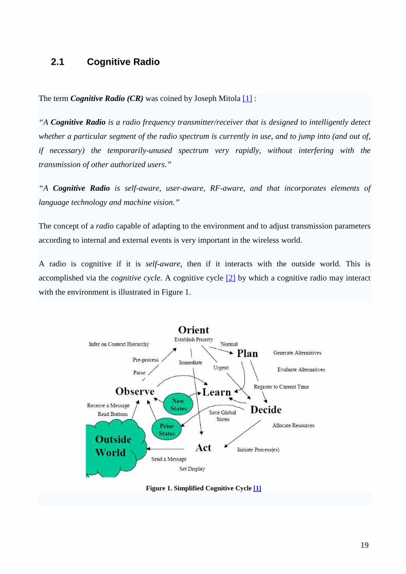
A radio is cognitive if it is self-aware, then if it interacts with the outside world. This is
accomplished via the cognitive cycle. A cognitive cycle [2] by which a cognitive radio may interact
with the environment is illustrated in Figure 1.
Figure 1. Simplified Cognitive Cycle [1]
20
A CR executes five main actions:
• Observe, cognitive radios are aware of their surrounding environment.
• Plan, cognitive radios evaluate among several strategies.
• Decide, cognitive radios are always capable to select one strategy of operation.
• Learn, cognitive radios can enrich experience by forming new strategies.
• Act, cognitive radios perform communication according to the selected strategy.
CR technology is expected to improve spectrum access through:
• Spectrum Sensing: monitoring and detecting the spectrum holes to reuse them properly,
with two different techniques: transmitter detection (the CR terminal decides if the frequency
band is free or is not by its own, through two different methods: Matched Filter and Energy
detector); cooperative detection (the CR terminal gets sensing information from other users
and potentially can reach better results than transmitter detection alone).
• Spectrum Management: once the device has monitored the radio environment, according to
the results of the monitoring, according to the service requirements (QoS), the cognitive
radio terminal must find out the frequency hole which suits better every single particular
transmission.
• Spectrum Mobility: the transmission frequency can dynamically change if the user signal
transmission shows up suddenly.
• Spectrum Sharing: it provides control and access techniques in order to guarantee an
interference free communication among several different terminals.
So, a Cognitive Radio should be able to determine the spectral characteristics of the radio
environment it operates in, and, if necessary, to change some transmission parameters. In particular,
CR approach has the potential to alleviate the limitations in the frequency, spatial and temporal
domains and provide for real-time spectrum access negotiation and transactions, thus facilitating
dynamic spectrum sharing. The problem is that in a spectrum sharing environment, we have a co-
channel interference caused by sharing the same radio channel. Power control and array
beamforming are two well-known approaches that control co-channel interference and thus improve
the system capacity.
21
2.1.1 Spectrum Sharing
Spectrum Sharing (SS) [22] is verified when independent radio system (like military radars,
cellular,…) or independent users use the same spectrum in co-operation (time, place, code and/or
event,…). The SS process consists of five major step:
• Spectrum sensing, an user can just allocate a portion of the spectrum if that portion
doesn’t used by an unlicensed user.
• Spectrum allocation, based on the spectrum availability, the node can then allocate a
channel.
• Spectrum access, it is possible that more nodes would access to the spectrum, this access
must be coordinate.
• Transmitter-receiver handshake, once a portion of the spectrum is determined for
communication the receiver of this communication should also be indicated about the
selected spectrum. So, a transmitter-receiver handshake protocol is needed.
• Spectrum mobility, nodes are considered as visitors to the spectrum they allocate.
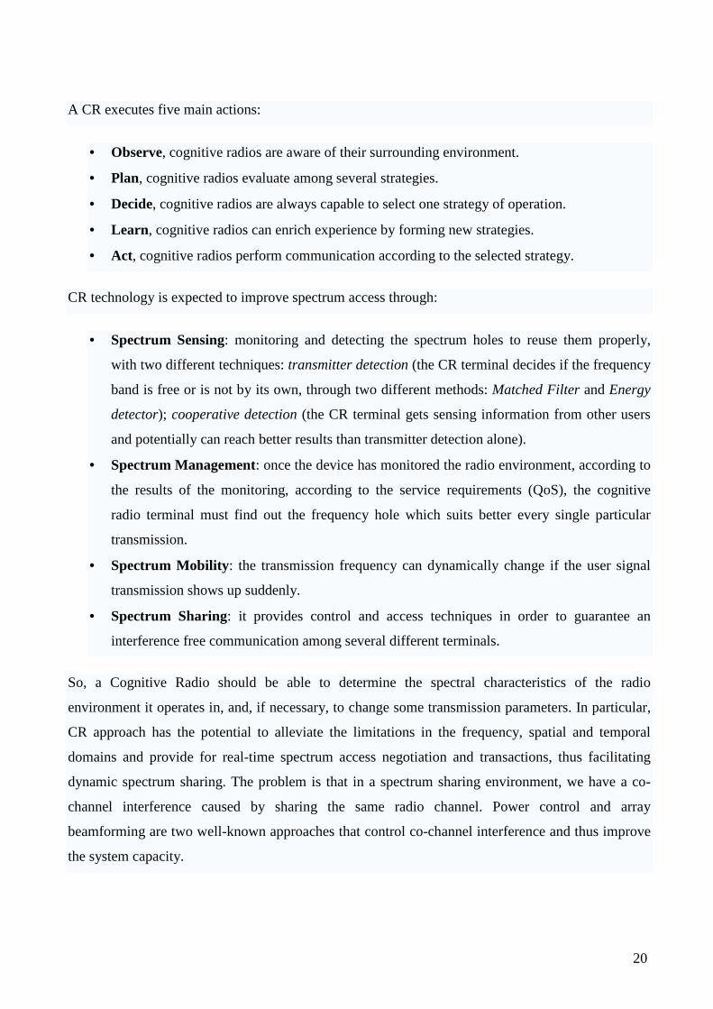
The classification of the SS is based on architecture, spectrum allocation behavior and spectrum
access technique as shown in Figure 2.
Figure 2. Classification of SS The first classification for SS technique is based on the architecture:
• Centralized spectrum sharing, a centralized entity controls the spectrum allocation and
access procedures.
• Distributed spectrum sharing, each node is responsible for the spectrum allocation and
access is based on local policies.
The second classification for SS techniques is based on the access behaviour:
22
• Cooperative spectrum sharing, it considers the effect of the node’s communication on the
other nodes, so the interference measurements of each node are shared among other modes.
• Non-cooperative spectrum sharing, it considers just the node at hand.
The third classification for SS technique is based on the access technology:
• Overlay spectrum sharing, a node accesses the network using a portion of the spectrum that
has not been used by licensed users.
• Underlay spectrum sharing, a node begins the transmission such that its transmit power at a
certain portion of the spectrum is considered as noise by the licensed users.
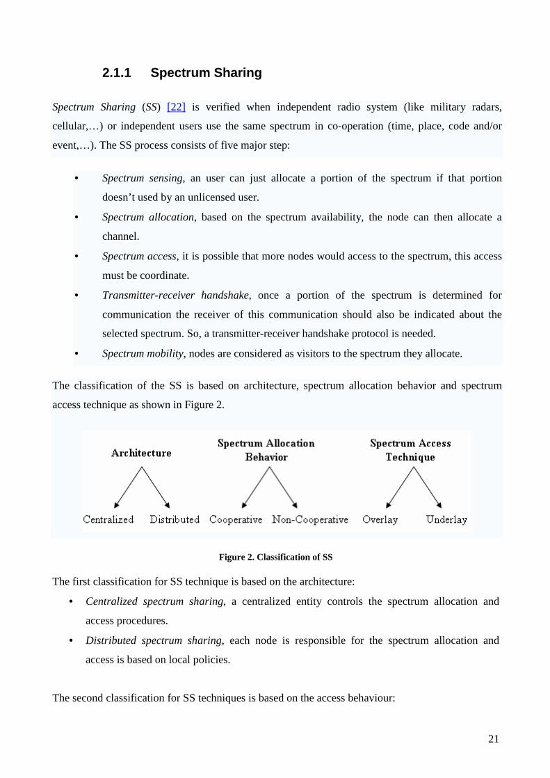
The networks analyzed to provide opportunistic access to the licensed spectrum using unlicensed
users. This causes SS among systems and we can have Inter-Network Spectrum Sharing and Intra-
Network Spectrum Sharing as shows in figure 8.
Figure 3. Inter-Network SS and Intra-Network SS
We treat just the Intra-Network SS, where the users try to access the available spectrum without
causing interference to others users. In particular, we are in the Flexible Spectrum Usage (FSU)
[28], [29], where the users are able to use spectrum in a flexible way by adapting their operation to

23
the current situation. The major advantage of FSU is a better spectral scalability of the system
compared to classic spectrum management techniques.
To facilitate FSU, the system shall dynamically be able to adapt frequency, time and space resource
over time in order to maximize the spectral efficiency with the constraint the Quality of Service
(QoS) requirements are met.
A multi access with OFDM is suitable candidate for FSU because if its flexible nature to support
spectrum sharing.
In this way, a MUI (Multi-User Interference) is generated by the presence of several users sharing a
some resource. To reduce the presence of MUI, we can use an orthogonal multiple access scheme,
that then implementing with the Power control and Beamforming technique can eliminate almost
totally the MUI.
24
2.2 OFDM
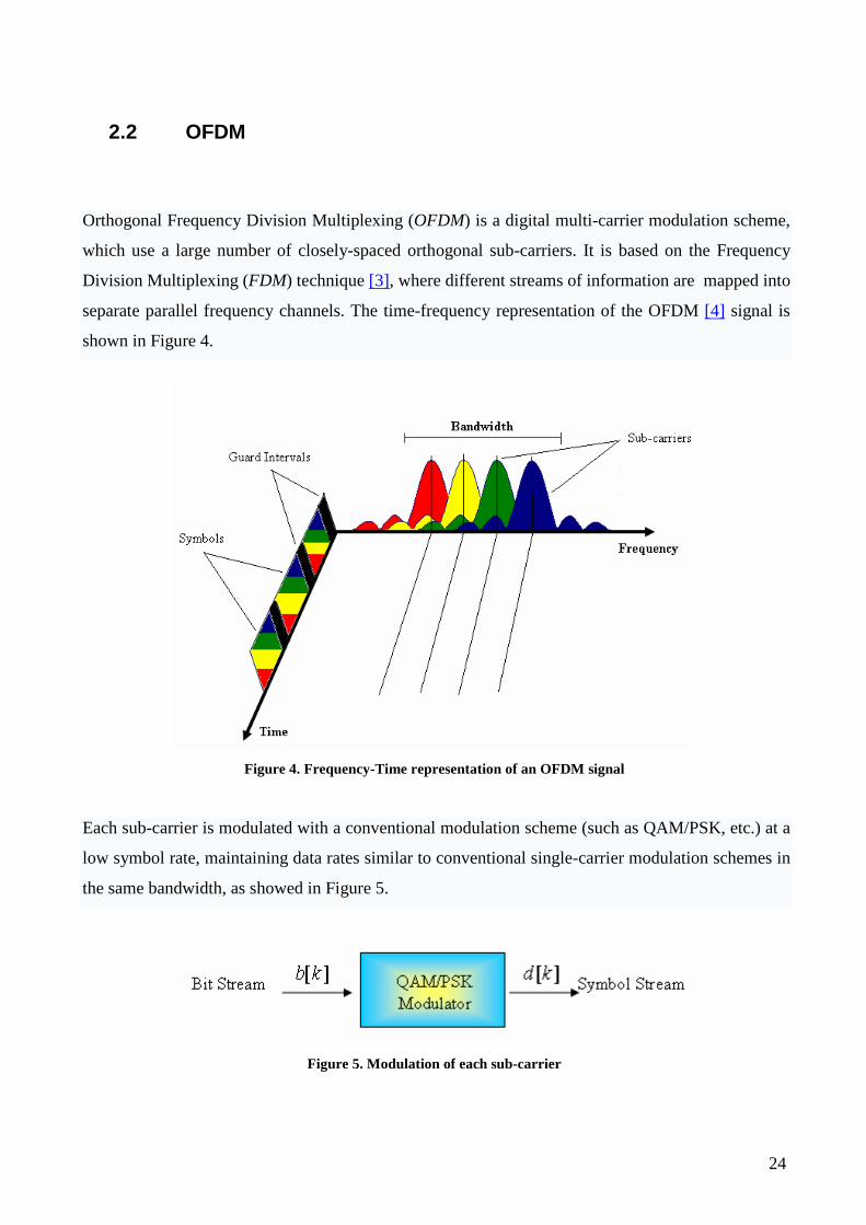
Orthogonal Frequency Division Multiplexing (OFDM) is a digital multi-carrier modulation scheme,
which use a large number of closely-spaced orthogonal sub-carriers. It is based on the Frequency
Division Multiplexing (FDM) technique [3], where different streams of information are mapped into
separate parallel frequency channels. The time-frequency representation of the OFDM [4] signal is
shown in Figure 4.
Figure 4. Frequency-Time representation of an OFDM signal
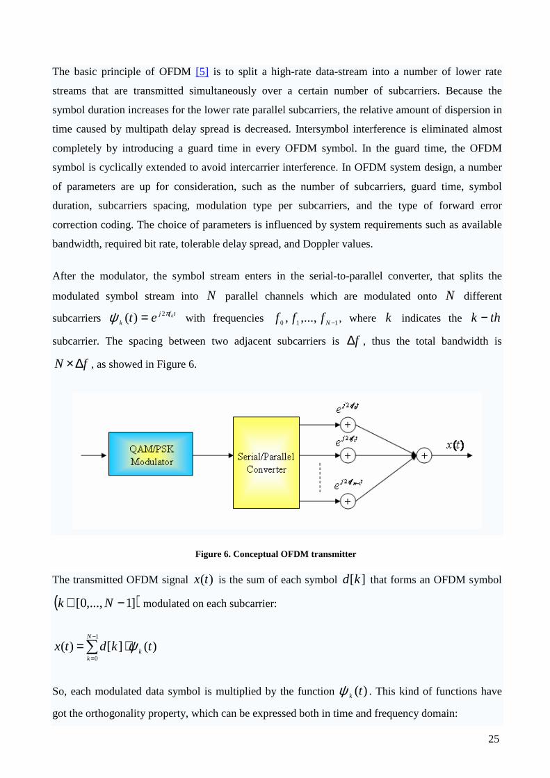
Each sub-carrier is modulated with a conventional modulation scheme (such as QAM/PSK, etc.) at a
low symbol rate, maintaining data rates similar to conventional single-carrier modulation schemes in
the same bandwidth, as showed in Figure 5.
Figure 5. Modulation of each sub-carrier
25
The basic principle of OFDM [5] is to split a high-rate data-stream into a number of lower rate
streams that are transmitted simultaneously over a certain number of subcarriers. Because the
symbol duration increases for the lower rate parallel subcarriers, the relative amount of dispersion in
time caused by multipath delay spread is decreased. Intersymbol interference is eliminated almost
completely by introducing a guard time in every OFDM symbol. In the guard time, the OFDM
symbol is cyclically extended to avoid intercarrier interference. In OFDM system design, a number
of parameters are up for consideration, such as the number of subcarriers, guard time, symbol
duration, subcarriers spacing, modulation type per subcarriers, and the type of forward error
correction coding. The choice of parameters is influenced by system requirements such as available
bandwidth, required bit rate, tolerable delay spread, and Doppler values.
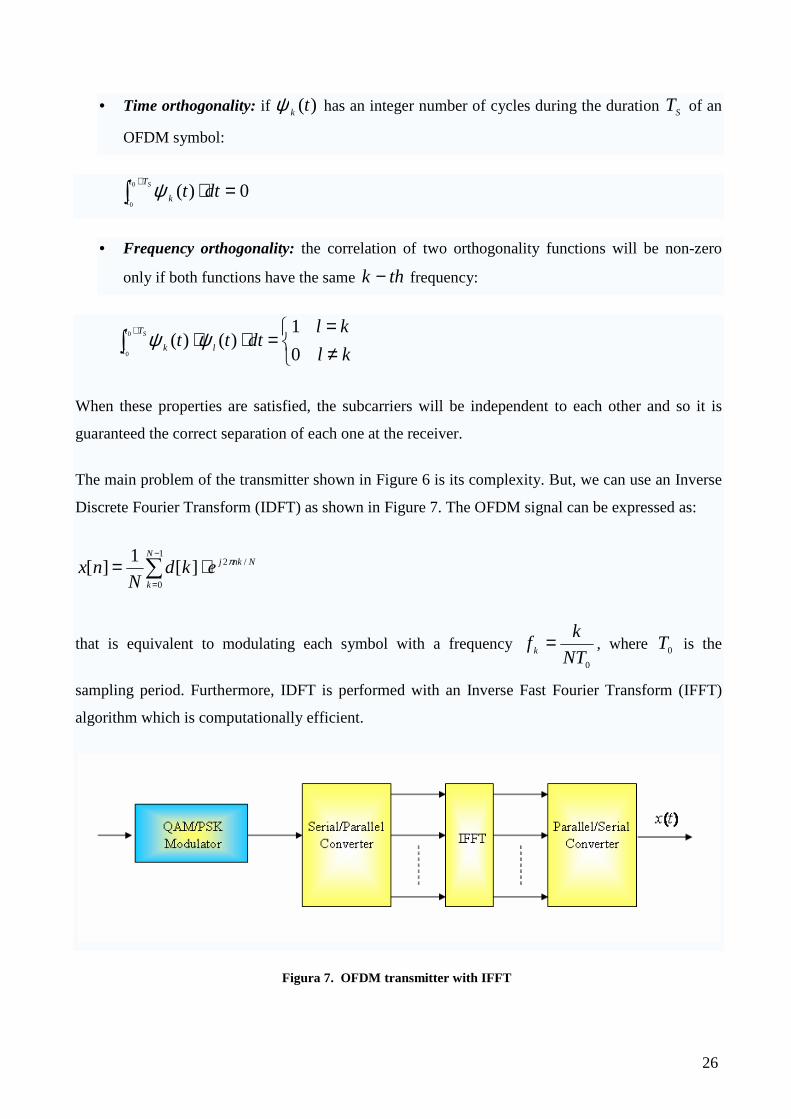
After the modulator, the symbol stream enters in the serial-to-parallel converter, that splits the
modulated symbol stream into N parallel channels which are modulated onto N different
subcarriers tfj
kket πψ 2)( = with frequencies 110 ,...,, −Nfff , where k indicates the thk −
subcarrier. The spacing between two adjacent subcarriers is f∆ , thus the total bandwidth is
fN ∆× , as showed in Figure 6.
Figure 6. Conceptual OFDM transmitter
The transmitted OFDM signal )(tx is the sum of each symbol ][kd that forms an OFDM symbol
( )]1,...,0[ −∈ Nk modulated on each subcarrier:
)(][)(1
0
tkdtx k
N
k
ψ⋅=∑−
=
So, each modulated data symbol is multiplied by the function )(tkψ . This kind of functions have
got the orthogonality property, which can be expressed both in time and frequency domain:
26
• Time orthogonality: if )(tkψ has an integer number of cycles during the duration ST of an
OFDM symbol:
0)(0
0
=⋅∫+ STt
t k dttψ
• Frequency orthogonality: the correlation of two orthogonality functions will be non-zero
only if both functions have the same thk − frequency:
≠=
=⋅⋅∫+
kl
kldtttSTt
t lk 0
1)()(0
0
ψψ
When these properties are satisfied, the subcarriers will be independent to each other and so it is
guaranteed the correct separation of each one at the receiver.
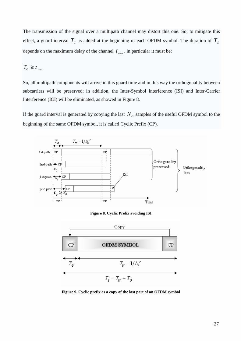
The main problem of the transmitter shown in Figure 6 is its complexity. But, we can use an Inverse
Discrete Fourier Transform (IDFT) as shown in Figure 7. The OFDM signal can be expressed as:
∑−
=⋅=
1
0
/2][1
][N
k
NnkjekdN
nx π
that is equivalent to modulating each symbol with a frequency 0NT
kf k = , where 0T is the
sampling period. Furthermore, IDFT is performed with an Inverse Fast Fourier Transform (IFFT)
algorithm which is computationally efficient.
Figura 7. OFDM transmitter with IFFT
27
The transmission of the signal over a multipath channel may distort this one. So, to mitigate this
effect, a guard interval GT is added at the beginning of each OFDM symbol. The duration of GT
depends on the maximum delay of the channel maxτ , in particular it must be:
maxτ≥GT
So, all multipath components will arrive in this guard time and in this way the orthogonality between
subcarriers will be preserved; in addition, the Inter-Symbol Interference (ISI) and Inter-Carrier
Interference (ICI) will be eliminated, as showed in Figure 8.
If the guard interval is generated by copying the last GN samples of the useful OFDM symbol to the
beginning of the same OFDM symbol, it is called Cyclic Prefix (CP).
Figure 8. Cyclic Prefix avoiding ISI
Figure 9. Cyclic prefix as a copy of the last part of an OFDM symbol
28
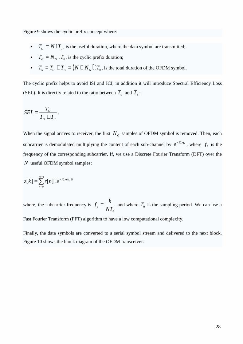
Figure 9 shows the cyclic prefix concept where:
• 0TNTU ⋅= , is the useful duration, where the data symbol are transmitted;
• 0TNT GG ⋅= , is the cyclic prefix duration;
• ( ) 0TNNTTT GGUS ⋅+=+= , is the total duration of the OFDM symbol.
The cyclic prefix helps to avoid ISI and ICI, in addition it will introduce Spectral Efficiency Loss
(SEL). It is directly related to the ratio between GT and ST :
UG
G
TT
TSEL
+= .
When the signal arrives to receiver, the first GN samples of OFDM symbol is removed. Then, each
subcarrier is demodulated multiplying the content of each sub-channel by kfje π2− , where kf is the
frequency of the corresponding subcarrier. If, we use a Discrete Fourier Transform (DFT) over the
N useful OFDM symbol samples:
∑−
=
−⋅=1
0
/2][][N
n
Nnkjenrkz π
where, the subcarrier frequency is 0NT
kf k = and where 0T is the sampling period. We can use a
Fast Fourier Transform (FFT) algorithm to have a low computational complexity.
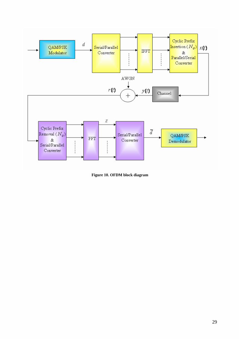
Finally, the data symbols are converted to a serial symbol stream and delivered to the next block.
Figure 10 shows the block diagram of the OFDM transceiver.
29
Figure 10. OFDM block diagram
30
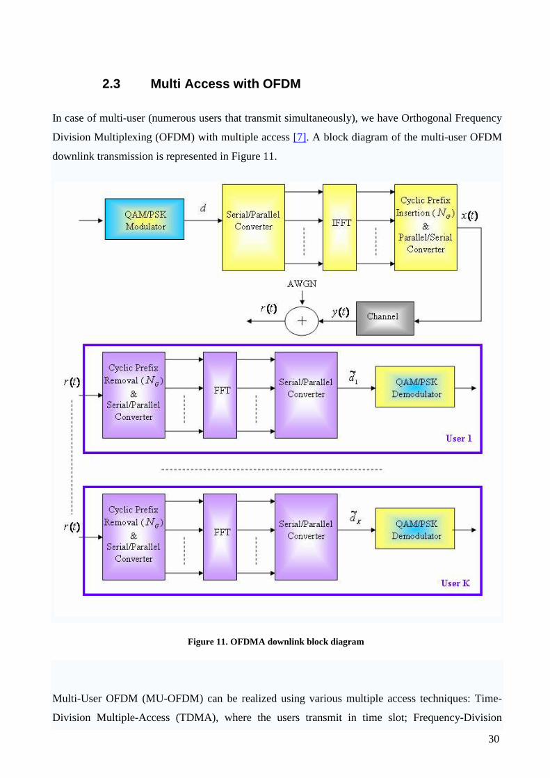
2.3 Multi Access with OFDM
In case of multi-user (numerous users that transmit simultaneously), we have Orthogonal Frequency
Division Multiplexing (OFDM) with multiple access [7]. A block diagram of the multi-user OFDM
downlink transmission is represented in Figure 11.
Figure 11. OFDMA downlink block diagram
Multi-User OFDM (MU-OFDM) can be realized using various multiple access techniques: Time-
Division Multiple-Access (TDMA), where the users transmit in time slot; Frequency-Division
31
Multiple-Access (FDMA), where the users transmit on a set of frequency ; Code-Division Multiple-
Access (CDMA), where the users transmit using a set of spreading sequences; or Space Division
Multiple-Access (SDMA), which reuses bandwidth by multiplexing signals based on their spatial
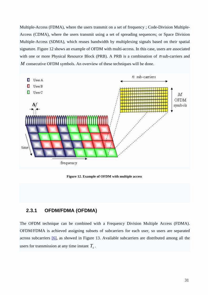
signature. Figure 12 shows an example of OFDM with multi-access. In this case, users are associated
with one or more Physical Resource Block (PRB). A PRB is a combination of nsub-carriers and
M consecutive OFDM symbols. An overview of these techniques will be done.
Figure 12. Example of OFDM with multiple access
2.3.1 OFDM/FDMA (OFDMA)
The OFDM technique can be combined with a Frequency Division Multiple Access (FDMA).
OFDM/FDMA is achieved assigning subsets of subcarriers for each user, so users are separated
across subcarriers [6], as showed in Figure 13. Available subcarriers are distributed among all the
users for transmission at any time instant ST .

32
Figure 13. MU-OFDM with FDMA
In OFDM/FDMA [7], the whole spectrum may be divided into multiple adjacent subcarriers. So, a
large number of userss share the whole spectrum. In base on the allocation of subcarriers to users,
we can have different kind of OFDM/FDMA: block FDMA (grouped carriers FDMA), random
allocation (adaptive frequency hopping) and interleaved FDMA (comb spread carriers), as showed
in Figure 14.
Figure 14. OFDM/FDMA variations
The OFDM/FDMA has significant interest because for its robustness to multipath propagation,
appropriateness for coverage extension and high spectral efficiency.
33
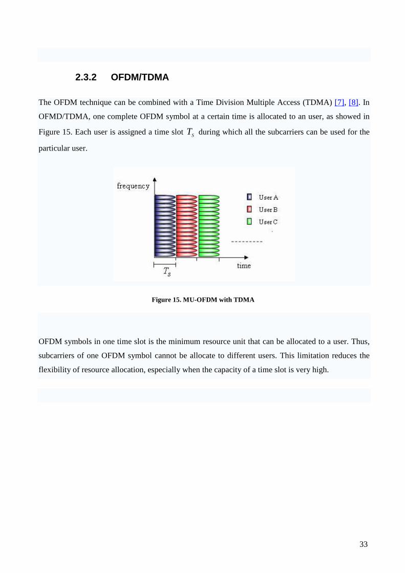
2.3.2 OFDM/TDMA
The OFDM technique can be combined with a Time Division Multiple Access (TDMA) [7], [8]. In
OFMD/TDMA, one complete OFDM symbol at a certain time is allocated to an user, as showed in
Figure 15. Each user is assigned a time slot ST during which all the subcarriers can be used for the
particular user.
Figure 15. MU-OFDM with TDMA
OFDM symbols in one time slot is the minimum resource unit that can be allocated to a user. Thus,
subcarriers of one OFDM symbol cannot be allocate to different users. This limitation reduces the
flexibility of resource allocation, especially when the capacity of a time slot is very high.
34
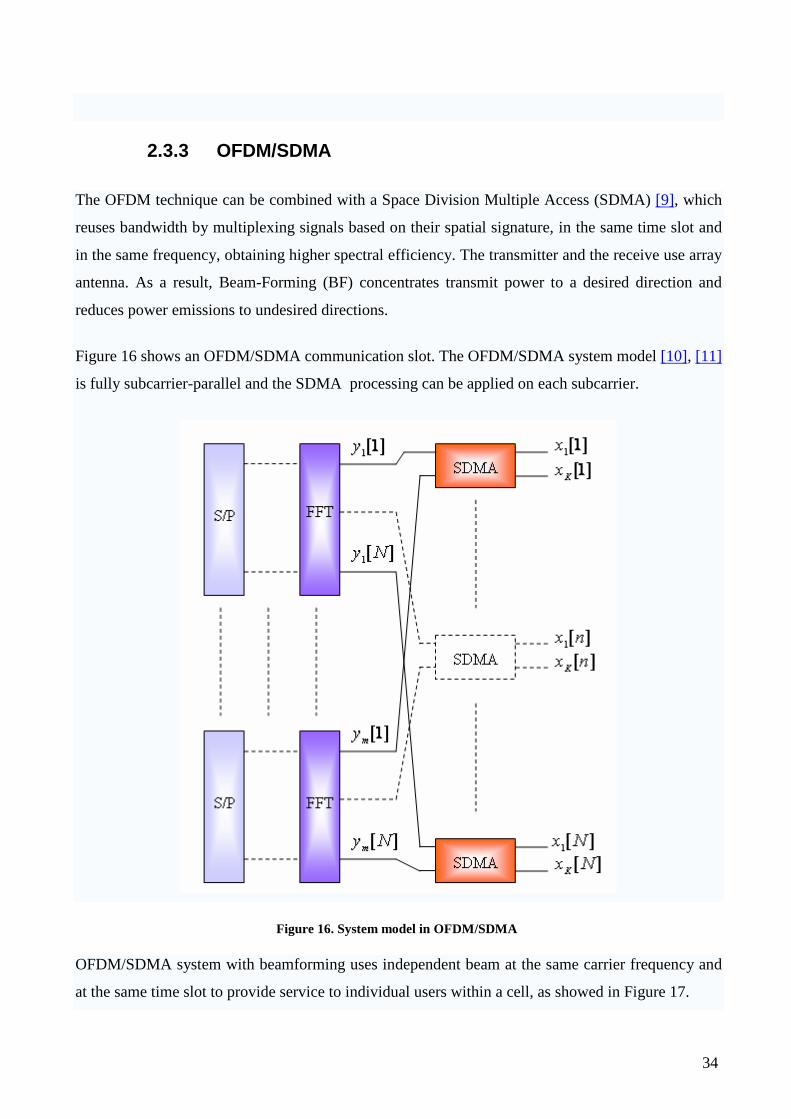
2.3.3 OFDM/SDMA
The OFDM technique can be combined with a Space Division Multiple Access (SDMA) [9], which
reuses bandwidth by multiplexing signals based on their spatial signature, in the same time slot and
in the same frequency, obtaining higher spectral efficiency. The transmitter and the receive use array
antenna. As a result, Beam-Forming (BF) concentrates transmit power to a desired direction and
reduces power emissions to undesired directions.
Figure 16 shows an OFDM/SDMA communication slot. The OFDM/SDMA system model [10], [11]
is fully subcarrier-parallel and the SDMA processing can be applied on each subcarrier.
Figure 16. System model in OFDM/SDMA
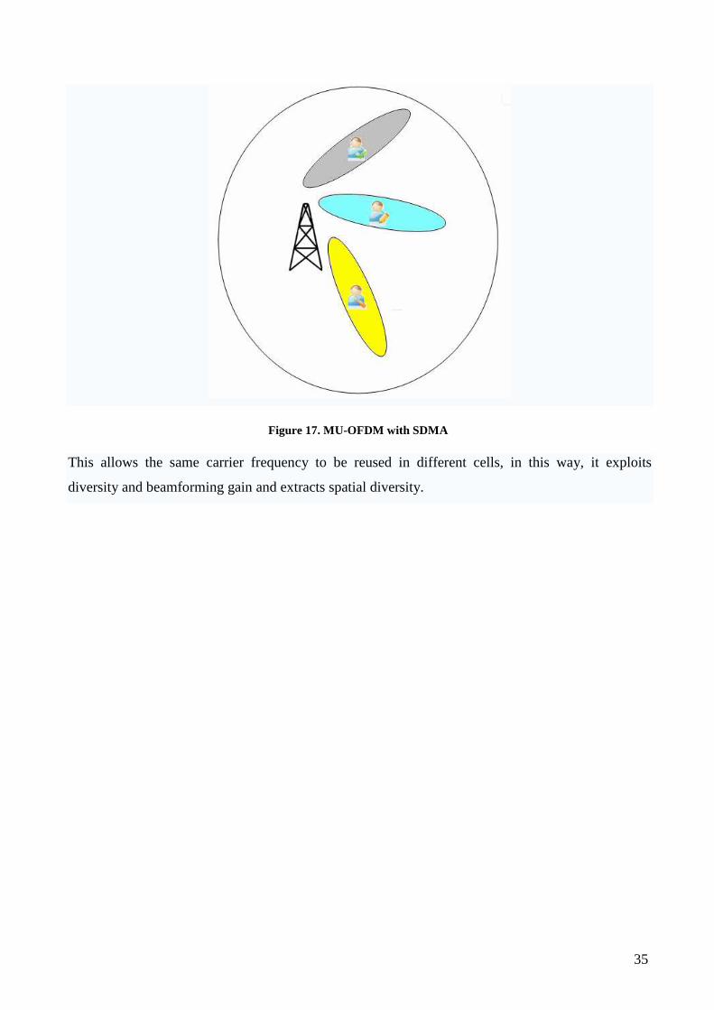
OFDM/SDMA system with beamforming uses independent beam at the same carrier frequency and
at the same time slot to provide service to individual users within a cell, as showed in Figure 17.
35
Figure 17. MU-OFDM with SDMA
This allows the same carrier frequency to be reused in different cells, in this way, it exploits
diversity and beamforming gain and extracts spatial diversity.

36
2.4 Beamforming
Beamforming (BF) [12] is a signal processing technique used with arrays of transmitting or
receiving transducers that control the directionality of, or sensitivity to, a radiation pattern. When
receiving a signal, beamforming can increase the receiver sensitivity in the direction of wanted
signals and decrease the sensitivity in the direction of interference and noise. When transmitting a
signal, beamforming can increase the power in the direction the signal is to be sent. The change
compared with an omnidirectional receiving pattern is known as the receive gain (or loss). The
change compared with an omnidirectional transmission is known as the transmission gain. These
changes are done by creating beams and nulls in the radiation pattern. Figure 18 illustrates the polar
diagram of the antenna array.
Figure 18. Polar diagram of a typical antenna beampattern.
Beamforming is a mix between antenna technology and digital technology [13]. An antenna can be
considered to be a device that converters spatial-temporal signals, thus making them available to a a
wide variety of signal processing techniques, in this way, all of the desired information that is being
carried by these signals can be extracted. Figure 19 shows a generic BF antenna system.

37
Figure 19. A generic BF antenna system
Antenna arrays using adaptive beamforming techniques can reject interfering signals having a
Direction Of Arrival (DOA) different from that of a desired signal [13]. An adaptive BF is a device
that is able to separate signals collocated in the frequency band but separated in the spatial domain.
This provides a means for separating a desired signal from interfering signals. An adaptive BF is
able to automatically optimize the array pattern by adjusting the elemental control weights until a
prescribed objective function is satisfied. If a wave (for example a plane wave) arrive perpendicular
to the array, it is seen with the same phase from all transducers; so the sum of the array output
signals is just wave incident. Instead, if the arrival angle is different from 90°, the array output is
attenuated regarding the previous one, and it depends on angle incident, as showed in Figure 20.
Figure 20. Signal output array [13]
38
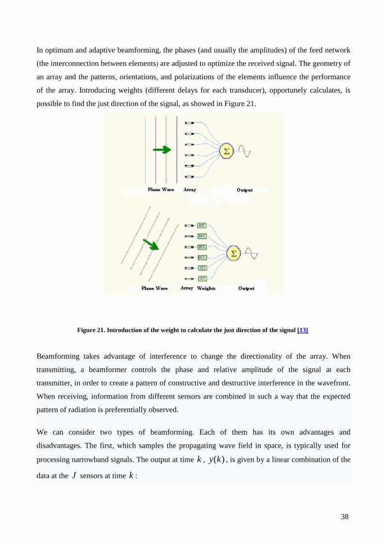
In optimum and adaptive beamforming, the phases (and usually the amplitudes) of the feed network
(the interconnection between elements) are adjusted to optimize the received signal. The geometry of
an array and the patterns, orientations, and polarizations of the elements influence the performance
of the array. Introducing weights (different delays for each transducer), opportunely calculates, is
possible to find the just direction of the signal, as showed in Figure 21.
Figure 21. Introduction of the weight to calculate the just direction of the signal [13]
Beamforming takes advantage of interference to change the directionality of the array. When
transmitting, a beamformer controls the phase and relative amplitude of the signal at each
transmitter, in order to create a pattern of constructive and destructive interference in the wavefront.
When receiving, information from different sensors are combined in such a way that the expected
pattern of radiation is preferentially observed.
We can consider two types of beamforming. Each of them has its own advantages and
disadvantages. The first, which samples the propagating wave field in space, is typically used for
processing narrowband signals. The output at time k , )(ky , is given by a linear combination of the
data at the J sensors at time k :
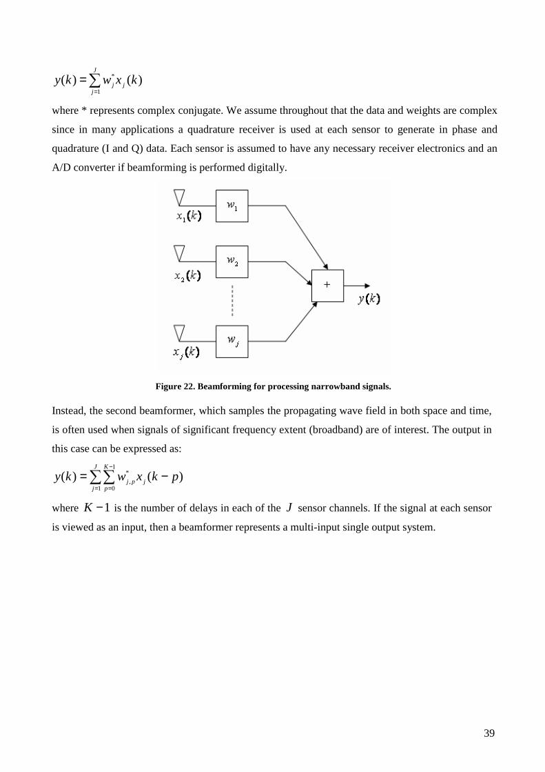
39
∑=
=J
jjj kxwky
1
* )()(
where * represents complex conjugate. We assume throughout that the data and weights are complex
since in many applications a quadrature receiver is used at each sensor to generate in phase and
quadrature (I and Q) data. Each sensor is assumed to have any necessary receiver electronics and an
A/D converter if beamforming is performed digitally.
Figure 22. Beamforming for processing narrowband signals.
Instead, the second beamformer, which samples the propagating wave field in both space and time,
is often used when signals of significant frequency extent (broadband) are of interest. The output in
this case can be expressed as:
∑∑=
−
=−=
J
j
K
pjpj pkxwky
1
1
0
*, )()(
where 1−K is the number of delays in each of the J sensor channels. If the signal at each sensor
is viewed as an input, then a beamformer represents a multi-input single output system.

40
Figure 23. Beamforming for processing broadband signals.
It is convenient to develop notation which permits us to treat both beamformers in Figure 22 and
Figure 23 simultaneously, so we can obtain:
)()( kxwky H=
by appropriately defining a weight vector w and data vector )(kx .
Beamforming is sometimes performed in the frequency domain when broadband signals are of
interest. Figure 24 illustrates transformation of the data at each sensor into the frequency domain.
Weighted combinations of the data at each frequency (bin) are formed. An inverse discrete Fourier
transform produces the output time series:
Figure 24. Beamforming performed in the frequency domain for the broadband signals
41
Beamformer can be classified as either data independent or statistically optimum, depending on how
the weights are chosen. The weights in a data independent beamformer do not depend on the array
data and are chosen to present a specified response for all signal/interference scenarios. The weights
in a statistically optimum beamformer are chosen based on the statistics of the array data to optimize
the array response. In the receive BF (uplink case), the main objective is to maximize the Signal
Noise Rate (SNR) of the received desired signal. In the transmit BF (downlink case), the objective
remains the same, even if the means to obtain it may be different. In fact, is possible to maximize the
power in the direction of user, that must receive the signal, and minimize the interference to another
users, maximizing the downlink SNR. If the transfer function of the channel is known at the
transmitter, the downlink SNR can be maximized by multiplying the desired signal with a set of
weights [13]. It can be shown that the weights are a scale version of the uplink weights, that we saw
before.
42
2.4.1 Beamforming-Based SDMA
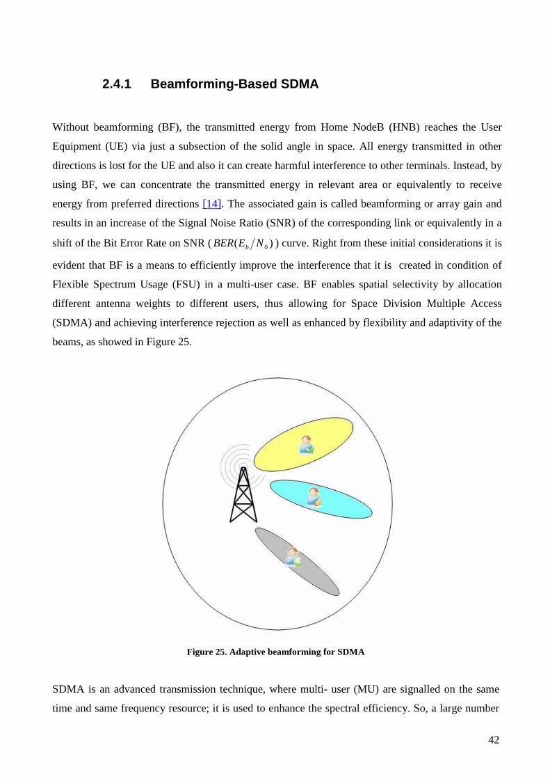
Without beamforming (BF), the transmitted energy from Home NodeB (HNB) reaches the User
Equipment (UE) via just a subsection of the solid angle in space. All energy transmitted in other
directions is lost for the UE and also it can create harmful interference to other terminals. Instead, by
using BF, we can concentrate the transmitted energy in relevant area or equivalently to receive
energy from preferred directions [14]. The associated gain is called beamforming or array gain and
results in an increase of the Signal Noise Ratio (SNR) of the corresponding link or equivalently in a
shift of the Bit Error Rate on SNR ( )( 0NEBER b ) curve. Right from these initial considerations it is
evident that BF is a means to efficiently improve the interference that it is created in condition of
Flexible Spectrum Usage (FSU) in a multi-user case. BF enables spatial selectivity by allocation
different antenna weights to different users, thus allowing for Space Division Multiple Access
(SDMA) and achieving interference rejection as well as enhanced by flexibility and adaptivity of the
beams, as showed in Figure 25.
Figure 25. Adaptive beamforming for SDMA
SDMA is an advanced transmission technique, where multi- user (MU) are signalled on the same
time and same frequency resource; it is used to enhance the spectral efficiency. So, a large number

43
of User Equipments (UEs) share the whole spectrum. In this scheme HNB prepares a number of
directional beams to cover the UEs area. BF concentrates transmit power to a desired direction and
reduces power emissions to undesired directions; this way BF eliminate Multi-User Interference
(MUI) caused by all others UEs. Another advantages of beamforming techniques are low cost of the
UE, high directivity.
44
2.5 MIMO System
Multiple Input Multiple Output (MIMO) system uses multiple antennas at both the transmitter and
receiver to improve communication performance [15], [16]. The research in this field has started
approximately 15 years ago about, but it rapidly progressed, attracting attention in wireless
communication, because it allows to increase throughput and link range without additional
bandwidth or transmit power, in add it is immune to fading, interference and noise.
MIMO to achieve high spectral efficiency and a very wide spectrum allocation in the range of
MHz100 . In MIMO communications systems, multiple antenna are used at both sides of the link.
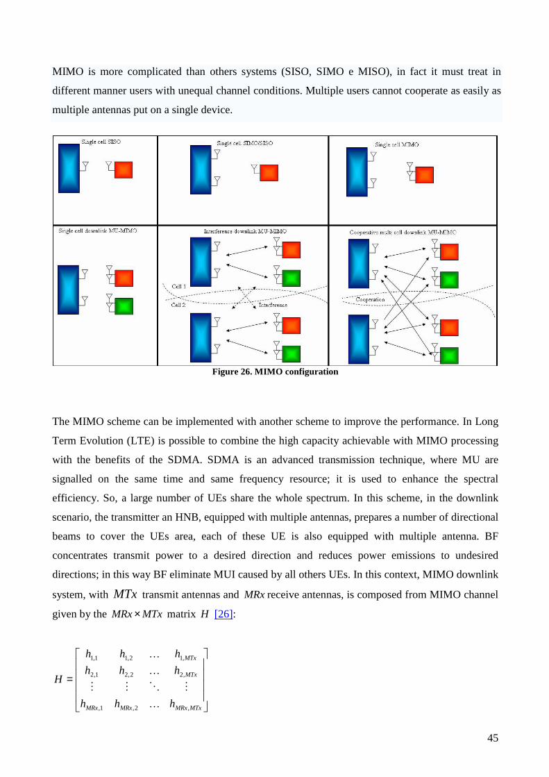
Figure 26 shows the different kinds of MIMO configurations [17]. Where:
• SISO: Single Input Single Output, one antenna at the transmitter and one at the receiver;
• SIMO: Single Input Multiple Output, one antenna at the transmitter and many at the
receiver;
• MISO: Multiple Input Single Output, many antenna at the transmitter and one at the
receiver;
• MIMO: Multiple Input Multiple Output, many antenna at the transmitter and many at the
receiver.
In a digital communication system, the fundamental performance parameters are the Bit Error Rate
(BER) and the number of bits that we are able to send through the channel, per units of time and
frequency (Throughput, measured in bit/s/Hz), guaranteeing an arbitrarily low error probability.
With SISO, SIMO and MISO to obtain the same advantages, it is necessary to use more power and
more bandwidth compared to the MIMO case. MIMO introduces two main gains:
• Multiplexing gain: different signals sent through different parallel channels, leading to the
information transmission rate increase;
• Diversity gain: the same signals sent through different parallel channels, leading to the BER
improvement.
45
MIMO is more complicated than others systems (SISO, SIMO e MISO), in fact it must treat in
different manner users with unequal channel conditions. Multiple users cannot cooperate as easily as
multiple antennas put on a single device.
Figure 26. MIMO configuration
The MIMO scheme can be implemented with another scheme to improve the performance. In Long
Term Evolution (LTE) is possible to combine the high capacity achievable with MIMO processing
with the benefits of the SDMA. SDMA is an advanced transmission technique, where MU are
signalled on the same time and same frequency resource; it is used to enhance the spectral
efficiency. So, a large number of UEs share the whole spectrum. In this scheme, in the downlink
scenario, the transmitter an HNB, equipped with multiple antennas, prepares a number of directional
beams to cover the UEs area, each of these UE is also equipped with multiple antenna. BF
concentrates transmit power to a desired direction and reduces power emissions to undesired
directions; in this way BF eliminate MUI caused by all others UEs. In this context, MIMO downlink
system, with MTx transmit antennas and MRxreceive antennas, is composed from MIMO channel
given by the MTxMRx× matrix H [26]:
=
MTxMRxMRxMRx
MTx
MTx
hhh
hhh
hhh
H
,2,1,
,22,21,2
,12,11,1
K
MOMM
K
K
46
where jih , is the channel impulse response between the thj − ( MTxj ,...,2,1= ) transmit antenna
and the thi − ( MRxi ,...,2,1= ) receive antenna.

47
48
Chapter 3
3. Project description
This project considers a beamforming and power control algorithm for MU downlink MIMO-
OFDM systems, in a LA scenario, with LTE1 [24], [25]. advanced systems in the FSU context [28],
[29].
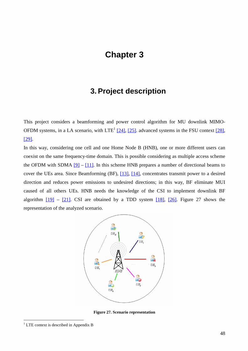
In this way, considering one cell and one Home Node B (HNB), one or more different users can
coexist on the same frequency-time domain. This is possible considering as multiple access scheme
the OFDM with SDMA [9] – [11]. In this scheme HNB prepares a number of directional beams to
cover the UEs area. Since Beamforming (BF), [13], [14], concentrates transmit power to a desired
direction and reduces power emissions to undesired directions; in this way, BF eliminate MUI
caused of all others UEs. HNB needs the knowledge of the CSI to implement downlink BF
algorithm [19] – [21]. CSI are obtained by a TDD system [18], [26]. Figure 27 shows the
representation of the analyzed scenario.
Figure 27. Scenario representation
1 LTE context is described in Appendix B
49
3.1 Scenario
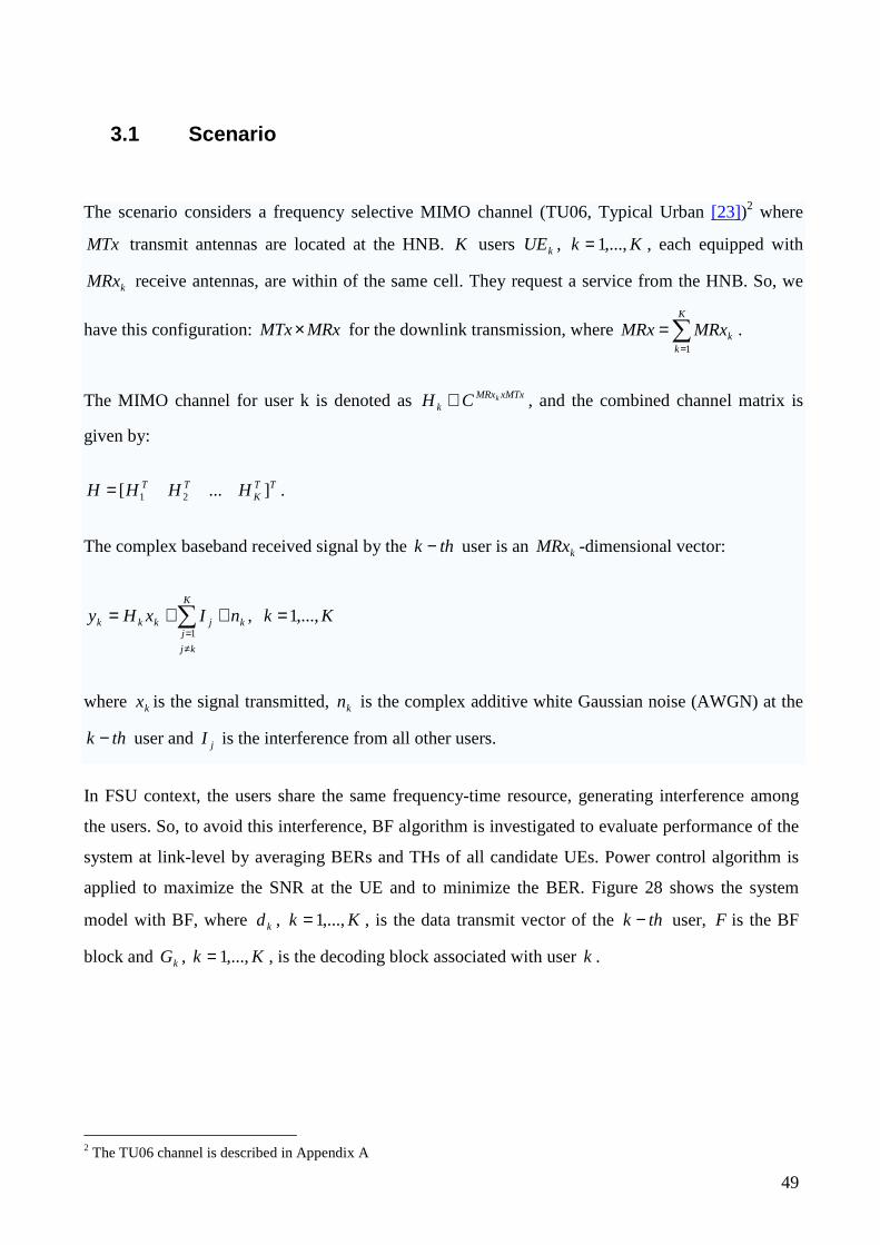
The scenario considers a frequency selective MIMO channel (TU06, Typical Urban [23])2 where
MTx transmit antennas are located at the HNB. K users kUE , Kk ,...,1= , each equipped with
kMRx receive antennas, are within of the same cell. They request a service from the HNB. So, we
have this configuration: MRxMTx× for the downlink transmission, where ∑=
=K
kkMRxMRx
1
.
The MIMO channel for user k is denoted as xMTxMRxk
kCH ∈ , and the combined channel matrix is
given by:
TTK
TT HHHH ]...[ 21= .
The complex baseband received signal by the thk − user is an kMRx -dimensional vector:
KknIxHy k
K
kj
jjkkk ,...,1,
1
=++= ∑≠=
where kx is the signal transmitted, kn is the complex additive white Gaussian noise (AWGN) at the
thk − user and jI is the interference from all other users.
In FSU context, the users share the same frequency-time resource, generating interference among
the users. So, to avoid this interference, BF algorithm is investigated to evaluate performance of the
system at link-level by averaging BERs and THs of all candidate UEs. Power control algorithm is
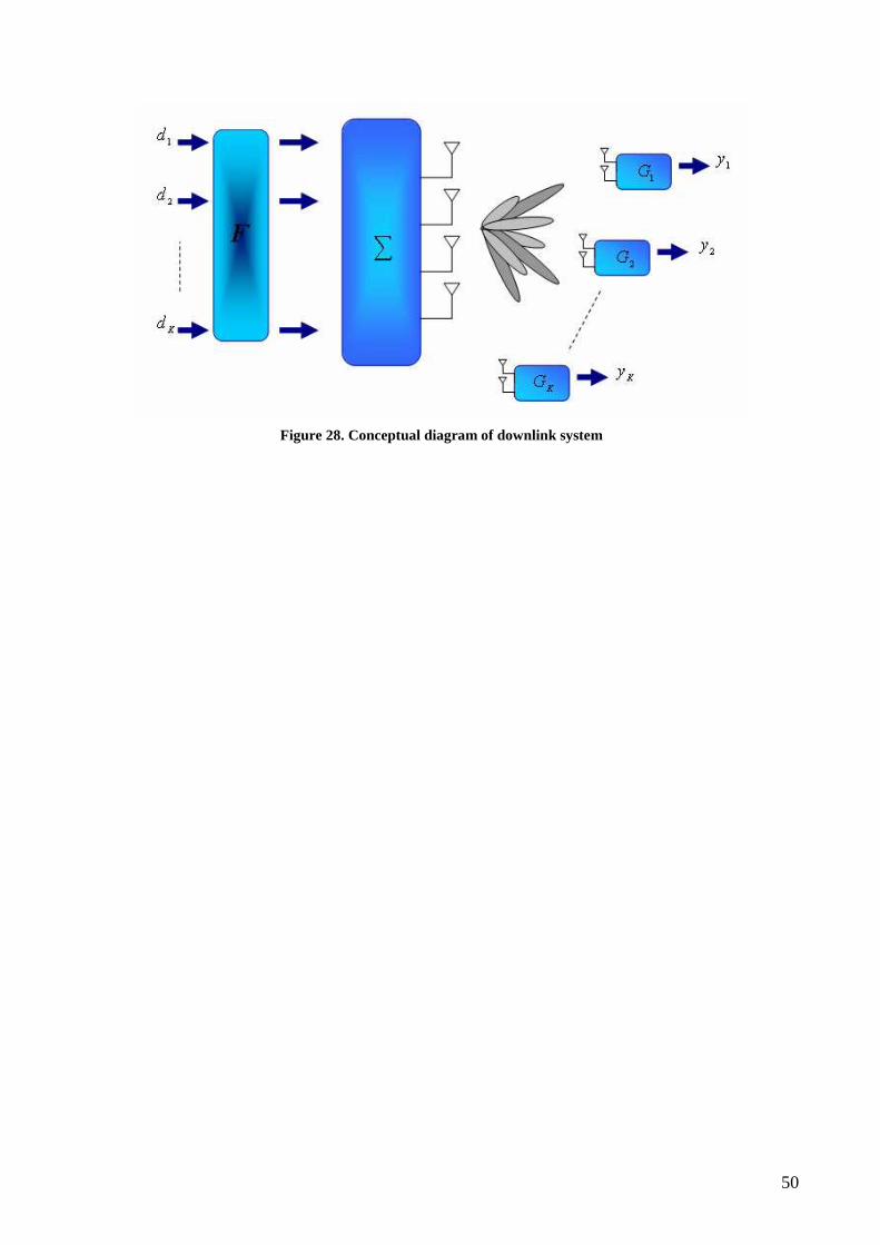
applied to maximize the SNR at the UE and to minimize the BER. Figure 28 shows the system
model with BF, where kd , Kk ,...,1= , is the data transmit vector of the thk − user, F is the BF
block and kG , Kk ,...,1= , is the decoding block associated with user k .
2 The TU06 channel is described in Appendix A
50
Figure 28. Conceptual diagram of downlink system
51
3.2 System Architecture for LTE
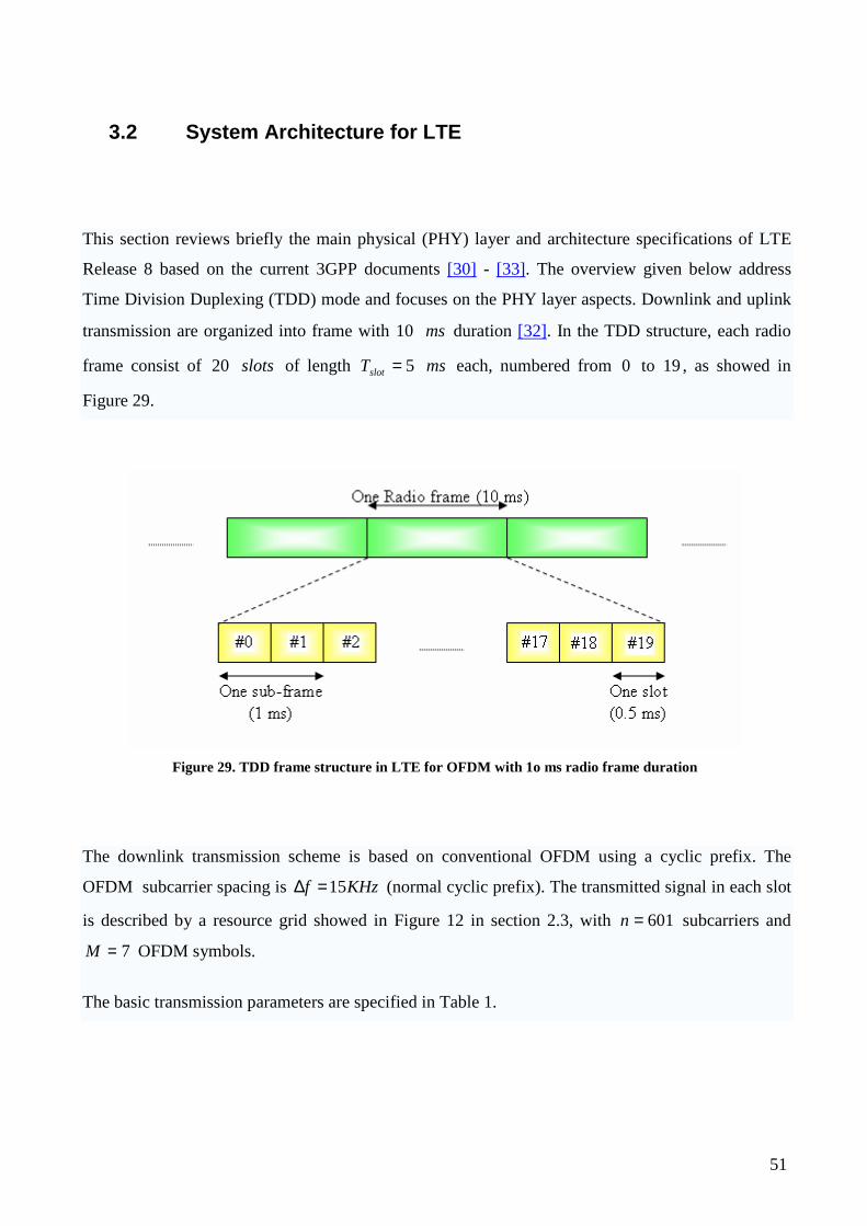
This section reviews briefly the main physical (PHY) layer and architecture specifications of LTE
Release 8 based on the current 3GPP documents [30] - [33]. The overview given below address
Time Division Duplexing (TDD) mode and focuses on the PHY layer aspects. Downlink and uplink
transmission are organized into frame with ms10 duration [32]. In the TDD structure, each radio
frame consist of slots20 of length msTslot 5= each, numbered from 0 to 19 , as showed in
Figure 29.
Figure 29. TDD frame structure in LTE for OFDM with 1o ms radio frame duration
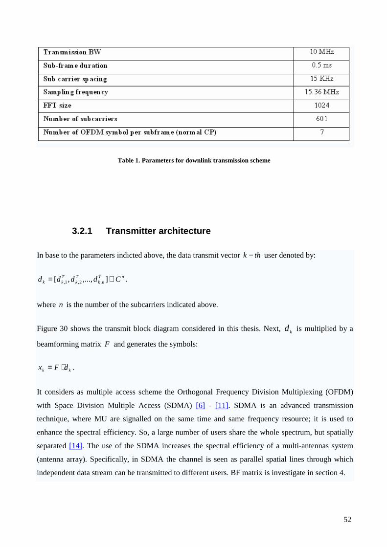
The downlink transmission scheme is based on conventional OFDM using a cyclic prefix. The
OFDM subcarrier spacing is KHzf 15=∆ (normal cyclic prefix). The transmitted signal in each slot
is described by a resource grid showed in Figure 12 in section 2.3, with 601=n subcarriers and
7=M OFDM symbols.
The basic transmission parameters are specified in Table 1.
52
Table 1. Parameters for downlink transmission scheme
3.2.1 Transmitter architecture
In base to the parameters indicted above, the data transmit vector thk − user denoted by:
nTnk
Tk
Tkk Cdddd ∈= ],...,,[ ,2,1, .
where n is the number of the subcarriers indicated above.
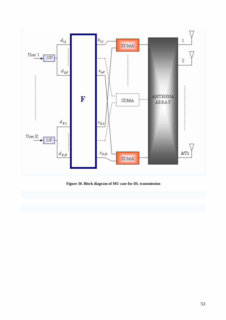
Figure 30 shows the transmit block diagram considered in this thesis. Next, kd is multiplied by a
beamforming matrix F and generates the symbols:
kk dFx ⋅= .
It considers as multiple access scheme the Orthogonal Frequency Division Multiplexing (OFDM)
with Space Division Multiple Access (SDMA) [6] - [11]. SDMA is an advanced transmission
technique, where MU are signalled on the same time and same frequency resource; it is used to
enhance the spectral efficiency. So, a large number of users share the whole spectrum, but spatially
separated [14]. The use of the SDMA increases the spectral efficiency of a multi-antennas system
(antenna array). Specifically, in SDMA the channel is seen as parallel spatial lines through which
independent data stream can be transmitted to different users. BF matrix is investigate in section 4.
53
Figure 30. Block diagram of MU case for DL transmission
54
3.2.2 Channel model
The structure of the MIMO channel MTxMRxCH ×∈ [26] depends on the number of transmit and
receive antennas and the combined channel matrix is given by:
TT
K
TT HHHH ]...[ 21= .
where MTxMRxk
kCH ×∈ denoted the matrix channel of the thk − user and is define as:
=),()1,(
),1()1,1(
MTxMRx
k
MRx
k
MTx
kk
k
kk hh
hh
H
K
MOM
K
where ),( ji
kh represents the channel coefficient from the thj − transmit antenna at the HNB to the
thi − receiver antenna at thk − user.
We assume that the channel transfer matrix H is perfectly know to the HNB, through reverse
channel estimation in TDD. In fact, in TDD system, using the reciprocity principle3 it is possible to
use the estimated uplink channel for downlink transmission. In a TDD system, the uplink and
downlink transmissions share the same frequency but are using different time slots. If the delay
between these two slots is short compared to the coherence time of the channel, the spatial signature
of the downlink and uplink will be the same. This means that the instantaneous uplink channel can
be used as a good estimate of the downlink channel. But, if the delay between the two slots is longer
than the coherence time, this method cannot be used.
So, perfect CSI is assumed at the HNB. It is also assumed that kH is perfectly known at the thk −
user , but other users’ channels are not known by thk − user.
3 The reciprocity principle is described in TDD system in Appendix C.
55
3.2.3 Receive architecture
At the receiver [18], the received signal vector at the thk − user, with Kk ,...,1= is defined as:
kkkkkkk ndFHnxHy +⋅⋅=+⋅=
where kH is the channel matrix of the thk − user , F is the beamforming matrix, kd is the
transmitted data signal vector at the thk − user and kn is the AWGN vector at the thk − user. The
thk − receiver knows à priori the beamforming matrix F and treats the combination FH k as an
effective channel. It detects and decodes the received signal to obtain an estimate of the transmitted
data signal vector kd . Considering decoding matrix kG and the received signal at thk − will be:
k
K
kkkkkk ndFHGyG +⋅⋅⋅=⋅ ∑
=1
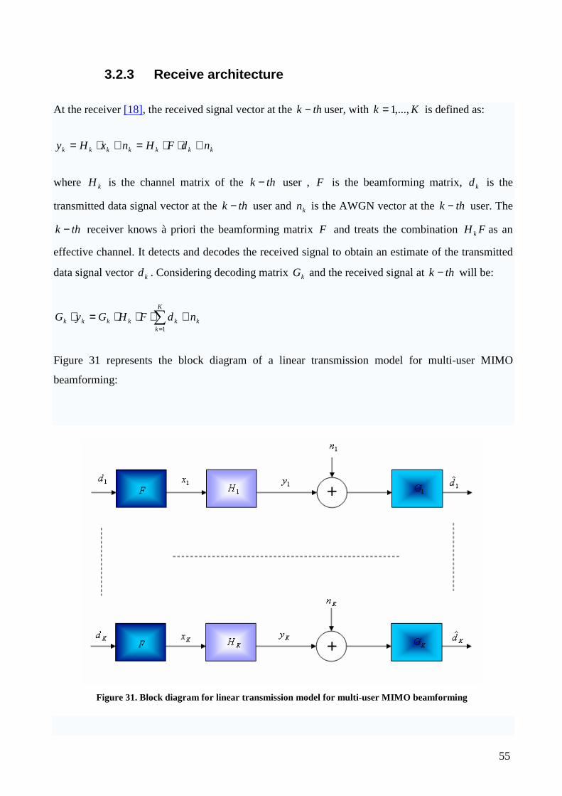
Figure 31 represents the block diagram of a linear transmission model for multi-user MIMO
beamforming:
Figure 31. Block diagram for linear transmission model for multi-user MIMO beamforming

56
The receiver can use one out of several detection methods, depending on the performance and
complexity requirements. In this thesis, we use the linear MMSE, where kG is designed according to
[18]:
( ) 22ˆminFkkkk
FGnGdIFHGEddE
k
+−=−
And the optimum MMSE receiver for the thk − user is given as:
( ) Hk
Hk
Hk
Hnk HFFHHFIG
k
12 −+= σ
where 2
knσ is the noise power of the thk − user.

57
58
Chapter 4
4. Beamforming methods
Beamforming techniques can be classified according to the amount of the MUI that is suppressed at
the transmitter and according to linearity. The linear beamforming matrix F can be modelled in sub-
matrices, each submatricex corresponding to one user:
[ ]KFFFF ...21=
where nMTxk CF ×∈ is the sub-matrix corresponds to thk − user, MTx is the number of transmitted
antenna and n is the number of subcarriers.
The beamforming matrix is a function of the CSIT. When we have perfect CSIT, the MIMO channel
can be decomposed into independent and parallel additive white noise channels, so the elements of
kH are complex Gaussian variables with zero-mean and unit-variance. These parallel channels are
defined by performing the Singular Value Decomposition (SVD) of the channel matrix as:
HHHH VUH Σ= .
where the lower H means the matrix is referred to the channel and the upper one indicates the
hermitian operator. The channel matrix H is a complex matrix of dimension MTxMRx× , so HU is
an MRxMRx× square unitary matrix, that is, IUUUU HHHH
HH == ; HΣ is MTxMRx× matrix
with nonnegative real numbers on the diagonal and zeros off the diagonal; and HHV denotes the
hermitian of HV and it is an MTxMTx× square unitary square matrix, i.e. IVVVV HHHH
HH == .
The parallel channels can be processed independently, each with independent modulation and
coding.

59
Also the beamforming matrix can be decompose by SVD:
HFFF VUF Σ=
where the left singular vectors FU represent the orthogonal beam direction; the squared singular
matrix 2FΣ are associated with the beam power loading; and the right singular vectors FV form the
input shaping matrix.
The optimal beam directions with perfect CSIT for all methods, can be obtained by:
HF VU =
According to the receive model treated above, the optimal beam directions are given by the
eigenvectors of HH H .
In this thesis are treated two different methods to calculate the beamforming matrix: Zero -Forcing
(Z-F) Beamforming and Successive Minimum Mean Square Error (SMMSE) Beamforming.
60
4.1 Zero-Forcing (ZF)
Zero-Forcing (ZF) [14], [19], [20] is a generalization of channel inversion when we have multiple
antennas per user. ZF BF algorithm is discussed in details in [19]. The fundamental idea is to select
the BF matrix jF at the thj − receive antenna, with MRxj ,...,1= .
The signal at thj − receive antenna, MRxj ,...,1= , can be rewritten as:
jjjjiij
K
ijiijj ndFHdFHndFHy ++=+=∑
=
~~
1
where, with Kk ,...1= users:
[ ][ ]T
KTj
Tj
TTj
Kjjj
ddddd
FFFFF
......~
......~
111
111
+−
+−
=
=
The optimal solution under the constraint that all MUI be zero (Zero-Forcing) is that HF is block
diagonal. So, to eliminate all MUI, we impose the constraint (Zero-Forcing) that:
0~ =jj FH
Defining jH~
as:
[ ]TK
Tj
Tj
Tj HHHHH ......
~111 +−=
It cans be decomposed using SVD:
[ ]HjjjjH
jjjj VVUVUH )0()1( ~~~~~~~~∑=∑=
where )1(~jV contains the first jL
~ right singular vectors, and )0(~
jV contains the last ( )jLNTx~− right
singular vectors, where )~
(~
jj HrankL = .
Defining the matrix:
61
=′
)0(
)0(22
)0(11
~...00
.........
0...~
0
0...0~
KKVH
VH
VH
HO
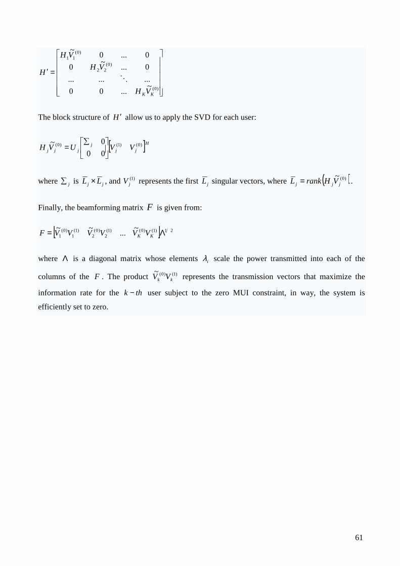
The block structure of H ′ allow us to apply the SVD for each user:
[ ]H
jjj
jjj VVUVH )0()1()0(
00
0~
∑=
where j∑ is jj LL × , and )1(jV represents the first jL singular vectors, where ( ))0(~
jjj VHrankL = .
Finally, the beamforming matrix F is given from:
[ ] 21)1()0()1(2
)0(2
)1(1
)0(1
~...
~~ Λ= KK VVVVVVF
where Λ is a diagonal matrix whose elements iλ scale the power transmitted into each of the
columns of the F . The product )1()0(~kk VV represents the transmission vectors that maximize the
information rate for the thk − user subject to the zero MUI constraint, in way, the system is
efficiently set to zero.
62
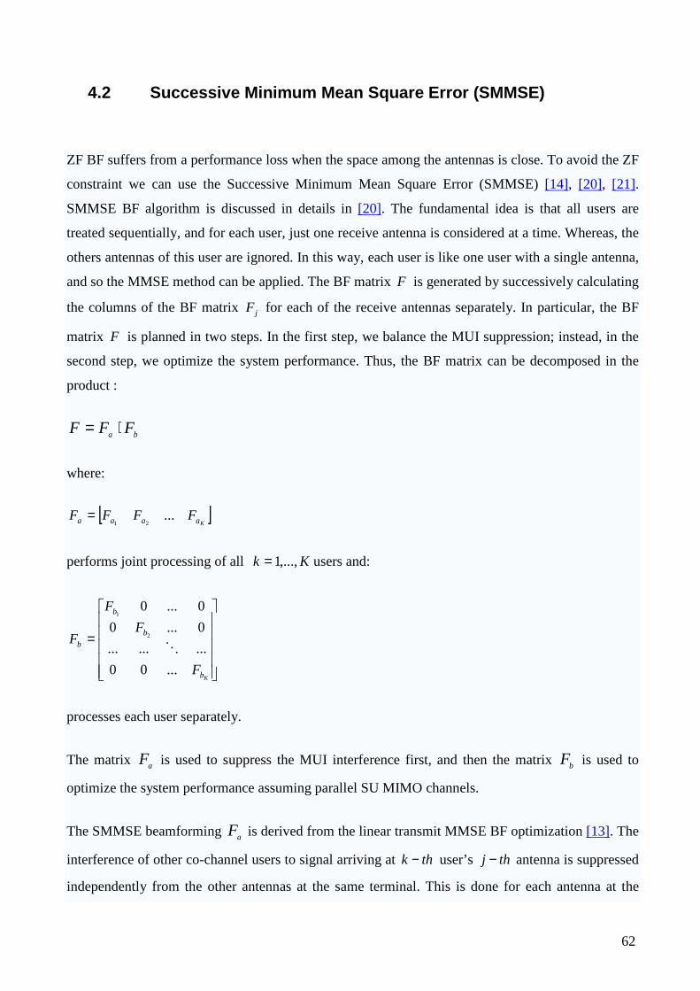
4.2 Successive Minimum Mean Square Error (SMMSE)
ZF BF suffers from a performance loss when the space among the antennas is close. To avoid the ZF
constraint we can use the Successive Minimum Mean Square Error (SMMSE) [14], [20], [21].
SMMSE BF algorithm is discussed in details in [20]. The fundamental idea is that all users are
treated sequentially, and for each user, just one receive antenna is considered at a time. Whereas, the
others antennas of this user are ignored. In this way, each user is like one user with a single antenna,
and so the MMSE method can be applied. The BF matrix F is generated by successively calculating
the columns of the BF matrix jF for each of the receive antennas separately. In particular, the BF
matrix F is planned in two steps. In the first step, we balance the MUI suppression; instead, in the
second step, we optimize the system performance. Thus, the BF matrix can be decomposed in the
product :
ba FFF ⋅=
where:
[ ]Kaaaa FFFF ...
21=
performs joint processing of all Kk ,...,1= users and:
=
Kb
b
b
b
F
F
F
F
...00
.........
0...0
0...0
2
1
O
processes each user separately.
The matrix aF is used to suppress the MUI interference first, and then the matrix bF is used to
optimize the system performance assuming parallel SU MIMO channels.
The SMMSE beamforming aF is derived from the linear transmit MMSE BF optimization [13]. The
interference of other co-channel users to signal arriving at thk − user’s thj − antenna is suppressed
independently from the other antennas at the same terminal. This is done for each antenna at the

63
same user terminal successively. So, the columns in the precoding matrix iaF , each corresponding to
one receive antenna, are calculated successively. Thus, the thj − column of the thk − user’s
precoding matrix iaF , corresponding to the thk − user’s thj − receive antenna, is equal to the first
column of the matrix jiaF
, which is obtained from the following equation:
( ) 1
,,,,
−×⋅+= MTxMTx
Hjkjk
Hjka IHHHF
jkα
where kMRxj ,...,1= is the thj − receive antenna of the thk − user, with Kk ,...,1= . Instead, jkH ,
is defined as:
MTxMRxMRx
K
k
k
Tjk
jkkC
H
H
H
H
h
H ×+−
+
− ∈
= )1(
1
1
1
,
,
...
...
where Tjkh , is the thj − row of the thk − user’s channel matrix kH .The first column of
jkaF,
is then
used as thj − column of kaF . After all columns of aF have been determined in this way. The
parameter α is chosen in accord with the transmit power and it is defined as:
tr
jknn
P
Rtr )( ,,=α
where trP is the average power of the transmit vector dFx ⋅= , that is:
{ } trH PFFtrxE == )(
2.
Instead, jknnR ,, define the corresponding receive noise covariance matrix. It is a diagonal matrix,
having the noise power of the thk − user at thj − receive antenna as element of the diagonal.
After calculating the BF vectors for all receive antennas in this way, the equivalent combined matrix
of all users is equal to MRxMRxa CHF ×∈ after the BF. For high SNR, this matrix is also block

64
diagonal, so we can decompose this matrix by SVD for each user. In fact, kak FH , represents the
resulting single-user MIMO channel of the thk − user:
Hkkkk
Hkkkkak VVUVUFH ][ )0()1(
, Σ=Σ=
So, we obtain that kbF , is the right column vectors of kV :
)0(
, kkb VF =
and then:
=
Kb
b
b
b
F
F
F
F
...00
.........
0...0
0...0
2
1
O
Finally, the beamforming matrix F is given from:
Λ⋅⋅= ba FFF
where Λ is a diagonal power loading matrix, analogous to the one for ZF method.
65
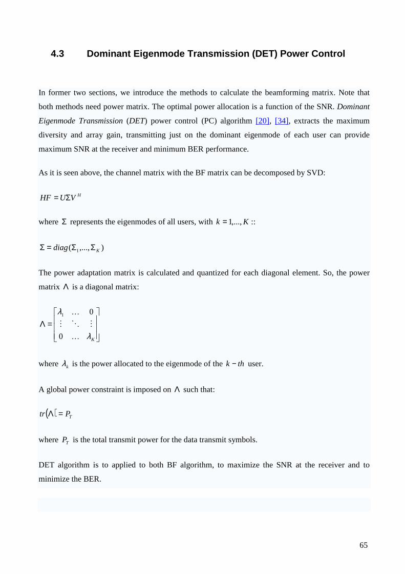
4.3 Dominant Eigenmode Transmission (DET) Power Control
In former two sections, we introduce the methods to calculate the beamforming matrix. Note that
both methods need power matrix. The optimal power allocation is a function of the SNR. Dominant
Eigenmode Transmission (DET) power control (PC) algorithm [20], [34], extracts the maximum
diversity and array gain, transmitting just on the dominant eigenmode of each user can provide
maximum SNR at the receiver and minimum BER performance.
As it is seen above, the channel matrix with the BF matrix can be decomposed by SVD:
HVUHF Σ=
where Σ represents the eigenmodes of all users, with Kk ,...,1= ::
),...,( 1 Kdiag ΣΣ=Σ
The power adaptation matrix is calculated and quantized for each diagonal element. So, the power
matrix Λ is a diagonal matrix:
=Λ
Kλ
λ
K
MOM
K
0
01
where kλ is the power allocated to the eigenmode of the thk − user.
A global power constraint is imposed on Λ such that:
( ) TPtr =Λ
where TP is the total transmit power for the data transmit symbols.
DET algorithm is to applied to both BF algorithm, to maximize the SNR at the receiver and to
minimize the BER.

66

67
Chapter 5
5. Simulation Results
This chapter will present MATLAB simulation results for the BF algorithms that were treated in the
previous chapter. In this section we evaluate the performance of a system employing the BF
technique. At the starting point, assuming perfect channel state information at the transmitter (CSIT),
SU-MIMO downlink BF is implemented to evaluate the link performance of the system, we quantify
the gap between a system with BF and a system without BF, just for one user. Moremore, two MU-
MIMO downlink BF algorithm ZF and SMMSE are investigated to evaluate and to compare the
performance of the system at the link-level by averaging the BERs and THs of all candidate users.
Finally, DET power control algorithm is to applied to both to maximize the SNR at the receiver and
to minimize the BER. As a case study, a link-level simulator complying UTRAN-LTE standard is
considered.
68
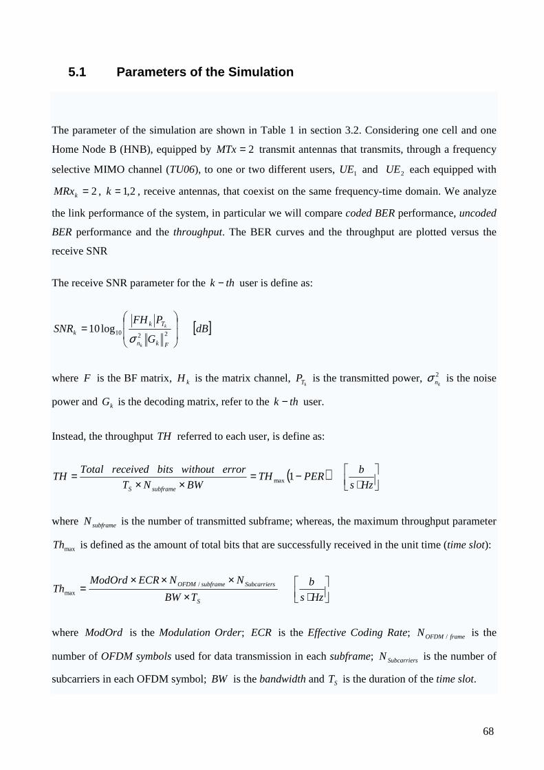
5.1 Parameters of the Simulation
The parameter of the simulation are shown in Table 1 in section 3.2. Considering one cell and one
Home Node B (HNB), equipped by 2=MTx transmit antennas that transmits, through a frequency
selective MIMO channel (TU06), to one or two different users, 1UE and 2UE each equipped with
2=kMRx , 2,1=k , receive antennas, that coexist on the same frequency-time domain. We analyze
the link performance of the system, in particular we will compare coded BER performance, uncoded
BER performance and the throughput. The BER curves and the throughput are plotted versus the
receive SNR
The receive SNR parameter for the thk − user is define as:
[ ]dBG
PFHSNR
Fkn
Tkk
k
k
=
2210log10σ
where F is the BF matrix, kH is the matrix channel, kTP is the transmitted power, 2
knσ is the noise
power and kG is the decoding matrix, refer to the thk − user.
Instead, the throughput TH referred to each user, is define as:
( )
⋅−=
××=
Hzs
bPERTH
BWNT
errorwithoutbitsreceivedTotalTH
subframeS
1max
where subframeN is the number of transmitted subframe; whereas, the maximum throughput parameter
maxTh is defined as the amount of total bits that are successfully received in the unit time (time slot):
⋅××××
=Hzs
b
TBW
NNECRModOrdTh
S
sSubcarriersubframeOFDM /max
where ModOrd is the Modulation Order; ECR is the Effective Coding Rate; frameOFDMN / is the
number of OFDM symbols used for data transmission in each subframe; sSubcarrierN is the number of
subcarriers in each OFDM symbol; BW is the bandwidth and ST is the duration of the time slot.
69
5.2 Beamforming for Single User
Here, we analyze the performance obtained with and without the beamforming technique for single
user; in particular we compare coded BER performance, uncoded BER performance and the
throughput either without BF or with BF. First simulations are conducted using a QPSK modulation
and an Effective Code Rates equal to 31 ( 31=ECR ). Then, the modulation used is a 16-QAM.
Every curve is plotted versus the SNR.
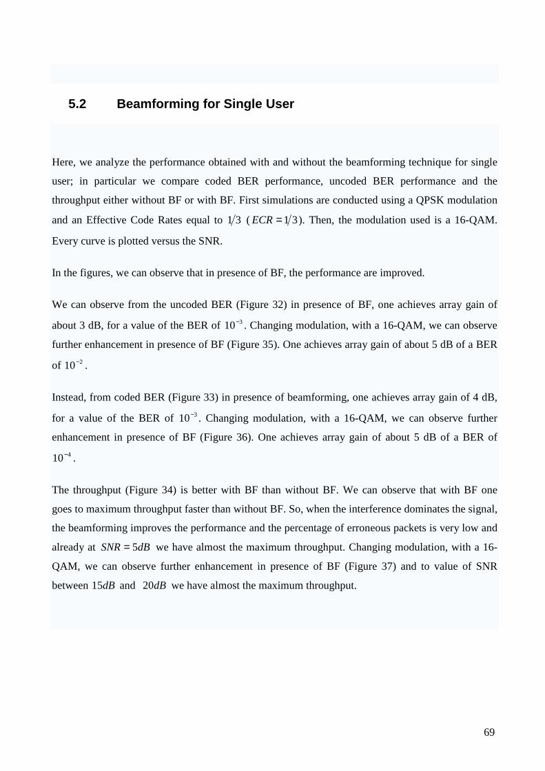
In the figures, we can observe that in presence of BF, the performance are improved.
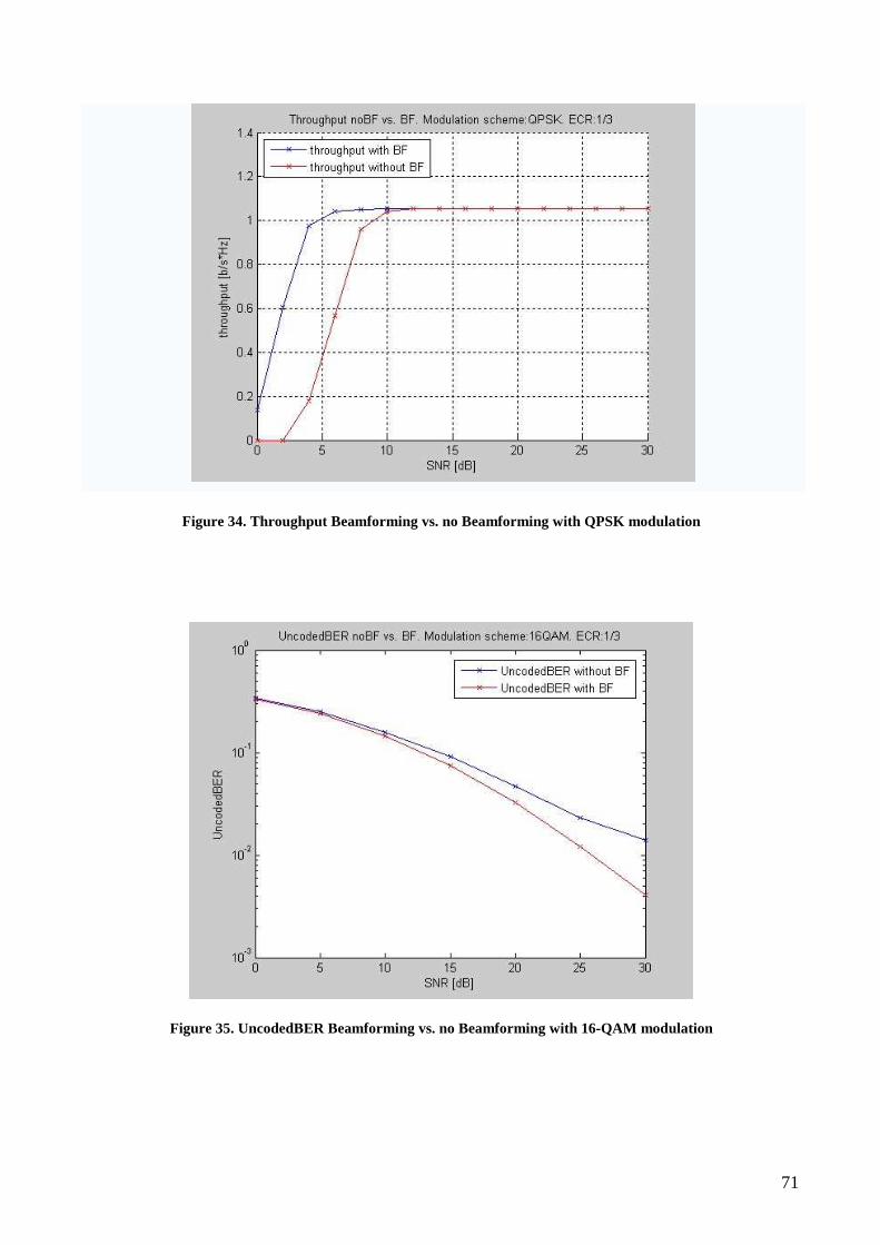
We can observe from the uncoded BER (Figure 32) in presence of BF, one achieves array gain of
about 3 dB, for a value of the BER of 310− . Changing modulation, with a 16-QAM, we can observe
further enhancement in presence of BF (Figure 35). One achieves array gain of about 5 dB of a BER
of 210− .
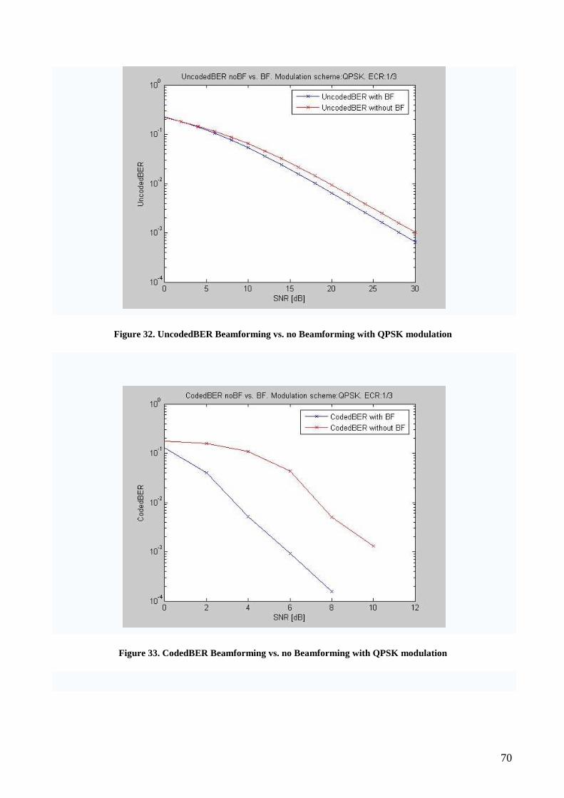
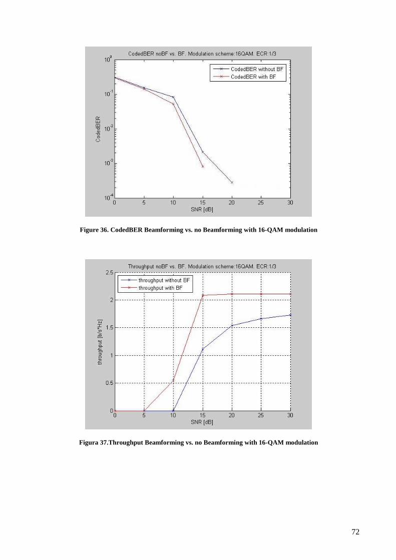
Instead, from coded BER (Figure 33) in presence of beamforming, one achieves array gain of 4 dB,
for a value of the BER of 310− . Changing modulation, with a 16-QAM, we can observe further
enhancement in presence of BF (Figure 36). One achieves array gain of about 5 dB of a BER of
410− .
The throughput (Figure 34) is better with BF than without BF. We can observe that with BF one
goes to maximum throughput faster than without BF. So, when the interference dominates the signal,
the beamforming improves the performance and the percentage of erroneous packets is very low and
already at dBSNR 5= we have almost the maximum throughput. Changing modulation, with a 16-
QAM, we can observe further enhancement in presence of BF (Figure 37) and to value of SNR
between dB15 and dB20 we have almost the maximum throughput.
70
Figure 32. UncodedBER Beamforming vs. no Beamforming with QPSK modulation
Figure 33. CodedBER Beamforming vs. no Beamforming with QPSK modulation
71
Figure 34. Throughput Beamforming vs. no Beamforming with QPSK modulation
Figure 35. UncodedBER Beamforming vs. no Beamforming with 16-QAM modulation
72
Figure 36. CodedBER Beamforming vs. no Beamforming with 16-QAM modulation
Figura 37.Throughput Beamforming vs. no Beamforming with 16-QAM modulation
73
5.3 Beamforming for Multi-User
In this section we analyze the performance obtained with the beamforming technique in Multi-User
case using the two methods, ZF and SMMSE, described in the section 4.1 and 4.2. In particular we
compare the coded BER performance, uncoded BER performance and the throughput between ZF-
BF and SMMSE-BF. The simulations are conducted using a QPSK modulation and an Effective
Code Rates equal to 32 ( 32=ECR ). Every curve is plotted versus the SNR.
In the figures, we can observe that with SMMSE method, the performance are improved.
We can observe from the uncoded BER (Figure 38) that SMMSE for a value of the BER of
410− provides a array gain of about 3 dB over ZF.
Instead, from coded BER (Figure 39) we can observe that SMMSE, for a value of the BER of 210− ,
provides a array gain of about 3 dB over ZF. We can also observe that SMMSE provides a diversity
gain of about 0.5 dB over ZF.
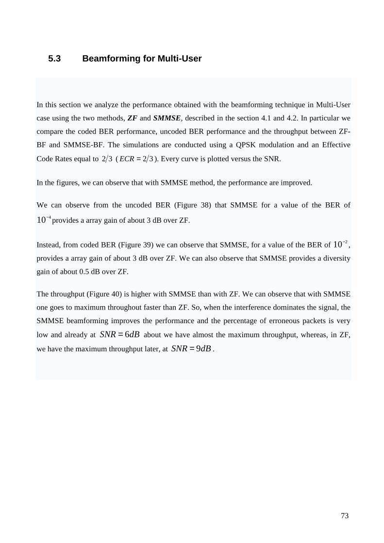
The throughput (Figure 40) is higher with SMMSE than with ZF. We can observe that with SMMSE
one goes to maximum throughout faster than ZF. So, when the interference dominates the signal, the
SMMSE beamforming improves the performance and the percentage of erroneous packets is very
low and already at dBSNR 6= about we have almost the maximum throughput, whereas, in ZF,
we have the maximum throughput later, at dBSNR 9= .

74
Figure 38. UncodedBER ZF vs SMMSE
Figure 39. CodedBER ZF vs SMMSE
75
Figure 40. Throughput ZF vs SMMSE
76
5.4 Beamforming for Multi-User with Power Control
In this section we analyze the performance obtained with the beamforming technique in Multi-User
case using the two methods, SMMSE, described in the section 4.1 and 4.2. In addition, we apply
Dominant Eigenmode Transmission (DET). In particular we compare the coded BER performance,
uncoded BER performance and the throughput between ZF-BF and SMMSE-BF. The simulations
are conducted using a QPSK modulation and an Effective Code Rates equal to 31 ( 31=ECR ).
Every curve is plotted versus the SNR.
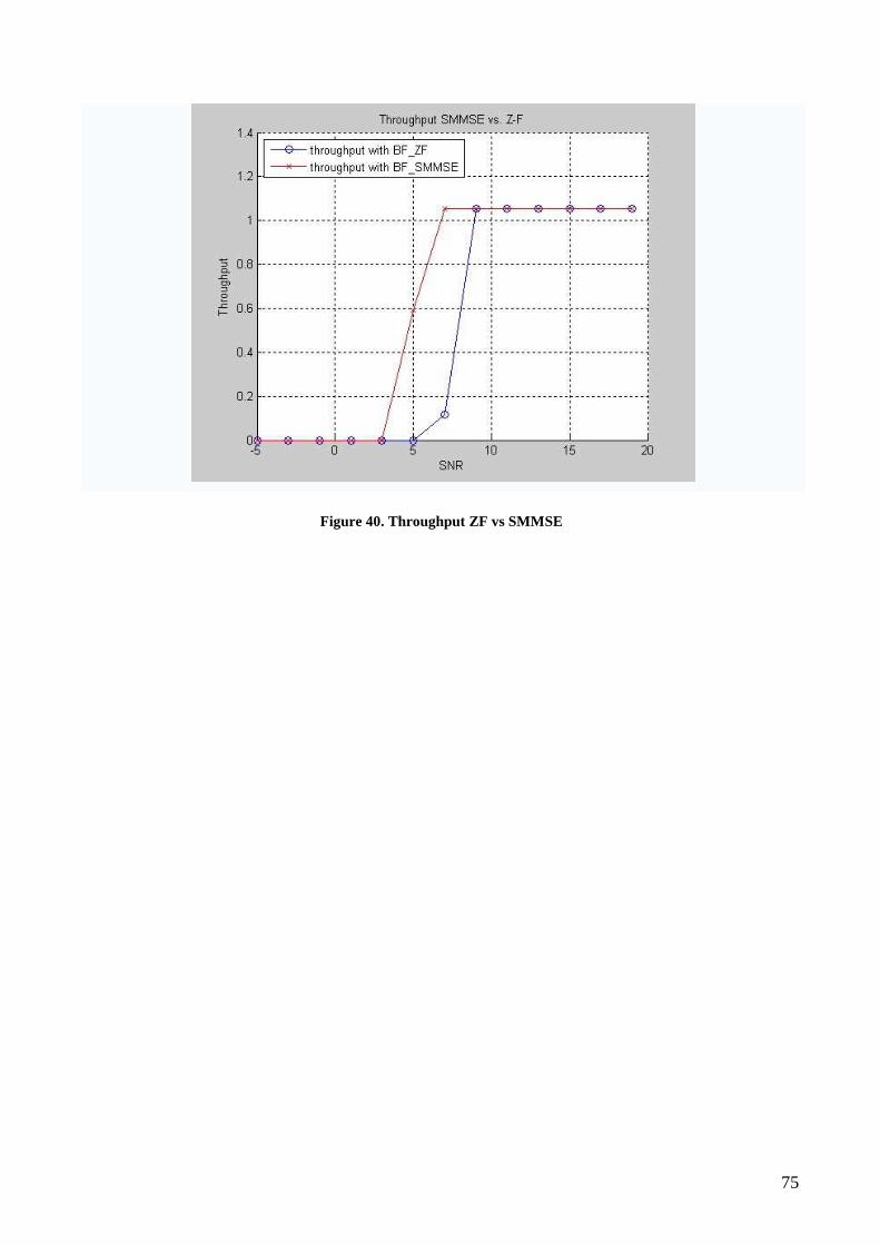
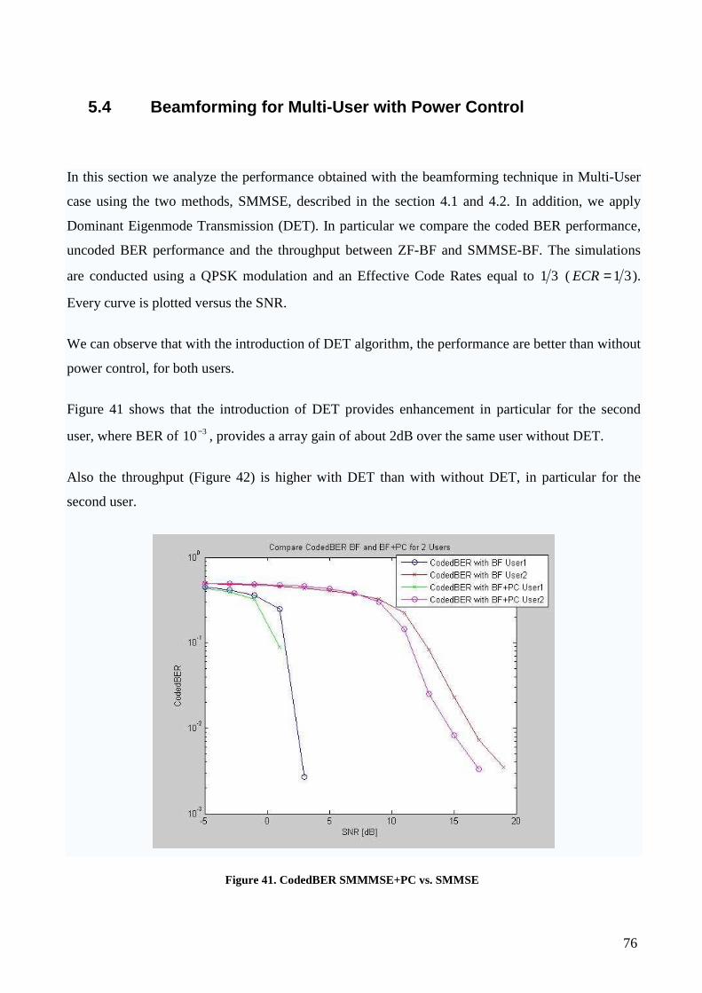
We can observe that with the introduction of DET algorithm, the performance are better than without
power control, for both users.
Figure 41 shows that the introduction of DET provides enhancement in particular for the second
user, where BER of 310− , provides a array gain of about 2dB over the same user without DET.
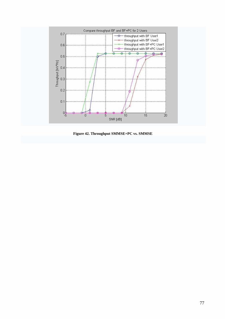
Also the throughput (Figure 42) is higher with DET than with without DET, in particular for the
second user.
Figure 41. CodedBER SMMMSE+PC vs. SMMSE
77
Figure 42. Throughput SMMSE+PC vs. SMMSE

78

79
Chapter 6
6. Conclusion and Future work
In this final chapter, the work undertaken in this thesis will be summarised with an emphasis on the
overall conclusions. In add, some suggestions for the future work will be also presented.
80
6.1 Conclusion
This thesis considered a beamforming and power control algorithm for MU downlink MIMO-
OFDM systems. Particulary, LTE system with FSU concept.
The major advantage of FSU is a better spectral scalability of the system than another spectrum
management. FSU is considered to occupy scarce spectral resources opportunistically in order to
increase the average spectral efficiency of the system and provide less interference to the order
system. So, to avoid interference to other systems, beamforming and power control algorithms are
investigated and implemented in MATLAB. As a starting point, assuming perfect channel state
information at the transmitter, single-user (SU) multiple input multiple output (MIMO) downlink
beamforming is implemented to evaluate the link performance of the system. As a case study, a
link-level simulator complying UTRAN Long Term Evolution (LTE) standard is considered.
Moreover, two multi-user (MU) MIMO downlink with OFDM/SDMA access scheme, beamforming
algorithms zero-forcing (ZF) and successive minimum mean square error (SMMSE) are
investigated to evaluate performance of the system at link-level by averaging the bit error rates
(BERs) and throughputs (THs) of all the candidate users. Numerical simulation results show
significant gains by 3dB to 5 dB, depending of the modulation using, and 3dB about, for the low
SNR, for the considered 22× system in terms of BER and TH, respectively, compared to the same
considered system without beamforming.
Simulation results showed, also, that SMMSE beamforming reduces the performance loss due to
zero MUI constraint and the cancellation of the interference between the antennas located at the
same terminal. Through our investigation for the considered system, it can be comprehended that
SMMSE outperforms ZF technique. SMMSE has relatively low computational complexity. Another
big advantage of SMMSE is that the users can be equipped with more antennas, so the total number
of receive antennas in the downlink can be greater than the number of transmit antennas.
Furthermore, this technique is especially useful at low SNRs, as the results have showed. Finally,
SMMSE provides higher array gain than ZF. Our results show significant gains by 3 dB and 3 dB,
in terms of BER and TH, respectively, comparing SMMSE to ZF beamforming algorithm.
The introduction of the DET algorithm improves further the performance of the system. Dominant
eigen transmission (DET) power algorithm is to applied to both to maximize the SNR at the receiver
and to minimize the BER.
BF and PC avoid co-channel interference and minimize the total transmitted power and this is
exactly the problem that is been considered here; i.e., how to choose the transmit BF vectors such
81
that the total transmitted power is minimized while the system provides an acceptable Quality of
Service (QoS) serving as many users as possible.
This treats just a single MU-MIMO system. In fact, her we limit our study to the single cell case; i.e.
we do not consider the interference from other neighboring cells. An interesting approach would be
to use SMMSE with interference inter-cell MU-MIMO system, when the cells are in cooperative
mode and/or no. An another interesting approach would be to use a non-linear beamforming
techniques and compare it with the SMMSE technique.

82
83
Bibliography
[1] J. Mitola et al., “Cognitive Radio: Making Software Radios more personal”, IEEE Pers.
Commun., Vol. 6, no. 4, August 1999.
[2] P. J. Kolodzy, “Cognitive Radio Fundamentals”, SDR Forum, Singapore, April 2005.
[3] R. W. Chang, “Synthesis of band-limited orthogonal signals for multichannel data
transmission”, Bell Systems Technical Journal, 45:1775-1796, 1966.
[4] DuŽan Matiaæ, “OFDM as a possible modulation technique for a multimedia applications in
the range of mm waves”, 1998.
[5] H. Codina, S. Rene, “Performance study of SC-FDMA and OFDMA for uplink in evolved
UTRA”, Project group MOBCOM-1114, Institute of Electronic System Department of
Communication Technology, Aalborg University, September 2006.
[6] V. Venkataraman, J. J. Shynk, “Adaptive Interference Suppression in Multiuser OFDM”,
IEEE Vehicular Technology Conference, (Santa Barbara, CA), vol.1, pp. 655-659, 2005.
[7] H. Rohling, R. Grunheid, “Performance comparison of different multiple access schemes for
the downlink of an OFDM communication system”, Proc. IEEE Vehicular Technology
Conference, (Phoenix, AZ), pp1365-1369, May 1997.
[8] D. V. P. Figueiredo, M. I. Rahman, N. Marchetti, F. H. P. Fitzek, M. D. Katz, Y. Cho, R.
Prasad, “Transmit Diversity Vs Beamforming for Multi-User OFDM System”, Wireless
Personal Mobile Communications, Abam Terme, Italy, September 2004.
[9] P. Vandenameele, L. Van Der Perre, M. Engels, B. Gyselinckx, H. De Man, "A Combined
OFDM/SDMA Approach”, IEEE J. Select. Areas Commun., vol.18, pp. 2312-2321,
Nov.2000.
84
[10] C. I. Yeh, D. S. Kwon, “SDMA, Multiuser Diversity, and BF Using Antenna Array in
OFDMA System”, IEEE Vehicular Technology Conference, 2007.
[11] T. A. Thomas, B. Mondal, K. L. Baum, F. W. Vook, “User Selection for SDMA
Beamforming with Imperfect CSI in MIMO-OFDM System”, IEEE International
Conference, June 2007.
[12] B. D. Van Veen, K. M. Buckley, “Beamforming: A Versatile Approach to Spatial
Filtering”, IEEE ASSP Magazine, April 1988.
[13] J. Litva, T. Kwok-Yeung Lo “Digital Beamforming in Wireless Communications”, Arthec
House, Boston (Londra), 1996.
[14] A. Alexious et al., “Assessment of Advanced Beamforming and MIMO Technologies”,
IST-2003-507581 WINNER, D2.7 ver. 1.1, February 2005.
[15] A. Gershman, “MIMO Communications and Space-Time Coding”, Institute F.
Nachrichtentechnik, FG Nachrichtentechnische Systeme (NTS), TU Darmstadt, April 2005.
[16] A. J. Paulraj, Gore, Choi, Nettles, “An Overview of MIMO Communications. A key to
Gigabit Wireless”, IEEE Trans Comm, 2003.
[17] H. Ganapatly, “MIMO System: Basic principles, Algorithms and Networking
Applications”, www.cse.buffalo.edu/~qiao/cse620/fall04/mimo.ppt.
[18] M. Vu, A. Paulraj, “MIMO Wireless Linear Precoding”, IEEE Signal Processing
Magazine, February 2006.
[19] Q. H. Spencer, A. Lee Swindlehurst, M. Haardt, “Zero-Forcing Methods for Downlink
Spatial Multiplexing in Multiuser MIMO Channels”, IEEE Transactions on Signal
Processing, Vol. 52, No. 2, February 2004.
85
[20] V. Stankovic, M. Haardt, “Multi-User MIMO Downlink Precoding for User with Multiple
Antennas”, Proceedings of the 12th Meeting of the Wireless World Research Forum (wwrf
’04), Toronto, Ontario, Canada, November 2004.
[21] B. Bandemer, M. Haardt, S. Visuri, “Linear MMSE Multi-User MIMO Dowlink
Precoding for Users with Multiple Antennas”, The 17th Annual IEEE International
Symposium on Personal, Indoor and Mobile Radio Communications, 2006.
[22] I.F Akyildiz, Won-Yeol Lee, M.C. Vuran, S. Mohanty, “NeXt generation/dynamic
access/cognitive radio wireless networks: A survey”, Computer Networks, Atlanta (GA),
May 2006.
[23] 3GPP Technical Specification Group Radio Access Networks, “Deployment aspects
(Release 4)” , 3GPP TR 25.943 V4.2.0, 2006.
[24] Qualcomm Incorporation, “LTE- A Well-Designed Mobile OFDMA IP Solution”,
January 2008.
[25] Nortel Networks, “Long-Term Evolution (LTE): The vision beyond 3G”, 2007.
[26] A. Paulraj, R.Nabar, D. Gore, “Introduction to Space-Time Wireless Communications”,
Cambridge University Press, 2003.
[27] International Telecommunication Union, “Draft Guidelines for Evaluation of Radio
Transmission Technologies for IMT-Advanced”, Document 8F/TEMP/495-E, Tech. Rep.,
January 2007.
[28] S. Kumar, G. Costa, S. Kant, F.B. Frederiksen, N. Marchetti, P. Mogensen, “Spectrum
Sharing for Next Generation Wireless Communication Network”, Radio Access Technology
Section (RATE), Aalborg University, Denmark, 2007.
[29] WINNER D6.1, “WINNER Spectrum Aspects: Methods for efficient sharing, flexible
spectrum use and coexistence”, IEEE 802.16 Broadband Wireless Access Working Group,
Tech. Rep., IST-2003-50758.
86
[30] 3GPP TS 36.300 V8.2.0 (2007-09); 3rd Generation Partnership Project; Technical
Specification Group radio Access Network; Overall Description; Stage 2 (Release 8).
[31] 3GPP TS 36.211 V8.0.0 (2007-09); 3rd Generation Partnership Project; Technical
Specification Group radio Access Network; Physical Channel and Modulation (Release 8).
[32] 3GPP TS 36.214 V8.0.0 (2007-09); 3rd Generation Partnership Project; Technical
Specification Group radio Access Network; Physical Layer; Measurements (Release 8).
[33] 3GPP TS 36.401 V1.0.0 (2007-09); 3rd Generation Partnership Project; Technical
Specification Group radio Access Network; Physical Layer; Measurements (Release 8).
[34] T. See Ho, K. Sakaguchi, K. Araki, “Performance Analysis of MIMO Eigenmodes
Transmission System Under Realistic Channel and System Conditions”, IEEE Transactions
on Signal Processing, Vol. E87-B, No. 8, pp. 2222-2232, August 2004.

87

88
Appendix A
Channel Profiles
Radio wave propagation in the mobile environment can be described by multiple paths which arise
due to reflection and scattering in the mobile environment [23]. Approximating these paths as a
finite number of N distinct paths, the impulse response for the radio channel may be written as:
∑=
⋅=N
iiiah
1
)()( τδτ
which is the well known tapped-delay line model. Due to scattering of each wave in the vicinity of a
moving mobile, each path ia will be the superposition of a large number of scattered waves with
approximately the same delay. This superposition gives rise to time-varying fading of the path
amplitudes ia , a fading which is well described by Rayleigh distributed amplitudes varying
according to a classical Doppler spectrum:
5,02
1
1)(
−
∝
Df
ffS
where λv
fD = is the maximum Doppler shift, a function of the mobile speed v and the wavelength
λ . In some cases a strong direct wave or specular reflection exists which gives rise to a non-fading
path, then the Doppler spectrum is:
)()( SffS δ=
where Sf is the Doppler frequency of the direct path, given by its direction relative to the mobile
direction of movement.
The channel models presented here will be described by a number of paths, having average powers
2
ia and relative delays iτ , along with their Doppler spectrum which is either classical or a direct
path. The models are named TUx (Typical Urban), RAx (Rural Area), HTx (Hilly Terrain), where
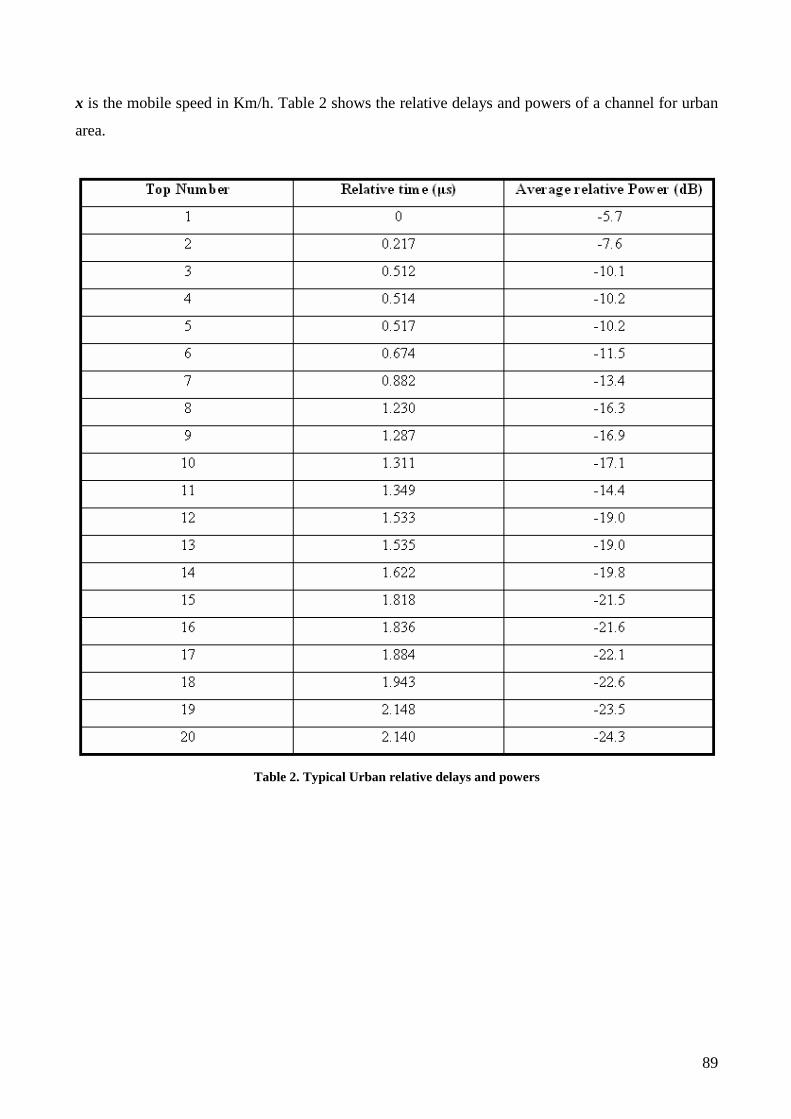
89
x is the mobile speed in Km/h. Table 2 shows the relative delays and powers of a channel for urban
area.
Table 2. Typical Urban relative delays and powers
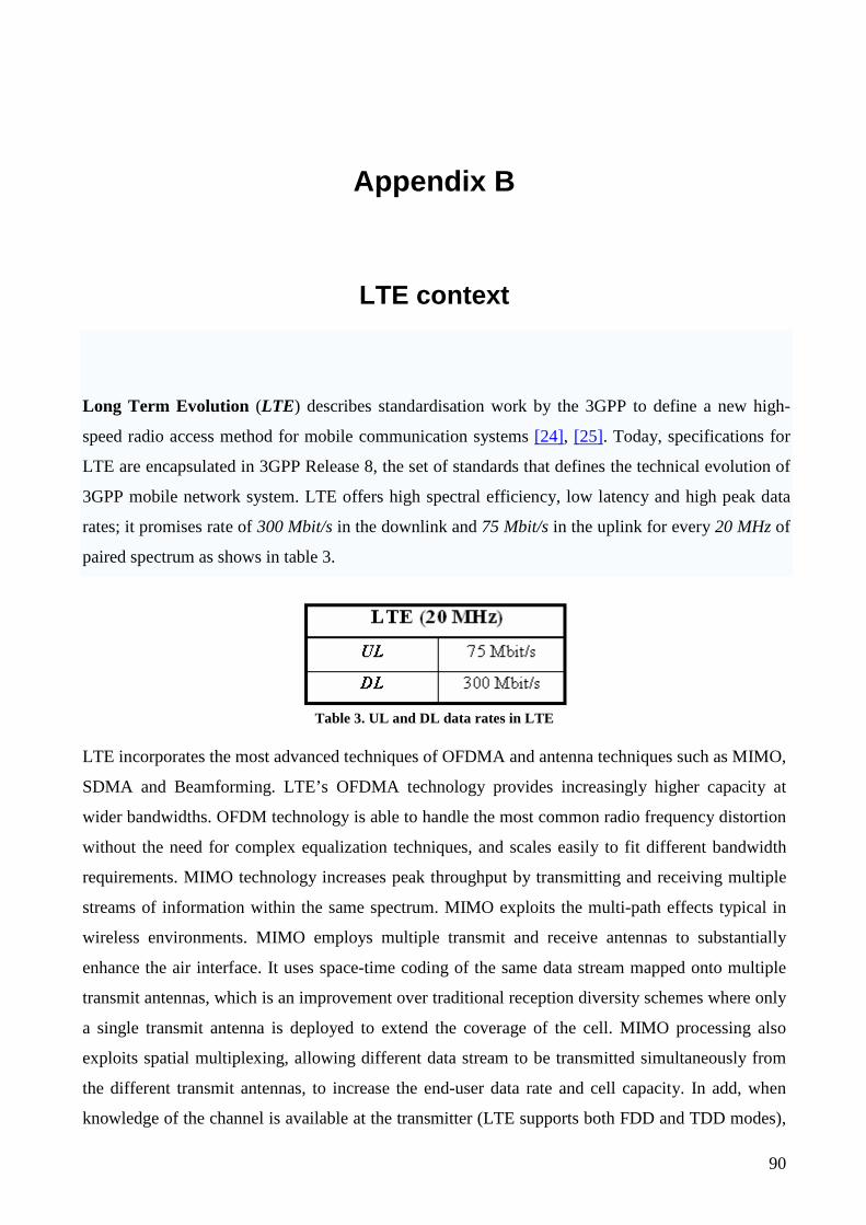
90
Appendix B
LTE context
Long Term Evolution (LTE) describes standardisation work by the 3GPP to define a new high-
speed radio access method for mobile communication systems [24], [25]. Today, specifications for
LTE are encapsulated in 3GPP Release 8, the set of standards that defines the technical evolution of
3GPP mobile network system. LTE offers high spectral efficiency, low latency and high peak data
rates; it promises rate of 300 Mbit/s in the downlink and 75 Mbit/s in the uplink for every 20 MHz of
paired spectrum as shows in table 3.
Table 3. UL and DL data rates in LTE
LTE incorporates the most advanced techniques of OFDMA and antenna techniques such as MIMO,
SDMA and Beamforming. LTE’s OFDMA technology provides increasingly higher capacity at
wider bandwidths. OFDM technology is able to handle the most common radio frequency distortion
without the need for complex equalization techniques, and scales easily to fit different bandwidth
requirements. MIMO technology increases peak throughput by transmitting and receiving multiple
streams of information within the same spectrum. MIMO exploits the multi-path effects typical in
wireless environments. MIMO employs multiple transmit and receive antennas to substantially
enhance the air interface. It uses space-time coding of the same data stream mapped onto multiple
transmit antennas, which is an improvement over traditional reception diversity schemes where only
a single transmit antenna is deployed to extend the coverage of the cell. MIMO processing also
exploits spatial multiplexing, allowing different data stream to be transmitted simultaneously from
the different transmit antennas, to increase the end-user data rate and cell capacity. In add, when
knowledge of the channel is available at the transmitter (LTE supports both FDD and TDD modes),
91
MIMO can also implement Beamforming to further increase available data rates and spectrum
efficiency.
92
Appendix C
TDD System
Beamforming is a processing technique that use CSIT by operating on the signal before transmission
[18], [26]. In fact, the transmitter can only know CSI indirectly; whereas, the receiver can estimate
the channel directly from the channel-modified received signal. Pilots are usually inserted in the
transmitted signal to facilitate channel estimation by the receiver. There are two principles for
obtained CSIT: reciprocity and feedback. Reciprocity involves using the reverse channel information
(open-loop), while feedback requires sending the forward channel information back to the
transmitter (closed loop). Both reciprocity and feedback methods are used in practical wireless
systems, including Time-Division-Duplex (TDD) and Frequency-Division-Duplex (FDD). TDD
systems may use reciprocity techniques. While the forward and reverse links in a TDD system often
have identical frequency bands and antennas, there is time lag is the scheduling delay between the
reception of the signal from a user and the next transmission to that user. Such time lags must be
negligible compared to the channel coherence time for reciprocity techniques to be applicable. FDD
systems, on the other hand, usually have identical temporal and spatial dimensions on the forward
and reverse links, but the link frequency offset is often much larger the channel coherence
bandwidth, making reciprocity techniques infeasible. FDD systems therefore commonly use
feedback techniques.
The reciprocity principle in duplex transmission, the transmitter (HNB) first estimates the reverse
link channel, and uses this estimate for the forward link channel. Let us discuss a SISO case. Let
),,( ffff ifth be the forward SISO channel from HNB transmitter antenna to the user and
),,( rrrr ifth be the reserve SISO channel, as show in figure 44. where, ft , ff and fi refer to the
time, frequency and antenna index used on the forward link; whereas rt , rf and ri are similarly
defined for the reverse link. The antenna index specifies the antenna used at the HNB and the user.
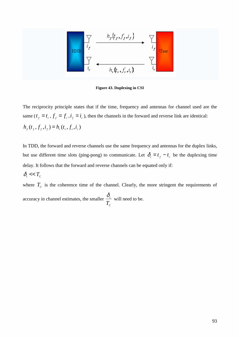
93
Figure 43. Duplexing in CSI
The reciprocity principle states that if the time, frequency and antennas for channel used are the
same ( rf tt = , rf ff = , rf ii = ), then the channels in the forward and reverse link are identical:
),,(),,( rrrrffff ifthifth =
In TDD, the forward and reverse channels use the same frequency and antennas for the duplex links,
but use different time slots (ping-pong) to communicate. Let rft tt −=δ be the duplexing time
delay. It follows that the forward and reverse channels can be equated only if:
Ct T<<δ
where CT is the coherence time of the channel. Clearly, the more stringent the requirements of
accuracy in channel estimates, the smaller C
t
T
δ will need to be.

94
Acknowledgement
…So, I’m at the last pages of my thesis….
…I think these are more difficult than another pages, but I will try to write them…
I would like to thank everybody that I have met in these years! I hope to not forget anyone…
This is a logic order not by importance, everybody are very important in my life!
I would like to say thank to…
My supervisors Nicola Marchetti and Shashi Kant for their support and encouragement during the
development of this project. Even more important than the wise advice they always gave me, I
deeply appreciate the friendly atmosphere in which we worked together. I want to acknowledge the
effort and time they spent trying to lead me to a higher level.
Nicola, grazie, because, nothing is impossible…
Shashi शु�बयाशु�बयाशु�बयाशु�बया, because, the great man are also small…
Gila, for the contribution to the work, because you are a genius, because, without you, I was not
able to continue the work…
My Prof. Roberto Cusani for the possibility of this fantastic experience! And for all advices given.
Grazie Prof…
Luna people, Francesco, Jordi, Jop, Pepe, Sergio, Sam, Milos, David, Flora, Berenicè, Richard,
Borja, Michal and others, for the beautiful atmosphere in the Luna Kollegium, for the crazy party,
for the pussy-man, for the fisherman, for the great moments that we shared together…
All the friends I have met here from all around the world, specially the ones I will most miss and the
ones with who I will keep in contact. Thanks for showing me that there is life in Aalborg despite of
its wonderful weather. I will always remember the great moments we shared together…
Now I begin to write in Italian…
…oh sorry!!! I don’t speak Italian…
…I will continue in Roman languages…
Unlook!!!
95
Ai miei genitori, le persone senza le quali non sarei mai diventato quello che sono, sempre attenti,
affettuosi, disponibili!!Hanno sempre creduto in me, non mi hanno mai fatto mancare niente!!! Mi
hanno dato la migliore educazione che si potesse mai avere!!!
Rinco, è sempre bastato un cenno tra di noi, non siamo di tante parole (a parte la Roma..), ma tanto
non servono…
Gigliola, bè che dire, oddio rompe le scatole, però nessuno avrebbe mai fatto quello che ha fatto lei
per me, anzi per noi. E poi la pizza, gli spaghetti al cartoccio, la pasta al forno, gli gnocchi, mejo
smette che me sta a pijà fame…E poi è inutile aggiungere altro se no questa se mette a piagne pe ‘na
decina d’anni…
Ciccio, mio fratello, anzi FRATELLONE, ogni volta che stai giù, che sei stanco, che ti sei stufato di
tutto e di tutti, basta guardarlo, guardi la sua faccia simpatica e tutto passa. Qui in Danimarca me sei
mancato da morì!!! Non esiste un fratello migliore!!! Grazie per tutte le volte che abbiamo preso in
giro Gil e Rinco insieme. Lo sai benissimo che il prossimo a scrive sti commenti sulla tesi sei tu!! E
poi ho bisogno di un dottore in biologia! Daje Ciccio!!!!
Zio Renato, ecco già c’ho le lacrime agli occhi…, quanto me manchi zi…,te dico solo grazie se no
non continuo più a scrive…
Zio Enrico, magari non l’ho conosciuto troppo a fondo, però mi ha lasciato il ricordo di una grande
persona…
I miei nonni Giovannella e Francesco, Maria e nonno, c’è chi ho conosciuto di più, chi di meno, chi
per niente, ma in fondo senza di voi non starei qui…
I miei cugini vicini e lontani perché ci sono sempre quando ne hai bisogno, in particolare un grazie
speciale a:
Francesco, che ha trattato con cura i miei capelli e ora si vedono i risultati (non ce l’ho più…), una
persona fantastica, schietta e sincera, da lui si può solo apprendere, ovviamente solo per quel che
riguarda le scommesse sportive, tutto lo sport in generale, ma in particolare il suo linguaggio…
Alex, cugì, ormai io e te semo come du carabinieri, inseparabili…, anche da lontano, grazie…
Alessandra e Valeria, per le loro lacrime anche quando non c’è ne bisogno e per il loro affetto e per
ogni volta che ricordiamo i momenti dell’infanzia passati insieme…
Pamela, Vittorio, Fabrizio, perché credono che sia un genio…
96
I miei zii Pietro e Anna Maria, Vincenzo e Anna, Peppe e Rita, Domenico e Maria, Teresa, Ernesto
e Rita, Dino e Ferrina, Giuseppe Anna Rita, Lucio e Silvia, mi hanno trattato tutti come un loro
figlio, è un onore essere vostro nipote…
Roberto e Alessandra, per le serate a mangiare la pizza di mamma, per le risate e perché per me
sono semplicemente di famiglia…
Le mie sorelline Marta e Marzia, perché hanno occupato la mia camera per tutto il periodo che sono
stato in Danimarca…
Tania, perché è nata il mio stesso giorno, perché in tutte le “foto” più importanti dei miei ultimi 10
anni… te ci sei, perché nessuno mi conosce meglio di te…
Francesca, perché ho semplicemente ritrovato una sorella, che mi consiglia, che mi ascolta, che mi
rimprovera e che vuole farmi assolutamente fidanzare, ci riuscirà? Dubito…
I Buddhi, Gaetano, Claudia e Domenico, perché anche se non ci frequentiamo più così tanto spesso,
le giornate, le emozioni, le avventure passate insieme, ogni singolo ricordo è indelebile nel mio
cuore…
Sabrina, perché in questi anni, per alcuni mesi, studiare è stato più duro, la mente era sempre
lontana dai libri; perché anche se non fa più parte della mia vita, rimane una delle persone più
importanti…
Bruno, perché è il mio secondo padre e penso che non c’è bisogno di aggiungere altro…
Lisa e Natalia, tutti gli amici di Casali, Emiliano, Armando, Mazza, Russo, Daniela perché le
amicizie che durano da quindici anni non si possono dimenticare…
Serena, perché è stata in Danimarca con me, perché mi ha ospitato sul suo pavimento e perché c’ho
ragione sempre io e lei mai…
Bestia e Giuglia, perché sono la coppia più divertente del mondo, perché studiare con loro è stato
puro divertimento…
97
Claudia, Jenna, Anna, Palma, Fabbrica e Sità, Fabio e Conte, Claudio e Francesca, Carmine e tutti
gli altri amici dell’uni per tutti i pomeriggi passati all’uni a “studiare”, al chiostro, allo spaccio,…
Emy, Mary, Viola, Ilaria, per le lingue di gatto, per le lunghe pause di studio, perché sono delle
persone eccezionali, perché l’ho conosciute in modo buffo…
Loreto, per le video-chiamate all’una di notte, quando invece di mandarmi a quel paese fermava il
suo lavoro e mi ascoltava; per i consigli su matlab, per il grande aiuto su questa tesi, per i fagioli
alle 4 del mattino, le salsicce alle 6, per la barba non tagliata, perché io dalla Danimarca guardavo la
Roma e lui che stava a Roma no, perché è un grande amico…
Simona, per i messaggi di saluto su msn, perché verrà con me al concerto di Vasco, perché mi ha
fatto passare un capodanno “particolare”, perché vorrebbe ricambiare il favore, ma io non me
ubriaco mai, perché ho scoperto una persona speciale…
Le mie compagne di stanza di capodanno, Silvia, Ary mora, Ary bionda, Sara, perché mi hanno
fatto passare un gran capodanno, per le chiacchierate su msn, perché anche se stavo lontano, loro
erano vicine…
Tutti gli amici italiani conosciuti qui in Danimarca, Giampaolo (perché è più famoso della Coca
Cola), Jo-wow (perché è italiano no portoghese), Francesco cugino (per le simulazioni), Francesco
brother (perché è come un fratello), Filippo (perché mi ha insegnato il toscano), Mary (perché è
della Roma), Luca & Ane (per la cena danese), Mauro (perché è un pazzo), Valerio e Nicoletta
(perché sono unici), Avvocato (per il suo italiano), Chiara (perché non ha condiviso la stanza con
noi), Valentina (per la nutella), Stella (per le ricariche telefoniche e perché è troppo simpatica),
Francesco Ciccio (perché se no non mi manda alla student house), Anna (per il suo sorriso), Sara
(per le foto da ubriacona), Manu (per la sua disponibilità), Antonio (per la sua pizza), Davide (un
mito)…
Gli amici del laboratorio di Roma, Mauro, Christian, Nicola, MarioTilli, Massimo, Valeria perché le
giornate in laboratorio con loro erano uno spasso.
Valentina e Monica, per le serate passate insieme e perché mi sono sempre vicini…
Simone per la sua straordinaria simpatia…
98
Tutti gli amici del calcetto, perché fare tutti i tornei che ho fatto insieme a loro è stato un piacere ed
un onore!!! Perché hanno contribuito a farmi distrarre ed a tenermi in forma…
Ristorante i Leoni, Carlo, Elenia, Emanuele, Ringo, Franco, perché mi hanno dato la possibilità di
mantenermi gli studi e perché mi hanno fatto sentire una famiglia…
Tutti i miei alunni e alunne, perché mi fanno sentire importante, perché per loro sono e sarò per
sempre il loro Prof, perché mi hanno fatto vivere una delle più belle esperienze della mia vita,
perchè è stato un onore essere il loro insegnante, per tutto quello che mi hanno insegnato, perché
vogliono venirmi a vedere alla mia discussione (ma solo per saltare un giorno di scuola), perché non
li dimenticherò mai…
Tutte le persone che ho conosciuto nell’ambito scolastico, e che si sono sempre fatti sentire, che non
hanno interrotto i contatti, che già “ciao come vanno le cose in Danimarca?”, ti fanno sentire vicino
a loro, in particolare un grazie a Fabiola e a tutti quelli a cui ho fatto l’esame di maturità…
Tutti i miei colleghi Prof, perché mi hanno aiutato nella mia prima esperienza, per i consigli, perché
mi hanno voluto bene…
…Penso di aver ringraziato tutti, non manca nessuno…
… bè mancano 4 persone…
…per loro una vita intera di ringraziamenti non basta…
…per loro, però, basta una semplice riga …
… sono gli amici che tutti vorrebbero, perché …
…sono semplicemente una parte di me…
Fettina, perché è un FRATELLO…
Miky, perché è un AMICO…
Piastra, perché è un COMPAGNO…
Paolo, perché è un COMPLICE…
Grazie di cuore a tutti quanti, perchè tutti avete contribuito a questo mia tesi e perchè fate parte della
mia vita, e perché…
…senza di voi,…io non esisto…
Recommended