1
Beam-Beam Effects in
Particle Colliders
Mauro Pivi
SLAC
US Particle Accelerator School
January 17-21, 2011 in Hampton, Virginia
2
Particle physicist usually assume =c=1, in this context (next
5 pages only).
To compute the collision energy between particles, let’s
define a new entity: the particle energy E and the classical 3-
momentum p form a (Jargon point!) “4-momentum tensor”:
ˆ ( , )p E p
Center of mass energy in a collision
3
The scalar product between two particles momenta is defined
as:
And it is an “invariant” (reference frame independent).
Thus note that, since
where (=c=1!), then the product of the four-vector by itself is:
22 2ˆ ˆp p E m p
1 2 1 2
ˆ ˆp p E E1 2p p
2 22 2 4 2E c m c m p p
Center of mass energy in a collision
4
In a particle collision, the quantity:
is a Lorentz-invariant. The center-of-mass energy available for
physics experiments is:
cmE s
2
21)ˆˆ( pps
Center of mass energy in a collision
5
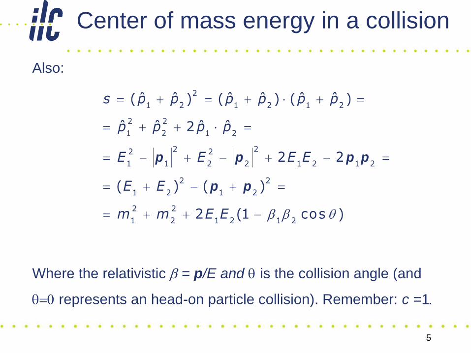
Also:
Where the relativistic b = p/E and q is the collision angle (and
q0 represents an head-on particle collision). Remember: c =1.
2
1 2 1 2 1 2
2 2
1 2 1 2
2 22 2
1 1 2 2 1 2 1 2
2 2
1 2 1 2
2 2
1 2 1 2 1 2
ˆ ˆ ˆ ˆ ˆ ˆ( ) ( ) ( )
ˆ ˆ ˆ ˆ2
2 2
( ) ( )
2 (1 cos )
s p p p p p p
p p p p
E E E E
E E
m m E E b b q
p p p p
p p
Center of mass energy in a collision
6
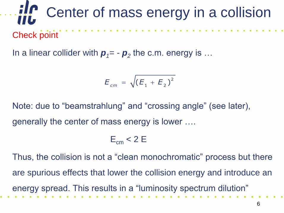
Check point
In a linear collider with p1= - p2 the c.m. energy is …
Note: due to “beamstrahlung” and “crossing angle” (see later),
generally the center of mass energy is lower ….
Ecm < 2 E
Thus, the collision is not a “clean monochromatic” process but there
are spurious effects that lower the collision energy and introduce an
energy spread. This results in a “luminosity spectrum dilution”
2
1 2( )
cmE E E
Center of mass energy in a collision
7
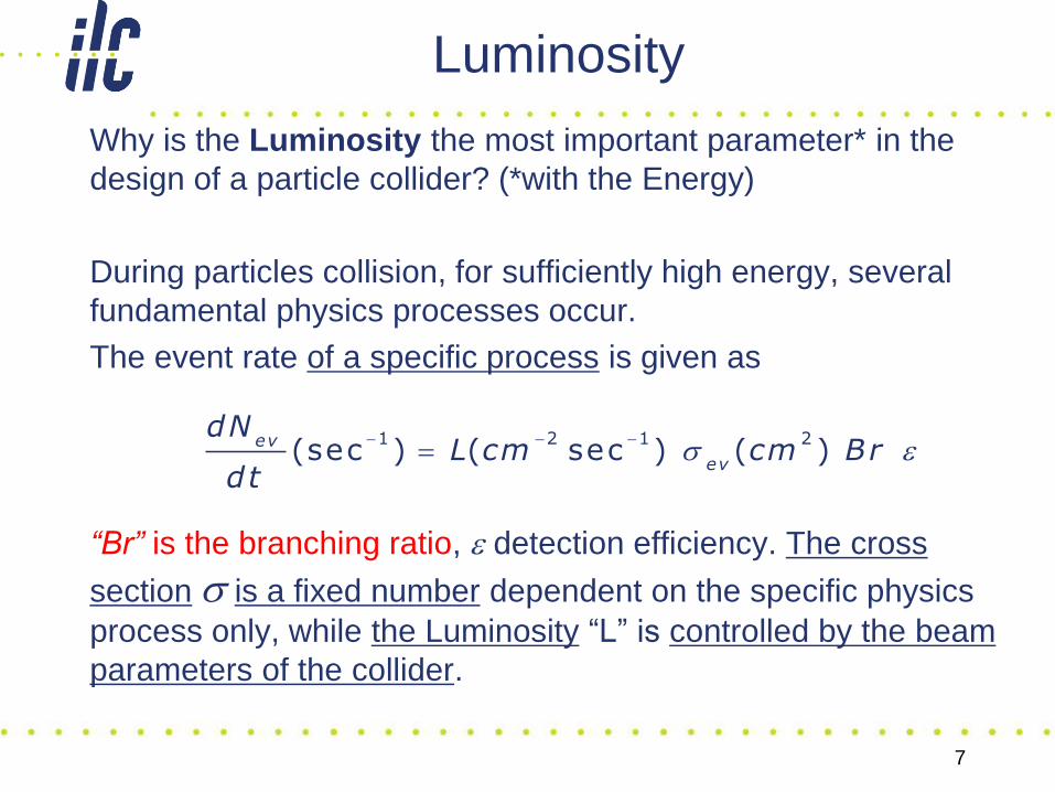
Why is the Luminosity the most important parameter* in the
design of a particle collider? (*with the Energy)
During particles collision, for sufficiently high energy, several
fundamental physics processes occur.
The event rate of a specific process is given as
“Br” is the branching ratio, e detection efficiency. The cross
section s is a fixed number dependent on the specific physics
process only, while the Luminosity “L” is controlled by the beam
parameters of the collider.
Luminosity
1 2 1 2(sec ) ( sec ) ( ) ev
ev
dNL cm cm Br
dts e
8
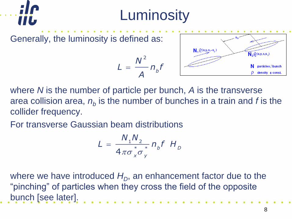
Generally, the luminosity is defined as:
where N is the number of particle per bunch, A is the transverse
area collision area, nb is the number of bunches in a train and f is the
collider frequency.
For transverse Gaussian beam distributions
where we have introduced HD, an enhancement factor due to the
“pinching” of particles when they cross the field of the opposite
bunch [see later].
Luminosity
2
b
NL n f
A
s s 1 2
* *
4b D
x y
N NL n f H
9
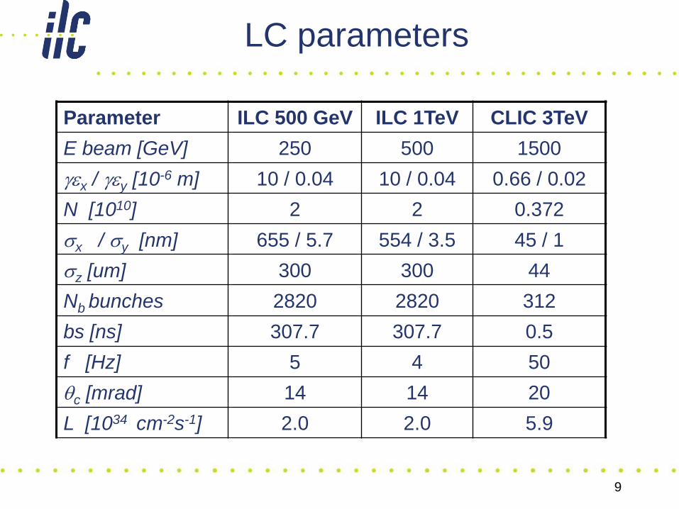
LC parameters
Parameter ILC 500 GeV ILC 1TeV CLIC 3TeV
E beam [GeV] 250 500 1500
gex / gey [10-6 m] 10 / 0.04 10 / 0.04 0.66 / 0.02
N [1010] 2 2 0.372
sx / sy [nm] 655 / 5.7 554 / 3.5 45 / 1
sz [um] 300 300 44
Nb bunches 2820 2820 312
bs [ns] 307.7 307.7 0.5
f [Hz] 5 4 50
qc [mrad] 14 14 20
L [1034 cm-2s-1] 2.0 2.0 5.9
10
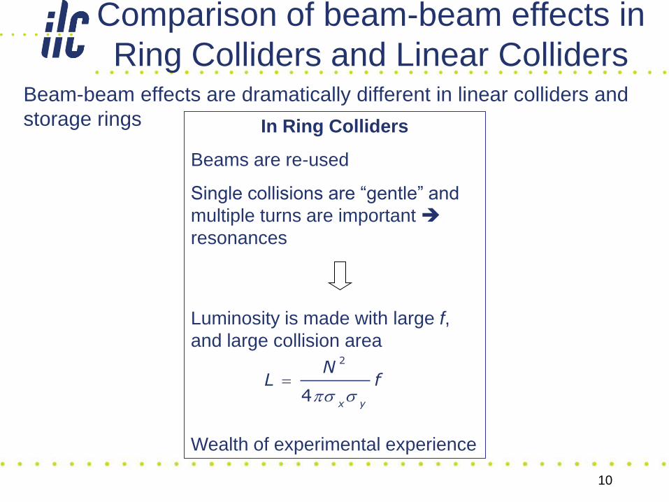
Comparison of beam-beam effects in
Ring Colliders and Linear CollidersBeam-beam effects are dramatically different in linear colliders and
storage rings In Ring Colliders
Beams are re-used
Single collisions are “gentle” and
multiple turns are important
resonances
Luminosity is made with large f,
and large collision area
Wealth of experimental experience
2
4x y
NL f
s s
11
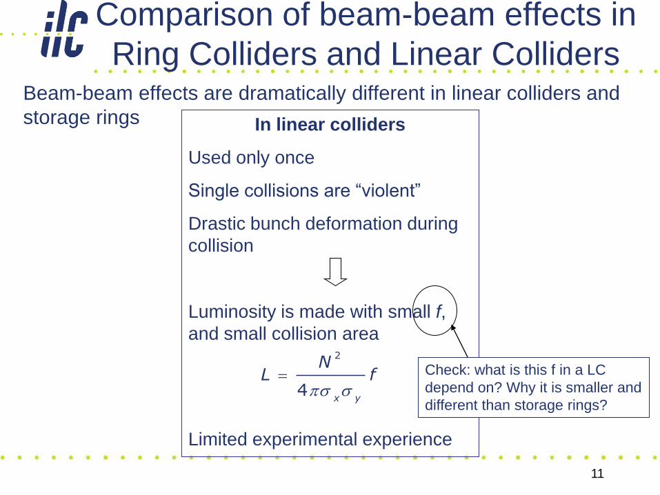
Comparison of beam-beam effects in
Ring Colliders and Linear CollidersBeam-beam effects are dramatically different in linear colliders and
storage rings In linear colliders
Used only once
Single collisions are “violent”
Drastic bunch deformation during
collision
Luminosity is made with small f,
and small collision area
Limited experimental experience
2
4x y
NL f
s s Check: what is this f in a LC
depend on? Why it is smaller and
different than storage rings?
12
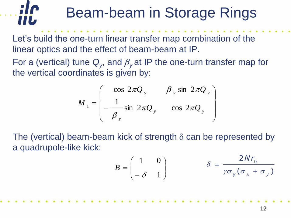
Beam-beam in Storage Rings
Let’s build the one-turn linear transfer map combination of the
linear optics and the effect of beam-beam at IP.
For a (vertical) tune Qy, and by at IP the one-turn transfer map for
the vertical coordinates is given by:
The (vertical) beam-beam kick of strength d can be represented by
a quadrupole-like kick:
yy
y
yyy
M
b
b
2cos2sin1
2sin2cos
1
1
01
dB
02
( )y x y
Nrd
gs s s
13
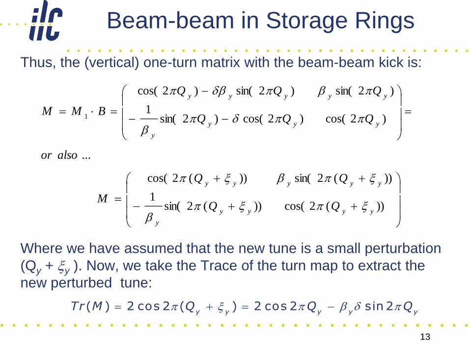
Beam-beam in Storage Rings
Thus, the (vertical) one-turn matrix with the beam-beam kick is:
Where we have assumed that the new tune is a small perturbation
(Qy + xy ). Now, we take the Trace of the turn map to extract the
new perturbed tune:
))(2cos())(2sin(1
))(2sin())(2cos(
...
)2cos()2cos()2sin(1
)2sin()2sin()2cos(
1
yyyy
y
yyyyy
yyy
y
yyyyy
M
alsoor
QQQ
QQQ
BMM
xxb
xbx
db
bdb
( ) 2 cos 2 ( ) 2 cos 2 sin 2y y y y y
Tr M Q Q Q x b d
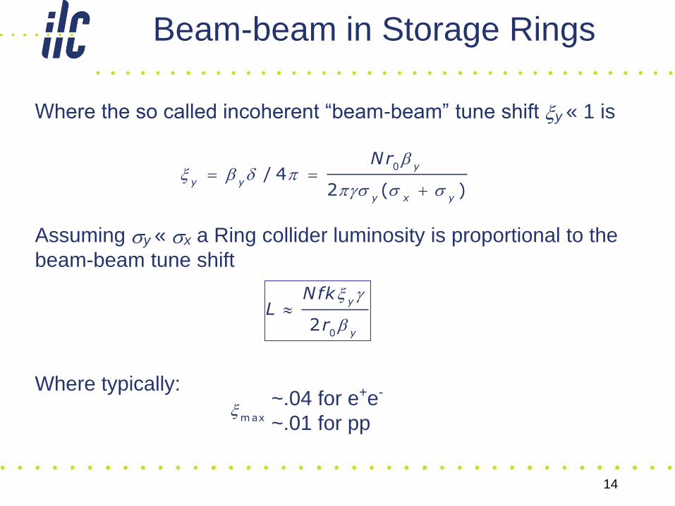
Where the so called incoherent “beam-beam” tune shift xy « 1 is
Assuming sy « sx a Ring collider luminosity is proportional to the
beam-beam tune shift
Where typically:
14
Beam-beam in Storage Rings
0/ 4
2 ( )
y
y y
y x y
Nr bx b d
gs s s
x g
b
02
y
y
NfkL
r
m axx
~.04 for e+e-
~.01 for pp
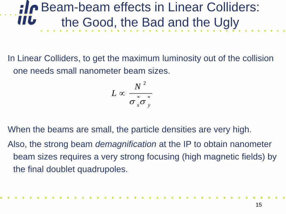
In Linear Colliders, to get the maximum luminosity out of the collision
one needs small nanometer beam sizes.
When the beams are small, the particle densities are very high.
Also, the strong beam demagnification at the IP to obtain nanometer
beam sizes requires a very strong focusing (high magnetic fields) by
the final doublet quadrupoles.
15
Beam-beam effects in Linear Colliders:
the Good, the Bad and the Ugly
**
2
yx
NL
ss
16
Beam-beam effects in Linear Colliders:
the Good, the Bad and the Ugly
High beam densities lead to the following good or bad beam-beam
effects:
• GOOD: Strong pinching effect of the bunches enhance luminosity
• BAD: Instability effects sets tight collision tolerances at IP
• BAD: high beamstrahlung radiation with luminosity spectrum dilution
• UGLY: pairs production, e+ e- generated by the radiation propagating
in the strong field of the bunches are source of Detector Background
17
Beam-beam effects in Linear Colliders:
the Good, the Bad and the Ugly
18
Beam-beam effects in linear Colliders:
the Good, the Bad and the Ugly
19
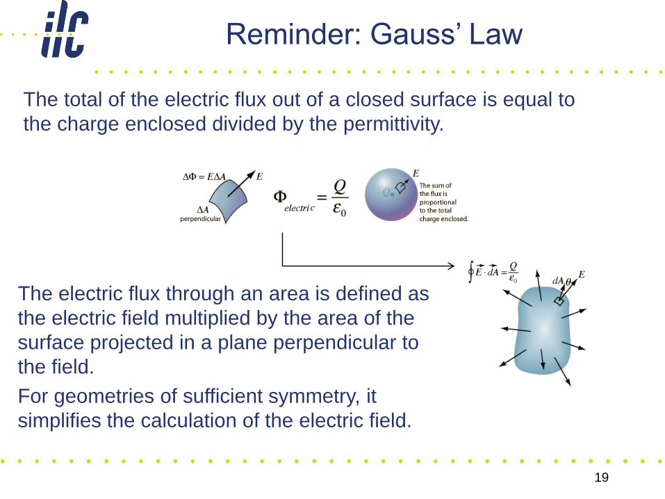
Reminder: Gauss’ Law
The total of the electric flux out of a closed surface is equal to
the charge enclosed divided by the permittivity.
The electric flux through an area is defined as
the electric field multiplied by the area of the
surface projected in a plane perpendicular to
the field.
For geometries of sufficient symmetry, it
simplifies the calculation of the electric field.
20
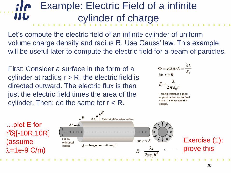
Example: Electric Field of a infinite
cylinder of charge
Let’s compute the electric field of an infinite cylinder of uniform
volume charge density and radius R. Use Gauss’ law. This example
will be useful later to compute the electric field for a beam of particles.
First: Consider a surface in the form of a
cylinder at radius r > R, the electric field is
directed outward. The electric flux is then
just the electric field times the area of the
cylinder. Then: do the same for r < R.
Exercise (1):
prove this
…plot E for
r[-10R,10R]
(assume
l=1e-9 C/m)
21
Electric and Magnetic fields in a beam
First we compute the Electric field E.
To compute the Electric field of a relativistic beam, we consider three
cases for the transverse beam charge distribution:
– Round Gaussian beam
– Flat Gaussian beam (exact)
– Flat Gaussian beam (approximation)
22
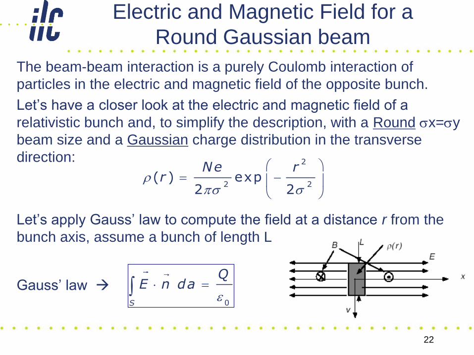
Electric and Magnetic Field for a
Round Gaussian beam
The beam-beam interaction is a purely Coulomb interaction of
particles in the electric and magnetic field of the opposite bunch.
Let’s have a closer look at the electric and magnetic field of a
relativistic bunch and, to simplify the description, with a Round sx=sy
beam size and a Gaussian charge distribution in the transverse
direction:
Let’s apply Gauss’ law to compute the field at a distance r from the
bunch axis, assume a bunch of length L
Gauss’ law
s s
2
2 2( ) exp
2 2
Ne rr
0
S
QE n da
e
23
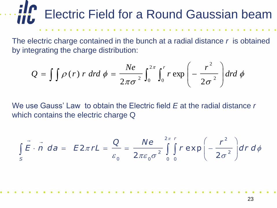
Electric Field for a Round Gaussian beam
The electric charge contained in the bunch at a radial distance r is obtained
by integrating the charge distribution:
We use Gauss’ Law to obtain the Electric field E at the radial distance r
which contains the electric charge Q
2 2
2 2
0 0 0 0
2 exp2 2
r
S
Q Ne rE n da E rL r dr d
fe e s s
fss
f
drdr
rNe
drdrrQr
2
0 0 2
2
22
exp2
)(
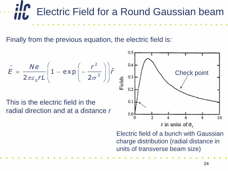
Finally from the previous equation, the electric field is:
This is the electric field in the
radial direction and at a distance r
24
e s
2
2
0
ˆ1 exp2 2
Ne rE r
rLCheck point
Electric Field for a Round Gaussian beam
Electric field of a bunch with Gaussian
charge distribution (radial distance in
units of transverse beam size)
25
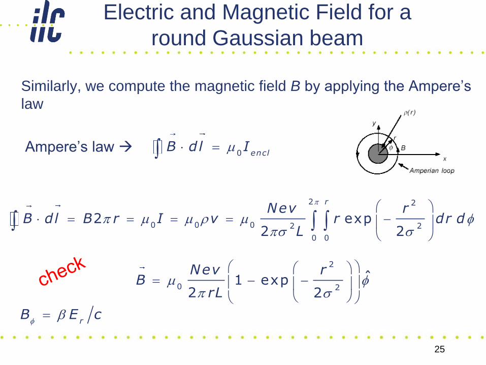
Electric and Magnetic Field for a
round Gaussian beam
Similarly, we compute the magnetic field B by applying the Ampere’s
law
Ampere’s law
2 2
0 0 0 2 2
0 0
2 exp2 2
rNev r
B dl B r I v r dr dL
fs s
f s
2
0 2ˆ1 exp
2 2
Nev rB
rL
0 enclB dl I
rB E c
fb
26
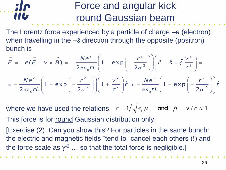
Force and angular kick
round Gaussian beam
The Lorentz force experienced by a particle of charge –e (electron)
when travelling in the –ŝ direction through the opposite (positron)
bunch is
where we have used the relations
This force is for round Gaussian distribution only.
[Exercise (2). Can you show this? For particles in the same bunch:
the electric and magnetic fields “tend to” cancel each others (!) and
the force scale as g-2 … so that the total force is negligible.]
fe s
e es s
2 2 2
2 2
0
2 2 2 2 2
2 2 2
0 0
ˆˆˆ( ) 1 exp2 2
ˆ ˆ1 exp 1 1 exp2 2 2
Ne r vF e E v B r s
rL c
Ne r v Ne rr r
rL rLc
1/100
cvc be and
27
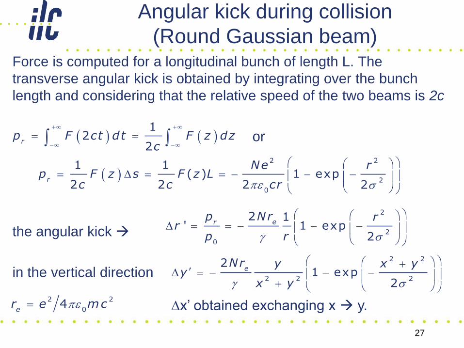
Angular kick during collision
(Round Gaussian beam)Force is computed for a longitudinal bunch of length L. The
transverse angular kick is obtained by integrating over the bunch
length and considering that the relative speed of the two beams is 2c
or
the angular kick
in the vertical direction
12
2rp F ct dt F z dz
c
e s
2 2
2
0
1 1( ) 1 exp
2 2 2 2r
Ne rp F z s F z L
c c cr
2
2
0
2 1' 1 exp
2
erNrp r
rp rg s
2 2
2 2 2
21 exp
2
eNr y x y
yx yg s
e2 2
04
er e mc x’ obtained exchanging x y.
28
Electric and Magnetic fields in a beam
First we compute the Electric field E.
To compute the Electric field of a relativistic beam, we consider three
cases for the transverse beam charge distribution:
– Round Gaussian beam
– Flat Gaussian beam (exact)
– Flat Gaussian beam (approximation)
29
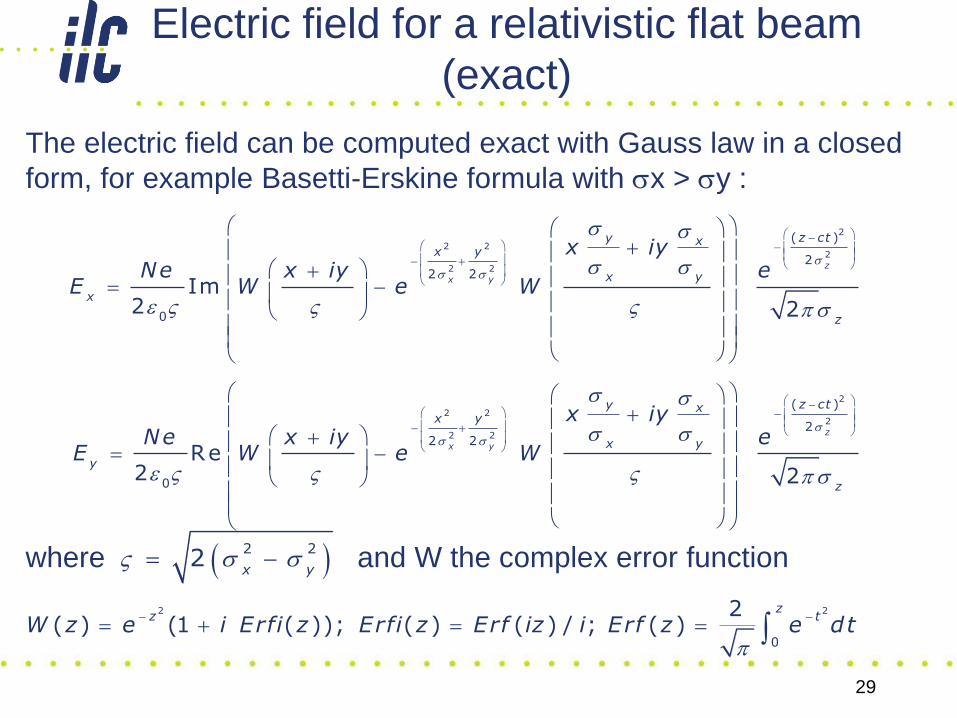
Electric field for a relativistic flat beam
(exact)
The electric field can be computed exact with Gauss law in a closed
form, for example Basetti-Erskine formula with sx > sy :
where and W the complex error function
2
2 22
2 2
( )
22 2
0
Re 2 2
z
x y
z cty xx y
x y
y
z
x iyNe x iy e
E W e W
ss s
s s
s s
e s
s s 2 2
2x y
2 2
0
2( ) (1 ( )); ( ) ( ) / ; ( )
zz t
W z e i Erfi z Erfi z Erf iz i Erf z e dt
2
2 22
2 2
( )
22 2
0
Im 2 2
z
x y
z cty xx y
x y
x
z
x iyNe x iy e
E W e W
ss s
s s
s s
e s
30
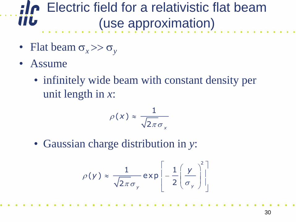
Electric field for a relativistic flat beam
(use approximation)
• Flat beam sx sy
• Assume
• infinitely wide beam with constant density per
unit length in x:
• Gaussian charge distribution in y:
s s
2
1 1( ) exp
22 yy
yy
s
1
( )2
x
x
31
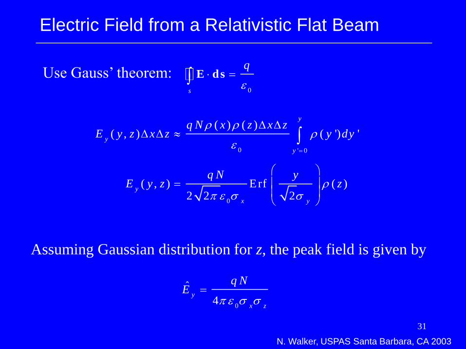
Electric Field from a Relativistic Flat Beam
0 ' 0
0
( ) ( )( , ) ( ') '
( , ) E rf ( )2 2 2
y
y
y
y
x y
q N x z x zE y z x z y dy
q N yE y z z
e
e s s
Use Gauss’ theorem:0s
q
e E ds
Assuming Gaussian distribution for z, the peak field is given by
0
ˆ
4y
x z
q NE
e s s
N. Walker, USPAS Santa Barbara, CA 2003
32
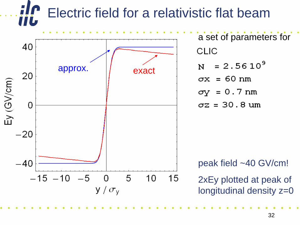
Electric field for a relativistic flat beam
peak field ~40 GV/cm!
2xEy plotted at peak of
longitudinal density z=0
exactapprox.
a set of parameters for
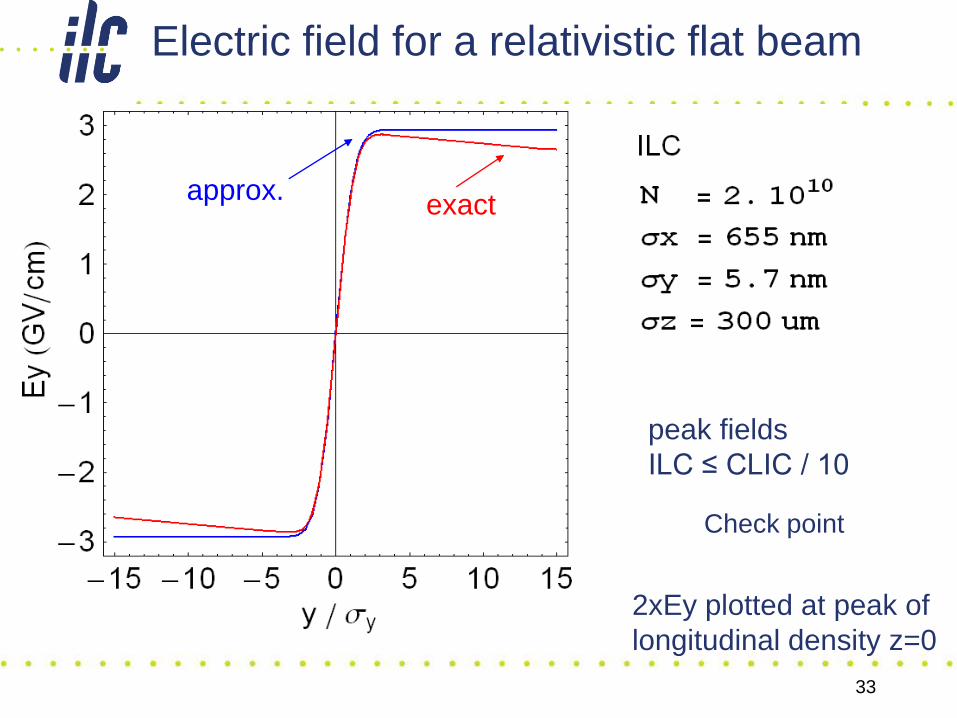
33
Electric field for a relativistic flat beam
exactapprox.
peak fields
ILC ≤ CLIC / 10
Check point
2xEy plotted at peak of
longitudinal density z=0
34
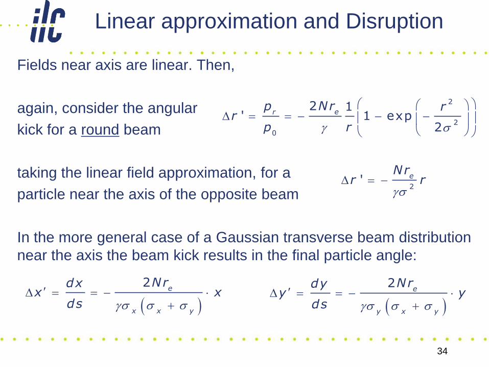
Linear approximation and Disruption
Fields near axis are linear. Then,
again, consider the angular
kick for a round beam
taking the linear field approximation, for a
particle near the axis of the opposite beam
In the more general case of a Gaussian transverse beam distribution
near the axis the beam kick results in the final particle angle:
2
2
0
2 1' 1 exp
2
erNrp r
rp rg s
2' e
Nrr r
gs
2e
y x y
Nrdyy y
ds gs s s
2e
x x y
Nrdxx x
ds gs s s
35
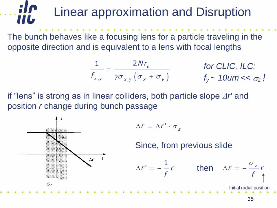
Linear approximation and Disruption
The bunch behaves like a focusing lens for a particle traveling in the
opposite direction and is equivalent to a lens with focal lengths
if “lens” is strong as in linear colliders, both particle slope r' and
position r change during bunch passage
, ,
21e
x y x y x y
Nr
f gs s s
for CLIC, ILC:
fy ~ 10um << sz !
zr r s
sz
1r r
f
zr rf
s
Since, from previous slide
then
Initial radial position
36
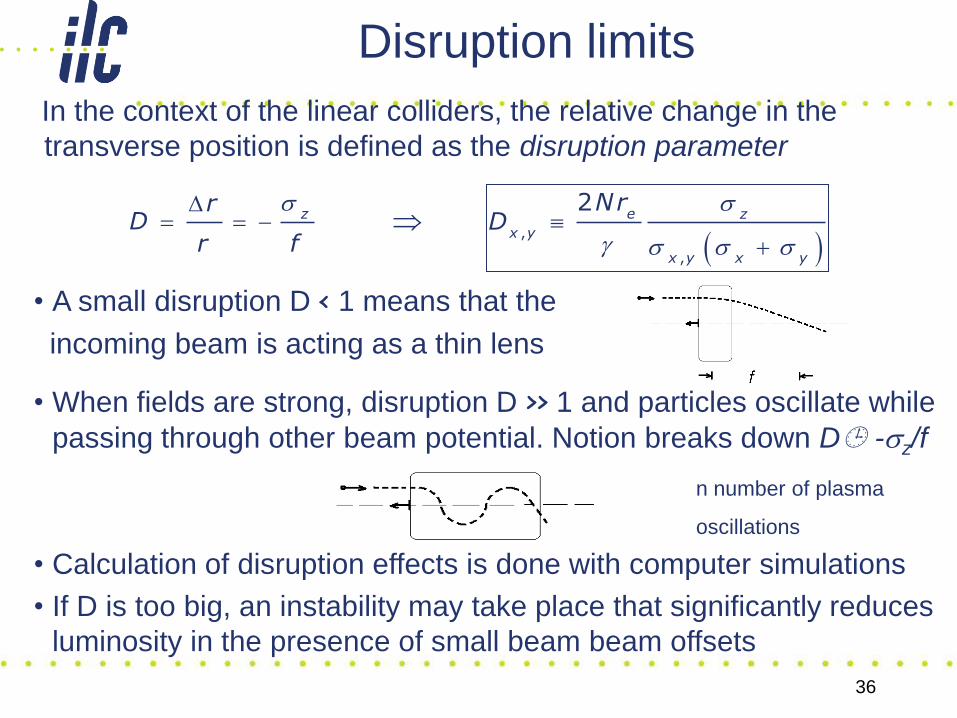
Disruption limits
• A small disruption D < 1 means that the
incoming beam is acting as a thin lens
• When fields are strong, disruption D >> 1 and particles oscillate while
passing through other beam potential. Notion breaks down D -sz/f
• Calculation of disruption effects is done with computer simulations
• If D is too big, an instability may take place that significantly reduces
luminosity in the presence of small beam beam offsets
n number of plasma
oscillations
In the context of the linear colliders, the relative change in the
transverse position is defined as the disruption parameter
,
,
2e z
x y
x y x y
NrD
s
g s s s
zr
Dr f
s
37
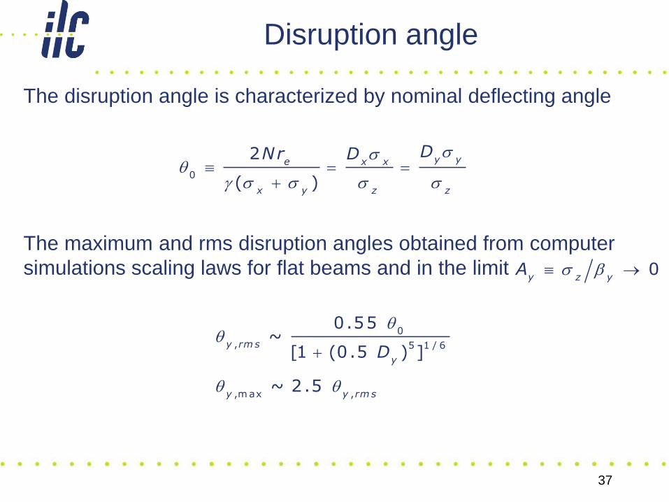
Disruption angle
The disruption angle is characterized by nominal deflecting angle
The maximum and rms disruption angles obtained from computer
simulations scaling laws for flat beams and in the limit
0
2
( )
y ye x x
x y z z
DNr D ssq
g s s s s
0
, 5 1 / 6
,m ax ,
0.55 ~
[1 (0.5 ) ]
~ 2.5
y rms
y
y y rms
D
q q
0y z yA s b
38
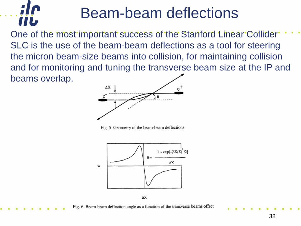
One of the most important success of the Stanford Linear Collider
SLC is the use of the beam-beam deflections as a tool for steering
the micron beam-size beams into collision, for maintaining collision
and for monitoring and tuning the transverse beam size at the IP and
beams overlap.
Beam-beam deflections
39
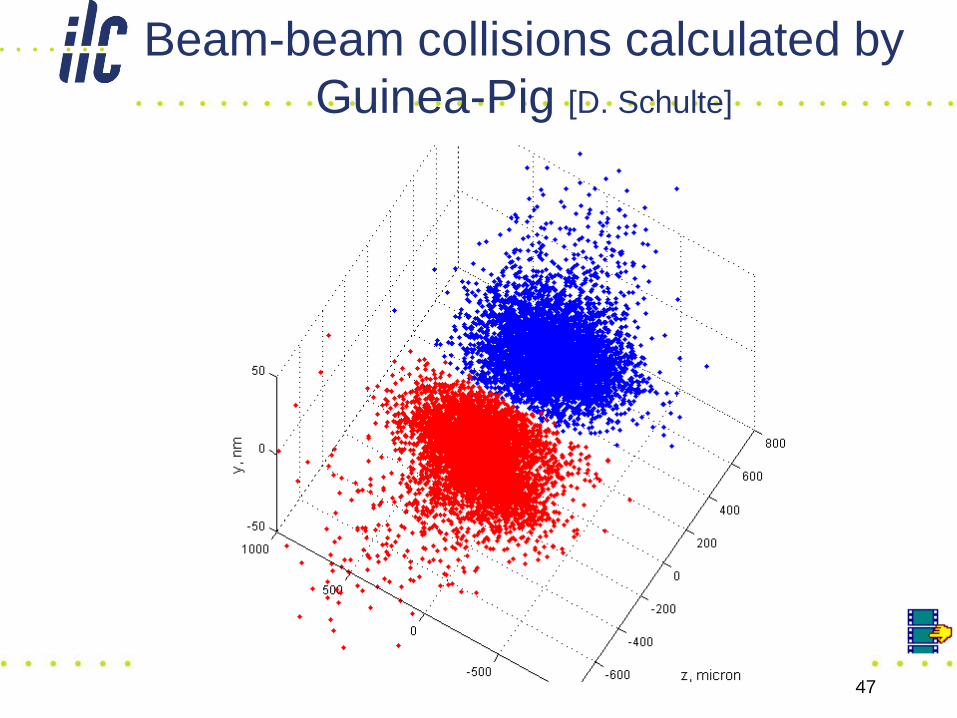
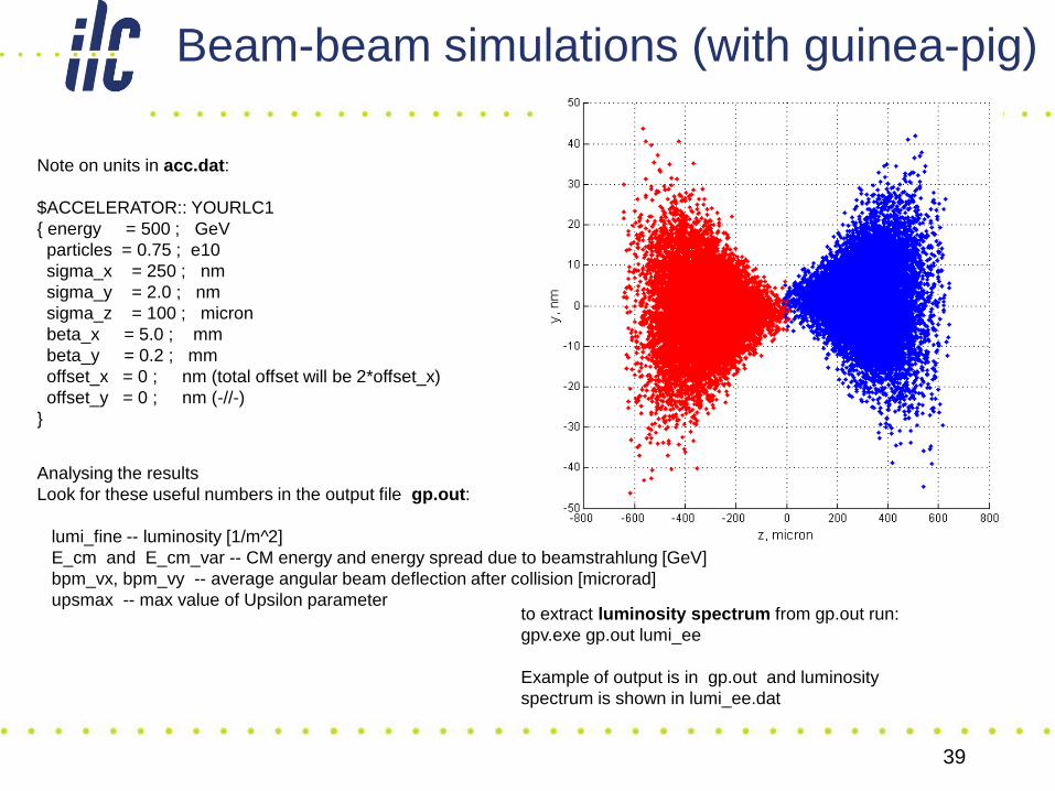
Beam-beam simulations (with guinea-pig)
Note on units in acc.dat:
$ACCELERATOR:: YOURLC1
{ energy = 500 ; GeV
particles = 0.75 ; e10
sigma_x = 250 ; nm
sigma_y = 2.0 ; nm
sigma_z = 100 ; micron
beta_x = 5.0 ; mm
beta_y = 0.2 ; mm
offset_x = 0 ; nm (total offset will be 2*offset_x)
offset_y = 0 ; nm (-//-)
}
Analysing the results
Look for these useful numbers in the output file gp.out:
lumi_fine -- luminosity [1/m^2]
E_cm and E_cm_var -- CM energy and energy spread due to beamstrahlung [GeV]
bpm_vx, bpm_vy -- average angular beam deflection after collision [microrad]
upsmax -- max value of Upsilon parameterto extract luminosity spectrum from gp.out run:
gpv.exe gp.out lumi_ee
Example of output is in gp.out and luminosity
spectrum is shown in lumi_ee.dat
January 22-26, 2007, Houston, Texas USPAS07 40
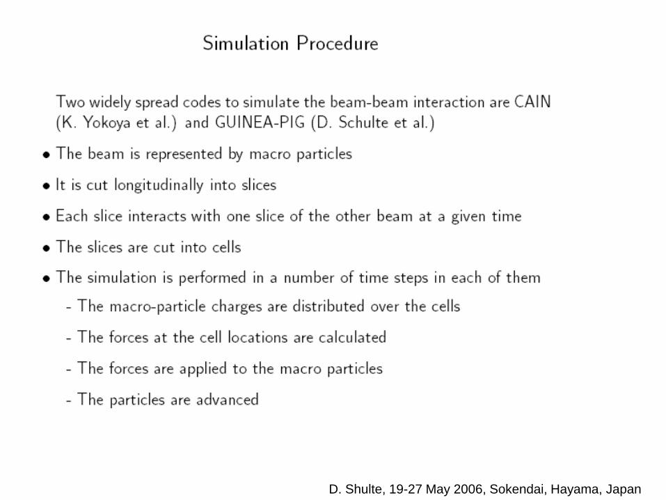
Simulations (with guinea-pig)
Selected
D. Shulte, 19-27 May 2006, Sokendai, Hayama, Japan
41
BEAM-BEAM
SIMULATIONS
42
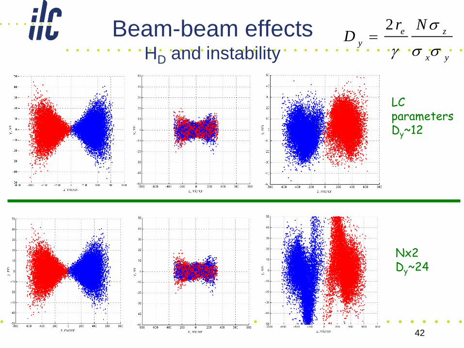
Beam-beam effectsHD and instability yx
ze
y
NrD
ss
s
g
2
LC parametersDy~12
Nx2Dy~24
43
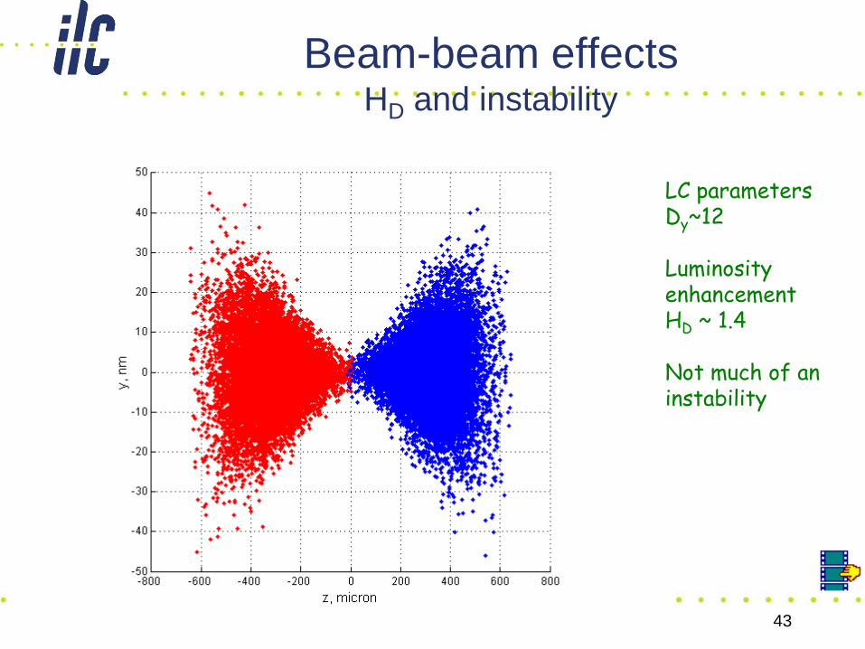
Beam-beam effectsHD and instability
LC parametersDy~12
Luminosity enhancement HD ~ 1.4
Not much of an instability
44
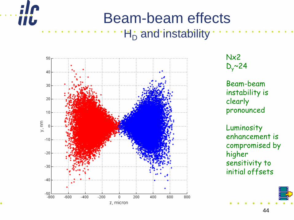
Beam-beam effectsHD and instability
Nx2Dy~24
Beam-beam instability is clearly pronounced
Luminosity enhancement is compromised by higher sensitivity to initial offsets
45
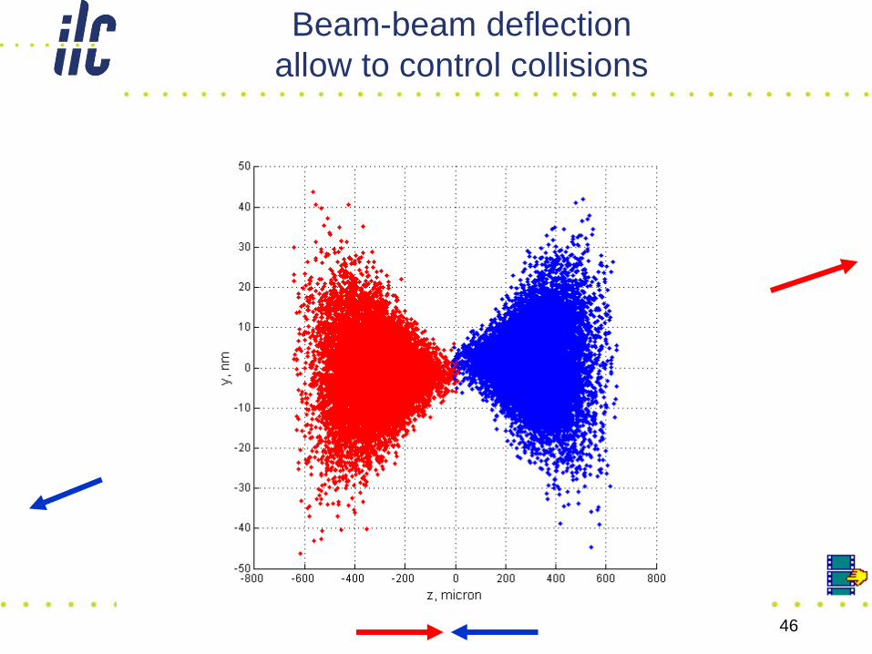
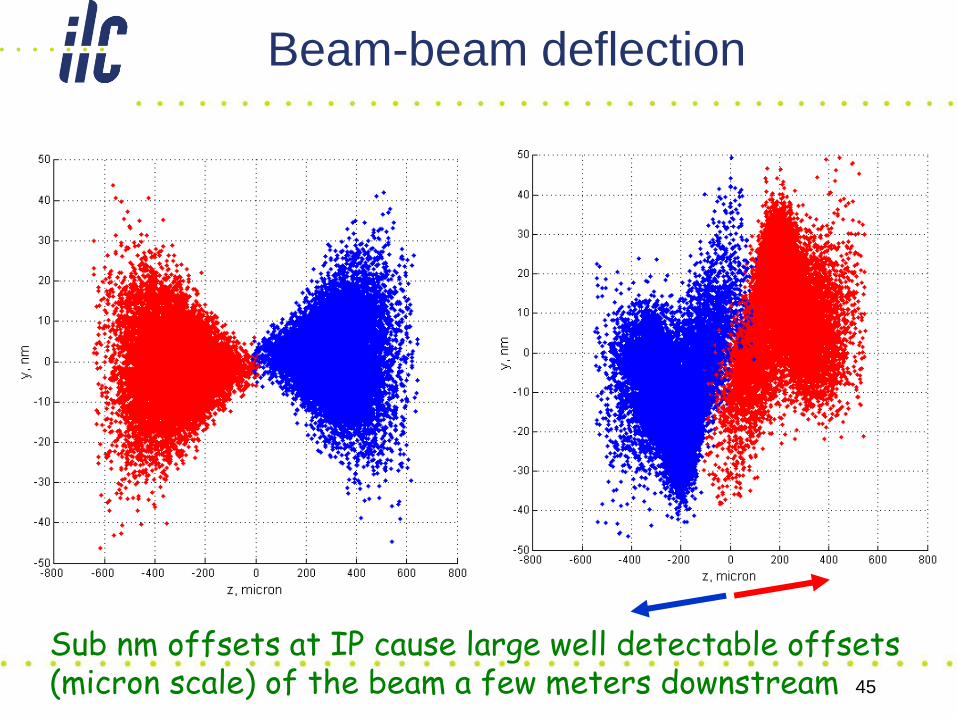
Beam-beam deflection
Sub nm offsets at IP cause large well detectable offsets (micron scale) of the beam a few meters downstream
48
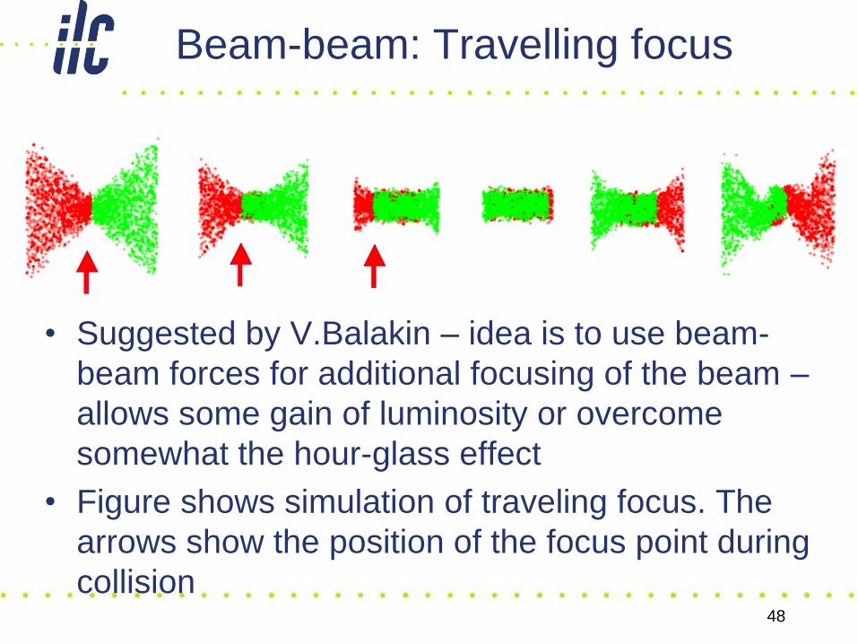
Beam-beam: Travelling focus
• Suggested by V.Balakin – idea is to use beam-
beam forces for additional focusing of the beam –
allows some gain of luminosity or overcome
somewhat the hour-glass effect
• Figure shows simulation of traveling focus. The
arrows show the position of the focus point during
collision
49
END OF FIRST
BEAM BEAM
LECTURE
50
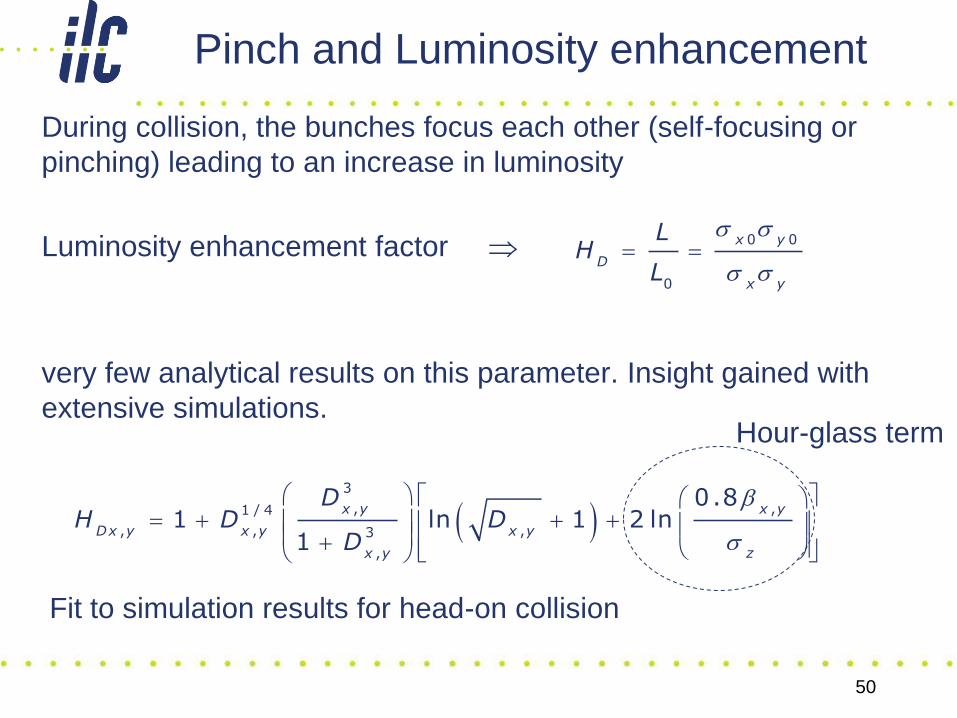
Pinch and Luminosity enhancement
During collision, the bunches focus each other (self-focusing or
pinching) leading to an increase in luminosity
Luminosity enhancement factor
very few analytical results on this parameter. Insight gained with
extensive simulations.
0 0
0
x y
D
x y
LH
L
s s
s s
3
, ,1 / 4
, , ,3
,
0.81 ln 1 2 ln
1
x y x y
Dx y x y x y
zx y
DH D D
D
b
s
Hour-glass term
Fit to simulation results for head-on collision
51
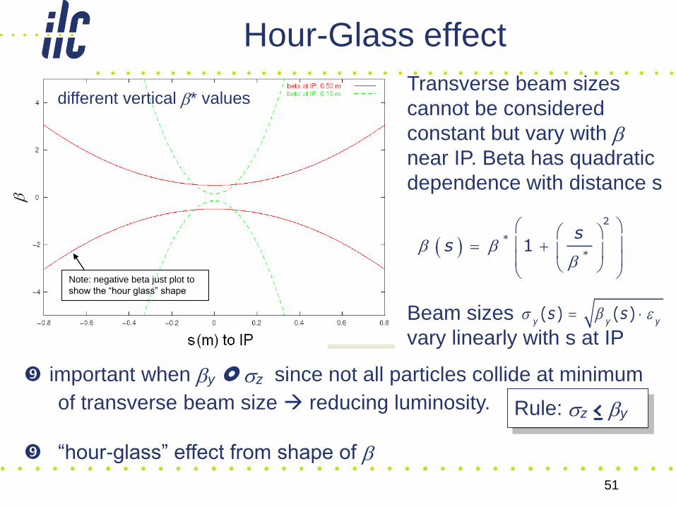
Hour-Glass effect
different vertical b* values Transverse beam sizes
cannot be considered
constant but vary with bnear IP. Beta has quadratic
dependence with distance s
Beam sizes
vary linearly with s at IP
2
*
*1
ssb b
b
important when by sz since not all particles collide at minimum
of transverse beam size reducing luminosity.
“hour-glass” effect from shape of b
Rule: sz ≤ by
( ) ( )y y ys ss b e
Note: negative beta just plot to
show the “hour glass” shape
52
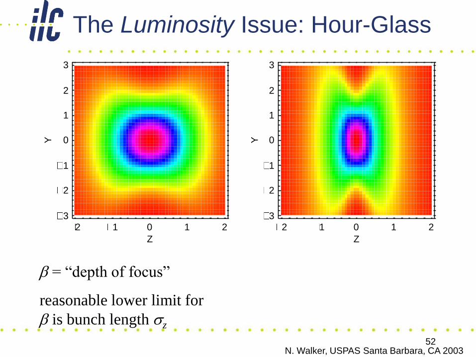
The Luminosity Issue: Hour-Glass
b = “depth of focus”
reasonable lower limit for
b is bunch length sz
2 1 0 1 2
Z
3
2
1
0
1
2
3
Y
2 1 0 1 2
Z
3
2
1
0
1
2
3
Y
N. Walker, USPAS Santa Barbara, CA 2003
53
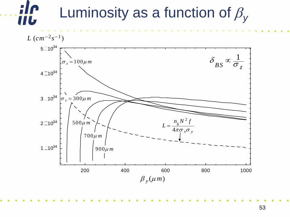
Luminosity as a function of by
200 400 600 800 1000
1 1034
2 1034
3 1034
4 1034
5 1034
300z ms
100z ms
500 m
700 m
900 m
( )y mb
2 1( )L cm s
2
4b
x y
n N fL
s s
1BS z
d s
54
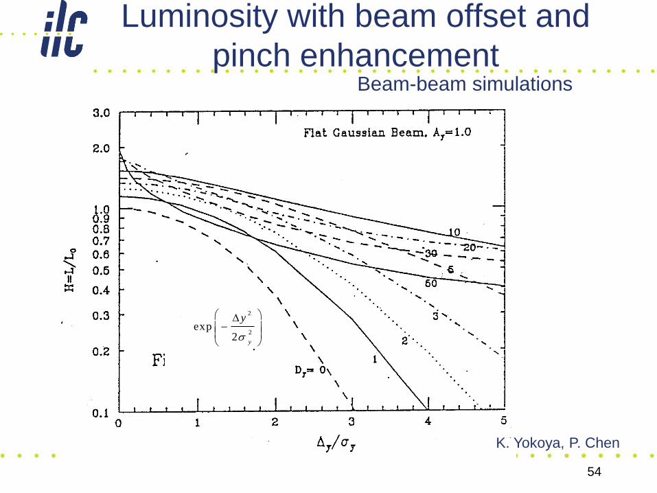
Luminosity with beam offset and
pinch enhancement
2
2exp
2s
y
y
Beam-beam simulations
K. Yokoya, P. Chen
55
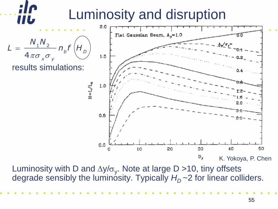
Luminosity and disruption
results simulations:
Luminosity with D and y/sy. Note at large D >10, tiny offsets degrade sensibly the luminosity. Typically HD ~2 for linear colliders.
K. Yokoya, P. Chen
1 2 4
b D
x y
N NL n f H
s s
56
Quantum Beamstrahlung
Particles accelerated transversely by the magnetic field of the
opposite bunch. In linear colliders:
• Magnetic fields reach kilo-Tesla!
• Longitudinal extent of the field is short sz~10-4, but emitted SR plays
crucial role in linear colliders
“Beamstrahlung” physics effects
• Spread in collision energy of e+e- Luminosity spectrum dilution
• Radiation interacts with beam fields to produce background e+e- and
+- pairs
1 beneficial effect Beamstrahlung used for diagnostics to keep
beams in collision
Exercise (3):
compute Bmax for CLIC beam
57
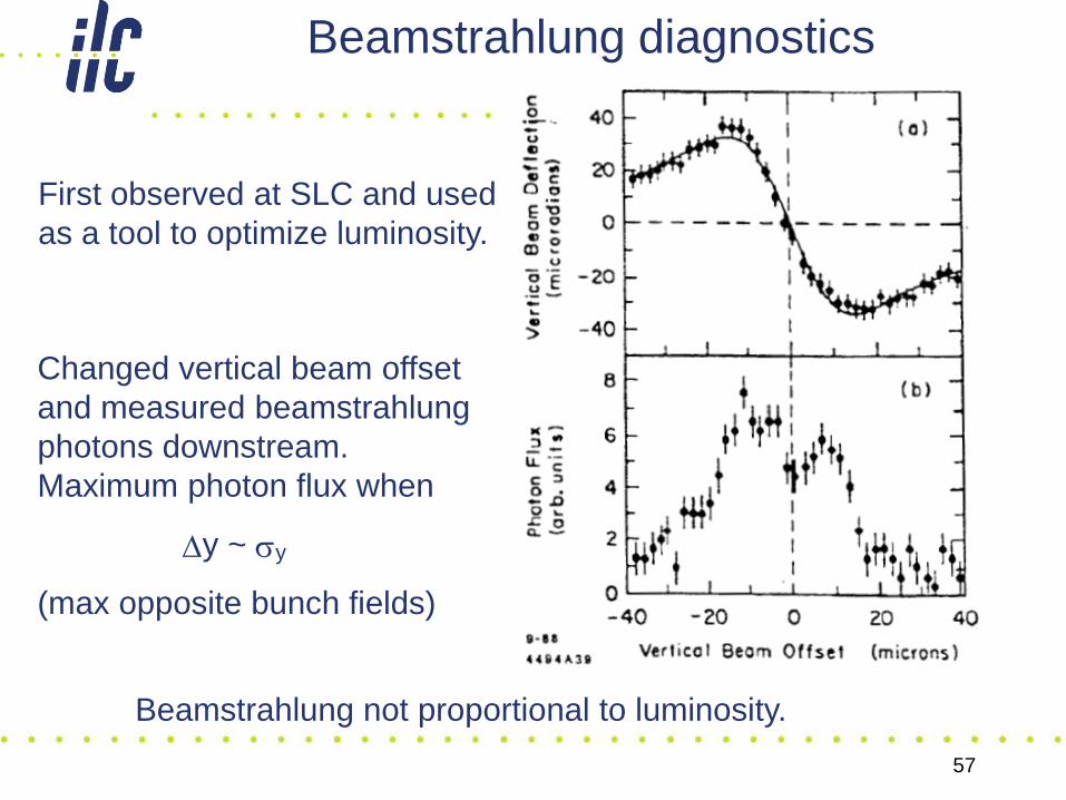
Beamstrahlung diagnostics
First observed at SLC and used
as a tool to optimize luminosity.
Changed vertical beam offset
and measured beamstrahlung
photons downstream.
Maximum photon flux when
y ~ sy
(max opposite bunch fields)
Beamstrahlung not proportional to luminosity.
58
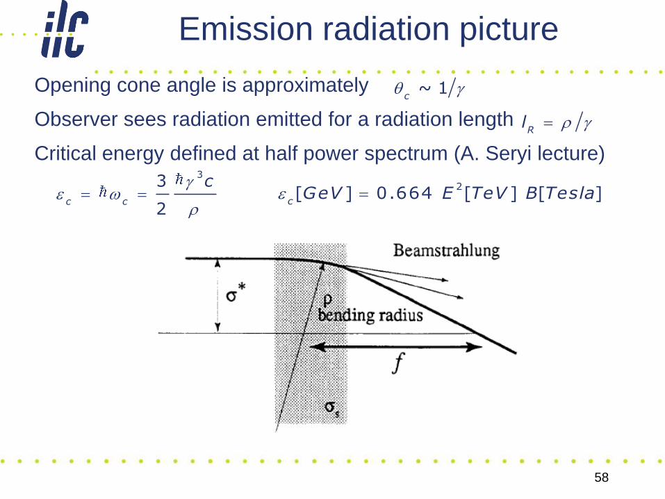
Emission radiation picture
Opening cone angle is approximately
Observer sees radiation emitted for a radiation length
Critical energy defined at half power spectrum (A. Seryi lecture)3
3
2c c
cge
~ 1c
q g
Rl g
2[ ] 0.664 [ ] [ ]cGeV E TeV B Teslae
59
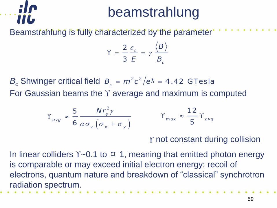
beamstrahlung
Beamstrahlung is fully characterized by the parameter
Bc Shwinger critical field
For Gaussian beams the average and maximum is computed
In linear colliders ~0.1 to 1, meaning that emitted photon energy
is comparable or may exceed initial electron energy: recoil of
electrons, quantum nature and breakdown of “classical” synchrotron
radiation spectrum.
2
3
c
c
B
E B
eg
2 24.42 GTesla
cB m c e
25
6
e
avg
z x y
Nr g
s s s
max
12
5avg
not constant during collision
60
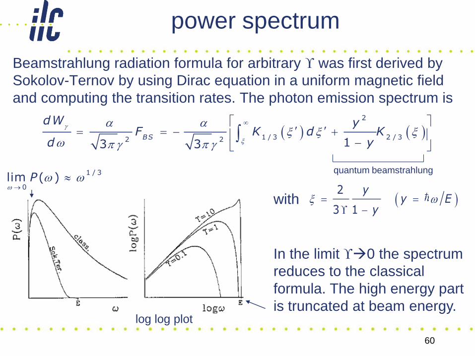
power spectrum
Beamstrahlung radiation formula for arbitrary was first derived by
Sokolov-Ternov by using Dirac equation in a uniform magnetic field
and computing the transition rates. The photon emission spectrum is
2
1 / 3 2 / 32 2 13 3BS
dW yF K d K
d y
g
x
x x x
g g
2
3 1
yy E
yx
1 / 3
0lim ( )P
quantum beamstrahlung
In the limit 0 the spectrum
reduces to the classical
formula. The high energy part
is truncated at beam energy.log log plot
with
61
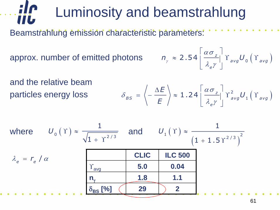
Luminosity and beamstrahlung
Beamstrahlung emission characteristic parameters:
approx. number of emitted photons
and the relative beam
particles energy loss
where and
02.54 z
avg avg
e
n Ug
s
l g
2
11.24 z
BS avg avg
e
EU
E
sd
l g
/e erl
02 / 3
1
1U
1 2
2 / 3
1
1 1.5
U
CLIC ILC 500
avg 5.0 0.04
ng 1.8 1.1
dBS [%] 29 2
62
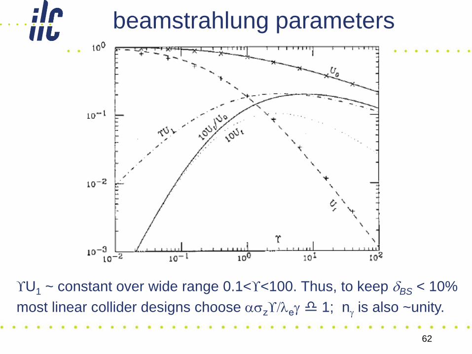
beamstrahlung parameters
U1 ~ constant over wide range 0.1<<100. Thus, to keep dBS < 10%
most linear collider designs choose sz/leg 1; ng is also ~unity.
January 22-26, 2007, Houston, Texas USPAS07 63
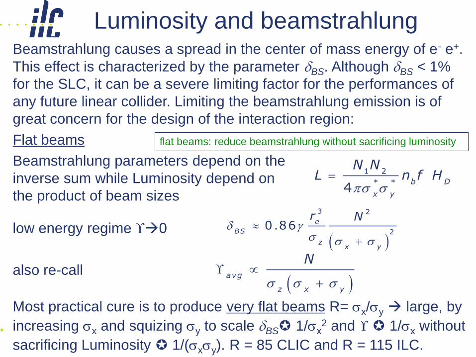
Luminosity and beamstrahlungBeamstrahlung causes a spread in the center of mass energy of e- e+.
This effect is characterized by the parameter dBS. Although dBS < 1%
for the SLC, it can be a severe limiting factor for the performances of
any future linear collider. Limiting the beamstrahlung emission is of
great concern for the design of the interaction region:
Flat beams
Beamstrahlung parameters depend on the
inverse sum while Luminosity depend on
the product of beam sizes
low energy regime 0
also re-call
Most practical cure is to produce very flat beams R= sx/sy large, by
increasing sx and squizing sy to scale dBS 1/sx2 and 1/sx without
sacrificing Luminosity 1/(sxsy). R = 85 CLIC and R = 115 ILC.
3 2
20.86 e
BS
zx y
r Nd g
s s s
avg
z x y
N
s s s
flat beams: reduce beamstrahlung without sacrificing luminosity
s s 1 2
* *
4b D
x y
N NL n f H
64
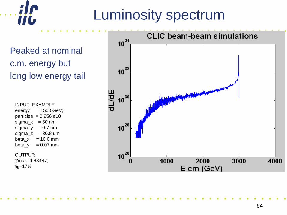
Luminosity spectrum
Peaked at nominal
c.m. energy but
long low energy tail
INPUT EXAMPLE
energy = 1500 GeV;
particles = 0.256 e10
sigma_x = 60 nm
sigma_y = 0.7 nm
sigma_z = 30.8 um
beta_x = 16.0 mm
beta_y = 0.07 mm
OUTPUT:
max=9.68447;
dE=17%
65
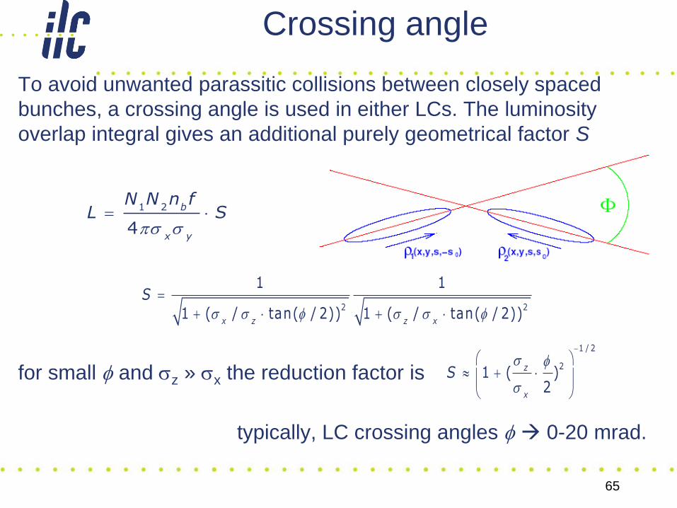
Crossing angle
To avoid unwanted parassitic collisions between closely spaced
bunches, a crossing angle is used in either LCs. The luminosity
overlap integral gives an additional purely geometrical factor S
for small f and sz » sx the reduction factor is
typically, LC crossing angles f 0-20 mrad.
1 2
4
b
x y
N N n fL S
s s
2 2
1 1
1 ( / tan( / 2)) 1 ( / tan( / 2))x z z x
Ss s f s s f
1 / 2
21 ( )
2
z
x
Ss f
s
66
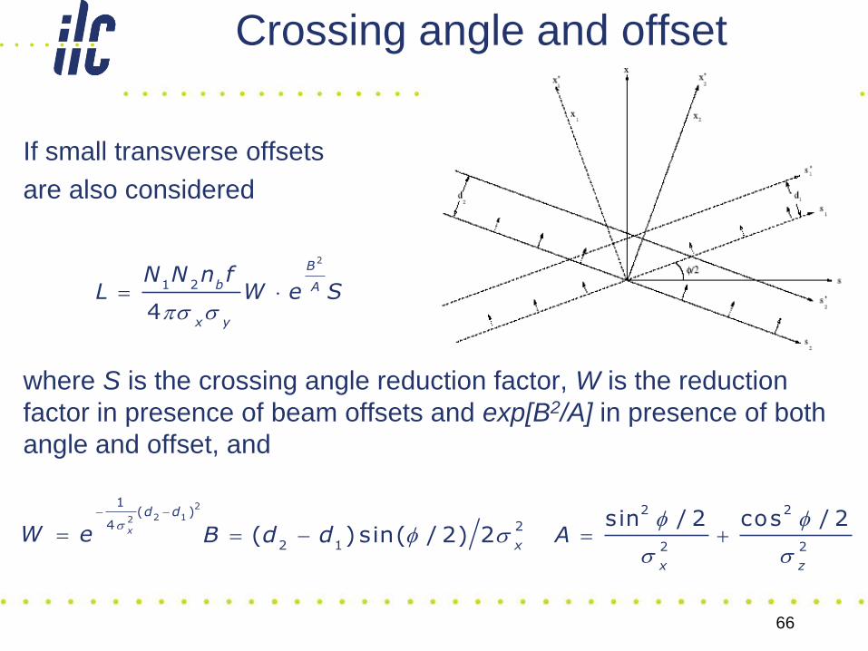
Crossing angle and offset
If small transverse offsets
are also considered
where S is the crossing angle reduction factor, W is the reduction
factor in presence of beam offsets and exp[B2/A] in presence of both
angle and offset, and
2
1 2
4
B
b A
x y
N N n fL W e S
s s
2
2 12
1( )
4 x
d d
W es
2
2 1( ) sin( / 2) 2
xB d d f s
2 2
2 2
sin / 2 cos / 2
x z
Af f
s s
67
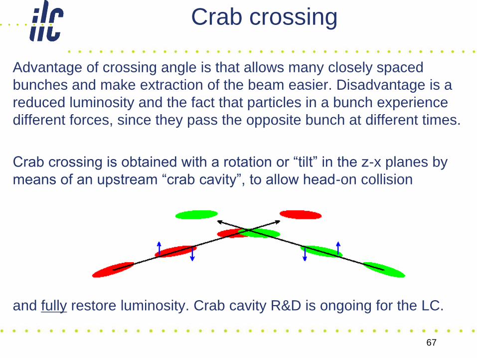
Crab crossing
Advantage of crossing angle is that allows many closely spaced
bunches and make extraction of the beam easier. Disadvantage is a
reduced luminosity and the fact that particles in a bunch experience
different forces, since they pass the opposite bunch at different times.
Crab crossing is obtained with a rotation or “tilt” in the z-x planes by
means of an upstream “crab cavity”, to allow head-on collision
and fully restore luminosity. Crab cavity R&D is ongoing for the LC.
68
Pair production
Production of e+e- pairs (see N. Mokhov lectures) is source of
detector background:
Incoherent process beamstrahlung “real” photons interact with oncoming electrons or positrons. Incoherent processes occur at low energies.
Coherent process photons propagating through the transverse electromagnetic field of the oncoming beam has a probability of turning into e+e- pairs. Contributed either by real or virtual photons.
69
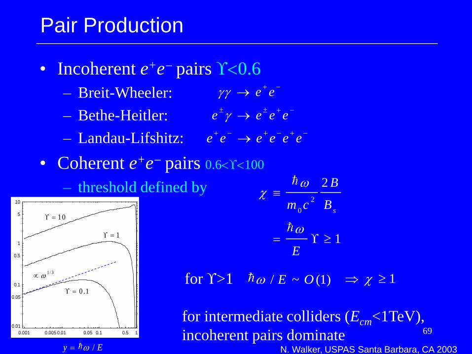
Pair Production
• Incoherent e+e pairs <0.6
– Breit-Wheeler:
– Bethe-Heitler:
– Landau-Lifshitz:
• Coherent e+e pairs 0.6<<100
– threshold defined by
e egg
e e e eg
e e e e e e
2
0
2
1
s
B
m c B
E
0.001 0.005 0.01 0.05 0.1 0.5 1
0.01
0.05
0.1
0.5
1
5
10
0 .1
1
10
1 / 3
/y E
for >1 / ~ (1)E O 1
for intermediate colliders (Ecm<1TeV),
incoherent pairs dominateN. Walker, USPAS Santa Barbara, CA 2003
70
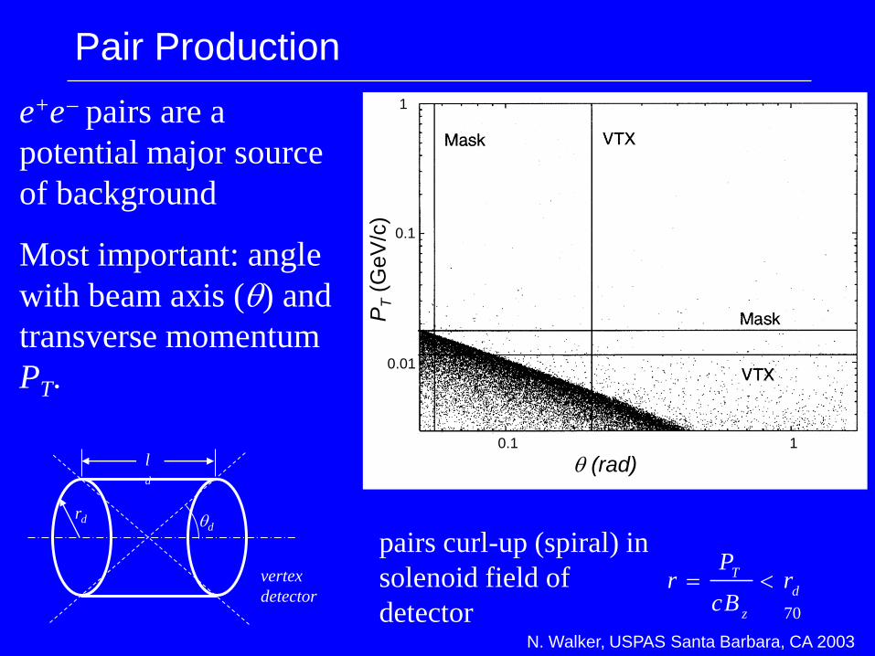
Pair Production
0.1 1
0.01
0.1
1
PT
(GeV
/c)
q (rad)
T
d
z
Pr r
cB <
pairs curl-up (spiral) in
solenoid field of
detector
rd
ld
qd
vertex
detector
e+e pairs are a
potential major source
of background
Most important: angle
with beam axis (q) and
transverse momentum
PT.
N. Walker, USPAS Santa Barbara, CA 2003
71
Many of these slides are based on previous contributions to
the field of beam-beam and beam delivery system
In particular, Thanks to:
N. Walker, D. Shulte, A. Seryi, K. Yokoya, P. Chen, K. Brown
and to many other colleagues …
72
References
Some references on beam-beam effects and final focus system:
[1] K. Yokoya and P. Chen, KEK Preprint 91-2
[2] N. Walker USPAS03 Lect. 1 and 7, Santa Barbara, CA
[3] D. Shulte ILC school Sokendai, Hayama, Japan May (2006)
[4] A. Seryi USPAS03 Santa Barbara
[5] L. Evans CAS84
[6] A. Chao, M. Tigner Handbook of Accel. Phys. And Eng.
[7] W. Herr and B. Muratori CAS03 CERN-2006-02
[8] E. Keil CAS95
[9] L. Rivkin CAS95
[10] G. Dugan USPAS02
[11] B. Siemann Luminosity and Beam Beam effects, Lect. 5, (1998)
[12] K. Oide Phys. Rev. Letter 61, 15, (1998)
[13] K. Brown SLAC-PUB-4811
[14] K. Brown, R. Sevranckx SLAC-PUB-3381
[15] P. Raimondi, A. Seryi Phys Rev. Letter86,3779 (2001)
73
Supplemental material
Feedback (keeping beam in collision)
Kink instability
Beam Beam Kick
Long Range Kink
banana beam
spent beam and exit angle
luminosity monitoring
74
1TeV
beam delivered
Nikolai Mokhov – Mauro Pivi – Andrei Seryi
e-e+ e- e-e+e+
Recommended