HAL Id: hal-01580251https://hal.archives-ouvertes.fr/hal-01580251
Submitted on 1 Sep 2017
HAL is a multi-disciplinary open accessarchive for the deposit and dissemination of sci-entific research documents, whether they are pub-lished or not. The documents may come fromteaching and research institutions in France orabroad, or from public or private research centers.
L’archive ouverte pluridisciplinaire HAL, estdestinée au dépôt et à la diffusion de documentsscientifiques de niveau recherche, publiés ou non,émanant des établissements d’enseignement et derecherche français ou étrangers, des laboratoirespublics ou privés.
Bare soil HYdrological balance model ”MHYSAN”:calibration and validation using SAR moisture productsand continuous thetaprobe network Measurements over
bare agricultural soils (Tunisia)Azza Gorrab, Vincent Simonneaux, Mehrez Zribi, S. Saadi, N. Baghdadi, Z.
Lili-Chabaane, Pascal Fanise
To cite this version:Azza Gorrab, Vincent Simonneaux, Mehrez Zribi, S. Saadi, N. Baghdadi, et al.. Bare soil HYdrologicalbalance model ”MHYSAN”: calibration and validation using SAR moisture products and continuousthetaprobe network Measurements over bare agricultural soils (Tunisia). Journal of Arid Environ-ments, Elsevier, 2017, 139, pp.11-25. �10.1016/j.jaridenv.2016.12.005�. �hal-01580251�
1
Bare Soil HYdrological Balance Model “MHYSAN”: Calibration and 1
Validation Using SAR Moisture Products and Continuous Thetaprobe 2
Network Measurements over bare agricultural soils (Tunisia) 3
Azza Gorrab 1,2,*, Vincent Simonneaux 2, Mehrez Zribi 2, Sameh Saadi 1,2, Nicolas Baghdadi 3, 4 Zohra Lili-Chabaane 1 and Pascal Fanise 2 5
1 Institut National Agronomique de Tunisie/Université de Carthage, 6 43 Avenue Charles Nicolle, 1082 Tunis Mahrajène, Tunisie; 7 E-Mails: [email protected] ; [email protected] 8
2 Centre d’Etudes Spatiales de la Biosphère, 18 Av. Edouard Belin, BP 2801, 9 31401 Toulouse Cedex 9, France; 10 E-Mails: [email protected] ; [email protected] ; [email protected] 11
3 IRTEA-UMR TETIS Maison de la télédétection, Montpellier, 34093, France ; 12 E-Mails : [email protected] 13
* Author to whom correspondence should be addressed; E-Mail: [email protected] ; 14
Tel.: +216-71-286-825; Fax: +216-71-750-254. 15
Abstract. The present study highlights the potential of multi-temporal X-band Synthetic Aperture 16
Radar (SAR) moisture products to be used for the calibration of a model reproducing soil moisture 17
(SM) variations. We propose the MHYSAN model (Modèle de bilan HYdrique des Sols Agricoles Nus) 18
for simulating soil water balance of bare soils. This model was used to simulate surface evaporation 19
fluxes and SM content at daily time scale over a semi-arid, bare agricultural site in Tunisia (North 20
Africa). Two main approaches are considered in this study. Firstly, the MHYSAN model was 21
successfully calibrated for seven sites using continuous thetaprobe measurements at two depths. Then 22
the possibility to extrapolate local SM simulations at distant sites, based on soil texture similarity only, 23
was tested. This extrapolation was assessed using SAR estimates and manual thetaprobe measurements 24
of SM recorded at these distant sites. The results reveal a bias of approximately 0.63% and 3.04%, and 25
an RMSE equal to 6.11% and 4.5%, for the SAR volumetric SM and manual thetaprobe measurements, 26
respectively. In a second approach, the MHYSAN model was calibrated using seven very high-27
resolution SAR (TerraSAR-X) SM outputs ranging over only two months. The simulated SM were 28
validated using continuous thetaprobe measurements during 15 months. Although the SM was measured 29
Author-produced version of the article published in : Journal of Arid Environments , vol. 139, 2017.p.11-25
2
on only seven different dates for the purposes of calibration, satisfactory results were obtained as a 30
result of the wide range of SM values recorded in these seven images. This led to good overall 31
calibration of the soil parameters, thus demonstrating the considerable potential of Sentinel-1 images for 32
daily soil moisture monitoring using simple models. 33
Keywords: Bare soil hydrological model, satellite soil moisture products, semi-arid area, continuous 34
soil moisture measurements. 35
1 Introduction 36
The conservation of water and soil resources is one of the main missions for sustainable agricultural 37
management. These natural resources are threatened by various types of degradation, such as water and 38
wind erosion, floods, drought and deforestation, all of which impede agricultural development. In recent 39
decades, the long periods of drought, especially in semi-arid regions, had a negative impact on available 40
water resources. In addition, most of the intercepted water is lost through evaporation, or by drainage, 41
deep percolation and subsurface runoff. Therefore, knowledge of water fluxes within the soil-42
atmosphere system is a major issue for the improvement of water use efficiency. Many studies have 43
been carried out to quantify these fluxes, and various tools have been developed to estimate the soil-44
water regime. These efforts can thus be expected to contribute to the sustainable management of natural 45
resources (Er-Raki et al., 2007; Gowda et al., 2008; Simonneaux et al., 2008; Zhang et al., 2010; Li et 46
al., 2009; Sutanto et al., 2012 and Saadi et al., 2015). 47
The amount of water stored in the soil is a crucial parameter, in situations where energy and mass fluxes 48
at the land surface-atmosphere boundary need to be determined, and is of fundamental importance to 49
many agricultural, hydrological, and meteorological processes (Koster et al., 2004; Seneviratne et al., 50
2010). Many soil water balance models have been developed, highlighting in particular the influence of 51
surface soil moisture conditions on the hydrological response of a watershed (Famiglietti and Wood, 52
1994; Entekhabi and Rodriguez-lturbe, 1994 ; Zehe and Bloschl, 2004; Brocca et al., 2005 and 2008; 53
Manfreda et al., 2005; Tramblay et al., 2012). Spatio-temporal soil moisture (SM) information is also of 54
Author-produced version of the article published in : Journal of Arid Environments , vol. 139, 2017.p.11-25
3
primary importance for the simulation of surface evaporation fluxes and vertical water circulation such 55
as surface water displacement via capillarity, and underground percolation. It is important for the 56
management of water resources, irrigation scheduling decisions, as well as the estimation of runoff and 57
soil erosion potential (Chen and Hu, 2004; Koster et al., 2004; Pandey et al., 2010; Bezerra et al., 2013; 58
Zhang et al., 2015). The spatial distribution of the soil's water content varies both vertically and 59
horizontally, as a consequence of variations in precipitation and evaporation, and the influences of 60
topography, soil texture, and vegetation. 61
As SM plays an important role in the hydrologic response, as well as land surface inputs to the 62
atmosphere, large spatio-temporal databases of moisture observation data need to be maintained, and 63
methodologies for the estimation of this key hydraulic property must be developed. This can be 64
achieved through the use of SM monitoring networks, providing frequent temporal observations at a 65
high spatial density. In situ station networks can be efficiently used as tools for the calibration of 66
hydrological models, and their interest has been demonstrated in various studies using different remote 67
sensing satellites and techniques (Wagner et al., 2008; Albergel et al., 2011; Gorrab et al., 2015b). 68
Considerable progress has been made in recent decades with the development of SM retrieval 69
techniques, based on the analysis of remotely sensed radar data. The high spatial resolution and regular 70
coverage provided by Imaging Synthetic Aperture Radar (SAR) sensors make these instruments a 71
promising additional source of data for the measurement of seasonal and long-term variations in surface 72
SM content, and could potentially improve hydrologic modeling applications (Baghdadi et al., 2008; 73
Barrett et al., 2009). Several algorithms have been developed to retrieve soil moisture from radar data 74
(Baghdadi et al., 2008; Zribi et al., 2011). In particular, the use of multi-temporal SAR acquisitions 75
allows SM to be effectively estimated, using a small number of assumptions, by analyzing changes in 76
radar backscattering over time (Zribi et al., 2005; Pathe et al., 2009; Gorrab et al., 2015b). 77
Subsequently, the integration of SM SAR products into hydrological balance models would be of 78
considerable interest, since it could provide scientists with the opportunity to improve hydrological 79
forecasting. Many recent studies have shown that the SM retrieved from SAR data generally agrees 80
Author-produced version of the article published in : Journal of Arid Environments , vol. 139, 2017.p.11-25
4
very well with that predicted by hydrological models (Baghdadi et al., 2007; Doubková et al., 2012; 81
Iacobellis et al., 2013; Santi et al., 2013; Pierdicca et al., 2014). Baghdadi et al., 2007, showed that the 82
monitoring of SM from SAR images was possible in operational phase. In fact, they compared 83
moistures simulated by the operational Météo-France ISBA soil-vegetation-atmosphere transfer model 84
with radar SM estimates to validate its pertinence. This comparison has shown an acceptable difference 85
between ISBA simulations and radar estimates. Pierdicca et al., 2014 compared SM values generated by 86
a soil water balance model with multi-temporal retrievals from ERS-1 images acquired over central 87
Italy. Very good results were obtained at the scale of the watershed, showing that the short three-day 88
revisit periodicity of ERS/SAR data can be used to compute relatively accurate estimations of the 89
temporal variations in SM. 90
SM remote sensing outputs can also be used for data assimilation and calibration in hydrological 91
transfer models, in order to evaluate their reliability (Weisse et al., 2003; Aubert et al., 2003; Qui et al., 92
2009; Brocca et al., 2010 and 2012; Draper et al., 2011; Renzullo et al., 2014; Massari et al., 2015; 93
Lievens et al., 2015; López López et al., 2016). For example, Aubert et al., 2003, integrated remotely 94
sensed SM data into their hydrological model, to improve the accuracy of their hydrological forecasts. 95
Their methodology involved the implementation of a sequential assimilation procedure, allowing step-96
by-step control of the model's successive outputs, thereby avoiding any divergence with respect to the 97
remotely sensed SM data. In a study published by (Brocca et al., 2010), a SM product derived from the 98
Advanced SCATterometer (ASCAT) sensor was introduced into a rainfall-runoff model (MISDc) and 99
applied to many sub-catchments of the Upper Tiber River in central Italy. The results reveal that even 100
with a coarse spatial resolution, remote sensing data can considerably improve the accuracy of runoff 101
predictions. 102
The growing availability of remote sensing SAR SM products, combined with the relatively large 103
number of parameters involved in soil water processes, means that moisture satellite data can now be 104
used for the calibration of distributed SM models. However, relatively few published studies have dealt 105
with the calibration of hydrological models using SAR SM products (François et al., 2003, Pauwels et 106
Author-produced version of the article published in : Journal of Arid Environments , vol. 139, 2017.p.11-25
5
al., 2002; Matgen et al., 2006; Montanari et al., 2009). In this context, the present study focuses mainly 107
on the effectiveness of high-resolution TerraSAR-X SM products to be used as calibration data in a 108
hydrological model. We propose a new, simple soil hydrological model called MHYSAN 109
(“Modelisation de Bilan HYdrique des Sols Agricoles Nus” in French, or "Water balance model for 110
bare agricultural soils") which was used to compute surface evaporation and water balance in central 111
Tunisia, thereby simulating soil moisture time series. Modeling bare soil behavior should be considered 112
as a first step toward agricultural soil moisture monitoring, but is all the more as bare soils represent the 113
majority of surface in our study area, like in most semi-arid areas. Our paper is organized in five 114
sections. The following section presents the database and ground station measurements used in this 115
study. Then, section 3 explains the functioning of the MHYSAN model and the calibration and 116
validation method. The results of the calibration and validation processes are presented and discussed in 117
Section 4, and then our conclusions and perspectives are provided in section 5. 118
2 Database description 119
2.1 Study Area Description 120
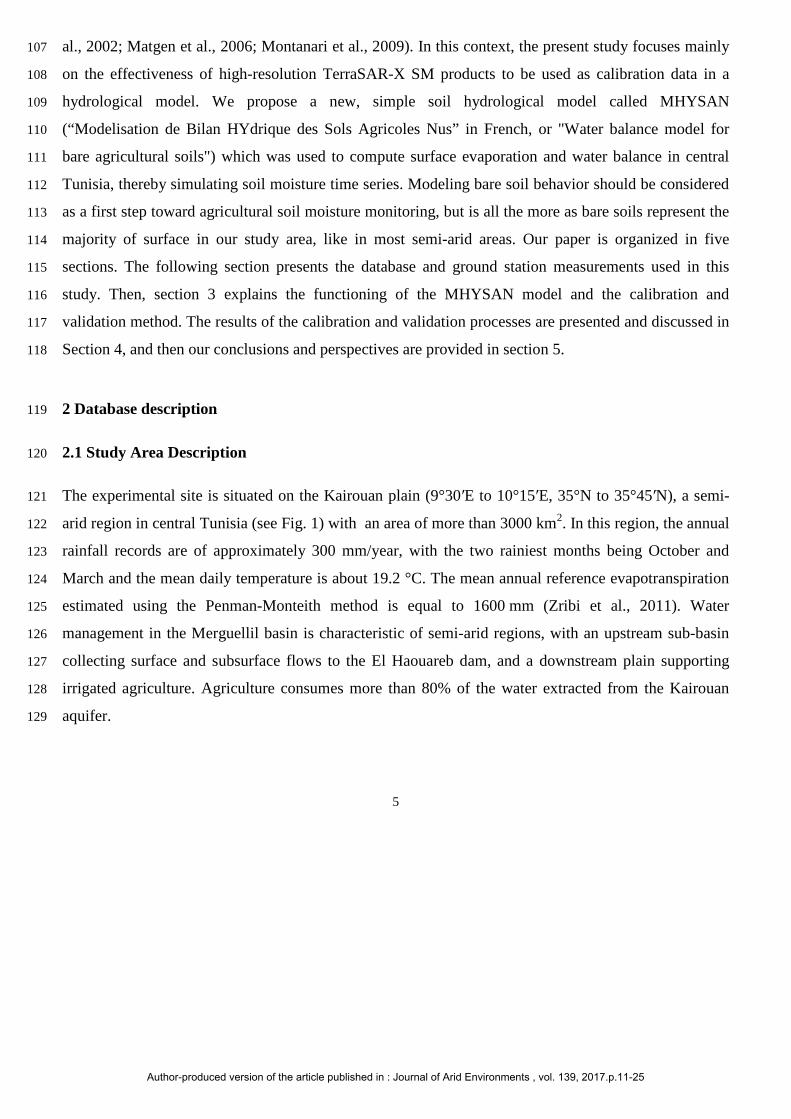
The experimental site is situated on the Kairouan plain (9°30′E to 10°15′E, 35°N to 35°45′N), a semi-121
arid region in central Tunisia (see Fig. 1) with an area of more than 3000 km2. In this region, the annual 122
rainfall records are of approximately 300 mm/year, with the two rainiest months being October and 123
March and the mean daily temperature is about 19.2 °C. The mean annual reference evapotranspiration 124
estimated using the Penman-Monteith method is equal to 1600 mm (Zribi et al., 2011). Water 125
management in the Merguellil basin is characteristic of semi-arid regions, with an upstream sub-basin 126
collecting surface and subsurface flows to the El Haouareb dam, and a downstream plain supporting 127
irrigated agriculture. Agriculture consumes more than 80% of the water extracted from the Kairouan 128
aquifer. 129
Author-produced version of the article published in : Journal of Arid Environments , vol. 139, 2017.p.11-25
6
130
Figure 1: Localization of the study site. 131
2.2 Ground and remote sensing database 132
2.2.1 Continuous in situ SM and meteorological data 133
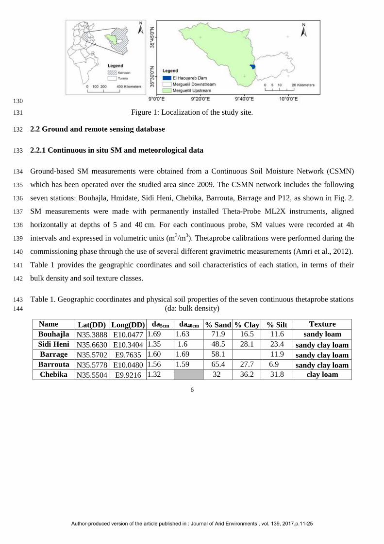
Ground-based SM measurements were obtained from a Continuous Soil Moisture Network (CSMN) 134
which has been operated over the studied area since 2009. The CSMN network includes the following 135
seven stations: Bouhajla, Hmidate, Sidi Heni, Chebika, Barrouta, Barrage and P12, as shown in Fig. 2. 136
SM measurements were made with permanently installed Theta-Probe ML2X instruments, aligned 137
horizontally at depths of 5 and 40 cm. For each continuous probe, SM values were recorded at 4h 138
intervals and expressed in volumetric units (m3/m3). Thetaprobe calibrations were performed during the 139
commissioning phase through the use of several different gravimetric measurements (Amri et al., 2012). 140
Table 1 provides the geographic coordinates and soil characteristics of each station, in terms of their 141
bulk density and soil texture classes. 142
Table 1. Geographic coordinates and physical soil properties of the seven continuous thetaprobe stations 143
(da: bulk density) 144
Name Lat(DD) Long(DD) da5cm da40cm % Sand % Clay % Silt Texture Bouhajl a N35.3888 E10.0477 1.69 1.63 71.9 16.5 11.6 sandy loam Sidi Heni N35.6630 E10.3404 1.35 1.6 48.5 28.1 23.4 sandy clay loam Barr age N35.5702 E9.7635 1.60 1.69 58.1
30311.9 sandy clay loam
Barrou ta N35.5778 E10.0480 1.56 1.59 65.4 27.7 6.9 sandy clay loam Chebika N35.5504 E9.9216 1.32 32 36.2 31.8 clay loam
Author-produced version of the article published in : Journal of Arid Environments , vol. 139, 2017.p.11-25
7
P12 N35.5563 E9.8716 1.47 69 18.5 13.5 sandy loam Hmidate N35.4757 E9.8449 1.67 81.1 12.7 6.2 sandy loam
145
Half-hourly measurements of solar radiation, air temperature and humidity, wind speed and rainfall 146
were recorded using two automated weather stations installed in the study area: Ben Salem and 147
Nasrallah (Fig. 2). 148
149
Figure 2: Locations of the continuous thetaprobe (green pins) and meteorological (yellow pins) stations 150
(courtesy of Google Earth). 151
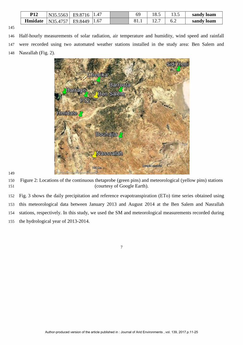
Fig. 3 shows the daily precipitation and reference evapotranspiration (ETo) time series obtained using 152
this meteorological data between January 2013 and August 2014 at the Ben Salem and Nasrallah 153
stations, respectively. In this study, we used the SM and meteorological measurements recorded during 154
the hydrological year of 2013-2014. 155
Author-produced version of the article published in : Journal of Arid Environments , vol. 139, 2017.p.11-25

8
(a) 156
(b) 157
Figure 3: Mean daily rainfall (red bars at the top) and reference evapotranspiration “ETo” (blue points) 158 recorded at two meteorological stations: (a) Nassrallah and (b) Ben Salem, for the hydrological year of 159
(2013-2014). 160
2.2.2 Analysis of SM and rainfall time series 161
The daily rainfall and SM variations for the 2013-2014 season were analyzed in order to check the 162
correlation between rainfall and soil moisture. Fig. 4 shows the example of the Chebika and Hmidate 163
probes. The rainfall gauges selected for each SM site were the closest to each of the continuous probe 164
0
20
40
60
80
100
1200
2
4
6
8
10
12
01/01/2013 20/02/2013 11/04/2013 31/05/2013 20/07/2013 08/09/2013 28/10/2013 17/12/2013 05/02/2014 27/03/2014 16/05/2014 05/07/2014
Ra
in (
mm
/da
y)
ETo
(m
m/d
ay
)
0
20
40
60
80
100
1200
2
4
6
8
10
12
01/01/2013 20/02/2013 11/04/2013 31/05/2013 20/07/2013 08/09/2013 28/10/2013 17/12/2013 05/02/2014 27/03/2014 16/05/2014 05/07/2014
Ra
in (
mm
/da
y)
ETo
(m
m/d
ay
)
Author-produced version of the article published in : Journal of Arid Environments , vol. 139, 2017.p.11-25
9
stations. The rainfall time series should be consistent with the temporal variations in SM recorded at the 165
depths of 5 cm and 40 cm. 166
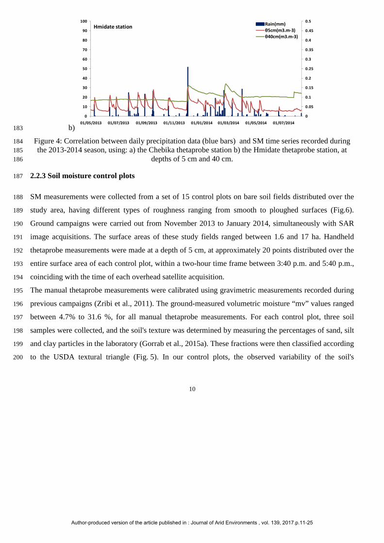
From Fig. 4, it can be seen that SM variations in the shallow layer (5 cm) are very different to those 167
observed in the deep layer (40 cm). The soil moisture content in both of these layers can be attributed 168
mainly to the influence of the soil's texture and pore size distribution (Bezerra et al., 2013; Zhang et al., 169
2015; Shabou et al., 2015). We also note that the deeper the probes are, the smoother the recorded 170
response. According to (Famiglietti et al., 1998; Amri et al., 2012), the amount of water stored in the 171
first centimeter of top soil increases rapidly in the presence rainfall, and can decrease significantly 172
within a few hours, due to atmospheric influences (evaporation …). This is the reason for which, as 173
shown in Fig. 4, the SM estimated at 40 cm is affected by considerably small variations than those 174
measured at the surface (5 cm). A large water content in the deep soil layers maintains an upward 175
vertical SM gradient, thereby contributing to the SM and evaporation observed in the shallow surface 176
layers (Chen and Hu, 2004). 177
Overall, the precipitation inputs are quite well correlated with the observed SM variations, in particular 178
the surface SM (θ5cm). For the 2013-2014 period, small discrepancies are occasionally observed between 179
SM and precipitation, since rainfall events are not always accompanied by an increase in SM, and some 180
SM variations are not correlated with any rainfall event. 181
a) 182
0
0.05
0.1
0.15
0.2
0.25
0.3
0.35
0.4
0.45
0.5
0
10
20
30
40
50
60
70
80
90
100
01/05/2013 01/07/2013 01/09/2013 01/11/2013 01/01/2014 01/03/2014 01/05/2014
Chebika StationRain(mm)
θ5cm(m3.m-3)
θ40cm(m3.m-3)
Author-produced version of the article published in : Journal of Arid Environments , vol. 139, 2017.p.11-25
10
b) 183
Figure 4: Correlation between daily precipitation data (blue bars) and SM time series recorded during 184 the 2013-2014 season, using: a) the Chebika thetaprobe station b) the Hmidate thetaprobe station, at 185
depths of 5 cm and 40 cm. 186
2.2.3 Soil moisture control plots 187
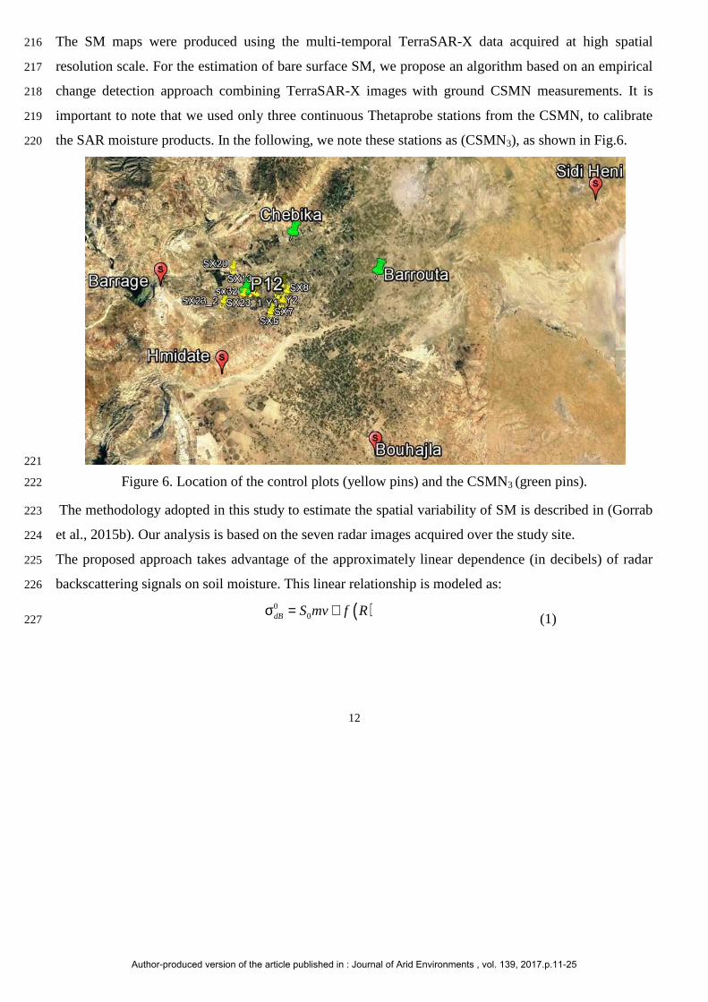
SM measurements were collected from a set of 15 control plots on bare soil fields distributed over the 188
study area, having different types of roughness ranging from smooth to ploughed surfaces (Fig.6). 189
Ground campaigns were carried out from November 2013 to January 2014, simultaneously with SAR 190
image acquisitions. The surface areas of these study fields ranged between 1.6 and 17 ha. Handheld 191
thetaprobe measurements were made at a depth of 5 cm, at approximately 20 points distributed over the 192
entire surface area of each control plot, within a two-hour time frame between 3:40 p.m. and 5:40 p.m., 193
coinciding with the time of each overhead satellite acquisition. 194
The manual thetaprobe measurements were calibrated using gravimetric measurements recorded during 195
previous campaigns (Zribi et al., 2011). The ground-measured volumetric moisture “mv” values ranged 196
between 4.7% to 31.6 %, for all manual thetaprobe measurements. For each control plot, three soil 197
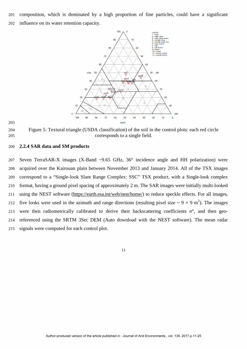
samples were collected, and the soil's texture was determined by measuring the percentages of sand, silt 198
and clay particles in the laboratory (Gorrab et al., 2015a). These fractions were then classified according 199
to the USDA textural triangle (Fig. 5). In our control plots, the observed variability of the soil's 200
0
0.05
0.1
0.15
0.2
0.25
0.3
0.35
0.4
0.45
0.5
0
10
20
30
40
50
60
70
80
90
100
01/05/2013 01/07/2013 01/09/2013 01/11/2013 01/01/2014 01/03/2014 01/05/2014 01/07/2014
Hmidate station Rain(mm)
θ5cm(m3.m-3)
θ40cm(m3.m-3)
Author-produced version of the article published in : Journal of Arid Environments , vol. 139, 2017.p.11-25
11
composition, which is dominated by a high proportion of fine particles, could have a significant 201
influence on its water retention capacity. 202
203
Figure 5: Textural triangle (USDA classification) of the soil in the control plots: each red circle 204
corresponds to a single field. 205
2.2.4 SAR data and SM products 206
Seven TerraSAR-X images (X-Band ~9.65 GHz, 36° incidence angle and HH polarization) were 207
acquired over the Kairouan plain between November 2013 and January 2014. All of the TSX images 208
correspond to a “Single-look Slant Range Complex: SSC” TSX product, with a Single-look complex 209
format, having a ground pixel spacing of approximately 2 m. The SAR images were initially multi-looked 210
using the NEST software (https://earth.esa.int/web/nest/home/) to reduce speckle effects. For all images, 211
five looks were used in the azimuth and range directions (resulting pixel size ~ 9 × 9 m2). The images 212
were then radiometrically calibrated to derive their backscattering coefficients σ°, and then geo-213
referenced using the SRTM 3Sec DEM (Auto download with the NEST software). The mean radar 214
signals were computed for each control plot. 215
Author-produced version of the article published in : Journal of Arid Environments , vol. 139, 2017.p.11-25
12
The SM maps were produced using the multi-temporal TerraSAR-X data acquired at high spatial 216
resolution scale. For the estimation of bare surface SM, we propose an algorithm based on an empirical 217
change detection approach combining TerraSAR-X images with ground CSMN measurements. It is 218
important to note that we used only three continuous Thetaprobe stations from the CSMN, to calibrate 219
the SAR moisture products. In the following, we note these stations as (CSMN3), as shown in Fig.6. 220
221
Figure 6. Location of the control plots (yellow pins) and the CSMN3 (green pins). 222
The methodology adopted in this study to estimate the spatial variability of SM is described in (Gorrab 223
et al., 2015b). Our analysis is based on the seven radar images acquired over the study site. 224
The proposed approach takes advantage of the approximately linear dependence (in decibels) of radar 225
backscattering signals on soil moisture. This linear relationship is modeled as: 226
( )00dB S mv f Rσ = +
(1) 227
Author-produced version of the article published in : Journal of Arid Environments , vol. 139, 2017.p.11-25
13
where S0 is the radar signal’s sensitivity to soil moisture (mv), and f(R) is a function of the roughness R. 228
The change in soil moisture ∆mv between two successive TerraSAR-X image acquisitions (11 day 229
period in the case of the present study), can be expressed as: 230
∆�� = ∆�°�∆�()� (2) 231
where ∆σ° is the radar signal difference, obtained by subtracting consecutive radar backscatter images 232
acquired over a given area (i.e. the change in signal strength between two acquisition dates), and ∆f(R) is 233
the difference in radar signal resulting from roughness contributions, between two successive radar 234
images. 235
The proposed algorithms are validated by comparing the radar estimations with ground-truth 236
measurements made in control plots, characterized by soil moistures ranging between dry and wet 237
conditions. Since a small improvement in the soil moisture estimation accuracy is observed when the 238
roughness variations are taken into account, the resulting soil moisture maps are computed for each date 239
dt and each pixel (i, j), as: 240
( ) ( ) ( )11 ,,,,,,, −− +∆= tvttvtv djimddjimdjim (3) 241
where ��(�, �, ��) is the SM at pixel (i,j) and date dt , ��(�, �, ����) is the SM at pixel (i,j) and date dt-1, 242
and ∆��(�, �, ��, ����) is the change in SM at pixel (i,j), between the dates ��, ����. 243
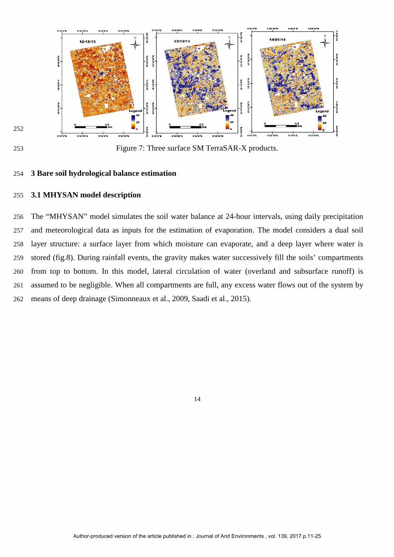
Fig. 7 shows three bare soil moisture maps computed using the above algorithm on three different dates: 244
*12/12/2013: was a dry date, and the spatial variations in soil moisture can be seen to be low. 245
*23/12/2013: was the wettest day (the recorded precipitation was approximately 38.6 mm), and the 246
spatial variations in soil moisture are relatively homogenous (dark blue) 247
*14/01/2014: was characterized by medium values of soil moisture and highly heterogeneous levels of 248
soil moisture (dark blue to light). 249
The TerraSAR-X SM maps provided data representing the volumetric soil moisture content expressed 250
in volumetric percentage units (vol. %). 251
Author-produced version of the article published in : Journal of Arid Environments , vol. 139, 2017.p.11-25
14
252
Figure 7: Three surface SM TerraSAR-X products. 253
3 Bare soil hydrological balance estimation 254
3.1 MHYSAN model description 255
The “MHYSAN” model simulates the soil water balance at 24-hour intervals, using daily precipitation 256
and meteorological data as inputs for the estimation of evaporation. The model considers a dual soil 257
layer structure: a surface layer from which moisture can evaporate, and a deep layer where water is 258
stored (fig.8). During rainfall events, the gravity makes water successively fill the soils’ compartments 259
from top to bottom. In this model, lateral circulation of water (overland and subsurface runoff) is 260
assumed to be negligible. When all compartments are full, any excess water flows out of the system by 261
means of deep drainage (Simonneaux et al., 2009, Saadi et al., 2015). 262
Author-produced version of the article published in : Journal of Arid Environments , vol. 139, 2017.p.11-25

15
263
Figure 8: Schematic representation of the conceptual bare soil hydrological model “MHYSAN”. 264
Ze [mm] is the height of the evaporative layer. Below this surface layer, a deep layer of height Zd [mm] 265
is modeled. TEW is the water column [mm] representing the difference between the moisture content at 266
field capacity and the residual water content that cannot be evaporated from the soil, and is described by 267
the following expression Eq. (1): 268
��� = �θ��– ���� ∗ "�, (1) 269
The evaporative capacity of the deep compartment (TDW) is computed in a similar manner to the TEW, 270
using the following expression Eq. (2): 271
�#� = (θ�� − θ���) ∗ "� (2) 272
Capillary processes are also modeled in MHYSAN, either upwards or downwards, between the 273
evaporative layer and the deep compartment, on the basis of their relative water contents. In particular, 274
this allows evaporation to continue long after a rainfall event, since the deeper layers can sustain low 275
evaporation fluxes at the surface. The daily amount of water diffusing between the two layers, Dif ed, is 276
computed following Eq. (3): 277
Author-produced version of the article published in : Journal of Arid Environments , vol. 139, 2017.p.11-25
16
#��%& = ���� ∗ '(()*+),,-)., �((/*+)0,-).0
θ12 3, (3) 278
where De,i and Dd,i represent the depletion of water in the evaporation and deep layers for day i (i.e. the 279
volume of voids as compared to soil at field capacity), and cdif is the diffusion coefficient [mm·day−1]. 280
The MHYSAN model balances the soil's daily water budget by ensuring that water inputs and outputs 281
are conserved, in accordance with the following expression Eq. (4): 282
�4 + #64 + 78�4 =64 (4) 283
with: 284
Ei Evaporation 285
DPi Deep Percolation (drainage) 286
∆SWi Variation of the soil's water content 287
Pi Precipitation 288
The evaporation (Ei) from a bare soil surface is defined as the volume of water vapor removed from the 289
soil's surface and transferred to the atmosphere and is estimated using the FAO-56 formalism (Allen et 290
al., 1998) using equation 5: 291
�4 = 9%,4 ∗ ��:, (5) 292
Where 293
ETo is the grass reference evapotranspiration (mm/day). This term was computed using the expressions 294
proposed by Allen et al. (1998), where Ke,i is the evaporation coefficient, related to the volume of 295
water in the surface layer, obtained with equation 6: 296
9%,4 = (;<=�>0,-)(;<=�?/) ≤ 1, (6) 297
and RE is the coefficient of resistance to evaporation. 298
The depletion (De,i) is updated every day from the soil water balance as follows: 299
Author-produced version of the article published in : Journal of Arid Environments , vol. 139, 2017.p.11-25
17
B#%,4 = #%,4�� − 64 + �4 − #��%&0 ≤ #%,4 ≤ ��� D, (7) 300
If De,i <0 then: 301
DP = -De,i 302
De,i =0 303
Depletion in the deep layer (Dd,i) is computed as follows: 304
B#&,4 = #&,4�� − #6&,4 +#��%&0 ≤ #&,4 ≤ �#� D, (8) 305
If Dd <0, then: 306
DPd,i= -Dd,i 307
Dd,i = 0 308
where DPd,i is the assumed value of deep percolation on day i [mm]. 309
The volumetric soil moisture contents θ [m3m-3] at depths of 5 and 40 cm are determined by the 310
MHYSAN model from the following relationships: 311
�EFG = �H%I + (��F − �H%I) ∗ (��� − #%,4)/���, (9) 312
and 313
�K:FG = �H%I + (��F − �H%I) ∗ (�#� − #&,4)/�#�, (10) 314
3.2 Model calibration and validation 315
We choose to calibrate some parameters of the MHYSAN as shown in Table 2. These parameters are 316
related to the soil's hydraulic properties, and are specific to each type of soil, depending on the size 317
distribution and structure of its pore spaces. Some of the model parameters were fixed from ground 318
moisture profiles measured at depths of 5 cm and 40 cm (e.g. the initial soil moisture content H_Init and 319
the residual soil moisture content θres). The other parameters were calibrated using the observed soil 320
moisture data. We choose to fix θres but not θfc because the water holding capacity is not related to 321
Author-produced version of the article published in : Journal of Arid Environments , vol. 139, 2017.p.11-25

18
absolute values of these parameters but only to their difference. The soil parameters retained after 322
calibration of the MHYSAN model are summarized in Table 3. 323
The calibration involves maximizing the Nash–Sutcliffe efficiency computed between observed and 324
modeled values of soil moisture, at depths of 5 and 40 cm. This is written as: 325
LM8N = O1 − ∑ (QRSTU�QRURV)WXRYZ∑ (QRSTU�QSTU[[[[[[[)WXRYZ\ ∗ 100, (11) 326
where θiobs is the observed value of soil moisture on day i, θi
sim is the modeled value of soil moisture on 327
day i, and �]^I[[[[[[ is the observed mean value of soil moisture over the entire period under consideration. 328
The Nash efficiency varies between 100 and −∞, with an efficiency of 100 indicating a perfect fit 329
between the modeled outputs and observations. A negative Nash efficiency indicates that the mean 330
value of the observed time series would have been a better predictor than the model. In the present 331
study, the NASH efficiency coefficients were used for the calibration and validation of the MHYSAN 332
model. The discrepancies observed between the SM observations and MHYSAN simulations are 333
expressed also in the form of two statistical indices: root mean square error (RMSE) and bias. 334
Table 2. Model parameters used for the evaporation and moisture simulations 335
Soil parameters Description Data Sources
θfc [m3m-3]
Volumetric water content at field capacity [0-1]
Derived from the MHYSAN calibration
θres [m3m-3] Residual moisture content [0-1]
Derived from ground moisture profiles
RE [mm] Coefficient of resistance to
evaporation Derived from the MHYSAN
calibration
cdif [mm·day−1]. Diffusion coefficient for the
hydraulic gradients between the deep and surface compartments
Derived from the MHYSAN calibration
H_Init [m3m-3] Initial soil moisture content at
depths of 5 cm and 40 cm Derived from ground moisture
profiles
Ze [mm] Height of the surface layer Derived from the MHYSAN calibration
Zd[mm] Height of the deep layer Derived from the MHYSAN
Author-produced version of the article published in : Journal of Arid Environments , vol. 139, 2017.p.11-25
19
calibration
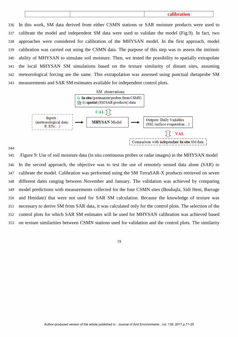
In this work, SM data derived from either CSMN stations or SAR moisture products were used to 336
calibrate the model and independent SM data were used to validate the model (Fig.9). In fact, two 337
approaches were considered for calibration of the MHYSAN model. In the first approach, model 338
calibration was carried out using the CSMN data. The purpose of this step was to assess the intrinsic 339
ability of MHYSAN to simulate soil moisture. Then, we tested the possibility to spatially extrapolate 340
the local MHYSAN SM simulations based on the texture similarity of distant sites, assuming 341
meteorological forcing are the same. This extrapolation was assessed using punctual thetaprobe SM 342
measurements and SAR SM estimates available for independent control plots. 343
344
Figure 9: Use of soil moisture data (in situ continuous probes or radar images) in the MHYSAN model 345
In the second approach, the objective was to test the use of remotely sensed data alone (SAR) to 346
calibrate the model. Calibration was performed using the SM TerraSAR-X products retrieved on seven 347
different dates ranging between November and January. The validation was achieved by comparing 348
model predictions with measurements collected for the four CSMN sites (Bouhajla, Sidi Heni, Barrage 349
and Hmidate) that were not used for SAR SM calculation. Because the knowledge of texture was 350
necessary to derive SM from SAR data, it was calculated only for the control plots. The selection of the 351
control plots for which SAR SM estimates will be used for MHYSAN calibration was achieved based 352
on texture similarities between CSMN stations used for validation and the control plots. The similarity 353
Author-produced version of the article published in : Journal of Arid Environments , vol. 139, 2017.p.11-25
20
was based on the the euclidean distances between texture components, namely percentage of clay, silt 354
and sand. 355
4 Results and Discussion 356
4.1 MHYSAN model calibration using SM measurements 357
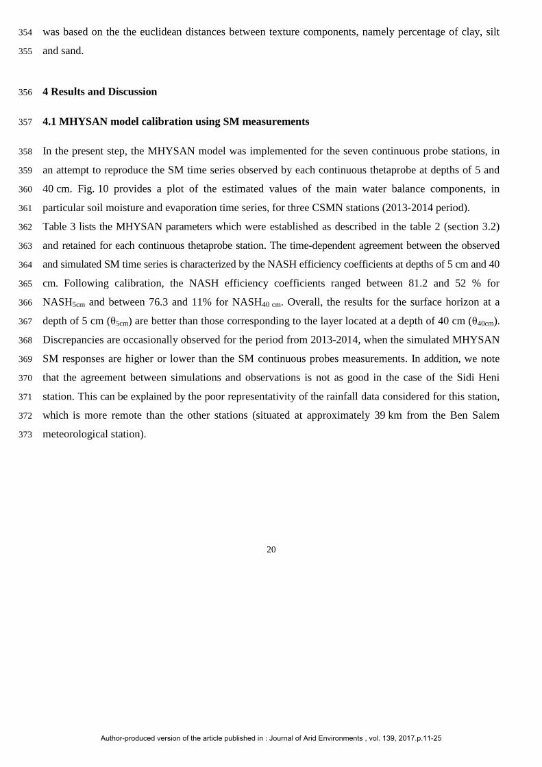
In the present step, the MHYSAN model was implemented for the seven continuous probe stations, in 358
an attempt to reproduce the SM time series observed by each continuous thetaprobe at depths of 5 and 359
40 cm. Fig. 10 provides a plot of the estimated values of the main water balance components, in 360
particular soil moisture and evaporation time series, for three CSMN stations (2013-2014 period). 361
Table 3 lists the MHYSAN parameters which were established as described in the table 2 (section 3.2) 362
and retained for each continuous thetaprobe station. The time-dependent agreement between the observed 363
and simulated SM time series is characterized by the NASH efficiency coefficients at depths of 5 cm and 40 364
cm. Following calibration, the NASH efficiency coefficients ranged between 81.2 and 52 % for 365
NASH5cm and between 76.3 and 11% for NASH40 cm. Overall, the results for the surface horizon at a 366
depth of 5 cm (θ5cm) are better than those corresponding to the layer located at a depth of 40 cm (θ40cm). 367
Discrepancies are occasionally observed for the period from 2013-2014, when the simulated MHYSAN 368
SM responses are higher or lower than the SM continuous probes measurements. In addition, we note 369
that the agreement between simulations and observations is not as good in the case of the Sidi Heni 370
station. This can be explained by the poor representativity of the rainfall data considered for this station, 371
which is more remote than the other stations (situated at approximately 39 km from the Ben Salem 372
meteorological station). 373
Author-produced version of the article published in : Journal of Arid Environments , vol. 139, 2017.p.11-25

21
(a) 374
(b) 375
(c) 376 Figure 10: Evaporation and soil moisture simulations using observed moisture measurements from (a) 377
Chebika (b) P12 (c) Barrage. “Obs θ5” and “Obs θ40” correspond to the SM time series observed using 378 continuous probes at depths of 5 cm and 40 cm respectively. “Sim θ5”and “Sim θ40” correspond to the 379
volumetric water content simulated by the MHYSAN model, at depths of 5 cm and 40 cm respectively. 380
Table 3. Soil Parameters retained after calibrating MHYSAN with measured values of moisture. 381
0
10
20
30
40
50
60
70
80
90
100
0
0.05
0.1
0.15
0.2
0.25
0.3
0.35
0.4
0.45
0.5
01/08/2013 01/10/2013 01/12/2013 01/02/2014 01/04/2014 01/06/2014 01/08/2014
Chebika station Rain
Obs_θ5
Obs_θ40
Sim_θ5
Sim_θ40
Evaporation
0
10
20
30
40
50
60
70
80
90
100
0
0.05
0.1
0.15
0.2
0.25
0.3
0.35
0.4
0.45
0.5
01/05/2013 16/06/2013 01/08/2013 16/09/2013 01/11/2013 17/12/2013 01/02/2014 19/03/2014 04/05/2014 19/06/2014 04/08/2014
P12 Station Rain
Obs_θ5
Obs_θ40
Sim_θ5
Sim_θ40
Evaporation
0
10
20
30
40
50
60
70
80
90
100
0
0.05
0.1
0.15
0.2
0.25
0.3
0.35
0.4
0.45
0.5
01/05/2013 16/06/2013 01/08/2013 16/09/2013 01/11/2013 17/12/2013 01/02/2014 19/03/2014 04/05/2014 19/06/2014 04/08/2014
Barrage station RainObs_θ5Obs_θ40Sim_θ5Sim_θ40Evaporation
Author-produced version of the article published in : Journal of Arid Environments , vol. 139, 2017.p.11-25

22
Ze (mm)
Zd (mm)
θfc 5cm [m3m-3]
θres5cm [m3m-3]
θfc 40cm [m3m-3]
θres40cm [m3m-3]
RE [mm]
cdif [mm.day-1]
NASH5cm
NASH40cm
Chebika station
194.5 500 0.37 0.04 0.27 0.1 -5.57 6.23 81.2 26.2
P12 station
188 866 0.24 0.03 0.2 0.09 -21.7 3.47 66 63.2
Hmidate station
225 500 0.1 0.03 0.11 0.06 -25.1 0.31 62.4 50.8
Barrage station
225 679 0.28 0.05 0.23 0.12 -15.1 5.98 68 49
Barrouta station
225 680 0.21 0.04 0.11 0.03 -1.13 3.36 63 76.3
Bouhajla station
225 280 0.16 0.01 0.11 0.01 -10 3.05 58 39.1
Sidi Heni station
225 318 0.27 0.07 0.14 0.1 -84.8 2.34 52 11
382
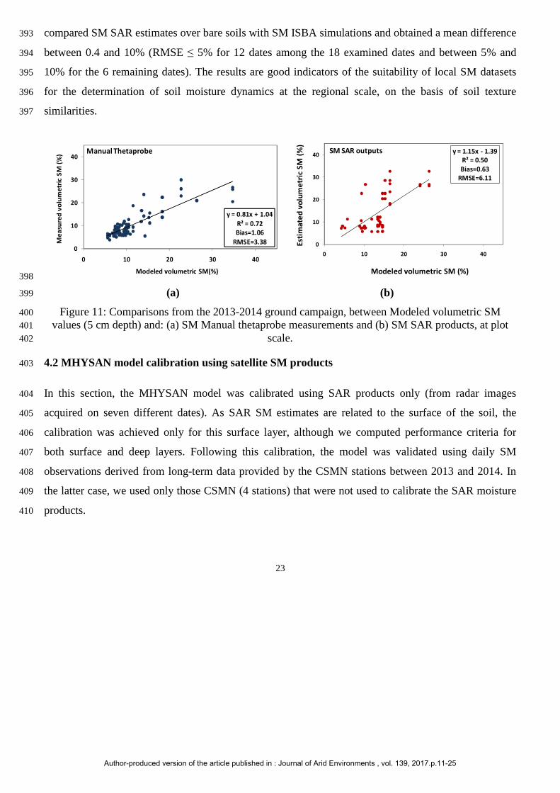
Then, we propose a comparison of calibrated MHYSAN SM outputs at plot scale with in situ SM data 383
and SAR moisture estimations. These comparisons take into account texture similarities, as well as the 384
location between continuous probe stations and control plots for 2013-2014 season (only stations close 385
to the control plots were used). In Fig. 11, we compare the MHYSAN surface SM at 5cm depth with 386
plot scale estimations made using: a) manual thetaprobe, and b) SAR moisture. In the last case, the 387
CSMN3 used to calibrate the SAR moisture products, were removed from these comparisons. At plot 388
scale, the results are characterized by a volumetric moisture bias and RMSE equal to 1.06 and 3.38% 389
respectively, when the MHYSAN SM simulations are compared to the SM manual thetaprobe 390
measurements. Similarly, the comparison between MHYSAN SM and SM SAR outputs leads to a 391
volumetric moisture bias and an RMSE equal to 0.63 and 6.11%, respectively. Baghdadi et al., 2007 392
Author-produced version of the article published in : Journal of Arid Environments , vol. 139, 2017.p.11-25
23
compared SM SAR estimates over bare soils with SM ISBA simulations and obtained a mean difference 393
between 0.4 and 10% (RMSE ≤ 5% for 12 dates among the 18 examined dates and between 5% and 394
10% for the 6 remaining dates). The results are good indicators of the suitability of local SM datasets 395
for the determination of soil moisture dynamics at the regional scale, on the basis of soil texture 396
similarities. 397
398
(a) (b) 399
Figure 11: Comparisons from the 2013-2014 ground campaign, between Modeled volumetric SM 400 values (5 cm depth) and: (a) SM Manual thetaprobe measurements and (b) SM SAR products, at plot 401
scale. 402
4.2 MHYSAN model calibration using satellite SM products 403
In this section, the MHYSAN model was calibrated using SAR products only (from radar images 404
acquired on seven different dates). As SAR SM estimates are related to the surface of the soil, the 405
calibration was achieved only for this surface layer, although we computed performance criteria for 406
both surface and deep layers. Following this calibration, the model was validated using daily SM 407
observations derived from long-term data provided by the CSMN stations between 2013 and 2014. In 408
the latter case, we used only those CSMN (4 stations) that were not used to calibrate the SAR moisture 409
products. 410
y = 0.81x + 1.04
R² = 0.72
Bias=1.06
RMSE=3.380
10
20
30
40
0 10 20 30 40
Me
asu
red
vo
lum
etr
ic S
M (
%)
Modeled volumetric SM(%)
Manual Thetaprobe y = 1.15x - 1.39
R² = 0.50
Bias=0.63
RMSE=6.11
0
10
20
30
40
0 10 20 30 40
Est
ima
ted
vo
lum
etr
ic S
M (
%)
Modeled volumetric SM (%)
SM SAR outputs
Author-produced version of the article published in : Journal of Arid Environments , vol. 139, 2017.p.11-25

24
As no SAR SM estimations were available for the areas corresponding to the four CSMN stations used 411
to validate MHYSAN, the SAR SM corresponding to control plots with textures similar to that of each 412
respective station were used. Four different control-plot groups were thus selected, on the basis of the 413
Euclidean distance between their texture and that of their respective stations. Only distances of less than 414
10 were retained. For each texture group, the relevant SAR SM value was computed as the mean of the 415
SM values determined for the corresponding control plots. 416
Fig. 12 shows the resulting estimated water balance variables, surface SM and evaporation, computed 417
by the MHYSAN model using seven SAR SM products for the four different plots corresponding to 418
each of the validation stations. The discrepancies between the estimated SM SAR products and the 419
simulated SM MHYSAN outputs are presented in Table 4, showing that globally satisfactory 420
simulations are achieved. The use of just seven SAR SM estimations leads to good model performance. 421
Brocca et al., 2008 reported the calibration of a conceptual model for soil water content balance, using a 422
small number of isolated SM measurements. In this study, variations in RMSE and NASH values were 423
determined as a function of the number of SM measurements (ranging from 3 to 15) used to calibrate 424
the model. The results revealed that just seven SM measurements were sufficient to obtain good RMSE 425
and NASH values, and to correctly calibrate the tested soil hydrological balance model. 426
We see on fig. 12 that although the seven satellite acquisition were achieved in a short time range as 427
compared to the simulation length, the SAR moisture values vary considerably over time, due to 428
important rainfall occurring during this period, which may have influenced positively our results. 429
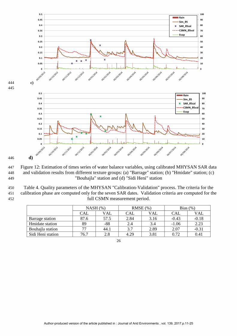
Fig. 12 plots the calibrated MHYSAN SM outputs, together with the continuous thetaprobe SM 430
observations. The Nash efficiency and statistical performance of these outputs are provided in Table 4. 431
The validated version of the calibrated MHYSAN model is generally found to be in good agreement 432
with the continuous probe observations and the MHYSAN simulations (Fig. 12 and Table 4). The 433
performances shown in this table also indicate that there is a poor agreement between the simulations and 434
observations in the case of the Sidi Heni and Hmidate stations. For the Sidi Heni station, this outcome 435
can be explained mainly by the poorly representative rainfall data used for this station. Indeed, an 436
Author-produced version of the article published in : Journal of Arid Environments , vol. 139, 2017.p.11-25
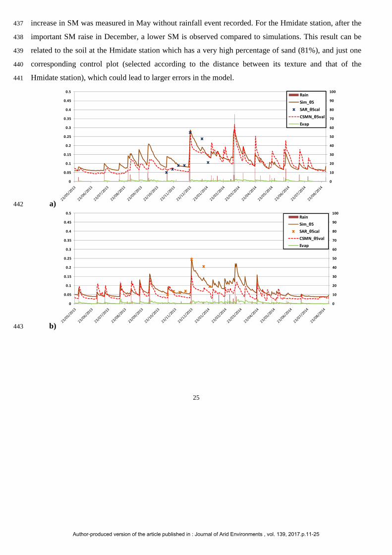
25
increase in SM was measured in May without rainfall event recorded. For the Hmidate station, after the 437
important SM raise in December, a lower SM is observed compared to simulations. This result can be 438
related to the soil at the Hmidate station which has a very high percentage of sand (81%), and just one 439
corresponding control plot (selected according to the distance between its texture and that of the 440
Hmidate station), which could lead to larger errors in the model. 441
a) 442
b) 443
0
10
20
30
40
50
60
70
80
90
100
0
0.05
0.1
0.15
0.2
0.25
0.3
0.35
0.4
0.45
0.5Rain
Sim_θ5
SAR_θ5cal
CSMN_θ5val
Evap
0
10
20
30
40
50
60
70
80
90
100
0
0.05
0.1
0.15
0.2
0.25
0.3
0.35
0.4
0.45
0.5Rain
Sim_θ5
SAR_θ5cal
CSMN_θ5val
Evap
Author-produced version of the article published in : Journal of Arid Environments , vol. 139, 2017.p.11-25
26
c) 444 445
d) 446
Figure 12: Estimation of times series of water balance variables, using calibrated MHYSAN SAR data 447 and validation results from different texture groups: (a) "Barrage" station; (b) "Hmidate" station; (c) 448
"Bouhajla" station and (d) "Sidi Heni" station 449
Table 4. Quality parameters of the MHYSAN "Calibration-Validation" process. The criteria for the 450 calibration phase are computed only for the seven SAR dates. Validation criteria are computed for the 451
full CSMN measurement period. 452
NASH (%) RMSE (%) Bias (%) CAL VAL CAL VAL CAL VAL
Barrage station 87.6 57.5 2.84 3.16 -0.43 -0.18 Hmidate station 89 -88 2.4 3.4 -1.06 2.23 Bouhajla station 77 44.1 3.7 2.89 2.07 -0.31 Sidi Heni station 76.7 2.8 4.29 3.81 0.72 0.41
0
10
20
30
40
50
60
70
80
90
100
0
0.05
0.1
0.15
0.2
0.25
0.3
0.35
0.4
0.45
0.5
Rain
Sim_θ5
SAR_θ5cal
CSMN_θ5val
Evap
0
10
20
30
40
50
60
70
80
90
100
0
0.05
0.1
0.15
0.2
0.25
0.3
0.35
0.4
0.45
0.5Rain
Sim_θ5
SAR_θ5cal
CSMN_θ5val
Evap
Author-produced version of the article published in : Journal of Arid Environments , vol. 139, 2017.p.11-25
27
Finally, the MHYSAN simulations using SAR SM products for calibration were compared with 453
MHYSAN outputs obtained using bibliographic FAO parameters only. The Ze and Zsol depth were 454
fixed respectively at 100 and 700 mm in order to fit with the SM probe depth. The soil resistance to 455
evaporation RE was determined using the REW values proposed by FAO for various soils textures 456
(table 19 of the FAO 56 paper), as well as the soil moisture values θres and θfc. Finally, the diffusion 457
coefficient was arbitrary fixed to the medium value of 2 as observed for several calibrations achieved in 458
previous studies (not shown here). The Nash efficiency and statistical performance of these simulations 459
are listed in Table 5, showing that the MHYSAN model performs better when SAR SM products are 460
used. These results confirm the effectiveness of TerraSAR-X SM retrieval for the calibration of a bare 461
soil hydrological model. 462
Table 5. Quality parameters of the MHYSAN model using FAO parameters only 463
NASH (%) RMSE (%) Bias (%) Barrage station -151 12.84 9.96 Hmidate station -259 13.69 11.63 Bouhajla station 70.2 4.22 1.42 Sidi Heni station -423 20.36 18.31
5 Conclusions 464
This study was designed to investigate the potential of high-resolution TerraSAR-X soil moisture (SM) 465
products for the calibration of a soil water balance model. We used MHYSAN, a bare soil hydrological 466
balance model, which simulates soil evaporation and moisture content over bare soil using as 467
input meteorological data. The model was first calibrated using time series of daily SM continuously 468
measured for some sites. The results had good NASH efficiencies ranged between 81.2 and 52 % for 469
NASH5cm and between 76.3 and 11% for NASH40 cm, thus showing that the MHYSAN model is able to 470
correctly reproduce the SM. Validation of calibrated output SM was based on comparison over control 471
plots with manual thetaprobe measurements and SM products obtained by SAR image processing. 472
These comparisons were made on the basis of texture similarities between continuous probes and 473
control plots. The results have a bias of approximately 1.06 and 0.63, and an RMSE equal to 3.38% and 474
Author-produced version of the article published in : Journal of Arid Environments , vol. 139, 2017.p.11-25
28
6.11%, for the ground volumetric SM determined using manual thetaprobe and SAR moisture maps, 475
respectively. 476
The model was then calibrated using SAR SM maps retrieved on seven different dates ranging over two 477
months and was then validated using moisture data recorded at continuous probe stations during 15 478
months. We show that the model performs well with NASH efficiencies ranged between 76.7 and 89%, 479
thus demonstrating that SAR data can actually be used to calibrate SM models without requiring 480
ground data. High agreement is observed between calibrated model and continuous thetaprobe 481
measurements. These results show that a simple SM model combined this SAR images acquired 482
for contrasted moisture condition may allow estimates of daily SM. An optimal use of this 483
approach could be achieved by using moisture data collected at different times of the year, during the 484
rainy season and the dry season, since the model's performance will necessarily vary for different types 485
of case study. The study presented here should be extended to other areas, in particular those 486
presenting other soil types (covered soils, degraded soils …). Moreover, progress in the 487
parameterization of this model could benefit from a more varied range of SAR data. 488
The main limitation relies in the representatively of the meteorological forcing used. Indeed, if 489
rainfall data is not reliable, a frequent configuration in semi arid areas, then the model although 490
locally well calibrated will not be able to work correctly. In this case the solution would be to use 491
remote sensing not only to calibrate the model, but to monitor rainfall and the SM themselves. 492
This opportunity is about to be offered in the coming month thanks to the Sentinel-1 mission 493
which represent a considerable breakthrough providing frequent and free high resolution SAR 494
data all over the world. In future research, we plan to optimize and apply this approach to the case of 495
Sentinel1 SAR data, allowing moisture estimations to be made at a higher repeat rate, over longer 496
periods of time. 497
Author Contributions 498
Azza Gorrab and Vincent Simonneaux: data processing; data analysis and interpretation of results. 499
Author-produced version of the article published in : Journal of Arid Environments , vol. 139, 2017.p.11-25
29
Mehrez Zribi: SAR data analysis and interpretation of results. 500 Sameh Saadi: data processing. 501 Nicolas Baghdadi: SAR data analysis. 502 Zohra Lili-Chabaane: organization of experimental campaigns. 503 Pascal Fanise: site instrumentation. 504
Acknowledgments 505
This study was funded by the MISTRALS/SICMED, ANR AMETHYST (ANR-12 TMED-0006-01) and 506
TOSCA/CNES projects. We wish to thank all of the technical teams from the IRD and INAT (Institut National 507
Agronomique de Tunisie) for their consistent collaboration and support during the implementation of ground-508
truth measurements. We are grateful for the financial support provided by the ANR/TRANSMED program for 509
the AMETHYST project (ANR-12-TMED-0006-01), as well as the mobility support provided by the PHC 510
Maghreb program (N° 32592VE). The authors wish to thank the German Space Agency (DLR) for kindly 511
providing them with TSX images under proposal HYD0007. 512
References 513
Albergel, C., Zakharova, E., Calvet, J. C., Zribi, M., Pardé, M., Wigneron, J. P., Novello, N., Kerr, Y., Mialon, 514 A., NouredDine Fritz. A first assessment of the SMOS data in southwestern France using in situ and airborne soil 515 moisture estimates: the CAROLS airborne campaign, Remote Sensing of Environment, 115, 2718–2728, 2011. 516
Allen, R.G.; Pereira, L.S.; Raes, D.; Smith, M. Crop Evapotranspiration—Guidelines for Computing Crop Water 517 Requirements; FAO Irrigation and Drainage Paper 56; FAO: Rome, Italy, p. 300, 1998. 518
Amri, R., Zribi, M., Chabaane, Z. L., Wagner, W., & Hasenauer, S. Analysis of C-band scatterometer moisture 519 estimations derived over a semiarid region. Geoscience and Remote Sensing, IEEE Transactions on Geoscience 520 and Remote Sensing. 50(7), 2630-2638, 2012. 521
Aubert D., Loumagne C., Oudin L. et Le Hégarat-Mascle S., 2003. Assimilation of soil moisture into 522 hydrological models: the sequential method. Canadian journal of remote sensing, 29(6), 711-717. 523
Baghdadi N., Aubert M., Cerdan O., Franchistéguy L., Viel C., Martin E., Zribi M., Desprats J.F. Operational 524 mapping of soil moisture using synthetic aperture radar data: application to the Touch Basin (France). Sensors 525 Journal, vol. 7: 2458-2483, 2007. 526
Author-produced version of the article published in : Journal of Arid Environments , vol. 139, 2017.p.11-25

30
Baghdadi, N.; Cerdan, O.; Zribi, M.; Auzet, V.; Darboux, F.; Hajj, M.E.; Kheir, R.B. Operational performance of 527 current synthetic aperture radar sensors in mapping soil surface characteristics in agricultural environments: 528 Application to hydrological and erosion modelling. Hydrol. Proc. 22, 9–20, 2008. 529
Barrett, B.W.; Dwyer, E.; Padraig, W. Soil moisture retrieval from active space born microwave observations: An 530 evaluation of current techniques. Remote Sens. 1, 210–242, 2009. 531
Bezerra, B.G.; dos Santos, C.A.C.; da Silva, B.B.; Perez-Marin, A.M.; Bezerra, M.V.C.; Bezerra, J.R.C.; Ramana 532 Rao, T.V. Estimation of soil moisture in the root-zone from remote sensing data. Rev. Bras. Ciênc. Solo. 37, 533 596–603, 2013. 534
Brocca L, Melone F, Moramarco T. Empirical and conceptual approaches for soil moisture estimation in view of 535 event-based rainfall–runoff modeling. In Progress in Surface and Subsurface Water Studies at the Plot and Small 536 Basin Scale, Maraga F, Arattano M (eds). IHP-VI, Technical Documents in Hydrology No. 77. UNESCO: Paris; 537 1–8, 2005. 538
Brocca L., Melone F., Moramarco T., Wagner W., Naeimi V., Bartalis Z., Hasenauer S. Improving runoff 539 prediction through the assimilation of the ASCAT soil moisture product. Hydrology and Earth System Sciences, 540 14(10):1881–1893, 2010. 541
Brocca, L., Melone, F., & Moramarco, T. On the estimation of antecedent wetness conditions in rainfall–runoff 542 modelling. Hydrological Processes, 22(5), 629-642, 2008. 543
Brocca, L., Moramarco, T., Melone, F., Wagner, W., Hasenauer, S., and Hahn, S.: Assimilation of surface and 544 root-zone ASCAT soil moisture products into rainfall-runoff modelling,. IEEE T. Geosci. Remote, 50, 2542–545 2555, 2012. 546
Chen, X. and Hu, Q. Groundwater influences on soil moisture and surface evaporation. Journal of Hydrology, 547 297(1), 285-300, 2004. 548
Doubková, M.; van Dijk, A.I.J.M.; Sabel, D.; Wagner, W.; Blöschl, G. Evaluation of the predicted error of the 549 soil moisture retrieval from C-band SAR by comparison against modeled soil moisture estimates over Australia. 550 Remote Sens. Environ. 2012, 120(2), 188–196. doi: 10.1016/j.rse.2011.09.031 551
Draper, C., Mahfouf, J.-F., Calvet, J.-C., Martin, E., and Wagner, W., 2011. Assimilation of ASCAT near-surface 552 soil moisture into the SIM hydrological model over France, Hydrol. Earth Syst. Sci., 15, 3829–3841, 553 doi:10.5194/hess-15-3829-2011. 554
Entekhabi D, Rodriguez-lturbe I. 1994. An analytic framework for the characterization of the space–time 555 variability of soil moisture. Advances in Water Resources 17: 25–45. 556
Er-Raki, S.; Chehbouni, A.; Guemouria, N.; Duchemin, B.; Ezzahar, J.; Hadria, R. Combining fao-56 model and 557 ground-based remote sensing to estimate water consumptions of wheat crops in a semi-arid region. Agric. Water 558 Manag. 87, 41–54, 2007. 559
Author-produced version of the article published in : Journal of Arid Environments , vol. 139, 2017.p.11-25
31
Famiglietti, J. S., & Wood, E. F. (1994). Multiscale modeling of spatially variable water and energy balance 560 processes. Water Resources Research, 30(11), 3061-3078. DOI: 10.1029/94WR01498 561
Famiglietti, J. S., Rudnicki, J. W., & Rodell, M. (1998). Variability in surface moisture content along a hillslope 562 transect: Rattlesnake Hill, Texas. Journal of Hydrology, 210(1), 259-281. http://dx.doi.org/10.1016/S0022-563 1694(98)00187-5 564
François, C., Quesney, A., and Ottle, C.: Sequential assimilation of ERS-1 SAR data into a coupled land surface-565 hydrological model using an extended Kalman filter, Hydrometeorol., 4, 473–487, 2003. 566
Gorrab, A.; Zribi, M.; Baghdadi, N.; Mougenot, B.; Fanise, P.; Lili Chabaane, Z. Retrieval of Both Soil Moisture 567 and Texture Using TerraSAR-X Images. Remote Sens., 7, 10098-10116, 2015b. 568
Gorrab, A.; Zribi, M.; Baghdadi, N.; Mougenot, B.; Lili Chabaane, Z. Potential of X-Band TerraSAR-X and 569 COSMO-SkyMed SAR Data for the assessment of physical soil parameters. Remote Sens. 7, 747–766, 2015a. 570
Gowda, P.; Chavez, J.; Colaizzi, P.; Evett, S.; Howell, T.; Tolk, J. ET mapping for agricultural water 571 management: Present status and challenges. Irrig. Sci., 26, 223–237, 2008. 572
Iacobellis, V., Gioia, A., Milella, P., Satalino, G., Balenzano, A., & Mattia, F. (2013). Inter-comparison of 573 hydrological model simulations with time series of SAR-derived soil moisture maps. European Journal of 574 Remote Sensing, 46(1), 739-757. 575
Koster, R.D.; Dirmeyer, P.A.; Guo, Z.; Bonan, G.; Chan, E.; Cox, P.; Gordon, C.T.; Kanae, S.; Kowalczyk, E.; 576 Lawrence, D.; et al. Regions of strong coupling between soil moisture and precipitation. Science, 305, 1138–577 1140, 2004. 578
Li, Z.L.; Tang, R.L.; Wan, Z.M.; Bi, Y.Y.; Zhou, C.H.; Tang, B.H.; Yan, G.J.; Zhang, X.Y. A review of current 579 methodologies for regional evapotranspiration estimation from remotely sensed data. Sensors, 9, 3801–3853, 580 2009. 581
Lievens, H., Tomer, S. K., Al Bitar, A., De Lannoy, G. J. M., Drusch, M., Dumedah, G., Hendricks Franssen, H.-582 J., Kerr, Y. H., Martens, B., Pan, M., Roundy, J. K., Vereecken, H.,Walker, J. P., Wood, E. F., Verhoest, N. E. C. 583 and Pauwels, V. R. N., 2015. SMOS soil moisture assimilation for improved hydrologic simulation in the Murray 584 Darling Basin, Australia, Remote Sens. Environ., 168, 146–162. 585
López López, P., Wanders, N., Schellekens, J., Renzullo, L. J., Sutanudjaja, E. H., and Bierkens, M. F. P. (2016). 586 Improved large-scale hydrological modelling through the assimilation of streamflow and downscaled satellite soil 587 moisture observations. Hydrol. Earth Syst. Sci., 20(7), 3059-3076, doi: 10.5194/hess-20-3059-2016. 588
Manfreda S., Fiorentino M., Iacobellis V. (2005) - DREAM: a distributed model for runoff, evapotranspiration, 589 and antecedent soil moisture simulation. Advanced Geosciences, 2: 31-39. doi: http://dx.doi.org/10.5194/adgeo-590 2-31-2005. 591
Author-produced version of the article published in : Journal of Arid Environments , vol. 139, 2017.p.11-25
32
Massari, C.; Brocca, L.; Tarpanelli, A.; Moramarco, T., 2015.Data Assimilation of Satellite Soil Moisture into 592 Rainfall-Runoff Modelling: A Complex Recipe? Remote Sens. 2015, 7, 11403-11433. 593
Matgen, P., Henry, J. B., Hoffmann, L. and Pfister, L., 2006. Assimilation of remotely sensed soil saturation 594 levels in conceptual rainfall-runoff models. IAHS-AISH publication, 226-234. 595
Pandey, V.; Pandey, P.K. Spatial and temporal variability of soil moisture. Int. J. Geosci., 1, 87-98, 2010. 596
Pathe, C.; Wagner, W.; Sabel, D.; Doubkova, M.; Basara, J.B. Using ENVISAT ASAR global mode data for 597 surface soil moisture retrieval over Oklahoma, USA. IEEE Trans. Geosci. Remote Sens., 47, 468–480, 2009. 598
Pauwels, V. R. N., Hoeben, R., Verhoest, N. E. C., De Troch, F. P. and Troch, P. A. (2002), Improvement of 599 TOPLATS-based discharge predictions through assimilation of ERS-based remotely sensed soil moisture values. 600 Hydrol. Process., 16: 995–1013. doi:10.1002/hyp.315 601
Pierdicca, N., Pulvirenti, L., Brocca, L., & Fascetti, F. (2014). Multitemporal Soil Moisture Retrieval from Three-602 Day Repeat ERS/SAR Data. Proceedings EUSAR 2014; 10th International European Conference on Synthetic 603 Aperture Radar; Berlin, 3-5 June 2014. 604
Qin, J., Liang, S., Yang, K., Kaihotsu, I., Liu, R. and Koike, T., 2009. Simultaneous estimation of both soil 605 moisture and model parameters using particle filtering method through the assimilation of microwave signal. 606 Journal of Geophysical Research: Atmospheres, 114(D15) 607
Renzullo, L. J., van Dijk, A. I. J. M., Perraud, J. M., Collins, D., Henderson, B., Jin, H., and McJannet, D. L.: 608 Continental satellite soil moisture data assimilation improves root-zone moisture analysis for water resources 609 assessment, J. Hydrol., 519, 2747– 2762, 2014. 610
Saadi, S.; Simonneaux, V.; Boulet, G.; Raimbault, B.; Mougenot, B.; Fanise, P.; Ayari, H.; Lili-Chabaane, Z. 611 Monitoring Irrigation Consumption Using High Resolution NDVI Image Time Series: Calibration and Validation 612 in the Kairouan Plain (Tunisia). Remote Sens. 7, 13005–13028, 2015. 613
Santi, E., Paloscia, S., Pettinato, S., Notarnicola, C., Pasolli, L., & Pistocchi, A. (2013). Comparison between 614 SAR soil moisture estimates and hydrological model simulations over the Scrivia test site. Remote Sensing, 5(10), 615 4961-4976. 616
Seneviratne, S.I.; Corti, T.; Davin, E.L.; Hirschi, M.; Jaeger, E.B.; Lehner, I.; Orlowsky, B.; Teuling, A.J. 617 Investigating soil moisture-climate interactions in a changing climate: A review. Earth-Sci. Rev., 99, 125–161, 618 2010. 619
Shabou, M; Mougenot, B.; Lili Chabaane, Z.; Walter, C.; Boulet, G.; Ben Aissa, N.; Zribi, M. 620 Soil clay content mapping using a time series of Landsat TM data in semi-arid lands. 621 Remote Sens., 7, 6059–6078, 2015. 622
Author-produced version of the article published in : Journal of Arid Environments , vol. 139, 2017.p.11-25
33
Simonneaux, V.; Duchemin, B.; Helson, D.; ErRaki, S.; Olioso, A.; Chehbouni, A. The use of high resolution 623 image time series for crop classification and evapotranspiration estimate over an irrigated area in central 624 morocco. Int. J. Remote Sens., 29, 95–116, 2008. 625
Simonneaux, V.; Lepage, M.; Helson, D.; Métral, J.; Thomas, S.; Duchemin, B.; Cherkaoui, M.; Kharrou, H.; 626 Berjami, B., and Chebhouni, A. Estimation spatialisée de l'évapotranspiration des cultures irriguées par 627 télédétection: Application à la gestion de l'irrigation dans la plaine du haouz (Marrakech, Morocco). Sécheresse, 628 20, 123-130, 2009. 629
Sutanto, S. J., Wenninger, J., Coenders-Gerrits, A. M. J., and Uhlenbrook, S.: Partitioning of evaporation into 630 transpiration, soil evaporation and interception: a comparison between isotope measurements and a HYDRUS-1D 631 model, Hydrol. Earth Syst. Sci., 16, 2605-2616, doi:10.5194/hess-16-2605-2012, 2012. 632
Tramblay, Y., Bouaicha, R., Brocca, L., Dorigo, W., Bouvier, C., Camici, S., & Servat, E. Estimation of 633 antecedent wetness conditions for flood modelling in northern Morocco. Hydrology and Earth System Sciences, 634 16(11), 4375-4386, 2012. 635
Wagner, W.; Pathe, C.; Doubkova, M.; Sabel, D.; Bartsch, A.; Hasenauer, S.; Blöschl, G.; Scipal, K.; Martínez-636 Fernández, J.; Löw, A. Temporal stability of soil moisture and radar backscatter observed by the Advanced 637 Synthetic Aperture Radar (ASAR). Sensors, 8, 1174–1197, 2008. 638
Weisse A., Oudin L. et Loumagne C. Assimilation of soil moisture into hydrological models for flood 639 forecasting: comparison of a conceptual rainfall-runoff model and a model with an explicit counterpart for soil 640 moisture. Revue des sciences de l’Eau, Rev.Sci.Eau. 16/2, 173-197, 2003. 641
Zehe E, Bloschl G. Predictability of hydrologic response at the plot and catchment scales: role of initial 642 condition. Water Resources Research 40: W10202. 2004. 643
Zhang, X., Zhang, X., Li, G. The effect of texture and irrigation on the soil moisture vertical-temporal variability 644 in an urban artificial landscape: A case study of Olympic Forest Park in Beijing. Front. Environ. Sci. Eng., 9, 645 269–278, 2015. 646
Zribi, M.; Chahbi, A.; Shabou, M.; Lili-Chabaane, Z.; Duchemin, B.; Baghdadi, N.; Amri, R.; Chehbouni, A. Soil 647 surface moisture estimation over a semi-arid region using Envisat ASAR radar data for soil evaporation 648 evaluation. Hydrol. Earth Syst. Sci. 15, 345–358, 2011. 649
Zribi, M., Baghdadi, N., Holah, N., Fafin, O., and Guérin, C. Evaluation of a rough soil surface description with 650 ASAR-ENVISAT Radar Data, Remote sensing of environment, Vol. 95, 67-76, 2005. 651
Author-produced version of the article published in : Journal of Arid Environments , vol. 139, 2017.p.11-25
Recommended