Diagnostic calibration of a hydrological model in an … 11, 1253–1300, 2014 Diagnostic calibration of a hydrological model in an alpine area Z. He et al. Title Page Abstract Introduction

HESSD11, 1253–1300, 2014

Diagnosticcalibration of a

hydrological model inan alpine area

Z. He et al.

Title Page

Abstract Introduction

Conclusions References

Tables Figures

J I

J I

Back Close

Full Screen / Esc

Printer-friendly Version

Interactive Discussion

Discussion

Paper

|D

iscussionP

aper|

Discussion

Paper

|D

iscussionP

aper|

Hydrol. Earth Syst. Sci. Discuss., 11, 1253–1300, 2014www.hydrol-earth-syst-sci-discuss.net/11/1253/2014/doi:10.5194/hessd-11-1253-2014© Author(s) 2014. CC Attribution 3.0 License.

Hydrology and Earth System

Sciences

Open A

ccess

Discussions

This discussion paper is/has been under review for the journal Hydrology and Earth SystemSciences (HESS). Please refer to the corresponding final paper in HESS if available.

Diagnostic calibration of a hydrologicalmodel in an alpine areaZ. He1, F. Tian1, H. C. Hu1, H. V. Gupta2, and H. P. Hu1

1State Key Laboratory of Hydroscience and Engineering, Department of HydraulicEngineering, Tsinghua University, Beijing, 100084, China2Department of Hydrology and Water Resources, The University of Arizona,Tucson, Arizona, 85721, USA

Received: 19 November 2013 – Accepted: 10 January 2014 – Published: 23 January 2014

Correspondence to: F. Tian ([email protected])

Published by Copernicus Publications on behalf of the European Geosciences Union.

1253

http://www.hydrol-earth-syst-sci-discuss.net

http://www.hydrol-earth-syst-sci-discuss.net/11/1253/2014/hessd-11-1253-2014-print.pdf

http://www.hydrol-earth-syst-sci-discuss.net/11/1253/2014/hessd-11-1253-2014-discussion.html

http://creativecommons.org/licenses/by/3.0/

HESSD11, 1253–1300, 2014



Z. He et al.

Title Page



Tables Figures

J I

J I

Back Close

Full Screen / Esc



Discussion

Paper

|D

iscussionP

aper|

Discussion

Paper

|D

iscussionP

aper|

Abstract

Hydrological modeling depends on single- or multiple-objective strategies for param-eter calibration using long time sequences of observed streamflow. Here, we demon-strate a diagnostic approach to the calibration of a hydrological model of an alpinearea in which we partition the hydrograph based on the dominant runoff generation5

mechanism (groundwater baseflow, glacier melt, snowmelt, and direct runoff). The par-titioning reflects the spatiotemporal variability in snowpack, glaciers, and temperature.Model parameters are grouped by runoff generation mechanism, and each group iscalibrated separately via a stepwise approach. This strategy helps to reduce the prob-lem of equifinality and, hence, model uncertainty. We demonstrate the method for the10

Tailan River basin (1324 km2) in the Tianshan Mountains of China with the help of asemi-distributed hydrological model (THREW).

1 Introduction

1.1 Background

Parameter calibration has been singled out as one of the major issues in the applica-15

tion of hydrological models (Johnston and Pilgrim, 1976; Gupta and Sorooshian, 1983;Beven and Binley, 1992; Boyle et al., 2000). Commonly, one or more objective func-tions are selected as criteria to evaluate the similarity between observed and simulatedhydrographs (Nash and Sutcliffe, 1970; Brazil, 1989; Gupta et al., 1998; van Griensvenand Bauwens, 2003). As model complexity increases, parameter dimensionality also20

increases significantly. For this reason, automatic calibration procedures have beendeveloped to identify the optimal parameter set (Gupta and Sorooshian, 1985; Ganand Biftu, 1996; Vrugt et al., 2003a, b). However, given the limited capability of processunderstanding and measurement technologies, models have been developed that in-clude different parameter sets within a chosen space that may acceptably reproduce25

1254





HESSD11, 1253–1300, 2014



Z. He et al.

Title Page



Tables Figures

J I

J I

Back Close

Full Screen / Esc



Discussion

Paper

|D

iscussionP

aper|

Discussion

Paper

|D

iscussionP

aper|

the observed aspects of the catchment system (Sorooshian and Gupta, 1983; Bevenand Freer, 2001). This phenomenon has been called “equifinality”, and it causes un-certainty in simulation and prediction (Duan et al., 1992; Beven, 1993, 1996). The“equifinality” issue in hydrology calls for methods that are powerful enough to evalu-ate and correct models and therefore must be “diagnostic”, i.e. capable of pointing to5

what degree a realistic representation of the real world has been achieved and how themodel should be improved (Spear and Hornberger, 1980; Gupta et al., 1998, 2008).

However, traditional regression-based model evaluation strategies (e.g. based onthe use of Mean Squared Error or Nash Sutcliffe Efficiency as performance criteria)are demonstrably poor in their ability to identify the roles of various model components10

or parameters in the model output (Van Straten and Keesman, 1991), which is duein part to the loss of meaningful information when projecting from the high dimensionof the data set down to the low (often one) dimension of the measure (Yilmaz et al.,2008; Gupta et al., 2009). A diagnostic evaluation method should match the numberof unknowns (parameters) with the number of pieces of information by making use15

of multiple measures of model performance (Gupta et al., 1998, 2008, 2009; Yilmazet al., 2008). One way to exploit hydrological information is to analyze the spatiotempo-ral characteristics of hydrological variables that can be related to specific hydrologicalprocesses in the form of “signature indices” (Richter et al., 1996; Sivapalan et al., 2003;Yilmaz et al., 2008). Ideally, a “signature” should represent some “invariant” property20

of the system, be readily identifiable from available data, directly reflect some systemfunction, and be maximally related to some “structure” or “parameter” in the model.

Attention to hydrological signatures, therefore, constitutes the natural basis for modeldiagnosis (Gupta et al., 2008). Placed in this context, the body of literature on the topicis indeed large. Yadav et al. (2007) used similarity indices and hydrological signatures25

(runoff ratio and slope of the flow duration curve – FDC) to classify catchments. Shamiret al. (2005a) described a parameter estimation method based on hydrograph descrip-tors (total flow, range between the extreme values, monthly rising limb density of thehydrograph, monthly maximum flow and negative/positive change) that characterize

1255





HESSD11, 1253–1300, 2014



Z. He et al.

Title Page



Tables Figures

J I

J I

Back Close

Full Screen / Esc



Discussion

Paper

|D

iscussionP

aper|

Discussion

Paper

|D

iscussionP

aper|

dominant streamflow patterns at three time scales (monthly, yearly, and record extent).Detenbeck et al. (2005) calculated several hydrologic indices including daily flow in-dices (mean, median, coefficient of variation and skewness), overall flood indices (floodfrequency, magnitude, duration, and flood timing of various levels), low flow variables(mean annual daily minimum), and ranges of flow percentiles to study the relationship5

of the streamflow regime to watershed characteristics. Shamir et al. (2005b) presentedtwo streamflow indices to describe the shape of the hydrograph (rising/declining limbdensity, i.e. RLD and DLD) for parameter estimation in 19 basins. Farmer et al. (2003)evaluated the climate, soil and vegetation controls on the variability of water balancethrough the following four signatures: gradient of the annual yield frequency graph, av-10

erage yield over many years for each month, FDC and magnitude and shape of thehydrograph. Jothityangkoon et al. (2001) proposed a downward approach to evaluatethe model’s performance against appropriate signatures at progressively refined timescale. Signatures that governed the evaluation of model complexity were the inter-annual variability, mean monthly variation in runoff (called regime curve), and the FDC.15

Generally, the reported signatures have the following two characteristics: (1) theyconcentrate on the extraction of the hydrologically meaningful information containedin the hydrograph, and (2) they focus on either the entire study period or a specialcontinuous section of the entire period. However, they have occasionally consideredthe temporal variability of the runoff components and the dominance of different runoff20

generation mechanisms during different periods (Boyle et al., 2000). Arguably, the sig-natures in common use today insufficiently exploit the hydrograph information in thetime dimension or in relation to the dominant runoff generation mechanisms.

For the alpine areas, on one hand, the hydrological processes are usually more com-plex with snow/glacier melting and possibly soil freezing/thawing than those in warmer25

areas, which implies a larger dimension of parameter (RP) in the corresponding hydro-logical models. On the other hand, measured data set useful for model identificationis usually limited due to the sparse gauged network, which produces a small mea-surement dimension (RM) far lower than RP. This intensifies the issue of equifinality in

1256





HESSD11, 1253–1300, 2014



Z. He et al.

Title Page



Tables Figures

J I

J I

Back Close

Full Screen / Esc



Discussion

Paper

|D

iscussionP

aper|

Discussion

Paper

|D

iscussionP

aper|

parameter identification. To address this problem, related studies are putting efforts intotwo directions: the first one is to reduce the calibrated RP by estimating part parame-ters based on basin characteristics a priori. For example, Gurtz et al. (1999) proposeda parameterization method based on elevation, slop and shading derived from basinterrain. Gomez-Landesa and Rango (2002) obtained model parameters of ungauged5

basins from gauged basins by basin size, proximity of location and shape similarities;Eder et al. (2005) estimated most of the parameters a priori from basin physiographybefore an automatic calibration is applied. The parameterization method may involvesome uncertainties but be useful for the determination of insensitive parameters. Thesecond direction is expanding the RM by exploiting information from available data.10

For instance, Dunn and Colohan (1999) used baseflow data as an additional criteriafor model evaluation. Mendoza et al. (2003) exploited recession-flow data to estimatehydraulic parameters. Stahl et al. (2008) used glacier mass balance information com-bined with stream hydrographs to constrain the melt factors, and used the volume-areascaling approach to estimate changes in glacier area. The results indicate that glacier15

mass balance can reduce uncertainty both in parameter calibration and predictions.Konz and Seibert (2010) combined glacier mass balance data with discharge to findthe appropriate parameter sets generated by Monte Carlo analyses. Schaefli and Huss(2011) integrated seasonal point glacier mass balance information for model calibrationby modifying the GSM-SOCONT model. They used the winter accumulation and annual20

balance to determine the snow accumulation correction factor, snow melt factor andtemperature lapse rate. Enough seasonal glacier information is a pre-requisite for thismethod. Jost et al. (2012) introduced glacier volume loss calculated by digital elevationmodels to calibrate hydrologic model. Uncertainty analyses by a generalized likelihooduncertainty estimation (GLUE) procedure demonstrated that glacier volume is helpful25

to reduce parameter uncertainty even in catchments where lack mass balance data.Knowledge acquired from these researches is that using additional information (base-flow and glacier mass) can reduce parameter uncertainty effectively, which expand theRM significantly.

1257





HESSD11, 1253–1300, 2014



Z. He et al.

Title Page



Tables Figures

J I

J I

Back Close

Full Screen / Esc



Discussion

Paper

|D

iscussionP

aper|

Discussion

Paper

|D

iscussionP

aper|

Hydrograph separation could be another way to expand RM. Studies have confirmedthat a hydrograph can be dominated by various components in different response peri-ods (Haberlandt et al., 2001; Eder et al., 2005). Information about the dominant hydro-logical processes contained in a hydrograph can be extracted by hydrograph separationor partitioning; this has long been a topic of interest in the science of hydrology. Sev-5

eral methods have been proposed (Pinder and Jones, 1969; McCuen, 1989; Nathan,1990; Vivoni et al., 2007). In general, these can be divided into graphical methods,analytical methods, empirical methods, geochemical methods and automated programtechniques (Nejadhashemi et al., 2009). Most of them primarily focus on the partition-ing of baseflow and are not capable of identifying more than two components. With10

the advance of isotope methods, multi-component hydrograph separation models havebeen developed. However, these models should be run on an extended period of time(usually a minimum of one hydrologic year) in order for the assumption that the iso-topes of components are conserved to hold (Hooper and Shoemaker, 1986) and callfor volumes of field data that are difficult to acquire in poorly gauged alpine basins.15

1.2 Objectives and scope

In this paper, we explore the benefits of partitioning the hydrograph into several parts,each related to a different runoff generation mechanism. The parameter groups con-trolling each mechanism can then be calibrated for the corresponding hydrograph par-tition, and the deficiencies of the model can be diagnosed by evaluating the model20

simulations associated with each partition. We demonstrate the potential of this ap-proach in an alpine area where streamflow is the result of complex runoff generationprocesses arising from combinations of storm events and snow/glacier melt. The influ-ence of each of the runoff components (groundwater baseflow, glacier melt, snowmelt,and direct storm-runoff) varies in time and can be determined by an analysis of the25

dynamic spatiotemporal information in the available data series.

1258





HESSD11, 1253–1300, 2014



Z. He et al.

Title Page



Tables Figures

J I

J I

Back Close

Full Screen / Esc



Discussion

Paper

|D

iscussionP

aper|

Discussion

Paper

|D

iscussionP

aper|

The paper is organized as follows. Section 2 contains a description of the geographicand hydrological characteristics of the study basin, including the main data sources andsome data preprocessing methods. Section 3 details the proposed method of hydro-graph partitioning and parameter calibration based on a semi-distributed model cou-pled with the temperature-index method. Section 4 presents the main simulation result5

and discusses the possible sources of uncertainty in these results. Section 5 providesa summary of this study and discusses further applications of the partitioning strategy.

2 Study area and data

2.1 Overview of the study area

The studied alpine watershed (Tailan River basin, TRB) is located in the Xinjiang Uygur10

Autonomous Region of northwestern China and extends from 41◦35′ N to 42◦05′ N and80◦04′ E to 80◦35′ E, covering a drainage area of 1324 km2. Basin elevation rangesfrom 1600 m to 7100 ma.s.l. The Tailan River flows across the basin from north to south(Fig. 1). In high-altitude regions, the land is covered by snow and glaciers throughoutthe year. Glacier coverage occupies approximately 33 % of the total basin area (Fig. 1).15

The glacier coverage stretches from approximately 3000 m to 7100 ma.s.l. and mainlyexists at an altitude range of 4000 m to 5000 ma.s.l. Glacier melt and snowmelt formrunoffs as long as the temperature is at a certain threshold and provide the primarysource for downstream discharge.

TRB is a heavily studied alpine watershed in northwestern China. The relevant liter-20

ature (Kang and Zhu, 1980; Shen et al., 2003; Xie et al., 2004; Gao et al., 2011; Sunet al., 2012) are reviewed, and the main conclusions about its hydrometeorologicalcharacteristics are summarized as follows:

1. The climate condition presents strong altitudinal variability. The mean annual pre-cipitation in higher mountain areas is approximately 1200 mm (Kang et al., 1980),25

while it is approximately 180 mm in the outlet plain area (Xie et al., 2004). The1259





HESSD11, 1253–1300, 2014



Z. He et al.

Title Page



Tables Figures

J I

J I

Back Close

Full Screen / Esc



Discussion

Paper

|D

iscussionP

aper|

Discussion

Paper

|D

iscussionP

aper|

mean annual temperature ranges from below 0 ◦C in mountain areas to approxi-mately 9 ◦C at the basin outlet (Sun et al., 2012).

2. Melt and storm water are the main sources of streamflow. Snow and glacier meltwater can account for approximately 63 % of the annual runoff (Shen et al., 2003).Storm water is second to melt water in importance; it mainly occurs during the wet5

period (May to September) (Xie et al., 2004). Groundwater baseflow is relativelysmaller in the wet period but dominates the streamflow in the winter (January,February and December), when both rainfall and melt rarely occur (Kang et al.,1980).

3. The river system of the TRB is a simple fan system. Given the large topography10

drop and moderate drainage area, runoff concentration time is as short as ap-proximately one day (Xie et al., 2004). Melt and storm water can quickly flow intothe main channel and reach the basin outlet.

2.2 Data and preprocessing

A digital elevation model (DEM) from Shuttle Radar Topographic Mission (SRTM) with15

a spatial resolution of 30 m is used to describe the basin terrain characteristics. A hy-drological gauging station, Tailan station (THS, 1602 ma.s.l.), was set up at the basinoutlet in 1957. Streamflow, precipitation and temperature series measured on this siteare provided by the Aksu Hydrological Bureau. To collect temperature and precipitationdata in higher mountainous areas, two automatic weather stations (AWS, product type20

TRM-ZS2) were set up in June 2011 (i.e. XT AWS, at 2116 ma.s.l. and TG AWS, at2381 ma.s.l.). The gauged time series data are used to estimate the lapse rate of pre-cipitation and temperature (see below for details). Additionally, the BingTan automaticweather station (BT AWS, at 3950 ma.s.l.) located in the adjacent catchment (Kumalakbasin) was used to validate the estimated temperature lapse rates. MODIS remotely25

sensing snow cover products (SCA) were used to describe the dynamic of snow cov-erage in TRB, and the China Glacier Inventory (CGI) (Shi, 2008) was used to derive

1260





HESSD11, 1253–1300, 2014



Z. He et al.

Title Page



Tables Figures

J I

J I

Back Close

Full Screen / Esc



Discussion

Paper

|D

iscussionP

aper|

Discussion

Paper

|D

iscussionP

aper|

glacier coverage. To the authors’ understanding, most snow would melt off during thewarm summer and thus the lowest snow/ice coverage in summer season could beconsidered to represent the glacier coverage. Based on the analysis of filtered MODISSCA (see Sect. 2.2.3), the lowest values of snow/ice coverage in summer in the studyperiod (2003–2012) are almost the same, which indicates that glacier coverage is rel-5

atively stable during the study period. The DEM, river system, gauging stations andglacier distribution are shown in Fig. 1.

2.2.1 Temperature lapse rate

Altitudinal distribution of temperature can be estimated through the lapse rate (Rangoand Martinec, 1979; Tabony, 1985). According to Aizen et al. (2000), rates of temper-10

ature decreases with increased elevation are quite different in various months, andignoring this difference may lead to significant errors in the simulation of snow accu-mulation and melt. The lapse rate is thus estimated monthly in this study. Temperaturevalue at high altitude can be estimated by the following equation, i.e.:

T = To + Tp · (H −h) (1)15

where To is the temperature value at low altitude, and Tp is the temperature lapse rate,H and h are the elevation values at high and low positions, respectively, i.e. the meanelevation of two AWS and the elevation of THS here. To obtain the Tp values in differentmonths, the objective function is set as follows:

Z = Min[∑

(Ti − (Toi + Tp · (H −h)))]

(2)20

where i indicates the i th day in the analyzed month and Ti is the observed value inAWS, which was the mean value of the TG AWS and XT AWS in this study. The esti-mated monthly lapse rate is presented in Table 1.

To validate the estimated temperature lapse rates, a comparison of estimated tem-perature and observed temperature in BT AWS is presented in Fig. 2. We also com-25

pare the estimated temperature with that estimated by an annual constant lapse rate1261





HESSD11, 1253–1300, 2014



Z. He et al.

Title Page



Tables Figures

J I

J I

Back Close

Full Screen / Esc



Discussion

Paper

|D

iscussionP

aper|

Discussion

Paper

|D

iscussionP

aper|

(−0.62 ◦C 100 m−1, a similar value to previous studies – Tabony, 1985; Tahir et al.,2011), which is computed by the optimization method above using annual meantemperature. The results show that the temperature produced by monthly lapse ratematched the observed temperature much better than that produced by the annual lapserate, especially in the summer. The good fit indicates that the temperature at high alti-5

tudes can be estimated properly by the monthly temperature lapse rates in Table 1.

2.2.2 Precipitation lapse rate

Based on the precipitation series measured at THS, the monthly precipitation to an-nual precipitation ratio for the study period (2003–2012) is calculated in Fig. 3, whichshows that precipitation varies among months and mainly occurs in May to Septem-10

ber and minimally in October to April. The lapse rate of precipitation is also estimatedmonthly, and a similar procedure for temperature is applied. It should be noted that forprecipitation analysis we use a weekly time step instead of a daily time step for tem-perature and the maximum measured precipitation of the two installed AWS insteadof the mean value used for temperature. The analyzed period is limited to the wet pe-15

riod (May to September). Other months are not included due to the relatively smallerquantity of precipitation. The weekly precipitation lapse rates are listed in Table 2. Thedaily precipitation difference between higher and lower altitudes can be estimated asthe weekly precipitation lapse multiplied by the ratio of daily precipitation to the corre-sponding weekly precipitation in THS. The precipitation lapse rate is not validated by20

BT AWS because of the significant difference in precipitation distribution features in thetwo basins (i.e. TRB and Kumalak).

2.2.3 Filtering of MODIS SCA products

Snow cover extent was obtained from MODIS snow cover area (SCA) products. TheMOD10A2 and MYD10A2 products having an eight-day time resolution and a 500 m25

size of cell were used in this study, and were downloaded from the website http:

1262





http://reverb.echo.nasa.gov



HESSD11, 1253–1300, 2014



Z. He et al.

Title Page



Tables Figures

J I

J I

Back Close

Full Screen / Esc



Discussion

Paper

|D

iscussionP

aper|

Discussion

Paper

|D

iscussionP

aper|

//reverb.echo.nasa.gov. In total, we obtained 460 eight-day images (two data tiles(i.e. h23v04 and h24v04)) from 2003 to 2012. Daily SCA was interpolation from theeight-day products. However, the accuracy of MODIS SCA product is affected by cloudcoverage to a significant degree. Before using the MODIS SCA data as the modelinput, the remotely sensed images should be filtered to avoid the noise from clouds5

(Ackerman et al., 1998). The following three successive steps are adopted to filter theproducts based on previous reports (Gafurov and Bardossy, 2009; Wang et al., 2009;Lopez-Burgos et al., 2012).

Satellite combination: the snow cover products of two satellites, Terra (MOD10A2)and Aqua (MYD10A2) was combined. As long as the value of a pixel is marked as10

snow in either satellite, the pixel value is marked as snow.Spatial combination: inspecting the values of the nearest four pixels around one

center pixel marked as cloud, if at least three of the four surrounding pixels are markedas snow, the center pixel is modified to be snow.

Temporal combination: if one pixel is marked as cloud, its values in the previous and15

following observations are investigated. If both of the two observed values are snow,then the present value of the same pixel is snow.

For example, the filtered results from 2004–2005 are shown in Fig. 4, which presentsa significant reduction of the fluctuation of SCA products. Furthermore, the lowest val-ues of snow/ice coverage in all years (2003–2012) are similar (from 2003 to 2012 are:20

35, 34, 39, 36, 37, 34, 41, 35, 38, 39 %) and close to 33 %, which equals to the valueof glacier coverage area in the CGI data mentioned in Sect. 2.1. And MODIS snow/icecove area in summer is mainly composed of glacier coverage and generally the lowestof the year, when snow has been melt away completely. The filtered results show therelatively stable coverage of glacier.25

2.2.4 Spatiotemporal distribution of melt area

The daily temperature in each snow/glacier-covered cell can be estimated by a tem-perature lapse rate based on the elevation and daily temperature measured at THS. As

1263








HESSD11, 1253–1300, 2014



Z. He et al.

Title Page



Tables Figures

J I

J I

Back Close

Full Screen / Esc



Discussion

Paper

|D

iscussionP

aper|

Discussion

Paper

|D

iscussionP

aper|

long as the temperature exceeded a specific threshold value for melt (simply assumedas 0 ◦C in this study), a given cell can be labeled as an active cell. The land covertype (glacier, snow or other land cover) for each active cell is estimated by the CGIand MODIS SCA products. The snow alone cover area is calculated by subtracting theglacier area given by CGI from the SCA (a similar procedure can be found in Luo et al.,5

2013). If a glacier or snow cover cell is active, it is labeled as a melt cell, and the meltarea is computed as the number of cells multiplied by the area of each cell.

Organizing the melt area by elevation from low to high and summing the melt area ateach elevation each month, the monthly spatial distribution of melt area was obtained.The cumulative melt area in each month (from 2003–2012) and its distribution by eleva-10

tion is shown in Fig. 5a–b, which shows that melt mainly occurs in May to September.Snowmelt starts at an elevation of approximately 1650 ma.s.l., while glacier melt startsat an elevation of approximately 2950 ma.s.l.

3 Methodology

Runoff generation mechanisms in TRB mainly consist of glacier/snow melt, storm-15

runoff and groundwater baseflow, and the spatiotemporal variability of hydrometeoro-logical properties (precipitation, temperature and snow/glacier coverage dynamic) canbe used to determine the dominant runoff processes for each day. The hydrographcan be further partitioned into several parts according to the dominant mechanismson a given day, i.e. some parts of the hydrograph may be dominated by groundwater20

baseflow, some parts by groundwater baseflow and snowmelt processes, some partsby combined glacier and snowmelt processes and groundwater baseflow, and the re-mainder by a mixture of all processes. Model parameters representing each of theserunoff generation mechanisms were grouped, and each group was calibrated sepa-rately in a stepwise fashion for the corresponding hydrograph partition. We used the25

THREW model coupled with a temperature-index model. The initial values of the model

1264





HESSD11, 1253–1300, 2014



Z. He et al.

Title Page



Tables Figures

J I

J I

Back Close

Full Screen / Esc



Discussion

Paper

|D

iscussionP

aper|

Discussion

Paper

|D

iscussionP

aper|

parameters were specified a priori, and only the parameters with significant sensitivitywere subject to calibration.

3.1 Partitioning hydrograph

In alpine areas, the relative contributions of different runoff components to the totalrunoff vary throughout the year (Martinec et al., 1982; Dunn and Colohan, 1999; Yang5

et al., 2007). Figure 3 shows that precipitation in the TRB varies significantly throughoutthe year and is primarily concentrated (more than 76 %) in May to September. FromOctober to April, the annual mean rainfall is just 43 mm. Besides, precipitation in thehigher mountainous region is mainly snowfall during this period; thus, little runoff isgenerated by rainfall.10

Figure 5 shows that the areas experiencing glacier and snowmelt vary with elevation.Glacier and snowmelt begins at a different elevation each month (minimum elevation of2950 m and 1650 m, respectively), and snowmelt generally occurs at lower elevationsthan glacier melt. Because the temperature decreases with increasing elevation, thereshould exist a period of time during which snowmelt occurs but glacier melt does not. If15

this occurs between October and April, streamflow will be dominated by snowmelt andgroundwater baseflow only.

Based on this physical understanding, we can partition the hydrograph using thefollowing three indices:

1. Date index (DI): DI is used to distinguish the dates on which the storm-runoff20

process occurs:

DI =

{1, if the date is between May to September

0, if not. (3)

1265





HESSD11, 1253–1300, 2014



Z. He et al.

Title Page



Tables Figures

J I

J I

Back Close

Full Screen / Esc



Discussion

Paper

|D

iscussionP

aper|

Discussion

Paper

|D

iscussionP

aper|

2. Snowmelt index (SI): SI evaluates whether snowmelt occurs on a given day:

SI =

{1, if the daily temperature at altitude 1650 m is higher than 0 ◦C

0, if not. (4)

3. Glacier melt index (GI): GI is used to identify days when glacier melt occurs:

GI =

{1, if the daily temperature at altitude 2950 m is higher than 0 ◦C

0, if not. (5)5

The hydrograph is then partitioned according to the three indexes as follows:

Hydrograph dominated by

SF if SI+GI+DI = 0

SM if SI−GI = 1 and DI = 0

SM+GM if GI = 1 and DI = 0

SM+GM+R if DI = 1

(6)

where SF represents groundwater baseflow, SM stands for snowmelt and ground-10

water baseflow, GM stands for glacier melt, and R represents storm-runoff. Thethree indexes on each day are calculated, and the streamflow hydrograph is parti-tioned into four parts according to Eq. (6). Groundwater baseflow is dominant (SF)when melt and direct storm-runoff do not occur (SI+GI+DI = 0); snowmelt andbaseflow are dominant (SM) when the temperature at 1650 ma.s.l. is higher than15

0 ◦C and lower than 0 ◦C at 2950 ma.s.l. (SI−GI = 1 and DI = 0); snow and glaciermelt coupled with baseflow dominate (SM+GM) on days when the temperatureat 2950 ma.s.l. exceeds 0 ◦C in October to April (GI = 1 and DI = 0); and finally,all sources are equivalent (SM+GM+R) in the wet period (May to September,DI = 1). Each category contains days that could be continuous or discontinuous20

in time and could even lie in different weeks due to temporal variability of precipi-tation and temperature.

1266





HESSD11, 1253–1300, 2014



Z. He et al.

Title Page



Tables Figures

J I

J I

Back Close

Full Screen / Esc



Discussion

Paper

|D

iscussionP

aper|

Discussion

Paper

|D

iscussionP

aper|

3.2 Hydrological model

The Tsinghua Representative Elementary Watershed model (THREW model) is usedfor the hydrological simulation. The THREW model has been successfully applied inmany watersheds in China and the United States (see Tian et al., 2008, 2012; Li et al.,2012; Liu et al., 2012 etc.), which includes an application to a high mountainous catch-5

ment of Urumqi River basin by Mou et al. (2008). The THREW model adopts the REW(Representative Elementary Watershed) approach to conceptualize a watershed, orig-inally outlined by Reggiani et al. (1998, 1999), where REW is the elementary unit forhydrological modeling. The whole basin was divided into several REWs based on basindigital elevation model, and each REW is actually a sub-watershed (Tian et al., 2006).10

REWs are further divided into surface and sub-surface layer, each layer contains sev-eral sub-zones. Sub-surface layer is composed of two zones: saturated zone and un-saturated zone, and surface layer consists of six zones: vegetated zone, bare soil zone,snow covered zone, glacier covered zone, sub-stream-network zone, and main channelreach. Further described of these sub-zones can be seen in Tian et al. (2006).15

The main runoff generation processes in this study simulated by THREW model israinfall storm-runoff, snow melt and glacier melt. The proposed hydrograph partitionmethod is based on the relative dominance of these runoff generation mechanismsover time. Storm-runoff is simulated by a Xinanjiang module, which adopts a waterstorage capacity curve to describe non-uniform distribution of water storage capacity20

of a REW (Zhao, 1992). The storage capacity curve is determined by two parameters(spatial averaged storage capacity WM and shape coefficient B). Storm-runoff formson areas where storage is replete. The replete areas are calculated by the antecedentstorage and current rainfall. The saturation excess runoff is computed based on waterbalance.25

Precipitation in snow and glacier zone is divided into rainfall and snowfall accordingto two threshold temperature values (0 and 2.5 ◦C are adopted in this study accordingto Wu and Li, 2007), i.e. when temperature is higher than 2.5 ◦C, all precipitation is

1267





HESSD11, 1253–1300, 2014



Z. He et al.

Title Page



Tables Figures

J I

J I

Back Close

Full Screen / Esc



Discussion

Paper

|D

iscussionP

aper|

Discussion

Paper

|D

iscussionP

aper|

rainfall, when temperature is lower than 0 ◦C, all precipitation is snowfall, and whentemperature falls between the two thresholds, precipitation is divided into rainfall andsnowfall in half.

Due to limited available climate data, the THREW model from Mou al. (2008) wasmodified to couple with the temperature-index method for snow and glacier melt in this5

study, given the easy accessibility of air temperature data and generally good modelperformance of the temperature-index model (Hock, 2003). Snow and glacier melt aresimulated by a temperature-index model based on degree day factors (Eq. 7):

M = DDF ·ω · (Tt − To) (7)

where M (mm) is the amount of ice or snow melt, DDF is degree-day factor expressed in10

mmd−1 ◦C−1, Tt (◦C) is daily mean temperature, and To (◦C) is a threshold temperaturebeyond which melt occurs. ω is the snow or glacier cover area fraction in the REW. Themelt model needs daily temperature and the area of the glacier and snow cover zonein each REW to run. Snow cover areas were updated by MODIS SCA data, and glacierarea was described as glacier coverage in CGI, which is remain stable during the study15

period (2003–2012). Both storm-runoff and melt flow into the sub-stream-network andare routed along the channel by Saint-Venant equations to the basin outlet.

3.3 Stepwise calibration

Model parameters were first grouped according to their connection with the causalphysical mechanisms, following which the relative impact of each parameter group on20

basin hydrograph was analyzed (see Sect. 3.4 for details). Only a few key (signifi-cantly sensitive) parameters that control the snowmelt, glacier melt, and storm-runoffrunoff generation mechanisms were selected for calibration. These parameters are re-lated to the corresponding hydrograph parts and then calibrated stepwise, as follows:(a) groundwater baseflow was separated from the total hydrograph via an automatic25

filtering procedure developed by Arnold et al. (1995, 1999), (b) the snowmelt degreeday factor (SDDF) was calibrated on days in the SM component of the hydrograph,

1268





HESSD11, 1253–1300, 2014



Z. He et al.

Title Page



Tables Figures

J I

J I

Back Close

Full Screen / Esc



Discussion

Paper

|D

iscussionP

aper|

Discussion

Paper

|D

iscussionP

aper|

(c) the glacier melt degree day factor (GDDF) was calibrated on days in the SM+GMcomponent of the hydrograph, (d) storm-runoff parameters (B, WM) were calibrated onDI = 1 days, i.e. the SM+GM+R component of the hydrograph.

The Nash-Sutcliffe coefficient (NS) was used as an evaluation criterion for each cal-ibration step. Each parameter group was calibrated separately and then kept constant5

in the following steps. Because MODIS (i.e. MYD10A2) began to provide whole yeardata in 2003, the simulation period is from 2003 to 2012, in which 2003–2007 is thecalibration period, and 2008–2012 is the validation period.

Because the simulation in each step can, to some degree, be affected by the ini-tial conditions produced in the preceding step, repeated iteration was implemented to10

reduce this influence. The parameters were first calibrated based on their individualhydrograph parts according to an optimal NS value, and then the sequence of stepsin the above paragraph was repeated several times until the optimized parameters nolonger changed.

3.4 A priori determination of model parameters15

The parameters for the hydrological model are grouped in Table 3. According to Xieet al. (2004) and Kang et al. (1980), snow and glacier melt contribute approximately63 % to the total annual runoff in TRB, and melt water and storm-runoff dominate thestreamflow in the wet period (May to September), which accounts for approximately80 % of the total annual runoff. The parameters, i.e. SDDF, GDDF, WM and B, in the20

melt and storm-runoff group should be significantly sensitive to the hydrograph simula-tion. The effects of other parameter groups are analyzed as follows.

– Subsurface: in this study, groundwater baseflow is separated from the hydrographby an automatic procedure. The parameters in subsurface group have a smalleffect on model simulation due to the low ratio of baseflow to the total streamflow25

volume (approximately 18 %, consistent with Kang et al., 1980).

1269





HESSD11, 1253–1300, 2014



Z. He et al.

Title Page



Tables Figures

J I

J I

Back Close

Full Screen / Esc



Discussion

Paper

|D

iscussionP

aper|

Discussion

Paper

|D

iscussionP

aper|

– Infiltration: on the daily time scale, average rainfall intensity is too low to generateinfiltration excess runoff in TRB, and therefore all surface runoff is assumed tobe saturation excess runoff in our model. Additionally, groundwater recharged byinfiltration is low, which indicates that infiltration has a minimal influence on streamdischarge.5

– Interception: to investigate the interception effect on TRB runoff, remotely sensedland cover data were drawn from MODIS (MCD12Q1) in Fig. 6, which shows thatwoody plant coverage is low in the TRB. The influence of interception on basinrunoff should be limited.

– Evaporation: according to Shen et al. (2003), evaporation has a significant effect10

on local water balance and accounts for approximately 10 % of the total runoff.The value of the evaporation parameter, kv, in this study is the same as that usedby Sun et al. (2012). The calibration of this parameter by the same procedureused for the runoff generation parameters should be explored but has been leftfor future research.15

– Routing: according to Xie et al. (2004), melt and storm water can flow quickly intothe main channel and arrive at the basin outlet within one day. The hydrographsimulation is insensitive to routing parameters, which was decided a priori basedon Gao et al. (2011) and Xie et al. (2004).

The above low-impact parameters are determined a priori according to Sun20

et al. (2012) and are shown in Table 3. To facilitate the illustration of our diagnosticapproach, only the calibration of the four key parameters (SDDF, GDDF, WM, and B) isimplemented. The initial values for the four parameters are also determined a priori as2.8 mm ◦C−1 day−1 for SDDF, 4.3 mm ◦C−1 day−1 for GDDF, 0.35 m for WM and 0.33 forB, which are all based on Sun et al. (2012) and Tian et al. (2012).25

1270





HESSD11, 1253–1300, 2014



Z. He et al.

Title Page



Tables Figures

J I

J I

Back Close

Full Screen / Esc



Discussion

Paper

|D

iscussionP

aper|

Discussion

Paper

|D

iscussionP

aper|

4 Results and discussion

4.1 Partitioned hydrograph

The hydrograph for 2003–2007 was partitioned based on Eq. (6). As an example, thepartitioned results for 2003 are shown in Fig. 7. The figure shows that the melt period in2003 ranged from early March to late November (indicated by red dots, green dots and5

blue dots), during which snowmelt occurred continually, while glacier melt started laterand stopped earlier (green dots and blue dots), in agreement with previous studies ofSun et al. (2012) and Kang et al. (1980). Hydrograph sections dominated by groundwa-ter baseflow mainly fell into December, January and February and are denoted by blackdots, while storm-runoff occurred only in the wet period (May to September, denoted10

by blue dots).The total number of SM days from 2003 to 2007 was 365, and there were 249

SM+GM days, while SM+GM+R accounted for 765 days. The number of days when nomelt occurred from 2003 to 2007 was 114, 80, 89, 96, and 68. The mean temperaturesin those years gauged at the THS were 8.9, 10.1, 9.9, 10.4, 11.3 ◦C. Years have lower15

mean temperatures have longer no-melt days and vice versa. The partition results pro-vide 365 daily streamflow (discontinuous) for calibration of SDDF, 249 daily streamflow(discontinuous) for GDDF and 765 daily streamflow (discontinuous) for calibration ofWM and B.

4.2 Parameter calibration20

The four key parameters (SDDF, GDDF, WM, and B) were separately calibrated usingindividual hydrograph partitions in a stepwise way, and an iterative calibration approachwas adopted to minimize the interaction between steps. A total of 18 iterations wereimplemented, and the simulation of the first three iterations and the last iteration areshown in Fig. 8. From the first iteration to the last iteration, the correspondence between25

the simulations and observations increased, especially for high flows. The simulations

1271





HESSD11, 1253–1300, 2014



Z. He et al.

Title Page



Tables Figures

J I

J I

Back Close

Full Screen / Esc



Discussion

Paper

|D

iscussionP

aper|

Discussion

Paper

|D

iscussionP

aper|

in each step of the last iteration are presented in Fig. 9. Figure 9a demonstrates thatwinter streamflow was dominated by groundwater baseflow in the TRB, while in othermonths, especially in the wet period, the total runoff was much higher than groundwaterbaseflow, indicating that other runoff generation mechanisms occurred. In the SM partin Fig. 9b, streamflow was dominated by both snowmelt and groundwater baseflow.5

The SDDF parameter was determined according to the remaining discharge differencein this section after the separation of groundwater baseflow. The calibrated SDDF is0.9 mm ◦C−1 day−1 (Table 4) with an optimized NS value of −0.49. Although the NSvalue is relatively low due to inadequate estimation of groundwater baseflow, the mainpeak flows caused by temperature increases were captured well. For the SM+GM10

part, glacier melt began to control the streamflow in combination with snowmelt andgroundwater baseflow. Both snowmelt and baseflow can be calculated a priori. The re-maining residual between the simulation and observation discharge can be attributedto glacier melt alone and used for calibration of the glacier melt factor GDDF. The NSvalue for this step had risen to 0.26 and we obtained a sound simulation of peak flows15

with a calibrated GDDF of 9.0 mm ◦C−1 day−1 (Table 4), a value similar to that reportedin other studies (Singh et al., 2000). In wet periods (SM+GM+R), melt alone can-not completely describe the runoff, because storm-runoff is an important componentof basin runoff. The parameters WM and B for storm-runoff were calibrated with thehelp of calculated melt factors (SDDF and GDDF) and groundwater baseflow individu-20

ally. The NS value in this period is 0.46, with WM = 0.6 m and B = 0.8 (Table 4). Mainpeak flows were captured well, with a good match to the trend and magnitude of thetotal hydrograph (Fig. 9d). The entire daily simulation is shown in Fig. 10a and hasan NS value of 0.79, which indicates sound performance of the model. The simulatedproportions of snow and glacier melt to total runoff in 2003 to 2007 is 59.2 % (6.1 %25

snow and 53.1 % glacier), which is similar to the 7.4 % snow, 57.6 % glacier and 65 %combined proportions reported by Kang et al. (1980) and Sun et al. (2012). The resultsindicate that the parameters calibrated independently in each step can lead to a good

1272





HESSD11, 1253–1300, 2014



Z. He et al.

Title Page



Tables Figures

J I

J I

Back Close

Full Screen / Esc



Discussion

Paper

|D

iscussionP

aper|

Discussion

Paper

|D

iscussionP

aper|

overall simulation except for some large summer peak events, which could be causedby heavy storm events but were not properly monitored by rain gauge equipment.

To validate the stability of the calibrated parameters, the calibrated parameter setwas used in a validation period from 2008 to 2012. The hydrograph in this period waspartitioned based on dominant runoff generation mechanisms, as was done for the5

calibration years 2003–2007 (Fig. 10b). The simulated discharge did not match theobserved value as well as in the calibrated period as indicated by the NS value of0.61 for this five-year period (Fig. 10b). The lower performance mainly occurred onstorm-runoff days (SM+GM+R) (NS value of 0.23), especially for some extreme stormevents in the summer of 2010. Again, the underestimation of these events is likely due10

to inadequate observations of rainfall, which are principally due to the strong spatialvariability of rainfall in mountainous areas. Generally, we can say that (a) the parameterset calibrated in a stepwise way can produce a relatively stable simulation for both thecalibration and validation periods, and (b) the model simulation is affected by sometypes of uncertainty, e.g. the uncertainty in the estimation of rainfall data.15

4.3 Comparison with automatic calibration method

We also calibrated the model automatically with the help of the ε-NSGAII algorithm, anoptimization method developed by Deb et al. (2002) and Kollat and Reed (2006). Thefour parameters calibrated automatically are shown in Table 4. The values are similarto those calibrated by the hydrograph partition method, indicating that the partitioned20

method is comparable to an automatic method. However, it should be noted that theCPU time consumption by the automatic method for this task is about one month (In-tel Core i7 CPU and 2.8 GHz), whereas the partitioned method just took about 8 h.Table 5 shows the comparison of NS values for every hydrograph part. The resultssuggest general agreement between the two methods, although the automatic method25

has lower NS values especially for the SM and SM+GM parts. According to Kuczeraand Mroczkowski (1998), models with more than four or five parameters calibrated tostreamflow data often have poor parameter identifiability. Additionally, several studies

1273





HESSD11, 1253–1300, 2014



Z. He et al.

Title Page



Tables Figures

J I

J I

Back Close

Full Screen / Esc



Discussion

Paper

|D

iscussionP

aper|

Discussion

Paper

|D

iscussionP

aper|

have suggested that the ratio between the number of parameters and number of criteriahandled by an automatic calibration procedure should be lower than 5 : 1 (Beven, 1989;Jakeman and Hornberger, 1993; Gupta, 2000). In this study, the number of calibratedparameter is four, and number of criteria is one, so automatic method can properly iden-tify these parameters. However, when the calibrated parameter dimension increases to5

more than four, the automatic method may become less successful by ignoring thephysical basis of each parameter, while this would not impact the partitioned methodbecause each parameter is calibrated in an individual process. Also, the automaticmethod can be sensitive to calibration data (Yapo et al., 1996), which means that differ-ent calibration data can produce different parameter sets. In regard to the partitioned10

method, parameters are determined by individual hydrograph parts, which could avoidthe selection issue for the calibration data set.

4.4 Cross validation

To test the robustness of the partitioned calibration method, cross validation was per-formed. We calibrated the model for 2008–2012 and validated the parameters for15

2003–2007. The new calibrated parameter set is SDDF = 0.8 mm ◦C−1 day−1, GDDF =9.0 mm ◦C−1 day−1, WM = 0.7 m and B = 0.2, which is very similar to the calibrated val-ues in 2003–2007 listed in Table 4. The NS values for 2008–2012 and 2003–2007simulated by this parameter set are 0.62 and 0.77, respectively. The most obviousdifference is the value of parameter B (0.2 to 0.8), which may be attributed to the differ-20

ence in peak flow magnitudes in the summers of the two periods, as shown in Fig. 10.The simulations of the two periods by cross validation are presented in Fig. 11, whichshows reasonably good performance during both periods, further demonstrating therobustness of the proposed partitioned calibration method.

1274





HESSD11, 1253–1300, 2014



Z. He et al.

Title Page



Tables Figures

J I

J I

Back Close

Full Screen / Esc



Discussion

Paper

|D

iscussionP

aper|

Discussion

Paper

|D

iscussionP

aper|

5 Summary and conclusion

This study proposed an approach to extract information from available data series inan alpine area, which can be further used to partition hydrographs pertaining to dom-inant runoff generation mechanisms. The parameters of a hydrological model weregrouped, related to individual hydrograph partitions and separately calibrated by their5

physical processes in a stepwise way, which means that the calibrated parametersare fixed as constants in the following procedures. An application of the model to analpine watershed in the Tianshan Mountains in northwestern China showed that themethod performed reasonably well, even with very limited gauged climate data. Crossvalidation and comparison to an automatic calibration method indicated its robustness,10

while the low performance of the model for extreme summer storm events indicatedthe inadequacy of rainfall measurement.

To be noted, a simplified semi-distributed hydrological model was used to facilitatethe illustration of proposed diagnostic calibration approach in the high mountainousTailan River basin. The glacier mass balance is not simulated in the model and the15

glacier coverage is fixed during the study period, which could be subject to significantchange in the context of global warming. According to existing studies (Stahl et al.,2008; Schaefli and Huss, 2011; Jost et al., 2012), glacier mass balance data is usefulto constrain the parameter uncertainty for hydrological modeling in a glaciered basin.While arguing that our assumption of unchanged glacier coverage will not weaken20

the importance of the proposed approach, we acknowledge that the improved modelcoupled with glacier mass balance equations will improve the accuracy of hydrologicalsimulation aided by glacier mass balance observations. This is left for future research.

A prerequisite for the proposed approach is hydrograph partitioning based on dom-inant runoff generation mechanisms. The key to the partition procedure is to identify25

the functional domain of each runoff generation mechanism from signature informationextracted from easily available data. A partition can be achieved in which the relativeroles of different runoff components in the basin runoff vary significantly with time. The

1275





HESSD11, 1253–1300, 2014



Z. He et al.

Title Page



Tables Figures

J I

J I

Back Close

Full Screen / Esc



Discussion

Paper

|D

iscussionP

aper|

Discussion

Paper

|D

iscussionP

aper|

alpine watershed is a typical area in which the dominant mechanisms can be sepa-rated by the combination of topography, ground-gauged temperature and precipitation,and remotely sensed snow and glacier coverage. Other areas with strong temporalvariability of catchment wetness along with precipitation (e.g. monsoon zones) couldalso be suitable for the proposed approach. The Dunne runoff is prone to dominate the5

hydrograph when the catchment is wet and it could switch to Hortonian runoff rapidlyunder the combination of high evaporative demand and less precipitation, as shown byTian et al. (2012) in the Blue River basin of Oklahoma. This is, however, also left forfuture research.

Acknowledgements. We wish to thank Wang Xinhui for his assistance in collecting hydrome-10

teorology data in the Tailan River basin, and thank Charlie Luce and Viviana Lopez-Burgoswho provided great help in MODIS product filtering. The authors would also like to thank sin-cerely Editor Markus Weiler for his careful comments which improve the quality of manuscriptsignificantly. This study was supported by the National Science Foundation of China (NSFC51190092, U1202232, 51222901) and the foundation of the State Key Laboratory of Hydro-15

science and Engineering of Tsinghua University (2012-KY-03). Their supports are greatly ap-preciated.

References

Ackerman, S. A., Strabala, K. I., Menzel, W. P., Frey, R. A., Moeller, C. C., and Gumley, L. E.:Discriminating clear sky from clouds with MODIS, J. Geophys. Res., 103, 32141–32157,20

1998.Aizen, V., Aizen, E., Glazirin, G., and Loaiciga, H. A.: Simulation of daily runoff in Central Asian

alpine watersheds, J. Hydrol., 238, 15–34, 2000.Arnold, J. G. and Allen, P. M.: Automated methods for estimating baseflow and ground water

recharge from streamflow records, J. Am. Water Resour. Assoc., 35, 411–424, 1999.25

Arnold, J. G., Allen, P. M., Muttiah, R., and Bernhardt, G.: Automated base-flow separation andrecession analysis techniques, Ground Water, 33, 1010–1018, 1995.

Beven, K.: Changing ideas in hydrology – the case of physically-based models, J. Hydrol., 105,157–172, 1989.

1276





HESSD11, 1253–1300, 2014



Z. He et al.

Title Page



Tables Figures

J I

J I

Back Close

Full Screen / Esc



Discussion

Paper

|D

iscussionP

aper|

Discussion

Paper

|D

iscussionP

aper|

Beven, K.: Prophecy, reality and uncertainty in distributed hydrological modelling, Adv. WaterResour., 16, 41–51, 1993.

Beven, K.: Equifinality and uncertainty in geomorphological modelling, in: The Scientific Natureof Geomorphology: Proceedings of the 27th Binghamton Symposium in Geomorphology,Chichester, 289–313, 1996.5

Beven, K. and Binley, A.: The future of distributed models-model calibration and uncertaintyprediction, Hydrol. Process., 6, 279–298, 1992.

Beven, K. and Freer, J.: Equifinality, data assimilation, and uncertainty estimation in mechanisticmodelling of complex environmental systems using the GLUE methodology, J. Hydrol., 249,11–29, 2001.10

Boyle, D. P., Gupta, H. V., and Sorooshian, S.: Toward improved calibration of hydrologic mod-els: combining the strengths of manual and automatic methods, Water Resour. Res., 36,3663–3674, 2000.

Brazil, L.: Multilevel calibration strategy for complex hydrologic simulation models, NOAA Tech-nical Report, NWS 42, Fort Collins, 217 pp., 1989.15

Deb, K., Pratap, A., Agarwal, S., and Meyarivan, T.: A fast and elitist multiobjective geneticalgorithm: NSGA-II, IEEE T. Evolut. Comput., 6, 182–197, 2002.

Detenbeck, N. E., Brady, V. J., Taylor, D. L., Snarski, V. M., and Batterman, S. L.: Relationship ofstream flow regime in the western Lake Superior basin to watershed type characteristics, J.Hydrol., 309, 258–276, 2005.20

Duan, Q., Sorooshian, S., and Gupta, V.: Effective and efficient global optimization for concep-tual rainfall-runoff models, Water Resour. Res., 28, 1015–1031, 1992.

Dunn, S. M. and Colohan, R. J. E.: Developing the snow component of a distributed hydrologicalmodel: a step-wise approach based on multi-objective analysis, J. Hydrol., 223, 1–16, 1999.

Eder, G., Fuchs, M., Nachtnebel, H., and Loibl, W.: Semi-distributed modelling of the monthly25

water balance in an alpine catchment, Hydrol. Process., 19, 2339–2360, 2005.Farmer, D., Sivapalan, M., and Jothityangkoon, C.: Climate, soil, and vegetation controls upon

the variability of water balance in temperate and semiarid landscapes: downward approach towater balance analysis, Water Resour. Res., 39, 1035, doi:10.1029/2001WR000328, 2003.

Gafurov, A. and Bárdossy, A.: Cloud removal methodology from MODIS snow cover product,30

Hydrol. Earth Syst. Sci., 13, 1361–1373, doi:10.5194/hess-13-1361-2009, 2009.

1277





http://dx.doi.org/10.1029/2001WR000328

http://dx.doi.org/10.5194/hess-13-1361-2009

HESSD11, 1253–1300, 2014



Z. He et al.

Title Page



Tables Figures

J I

J I

Back Close

Full Screen / Esc



Discussion

Paper

|D

iscussionP

aper|

Discussion

Paper

|D

iscussionP

aper|

Gan, T. Y. and Biftu, G. F.: Automatic calibration of conceptual rainfall-runoff models: Opti-mization algorithms, catchment conditions, and model structure, Water Resour. Res., 32,3513–3524, 1996.

Gao, W., Li, Z., and Zhang, M.: Study on Particle-size Properties of Suspended Load in GlacierRunoff from the Tomor Peak, Arid Zone Res., 28, 449–454, 2011.5

Gomez-Landesa, E. and Rango, A.: Operational snowmelt runoff forecasting in the SpanishPyrenees using the snowmelt runoff model, Hydrol. Process., 16, 1583–1591, 2002.

Gupta, H. V.: Penman Lecture, in: 7th BHS National Symposium, Newcastle-upon-Tyne, UK,2000.

Gupta, H. V., Sorooshian, S., and Yapo, P. O.: Toward improved calibration of hydrologic models:10

multiple and noncommensurable measures of information, Water Resour. Res., 34, 751–763,1998.

Gupta, H. V., Wagener, T., and Liu, Y.: Reconciling theory with observations: elements of a di-agnostic approach to model evaluation, Hydrol. Process., 22, 3802–3813, 2008.

Gupta, H. V., Kling, H., Yilmaz, K. K., and Martinez, G. F.: Decomposition of the mean squared15

error and NSE performance criteria: Implications for improving hydrological modelling, J.Hydrol., 377, 80–91, 2009.

Gupta, V. K. and Sorooshian, S.: Uniqueness and observability of conceptual rainfall-runoffmodel parameters: the percolation process examined, Water Resour. Res., 19, 269–276,1983.20

Gupta, V. K. and Sorooshian, S.: The automatic calibration of conceptual catchment modelsusing derivative-based optimization algorithms, Water Resour. Res., 21, 437–485, 1985.

Gurtz, J., Baltensweiler, A., and Lang, H.: Spatially distributed hydrotope-based modellingof evapotranspiration and runoff in mountainous basins, Hydrol. Process., 13, 2751–2768,1999.25

Haberlandt, U., Klocking, B., Krysanova, V., and Becker, A.: Regionalisation of the base flowindex from dynamically simulated flow components – a case study in the Elbe River Basin, J.Hydrol., 248, 35–53, 2001.

Hock, R.: Temperature index melt modelling in mountain areas, J. Hydrol., 282, 104–115, 2003.Hooper, R. P. and Shoemaker, C. A.: A Comparison of Chemical and Isotopic Hydrograph30

Separation, Water Resour. Res., 22, 1444–1454, 1986.Jakeman, A. J. and Hornberger, G. M.: How much complexity is warranted in a rainfall-runoff

model?, Water Resour. Res., 29, 2637–2649, 1993.

1278





HESSD11, 1253–1300, 2014



Z. He et al.

Title Page



Tables Figures

J I

J I

Back Close

Full Screen / Esc



Discussion

Paper

|D

iscussionP

aper|

Discussion

Paper

|D

iscussionP

aper|

Johnston, P. R. and Pilgrim, D. H.: Parameter optimization for watershed models, Water Resour.Res., 12, 477–486, 1976.

Jost, G., Moore, R. D., Menounos, B., and Wheate, R.: Quantifying the contribution of glacierrunoff to streamflow in the upper Columbia River Basin, Canada, Hydrol. Earth Syst. Sci.,16, 849–860, doi:10.5194/hess-16-849-2012, 2012.5

Jothityangkoon, C., Sivapalan, M., and Farmer, D. L.: Process controls of water balance variabil-ity in a large semi-arid catchment: downward approach to hydrological model development, J.Hydrol., 254, 174–198, 2001.

Kang, E., Zhu, S., and Huang, M.: Some results of the research on glacial hydrology in theregion of MT. Tuomuer, J. Glaciol. Geocryol., 2, 18–21, 1980.10

Kollat, J. B. and Reed, P. M.: Comparing state-of-the-art evolutionary multi-objective algorithmsfor long-term groundwater monitoring design, Adv. Water Resour., 29, 792–807, 2006.

Konz, M. and Seibert, J.: On the value of glacier mass balances for hydrological model calibra-tion, J. Hydrol., 385, 238–246, 2010.

Kuczera, G. and Mroczkowski, M.: Assessment of hydrologic parameter uncertainty and the15

worth of multiresponse data, Water Resour. Res., 34, 1481–1489, 1998.Li, H. Y., Sivapalan, M., and Tian, F. Q.: Comparative diagnostic analysis of runoff generation

processes in Oklahoma DMIP2 basins: the Blue River and the Illinois River, J. Hydrol., 418,90–109, 2012.

Liu, D. F., Tian, F. Q., Hu, H. C., and Hu, H. P.: The role of run-on for overland flow and the20

characteristics of runoff generation in the Loess Plateau, China, Hydrolog. Sci. J., 57, 1107–1117, 2012.

López-Burgos, V., Gupta, H. V., and Clark, M.: A probability of snow approach to removingcloud cover from MODIS Snow Cover Area products, Hydrol. Earth Syst. Sci. Discuss., 9,13693–13728, doi:10.5194/hessd-9-13693-2012, 2012.25

Luo, Y., Arnold, J., Liu, S., Wang, X., and Chen, X.: Inclusion of glacier processes for distributedhydrological modeling at basin scale with application to a watershed in Tianshan Mountains,northwest China, J. Hydrol., 477, 72–85, 2013.

Martinec, J., Oeschger, H., Schotterer, U., and Siegenthaler, U.: Snowmelt and groundwaterstorage in alpine basin, in: Hydrological Aspects of Alpine and High Mountain Areas, IAHS30

Press, Wallingford, UK, 169–175, 1982.McCuen, R. H.: Hydrologic Analysis and Design, Prentice Hall, New Jersey, 355–360, 1989.

1279






http://dx.doi.org/10.5194/hessd-9-13693-2012

HESSD11, 1253–1300, 2014



Z. He et al.

Title Page



Tables Figures

J I

J I

Back Close

Full Screen / Esc



Discussion

Paper

|D

iscussionP

aper|

Discussion

Paper

|D

iscussionP

aper|

Mendoza, G. F., Steenhuis, T. S., Walter, M. T., and Parlange, J. Y.: Estimating basin-widehydraulic parameters of a semi-arid mountainous watershed by recession-flow analysis, J.Hydrol., 279, 57–69, 2003.

Mou, L., Tian, F., Hu, H., and Sivapalan, M.: Extension of the Representative Elementary Water-shed approach for cold regions: constitutive relationships and an application, Hydrol. Earth5

Syst. Sci., 12, 565–585, doi:10.5194/hess-12-565-2008, 2008.Nash, J. E. and Sutcliffe, J. V.: River flow forecasting through conceptual models, part I – A

discussion of principles, J. Hydrol., 10, 282–290, 1970.Nathan, R. J. and McMahon, T. A.: Evaluation of automated techniques for base flow and

recession analyses, Water Resour. Res., 26, 1465–1473, 1990.10

Nejadhashemi, A. P., Shirmohammadi, A., Sheridan, J. M., Montas, H. J., and Mankin, K. R.:Case study: evaluation of streamflow partitioning methods, J. Irrig. Drain. E.-ASCE, 135,791–801, 2009.

Pinder, G. F. and Jones, J. F.: Determination of the ground-water component of peak determi-nation of the ground-water component of peak discharge from the chemistry of total runoff,15

Water Resour. Res., 5, 438–445, 1969.Rango, A. and Martinec, J.: Application of a snowmelt-runoff model using landsat data, Nord.

Hydrol., 10, 225–238, 1979.Reggiani, P., Sivapalan, M., and Hassanizadeh, S. M.: A unifying framework for watershed ther-

modynamics: balance equations for mass, momentum, energy and entropy, and the second20

law of thermodynamics, Adv. Water Resour., 22, 367–398, 1998.Reggiani, P., Hassanizadeh, S. M., Sivapalan, M., and Gray, W. G.: A unifying framework for

watershed thermodynamics: constitutive relationships, Adv. Water Resour., 23, 15–39, 1999.Richter, B. D., Baumgartner, J. V., Powell, J., and Braun, D. P.: A method for assessing hydro-

logic alteration within ecosystems, Conserv. Biol., 10, 1163–1174, 1996.25

Schaefli, B. and Huss, M.: Integrating point glacier mass balance observations into hydrologicmodel identification, Hydrol. Earth Syst. Sci., 15, 1227–1241, doi:10.5194/hess-15-1227-2011, 2011.

Shamir, E., Imam, B., Gupta, H. V., and Sorooshian, S.: Application of temporal streamflowdescriptors in hydrologic model parameter estimation, Water Resour. Res., 41, W06021,30

doi:10.1029/2004WR003409, 2005a.

1280









http://dx.doi.org/10.1029/2004WR003409

HESSD11, 1253–1300, 2014



Z. He et al.

Title Page



Tables Figures

J I

J I

Back Close

Full Screen / Esc



Discussion

Paper

|D

iscussionP

aper|

Discussion

Paper

|D

iscussionP

aper|

Shamir, E., Imam, B., Morin, E., Gupta, H. V., and Sorooshian, S.: The role of hydrographindices in parameter estimation of rainfall-runoff models, Hydrol. Process., 19, 2187–2207,2005b.

Shen, Y., Liu, S., Ding, Y., and Wang, S.: Glacier Mass Balance Change in Tailanhe River Wa-tersheds on the SouthSlope of the Tianshan Mountains and its impact on water resources,5

J. Glaciol. Geocryol., 25, 124–129, 2003.Shi, Y.: Concise Glacier Inventory of China, Shanghai Popular Science Press., Shanghai,

China, 2008.Singh, P., Kumar, N., and Arora, M.: Degree-day factors for snow and ice for Dokriani Glacier,

Garhwal Himalayas, J. Hydrol., 235, 1–11, 2000.10

Sivapalan, M., Bloschl, G., Zhang, L., and Vertessy, R.: Downward approach to hydrologicalprediction, Hydrol. Process., 17, 2101–2111, 2003.

Sorooshian, S. and Gupta, V. K.: Automatic calibration of conceptual rainfall-runoff models-the question of parameter observability and uniqueness, Water Resour. Res., 19, 260–268,1983.15

Spear, R. C. and Hornberger, G. M.: Eutrophication in peel inlet – II. Identification of criticaluncertainties via generalized sensitivity analysis, Water Resour., 14, 43–49, 1980.

Stahl, K., Moore, R. D., Shea, J. M., Hutchinson, D., and Cannon, A. J.: Coupled modellingof glacier and streamflow response to future climate scenarios, Water Resour. Res., 44,W02422, doi:10.1029/2007WR005956, 2008.20

Sun, M., Yao, X., Li, Z., and Li, J.: Estimation of Tailan River discharge in the Tianshan Moun-tains in the 21st century, Adv. Clim. Change Res., 8, 342–349, 2012.

Tabony, R. C.: The variation of surface temperature with altitude, Meteorol. Mag., 114, 37–48,1985.

Tahir, A. A., Chevallier, P., Arnaud, Y., Neppel, L., and Ahmad, B.: Modeling snowmelt-runoff25

under climate scenarios in the Hunza River basin, Karakoram Range, Northern Pakistan, J.Hydrol., 409, 104–117, 2011.

Tian, F. Q., Hu, H., Lei, Z., and Sivapalan, M.: Extension of the Representative Elementary Wa-tershed approach for cold regions via explicit treatment of energy related processes, Hydrol.Earth Syst. Sci., 10, 619–644, doi:10.5194/hess-10-619-2006, 2006.30

Tian, F. Q., Hu, H. P., and Lei, Z. D.: Thermodynamic watershed hydrological model: constitutiverelationship, Sci. China Ser. E, 51, 1353–1369, 2008.

1281





http://dx.doi.org/10.1029/2007WR005956


HESSD11, 1253–1300, 2014



Z. He et al.

Title Page



Tables Figures

J I

J I

Back Close

Full Screen / Esc



Discussion

Paper

|D

iscussionP

aper|

Discussion

Paper

|D

iscussionP

aper|

Tian, F. Q., Li, H. Y., and Sivapalan, M.: Model diagnostic analysis of seasonal switching ofrunoff generation mechanisms in the Blue River basin, Oklahoma, J. Hydrol., 418, 136–149,2012.

van Griensven, A. and Bauwens, W.: Multiobjective autocalibration for semidistributed waterquality models, Water Resour. Res., 39, 1348, doi:10.1029/2003WR002284, 2003.5

Van Straten, G. T. and Keesman, K. J.: Uncertainty propagation and speculation in projectiveforecasts of environmental change: a lake-eutrophication example, J. Forecasting, 10, 163–190, 1991.

Vivoni, E. R., Entekhabi, D., Bras, R. L., and Ivanov, V. Y.: Controls on runoff generation andscale-dependence in a distributed hydrologic model, Hydrol. Earth Syst. Sci., 11, 1683–1701,10

doi:10.5194/hess-11-1683-2007, 2007.Vrugt, J. A., Gupta, H. V., Bastidas, L. A., Bouten, W., and Sorooshian, S.: Effective and efficient

algorithm for multiobjective optimization of hydrologic models, Water Resour. Res., 39, 1214,doi:10.1029/2002WR001746, 2003a.

Vrugt, J. A., Gupta, H. V., Bouten, W., and Sorooshian, S.: A shuffled complex evolution15

metropolis algorithm for optimization and uncertainty assessment of hydrological model pa-rameters, Water Resour. Res., 39, 1201, doi:10.1029/2002WR001642, 2003b.

Wang, X. W., Xie, H. J., Liang, T. G., and Huang, X. D.: Comparison and validation of MODISstandard and new combination of Terra and Aqua snow cover products in northern Xinjiang,China, Hydrol. Process., 23, 419–429, 2009.20

Wu, J. and Li, L.: A rain-on-snow mixed flood forecast model and its application, Eng. J. WuhanUniv., 40, 20–23, 2007.

Xie, C., Ding, Y., Liu, S., and Han, H.: Analysis on the glacial hydrological features of the glacierson the south slope of Mt. Tuomuer and the effects on runoff, Arid Land Geogr., 27, 570–575,2004.25

Yadav, M., Wagener, T., and Gupta, H.: Regionalization of constraints on expected watershedresponse behavior for improved predictions in ungauged basins, Adv. Water Resour., 30,1756–1774, 2007.

Yang, D. Q., Zhao, Y. Y., Armstrong, R., Robinson, D., and Brodzik, M. J.: Streamflow responseto seasonal snow cover mass changes over large Siberian watersheds, J. Geophys. Res.,30

112, F02S22F2, doi:10.1029/2006JF000518, 2007.Yapo, P. O., Gupta, H. V., and Sorooshian, S.: Automatic calibration of conceptual rainfall-runoff

models: sensitivity to calibration data, J. Hydrol., 181, 23–48, 1996.

1282





http://dx.doi.org/10.1029/2003WR002284


http://dx.doi.org/10.1029/2002WR001746

http://dx.doi.org/10.1029/2002WR001642

http://dx.doi.org/10.1029/2006JF000518

HESSD11, 1253–1300, 2014



Z. He et al.

Title Page



Tables Figures

J I

J I

Back Close

Full Screen / Esc



Discussion

Paper

|D

iscussionP

aper|

Discussion

Paper

|D

iscussionP

aper|

Yilmaz, K. K., Gupta, H. V., and Wagener, T.: A process-based diagnostic approach to modelevaluation: application to the NWS distributed hydrologic model, Water Resour. Res., 44,W09417, doi:10.1029/2007WR006716, 2008.

Zhao, R. J.: The Xinanjiang model applied in China, J. Hydrol., 135, 371–381, 1992.

1283





http://dx.doi.org/10.1029/2007WR006716

HESSD11, 1253–1300, 2014



Z. He et al.

Title Page



Tables Figures

J I

J I

Back Close

Full Screen / Esc



Discussion

Paper

|D

iscussionP

aper|

Discussion

Paper

|D

iscussionP

aper|

Table 1. Estimated monthly lapse rate of temperature in the TRB.

Month Temperature lapse rate(◦Cdaily−1 100 m−1)

Jan −0.38Feb −0.38Mar −0.66Apr −0.76May −0.8Jun −0.78Jul −0.82Aug −0.86Sep −0.66Oct −0.6Nov −0.54Dec −0.3Annual −0.62

1284





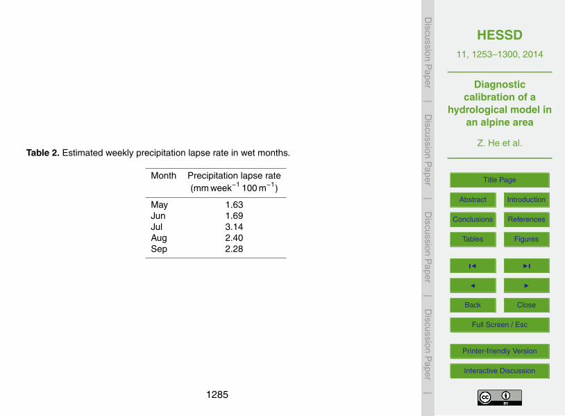
HESSD11, 1253–1300, 2014



Z. He et al.

Title Page



Tables Figures

J I

J I

Back Close

Full Screen / Esc



Discussion

Paper

|D

iscussionP

aper|

Discussion

Paper

|D

iscussionP

aper|

Table 2. Estimated weekly precipitation lapse rate in wet months.

Month Precipitation lapse rate(mm week−1 100 m−1)

May 1.63Jun 1.69Jul 3.14Aug 2.40Sep 2.28

1285





HESSD11, 1253–1300, 2014



Z. He et al.

Title Page



Tables Figures

J I

J I

Back Close

Full Screen / Esc



Discussion

Paper

|D

iscussionP

aper|

Discussion

Paper

|D

iscussionP

aper|

Table 3. Parameter properties in the THREW model.

Category Symbol Unit Description Value

Subsurface K us m s−1 Saturated hydraulic conductivity for u zone 1.25×10−05

K ss m s−1 Saturated hydraulic conductivity for s zone 1.25×10−05

εu – Soil porosity value of u zone 4.80×10−01

εs – Soil porosity value of s zone 2.88×10−01

Ψa m Air entry value 2.50×10−01

µ – Soil pore size distribution index 2.00×10−01

KKA – Coefficient used to calculate subsurface flow 1.10×10+00

βk – Coefficient used to calculate unsaturated hydraulic con-ductivity

8.00×10−01

βΨ – Coefficient used to calculate matrix potential 2.50×10−01

αuvz – Spatial heterogeneous coefficient for flow velocity of

u zone1.03×10+00

αus – Spatial heterogeneous coefficient for flow flux betweenu zone and s zone

1.66×10+00

kb – Empirical coefficient used to estimate the potential crackvolume of soil layer

0.00×10+00

Routing nt – Manning roughness coefficient for hillslope, obtained fromthe literature according to land use and vegetation type

1.50×10−01

nr – Similar to nt, roughness coefficient for channel 3.00×10−01

αtr – Spatial heterogeneous coefficient for flow flux betweent zone and r zone

1.10×10−01

Infiltration αEFL – Spatial heterogeneous coefficient for exfiltration capacity 1.00×10+00

αIFL – Spatial heterogeneous coefficient for infiltration capacity 1.50×10+00

Interception Fmaxb m Ground surface depression storage capacity 0.00×10+00

αvb m Maximum rainfall depth a single leaf can intercept and hold 1.00×10−05

Evaporation kv – Ratio of potential evapotranspiration over potential evapo-ration

9.00×10−01

Storm-runoff B – Shape coefficient to calculate the saturation excess runoffarea from the Xin’anjiang model

Calibrated

WM m Spatial averaged tension water storage capacity in theXin’anjiang model

Calibrated

Melt GDDF mm ◦C−1 day−1 Degree per day factor used to calculate glacier melt in thetemperature-index model, which is subject to calibration

Calibrated

SDDF mm ◦C−1 day−1 Degree per day factor used to calculate snowmelt in thetemperature-index model, which is subject to calibration

Calibrated

1286





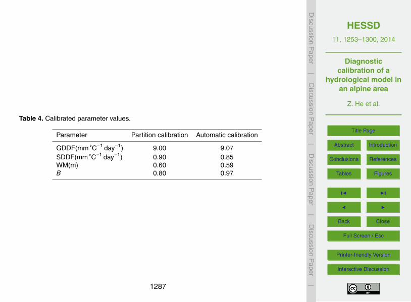
HESSD11, 1253–1300, 2014



Z. He et al.

Title Page



Tables Figures

J I

J I

Back Close

Full Screen / Esc



Discussion

Paper

|D

iscussionP

aper|

Discussion

Paper

|D

iscussionP

aper|

Table 4. Calibrated parameter values.

Parameter Partition calibration Automatic calibration

GDDF(mm ◦C−1 day−1) 9.00 9.07SDDF(mm ◦C−1 day−1) 0.90 0.85WM(m) 0.60 0.59B 0.80 0.97

1287





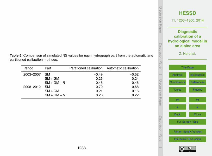
HESSD11, 1253–1300, 2014



Z. He et al.

Title Page



Tables Figures

J I

J I

Back Close

Full Screen / Esc



Discussion

Paper

|D

iscussionP

aper|

Discussion

Paper

|D

iscussionP

aper|

Table 5. Comparison of simulated NS values for each hydrograph part from the automatic andpartitioned calibration methods.

Period Part Partitioned calibration Automatic calibration

2003–2007 SM −0.49 −0.52SM+GM 0.26 0.24SM+GM+R 0.46 0.46

2008–2012 SM 0.70 0.68SM+GM 0.21 0.15SM+GM+R 0.23 0.22

1288





HESSD11, 1253–1300, 2014



Z. He et al.

Title Page



Tables Figures

J I

J I

Back Close

Full Screen / Esc



Discussion

Paper

|D

iscussionP

aper|

Discussion

Paper

|D

iscussionP

aper|

36

848

Figure 1. Location of the Tailan River basin in Xinjiang, China. Two automatic weather 849

stations (TG at 2381 m a.s.l. and XT at 2116 m a.s.l.) were set up in an upstream mountain 850

area in July, 2011. Additionally, the BT AWS (at 3950 m a.s.l.) located in the adjacent 851

catchment (Kumalak basin) was used to validate the estimated temperature lapse rates. The 852

Tailan Hydrologic Station (THS) has gauged streamflow data at the catchment outlet since 853

1957(b). Glacier coverage occupies approximately 33% of the total basin area (a). 854

Fig. 1. Location of the Tailan River basin in Xinjiang, China. Two automatic weather stations (TGat 2381 ma.s.l. and XT at 2116 ma.s.l.) were set up in an upstream mountain area in July 2011.Additionally, the BT AWS (at 3950 ma.s.l.) located in the adjacent catchment (Kumalak basin)was used to validate the estimated temperature lapse rates. The Tailan Hydrologic Station(THS) has gauged streamflow data at the catchment outlet since 1957 (b). Glacier coverageoccupies approximately 33 % of the total basin area (a).

1289





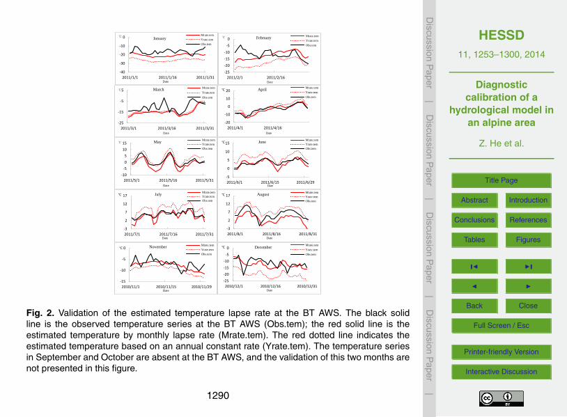
HESSD11, 1253–1300, 2014



Z. He et al.

Title Page



Tables Figures

J I

J I

Back Close

Full Screen / Esc



Discussion

Paper

|D

iscussionP

aper|

Discussion

Paper

|D

iscussionP

aper|

37

855

856

857

858

859 Figure 2. Validation of the estimated temperature lapse rate at the BT AWS. The black solid 860

line is the observed temperature series at the BT AWS (Obs.tem); the red solid line is the 861

estimated temperature by monthly lapse rate (Mrate.tem). The red dotted line indicates the 862

estimated temperature based on an annual constant rate (Yrate.tem). The temperature series in 863

September and October are absent at the BT AWS, and the validation of this two months are 864

not presented in this figure. 865

-40

-30

-20

-10

0

2011/1/1 2011/1/16 2011/1/31

Mrate.tem

Yrate.tem

Obs.tem

January℃

Date

-25

-20

-15

-10

-5

0

2011/2/1 2011/2/16

Mrate.tem

Yrate.tem

Obs.tem

February℃

Date

-25

-15

-5

5

2011/3/1 2011/3/16 2011/3/31

Mrate.tem

Yrate.tem

Obs.tem

March

Date

℃

-20

-10

0

10

20

2011/4/1 2011/4/16

Mrate.tem

Yrate.tem

Obs.tem

April℃

Date

-10

-5

0

5

10

15

2011/5/1 2011/5/16 2011/5/31

Mrate.tem

Yrate.tem

Obs.tem

May℃

Date

-5

0

5

10

15

2011/6/1 2011/6/15 2011/6/29

Mrate.tem

Yrate.tem

Obs.tem

June℃

Date

-3

2

7

12

17

2011/7/1 2011/7/16 2011/7/31

Mrate.tem

Yrate.tem

Obs.tem

July℃

Date

-3

2

7

12

17

2011/8/1 2011/8/16 2011/8/31

Mrate.tem

Yrate.tem

Obs.tem

August℃

Date

-15

-10

-5

0

2010/11/1 2010/11/15 2010/11/29

Mrate.tem

Yrate.tem

Obs.tem

November℃

Date

-25

-20

-15

-10

-5

0

2010/12/1 2010/12/16 2010/12/31

Mrate.tem

Yrate.tem

Obs.tem

December

Date

℃

Fig. 2. Validation of the estimated temperature lapse rate at the BT AWS. The black solidline is the observed temperature series at the BT AWS (Obs.tem); the red solid line is theestimated temperature by monthly lapse rate (Mrate.tem). The red dotted line indicates theestimated temperature based on an annual constant rate (Yrate.tem). The temperature seriesin September and October are absent at the BT AWS, and the validation of this two months arenot presented in this figure.

1290





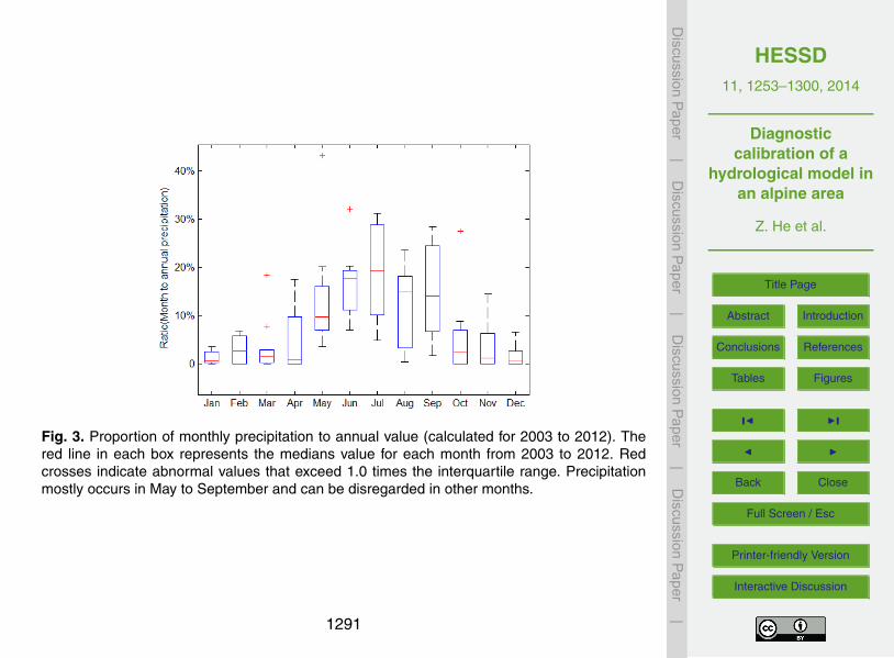
HESSD11, 1253–1300, 2014



Z. He et al.

Title Page



Tables Figures

J I

J I

Back Close

Full Screen / Esc



Discussion

Paper

|D

iscussionP

aper|

Discussion

Paper

|D

iscussionP

aper|

38

866

Figure 3. Proportion of monthly precipitation to annual value (calculated for 2003 to 2012). 867

The red line in each box represents the medians value for each month from 2003 to 2012. Red 868

crosses indicate abnormal values that exceed 1.0 times the interquartile range. Precipitation 869

mostly occurs in May to September and can be disregarded in other months. 870

Fig. 3. Proportion of monthly precipitation to annual value (calculated for 2003 to 2012). Thered line in each box represents the medians value for each month from 2003 to 2012. Redcrosses indicate abnormal values that exceed 1.0 times the interquartile range. Precipitationmostly occurs in May to September and can be disregarded in other months.

1291





HESSD11, 1253–1300, 2014



Z. He et al.

Title Page



Tables Figures

J I

J I

Back Close

Full Screen / Esc



Discussion

Paper

|D

iscussionP

aper|

Discussion

Paper

|D

iscussionP

aper|

39

871 Figure 4. Filtered MODIS eight-day snow-cover products in 2004-2005. mod is the snow 872 cover area from MOD10A2 products, while myd is MYD10A2 products. combined is the 873

combined result from step 1, spatial-comb from step 2 and temporal-comb from step 3. See 874 Sect. 2.2.3 for details. 875

Fig. 4. Filtered MODIS eight-day snow-cover products in 2004–2005. mod is the snow coverarea from MOD10A2 products, while myd is MYD10A2 products. combined is the combinedresult from step 1, spatial-comb from step 2 and temporal-comb from step 3. See Sect. 2.2.3for details.

1292





HESSD11, 1253–1300, 2014



Z. He et al.

Title Page



Tables Figures

J I

J I

Back Close

Full Screen / Esc



Discussion

Paper

|D

iscussionP

aper|

Discussion

Paper

|D

iscussionP

aper|

40

876 Figure 5a. Cumulative monthly snowmelt area distribution by elevation for 2003 to 2012. The 877

snowmelt area in December, January and February is zero and is not shown in this figure. 878

0

1000

2000

3000

4000

5000

6000

7000

0 1000 2000 3000 4000 5000 6000

Mar

Jun

Apr

May

Jul

Aug

Sep

Oct

Nov

Elevation (m)

Mel

t A

rea(

km

2)

Fig. 5a. Cumulative monthly snowmelt area distribution by elevation for 2003 to 2012. Thesnowmelt area in December, January and February is zero and is not shown in this figure.

1293





HESSD11, 1253–1300, 2014



Z. He et al.

Title Page



Tables Figures

J I

J I

Back Close

Full Screen / Esc



Discussion

Paper

|D

iscussionP

aper|

Discussion

Paper

|D

iscussionP

aper|

41

879 Figure 5b. Cumulative monthly glacier melt area distribution by elevation for 2003 to 2012. 880

The glacier melt area in November, December, January and February is zero and is not shown 881 in this figure. 882

883

0

2000

4000

6000

8000

10000

12000

14000

16000

0 1000 2000 3000 4000 5000 6000

Mar

Apr

May

Jun

Jul

Aug

Sep

Oct

Elevation (m)

Mel

t A

rea(

km

2)

Fig. 5b. Cumulative monthly glacier melt area distribution by elevation for 2003 to 2012. Theglacier melt area in November, December, January and February is zero and is not shown inthis figure.

1294





HESSD11, 1253–1300, 2014



Z. He et al.

Title Page



Tables Figures

J I

J I

Back Close

Full Screen / Esc



Discussion

Paper

|D

iscussionP

aper|

Discussion

Paper

|D

iscussionP

aper|

42

884 Figure 6. Area ratio of different land cover types for 2003-2012 in the TRB. 885

0%

10%

20%

30%

40%

50%

60%

70%

80%

90%

100%

2003 2004 2005 2006 2007 2008 2009 2010 2011 2012

Water

Woody plants

Shrub

Grass

Snow/Ice

Bare land

Year

Are

a R

atio

Fig. 6. Area ratio of different land cover types for 2003–2012 in the TRB.

1295





HESSD11, 1253–1300, 2014



Z. He et al.

Title Page



Tables Figures

J I

J I

Back Close

Full Screen / Esc



Discussion

Paper

|D

iscussionP

aper|

Discussion

Paper

|D

iscussionP

aper|

43

886

Figure 7. Hydrograph partition of 2003. 887 Fig. 7. Hydrograph partition of 2003.

1296





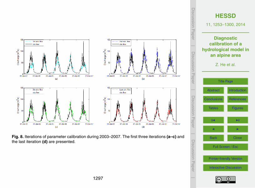
HESSD11, 1253–1300, 2014



Z. He et al.

Title Page



Tables Figures

J I

J I

Back Close

Full Screen / Esc



Discussion

Paper

|D

iscussionP

aper|

Discussion

Paper

|D

iscussionP

aper|

44

888

Figure 8. Iterations of parameter calibration during 2003-2007. The first three iterations (a-c) 889

and the last iteration (d) are presented. 890

Fig. 8. Iterations of parameter calibration during 2003–2007. The first three iterations (a–c) andthe last iteration (d) are presented.

1297





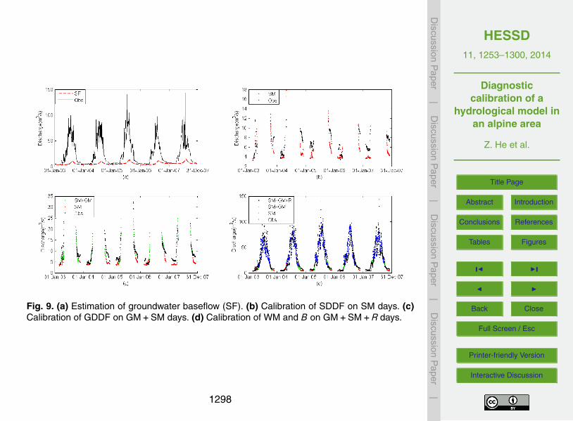
HESSD11, 1253–1300, 2014



Z. He et al.

Title Page



Tables Figures

J I

J I

Back Close

Full Screen / Esc



Discussion

Paper

|D

iscussionP

aper|

Discussion

Paper

|D

iscussionP

aper|

45

891

Figure 9. (a) Estimation of groundwater baseflow (SF). (b) Calibration of SDDF on SM days. 892

(c) Calibration of GDDF on GM+SM days. (d) Calibration of WM and B on GM+SM+R 893

days. 894

Fig. 9. (a) Estimation of groundwater baseflow (SF). (b) Calibration of SDDF on SM days. (c)Calibration of GDDF on GM+SM days. (d) Calibration of WM and B on GM+SM+R days.

1298





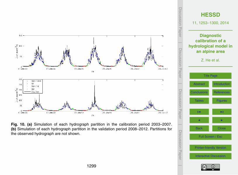
HESSD11, 1253–1300, 2014



Z. He et al.

Title Page



Tables Figures

J I

J I

Back Close

Full Screen / Esc



Discussion

Paper

|D

iscussionP

aper|

Discussion

Paper

|D

iscussionP

aper|

46

895

Figure 10. (a) Simulation of each hydrograph partition in the calibration period 2003-2007. (b) 896

Simulation of each hydrograph partition in the validation period 2008-2012. Partitions for the 897

observed hydrograph are not shown. 898

Fig. 10. (a) Simulation of each hydrograph partition in the calibration period 2003–2007.(b) Simulation of each hydrograph partition in the validation period 2008–2012. Partitions forthe observed hydrograph are not shown.

1299





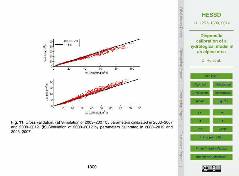
HESSD11, 1253–1300, 2014



Z. He et al.

Title Page



Tables Figures

J I

J I

Back Close

Full Screen / Esc



Discussion

Paper

|D

iscussionP

aper|

Discussion

Paper

|D

iscussionP

aper|

47

899

Figure 11. Cross validation. (a) Simulation of 2003-2007 by parameters calibrated in 900

2003-2007 and 2008-2012. (b) Simulation of 2008-2012 by parameters calibrated in 901

2008-2012 and 2003-2007. 902

Fig. 11. Cross validation. (a) Simulation of 2003–2007 by parameters calibrated in 2003–2007and 2008–2012. (b) Simulation of 2008–2012 by parameters calibrated in 2008–2012 and2003–2007.

1300





Documents

Diagnostic calibration of a hydrological model in an … 11, 1253–1300, 2014 Diagnostic calibration of a hydrological model in an alpine area Z. He et al. Title Page Abstract Introduction