Application of Bayesian Inference to Operational Risk Management
Yuji Yasuda (Doctoral Program in Quantitative Finance and Management)
Advised by Professor Isao Shoji
Submitted to the Graduate School of
System and Information Engineering
in Partial Fulfillment of the Requirements
for the Degree of Master of Finance
University of Tsukuba
January 2003
Application of Bayesian Inference to Operational Risk Management
Yuji Yasuda
Abstract
Bayesian inference that is able to combine statistical measurement
approach and scenario analysis is effective exceedingly for measuring
operational risk. In choosing the prior distribution, taking
indicators that may be predictive of the risk of future losses, external
circumstance and so forth into consideration makes it possible to
obtain more realistic risk amount, this process itself is an important
for enhancing operational risk management. This paper proposes
the examples of application of Bayesian inference to banking
practices.
Keywords: Operational risk, Bayesian inference, Prior distribution.

Acknowledgement
I am deeply grateful to my academic advisor, Professor Isao Shoji for his
encouragement and constructive comments. I also thank the member of Shoji
Laboratory and all my friends for their support.
Finally, I appreciate the Bank of Tokyo-Mitsubishi, Ltd. that gave me a
good opportunity that I have studied at the University of Tsukuba.
Contents
Introduction ····· · · · · · · · · · · · · · · · · · · · · · · · · · · · · · · · · · · · · · · · · · · · · · · · · · · · · · · · · · · · · · · · · · 1
1. Background ····· · · · · · · · · · · · · · · · · · · · · · · · · · · · · · · · · · · · · · · · · · · · · · · · · · · · · · · · · · · · · · · 3
1.1. What is Operational Risk? ·· · · · · · · · · · · · · · · · · · · · · · · · · · · · · · · · · · · · · · · · · · · · · · · · · · · · · · · 3
1.2. Why is It Important?· · · · · · · · · · · · · · · · · · · · · · · · · · · · · · · · · · · · · · · · · · · · · · · · · · · · · · · · · · · · · · · 5
1.3. Why is Measuring It Necessary? ·· · · · · · · · · · · · · · · · · · · · · · · · · · · · · · · · · · · · · · · · · · · · · · · 9
2. The Concept of Measuring Operational Risk···· · · · · · · · · · · · · · · · · · 12
2.1. Top-Down Method·· · · · · · · · · · · · · · · · · · · · · · · · · · · · · · · · · · · · · · · · · · · · · · · · · · · · · · · · · · · · · · · 12
2.2. Bottom-Up Method ·· · · · · · · · · · · · · · · · · · · · · · · · · · · · · · · · · · · · · · · · · · · · · · · · · · · · · · · · · · · · · · 14
3. Application of Bayesian Inference ···· · · · · · · · · · · · · · · · · · · · · · · · · · · · · · · · 18
3.1. What is Bayesian Inference?·· · · · · · · · · · · · · · · · · · · · · · · · · · · · · · · · · · · · · · · · · · · · · · · · · · · · 18
3.2. Natural Conjugate Prior Distribution·· · · · · · · · · · · · · · · · · · · · · · · · · · · · · · · · · · · · · · · · 21
3.3. Advantages of Bayesian Inference·· · · · · · · · · · · · · · · · · · · · · · · · · · · · · · · · · · · · · · · · · · · · 26
4. Examples of Application to Banking Practices ···· · · · · · · · · · · · · · · · 28
4.1. Operations Error Rate · · · · · · · · · · · · · · · · · · · · · · · · · · · · · · · · · · · · · · · · · · · · · · · · · · · · · · · · · · · · 28
4.2. Number of Operations Loss Events · · · · · · · · · · · · · · · · · · · · · · · · · · · · · · · · · · · · · · · · · · · 30
4.3. Severity of Operations Loss Event· · · · · · · · · · · · · · · · · · · · · · · · · · · · · · · · · · · · · · · · · · · · · 32
4.4. Simulation of Risk Amount ·· · · · · · · · · · · · · · · · · · · · · · · · · · · · · · · · · · · · · · · · · · · · · · · · · · · · 33
4.5. Profitability Judgment·· · · · · · · · · · · · · · · · · · · · · · · · · · · · · · · · · · · · · · · · · · · · · · · · · · · · · · · · · · · 35
5. Discussions ···· · · · · · · · · · · · · · · · · · · · · · · · · · · · · · · · · · · · · · · · · · · · · · · · · · · · · · · · · · · · · · · 36
References···· · · · · · · · · · · · · · · · · · · · · · · · · · · · · · · · · · · · · · · · · · · · · · · · · · · · · · · · · · · · · · · · · · · · · 38

1
Introduction
Rapid and extensive changes in the banking environment make
operational risk management more important. These changes result from
economic and financial globalization and continuing advances in information
technology. The need to manage operational risk through measuring
methods becomes increasingly urgent with each passing year. The Basel
Committee is currently working on new BIS rules to include operational risk
within capital adequacy guidelines along with market and credit risk.
Furthermore, it will become more and more important in the future to control
risk along with cost reduction as low-cost operation is enhanced through
continuous rationalization of bank management.
There are two main methods in measuring operational risk: statistical
measurement approach and scenario analysis. Statistical measurement
approach is to be performed to the same standard as for market risk and credit
risk, statistically measure the risk based on historical data on frequency of loss
occurrence, size of loss and so forth. On the other hand, under scenario
approach, as for events with low frequency and high severity, losses would be
estimated based on scenarios, with reference to external data and events that
occurred at other banks.
However, if banks measure risk based only on past event data, they might
not capture those material potential events with “low frequency and high
severity” and, likewise, will not capture the future impact of the changing
2
environment (both internally and externally) on future operational losses.
Scenario analysis tends to be less objective than statistical measurement
approach.
So, we propose we apply Bayesian inference to measuring operational risk.
Bayesian inference combines statistical measurement approach and scenario
analysis. For measuring market risk and insurance, the Bayesian analysis of
extreme value data has been developed by Kotz and Nadarajah (2000), and
Smith (2000). The idea of Bayesian network is applicable to only settlement
risk. For operational risk management, Cruz (2002) just mentioned Bayesian
techniques in his operational risk textbook briefly. So, we introduce the
examples of application of Bayesian inference to operational risk management
in view of banking practices.
By applying Bayesian inference, we can use both data as likelihood, and
non-data information as prior distribution. Predictive indicator and
qualitative data result can be used for measuring.
This paper aims to provide reader with possible solutions, or at least hints.
This paper is organized as follows. We review the operational risk in section
1. Section 2 summarizes the methods of measuring operational risk proposed
until now. The concept of Bayesian inference is described in Section 3. In
section 4, the examples of applications for business practices are presented and
discussions follow in section 5.
3
1. Background
1.1. What is Operational Risk?
Operational risk was a term that has a variety of meanings within the
banks. Some banks defined operational risk as a non-measurable risk. A
universal definition has not yet been established, but there has been a high
degree of convergence during the past few years.
In January 2001, the Basel Committee on Banking Supervision, which
formulates broad supervisory standards and guidelines and recommends
statements of best practice, defined ‘operational risk’ as: ‘the risk of loss
resulting from inadequate or failed internal processes, people and systems or
from external events’. This definition was adopted from industry as part of
the Committee’s work in developing a minimum regulatory capital charge for
it.
This definition includes operations risk, IT risk and legal risk. Examples
of operational risk event include the following:
Execution, delivery and process management (data entry errors,
collateral management failures, incomplete legal documentation,
unapproved access given to client account, non-client counterpatry
misperformance, vendor disputes, etc.)
System failure (hardware and software failures, telecommunication
problems, utility outage, etc.)
4
Internal fraud (intentional misreporting of positions, employee theft,
insider trading on an employee’s own account, etc.)
External fraud (robbery, forgery, cheque kiting, damage from computer
hacking, etc)
Client, products and business practices (fiduciary breaches, misuse of
confidential customer information, improper trading activities on the
bank’s account, money laundering, sale of unauthorized products, etc.)
Damage to physical assets (terrorism, vandalism, earthquakes, fires
floods, etc.)
The Basel Committee’s definition excludes strategic, reputation and
systemic risk. They are not suitable for capturing and control based on
measuring risk at present. This issue should always be revisited in the future
in accordance with development of management environment and business
structure.
5
1.2. Why is It Important?
(1) Substantial Loss Events
The term “operational risk” was mentioned for the first time after the
infamous Barings bankruptcy event in 1995. Barings lost $1.9 billion
through unauthorized trading by their "star" trader, Nick Leeson.
Breakdowns in fundamental controls can be attributed to these losses, as
Leeson's activities went unnoticed until it was too late.
Also, the Daiwa Bank’s rogue trader, Toshihide Igushi, lost $1.1 billion
through trading in US treasury bonds. The trades took place unnoticed over
a long period of time, in fact 11 years from 1984 to 1995. The trader covered
up the trading losses by falsifying assets supposedly owned by the bank. It is
clear that through these actions the trader was in effective control of both front
and back offices. This is a fundamental violation of any risk management
strategy. Unlike Barings collapse, Daiwa survived although the incident cost
them one seventh of their capital base. And US regulators prohibited them
from continuing their operations there, an unprecedented move.
Recently, the terrorist attacks on the United States on September 11, 2001,
damaged many banks’ physical assets immensely. The computer systems
problems and operational confusion, such as ATM services problems and
delays in automatic debit transactions, in connection with the launching of
Mizuho Corporate Bank and Mizuho Bank in April 2002, is fresh in our
memory.
6
(2) Complexity of Bank’s Operations
Over a few decades, banks have developed, and have capitalized on, new
business opportunities given advances made in IT, deregulation, and
globalization. Also, sophistication of financial technology has been growing.
As the result of the faster pace of change in the complexity of their operations,
the operational risks that banks face today have become more complex and
diverse than ever before. Examples of these new and growing risks faced by
banks include:
Growth of e-commerce brings with it potential risks (e.g., external
fraud and system security issues) that are not yet fully understood;
Large-scale mergers, de-mergers and consolidations test the viability of
new or newly integrated systems;
If not properly controlled, the use of more highly automated
technology has the potential to transform risk from manual processing
errors to system failure risk, as greater reliance is placed on globally
integrated systems; and
Banks may engage in risk mitigation techniques (e.g., collateral, credit
derivatives, netting arrangements and asset securitizations) to
optimize their exposure to market risk and credit risk, but which in
turn may produce other forms of risk.
7
(3) The New Basel Capital Accord
The Basel Committee on Banking Supervision of the Bank for
International Settlements sets BIS guidelines that prescribe capital adequacy
standards for all internationally active banks.
More than a decade has passed since the Basel Committee introduced its
1988 Capital Accord. The business of banking, risk management practices,
supervisory approaches, and financial markets each have undergone
significant transformation since then. In January 2001, the Committee issued
a proposal for a New Basel Accord. The proposal has three core elements:
required regulatory capital in line with the risks at each financial institution;
supervisory reviews by national banking regulators, and market discipline
through the disclosure of information. The Committee believes that three
“pillars” will collectively ensure the stability and soundness of financial
systems.
In response to the growing need for a system to cope with these
operational risks, the Basel Committee is currently working on new BIS rules
to include operational risk within capital adequacy guidelines along with
market and credit risk. The 1988 Accord set a capital requirement simply in
terms of credit risk (the principal risk for banks), though the overall capital
requirement (i.e., the 8% minimum ratio) was intended to cover other risks as
well. In 1996, market risk exposures were removed and given separate
capital charges. In its attempt to introduce greater credit risk sensitivity, the
Committee has been working with the industry to develop a suitable capital
8
charge for operational risk.
The new regulations themselves will reflect the nature of risks at banks
more closely. To calculate the regulatory capital, the Committee has offered a
menu of options from which banks can choose not only market risk, where the
menu approach has been implemented since 1998, but also for credit risk and
operational risk in the proposed framework. Under this framework, banks
can choose calculate their own required regulatory capital based on their own
risk profiles and risk management methodology. Therefore, banks have
started work to conform to the proposed regulations. This includes the
selection of a more advanced approach in the proposed menu in line with their
risk profiles.
The Committee, in discussions with the industry, is currently finalizing
the proposal. The new regulations are expected to become effective in 2006.
9
1.3. Why is Measuring It Necessary?
Operational risk in the past used to control based on qualitative risk
management practices involving checklist and operations manual. But banks
have found limits to traditional qualitative operational risk management.
Measuring risk is an effective tool for capturing and controlling it. The main
reasons why banks try to measure operational risk are following:
(1) Adequacy of Required Economic Capital for Risk
As market risk and credit risk measurement methods have been developed,
large banks have, in turn, established a capital allocation system. By
optimizing capital allocation, banks aim to maximize return after deducing cost
of capital and risk-adjusted performance measurement, which assess their
profitability and efficiency relative to risks.
The capital allocation system sets the amount of capital allowed to be
placed at risk by each our business units. The level of risk is then controlled
and managed so as to remain within that allocation. Each business units
must take risks within their capital adequacy. The capital allocated by this
system seeks to cover all risks including operational risks. Thus, it is
inevitable for banks to allocate their economic capital to operational risk
explicitly.
Capturing risk on an integrated basis by measuring each risk according to
a common standard makes different types of risk comparable with each other
10
and thus leads to an effective and efficient use of management resources.
(2) Performance Evaluation
It is important to give employees the incentives to enhance risk
management through various methods such as performance indicators. It is
commonly seen in practice, however, that employees tend to focus on ways to
increase return rather than performance indicators such as return on equity
(ROE). ROE could be based on measured risk, depending on the balance
between risk taking and risk management. Thus, banks seek to allocate
economic capital to operational risk based on risk measurement and results of
risk assessment, so employees have an incentive to improve risk management.
The improvement, which turns out to be measured, reduces the allocated
capital to their operational risk as their performance evaluation improves.
(3) Internal Control Framework
Some banks seek to establish a basis for effective and efficient internal
control measures. Subjective judgments on internal control, however, tend to
misguide the board of directors and senior managers with wrong priorities in
enhancing operational risk management. Operational risk measurement
enables banks to establish criteria of objectivity and comparability in
prioritizing risk control among different business lines and risk categories, in
order to supplement internal control in a more robust way. The result of
operational risk measurement can be fed back to each business unit such as a
11
branch at section level and serve as an incentive to improve internal control
such as the revision of operating procedures.
(4) Criterion for Use of Insurance
It is worthwhile to keep abreast of effective risk transfer methods such as
insurance or ART (Alternative Risk Transfer). Insurance companies start to
supply not only traditional BBB (Bankers Blanket Bonds) but also more
comprehensive insurance products which cover a wider range of operational
risks faced by banks. Measurement of operational risk will serve as an
important criterion for determining which is more advantageous in light of the
cost of capital, maintaining capital or buying insurance.

12
2. The Concept of Measuring Operational Risk
There are both Top-down and Bottom-up methods in measuring
operational risk. At present, several kinds of measurement methods are
being developed and no industry standard has yet emerged. The details of
these methods can be seen in Hiwatashi and Ashida (2002) and Marcelo G.
Cruz (2002).
2.1. Top-Down Method
Top-down method seeks to estimate operational risk on a macro basis
without identifying events or causes of losses. Table 1 shows the examples of
Top-down method. In Top-down method, the total amount or change of
profits or expense etc. derived from financial data in the balance sheet and
profit & loss statement is converted to risk amount.
Although this method enables easy capturing of the overall risk, it is
difficult in this way to determine incentives for risk mitigation by identifying
the areas needing improvement. It does not lead to an appropriate capturing
of risk according to the circumstances nor serves as adequate information for
market participants because it usually applies one uniform set of
multiplication factors regardless of the differences between countries in
accounting systems, employment practice, and the level of expectation from
customers for services provided by banks and so forth.
13
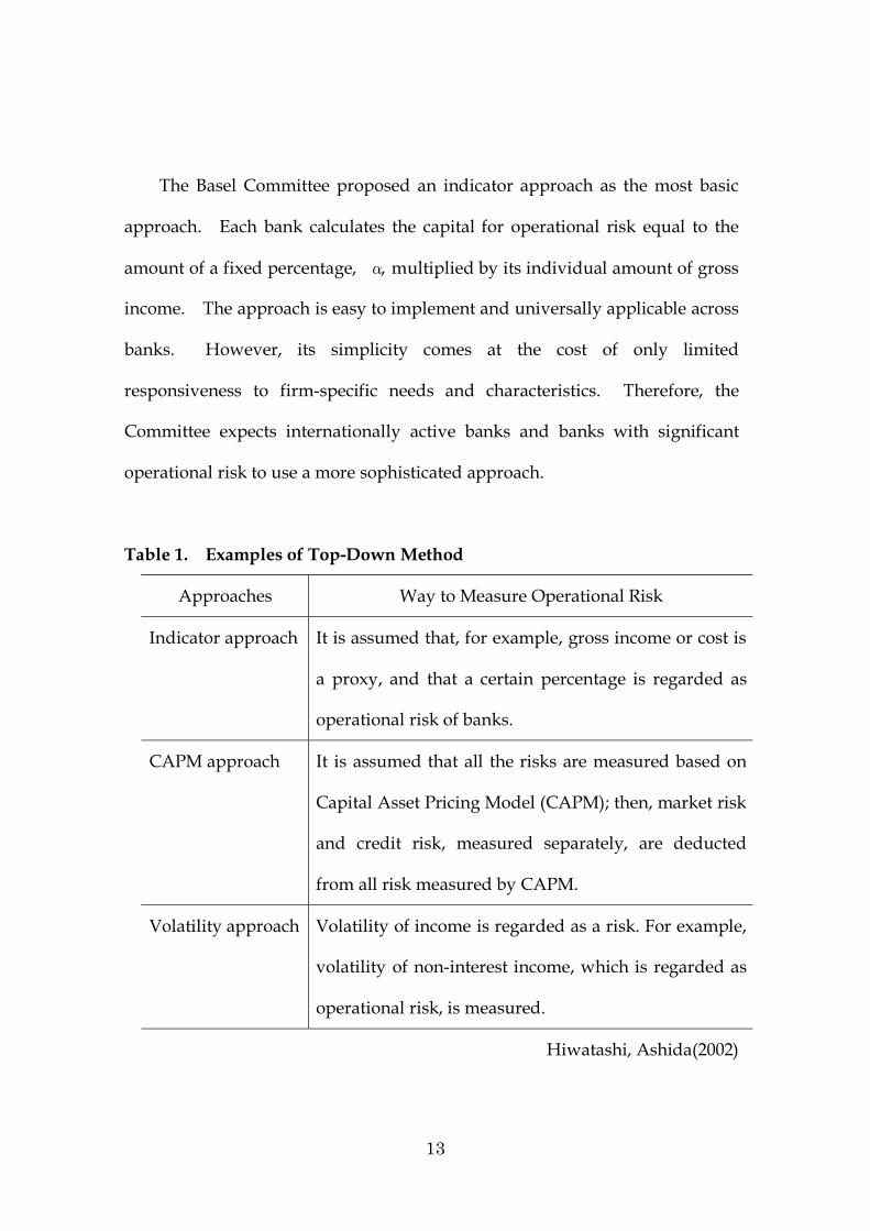
The Basel Committee proposed an indicator approach as the most basic
approach. Each bank calculates the capital for operational risk equal to the
amount of a fixed percentage, α, multiplied by its individual amount of gross
income. The approach is easy to implement and universally applicable across
banks. However, its simplicity comes at the cost of only limited
responsiveness to firm-specific needs and characteristics. Therefore, the
Committee expects internationally active banks and banks with significant
operational risk to use a more sophisticated approach.
Table 1. Examples of Top-Down Method
Approaches Way to Measure Operational Risk
Indicator approach It is assumed that, for example, gross income or cost is
a proxy, and that a certain percentage is regarded as
operational risk of banks.
CAPM approach It is assumed that all the risks are measured based on
Capital Asset Pricing Model (CAPM); then, market risk
and credit risk, measured separately, are deducted
from all risk measured by CAPM.
Volatility approach Volatility of income is regarded as a risk. For example,
volatility of non-interest income, which is regarded as
operational risk, is measured.
Hiwatashi, Ashida(2002)
14
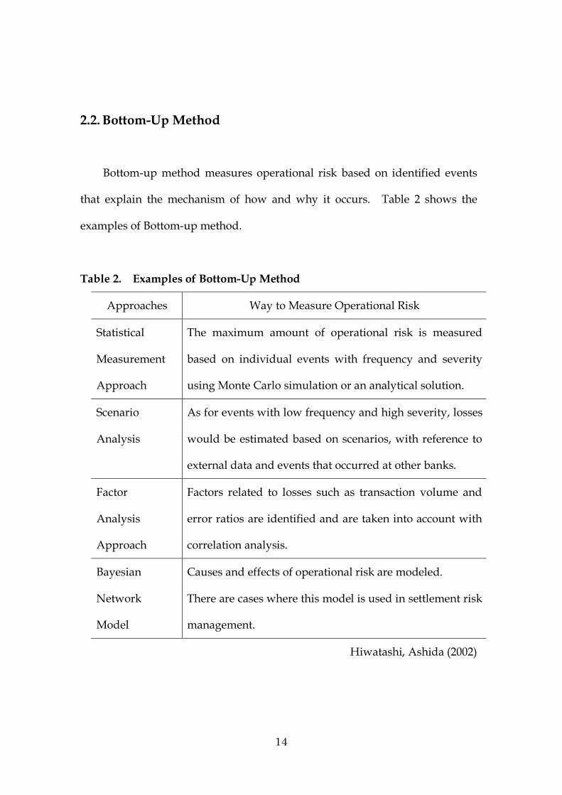
2.2. Bottom-Up Method
Bottom-up method measures operational risk based on identified events
that explain the mechanism of how and why it occurs. Table 2 shows the
examples of Bottom-up method.
Table 2. Examples of Bottom-Up Method
Approaches Way to Measure Operational Risk
Statistical
Measurement
Approach
The maximum amount of operational risk is measured
based on individual events with frequency and severity
using Monte Carlo simulation or an analytical solution.
Scenario
Analysis
As for events with low frequency and high severity, losses
would be estimated based on scenarios, with reference to
external data and events that occurred at other banks.
Factor
Analysis
Approach
Factors related to losses such as transaction volume and
error ratios are identified and are taken into account with
correlation analysis.
Bayesian
Network
Model
Causes and effects of operational risk are modeled.
There are cases where this model is used in settlement risk
management.
Hiwatashi, Ashida (2002)
15
This method enables the analysis of risk factors and serves as an effective
incentive for reduction operational cost and mitigation of operational risk
including the review of operational work flows though it required complicated
analysis of risk by business line.
The following two approaches are used widely in Bottom-up method:
(1) Statistical Measurement Approach
Under the statistical measurement approach, a bank, using its internal
data, estimates two probability distribution functions for each business line
and risk type; one on single event impact (severity) and the other on event
frequency for the next one year.
Having calculated separately both the severity and frequency processes,
we need to combine them into one aggregated loss distribution that allows us
to predict figure for the operational losses with a degree of confidence using
Monte Carlo simulation or an analytical solution.
The idea behind statistical measurement approach is as follows:
Measurement of operational risk should be performed to the same standard as
for market risk and credit risk. They should also be comparable with each
other to ensure control on an integrated basis. Market risk and credit risk
have been statistically measured based on the analysis of historical data on the
market and actual loss. As for the capital charge on operational risk, it will
confirm to the objective of risk management, i.e. precise capturing risk, and
will lead to enhancement of risk management capabilities of banks to
16
statistically measure the risk in the bottom-up methods based on historical
data on frequency of loss occurrence, size of loss and so forth.
However, if banks measure risk based only on past event data, they might
not capture those material potential events with “low frequency and high
severity” and, likewise, will not capture the future impact of the changing
environment (both internally and externally) on future operational losses. In
other words, the historical loss observation may not always fully capture a
bank’s true profile, especially when the bank does not experience substantial
loss events during the observation period.
To supplement the limits of an internal data with external data may very
useful. However, in the course of implementing them, they may face the
challenging risk management issue of mapping that external data into an
internal database with differing transaction volume.
(2) Scenario Analysis
Under scenario analysis, first, banks identify not only the past events of
operational risk but also its potential events based on, for example, the past
events which happened in other banks and the impact of changes in
environments on their operations flows. Second, banks estimate frequency
and severity of these events identified by analyzing causes of these events and
factors of causing losses and expanding loss amounts. In this process, a
coordinated risk management department in operational risk takes an
initiative in giving questionnaires to business lines so that common
17
understanding and challenging issues can be shared between the risk
management department and business lines. External data contribute to the
development of robust scenario analyses.
Scenario analysis is flexible and effective way of making good use of
information obtained by risk assessment, risk mapping, key risk indicators,
and scorecards. In risk assessment, bank’s operation and activities are
assessed against a menu of potential operational risk vulnerabilities. This
process often incorporates checklists and/or workshops to identify the
strengths and weaknesses of the operational risk environment. In risk
mapping, various business units, organizational functions or process flows are
mapped by risk type. This exercise can reveal areas of weakness and help
prioritize subsequent management action. Key risk indicators can provide
insight into bank’s risk position. Scorecards provide a means of translating
qualitative assessments into quantitative metric that give a relative ranking of
different types of operational risk exposures.
But scenario analysis tends to be less objective than statistical
measurement approach. Risk amount varies strikingly by which scenarios
are adopted. The opinion that it is just tool for supplement statistical is
insisted considerably.
18
3. Application of Bayesian Inference
In short, it is necessary to measure operational risk based not only on
historical data, but also scenario data with forward looking approaches, given
the rapid change in environment surrounding the banking industry.
So, we propose to apply Bayesian inference to measuring operational risk.
Bayesian inference combines statistical measurement approach and scenario
analysis. Cruz (2002) introduced Bayesian techniques in his operational risk
textbook briefly, too. But he only introduced quite simple concept, we focus a
point of view from banking practices.
3.1. What is Bayesian Inference?
(1) Bayes’ Theorem
Suppose that )...,,( 1 nxx=z is a vector of n observations whose
probability distribution p(z| θ) depends on the values of k parameters
)...,,( 1 kθθ=θ . Suppose also that θ itself has a probability distribution p(θ).
Then,
)()|(),()()|( zzzz ppppp θθθθ == (1)
Given the observed data z, the conditional distribution of θ is
)()()|()|( z
zzp
ppp θθθ = (2)
Also, we can write

19
∑
∫=== −
discrete:)()|(continuous:)()|(
)]|([)( 1
θθθθθθθ
θppdpp
cpp zzzz E (3)
where the sum or the integral is taken over the admissible range of θ, and
where E[f( θ)] is the mathematical expectation of f(θ) with respect to the
distribution p(θ). Thus we may write (2) alternatively as
)()|()|( θθθ pcpp zz = . (4)
The statement of (2), or its equivalent (4), is usually referred to as Bayes’
theorem. In this expression, p(θ), which tells us what is known about θ
without knowledge of the data, is called prior distribution of θ, or the
distribution of θ a priori. Correspondingly, p(θ|z), which tells us what is
known about θ given knowledge of data, is called the posterior distribution
of θ given z, or the distribution of θ a posteriori. The quantity c is merely
a “normalizing” constant necessary to ensure that the posterior distribution
p( θ|z) integrates or sums to one.
(2) Likelihood Function
Now given the data z, p(z|θ) in (4) may be regarded as a function not of
z but of θ. It is called the likelihood function of θ for given z and can be
written l(θ|z). We can thus write Bayes’ formula as
)()|()|( θθθ plp zz = . (5)
In other words, then, Bayes’ theorem tells us that the probability
distribution for θ posterior to the data z is proportional to the product of the
distribution for θ prior to the data and the likelihood for θ given z . That
20
is,
posterior distribution ∝ likelihood × prior distribution.
Bayesian inference is a method based on above general equation. By
Bayesian inference, we can take our earlier practical experience into account
explicitly. Also, we often obtain shorter confidence intervals using proper prior
distributions than we could obtain if we ignored out practical experience.
(3) Point Estimator
The posterior distribution shows the distribution of parameterθ, not the
point estimator. A point estimator of parameter of a distribution, is often take
to be the mean of the posterior distribution ofθ. This is because the posterior
mean minimizes the mean quadratic loss function in a decision-theoretic
context. Other loss function would imply other Bayesian estimator. An
absolute error loss function implies a posterior median estimator; for an
unspecified loss function we sometimes use the posterior mode.
21
3.2. Natural Conjugate Prior Distribution
Conjugacy is formally defined as follows. If F is a class of sampling
distributions p(z|θ), and P is a class of prior distribution for θ, then the class
P is conjugate for F if
PpandFpallforPp ∈⋅∈⋅∈ )()|()|( θθ z . (6)
This definition is formally vague since if we choose P as the class of all
distributions, then P is always conjugate no matter what class of sampling
distributions is used. So, we think natural conjugate families, which arise by
taking P to be the set of all densities having the same functional form as the
likelihood. Conjugate prior distributions have the practical advantage of
being interpretable as additional data in addition to computational
convenience.
(1) Bernoulli Trials
Let there be n independent trials of an experiment in which there are only
two possible outcomes on each trial, labeled ‘success’ or ‘failure’, data xi(i=1,
…, n), each of which is either 1 or 0. Let θ denote the probability of success
on a single trial and take )...,,( 1 nxx=z . The likelihood function is binomial;
∑−∑= − ii xnxl )1()|( θθθ z . (7)
If θ were the random variable, l(θ|z) would look like a beta distribution.
But we don’t want the beta prior family to depend upon sample data, so we
use arbitrary parameters (α, β), and we norm the density to make it proper, to

22
get beta prior density,
0,0)1(),(
1)( 11 >>−= −− βαθθβα
θ βα
Bw . (8)
Now we use out prior beliefs to assess the hyperparameters α and β,
which are the parameters of the prior distribution, that is, having fixed the
family of priors as the beta distribution, only (α, β) remain unknown. We do
not have to assess the entire prior distribution.
An additional mathematical convenience arises in computing the posterior.
Since the posterior density is proportional to the likelihood times the prior, in
this case a beta prior, the posterior density is given by
])1([])1([)|( 11 −−− −−∝ ∑∑ βα θθθθθ ii xnxw z
∑∑ −−+−+ −∝ 11 )1()|( ii xnxw βα θθθ z , (9)
a beta posterior.
In practice, we choose hyperparameters α, β using these equation that
E(θ)= α/( α+ β)、V( θ)= αβ/( α+ β) 2 ( α+ β+1)、Mode( θ)=( α-1)/(α+
β-2).
(2) Poisson Distribution
Suppose )...,,( 1 nxx=z is a random sample from a Poisson distribution
with meanθ. The likelihood function of θ,
∏ ∝==
−− ∑n
i
n
i
xx
ii
ex
el1
.!
)|( θθθ θθz (10)
Suppose prior a parameterθ ~ Gamma( α, β),
23
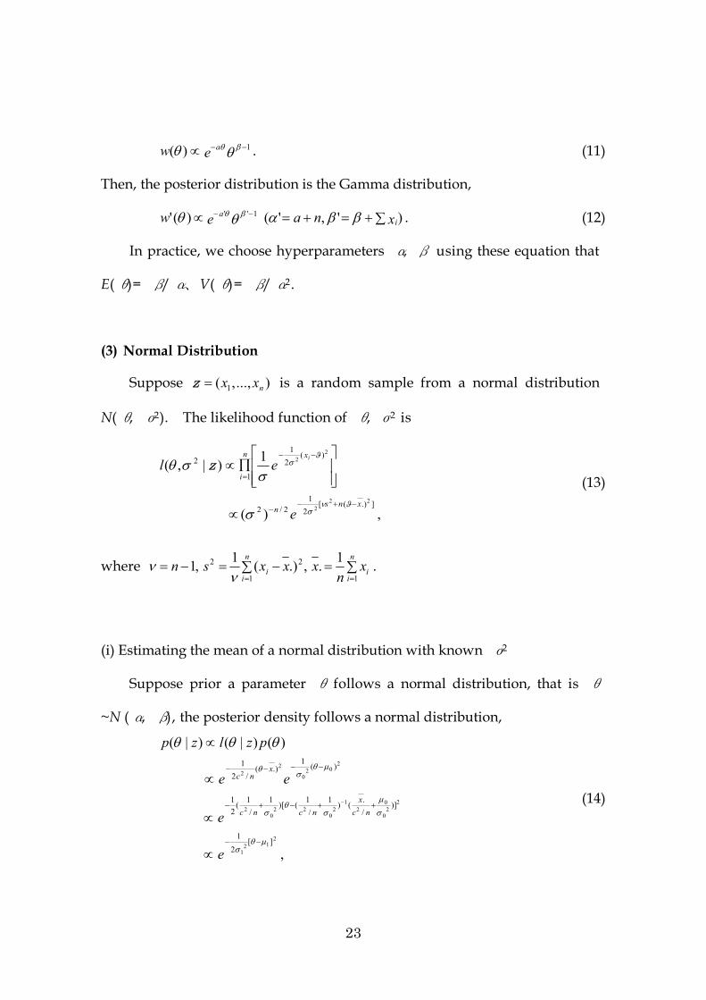
θθ βθ 1)( −−∝ ew a . (11)
Then, the posterior distribution is the Gamma distribution,
∑+=+=∝ −− )','()(' 1'' xnaew ia ββαθθ βθ . (12)
In practice, we choose hyperparameters α, β using these equation that
E(θ)= β/ α、V( θ)= β/ α2.
(3) Normal Distribution
Suppose )...,,( 1 nxx=z is a random sample from a normal distribution
N( θ, σ2). The likelihood function of θ, σ2 is
,)(
1)|,(
]).([21
2/2
)(21
1
2
222
22
xnsn
xn
i
e
eli
−+−−
−−
=
∝
∏∝
ϑνσ
ϑσ
σ
σσθ z
(13)
where ∑=−∑=−===
n
ii
n
ii x
nxxxsn
1
2
1
2 1.,.)(1,1ν
ν .
(i) Estimating the mean of a normal distribution with known σ2
Suppose prior a parameter θ follows a normal distribution, that is θ
~N (α, β), the posterior density follows a normal distribution,
,
)()|()|(
212
1
220
02
120
220
2
202
0
22
][21
)]/.()1
/1()[1
/1(
21
)(1).(
/21
µθσ
σ
µ
σθ
σ
µθσ
θ
θθθ
−−
++−+−
−−−−
∝
∝
∝
∝
−
e
e
ee
pzlzp
ncx
ncnc
xnc
(14)
24
where 20
2
20
02
1 1/1/.
σ
σµ
µ+
+
=
nc
ncx
, 20
2
21 1
1
σ
ο+
=
cn .
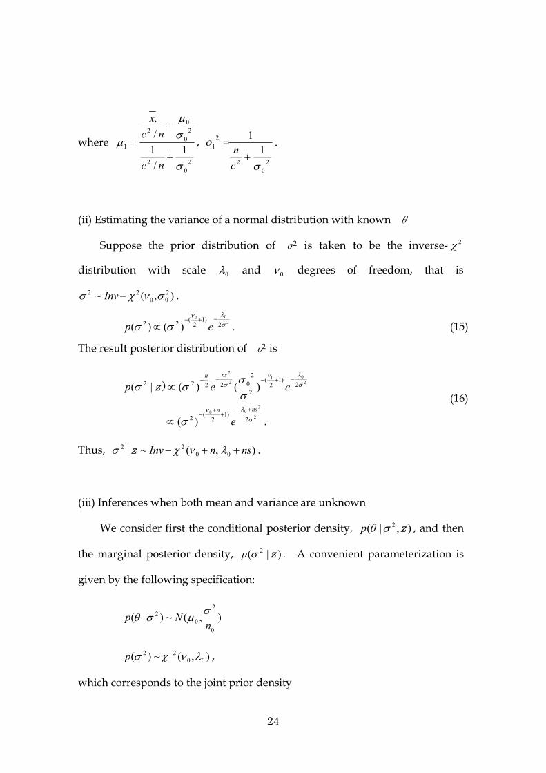
(ii) Estimating the variance of a normal distribution with known θ
Suppose the prior distribution of σ2 is taken to be the inverse- 2χ
distribution with scale 0λ and 0ν degrees of freedom, that is
),(~ 200
22 σνχσ −Inv .
200
2)1
2(22 )()( σ
λν
σσ−+−
∝ ep . (15)
The result posterior distribution of σ2 is
.)(
)()(|(
2
200
200
2
2
2)1
2(2
2)1
2(
2
202222
σλν
σλν
σ
σ
σσ
σσ
nsn
nsn
e
eep
+−+
+−
−+−−−
∝
∝)z (16)
Thus, ),(~| 0022 nsnInv ++− λνχσ z .
(iii) Inferences when both mean and variance are unknown
We consider first the conditional posterior density, ),|( 2 zσθp , and then
the marginal posterior density, )|( 2 zσp . A convenient parameterization is
given by the following specification:
),(~)|(0
2
02
nNp σµσθ
),(~)( 0022 λνχσ −p ,
which corresponds to the joint prior density
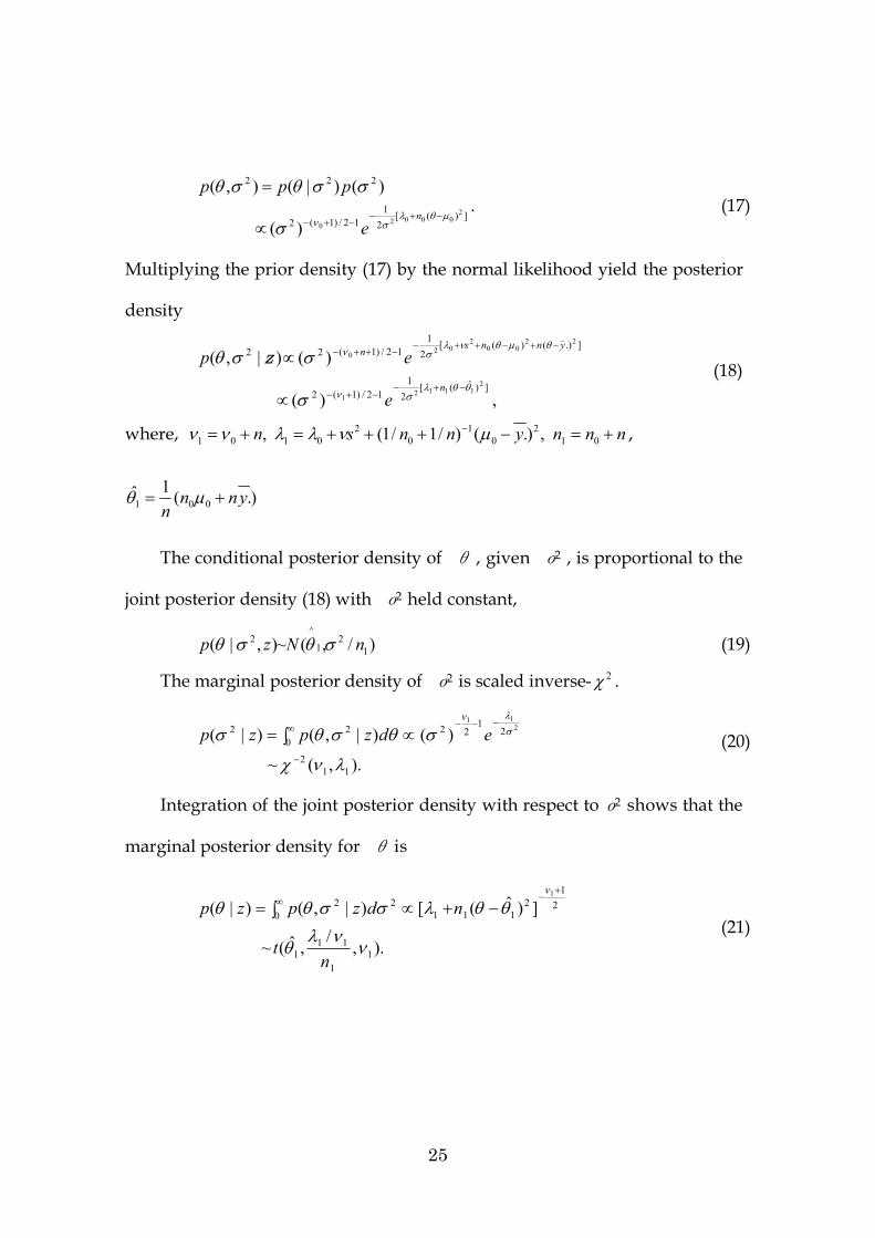
25
])([21
12/)1(2
222
200020)(
)()|(),(µθλ
σνσ
σσθσθ−+−
−+−∝
=
ne
ppp. (17)
Multiplying the prior density (17) by the normal likelihood yield the posterior
density
,)(
)()|,(])ˆ([
21
12/)1(2
].)()([21
12/)1(22
21112
1
2200
2020
θθλσν
θµθνλσν
σ
σσθ−+−
−+−
−+−++−−++−
∝
∝
n
ynnsn
e
ep z (18)
where, nnnynnsn +=−+++=+= −01
20
10
20101 ,).()/1/1(, µνλλνν ,
).(1ˆ001 ynn
n+= µθ
The conditional posterior density of θ , given σ2 , is proportional to the
joint posterior density (18) with σ2 held constant,
)/,(~),|( 12
1
^2 nNzp σθσθ (19)
The marginal posterior density of σ2 is scaled inverse- 2χ .
).,(~
)()|,()|(
112
21
220
22 211
λνχ
σθσθσ σλν
−
−−−∞ ∝∫= edzpzp (20)
Integration of the joint posterior density with respect to σ2 shows that the
marginal posterior density for θ is
).,/
,ˆ(~
])ˆ([)|,()|(
11
111
21
2111
20
21
ννλ
θ
θθλσσθθν
nt
ndzpzp+
−∞ −+∝∫= (21)
26
3.3. Advantages of Bayesian Inference
(1) Practical Use Both Data and Non-Data Information
By applying Bayesian inference, we can use both data as likelihood, and
non-data information as prior distribution. The problems of statistical
measurement approach are resolved in some extent.
We can take indicators that may be predictive of the risk of future losses
into consideration. Such indictors, often referred to as key risk indicators or
early warning indicators, are forward-looking and could reflect potential
sources of operational risk such as rapid growth, the introduction of new
products, employee turnover, transaction breaks, system downtime, etc.
Also, qualitative data, such as self-assessment scoring result can be used
for measuring. This approach affords business line managers incentives to
their risk management through self-assessment process. Consider a situation
where huge operational losses occur in a business line. The maximum
amount of operational risk, or economic capital charge, allotted to that line
becomes so large that line managers might have little incentive to improve
their risk management. In utilizing self-assessment results through Bayesian
inference, increasing levels of sophistication of risk management should
generally be rewarded with a reduction in the operational risk capital
requirement.
27
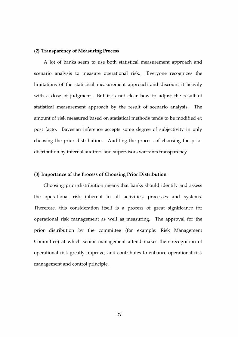
(2) Transparency of Measuring Process
A lot of banks seem to use both statistical measurement approach and
scenario analysis to measure operational risk. Everyone recognizes the
limitations of the statistical measurement approach and discount it heavily
with a dose of judgment. But it is not clear how to adjust the result of
statistical measurement approach by the result of scenario analysis. The
amount of risk measured based on statistical methods tends to be modified ex
post facto. Bayesian inference accepts some degree of subjectivity in only
choosing the prior distribution. Auditing the process of choosing the prior
distribution by internal auditors and supervisors warrants transparency.
(3) Importance of the Process of Choosing Prior Distribution
Choosing prior distribution means that banks should identify and assess
the operational risk inherent in all activities, processes and systems.
Therefore, this consideration itself is a process of great significance for
operational risk management as well as measuring. The approval for the
prior distribution by the committee (for example: Risk Management
Committee) at which senior management attend makes their recognition of
operational risk greatly improve, and contributes to enhance operational risk
management and control principle.

28
4. Examples of Application of Business Practices
4.1. Operations Error Rate
The operations error rate is the main indicator not only to plan various
policies of operations management but also to choose the prior distribution of
the number of operations loss events described in Section 4.2.
We assume that the operations error rate follows Bernoulli trials with
parameter θ. The likelihood of Bernoulli trials follows binominal distribution,
so natural conjugate prior distribution is beta distribution.
In order to know the current operations error rate, it seems adequate to
use the results of recent audit by internal auditors. and not historical data.
But internal audit can’t cover all transactions, has to draw sampling inspection.
For example, internal auditors found an error from 100 samples, is the current
operations error rate 1%? Is the rate 0% because auditors found no error?
We may felt that something was wrong with the results. Accordingly,
Bayesian inference appears.
Based on the results of audits until now and statistics about operations,
with taking expected number of transaction and clerks, procedures of risk
management, skills and morals of clerks into consideration, we choose the
prior distribution for θ. In choosing, descriptive statistics of beta
distribution such as mean, mode, median and variance are used. Multiplied
the prior distribution by likelihood obtained from the latest result of audits, we
29
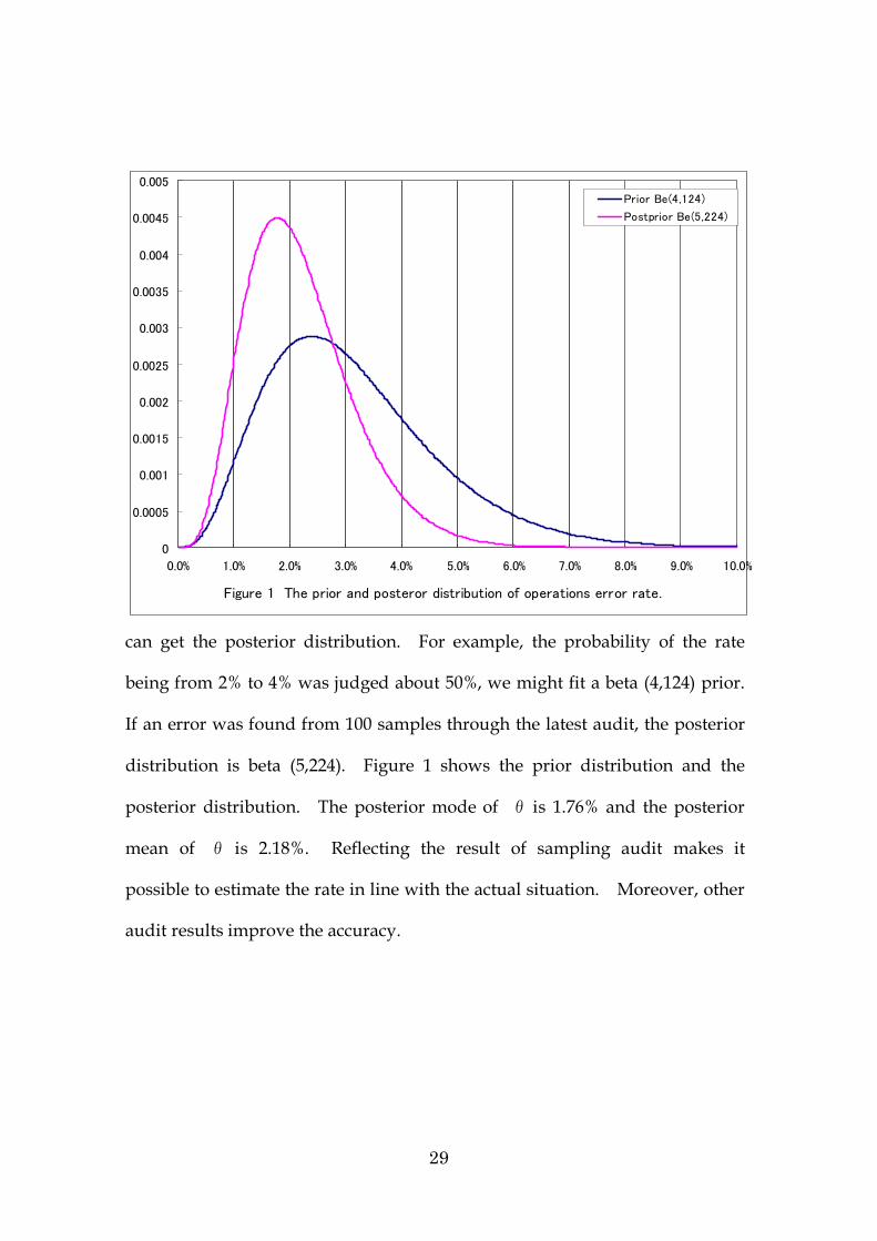
can get the posterior distribution. For example, the probability of the rate
being from 2% to 4% was judged about 50%, we might fit a beta (4,124) prior.
If an error was found from 100 samples through the latest audit, the posterior
distribution is beta (5,224). Figure 1 shows the prior distribution and the
posterior distribution. The posterior mode of θ is 1.76% and the posterior
mean of θ is 2.18%. Reflecting the result of sampling audit makes it
possible to estimate the rate in line with the actual situation. Moreover, other
audit results improve the accuracy.
Figure 1 The prior and posteror distribution of operations error rate.
0
0.0005
0.001
0.0015
0.002
0.0025
0.003
0.0035
0.004
0.0045
0.005
0.0% 1.0% 2.0% 3.0% 4.0% 5.0% 6.0% 7.0% 8.0% 9.0% 10.0%
Prior Be(4,124)
Postprior Be(5,224)
30
4.2. Number of Operations Loss Events
Operations loss event is resulting from manifestation of operations risk
defined as the possibility of losses arising from negligent administration by
employees, accidents, or unauthorized activities. It is natural that, even if
operations loss rate is constant, as transaction volume increases, the number of
operations loss events increases, because the number of operations loss events
= transaction volume × operations loss event rate. The number of
operations loss events per a year has only one or two digits, in contrast that
transaction volume is at least ten millions. Therefore, operations loss event
rate is microscopic; to estimate the rate within an acceptance error range is
very difficult. So, we fit an appropriate distribution to the number of events
itself in order to estimation. The applications of Bayesian inference can reflect
the trend of transaction volume.
Because operations loss event rate is microscopic, we apply Poisson
distribution. Natural conjugate prior distribution is gamma distribution.
Based on historical data, after considering the factors such as external
circumstance, the situation of other banks, the trend of operations error rate
mentioned above, transaction volume, their risk management system, and so
on, we choose the prior distribution of the number of operations loss event rate
θ. The quality factors like professional moral of employee influence so much
that we should take into account. Then, multiplying the recent data of
operations loss events as likelihood decides the posterior distribution.
31
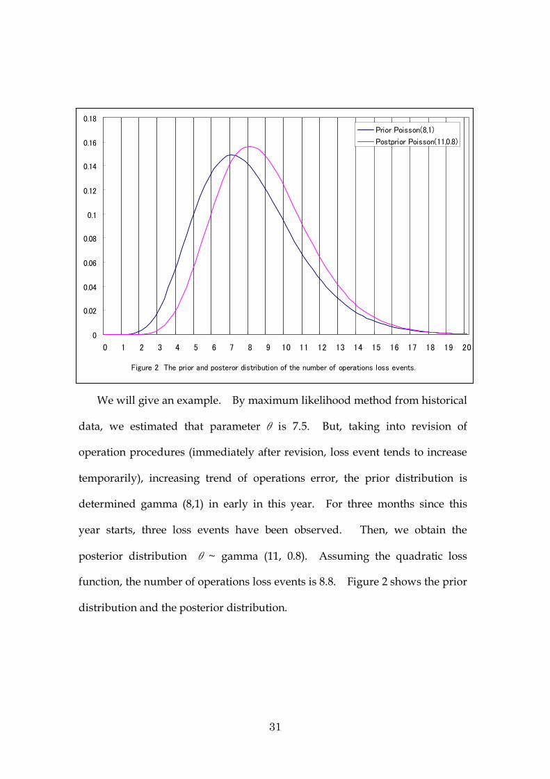
We will give an example. By maximum likelihood method from historical
data, we estimated that parameter θ is 7.5. But, taking into revision of
operation procedures (immediately after revision, loss event tends to increase
temporarily), increasing trend of operations error, the prior distribution is
determined gamma (8,1) in early in this year. For three months since this
year starts, three loss events have been observed. Then, we obtain the
posterior distribution θ ~ gamma (11, 0.8). Assuming the quadratic loss
function, the number of operations loss events is 8.8. Figure 2 shows the prior
distribution and the posterior distribution.
Figure 2 The prior and posteror distribution of the number of operations loss events.
0
0.02
0.04
0.06
0.08
0.1
0.12
0.14
0.16
0.18
0 1 2 3 4 5 6 7 8 9 10 11 12 13 14 15 16 17 18 19 20
Prior Poisson(8,1)
Postprior Poisson(11,0.8)

32
4.3. Severity of Operations Loss Event
The method for application to severity of operations loss event is same.
The distributions of parameters only differ. Supposed the severity X follows
lognormal distribution. For example, by maximum likelihood method from
historical 31 data, we estimated logX~N(15.2, 1.3). Taking an enormous loss
event occurred at other bank, the trend of increasing amount per a transaction,
and so on, we choose the prior distribution p(θ| σ2)~N(16, σ2/31)、 p( σ2)~
χ- 2(30,48). About three loss events occurred for three months since this year
starts, log-mean is 15.67 and log-variance is 2.06. Finally, we obtain the
posterior distribution p( θ|z)~ t(15.98, 0.04, 33)、p( σ2|z)~ χ-2(33, 52.3).
Assuming the quadratic loss function, the severity of operations loss events
follows logX~N(15.98, 1.68). Expectation of X is ¥20,175,912.
33
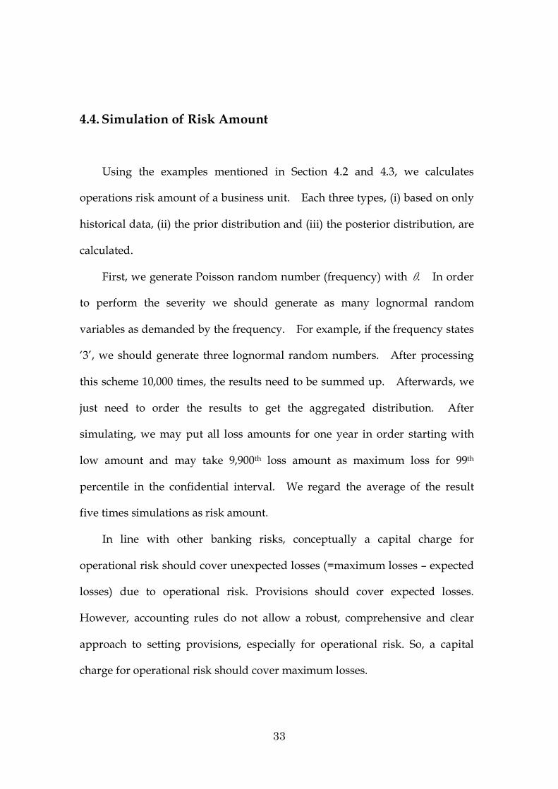
4.4. Simulation of Risk Amount
Using the examples mentioned in Section 4.2 and 4.3, we calculates
operations risk amount of a business unit. Each three types, (i) based on only
historical data, (ii) the prior distribution and (iii) the posterior distribution, are
calculated.
First, we generate Poisson random number (frequency) with θ. In order
to perform the severity we should generate as many lognormal random
variables as demanded by the frequency. For example, if the frequency states
‘3’, we should generate three lognormal random numbers. After processing
this scheme 10,000 times, the results need to be summed up. Afterwards, we
just need to order the results to get the aggregated distribution. After
simulating, we may put all loss amounts for one year in order starting with
low amount and may take 9,900th loss amount as maximum loss for 99th
percentile in the confidential interval. We regard the average of the result
five times simulations as risk amount.
In line with other banking risks, conceptually a capital charge for
operational risk should cover unexpected losses (=maximum losses – expected
losses) due to operational risk. Provisions should cover expected losses.
However, accounting rules do not allow a robust, comprehensive and clear
approach to setting provisions, especially for operational risk. So, a capital
charge for operational risk should cover maximum losses.
34
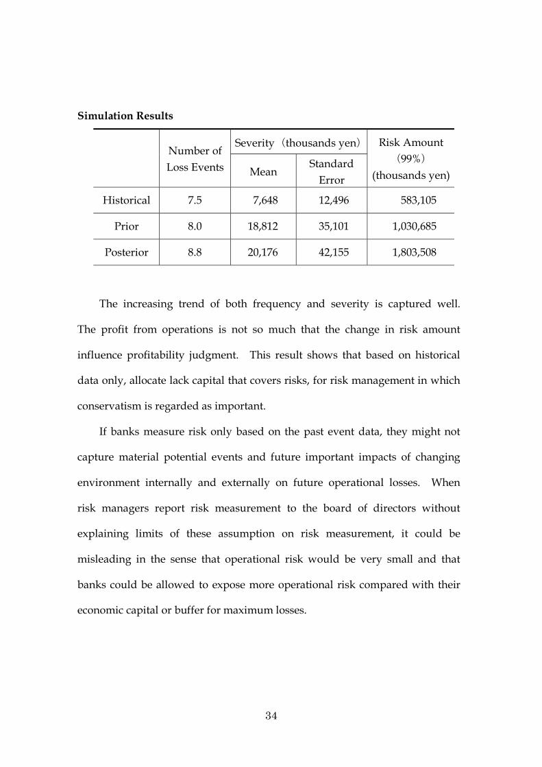
Simulation Results
Severity(thousands yen) Number of Loss Events Mean
Standard Error
Risk Amount (99%)
(thousands yen)
Historical 7.5 7,648 12,496 583,105
Prior 8.0 18,812 35,101 1,030,685
Posterior 8.8 20,176 42,155 1,803,508
The increasing trend of both frequency and severity is captured well.
The profit from operations is not so much that the change in risk amount
influence profitability judgment. This result shows that based on historical
data only, allocate lack capital that covers risks, for risk management in which
conservatism is regarded as important.
If banks measure risk only based on the past event data, they might not
capture material potential events and future important impacts of changing
environment internally and externally on future operational losses. When
risk managers report risk measurement to the board of directors without
explaining limits of these assumption on risk measurement, it could be
misleading in the sense that operational risk would be very small and that
banks could be allowed to expose more operational risk compared with their
economic capital or buffer for maximum losses.

35
4.5. Profitability Judgment
This example is about entry or exit of subsidiaries. Suppose a bank
established a subsidiary given operations by other companies including banks
last year. From the first, the items on business plan were based on
supposition. Needless to say, the capital allocated by the parent company,
covering the subsidiary’s risk, was determined without historical data.
In first year, only a loss event with small amount was occurred. Under
drawing up next year’s plan, can the parent company allocate the subsidiary
capital based only results last year? Is there no danger of underestimation?
We should apply Bayesian Inference.
If the results like observed in first year continue for several years, the
posterior distribution update by the excellent result, risk capital requirement
will decrease.
Parent company judge profitability of the subsidiary based on not
after-tax profit itself but the one after deducting cost of capital. Even if
after-tax profit is in the black, when the profit after deducting cost of capital
goes into red, the parent company makes exacting demands to the subsidiary.
In case of the bad future prospect, the parent company may decide to dissolve
the subsidiary. Risk amount influences seriously profit judgment in the form
of cost of capital.
36
5. Discussion
Bayesian inference is very powerful tool for measuring operational risk,
but there are a number of outstanding issues to be resolved. We are going to
examine the following issues.
(1) Choosing Prior Distribution
The prior distributions represent a description of opinion and knowledge
about the parameters of a certain distribution. In the prior resides most of the
criticism of Bayesian Inference, and we must be very reasonable in choosing
one prior over another. In choosing the prior distribution, which factors must
be taken into account? We should research the methods for translating
qualitative assessments such as scorecards into quantitative metric. It is
important to establish quantitative data such as self-assessment scoring or
results objectively.
So called ‘elicited prior’ is basically the subjective opinion of the value of
parameters before any data is available (or if only limited data is available).
At the current stage in Operation Research, few measurement software
packages are available, but those using Bayesian inference use subjective
opinion to evaluate the parameters. Suppose that several experts are asked to
fill in their opinions about the quantiles of a certain kind of operational event
in a business unit. Given the results, we can fit a prior distribution based on
the elicited opinion from experts.
37
If the approach proposed in this paper spreads among bank industries, via
supervisions, there is a fair possibility that the factors to be considered will be
found.
(2) Validation
Anyway, the first thing we have to do is to put high priorities on
collecting robust loss database. Banks must begin to systematically track
relevant operational risk data by business line across the firm. The ability to
monitor loss events and effectively gather loss data is a basic step for
operational risk.
Further work is needed by both banks and supervisors to develop a better
understanding of the key assumptions of measuring techniques, the necessary
data requirements, the robustness of estimation techniques and appropriate
validation methods (e.g. goodness-of-fit tests of the distribution types and
interval estimation of the parameters) that could be used by banks and
supervisors.
38
References:
Basel Committee on Banking Supervision (1998) ‘’Framework for Internal
Control Systems in Banking Organizations”.
Basel Committee on Banking Supervision (1998) “Operational Risk
Management”.
Basel Committee on Banking Supervision (2001) “The New Basel Capital
Accord, Second Consultative Package”.
Basel Committee on Banking Supervision (2001) “Working Paper on the
Regulatory Treatment of Operational Risk”.
Basel Committee on Banking Supervision (2001) “Sound Practice for the
Management and Supervision of Operational Risk”.
Basel Committee on Banking Supervision (2001) “Internal Audit in Banks
and the Supervisor’s Relationship with Auditors”.
Basel Committee on Banking Supervision (2002) “The Quantitative Impact
Study for Operational Risk: Overview of Individual Loss Data and
Lessons Learned”.
Cruz, M. G. (2002) Modeling, Measuring and Hedging Operational Risk,
London: Wiley.
Frachot, A., George, P. and Roncalli, T. (2001) “Loss Distribution Approach
for Operational Risk”, Working Paper.
Gelman, A., Carlin, J. B., Stern, H. S. and Rubin, D. B. (1995) Bayesian Data
Analysis, CHAPMAN & HALL.
39
Hiwatashi, J. and Ashida H. (2002) ‘’Advancing Operational Risk Management
Using Japanese Banking Experiences’’, Bank of Japan, Audit Office
Working Paper No.00-1, February.
Jorion, P. (2001) Value at Risk: The New Benchmark for Managing Financial
Risk, McGraw-Hill.
Klugman, S. A., Panjer, H. H. and Willmot, G. E. (1998) Loss Models: from
Data to Decisions, John Wiley & Sons.
Kotz, S. and Nadarajah, S. (2000) Extreme Value Distributions: Theory and
Applications’, Imperial College Press, London.
Marshall, C. (2001) Measuring and Managing Operational Risks in Financial
Institutions: Tools, Techniques and Other Resources, John Wiley & Sons.
Mori, T., Hiwatashi, J., and Ide, K. (2000) ‘’Measuring Operational Risk in
Japanese Major banks’’, Bank of Japan, Financial and Payment System
Office Working Paper No.00-1, July.
Mori, T., Hiwatashi, J., and Ide, K. (2000) ‘’Challenges and Possible Solutions
in Enhancing Operational Risk Measurement’’, Bank of Japan, Financial
and Payment System Office Working Paper No.00-3, September.
Mori, T., and Harada, E. (2001) ‘’Internal Measurement Approach to
Operational Risk Capital Charge’’, Bank of Japan, Financial and Payment
System Office Working Paper No.01-2, March.
Matsubara, N. (1979) Ishikettei no Kiso, Asakura Shoten.
Press, S. J. (1989) Bayesian Statistics: Principles, Models, and Applications.
New York: Wiley.
40
Smith, R. (2000) ‘’Bayesian Risk Analysis’’, in Extremes and Integrated Risk
Management, P. Embrechts (ed.), Risk Publications, London, Chapter 17,
pp.235-252.
Shigemasu, T. (1985) Bayes Tokei Nyuumon, Tokyo Daigaku Shuppan
Suzuki, Y. (1978) Toukei Kaiseki, Chikuma Shobou.
Winkler, R. L. (1972) Introduction to Bayesian Inference, Holt, Reinehalt &
Winston, Inc.
Watanabe, H. (1999) Bayes Tokeigaku Nuumon, Fukumura Shuppan.
Recommended