Announcements
Office hours this week Tuesday 3.30-5 (as usual) and Wednesday 10.30-12
HW6 posted, due Monday 10/20

CS 188: Artificial Intelligence
Bayes Nets: Exact Inference
Instructor: Stuart Russell--- University of California, Berkeley

Bayes Nets
Part I: Representation
Part II: Exact inference
Enumeration (always exponential complexity)
Variable elimination (worst-case exponential complexity, often better)
Inference is NP-hard in general
Part III: Approximate Inference
Later: Learning Bayes nets from data

Examples: Posterior marginal probability
P(Q|e1,..,ek) E.g., what disease might I have?
Most likely explanation: argmaxq,r,s P(Q=q,R=r,S=s|e1,..,ek) E.g., what did he say?
Inference
Inference: calculating some useful quantity from a probability model (joint probability distribution)

Inference by Enumeration in Bayes Net
Reminder of inference by enumeration: Any probability of interest can be computed by summing
entries from the joint distribution Entries from the joint distribution can be obtained from a BN
by multiplying the corresponding conditional probabilities P(B | j, m) = α P(B, j, m) = α e,a P(B, e, a, j, m) = α e,a P(B) P(e) P(a|B,e) P(j|a) P(m|a) So inference in Bayes nets means computing sums of
products of numbers: sounds easy!! Problem: sums of exponentially many products!
B E
A
MJ

6
Can we do better?
Consider uwy + uwz + uxy + uxz + vwy + vwz + vxy +vxz 16 multiplies, 7 adds Lots of repeated subexpressions!
Rewrite as (u+v)(w+x)(y+z) 2 multiplies, 3 adds
e,a P(B) P(e) P(a|B,e) P(j|a) P(m|a) = P(B)P(e)P(a|B,e)P(j|a)P(m|a) + P(B)P(e)P(a|B,e)P(j|a)P(m|a) + P(B)P(e)P(a|B,e)P(j|a)P(m|a) + P(B)P(e)P(a|B,e)P(j|a)P(m|a)
Lots of repeated subexpressions!
7
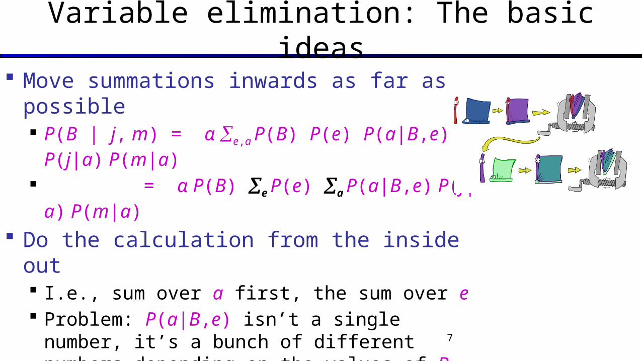
Variable elimination: The basic ideas Move summations inwards as far as possible
P(B | j, m) = α e,a P(B) P(e) P(a|B,e) P(j|a) P(m|a) = α P(B) e P(e) a P(a|B,e) P(j|a) P(m|a)
Do the calculation from the inside out I.e., sum over a first, the sum over e Problem: P(a|B,e) isn’t a single number, it’s a bunch of
different numbers depending on the values of B and e Solution: use arrays of numbers (of various dimensions)
with appropriate operations on them; these are called factors

Factor Zoo

Factor Zoo I
Joint distribution: P(X,Y) Entries P(x,y) for all x, y |X|x|Y| matrix Sums to 1
Projected joint: P(x,Y) A slice of the joint distribution Entries P(x,y) for one x, all y |Y|-element vector Sums to P(x)
A \ J true false
true 0.09 0.01
false 0.045 0.855
P(A,J)
P(a,J)
Number of variables (capitals) = dimensionality of the table
A \ J true false
true 0.09 0.01

Factor Zoo II
Single conditional: P(Y | x) Entries P(y | x) for fixed x, all y Sums to 1
Family of conditionals: P(X |Y) Multiple conditionals Entries P(x | y) for all x, y Sums to |Y|
A \ J true false
true 0.9 0.1
P(J|a)
A \ J true false
true 0.9 0.1
false 0.05 0.95
P(J|A)
} - P(J|a)
} - P(J|a)

Operation 1: Pointwise product
First basic operation: pointwise product of factors (similar to a database join, not matrix multiply!) New factor has union of variables of the two original factors Each entry is the product of the corresponding entries from
the original factors
Example: P(J|A) x P(A) = P(A,J)
P(J|A)P(A)
P(A,J)A \ J true false
true 0.09 0.01
false 0.045 0.855
A \ J true false
true 0.9 0.1
false 0.05 0.95
true 0.1
false 0.9 x =
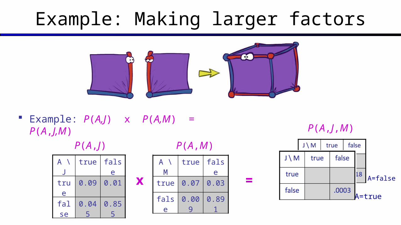
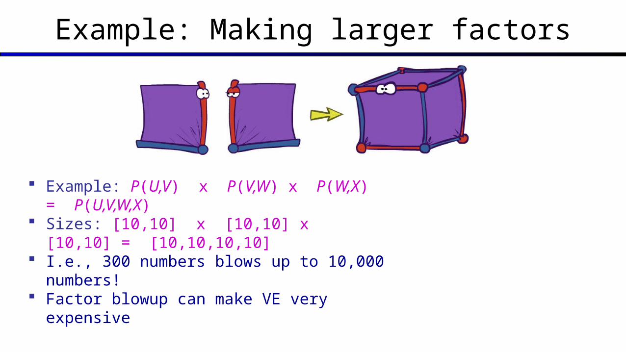
Example: Making larger factors
Example: P(A,J) x P(A,M) = P(A,J,M)
P(A,J)A \ J true false
true 0.09 0.01
false 0.045 0.855x =
P(A,M)A \ M true false
true 0.07 0.03
false 0.009 0.891A=true
A=false
P(A,J,M)
Example: Making larger factors
Example: P(U,V) x P(V,W) x P(W,X) = P(U,V,W,X) Sizes: [10,10] x [10,10] x [10,10] = [10,10,10,10] I.e., 300 numbers blows up to 10,000 numbers! Factor blowup can make VE very expensive

Operation 2: Summing out a variable
Second basic operation: summing out (or eliminating) a variable from a factor Shrinks a factor to a smaller one
Example: j P(A,J) = P(A,j) + P(A,j) = P(A)
A \ J true false
true 0.09 0.01
false 0.045 0.855
true 0.1
false 0.9
P(A)P(A,J)
Sum out J

Summing out from a product of factors
Project the factors each way first, then sum the products Example: a P(a|B,e) x P(j|a) x P(m|a) = P(a|B,e) x P(j|a) x P(m|a) + P(a|B,e) x P(j|a) x P(m|a)

Variable Elimination

Variable Elimination
Query:
Start with initial factors: Local CPTs (but instantiated by evidence)
While there are still hidden variables (not Q or evidence): Pick a hidden variable H Join all factors mentioning H Eliminate (sum out) H
Join all remaining factors and normalize

18
Variable Elimination
function VariableElimination(Q , e, bn) returns a distribution over Qfactors ← [ ]for each var in ORDER(bn.vars) do factors ← [MAKE-FACTOR(var, e)|factors] if var is a hidden variable then factors ← SUM-OUT(var,factors) return NORMALIZE(POINTWISE-PRODUCT(factors))
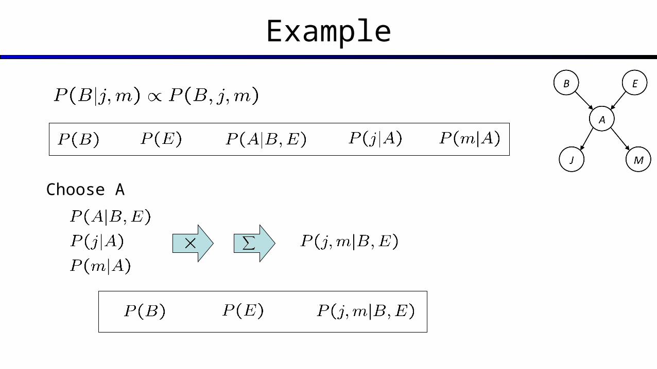
Example
Choose A

Example
Choose E
Finish with B
Normalize
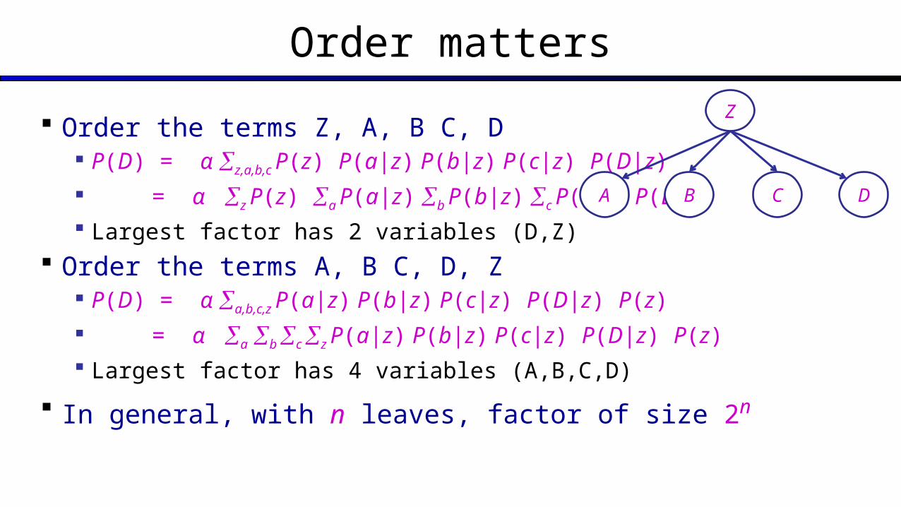
Order matters
Order the terms Z, A, B C, D P(D) = α z,a,b,c P(z) P(a|z) P(b|z) P(c|z) P(D|z) = α z P(z) a P(a|z) b P(b|z) c P(c|z) P(D|z) Largest factor has 2 variables (D,Z)
Order the terms A, B C, D, Z P(D) = α a,b,c,z P(a|z) P(b|z) P(c|z) P(D|z) P(z) = α a b c z P(a|z) P(b|z) P(c|z) P(D|z) P(z) Largest factor has 4 variables (A,B,C,D)
In general, with n leaves, factor of size 2n
D
Z
A B C

VE: Computational and Space Complexity
The computational and space complexity of variable elimination is determined by the largest factor (and it’s space that kills you)
The elimination ordering can greatly affect the size of the largest factor. E.g., previous slide’s example 2n vs. 2
Does there always exist an ordering that only results in small factors? No!

Worst Case Complexity? Reduction from SAT
CNF clauses:1. A v B v C2. C v D v A3. B v C v D
P(AND) > 0 iff clauses are satisfiable => NP-hard
P(AND) = S.0.5n where S is the number of satisfying assignments for clauses => #P-hard

Polytrees
A polytree is a directed graph with no undirected cycles
For poly-trees the complexity of variable elimination is linear in the network size if you eliminate from the leave towards the roots This is essentially the same theorem as for tree-
structured CSPs

Bayes Nets
Part I: Representation
Part II: Exact inference
Enumeration (always exponential complexity)
Variable elimination (worst-case exponential complexity, often better)
Inference is NP-hard in general
Part III: Approximate Inference
Later: Learning Bayes nets from data
Recommended