Econometric Model of the U.S. Sheep Industry for Policy Analysis
Luis A. Ribera, David P. Anderson, and James W. Richardson Agricultural & Food Policy Center
Department of Agricultural Economics Texas A&M University
TAMU 2124 College Station, TX 77843-2124
Phone: (979) 845-7042 e-mail: [email protected]
Selected Paper prepared for presentation at the American Agricultural Economics Association Annual Meeting, Denver, Colorado, July 1-4, 2004
Copyright 2004 by [Luis A. Ribera, David P. Anderson, and James W. Richardson]. All rights reserved. Readers may make verbatim copies of this document for non-commercial purposes by any means, provided that this copyright notice appears on all such copies.

1
INTRODUCTION Sheep were first domesticated in Central Asia about 10,000 years ago (Ensminger
and Parker). Their use then was the same as today, to provide two products, meat and
wool. Today, sheep production has evolved to include more than 200 breeds worldwide.
In the U.S. two areas dominate sheep production, the range state region and the
farm flock region (Anderson, 1994). The range state region includes the 16 Western
states and Texas. Commercial production in these states is made up of large
concentrations of sheep grazing large areas of the range. In 2002, these states accounted
for about 85 percent of the total U.S. sheep flock. The farm flock region includes the rest
of the U.S. and accounts for the remaining 15 percent. These flocks generally use more
meat-oriented breeds than wool producing breeds (USDA Sheep and Goats).
The U.S. sheep industry is small compared to the rest of the world. In 2002, it
accounted for 0.67 percent of the world’s sheep inventory with 4.91 million head and
about 1.42 percent of the world’s wool production with about 41 million pounds of clean
fleece (USDA Cotton and Wool Outlook). China is the world’s largest sheep producer
with 135 million head (in 2002), followed closely by Australia with 119 million head
and, in smaller scale, New Zealand, Argentina, Uruguay, and South Africa. In the world’s
wool production, Australia is the largest producer with 946 million pounds of clean fleece
(in 2002), followed by New Zealand, China, Argentina, Uruguay and South Africa.
Australia is the world’s largest exporter of wool with 406 million pounds of clean fleece
followed by New Zealand, Argentina, Uruguay and South Africa. The U.S. is the 8th
largest importer of wool with 75 million clean pounds (USDA Cotton and Wool
Outlook).
2
Besides being a small producer of sheep internationally, the U.S. sheep industry
has been declining for many years. From 1940 to 2002, the number of stock sheep has
declined significantly, from 49 million head in 1942 to 4.1 million head in 2002 (USDA
Agricultural Statistics).
Many factors have contributed to the decline of the sheep industry. The per capita
consumption of lamb and mutton has fallen from 2.9 pounds in 1970 to 1.2 pounds in
2002 (USDA Livestock, Dairy and Poultry Outlook). During the same period of time,
per capita consumption of poultry increased from 34.1 pounds to 93.1 pounds. Two other
major factors contributing to the reduction in the U.S. sheep industry are: scarcity of
labor and predator losses (Stillman, et al., 1990). Moreover, the growth of manmade
fiber is another major factor for this downward trend
In an effort to slow the rate of decline in the U.S. sheep industry, the U.S.
Congress passed the Wool Act of 1954. Under the Wool Act, incentive payments were
made to producers to encourage wool production (Anderson, 1994). However, in 1993,
Congress passed a three-year phase out of the Wool Act incentive payments with the last
payments occurring in 1996 (Anderson, 2001). Since that program phase out, a series of
ad hoc programs have been passed to support the industry due to a series of setbacks,
caused in large part, by events beyond industry control such as strong U.S. dollar which
encouraged an increase in imports, and financial difficulties for domestic mills. The
2002 Farm Bill reinstated support for the industry by implementing a marketing loan
program, similar to other commodities, with loan rates of $0.40 and $1.00 per pound for
un-graded and graded wool, respectively (USDA Cotton and Wool Outlook).

3
The livestock industry has a large body of research studies in agricultural
economics. However, few studies have been performed on the sheep industry, either in
the U.S. or the rest of the world. Some of the studies reviewed are: Debertin, et al.
(1983) developed a monthly econometric model for the U.S. sheep industry with
particular emphasis on the changes in the industry that have taken place during 1964
to1980. Whipple and Menkaus (1989) developed a dynamic supply model of the U.S.
sheep industry. Whipple and Menkaus (1990a) estimated a price dependent farm,
wholesale, and retail demand for lamb. Anderson (1994) estimated a supply and demand
model of the U.S. sheep and mohair industry for policy analysis using annual data from
1973 to 1992.
The objective of this research is to analyze the impacts of different levels of loan
rates on the U.S. sheep industry. Two different levels of loan rates will be analyzed: free
market (zero loan rate), and an increase of 100 percent ($2.00 /lb) of the actual loan rate.
The results of this research will be useful to sheep producers, as well as other
stakeholders in the U.S. industry. By analyzing and providing information on the impacts
of alternative polices, the industry will be better able to address the impacts of policy
alternatives and craft policies to address emerging issues.
In addition, imports and exports of sheep products play a major role in the U.S.
sheep industry. Therefore, the econometric sector model developed for this study will
concentrate on developing a robust trade component to analyze their effects on U.S. trade
with the 7 leading international producers and consumers of sheep: Australia, United
Kingdom, South Africa, Argentina, and New Zealand, Canada, and Mexico. Canada and

4
Mexico, while being smaller markets, are the main recipients of the U.S. lamb and live
sheep exports.
MATERIALS AND METHODS
The review of past literature provides important information on how to develop an
econometric model of the sheep industry. The conceptual model used in this study builds
on the work done by Anderson (1994) and to some extent the studies by Debertin, et al.
(1983), and Whipple and Menkhaus (1989 and 1990a). A major expansion to previous
studies is that 7 different regions or countries will be modeled in order to better estimate
the impacts of exchange rates on trade.
Data
Annual data will be used to construct the models for the U.S. sheep industry.
Table 1 contains the data and abbreviations used for all the equations included in the
model development and estimation. The data was collected from the U.S. Department of
Agriculture, the Livestock Marketing information Center, Food and Agricultural
Organization (FAO) and International Monetary Fund (IMF). Since the sheep industry
have been declining for roughly the past 50 years, a time trend will have a large impact in
the model. Therefore, following Anderson’s (1994) approach, shortening the data period
to the last 22 years (1980-2002) will show the different structure of the industries while
allowing an adequate number of degrees of freedom.
Model Development
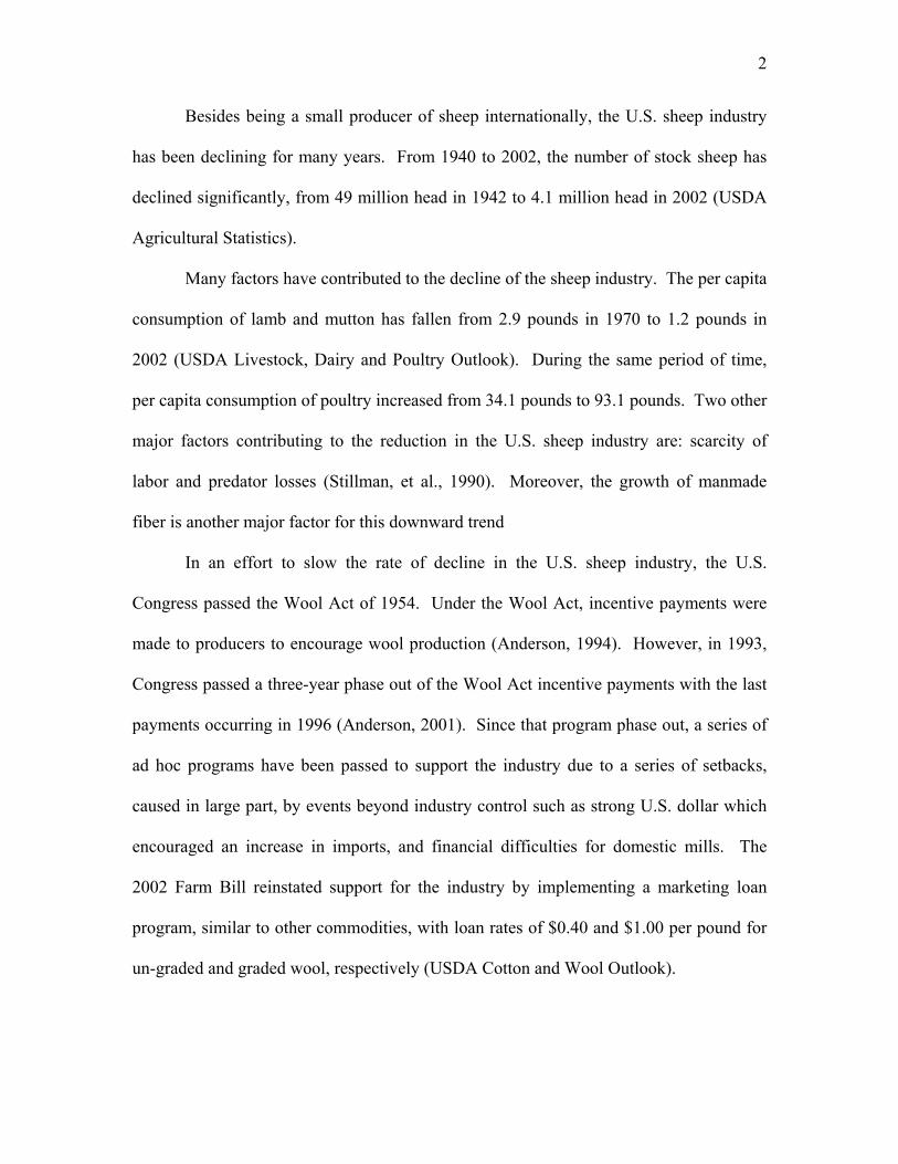
Figure 1 shows a flow chart of the U.S. sheep industry. The number of stock
sheep (ewes) represents stock breeding ewes in the herd. Ewes are the starting point of
the sheep industry and all the other variables will revolve around it. The number of

5
Table 1. Variables for the sheep industry model
Data Variable Name Data Variable Name
Ewes SEWE Income INC Lamb Crop LCROP Population POP Replacements EWEL Beef Price BP Rams & Wethers RAMS Pork Price PP Death Loss SDIE & LDIE Chicken Price CP Ewe Slaughter SSLTR Incentive Price INCPR Lamb Slaughter LSLTR Lamb Consumption LAMBCONS Carcass Weight DWT Wool Exports WEXP Wool Production WOOLPROD Wool Imports WIMP Fleece Weight FLEECE U.S. Mill Use WMILL Dressed Weight WEIGHT Wool Stocks WSTK Lamb Price LAMBPR Palmer Drought Index PDI Sheep Price EWEPR Feed Concentrate Cost FEED Wool Price WOOLPR Australia Lamb Production AUSL Wool Incentive Price WSPTR Nez Zealand Lamb Production NZL Mexico Domestic Demand MEXDD South Africa Wool Prodcution SAW Mexico Exchange Rate MEXEXCH United Kingdom Wool Production UKW Australia Exchange Rate AUSEXCH Argentina Wool Production ARGW Canada Exchange Rate CANEXCH Polyster Price POLYPR Australian Wool Production AUSW Cotton Price COTPR New Zealand Wool Production NZW Acrylic Price ACRPR Live Sheep Export SHPEXP Live Sheep Import SHPIMP Canada Sheep Production CANPRD
stock sheep is reduced by death loss, slaughter, and lamb crop. Replacements and
imports increase the number of ewes. Ewe and lamb slaughter, along with lamb and
mutton imports make up the total domestic meat production. Total sheep numbers times
wool yield gives the total wool production and adding the wool imports gives the total
wool use.
The models for the sheep industry will use single econometric equations and
biological identities. As mentioned above, data from 7 different countries will be
included to provide estimates of the impacts of exchange rates on imports and exports.
The 7 different countries will be Australia, United Kingdom, South Africa,
6
Figure 1. Flow Chart of the U.S. Sheep Industry Model
Slaughter
Death Loss Stock Sheep
(Ewes)
Lamb Crop
Slaughter
Total Domestic Meat Production
Lamb & Mutton Imports
Domestic Meat Demand
U.S. Sheep Numbers
U.S. Wool Yield
U.S. Wool Production
U.S. Wool Use
Wool Imports
Death Loss
Kept for Replacement
Sheep, Lamb and Mutton Production &Demand from:
• Australia • New Zealand • Mexico • Canada • ROW
Meat Exports
U.S. Price
World Price
Wool Exports
U.S. Price
World Price
Wool Production & Demand from:
• Australia • New Zealand • United Kingdom • South Africa • Argentina

7
New Zealand, Argentina, Canada, and Mexico. Three stage least squares (3SLS) will be
the estimation procedure. The model will be validated through historical simulation. The
equations used for this study are presented in Table 2.
Equation 1 is an identity and it represents the herd inventory. The number of
breeding ewes is equal to the number of breeding ewes in the last period minus death
loss, slaughter and exports, plus imports and replacement.
Equation 2 represents the death loss of ewes and is a function of number of
breeding ewes, Palmer Drought Index (PDI), price of lamb, sheep and wool, and time.
Historical weighted PDIs for the months of June, July, and August were used as a proxy
of drought ranging from 2.88, mild to moderate wetness, to –3.41, severe drought. PDI is
hypothesized to have a negative effect to death loss ewes, as well as prices. Ewe
slaughter (3) is a function of number of ewes, and prices of lamb, sheep and wool.
Higher sheep prices will increase the number of ewe slaughtered, while higher prices for
lamb and wool are hypothesized to have a negative effect since producers try to build up
the herd to increase lamb and wool production.
The number of live sheep exported (4) is assumed to be a function of number of
ewes, prices, and Mexican exchange rate ($Mex/1$US) since most of the live sheep are
exported to Mexico. Lower lamb, sheep and wool prices will encourage herd liquidation,
and exports. A strong dollar is hypothesized to reduce export levels. Live sheep imports
(5) is a function of Canadian sheep production since Canada is the main exporter to the
U.S. in live sheep, exchange rate ($Can/1$US), and lamb and sheep prices. Higher
Canada sheep production and/or higher lamb and sheep prices is hypothesized to increase
live sheep imports. A strong U.S. dollar is expected to increase U.S. import levels.

8
Table 2. Equations and identities for sheep industry model.
. 1. Ewest = Ewest-1 – Death Losst-1 – Slaughtert-1 – Exportst-1 + Importst-1 + Replacements
2. Ewe Death Losst = f(Ewest, PDIt, Lamb Pricet-1, Sheep Pricet-1, Wool Pricet-1, Timet)
3. Ewe Slaughtert = f(Ewest, Lamb Pricet-1, Sheep Pricet-1, Wool Pricet-1)
4. Exportst (live) = f(Ewest, Lamb Pricet-1, Sheep Pricet-1, Wool Pricet-1, Mexico X-Ratet)
5. Importst (live) = f(Canada Productiont, Canada X-Ratet, Sheep Pricet, Lamb Pricet)
6. Lamb Cropt = f(Ewest, PDIt, Timet)
7. Replacementst = f(Lamb Cropt, Ewest, Lamb Pricet-1, Sheep Pricet-1, Wool Pricet-1)
8. Lamb Deatht = f(Lamb Cropt, PDIt, Timet)
9. Lamb Slaughtert = f(Lamb Cropt, Ewest, Lamb Pricet-1, Sheep Pricet-1, Wool Pricet-1, Sub Pricet-1)
10. Lamb Productiont (meat) = Lamb Slaughtert * Carcass Weightt
11. Carcass Weightt = f(Timet, Lamb Pricet-1, Feed Concentrate Costt-1))
12. Total Raw Wool Prodt = Total Sheept * Fleece Yieldt
13. Fleece Yieldt = f(Timet, PDIt, Wool Pricet-1, Lamb Pricet-1, Fleece Yieldt-1)
14. Lamb Importst (meat) = f(Australia Prodt, New Zealand Prodt, Lamb Pricet, Australia X-Ratet)
15. Wool Importst (raw) = f(Big 5 Wool Productiont, Wool Pricet, Australia X-Ratet)
16. Lamb Domestic Demandt = f(Lamb Pricet, Incomet, Sub Pricet, timet)
17. Lamb Exportst = f(Lamb Pricet, Mexico X-Ratet, Mexico Domestic Demandt)
18. Wool Demandt = f(Wool Pricet, Incomet, Cotton Pricet, Polyester Pricet, Acrylic Pricet)
19. Wool Exportst = f(Wool Pricet, Australia X-Ratet)
20. Wool Stockst = f(Wool Pricet, Incomet, Big 5 Wool Productiont) .
PDI = Palmer Drought Index Sub Price = Beef Price, Pork Price, and Chicken Price Big 5 = Australia, United Kingdom, South Africa, New Zealand, and Argentina
Lamb crop (6) is a function of ewes, PDI and time. Drought is hypothesized to
lower lamb crop and time is set to capture any change in technology. Lamb crop has
three possible destinations: ewe replacement, lamb death, and lamb slaughter. Ewe
replacement (7) is a function of lamb crop, number of ewes, and prices. Higher prices of
lamb and wool are hypothesized to have a positive effect on replacement numbers, while
higher sheep prices should have a negative impact. Death loss of lamb (8) is a function

9
of lamb crop, PDI and time. Lamb slaughter (9) is assumed to be a function of lamb
crop, number of ewes, and prices of lamb sheep and wool, as well as prices of beef, pork
and chicken, lagged one period. Higher lamb prices are hypothesized to have a positive
effect on the number of lamb slaughtered.
Total domestic lamb production (10) is an identity and is calculated as total lamb
slaughtered times its carcass weight. Carcass weight (11) is hypothesized to be a
function of time, lamb price, and feed concentrate cost. Feed concentrate cost is the cost
of feed too finish the lambs that are going to be slaughtered and is expected to have a
negative relationship with carcass weight. Total raw wool production (12) is an identity
calculated as the total number of sheep times the estimated fleece weight per sheep.
Fleece yield (13) is modeled as a function of PDI, time, wool and lamb prices, and itself
lagged one period.
Lamb imports (14) are modeled as a function of lamb price, Australia exchange
rate ($Aus/1$US), and Australia and New Zealand production. A strong dollar and/or
higher lamb production by Australia and New Zealand is hypothesized to increase
imports. Wool imports (15) are a function of wool production of the Big 5 (Australia,
United Kingdom, South Africa, New Zealand, and Argentina), wool price, and Australia
exchange rate.
Domestic demand for lamb (16) is assumed to be a function of lamb, beef, pork
and chicken prices and Income. Economic theory tells us that as the price of lamb
increases, its demand will decrease and as the price of substitutes, beef, pork and chicken,
increase the demand for lamb will increase. Lamb exports (17) are a function of lamb
price and Mexican domestic demand and exchange rate.
10
Wool demand (18) is a function of wool price, income, and cotton, polyester and
acrylic prices. Income is hypothesized to have a positive effect on demand because wool
is expected to be a normal or luxury good. Wool exports (19) are a function of wool
price and exchange rate and wool stocks (20) are set to be a function of wool price,
income, world stocks and wool production by the Big5.
Solving Supply and Demand
The supply and selected demand system will be solved simultaneously to
determine the market-clearing price. It involves iterating on the price that equates the
supply and demand model. The market clearing equation is:
Supply – Demand = 0
The estimated parameters will be used with the EViews© “Solver” routine to solve this
nonlinear optimization. The routine then solves the equation, supply – demand = 0, and
yields the market, or equation solving, price. Industry parameters and price will be
projected as a baseline to compare policy alternatives.
RESULTS AND DISCUSSION
The econometric estimation results for each equation are presented in Table 3.
Each equation was evaluated for goodness-of-fit during the estimation process. Adjusted
R2 statistics and p-values were the primary measure of goodness-of-fit. Variables, based
upon economic theory, were retained if they were statistically significant at least at the 95
percent confidence level.
Lamb crop (LCROP) was estimated as a function of number of stock ewes, DPI
and trend. All variables were statistically significant at the 99 percent confidence level as
shown by their p-values lower than 0.01 and the adjusted R2 is very high, 0.9841. As

11
expected, the number of ewes was the most important determinant of the size of lamb
crop. PDI was also important in the lamb crop equation, but yielded the opposite sign.
We would expected a positive relationship between lamb crop and PDI since as PDI goes
up means that the level of drought was reduced
Replacement numbers (EWEL) yielded a high adjusted R2 (0.9825). Number of
stock ewes yielded a positive sign, as expected, because some ewes must be replaced
each year due to age or usefulness. However, the sign for lamb crop and sheep price are
contrary to expectations. As lamb crop and sheep price increases we would expect an
increase in the number of replacement in order to build the herd.
Sheep death loss (SDIE) was estimated as a function of number of stock ewes, PDI, lamb
price, sheep price and trend. All variables are statistically significant and the model
yielded a high adjusted R2, 0.9257. All variables have the expected signs except for lamb
price that have the opposite sign. Lamb death loss (LDIE) is a function of PDI and trend.
Both variables are statistically significant and yielded a low adjusted R2, 0.6548.
However, PDI has an opposite sign than expected.
Lamb slaughter (LSLTR) estimated results show that all variables in the equation
are statistically significant at least at the 95 percent level and all signs agree with
economic theory. Sheep prices lagged (EWEPRt-1) has a negative sign since the producer
will want to reduce slaughter increase the herd size. Beef price lagged (BPt-1) also has a
negative relationship as expected since beef is considered substitute for lamb. The
dummy variable D01 accounts for the years that the wool subsidies were terminated in
1996 and reinstated in 2002.

12
Table 3. Regression equations for sheep industry model estimated over 1980-2002 .
Adjusted R2
LCROPt = 2443.6 + 0.56963(SEWEt) – 31.6940(PDIt) –36.2685(TIME) 0.9841 (0.000) (0.016) (0.002) EWELt = -679.7 + 0.3648(SEWEt) – 0.1804(LCROPt) – 7.47(EWEPRt) 0.9825 (0.000) (0.000) (0.000) SDIEt = 0.0682(SEWEt) – 6.6147(PDIt) + 2.5217(LAMBPRt-1) – 4.408(EWEPRt-1) – 4.8104(TIMEt) 0.9257 (0.000) (0.0210) (0.000) (0.000) (0.000) LDIEt = - 40.755(TIMEt) + 94.651(PDIt) 0.6548
(0.000) (0.0495) LSLTRt = 2068.2 + 0.628(LCROPt) – 24.61(EWEPRt-1) – 7.418(BPt)– 258.172(D01) 0.9604 (0.000) (0.000) (0.000) (0.014) (0.000) SSLTRt = 176.56 + 0.0398(SEWEt) – 4.5538(EWEPRt) + 25.182(WOOLPRt) 0.9049 (0.000) (0.000) (0.000) (0.004) DWTt = 43.8157 + 0.0437(LAMBPRt-1) + 4.4409(TIME)2 0.9147
(0.000) (0.004) (0.000) FLEECEt = 1.89 + 0.7418(FLEECEt-1) + 0.1018(WOOLPRt-1) – 0.0226(PDIt) 0.7880 (2.84) (1.56) (1.70) SHPEXTt = 7.5031(MEXDDt) – 0.3066(D01) 0.2552 (0.000) (0.000) SHPIMPt = - 235.417 + 6.9208(CANPRDt) + 0.5898(LAMBPRt) + 51.871(CANEXCHt) 0.6294 (0.000) (0.000) (0.000) (0.002) LMIMPt = -39.05 + 0.236(AUSLt) - 10.59(NZL) + 57.7(AUSEXCHt) + 19.2166(D01) 0.8283 (0.001) (0.000) (0.020) (0.000) LMEXPt = 12.4042 – 0.1107(LAMBPRt) + 0.0384(MEXDDt) 0.7670 (0.001) (0.000) (0.050) WMILLt = – 0.006(WOOLPRt) + 65.3(COTPRt) - 269.6(POLYPRt) + 60.82(INCPRt) 0.6879 (0.008) (0.000) (0.000) (0.025) WIMPt = 0.782(NZWt) +0.512(UKWt) + 27.456(WOOLPRt) - 44.15(INCPRt) + 65.048(D01) 0.7993 (0.000) (0.000) (0.000) (0.000) (0.000) LAMBCONSt = 312.7 – 0.019(LAMBPRt) + 0.007(INCt) – 6.168(TIMEt) + 0.26(LAMBCONSt-1) 0.6686 (0.000) (0.000) (0.020) (0.000) (0.000) WEXPt = 23.451 – 1.7952(WOOLPRt) + 6.2215(INCPRt) – 13.626(D01) 0.6484 (0.000) (0.021) (0.000) (0.000) .
Variables are defined in Table 1. Values in parenthesis are p-values

13
Sheep slaughter (SSLTR) estimated results shows that all variables in the
equation are statistically significant at least at the 0.01 level and all signs agree with
economic theory except for wool price. As wool price increases we would expect sheep
slaughter to decrease since they will be kept to produce more wool.
The dress weight (DWT) equation showed that both explanatory variables are
significant at least at the 0.01 level and their signs agree with expectations, i.e. a higher
lamb price is expected to yield a higher dress weight. Fleece weight (FLEECE)
estimated parameters agree with economic theory, except for PDI, and it also has a low
adjusted R2, 0.7880.
Live sheep exports (SHPEXT) equation was a function of Mexico domestic
demand and the dummy variable (D01). Mexico is the major importer of U.S. sheep.
This equation performed very poorly adjusted R2, 0.2552, although many different
variables were used to estimate this equation. Live sheep imports (SHPEXP) yielded also
a low adjusted R2, 0.6294, however, all variables have the expected signs. Canada sheep
production has a positive impact on live sheep imports since Canada is the main exporter
of live sheep to the U.S. Moreover, Canada exchange rate has a positive effect on live
sheep imports since a strong U.S. dollar makes foreign goods relatively cheaper.
Lamb imports (LMIMP) were modeled as a function of Australia and New
Zealand lamb production, Australia exchange rate and the dummy D01. The variables
are significant at the 99 percent level and the signs agree with economic theory, except
for New Zealand lamb production. As Australia and New Zealand lamb production
increases, more lamb is imported, however, there is a negative relationship with New
Zealand. The effect of the exchange is as expected since a strong U.S. dollar increases
14
imports. Lamb exports (LMEXP) was estimated as a function of lamb price and Mexico
domestic demand and all variables were significant at the 95 percent level. In addition,
both variables comply with economic theory since as lamb price increases less lamb will
be exported, and as Mexico’s domestic demand increases, lamb exports increase.
Wool imports (WIMP) was estimated as a function of New Zealand and United
Kingdom wool production, price of wool, wool incentive payment and D01. The signs of
all the variables were as expected. Positive relationship between wool price, New
Zealand and UK wool production on wool imports, and negative relationship with
incentive payments.
U.S. mill demand for wool (WMILL) was estimated as a function of wool price,
cotton and polyester price, and wool incentive payments. This equation gave an adjusted
R2 of 0.6878 and all of its variables were significant at the 95 percent level. All variables
comply with economic theory except for cotton price, which has a positive relationship
with mill demand for wool. On the other hand, polyester price have a negative
relationship with wool mill demand, as well as wool price. Wool incentive payments
have a positive relationship with mill demand for wool since an increase of wool
incentive payment will increase supply of wool and consequently lower the price of wool.
Wool export (WEXP) was modeled as a function of wool price, incentive wool
price and the dummy D01. This equations yielded a low adjusted R2 0.6484, but all of is
explanatory variables were significant at least at the 95 percent level and comply with
economic theory. As wool price increases, wool exports decrease. Also as wool
incentive payments increase, wool exports increases.

15
Finally, lamb consumption (LAMBCONS) was modeled as a function of price of
lamb, income, trend and lamb consumption lagged one period. All variables were
statistically significant at the 95 percent level and their signs agree with economic theory.
Lamb price (LAMBPR) has a negative sign meaning that as price of lamb increases, lamb
consumption decreases. Moreover, income has a positive sign, which agrees with
economic theory for normal or luxury goods.
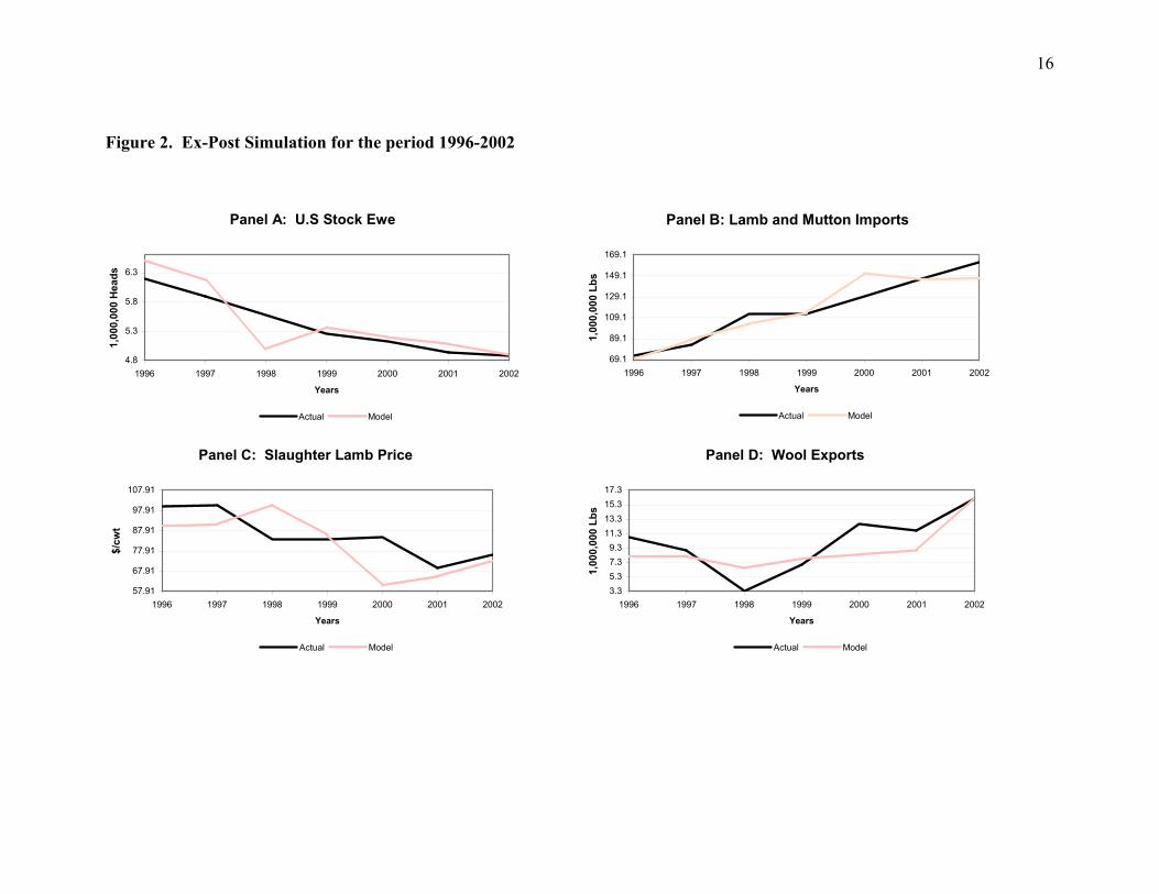
Ex-Post Simulation
The model was simulated in EViews© using the “model solver” routine for the
1996-2002 time period and results are presented in Figure 2. Figure 2A contains the
actual and simulated stock ewe numbers generated by the model. The model simulates
the historical data fairly well, following the trend, but slightly overestimating the ewe
numbers all the periods except in 1998 where the simulated model drops sharply below
the historical data. The model simulates lamb and mutton imports very well
overestimating imports in 1997 and 2000, and underestimating imports in 1998 and 2000
(Figure 2B). Figure 2C shows the actual and ex post simulation of slaughter lamb price.
The simulated model seems to move opposite to the historical values. However, for 2001
and 2002 the model follow the movements of the historical lamb prices very well.
Finally, simulated and actual wool exports values are shown in Figure 2D. Again
the simulated model seems to move in opposite directions than the actual data, but follow
the movements of the actual data for the last couple of years. Moreover, it fails to
capture the magnitude of the drastic decrease on wool exports in 1998. In general, the
model seem to not follow the actual data in the early years, but tends to recover in the
16
Figure 2. Ex-Post Simulation for the period 1996-2002
Panel A: U.S Stock Ewe
4.8
5.3
5.8
6.3
1996 1997 1998 1999 2000 2001 2002
Years
1,00
0,00
0 H
eads
Actual Model
Panel B: Lamb and Mutton Imports
69.1
89.1
109.1
129.1
149.1
169.1
1996 1997 1998 1999 2000 2001 2002
Years
1,00
0,00
0 Lb
s
Actual Model
Panel C: Slaughter Lamb Price
57.91
67.91
77.91
87.91
97.91
107.91
1996 1997 1998 1999 2000 2001 2002
Years
$/cw
t
Actual Model
Panel D: Wool Exports
3.35.37.39.3
11.313.315.317.3
1996 1997 1998 1999 2000 2001 2002
Years
1,00
0,00
0 Lb
s
Actual Model

17
last couple of years of the ex post simulation except for the lamb and mutton imports.
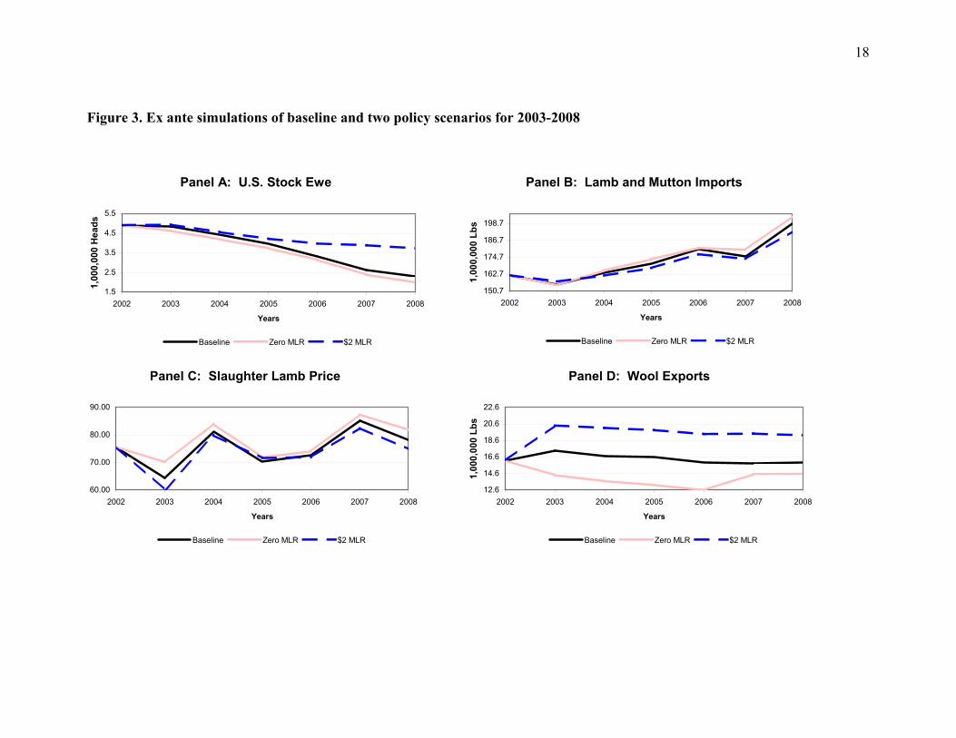
Baseline Analysis (Preliminary Results)
An ex-ante simulation was performed to develop a baseline projection for the
2003-2008 time horizon. The baseline assumptions included:
• No change in the loan rate set at $1 per pound of wool
• Exogenous variables projections were available from the FAPRI January 2004
Baseline and also forecasted using ARIMA and VAR models.
The baseline simulation for stock ewe numbers continue to decline during the entire time
horizon reaching about 2.5 million head by 2008 (Figure 3A). Imports of lamb and
mutton were projected to increase to about 200 million pounds by 2008 (Figure 3B).
Slaughter lamb prices move up and down during the whole time horizon, but a slightly
positive trend can be seen (Figure 3C). Finally, wool exports are projected to increase by
about 1.2 million pounds in 2003, but tend to decline thereafter (Figure 3D).
Policy Alternative (Preliminary Results)
The policy alternative analyzed in this study is two levels of wool marketing loan
rate: scenario 1 has a zero loan rate, while scenario 2 has a loan rate of $2.00 per pound
of wool.
Stock ewe continues its negative trend under both scenarios, but the magnitude of
the negative trend is much smaller for scenario 2 compared to scenario 1 and the baseline
(Figure 3A). Under scenario 1, stock ewe number reaches about 2 million head in 2008
compared to 3.7 million under scenario 2.
Lamb and mutton imports are also affected under the two scenarios (Figure 3B).
The loan rate is hypothesized to have a positive effect on the short run and a negative
18
Figure 3. Ex ante simulations of baseline and two policy scenarios for 2003-2008
Panel A: U.S. Stock Ewe
1.5
2.5
3.5
4.5
5.5
2002 2003 2004 2005 2006 2007 2008
Years
1,00
0,00
0 H
eads
Baseline Zero MLR $2 MLR
Panel B: Lamb and Mutton Imports
150.7
162.7
174.7
186.7
198.7
2002 2003 2004 2005 2006 2007 2008
Years
1,00
0,00
0 Lb
s
Baseline Zero MLR $2 MLR
Panel C: Slaughter Lamb Price
60.00
70.00
80.00
90.00
2002 2003 2004 2005 2006 2007 2008
Years
Baseline Zero MLR $2 MLR
Panel D: Wool Exports
12.6
14.6
16.6
18.6
20.6
22.6
2002 2003 2004 2005 2006 2007 2008
Years
1,00
0,00
0 Lb
s
Baseline Zero MLR $2 MLR
19
effect on the long run on lamb and mutton imports since a higher loan rate will make the
producers increase the replacement number to build the herd. Therefore in the short run,
a higher loan rate will increase the number of lamb and mutton imports. The model
complies with a priori expectations since under scenario 2 (higher loan rate) lamb and
mutton imports increase in 2003 compare to both scenario 1 and baseline. Afterwards, it
falls below both scenario 1 and baseline.
Slaughter lamb price also shows an impact under both scenarios (Figure 3C). A
higher loan rate is expected to increase slaughtering of lamb that will lead to a decrease in
lamb prices, while a lower loan rate will have the opposite effect. Figure 3C shows that
lamb prices under scenario 1 are higher than under scenario 2.
Finally, Figure 3D shows the effect that wool exports have due to the two levels
of loan rates. As expected a higher loan rate will increase wool production that will lead
to and increase in wool exports. The conversely is true for a decrease in loan rate.
SUMMARY AND CONCLUSIONS
The sheep industry has been in a downward trend since the early 1940s.
Therefore, producers and their congressmen have been concerned about the industry’s
survival and programs to aid the industry. Due to the limited number of research studies
on the sheep industry, there is a need to develop an econometric model of both industries
for policy analysis purposes.
The objective of this research is to analyze the impacts of different levels of loan
rates on the U.S. sheep industry. Two different levels of loan rates will be analyzed: free
market (zero loan rate), and an increase of 100 percent ($2.00 /lb) of the actual loan rate.
For this purpose, an ex-ante simulation was performed to develop a baseline projection

20
for the 2003-2008 time horizon and compared to the simulations under the two policy
scenarios. The main assumption of the baseline is that there will be no change in the
actual loan rate set at $1 per pound of wool.
Results of the ex ante simulation show that stock ewe numbers will continue its
decrease under both scenarios, but the rate of decrease will be lower under a higher loan
rate. Under scenario 2, lamb and mutton imports goes from a slightly increase in the first
year to a slightly decrease in the following years compared to the baseline and scenario 1.
Under scenario 1 slaughter lamb prices will increase while wool exports decreases
compared to scenario 2.
Higher marketing loan payment will result in reduced decline in ewe numbers, but
will not reverse their downward trend. Raising the marketing loan rate would likely
increase the U.S. wool exports. On the other hand, removing the current marketing loan
rate will have minimal impact on ewe numbers and raise lamb imports and lamb price
very slightly. Moreover, eliminating the marketing loan rate would reduce wool exports
slightly.
21
REFERENCES
Anderson, D.P. “An Econometric Model of the U.S. Sheep and Mohair Industries for Policy Analysis.” Ph D Dissertation, Texas A&M University, College Station, Texas, 1994.
Anderson, D.P. “Wool and Mohair Policy.” Department of Agricultural Economics,
Texas A&M University. 2001. Anderson, D.P., J.W. Richardson and E.G. Smith. “Evaluating a Marketing Loan
Program for Wool and Mohair.” Agricultural & Food Policy Center, Texas A&M University. February 2001. BP-2001-1.
Chambers, R.G. and R.E. Just. “Effects of Exchange Rate Changes on U.S. Agriculture:
A Dynamic Analysis.” American Journal of Agricultural Economics. 68(1986):55-66.
Debertin, D.L., A.L. Meyer, J.T. Davis, and L.D. Jones. “A Monthly Econometric Model
of the U.S. Sheep Industry.” Department of Agricultural Economics, University of Kentucky. 1983
Ensminger, M.E. and R.O. Parker. Sheep and Goat Science. The Interstate Printers and
Publishers, Danville, IL, 1986. [FAO] Food and Agricultural Organization. FAOSTAT Agricultural Data, September
2003. [FAPRI] Food and Agricultural Policy Research Institute. 2004 U.S. and World
Agricultural Outlook. Staff report [IMF] International Monetary Fund. Country economic profile 2003. [LMIC] Livestock Marketing Information System. Sheep and lamb historical statistics. Meat Facts. The American Meat Institute, Washington, DC. Various Issues. Rayner A.C. “A Model of the New Zealand Sheep Industry.” The Australian Journal of
Agricultural Economics. 12(1968):1-15. Stillman, R., T. Crawford, and L. Aldrich. “The U.S. Sheep Industry.” U.S. Department
of Agriculture, Economic Research Service, Commodity Economics Division. Washington, D.C., 1990.
U.S. Department of Agriculture, Agricultural Stabilization and Conservation Service.
“ASCS Commodity Fact Sheet.” Various Issues. Washington, D.C.
22
U.S. Department of Agriculture, Economic Research Service. “Cotton and Wool Outlook.” Various Issues. Washington D.C.
U.S. Department of Agriculture, Economic Research Service. “Livestock, Dairy, and
Poultry Outlook: Red Meat Yearbook.” Various Issues. Washington D.C. U.S. Department of Agriculture, National Agricultural Statistics Service. “Sheep and
Goats.” Various Issues. Washington D.C. Whipple, G.D. and D.J. Menkhaus. “Supply Response in the U.S. Sheep Industry.”
American Journal of Agricultural Economics. 71(1989):126-135. Whipple, G.D. and D.J. Menkhaus. “Welfare Implication of the Wool Act.” Western
Journal of Agricultural Economics. 15(1990a):33-44. Witherell, W.H. “A Comparison of the Determinants of Wool Production in the Six
Leading Producing Countries: 1949-1965.” American Journal of Agricultural Economics. 51(1969):139-58).
Recommended