INTERNATIONAL JOURNAL ON SMART SENSING AND INTELLIGENT SYSTEMS, VOL. 5, NO. 2, JUNE 2012
487
CONTINUOUS TIME IDENTIFICATION AND
DECENTRALIZED PID CONTROLLER OF AN
AEROTHERMIC PROCESS
M. Ramzi*, H. Youlal** , M. Haloua***
*LASTIMI, Ecole Supérieure de Technologie de salé, Université Mohamed V Agdal, Maroc,
** UFR Automatique et Technologies de l’Information, Faculté des Sciences de Rabat,
Avenue Ibn Batouta, B.P. 1014, Rabat, Maroc *** EMI, Avenue IbnSina, B.P. 765 Agdal Rabat, Maroc
Submitted: Apr. 11, 2012 Accepted: May 9, 2012 Published: June 1, 2012
Abstract- The interactions between input/output in multivariable processes represent a major
challenge in the design of decentralized controllers. In this paper, a simple method for the design of
decentralized PID controller is proposed. It consists to combine the conventional PID controller
with the static decoupler approach. For each single loop, the individual controller is independently
designed by applying the internal model control (IMC) tuning rules. To demonstrate the
effectiveness of the proposed method, the PID controller with and without decoupling is
implemented on an aerothermic process. It is a pilot scale heating and ventilation system equipped
with a heater grid and a centrifugal blower, fully connected through the Humusoft MF624 data
acquisition system for real time control. The outcome of the experimental results is that the main

M. Ramzi and H. Youlal, Continuous Time Identification and Decentralized PID Controller of an Aerothermic Process
488
control objectives, such as set-point tracking and interactions rejection are well achieved. The
experimental results have shown that the proposed method provides a significant improvement
compared to conventional PID controller.
Index terms: Continuous-time identification, aerothermic process, decentralized PID controller, static
decoupling, TITO control systems.
I. INTRODUCTION
The heating and ventilation system plays an important role in many industrial sectors
including chemical, mineral, drying and distillation processes, as well as pharmaceutical and
agro alimentary production units. It is argued that the temperature control is no more a
challenging control problem in most of these applications. Nevertheless, some practical issues
in many temperature control applications stimulate new developments and further
investigations [1-5].
For education and training purposes, many aerothermic processes are available. They
highlight most heating and ventilation problems, and they are widely referenced in the process
control literature. Different prototypes of these processes have been used to check new control
strategies and many results were reported in the single variable control cases [6-10].
As most industrials multivariable processes, the aerothermic processes are generally subject to
significant interactions between its main variables. However, they were not explicitly
considered in most reported control. Worth to mention herein that the basic factory control
system delivered with most of aerothermic processes is restricted to the classical analog PID
controller without taking into account of interactions between its main parameters [11].
In this paper, we highlight further aspects of multi-loops PID controller which consist to
associate this conventional controller with the partial static decoupler approach in order to
eliminate the interactions between the main aerothermic process parameters. In this synthesis,
a multivariable transfer function is identified using the numeric Direct Continuous-Time
Identification (DCTI) approach [12]. This technique has attracted an increasing attention of
several researchers in the last few years [13-18]. It provides a robust and accurate method for
the identification of dynamical systems under the influence of perturbations. Among the
advantages of the DCTI methods, we mention its ability to deal with multi-input multi-output
identification in a straightforward manner from process experimental data and the ease of use
due to the small number of parameters which have to be chosen by the user.
INTERNATIONAL JOURNAL ON SMART SENSING AND INTELLIGENT SYSTEMS, VOL. 5, NO. 2, JUNE 2012
489
The paper content is organized as follows: Section II introduces the description of the
aerothermic process and underlines the interaction between its main variables. Section III
discusses the multivariable continuous-time identification, which represents the first step in
the design of the controllers. The decentralized PID controller is introduced in section IV. Its
parameters are calculated by using the IMC tuning rules. In this section, we recall the main
steps of static decoupler. Section V reports the experimental control results of the aerothermic
process under set-point change of the ventilator speed in order to show its impact on the air
temperature when the PID controller, with and without static decoupler, is applied.
Robustness of the decentralized PID controller is also discussed and a final conclusion is
given.
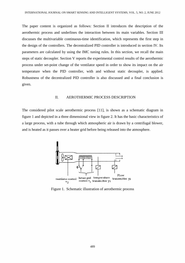
II. AEROTHERMIC PROCESS DESCRIPTION
The considered pilot scale aerothermic process [11], is shown as a schematic diagram in
figure 1 and depicted in a three dimensional view in figure 2. It has the basic characteristics of
a large process, with a tube through which atmospheric air is drawn by a centrifugal blower,
and is heated as it passes over a heater grid before being released into the atmosphere.
Figure 1. Schematic illustration of aerothermic process

M. Ramzi and H. Youlal, Continuous Time Identification and Decentralized PID Controller of an Aerothermic Process
490
Figure 2. Three-dimensional view of aerothermic process
The command objective for the aerothermic process is to regulate the flow and the air
temperature respectively by the PI and PID controllers with and without decoupling the
interaction parameters. The temperature control is achieved by varying the electrical power
supplied to the heater grid. There is an energized electric resistance inside the tube, and due to
the Joule effect, heat is released by the resistance and transmitted, by convection, to the
circulating air, resulting in heated air [6]. The air flow is adjusted by varying the speed of the
ventilator.
This process can be characterized as a non-linear system. The physical principle which
governs the behavior of the aerothermic process is the balance of heat energy. Hence, when
the air temperature and the flow inside the process are assumed to be uniform, a linear system
model can be obtained. This kind of aerothermic process is being used by many researchers to
check their new control strategies [6-10].
As shown in the schematic of the aerothermic process, the system inputs, (u1, u2), are
respectively the power electronic circuit feeding the heating resistance and the ventilator
speed. The outputs, (y1, y2), are respectively the flow and air temperature. The input-output
signals are expressed by a voltage, between 0 and 10 V, issued from the transducers and
conditioning electronics. Figure 3 shows a Two-Input Two-Output (TITO) block diagram of
the aerothermic process.

INTERNATIONAL JOURNAL ON SMART SENSING AND INTELLIGENT SYSTEMS, VOL. 5, NO. 2, JUNE 2012
491
Figure 3: TITO Block diagram
The fundamental relationship between inputs and outputs signal are expressed as:
=
2
1
2221
1211
2
1
U
U
PP
PP
Y
Y (1)
where the P11, P12, P21 and P22 are the continuous process transfer functions which will be
identified in the section III. P12 and P21 are called the process interaction.
To examine the possibility of interaction between the temperature and air flow, two
experiments were carried out. In each case, the two process inputs were held constant and
allowed to settle. If one of them undergoes a step change, the behavior of the other output will
be observed to see if this change had any effect on it. Figure 4 shows the results from both
experiments.
Figure 4. Interactions between the main variables of the aerothermic process

M. Ramzi and H. Youlal, Continuous Time Identification and Decentralized PID Controller of an Aerothermic Process
492
In the first half plot of this figure, the electric voltage supplied to the heater grid is held
constant (at 4V) and the ventilator speed undergoes a step change from 30% to 70% of its full
range. The air temperature varied considerably from 4V (45°C) to 2V (35°C). The second half
plot shows the results when the ventilator speed is held constant and the electric voltage of the
heater grid undergoes a step change, from 40% to 80% of full range. As can be seen, the air
temperature is varied accordingly but the air flow is remained unaffected.
These results show that the air temperature behavior depends also of the operating conditions
of the air flow. Hence, the change in air temperature behavior is provided by two effects: a
direct effect, by the heater grid and indirect effect via the ventilator speed. Our main aim is
then to eliminate the indirect effect.
Equation 2 summarizes this relationship in continuous-time transfer function form.
=
)(
)(
)(0
)()(
)(
)(
2
1
22
1211
2
1
sU
sU
sP
sPsP
sY
sY (2)
Therefore, the figure 3 takes the following new representation:
Figure 5: Partial interaction TITO Block diagram
III. CONTINUOUS-TIME IDENTIFICATION
System identification is an experimental approach to determine the transfer function or
equivalent mathematical description for the dynamic of an industrial process component by
using a suitable input signal. This approach represents the first step in the design of a
controller.
From a conceptual standpoint, the modeling of most mathematical models of industrial
processes is formulated in terms of continuous-time (CT) differential equations using the

INTERNATIONAL JOURNAL ON SMART SENSING AND INTELLIGENT SYSTEMS, VOL. 5, NO. 2, JUNE 2012
493
physicochemical laws. Nonetheless, in the past, the majority of system identification schemes
have been based on discrete-time (DT) models. Their corresponding CT models are obtained
indirectly from the existing DT models.
In fact, the development of CT model identification techniques originated in the last century
[19]. However, it has attracted an increasing attention of several researchers in the recent
years [13-16]. This interest is due to the ability of these approaches to provide consistent
results even for an imperfect noise structure which is the case in most practical applications
[16]. The early contributions on continuous-time identification can be found in [17-18].
For identifying a continuous-time model from discrete sampled data, there exist two main
approaches. The first, namely the indirect approach, it consists to estimate from the sampled
data, an initial DT model and then convert it into a CT model using a standard algorithm for
discrete to continuous-time conversion. The second, namely the direct approach, which
formulates the identification of the CT model directly based on samples of the measured CT
signal. The main computational tools of this approach are based on the Refined Instrumental
Variable method for Continuous-time Systems (RIVC) and its Simplified version (SRIVC)
that are discussed in detail by [20].
In order to generate estimation and validation data for system identification, an experiment is
performed. Data set used for the parameter identification step is build up with Pseudo
Random Binary Sequence (PRBS) signals which are applied simultaneously to the two
manipulated variables of aerothermic process. This data set and their correspondent outputs
are displayed in figure 6. The sampling interval is Ts=1 second. The signals collected, via the
Humusoft MF624 data acquisition module, are yield in the interval (0V, 10V).

M. Ramzi and H. Youlal, Continuous Time Identification and Decentralized PID Controller of an Aerothermic Process
494
Figure 6: Data set for direct continuous-time identification
Based on the outcome analyses of section II, two loops will be considered in the aerothermic
process identification. The first loop will be represented by Two-Inputs (u1, u2) and Single-
Output (y1), TISO. The second loop will be represented by a Single-Input (u2) and a Single-
Output (y2), SISO. After the application of the DCTI approach on first half experimental
sampled data of identification (i.e.: 30 minutes), the identified models of the aerothermic
process suggests that the dynamic relationship between the measured inputs and the measured
outputs for the two loops are linear and first-order plus dead time (FOPDT). The dead time is
equal to 7 seconds for the first loop and is equal to 1 second for the second one. In general,
the transfer function of FOPDT system is given by:
1)(
+=
−
Ts
KesG
Ds
(3)
where K is the steady state gain, D is the dead time, and T is the time constant. The identified transfer functions of the aerothermic process are given by the following system
equation:
=
−
−−
)(
)(
1 + 1.4302s
1.08880
1 + 30.9789s
0.4616-
1 + 34.0716s
0.7891
)(
)(
2
1
77
2
1
sU
sU
e
ee
sY
sY
s
ss
(4)

INTERNATIONAL JOURNAL ON SMART SENSING AND INTELLIGENT SYSTEMS, VOL. 5, NO. 2, JUNE 2012
495
The negative gain in the interactive transfer function implies that the air temperature behaves
in the opposite way. In fact, the interaction effect tends to reduce the air temperature when the
flow increases.
To evaluate the quality of the estimated transfer function models, a cross-validation procedure
has been applied to the remaining experimental data were not used to build the model. Cross-
validation result is plotted in Figures 7. From this figure, it may be observed that there is a
relatively good agreement between the measured and the simulated model output.
To confirm this validation, a numeric test is also applied to evaluate the models quality. It
consists to use the coefficient of determination, given in equation 5, in order to determine the
strength of the linear association between the simulated and measured output.
)var(
)ˆvar(1
y
yyCD
−−= (5)
Table 1 summarizes the results of the coefficient of determination for DCTI approaches.
Table1: Coefficient of Determination
Coefficient of Determination
TISO 0.9914
SISO 0.9920
Figure 7: Cross-validation results (black: measured output; blue: simulated output)

M. Ramzi and H. Youlal, Continuous Time Identification and Decentralized PID Controller of an Aerothermic Process
496
As shown in both figure 7 and table 1, it appears a good similarity between the true system
output and the identified one. Furthermore, the identified process has no modes associated
with eigenvalues in the unstable region.
IV. DECENTRALIZED PID CONTROLLER
a. Decoupling control systems
As shown in section III, changes in second loop might cause an undesirable disturbance in
first loop and hence cause y1 to vary from its desired value. Therefore, the interaction caused
by the second loop needs to be completely or partially eliminated. To do it, the aerothermic
process must be decoupled into separate loops.
There exist two ways to see if a system can be decoupled. The first One is with mathematical
models and the other is a more intuitive educated guessing method. The mathematical
methods include the relative gain array (RGA) method, the Niederlinski Index (NI) and
singular value decomposition (SVD) [21]. In this paper the SVD method is used to discuss the
determination of whether the TITO control scheme can be decoupled to SISO ones. It starts
with the steady state gain matrix of the process as shown in the following equation.
=
)0(0
)0()0(
22
1211
P
PPP (6)
Using P, the calculation of the eigenvalues can be calculated by hand from the following
equations [22]:
2
4)( 222
11
cdbdbs
+−++==β (7)
22
22
22s
cbds
−==β (8)
where b = P112(0)+ P12
2(0); c= P122(0) P22
2(0) and d = P222(0). s1 and s2 are the positive
square roots of the respective eigenvalues. The condition number (CN) is defined as the ratio
of the larger si to the smaller sj:
>=
>=
121
2
212
1
ssifs
sCN
ssifs
sCN
(9)
The greater the CN value, the harder it is for the system in question to be decoupled. A rule of
thumb is that when CN ≥50 the system is nearly singular and decoupling is not feasible [23].
INTERNATIONAL JOURNAL ON SMART SENSING AND INTELLIGENT SYSTEMS, VOL. 5, NO. 2, JUNE 2012
497
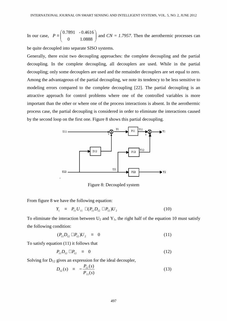
In our case,
=
1.08880
0.4616-0.7891P and CN = 1.7957. Then the aerothermic processes can
be quite decoupled into separate SISO systems.
Generally, there exist two decoupling approaches: the complete decoupling and the partial
decoupling. In the complete decoupling, all decouplers are used. While in the partial
decoupling; only some decouplers are used and the remainder decouplers are set equal to zero.
Among the advantageous of the partial decoupling, we note its tendency to be less sensitive to
modeling errors compared to the complete decoupling [22]. The partial decoupling is an
attractive approach for control problems where one of the controlled variables is more
important than the other or where one of the process interactions is absent. In the aerothermic
process case, the partial decoupling is considered in order to eliminate the interactions caused
by the second loop on the first one. Figure 8 shows this partial decoupling.
.
Figure 8: Decoupled system
From figure 8 we have the following equation:
212121111111 )( UPDPUPY ++= (10)
To eliminate the interaction between U2 and Y1, the right half of the equation 10 must satisfy
the following condition:
0)( 2121211 =+ UPDP (11)
To satisfy equation (11) it follows that
0121211 =+ PDP (12)
Solving for D12 gives an expression for the ideal decoupler,
)(
)()(
11
1212 sP
sPsD −= (13)

M. Ramzi and H. Youlal, Continuous Time Identification and Decentralized PID Controller of an Aerothermic Process
498
b. multivariable decentralized PID controller
In principle, decoupling control can provide two important points. In the first one, the control
loop interactions will be eliminated. Consequently, the stability of the closed-loops system
will be determined only by the stability characteristics of the individual feedback control
loops. In the second one, if the set-point of a controlled variable is changed, it will not have an
effect on the other controlled variables.
Several control approaches such as neural networks, model predictive control can resolve the
multivariable control problems with or without severe interactions. However, these controls
are used primarily on a higher level. In the lower level, improving the performance and
robustness of a system can be made by the improvements in the separate proportional-
differential-integral (PID) loops [24]. In this paper, the improvement is obtained by using the
partial static decoupling where the design is based on the steady state process interactions.
The design equations for the decoupler can be adjusted by setting (s = 0), i.e. the process
transfer functions are simply replaced by their corresponding steady state gains. Hence, the
expression for the ideal decoupler given by the equation 12 becomes:
0.5850)0(
)0(
11
1212 =−=
P
PD (14)
Figure 9 shows the partial decoupling control system for the aerothermic process.
Figure 9: A partial decoupling control system
The PI controller is used to regulate the air flow since this loop has generally very fast
dynamics and its measurement is inherently noisy; while, the air temperature is regulated by
the PID controller. Once a partial decoupler is obtained, the PI and the PID controllers are
designed separately for the two loops. Hence, as shown in figure 9, three controllers are used:
two conventional feedback controllers, PID and PI, plus one decoupler, D12. The input-signal
INTERNATIONAL JOURNAL ON SMART SENSING AND INTELLIGENT SYSTEMS, VOL. 5, NO. 2, JUNE 2012
499
to D12 decoupler, which is designed to compensate the undesirable process interactions, is the
output signal from the feedback PI controller.
The continuous PID controller transfer function can be written as
dt
tdeKdtteKteKtu dip
)()()()( ++= ∫ (15)
where u(t) is the manipulated variable, e(t) the error signal, Kp, Ti, and Td represent
proportional gain, integral gain and derivative gain respectively.
In the Laplace domain, this control equation can be written as:
)()()( sEsKs
KKsU d
ip ++= (16)
To calculate the PI and PID parameters, the Internal Model Control (IMC) tuning rules is
adopted [25]. It is used most frequently in industrial processes because of its many
advantages, including simplicity, robust performance, and its analytical form which is easier
to implement in real time.
The PID controller parameters are given as follows:
)(2
)(
1
)(2
2
β
β
β
+=
+=
++=
DK
TDK
DKK
DK
DTK
d
i
p
(17)
where K represents the steady-state gain, T is the time constant, and D is the time delay of the
system. β should satisfy β > 0.2T and β > 0.25L [26].
V. EXPERIMENTAL RESULTS
To illustrate the effectiveness of the proposed method, real-time experiments of the
Decentralized PID controller with and without partial static decoupler have been performed
on the aerothermic process. The robustness of Decentralized PID is evaluated by changing the
set-point of the ventilator speed. Referring to equation 17, the parameters of the Decentralized
PID and PI controllers for respectively the first and the second loop are given in the following
table:

M. Ramzi and H. Youlal, Continuous Time Identification and Decentralized PID Controller of an Aerothermic Process
500
Table 2: parameters of the PID and PI controllers using IMC tuning rules
proportional differential integral β First loop 1.9812 6.2881 0.0527 17.0350
Second loop 1.3633 0.7063 0 0.3003 Figure 10 and 11 present the results of multi-loop PI/PID controllers with and without static
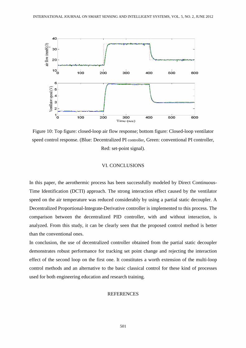
decoupler using IMC tuning rules. It is apparent from these figures that the proposed
decentralized controllers provide a good performance. Their robustness and their effectiveness
are confirmed by the elimination of the interaction effect on the air temperature variable
compared to the controller without decoupler. It is obvious that the proposed controller
affords a good robust performance consistently. We noted that there is no change in the
behavior of the second loop parameters controlled by the PI with and without static decoupler.
This can be justified by the fact that this loop is not infected by the first one represented by
the air temperature and the heater grid. Which confirms quite the interaction test result
obtained in section II.
Figure 10: Top figure: closed-loop air temperature response; bottom figure: Closed-loop
heater grid control response. (Blue: Decentralized PID controller, Green: conventional PID
controller, Red: set-point signal).
INTERNATIONAL JOURNAL ON SMART SENSING AND INTELLIGENT SYSTEMS, VOL. 5, NO. 2, JUNE 2012
501
Figure 10: Top figure: closed-loop air flow response; bottom figure: Closed-loop ventilator
speed control response. (Blue: Decentralized PI controller, Green: conventional PI controller,
Red: set-point signal).
VI. CONCLUSIONS
In this paper, the aerothermic process has been successfully modeled by Direct Continuous-
Time Identification (DCTI) approach. The strong interaction effect caused by the ventilator
speed on the air temperature was reduced considerably by using a partial static decoupler. A
Decentralized Proportional-Integrate-Derivative controller is implemented to this process. The
comparison between the decentralized PID controller, with and without interaction, is
analyzed. From this study, it can be clearly seen that the proposed control method is better
than the conventional ones.
In conclusion, the use of decentralized controller obtained from the partial static decoupler
demonstrates robust performance for tracking set point change and rejecting the interaction
effect of the second loop on the first one. It constitutes a worth extension of the multi-loop
control methods and an alternative to the basic classical control for these kind of processes
used for both engineering education and research training.
REFERENCES

M. Ramzi and H. Youlal, Continuous Time Identification and Decentralized PID Controller of an Aerothermic Process
502
[1] M. Ramzi, H. Youlal and M. Haloua, "State Space Model Predictive Control of an
Aerothermic Process with Actuators Constraints," Intelligent Control and Automation, Vol. 3
No. 1, 2012, pp. 50-58.
[2] N. Bennis, J. Duplaix, G. Enéa, M. Haloua, H. Youlal, “Greenhouse climate modelling
and robust control”, Computers and Electronics in Agriculture, 2008, Vol. 61, pp. 96-107.
[3] M. Nachidi, F. Rodriguez, F. Tadeo, J.L. Guzmanb, “Takagi-Sugeno control of nocturnal
temperature in greenhouses using air heating”, ISA Transactions, 2011, Vol. 50, pp. 315-320.
[4] R.F. Escobar, et al., “Sensor fault detection and isolation via high-gain observers:
Application to a double-pipe heat exchanger”, ISA Transactions, Volume 50, Issue 3, July
2011, pp. 480-486.
[5] M.F. Rahmat , N.A. Mohd Subha, Kashif M.Ishaq and N. Abdul Wahab, “Modeling and
controller design for the VVS-400 pilot scale heating and ventillation system”, International
journal on smart sensing and intelligent systems, December 2009, Vol. 2, No. 4, pp. 579-601.
[6] E. Yesil, M.Guzelkaya, I.Eksin, O. A. Tekin, “Online Tuning of Set-point Regulator with
a Blending Mechanism Using PI Controller”. Turk J Elec Engin, 2008, Vol.16, No. 2, pp.
143-157
[7] T. Kealy, A. O’Dwyer, “Closed Loop Identification of a First Order plus Dead Time
Process Model under PI Control”, Proceedings of the Irish Signals and Systems Conference,
University College, Cork, 2002, pp. 9-14.
[8] R. Mooney and A. O’Dwyer, “A case study in modeling and process control: the control
of a pilot scale heating and ventilation system”, Proceedings of IMC-23; the 23rd
International Manufacturing Conference, University of Ulster, Jordanstown, August, 2006,
pp. 123-130.
[9] H.L. Ho, A.B. Rad, C.C. Chan and Y.K. Wong, “Comparative studies of three adaptive
controllers”, ISA Transactions 38, 1999, pp 43-53.
[10] D.M. de la Pena, D.R. Ramirez, E.F. Camacho, T. Alamo, “Application of an explicit
min-max MPC to a scaled laboratory process”, Control Eng. Practice, Vol. 13, No. 12, 2005,
pp. 1463-1471.
[11] Manual for ERD004000 Flow and Temperature process, 78990 ELANCOURT,
FRANCE, 2008.
[12] H. Garnier, M. Gilson, T. Bastogne, and M. Mensler, “CONTSID toolbox: a software
support for continuous-time data-based modelling. In Identification of continuous time
models from sampled data”, H.Garnier and L. Wang (Eds.), Springer, London, 2008, pp. 249-
290.
INTERNATIONAL JOURNAL ON SMART SENSING AND INTELLIGENT SYSTEMS, VOL. 5, NO. 2, JUNE 2012
503
[13] G. P. Rao and H. Unbehauen, “Identification of continuous time systems” IEE
Proceedings Control Theory and Appl, March 2006, 153 No. 2, pp. 185-220
[14] V. Laurain, M. Gilson, H. Garnier, and P.C. Young. “Refined instrumental variable
methods for identification of Hammerstein continuous-time Box-Jenkins models”, IEEE
Conference on Decision and Control (CDC'2008) , Cancun (Mexico) , December 2008, pp.
1386-1391
[15] Ljung, L. “Initialisation aspects for subspace and output error identification methods”,
European Control Conference (ECC2003), Cambridge (U.K.), December 2003.
[16] H. Garnier, L. Wang, and P.C. Young, “Direct Identification of Continuous-time Models
from Sampled Data: Issues, Basic Solutions and Relevance in Identification of continuous-
time models from sampled data”, Springer, London, 2008, pp. 1-29.
[17] Hugues Garnier, “Data-based continuous-time modelling of dynamic systems”, 4th
International Symposium on Advanced Control of Industrial Processes, Adconip China 2011,
pp. 146-153
[18] V. Laurain, M. Gilson, R. Toth, H. Garnier, “Direct identification of continuous-time
LPV models”, American Control Conference, 2011, pp. 159-164
[19] Young, P.C. “An instrumental variable method for real time identification of a noisy
process”. Automatica, 6, 1970, pp. 271-287.
[20] Young. P.C, “Recursive Estimation and Time-Series Analysis”, Springer-Verlag, Berlin,
1984.
[21] Tham, M.T. (1999). “Multivariable Control: An Introduction to Decoupling Control”.
Department of Chemical and Process Engineering, University of Newcastle upon Tyne.
[22] Dale E. Seborg, Thomas F. Edgard, Duncan A. Mellichamp, “Process dynamics and
control”, Second edition, 2004 John Wiley & sons, pp. 473-502
[23] William Y. Svrcek, Donald P. Mahoney, Brent R. Young, “A Real-Time Approach to
Process Control”, Second Edition, 2006, John Wiley & Sons Ltd, pp. 215-234
[24] Branislav T. Jevtovica, Miroslav R. Matausek, “PID controller design of TITO system
based on ideal decoupler”, Journal of Process Control, 2010, Vol. 20, pp. 869–876
[25] T. Nguyen L. Vu and M. Lee “Independent design of multi-loop PI/PID controllers for
interacting multivariable processes”, Journal of Process Control 20, 2010, pp. 922–933
[26] Guillermo J., Silva Aniruddha Datta and S.R Bhattacharyya, “PID Controllers for Time-
Delay Systems”, 2005 Birkhauser Boston, pp. 1-19
Recommended