1/ 13
A Wiener-Hopf Monte Carlo simulation technique for Lévy processes
A Wiener-Hopf Monte Carlo simulation technique forLévy processes
A. E. Kyprianou, J. C. Pardo and K. van Schaik
Department of Mathematical Sciences, University of Bath

2/ 13
A Wiener-Hopf Monte Carlo simulation technique for Lévy processes
Motivation
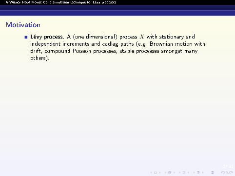
Lévy process. A (one dimensional) process X with stationary andindependent increments and cadlag paths (e.g. Brownian motion withdrift, compound Poisson processes, stable processes amongst manyothers).
Goal of this talk. Present Monte Carlo simulation technique for problemsthat fundamentally depend on the joint distribution
P (Xt ∈ dx, Xt ∈ dy)
where Xt := sups≤tXs.
Example: barrier options in Lévy market. Value of a European up-and-outbarrier option with expiry date T and barrier b is of the form
e−rTEs(f(ST )1{ST≤b})
where S = exp(X), ST = supu≤T Su and f is some nice function.
Other motivations from queuing theory, population models etc.
2/ 13
A Wiener-Hopf Monte Carlo simulation technique for Lévy processes
Motivation
Lévy process. A (one dimensional) process X with stationary andindependent increments and cadlag paths (e.g. Brownian motion withdrift, compound Poisson processes, stable processes amongst manyothers).
Goal of this talk. Present Monte Carlo simulation technique for problemsthat fundamentally depend on the joint distribution
P (Xt ∈ dx, Xt ∈ dy)
where Xt := sups≤tXs.
Example: barrier options in Lévy market. Value of a European up-and-outbarrier option with expiry date T and barrier b is of the form
e−rTEs(f(ST )1{ST≤b})
where S = exp(X), ST = supu≤T Su and f is some nice function.
Other motivations from queuing theory, population models etc.

3/ 13
A Wiener-Hopf Monte Carlo simulation technique for Lévy processes
Facts from Wiener-Hopf theory
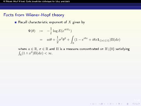
Recall characteristic exponent of X given by
Ψ(θ) := −1
tlogE(eiθXt)
= aiθ +1
2σ2θ2 +
ZR(1− eiθx + iθx1{|x|≤1})Π(dx)
where a ∈ R, σ ∈ R and Π is a measure concentrated on R\{0} satisfyingRR(1 ∧ x2)Π(dx) <∞.
Wiener-Hopf factorisation: one can always decompose
q + Ψ(θ) = κ+(q,−iθ)× κ−(q, iθ)
such that
E(eiθXeq ) =κ+(q, 0)
κ+(q,−iθ) and E(eiθXeq ) =
κ−(q, 0)
κ−(q, iθ)
where eq is an independent and exponentially distributed random variablewith rate q > 0 and Xt := infs≤tXs. (Recall Xt := sups≤tXs.)
3/ 13
A Wiener-Hopf Monte Carlo simulation technique for Lévy processes
Facts from Wiener-Hopf theory
Recall characteristic exponent of X given by
Ψ(θ) := −1
tlogE(eiθXt)
= aiθ +1
2σ2θ2 +
ZR(1− eiθx + iθx1{|x|≤1})Π(dx)
where a ∈ R, σ ∈ R and Π is a measure concentrated on R\{0} satisfyingRR(1 ∧ x2)Π(dx) <∞.
Wiener-Hopf factorisation: one can always decompose
q + Ψ(θ) = κ+(q,−iθ)× κ−(q, iθ)
such that
E(eiθXeq ) =κ+(q, 0)
κ+(q,−iθ) and E(eiθXeq ) =
κ−(q, 0)
κ−(q, iθ)
where eq is an independent and exponentially distributed random variablewith rate q > 0 and Xt := infs≤tXs. (Recall Xt := sups≤tXs.)
4/ 13
A Wiener-Hopf Monte Carlo simulation technique for Lévy processes
Facts from Wiener-Hopf theory
In particular,
Xeqd= Sq + Iq
where Sq is independent of Iq and they are respectively equal indistribution to Xeq and Xeq
.
So:(Xeq , Xeq )
d= (Sq + Iq, Sq).
Q1. For what LP's can we indeed sample from Sq and Iq?
Recent advances: there are many new examples of Lévy processes (withtwo-sided jumps) emerging for which su�cient analytical structure is inplace in order to sample from the two distributions Xeq and Xeq
. (β-Lévy
processes, Lamperti-stable processes, Hypergeometric Lévy processes, · · · ).Q2. How do we get from the random time eq to the �xed time t we areafter?
Put i.i.d. exponentials 'after each other' to construct 'stochastic time grid'and make use of stat. indep. increments of X.
4/ 13
A Wiener-Hopf Monte Carlo simulation technique for Lévy processes
Facts from Wiener-Hopf theory
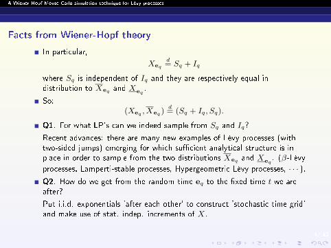
In particular,
Xeqd= Sq + Iq
where Sq is independent of Iq and they are respectively equal indistribution to Xeq and Xeq
.
So:(Xeq , Xeq )
d= (Sq + Iq, Sq).
Q1. For what LP's can we indeed sample from Sq and Iq?
Recent advances: there are many new examples of Lévy processes (withtwo-sided jumps) emerging for which su�cient analytical structure is inplace in order to sample from the two distributions Xeq and Xeq
. (β-Lévy
processes, Lamperti-stable processes, Hypergeometric Lévy processes, · · · ).
Q2. How do we get from the random time eq to the �xed time t we areafter?
Put i.i.d. exponentials 'after each other' to construct 'stochastic time grid'and make use of stat. indep. increments of X.
4/ 13
A Wiener-Hopf Monte Carlo simulation technique for Lévy processes
Facts from Wiener-Hopf theory
In particular,
Xeqd= Sq + Iq
where Sq is independent of Iq and they are respectively equal indistribution to Xeq and Xeq
.
So:(Xeq , Xeq )
d= (Sq + Iq, Sq).
Q1. For what LP's can we indeed sample from Sq and Iq?
Recent advances: there are many new examples of Lévy processes (withtwo-sided jumps) emerging for which su�cient analytical structure is inplace in order to sample from the two distributions Xeq and Xeq
. (β-Lévy
processes, Lamperti-stable processes, Hypergeometric Lévy processes, · · · ).Q2. How do we get from the random time eq to the �xed time t we areafter?
Put i.i.d. exponentials 'after each other' to construct 'stochastic time grid'and make use of stat. indep. increments of X.

5/ 13
A Wiener-Hopf Monte Carlo simulation technique for Lévy processes
'Stochastic time grid'1
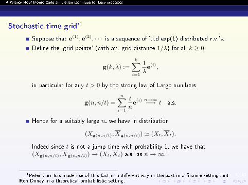
Suppose that e(1), e(2), · · · is a sequence of i.i.d exp(1) distributed r.v.'s.
De�ne the 'grid points' (with av. grid distance 1/λ) for all k ≥ 0:
g(k, λ) :=
kXi=1
1
λe(i),
in particular for any t > 0 by the strong law of Large numbers
g(n, n/t) =
nXi=1
t
ne(i) n→∞−→ t a.s.
Hence for a suitably large n, we have in distribution
(Xg(n,n/t), Xg(n,n/t)) ' (Xt, Xt).
Indeed since t is not a jump time with probability 1, we have that(Xg(n,n/t), Xg(n,n/t))→ (Xt, Xt) a.s. as n→∞.
This + facts from W-H theory from previous slide yields main result:
1Peter Carr has made use of this fact in a di�erent way in the past in a �nance setting andRon Doney in a theoretical probabilistic setting.

5/ 13
A Wiener-Hopf Monte Carlo simulation technique for Lévy processes
'Stochastic time grid'1
Suppose that e(1), e(2), · · · is a sequence of i.i.d exp(1) distributed r.v.'s.
De�ne the 'grid points' (with av. grid distance 1/λ) for all k ≥ 0:
g(k, λ) :=kXi=1
1
λe(i),
in particular for any t > 0 by the strong law of Large numbers
g(n, n/t) =
nXi=1
t
ne(i) n→∞−→ t a.s.
Hence for a suitably large n, we have in distribution
(Xg(n,n/t), Xg(n,n/t)) ' (Xt, Xt).
Indeed since t is not a jump time with probability 1, we have that(Xg(n,n/t), Xg(n,n/t))→ (Xt, Xt) a.s. as n→∞.
This + facts from W-H theory from previous slide yields main result:
1Peter Carr has made use of this fact in a di�erent way in the past in a �nance setting andRon Doney in a theoretical probabilistic setting.

6/ 13
A Wiener-Hopf Monte Carlo simulation technique for Lévy processes
Main result
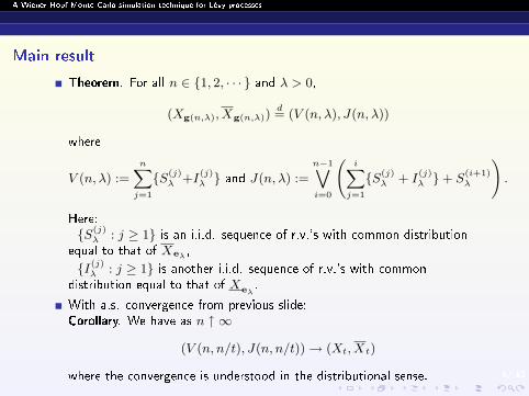
Theorem. For all n ∈ {1, 2, · · · } and λ > 0,
(Xg(n,λ), Xg(n,λ))d= (V (n, λ), J(n, λ))
where
V (n, λ) :=
nXj=1
{S(j)λ +I
(j)λ } and J(n, λ) :=
n−1_i=0
iX
j=1
{S(j)λ + I
(j)λ }+ S
(i+1)λ
!.
Here:- {S(j)
λ : j ≥ 1} is an i.i.d. sequence of r.v.'s with common distributionequal to that of Xeλ ,
- {I(j)λ : j ≥ 1} is another i.i.d. sequence of r.v.'s with common
distribution equal to that of Xeλ.
With a.s. convergence from previous slide:Corollary. We have as n ↑ ∞
(V (n, n/t), J(n, n/t))→ (Xt, Xt)
where the convergence is understood in the distributional sense.
6/ 13
A Wiener-Hopf Monte Carlo simulation technique for Lévy processes
Main result
Theorem. For all n ∈ {1, 2, · · · } and λ > 0,
(Xg(n,λ), Xg(n,λ))d= (V (n, λ), J(n, λ))
where
V (n, λ) :=
nXj=1
{S(j)λ +I
(j)λ } and J(n, λ) :=
n−1_i=0
iX
j=1
{S(j)λ + I
(j)λ }+ S
(i+1)λ
!.
Here:- {S(j)
λ : j ≥ 1} is an i.i.d. sequence of r.v.'s with common distributionequal to that of Xeλ ,
- {I(j)λ : j ≥ 1} is another i.i.d. sequence of r.v.'s with common
distribution equal to that of Xeλ.
With a.s. convergence from previous slide:Corollary. We have as n ↑ ∞
(V (n, n/t), J(n, n/t))→ (Xt, Xt)
where the convergence is understood in the distributional sense.

7/ 13
A Wiener-Hopf Monte Carlo simulation technique for Lévy processes
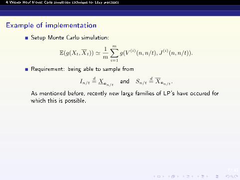
Example of implementation
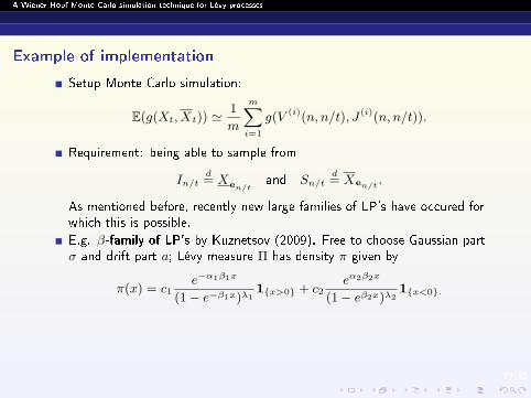
Setup Monte Carlo simulation:
E(g(Xt, Xt)) '1
m
mXi=1
g(V (i)(n, n/t), J(i)(n, n/t)).
Requirement: being able to sample from
In/td= Xen/t
and Sn/td= Xen/t .
As mentioned before, recently new large families of LP's have occured forwhich this is possible.
E.g. β-family of LP's by Kuznetsov (2009). Free to choose Gaussian partσ and drift part a; Lévy measure Π has density π given by
π(x) = c1e−α1β1x
(1− e−β1x)λ11{x>0} + c2
eα2β2x
(1− eβ2x)λ21{x<0}.
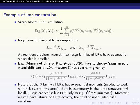
Note that the β-family of LP's has exponential moments (needed to workwith risk neutral measures), there is asymmetry in the jump structure andlocally jumps are stable-like (similarly to e.g. CGMY processes). Moreoverwe can have in�nite or �nite activity, bounded or unbounded pathvariation.
7/ 13
A Wiener-Hopf Monte Carlo simulation technique for Lévy processes
Example of implementation
Setup Monte Carlo simulation:
E(g(Xt, Xt)) '1
m
mXi=1
g(V (i)(n, n/t), J(i)(n, n/t)).
Requirement: being able to sample from
In/td= Xen/t
and Sn/td= Xen/t .
As mentioned before, recently new large families of LP's have occured forwhich this is possible.
E.g. β-family of LP's by Kuznetsov (2009). Free to choose Gaussian partσ and drift part a; Lévy measure Π has density π given by
π(x) = c1e−α1β1x
(1− e−β1x)λ11{x>0} + c2
eα2β2x
(1− eβ2x)λ21{x<0}.
Note that the β-family of LP's has exponential moments (needed to workwith risk neutral measures), there is asymmetry in the jump structure andlocally jumps are stable-like (similarly to e.g. CGMY processes). Moreoverwe can have in�nite or �nite activity, bounded or unbounded pathvariation.

8/ 13
A Wiener-Hopf Monte Carlo simulation technique for Lévy processes
Example of implementation
Kuznetsov uses that the characteristic exponent of X can be extended asa meromorphic function, together with analytical techniques, to identifythe W-H factors and derive e.g.
P (Xeq ∈ dx) =
0@Xn≤0
knζneζnx
1A dx,
where the ζn's are (real) zeros of z 7→ q + Ψ(z) and have to be foundnumerically.
A similar expression for P (Xeq∈ dx)
9/ 13
A Wiener-Hopf Monte Carlo simulation technique for Lévy processes
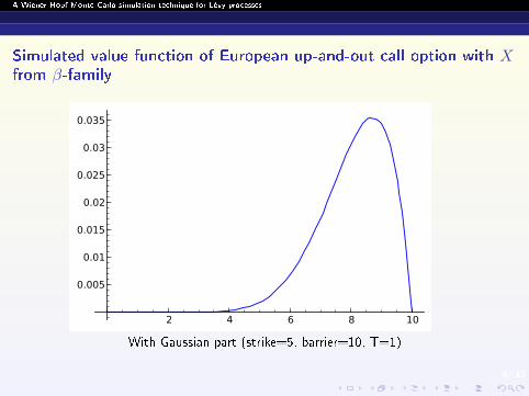
Simulated value function of European up-and-out call option with Xfrom β-family
2 4 6 8 10
0.005
0.01
0.015
0.02
0.025
0.03
0.035
With Gaussian part (strike=5, barrier=10, T=1)

10/ 13
A Wiener-Hopf Monte Carlo simulation technique for Lévy processes
Simulated value function of European up-and-out call option with Xfrom β-family
2 4 6 8 10
0.005
0.01
0.015
0.02
0.025
0.03
0.035
0.04
Irregular upwards (strike=5, barrier=10, T=1)

11/ 13
A Wiener-Hopf Monte Carlo simulation technique for Lévy processes
Advantages over standard random walk approach
Standard random walk:- in general law of Xt not known, needs to be obtained by numericalFourier inversion.- always produces an atom at 0 when simulating Xt (W-H MC methodproduces atom i� it is really present, i.e. i� X is irregular upwards).- well known bad performance when simulating Xt (misses excursionsbetween grid points), W-H MC method performs signi�cantly better inBrownian motion test case

12/ 13
A Wiener-Hopf Monte Carlo simulation technique for Lévy processes
W-H MC method vs. random walk: P (X1 ≤ z) where X is BM; n =number of time steps (for r.w. 2n time steps)

13/ 13
A Wiener-Hopf Monte Carlo simulation technique for Lévy processes
W-H MC method vs. random walk: P (X1 ≤ z1, X1 ≥ z2) where X isBM; 1000 time steps (for r.w. 2000 time steps)
Recommended