A TWO-LEVEL DISCRETIZATION METHOD FOR THE
STREAMFUNCTION FORM OF THE NAVIER-STOKES
EQUATIONS
by
Faisal Abdulkareem Fairag
BS, King Fahd University of Petroulem and Minerals, 1987
MS, King Fahd University of Petroulem and Minerals, 1989
MA, University of Pittsburgh,1994
Submitted to the Graduate Faculty of
Arts and Sciences in partial fulfillment
of the requirements for the degree of
Doctor of Philosophy
University of Pittsburgh
1998
UNIVERSITY OF PITTSBURGH
FACULTY OF ARTS AND SCIENCES
This dissertation was presented
by
Faisal Abdulkareem Fairag
It was defended on
February 5, 1998
and approved by
Charles A. Hall, Ph.D.Professor of Mathematics
D. J. Hebert, Ph.D.Professor of Mathematics
Patrick Smolinski, Ph.D.Professor of Mechanical Engineering
William J. Layton, Ph.D.Professor of MathematicsCommittee chairperson
ii

A TWO-LEVEL DISCRETIZATION METHOD FOR THE
STREAMFUNCTION FORM OF THE NAVIER-STOKES
EQUATIONS
Faisal Abdul-Karim Fairag,PhD
University of Pittsburgh, 1998
ABSTRACT : We analyze a two-level finite element method for the streamfunc-
tion formulation of the Navier-Stokes equations. This report presents the two-level
algorithm and a priori error analysis for the case of conforming elements. The stream-
function formulation in two dimensions has the great advantages that one solves for
only a single scalar variable rather than a coupled system. Further, the incompressible
constraint is automatically satisfied so there are no compatibility conditions between
velocity and pressure spaces. The disadvantage is that the linear system, though
small, arises from a fourth order problem so it can be very ill conditioned. The
nonlinear system is also, at higher Reynolds numbers, very sensitive to small pertur-
bations. The two-level algorithm consists of solving a small nonlinear system on the
coarse mesh, then solving a large linear system on the fine mesh. The basic results
states that the error between the coarse and fine meshes are related superlinearly.
FORTRAN programs for this algorithm and a complete discussion of these pro-
grams are included. These programs are used to solve the Navier-Stokes equations
with a known solution in a rectangular domain for a range of Reynolds numbers to
compare one level vs. two level methods in terms of computer time. Also, we solve
the driven flow in a square cavity. These flows have been widely used as test cases
for validating incompressible fluid dynamics algorithms. Streamfunction contours are
displayed showing the main features of the flow.
iii

A posteriori error estimator for the two-level algorithm is derived which can be
used as an indicator for an assessment of the reliability of the results.
iv

To my parents
v

Acknowledgments
Praise be to Allah, Lord of the worlds, the Almighty, with whose gracious help it
was possible to accomplish this task. I wish to express my sincere appreciation and
deep gratitude to my dissertation advisor, Professor William Layton for his generous
support, encouragement and suggesting the topic of this dissertation. I thank him
for many stimulating discussions and introducing me to a field where he has made so
many significant contributions. I am thankful to my committee members, to Professor
D. J. Hebert for reading the manuscript in draft form and pointing out to me various
misprints and suggestions. I thank Professor C. Hall and P. Smolinski for suggesting
to add a remark in Section(5.4) and a paragraph about the reduced basis method in
the introduction. This work was supported by King Fahd University of Petroleum
and Minerals under sponsorship 152-SD.
I am thankful to Professor L. Tobiska for reading and commenting on chapter
2. I thank Professor J. E. Akin, Rice University, Houston, Texas for permission
to reproduce Figure(5 .9) taken from [2] and to Professor U. Ghia for permission to
reproduce Figure(5 .8) taken from [31]. I am truly thankful to Professor F. Schieweck,
for generously providing the postscript file of Figure(5 .4) taken from [63]. I thank
Professor J. Xu for referring me to many references related to Chapter 2. I wish to
acknowledge the fruitful discussions by Professor J. Maubach and V. Ervin on some
computational aspects of this dissertation. I thank Professor V. John for providing
me some references related to chapter 3.
It is my great pleasure to thank my wife, Wejdan Iskander, for spending endless
days and nights typesetting the dissertation and for long-suffering, patience and un-
derstanding which made it possible. It is a great privilege and pleasure to thank my
vi

parents, Fatemah Fairag and Abdul-karim Fairag, to whom this work is dedicated.
From childhood and on, I have received their blessings, long-support and encourage-
ments to continue my education.
vii

Contents
1 Introduction 1
1.1 Motivations . . . . . . . . . . . . . . . . . . . . . . . . . . . . . . . . 2
1.2 Navier-Stokes Equations . . . . . . . . . . . . . . . . . . . . . . . . . 4
1.3 Streamfunction Equation . . . . . . . . . . . . . . . . . . . . . . . . . 6
1.4 Two-Level Idea . . . . . . . . . . . . . . . . . . . . . . . . . . . . . . 8
1.5 A Model Problem and Chapters Description . . . . . . . . . . . . . . 10
2 A’ Priori Error Analysis 14
2.1 Introduction . . . . . . . . . . . . . . . . . . . . . . . . . . . . . . . . 15
2.2 Notations and Preliminaries . . . . . . . . . . . . . . . . . . . . . . . 16
2.3 Two Weak Formulations . . . . . . . . . . . . . . . . . . . . . . . . . 18
2.4 Two Level Method . . . . . . . . . . . . . . . . . . . . . . . . . . . . 22
2.5 The Error Bound . . . . . . . . . . . . . . . . . . . . . . . . . . . . . 27
2.6 Summary . . . . . . . . . . . . . . . . . . . . . . . . . . . . . . . . . 36
3 A Posteriori Error Estimator 37
3.1 Introduction . . . . . . . . . . . . . . . . . . . . . . . . . . . . . . . . 38
3.2 Notations and Preliminaries . . . . . . . . . . . . . . . . . . . . . . . 39
3.3 Error Analysis . . . . . . . . . . . . . . . . . . . . . . . . . . . . . . . 44
viii
4 Implementation of the Two-Level FEM 55
4.1 Introduction . . . . . . . . . . . . . . . . . . . . . . . . . . . . . . . . 56
4.2 Notations and Arrays . . . . . . . . . . . . . . . . . . . . . . . . . . . 57
4.3 Mesh Generation . . . . . . . . . . . . . . . . . . . . . . . . . . . . . 60
4.4 Affine Mapping . . . . . . . . . . . . . . . . . . . . . . . . . . . . . . 67
4.5 Basis Functions for Morley Element . . . . . . . . . . . . . . . . . . . 71
4.6 Basis Function for Bogner-Fox-Schmit Element . . . . . . . . . . . . . 76
4.7 Discretizing the Continuous Problem . . . . . . . . . . . . . . . . . . 89
4.8 The Solution of F (C) = 0 . . . . . . . . . . . . . . . . . . . . . . . . 90
4.9 Computation of the Jacobian . . . . . . . . . . . . . . . . . . . . . . 92
4.10 Calculation of the Load Vector . . . . . . . . . . . . . . . . . . . . . . 109
4.11 Storage of the Jacobian . . . . . . . . . . . . . . . . . . . . . . . . . 111
4.12 Boundary Conditions Contribution . . . . . . . . . . . . . . . . . . . 114
4.13 Solving the Linear System . . . . . . . . . . . . . . . . . . . . . . . . 115
4.14 COARSE-LEVEL-SOLVE Subroutine . . . . . . . . . . . . . . . . . . 119
4.15 FINE-LEVEL-SOLVE Subroutine . . . . . . . . . . . . . . . . . . . . 119
5 Numerical Tests 126
5.1 Introduction . . . . . . . . . . . . . . . . . . . . . . . . . . . . . . . . 127
5.2 Accuracy Two Level Method vs. One Level Method . . . . . . . . . . 127
5.3 Robustness: Test Problem for Different Reynolds Numbers . . . . . . 133
5.4 Meshes Scaling Test . . . . . . . . . . . . . . . . . . . . . . . . . . . . 139
5.5 The Driven Cavity Problem . . . . . . . . . . . . . . . . . . . . . . . 143
A FORTRAN 90 Program Using Morley Element 151
B FORTRAN 77 Program Using Bogner-Fox-Schmit Element 182
ix
C MATLAB and M-files 219
D Data Files 238
6 Bibliography 262
x

List of Tables
2 .1 Scaling of two level finite elements . . . . . . . . . . . . . . . . . . . . 26
5 .1 One level method. . . . . . . . . . . . . . . . . . . . . . . . . . . . . . 130
5 .2 Two level method. . . . . . . . . . . . . . . . . . . . . . . . . . . . . 130
5 .4 Values for streamline contours in Figure ( 5 .3). . . . . . . . . . . . . 134
5 .3 Two level for test problem. . . . . . . . . . . . . . . . . . . . . . . . . 135
5 .5 L2-error, H1-error and H2-error of ψ for different pairs (H, h). . . . . 141
5 .6 Results for u-velocity along the vertical line x = 0.5 . . . . . . . . . . 145
5 .7 Results for v-velocity along the horizontal line y = 0.5 . . . . . . . . . 145
5 .8 Two level for cavity flow . . . . . . . . . . . . . . . . . . . . . . . . . 146
xi

List of Figures
2 .1 The Argyris triangular element . . . . . . . . . . . . . . . . . . . . . 24
2 .2 The Clough-Tocher triangular element . . . . . . . . . . . . . . . . . 25
2 .3 The Bogner-Fox-Schmit rectangular element . . . . . . . . . . . . . . 25
3 .1 The Clough-Tocher triangle element . . . . . . . . . . . . . . . . . . . 44
3 .2 Bogner-Fox-Schmit rectangular element . . . . . . . . . . . . . . . . . 46
4 .1 Triangles labeling . . . . . . . . . . . . . . . . . . . . . . . . . . . . . 61
4 .2 Global node labeling . . . . . . . . . . . . . . . . . . . . . . . . . . . 62
4 .3 Local node ordering . . . . . . . . . . . . . . . . . . . . . . . . . . . . 62
4 .4 Rectangles labeling . . . . . . . . . . . . . . . . . . . . . . . . . . . . 66
4 .5 Global node ordering . . . . . . . . . . . . . . . . . . . . . . . . . . . 67
4 .6 Local node ordering . . . . . . . . . . . . . . . . . . . . . . . . . . . . 68
4 .7 The reference Triangle . . . . . . . . . . . . . . . . . . . . . . . . . . 68
4 .8 The reference rectangle . . . . . . . . . . . . . . . . . . . . . . . . . . 70
4 .9 Local basis functions for Morley element . . . . . . . . . . . . . . . . 75
4 .10 Local basis functions for Bogner-Fox-Schmit elements (φ1 · · · φ6 ) . . . 86
4 .11 Local basis functions for Bogner-Fox-Schmit elements (φ7 · · · φ12) . . . 87
4 .12 Local basis functions for Bogner-Fox-Schmit elements (φ13 · · · φ16) . . 88
4 .13 el Triangle . . . . . . . . . . . . . . . . . . . . . . . . . . . . . . . . . 93
xii
4 .14 Nonzero element location for lx=2,3,4,5 . . . . . . . . . . . . . . . . . 113
4 .15 Bandwidth of the Jacobian matrix . . . . . . . . . . . . . . . . . . . . 116
4 .16 Triangle g . . . . . . . . . . . . . . . . . . . . . . . . . . . . . . . . . 122
4 .17 Nonzero entries for (H, h) = (12, 1
4), (1
3, 1
6) . . . . . . . . . . . . . . . . 125
5 .1 Streamlines for h = 18, 1
14, 1
16with Re=10 and the corresponding 3-D
graphs using one level method . . . . . . . . . . . . . . . . . . . . . . 131
5 .2 Streamlines for (H, h) = (14, 1
8), (1
7, 1
14), (1
8, 1
16) with Re=10 and the cor-
responding 3-D graphs using two level method . . . . . . . . . . . . . 132
5 .3 Streamlines for H = 116
, h = 132
using Bogner-Fox-Schmit element. . . 136
5 .4 Streamlines for h = 164
(courtesy F. Schieweck [63]). . . . . . . . . . . 137
5 .5 Streamlines for H = 116
, h = 132
using Morley element. . . . . . . . . . 138
5 .6 Streamlines for (H, h) = (14, 1
8), (1
4, 1
8), (1
4, 1
16) and (1
4, 1
20). . . . . . . . . 142
5 .7 Streamlines for H = 116
, h = 132
with different values of Re numbers
using two level method . . . . . . . . . . . . . . . . . . . . . . . . . . 147
5 .8 Ghia-Ghia-Shin’s streamlines, 129× 129, (courtesy U. Ghia [31]). . . 148
5 .9 (a),(c) Streamlines for cavity flow using two level method, (b),(d)
Akin’s streamlines, a mesh of 40× 40 elements, (courtesy J. Akin [2]). 149
5 .10 (above)u-velocity lines through the vertical line x = 0.5, (below) v-
velocity lines through the horizontal line y = 0.5. . . . . . . . . . . . 150
xiii

Chapter 1
Introduction
1
2
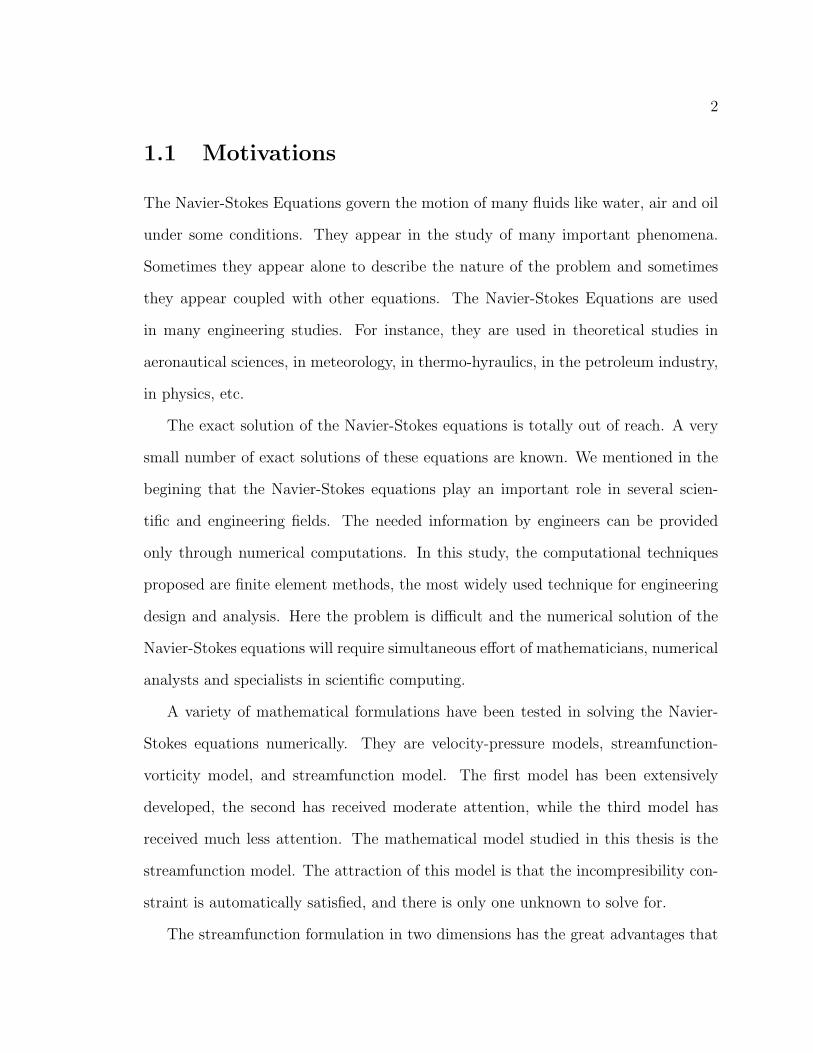
1.1 Motivations
The Navier-Stokes Equations govern the motion of many fluids like water, air and oil
under some conditions. They appear in the study of many important phenomena.
Sometimes they appear alone to describe the nature of the problem and sometimes
they appear coupled with other equations. The Navier-Stokes Equations are used
in many engineering studies. For instance, they are used in theoretical studies in
aeronautical sciences, in meteorology, in thermo-hyraulics, in the petroleum industry,
in physics, etc.
The exact solution of the Navier-Stokes equations is totally out of reach. A very
small number of exact solutions of these equations are known. We mentioned in the
begining that the Navier-Stokes equations play an important role in several scien-
tific and engineering fields. The needed information by engineers can be provided
only through numerical computations. In this study, the computational techniques
proposed are finite element methods, the most widely used technique for engineering
design and analysis. Here the problem is difficult and the numerical solution of the
Navier-Stokes equations will require simultaneous effort of mathematicians, numerical
analysts and specialists in scientific computing.
A variety of mathematical formulations have been tested in solving the Navier-
Stokes equations numerically. They are velocity-pressure models, streamfunction-
vorticity model, and streamfunction model. The first model has been extensively
developed, the second has received moderate attention, while the third model has
received much less attention. The mathematical model studied in this thesis is the
streamfunction model. The attraction of this model is that the incompresibility con-
straint is automatically satisfied, and there is only one unknown to solve for.
The streamfunction formulation in two dimensions has the great advantages that

3
one solves for only a single scalar variable rather than a coupled system. Further,
the incompressible constraint is automatically satisfied so there are no compatibility
conditions between velocity and pressure spaces. The disadvantage is that the linear
system, though small, arises from a fourth order problem so it can be very ill posed.
The nonlinear system is also, at higher Reynolds numbers, very sensitive to small
perturbations. Thus global convergence of Newton’s method does not hold. In fact,
in our tests we found that normal Newton iterations did not converge to the solution
of the nonlinear algebraic system for even moderate Reynolds numbers. Further, at
moderate to high Reynolds numbers the linearized system arising from the full New-
ton step is both nonsymmetric and indefinite. We experienced severe difficulties, as
well, in the convergence of generalized conjugate gradient iterations approximating
the solution of the linear problems. These difficulties arose principally when we were
solving the system arising from the usual finite element method to compare it to
the solution of the two level discretization method. In fact, none of the difficulties
mentioned above occur when the two level that we propose and study is used to dis-
cretize the streamfunction formulation of the Navier-Stokes equations: the particular
update is designed specifically to circumvent these difficulties associated with higher
Reynolds numbers. The method begins by calculating a coarse mesh approximate
solution which is interpolated to a fine mesh. Taking a partial linearization about
this coarse mesh approximate solution, and beginning with it as an initial guess, an
update is calculated on the fine mesh by using a partial linearization of the nonlinear
system. The simplest partial linearization is to delete all the nonlinear terms. This
Stokes approximation is clearly hopeless at moderate to high Reynolds numbers. We
selected a partial linearization based upon the associated Oseen problem. The linear
system arising from this problem on the fine mesh, while not symmetric, does have
positive definite symmetric part. It is therefore not surprising that we experienced no

4
difficulty whatsoever in solving the associated linear system by generalized constant
gradient methods. The main thrust of this thesis is to analyze this procedure: What
relationships between the coarse and the fine mesh ensure that the accuracy will be
the same as if the full fine-mesh non linear system were solved to truncation error?
How does one estimate the computational error in this procedure and designed adap-
tive meshes associated with it? Is the solution quality comparable to that obtained
by solving the full nonlinear system? In practical tests what efficiency advantages are
obtained with the new method?
In summary, the purpose of this thesis is to present and study the a priori and a
posteriori error analysis of a new two level finite element method for discretizing the
streamfunction formulation of the Navier-Stokes equations. Moreover, the resulting
methods will be tested on some practical problems.
1.2 Navier-Stokes Equations
Galdi [29, 30] said: ”The Navier-Stokes Equations have been written more than one
hundred seventy years ago. In fact, they were proposed in 1822 by the French engineer
C.M.L.H. Navier upon the basis of a suitable molecular model. It is interesting to
observe. However, the law of interaction between the molecules postulated by Navier
were shortly recognized to be totally inconsistent from the physical point of view for
several materials and, in particular, for liquids. It was only more than twenty years
later that the same equations were rederived by G.H. Stokes (1845) in a quite general
way by means of the theory of continua.”
While the physical model leading to the Navier-Stokes equations is simple, the
situation is different from the mathematical point of view. Actually, the exact solution
of the Navier-Stokes equations is totally out of reach. A very small number of exact
5
solutions of these equations are known. The Navier-Stokes equations can be written
as follows
− 1
Re4 u + u · 5u +5p = f in Ω,
div u = 0 in Ω,
u = 0 on ∂Ω,
where u = u(x, y) is the velocity field evaluated at point x ∈ Ω, Re is the Reynolds
number, p is the pressure field, and Ω is a bounded simply connected domain in R2.
Many researchers believe that the difficulties in getting the exact solution is because
of the nonlinear term u ·5u. Galdi [29, 30] presented an explanation of the difficulties
of the analytical solution of the Navier-Stokes equations. The following paragraph
summarizes his explanation.
First, the Navier-Stokes equations do not satisfy a specific property. He calls this
property a symmetry in u and p. Because of the lack of symmetry in u and p, the
Navier-Stokes equations do not fall in any of the classical categories of equations.
The reason that the Navier-Stokes equations are so difficult is the coupled effect of
the absence of symmetry and of the presence of the nonlinear term. Three types of
problems appear in the mathematical and analytical treatments of these equations.
These problems are existence, uniqueness, and regularity.
Many mathematicians attack the equations to study these problems and present
them in papers and textbooks. One of the most accessible is An Introduction to the
Navier-Stokes Initial Boundary Value Problem by Giovanni P. Galdi [28]. A valuable
source of a systematic and up-to-date investigation of the fundamental properties
of the Navier-Stokes equations is this series of Galdi [28] which is divided into four
volumes.

6
1.3 Streamfunction Equation
We mentioned earlier that the Navier-Stokes equations play an important role in
several scientific and engineering fields. The information needed by engineers can be
provided only through numerical computations.
The mathematical model studied in this thesis is the streamfunction model. For
2D domains, the streamfunction equation can be written as follows
Re−1 42 ψ − ψy 4 ψx + ψx 4 ψy = curl f in Ω,
ψ =∂ψ
∂n= 0 on ∂Ω,
where ψ denotes the streamfunction, f is the given body force, Re is the given
Reynolds number and n represents the outward unit normal to Ω.
It is well known that for the velocity-pressure formulation of the Navier-Stokes
problem the velocity and pressure approximation spaces need to be compatible to
avoid instability. This condition, the Ladyzhenskaya-Babuska-Brezzi condition, arises
from the study of stability and convergence properties of the velocity-pressure formu-
lation of the Navier-Stokes problem. To satisfy this condition we can not pick any
two arbitrary discrete spaces for the velocity and pressure. For example, one idea
of Arnold-Brezzi-Fortin [5] was to increase the number of degrees of freedom of the
velocity element by adding bubble functions. This was done to reduce the space of
pressure or to enrich the space of velocity elements.
Another still unexplored possibility is to explicitly weaken the condition div u = 0
by changing it to
div u = g, (e.g., g = h2 4 p),
when g is a (well-chosen) small function. The first step in this direction has been

7
done in the work of Brezzi-Pitkranta [14]. One use of the streamfunction formulation
avoids completely compatability condition because the pressure is eliminated from
momentum equation to yield a single nonlinear fourth order equation.
This idea of eliminating the pressure and the satisfaction of the continuity equation
are also present in the Divergence Free Finite Element Method (DFFEM) (discussed,
studied and analyzed in [38, 39]). The DFFEM treats the continuity equation as a
constraint, thus the velocity is approximated not from the standard finite element
vector space but from a discretely divergence free element subspace. In DFFEM
approach, the pressures are eliminated from the calculations and the dimension of the
system to be solved is reduced. For this technique to work, however, the underlying
velocity-pressure approximation must still be stable.
A variety of numerical methods are used to solve the Navier-Stokes equations nu-
merically using the streamfunction formulation. Finite difference approach for the
streamfunction formulation was discussed in Goodrich-Gustafson-Halasi [34]. Cayco
and Nicolaides [17, 16] gave a convergence analysis for small data (the case of global
uniqueness) for this formulation of the Navier-Stokes equations. Some numerical ex-
ample using the streamfunction formulation can be found in Betts-Haroutunian [12].
For a nonconforming finite element method, Baker and Jureidini [8] investigated the
use of elements which are required only to be continuos, not continuously differen-
tiable and not to satisfy the boundary conditions with a streamfunction formulation.
Cayco and Nicolaides [16] presented and discussed a new weak form, which is suitable
for analysis of nonconforming finite element approximations. Phillips and Malek [51]
studied the Multidomain Collocation method for the streamfunction formulation of
the Navier-Stokes equation.
The streamfunction formulation is a nonlinear forth order partial differential equa-
tion. The first example of a fourth order partial differential equation is the biharmonic

8
equation, namely,
42ψ = f in Ω,
ψ =∂ψ
∂n= 0 on ∂Ω.
The biharmonic equation models a plate bending problem. The finite element method
for the linear biharmonic equation was discussed and analyzed extensively in [18, 19].
The difficulty that fourth order problems pose from an algorithmic point of view is
that conforming finite element methods require the use of continuously differentiable
finite element functions. There are many elements which satisfy this requirement.
For details concerning these elements and their approximation properties, one may
consult Ciarlet [18, 19].
1.4 Two-Level Idea
The conforming finite element method of the streamfunction formulation requires the
use of finite element functions that are continuously differentiable over Ω; this is a
difficult constraint to satisfy in practice. Furthermore, the use of continuously differ-
entiable finite elements leads to solving a large nonlinear system of equations. The
study of nonconforming methods has received great attention from the desire to avoid
the construction of finite element spaces and their bases that satisfy the C1 continu-
ity requirement. Many nonconforming elements which are applicable for biharmonic
equation is described in [18, 19]. In fact, in our tests we found that nonconforming
elements are much more sensitive for even moderate Reynolds numbers.
Another idea of avoiding the solution of a large nonlinear system of equations
is a two level finite element method. The two level algorithm consists of solving a
9
small nonlinear system on the coarse mesh, then solving a linear system on the fine
mesh. The computed solution from this procedure has the same quality if we solve a
nonlinear system of equations in the fine mesh. The computational attraction of the
methods is that they require the solution of a small system of nonlinear equations
and one large linear system of equations. These types of methods were pioneered by
Xu in [69, 70] for semilinear elliptic problems. The two level discretization methods
have been analyzed for the Navier-Stokes equations by Layton in [41, 44, 42, 40].
Another idea of avoiding the solution of a large nonlinear system of equations is
reduction method that reduces the degree of freedom. The reduced basis method is a
reduction-type method that uses approximating functions that are closely related to
the solution of the differential equation, see, e.g., [3, 54, 55, 4, 56, 27, 60, 58, 59, 50].
For example, two choices of reduced spaces are the Lagrange space and the Taylor
space. In Navier-Stokes equations, the Lagrange space consists of solutions to the
Navier-Stokes equations for different values of the Reynolds number. Hence, all basis
vectors are generated by solving a large nonlinear system. The Taylor space consists
of solution to the Navier-Stokes equations at a given Reynolds number, Re0. The
remaining vectors are obtained by solving the equations that result by differentiating
the Navier-Stokes equations with respect to the Reynolds number and evaluating at
Re0. The computation of the first vector requires the solution of a large nonlinear
system. For the other vectors, a large linear system is to be solved for each vector.
Now, the reduced basis solution is a linear combination of three vectors. This result in
a dense system of equations. This is due to the fact that the reduced basis vectors are
global as opposed to the local basis vectors used in standard finite elements. Hence,
the reduced basis method is feasible only if a very small number of basis vectors are
needed. In the numerical solution of the Navier-Stokes equation, engineers need to
know how globally close the computed solution is to the exact solution. This point

10
shows the need for an error estimator, which must be a posteriori computed from the
computed numerical solution and the given data of the problem. This estimator will
give us an upper bound to the accuracy of the numerical approximation.
1.5 A Model Problem and Chapters Description
We first need to define some function spaces and associated norms. More details
concerning these spaces can be found in [1]. Let Ω be a bounded simply connected
polygonal domain in R2. L2(Ω) is the Hilbert space of Lebesque square integrable
functions with norm ‖ · ‖ and L20(Ω) is the subspaces of L2(Ω) consisting of functions
with zero mean. Let Hm(Ω) be usual Sobolev space consisting of functions which
together with their distributional derivatives up through order m are in L2(Ω). Denote
the norm on Hm(Ω) by ‖ · ‖m. Let Hm0 (Ω) be the completion of C∞
0 (Ω) under
the ‖ · ‖−m norm. We equip Hm0 (Ω) with the seminorm | · |m, which is a norm
equivalent to ‖ · ‖m. Also, the dual of space Hm0 (Ω) is denoted by H−m(Ω), with
norm ‖ · ‖−m. Let [Hm(Ω)]2 be the space Hm(Ω) × Hm(Ω) and [Hm0 (Ω)]2 be the
space Hm0 (Ω)×Hm
0 (Ω) equipped with the following norm.
‖ u ‖m = (‖ u1 ‖2m + ‖ u2 ‖2
m)1/2 and
| u |m = (| u1 |2m + | u2 |2m)1/2
where
u =
u1
u2
.
11
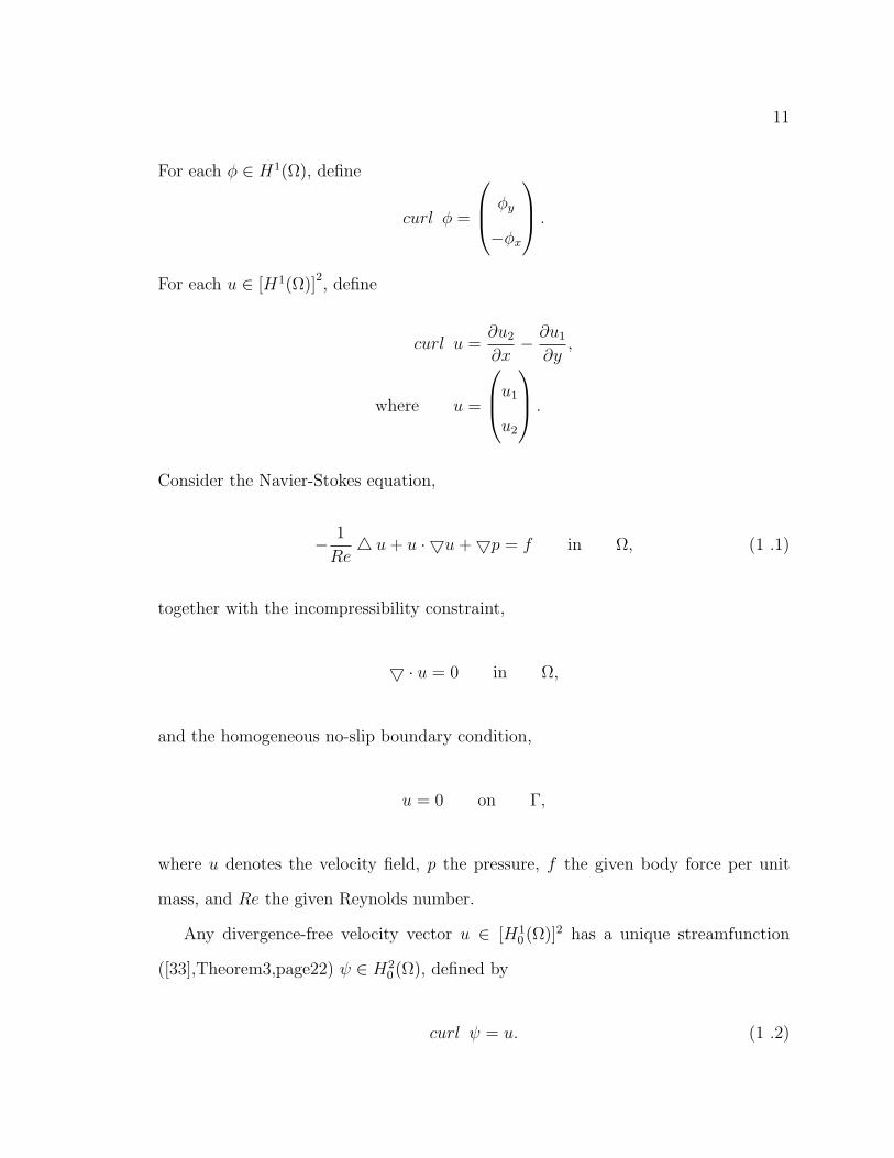
For each φ ∈ H1(Ω), define
curl φ =
φy
−φx
.
For each u ∈ [H1(Ω)]2, define
curl u =∂u2
∂x− ∂u1
∂y,
where u =
u1
u2
.
Consider the Navier-Stokes equation,
− 1
Re4 u + u · 5u +5p = f in Ω, (1 .1)
together with the incompressibility constraint,
5 · u = 0 in Ω,
and the homogeneous no-slip boundary condition,
u = 0 on Γ,
where u denotes the velocity field, p the pressure, f the given body force per unit
mass, and Re the given Reynolds number.
Any divergence-free velocity vector u ∈ [H10 (Ω)]2 has a unique streamfunction
([33],Theorem3,page22) ψ ∈ H20 (Ω), defined by
curl ψ = u. (1 .2)
12
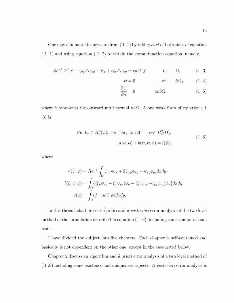
One may eliminate the pressure from ( 1 .1) by taking curl of both sides of equation
( 1 .1) and using equation ( 1 .2) to obtain the streamfunction equation, namely,
Re−1 42 ψ − ψy 4 ψx + ψx + ψx 4 ψy = curl f in Ω, (1 .3)
ψ = 0 on ∂Ω1, (1 .4)
∂ψ
∂n= 0 on∂Ω, (1 .5)
where n represents the outward until normal to Ω. A one weak form of equation ( 1
.3) is
Findψ ∈ H20 (Ω)such that, for all φ ∈ H2
0 (Ω),
a(ψ, φ) + b(ψ, ψ, φ) = l(φ),
(1 .6)
where
a(ψ, φ) = Re−1
∫
Ω
ψxxφxx + 2ψxyφxy + ψyyφyydxdy,
b(ξ, ψ, φ) =
∫
Ω
(ξyψxy − ξxψyy)φy − (ξxψxy − ξyψxx)φxdxdy,
l(φ) =
∫
Ω
(f · curl φ)dxdy.
In this thesis I shall present a priori and a posteriori error analysis of the two level
method of the formulation described in equation ( 1 .6), including some computational
tests.
I have divided the subject into five chapters. Each chapter is self-contained and
basically is not dependent on the other one, except in the case noted below.
Chapter 2 discuss an algorithm and a priori error analysis of a two level method of
( 1 .6) including some existence and uniqueness aspects. A posteriori error analysis is

13
presented in chapter 3. Chapter 4 focuses on the implementation of the finite element
method for the algorithm which was described in chapter 2. In chapter 5 we test the
code described in chapter 4 for a test problem with a known solution and a driven
cavity problem.

Chapter 2
A’ Priori Error Analysis
14

15
2.1 Introduction
Convergence analysis for finite element approximation of the primitive variable for-
mulation of the Navier-Stokes equations has been extensively developed in the last 20
years, see for example [36, 33, 32, 62]. The analogous theory for the streamfunction
formulation for the Navier-Stokes equations has received much less attention. The at-
tractions of the streamfunction formulation are that the incompressibility constraint
is automatically satisfied , the pressure is not present in the weak form and there is
only one scalar unknown to solve for. The standard weak formulation of the stream-
function version first appeared in 1979 in [33]. In this direction, Cayco and Nicolaides
[17, 16] studied a general analysis of convergence for this standard weak formulation
of the Navier-Stokes equations. The standard weak form is unsuitable for derivation
or analysis of nonconforming finite element approximations. For a nonconforming
finite element method, Baker and Jureidini [8] investigated the use of elements which
are required only to be continuous and not to satisfy the boundary conditions with a
nonstandard weak formulation. Their weak formulation extends the standard one by
including appropriate integrals on inter-element boundaries and on the boundary of
the problem domain. Cayco and Nicolaides [16] presented and discussed a new weak
form, which is suitable for analysis of nonconforming finite element approximations.
They discussed this weak form and applied it to three specific nonconforming finite
element schemes.
The discretization of the streamfunction formulation still leads to a problem of
solving a large and ill-conditioned nonlinear systems of algebraic equations. two level
finite element discretization are presently a very promising approach for approxi-
mating the Navier-Stokes equations, see [41]. The computational attraction of the
methods are that they require the solution of only a small system of nonlinear equa-
16
tions on coarse mesh and one linear system of equations on fine mesh. These types
of methods were pioneered by Xu in [69, 70] for semilinear elliptic problems. The
two level discretization methods have been recently analyzed for the Navier-Stokes
equations in [41, 43, 44] and for the streamfunction formulation of the Navier-Stokes
equations in [72]. The methods studied in [72] involve solving a full linearization of
the streamfunction equation on the fine mesh. The purpose of this thesis is to present
and analyze a two level conforming finite element method for discretizing the stream-
function formulation of the Navier-Stokes equations, which requires the solution of a
partial linearization of the streamfunction equation on the fine mesh.
2.2 Notations and Preliminaries
We first need to define some function spaces and associated norms. More detailed
concerning these spaces can be found in [1]. Let Ω be a bounded simply connected
polygonal domain in R2. L2(Ω) is the Hilbert space of Lebesgue square integrable
functions with norm ‖ · ‖0 and L20(Ω) is the subspace of L2(Ω) consisting of functions
with zero mean. Let Hm(Ω) be the usual Sobolev space consisting of functions which
together with their distributional derivatives up through order m are in L2(Ω). Denote
the norm on Hm(Ω) by ‖ · ‖m. Let Hm0 (Ω) be the completion of C∞
0 (Ω) under the
‖ · ‖m norm. We equip Hm0 (Ω) with the seminorm | · |m, which is a norm equivalent to
‖ · ‖m. Also, the dual of space Hm0 (Ω) is denoted by H−m(Ω), with norm ‖ · ‖−m. Let
[Hm(Ω)]2 be the space Hm(Ω)×Hm(Ω) and [Hm0 (Ω)]2 be the space Hm
0 (Ω)×Hm0 (Ω)

17
equipped with the following norm
‖ u ‖m = (‖ u1 ‖2m + ‖ u2 ‖2
m)1/2 and
| u |m = (| u1 |2m + | u2 |2m)1/2 where u =
u1
u2
.
For each φ ∈ H1(Ω), define
curl φ =
φy
−φx
.
For each u ∈ [H1(Ω)]2, define
curl u =∂u2
∂x− ∂u1
∂y, where u =
u1
u2
.
Consider the Navier-Stokes equations describing the flow of an incompressible
fluid:
−Re−1 4 u + (u · 5)u +5p = f, in Ω,
5 · u = 0, in Ω,
u = 0, on ∂Ω,∫
Ω
p dΩ = 0.
(2 .1)
Later, we will state conditions on f and Re−1 guaranteeing the solution to ( 2 .1).
Any divergence-free velocity vector u ∈ [H10 (Ω)]2 has a unique stream function [33,
Theorem3.1,page 22] ψ ∈ H20 (Ω), defined by
curlψ = u.
18
Moreover, the streamfunction ψ satisfies
Re−1 42 ψ − ψy 4 ψx + ψx 4 ψy = curl f, in Ω,
ψ = 0, on ∂Ω,
∂ψ
∂n= 0, on ∂Ω,
(2 .3)
where n represents the outward unit normal to Ω.
2.3 Two Weak Formulations
The standard weak form of equation ( 2 .1) is
Find u ∈ [H10 ]2, p ∈ L2
0(Ω), such that ∀w ∈ [H10 (Ω)]2, q ∈ L2
0(Ω),
Re−1a(u,w) + b(u; u,w) + c(w, p) =< f, w >,
c(u, q) = 0,
(2 .4)
where
a(u,w) =
∫
Ω
5u : 5w,
b(u; v, w) =
∫
Ω
((u · 5)v) · w,
c(w, q) =
∫
Ω
q div w,
(2 .5)
and < ·, · > denotes the duality pairing in L2(Ω). The standard weak form of equation
( 2 .3) is:
Find ψ ∈ H20 (Ω) such that, for all φ ∈ H2
0 (Ω),
a(ψ, φ) + b(ψ; ψ, φ) = l(φ),
(2 .6)

19
where
a(ψ, φ) = Re−1
∫
Ω
4ψ · 4φ,
b(ξ; ψ, φ) =
∫
Ω
4ξ(ψyφx − ψxφy),
l(φ) = (f, curl φ) =
∫
Ω
f · curl φ.
(2 .7)
Another equivalent formulation of equation ( 2 .3), introduced by Cayco and Nico-
laides [16], is:
Find ψ ∈ H20 (Ω) such that, for all φ ∈ H2
0 (Ω),
a0(ψ, φ) + b0(ψ; ψ, φ) = l(φ),
(2 .8)
where
a0(ψ, φ) = Re−1
∫
Ω
ψxxφxx + 2ψxyφxy + ψyyφyy,
b0(ξ; ψ, φ) =
∫
Ω
(ξyψxy − ξxψyy)φy − (ξxψxy − ξyψxx)φx,
l(φ) = (f, curl φ) =
∫
Ω
f · curl φ.
(2 .9)
Conforming element can be used with either ( 2 .6) or ( 2 .8), in this case the
two weak formulations produce identical results because a(ψ, φ) = a0(ψ, φ) and
b(ξ; ψ, φ) = b0(ξ; ψ, φ) for all ψ, φ, ξ ∈ H20 (Ω). However, when using nonconforming
approximation subspaces, ( 2 .8) and ( 2 .6) generate different finite element methods.
Nonconforming elements should be used only with ( 2 .8). To illustrate the reason,
suppose we solve the Stokes problem with the nonconforming Morley triangle, i.e.
the quadratic element whose degrees of freedom are function values at the vertices
and normal derivatives at the midsides. Boundary conditions are imposed by setting
20
all the degrees of freedom at the boundary to be zero. Observe that a necessary and
sufficient condition for the existence of a unique solution to the discrete biharmonic
equation is that the bilinear induces a norm on the trial space. This is not the case
for the Morley space [17]. The following theorem states that the forms ( 2 .4) and
( 2 .6) are equivalent in the sense of having identical solutions. The reason for this is
that the space of curls of H20 (Ω) functions coincides with the space of divergence-free
functions in [H10 (Ω)]2.
The following theorem states that the problems ( 2 .1) and ( 2 .3) are equivalent in
the sense of having identical solutions.
Theorem 2.3.1 ([33]Theorem 2.6,page 120)
Problems ( 2 .4) and ( 2 .6) are equivalent in the sense that if (u, p) is a solution of ( 2
.4) then the stream-function ψ of u satisfies ( 2 .6); conversely if ψ is a solution of ( 2
.6), then there exist exactly one element p of L20(Ω) such that the pair (u = curl ψ, p)
satisfies ( 2 .4).
The following lemma states some basic bound for the bilinear a, the trilinear b and
the functional l.
Lemma 2.3.1
Given ψ, ξ, φ ∈ H20 (Ω) and f ∈ [L2(Ω)]2 , there exist a C > 0 such that
a(ψ, ψ) = Re−1 | ψ |22, (2 .10)
a(ψ, φ) ≤ Re−1 | ψ |2 · | φ |2, (2 .11)
| b(ξ, ψ, φ) | ≤ 2C2s | ξ |2 · | ψ |2 · | φ |2, (2 .12)
| b0(ξ, ψ, φ) | ≤ C | ξ |2 · | ψ |2 · | φ |2, (2 .13)
| (f, curl φ) | ≤| f |∗ · | φ |2, (2 .14)
| (f, curl φ) | ≤ Cp ‖ f ‖0 · | φ |2, (2 .15)
21
where Cs is a Sobolev embedding constant and Cp is a poincare constant.
Proof:
For ψ, ξ, φ ∈ H20 (Ω), we have by direct computation, equations, (2 .11-2 .15). Our
task is now to prove (2 .10). We have, by definition,
a(ψ, ψ) =| 4ψ |20 =
∫
Ω
(∂2ψ
∂x2
)2
+
(∂2ψ
∂y2
)2
+ 2∂2ψ
∂x2
∂2ψ
∂y2
, (2 .16)
| ψ |2 =
∫
Ω
(∂2ψ
∂x2
)2
+
(∂2ψ
∂y2
)2
+
(∂2ψ
∂x∂y
)2
+
(∂2ψ
∂y∂x
)2. (2 .17)
Clearly, it suffices to prove (2 .10) with ψ ∈ D(Ω); for such a function,
∫
Ω
(∂2ψ
∂x∂y
)2
= −∫
Ω
∂ψ
∂x· ∂3ψ
∂x∂y2−
∫
Ω
∂2ψ
∂x2· ∂2ψ
∂y2, (2 .18)
as a double application of Green’s formula, and thus (2 .10) is proved. ¥
Let N denote the finite constant
N := supξ,ψ,φ∈H2
0 (Ω)
| b(ξ, ψ, φ) || ξ |2| ψ |2| φ |2
and | f |∗ denote the dual norm:
| f |∗:= supφ∈H2
0 (Ω)
(f, curl φ)
| φ |2
Then we have the following theorem that can be proved using the method of [33].
Theorem 2.3.2
[33] For N | f |∗ Re2 < 1 and f ∈ [H−1(Ω)]2, problem ( 2 .6) has a unique solution ψ.
Moreover, there is a unique p ∈ L20(Ω) such that (curl ψ, p) solves problem ( 2 .4).

22
To study (2 .6) when the uniqueness condition N | f |∗ Re2 < 1 is not valid, we need
to introduce the concept of a nonsingular solution of (2 .3).
Definition 2.3.1
Let X and Y be two Banach spaces,F a differentiable mapping from X into Y , F ′ its
derivative, and let ψ ∈ X be a solution of the equation F (ψ) = 0. We say that ψ is
a nonsingular solution if there exists a constant γ > 0 such that
‖F ′(ψ) · φ‖Y ′ ≥ γ‖φ‖X ∀ φ ∈ X.
In the streamfunction equation case, the mapping F : H20 (Ω) −→ [H2
0 (Ω)]′ is
defined by :
< F (ψ), φ >= a(ψ, φ) + b(ψ, ψ, φ)− (f, curl φ).
The nonlinear map F is quadratic and can be shown to be everywhere differentiable
in H20 (Ω) and its derivative F ′(ψ) ∈ L(H2
0 (Ω), [H20 (Ω)]′) is given by :
< F ′(ψ) · φ, ξ >= a(φ, ξ) + b(ψ, φ, ξ) + b(φ, ψ, ξ).
Hence, ψ ∈ H20 (Ω) is a nonsingular solution of (2 .3) if and only if there exists a
constant γ > 0 such that
supφ∈H2
0 (Ω)
a(ξ, φ) + b(ψ, ξ, φ) + b(ξ, ψ, φ)
| φ |2 > γ | ξ |2, ∀ ξ ∈ H20 (Ω). (2 .20)
2.4 Two Level Method
We consider the approximate solution of ( 2 .3) by a two level finite element pro-
cedure. Let Xh, XH ⊆ H20 (Ω) denote two conforming finite element meshes with

23
H >> h. The method we consider computes an approximate solution ψh in the finite
element space Xh by solving one linear system for the degrees of freedom in Xh.
This particular linear problem requires the construction of a finite element space XH
upon a very coarse mesh of width ’ H >> h’ and then the solution of a much smaller
system of nonlinear equations for an approximation in XH . The solution procedure
is then given as follows:
Algorithm 2.4.1
Step 1.Solve the nonlinear system on coarse mesh for ψH ∈ XH :
a(ψH , φH) + b(ψH , ψH , φH) = (f, curl φH), for all φH ∈ XH . (2 .21)
Step 2.Solve the linear system on fine mesh for ψh ∈ Xh:
a(ψh, φh) + b(ψH , ψh.φh) = (f, curl φh), for all φh ∈ Xh. (2 .22)
We shall give some examples of finite element spaces for the streamfunction formu-
lation. We will impose boundary conditions by setting all the degrees of freedom at
the boundary nodes to be zero and the normal derivative equal to zero at all vertices
and nodes on the boundary. The inclusion XH ⊂ H20 (Ω) requires the use of finite
element functions that are continuously differentiable over Ω.
Argyris triangle: The functions are quintic polynomials within each triangle and
the 21 degrees of freedom are chosen to be the function values and the first and second
derivatives at the vertices, and the normal derivative at the midsides.
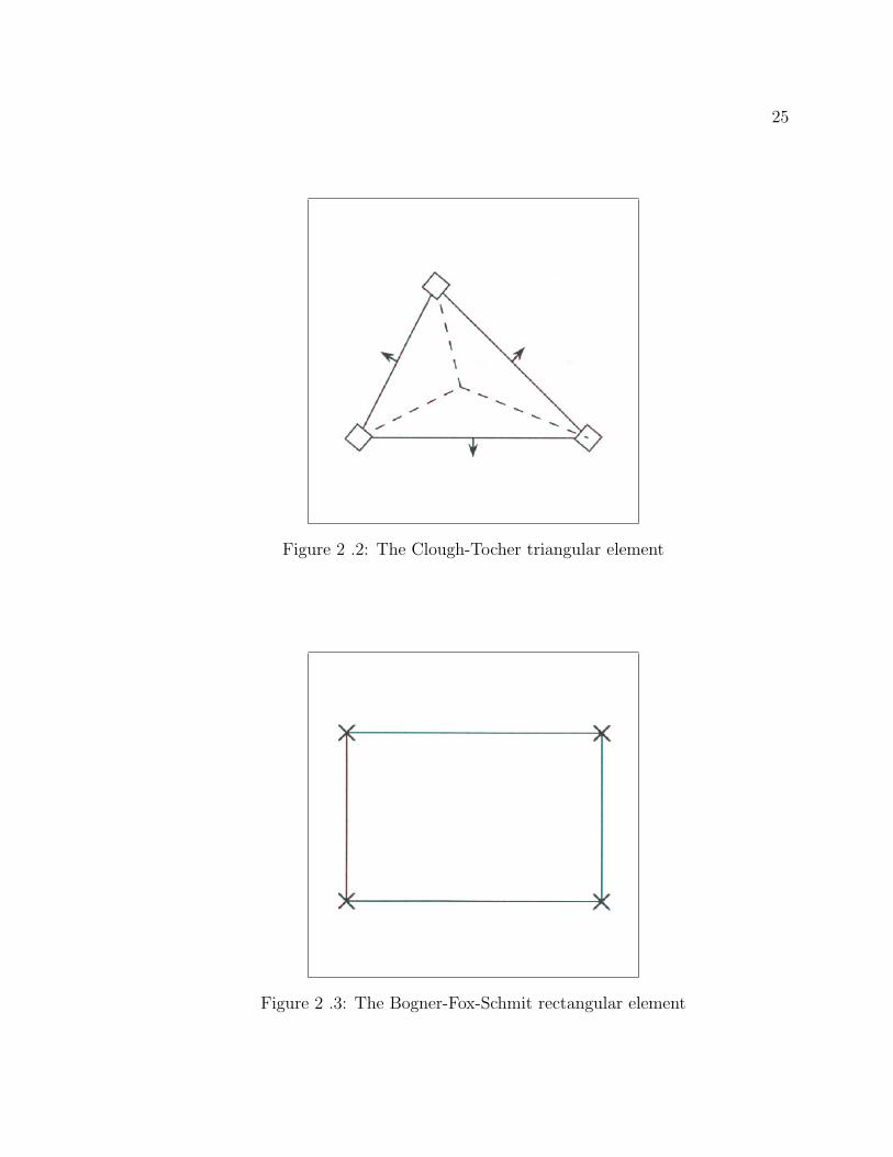
Clough-Tocher: Here we subdivide each triangle into three triangles by joining the
vertices to the centroid. In each of the smaller triangles, the functions are cubic poly-
nomials. There are then 30 degrees of freedom needed to determine the three different
24
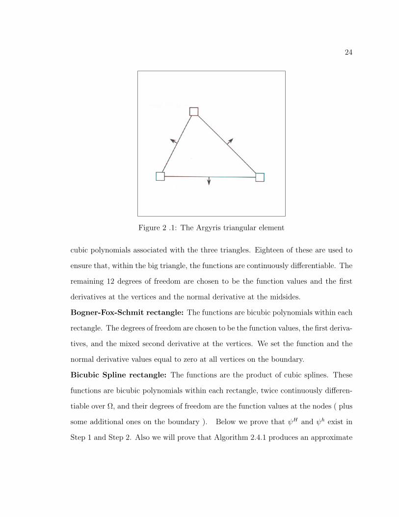
Figure 2 .1: The Argyris triangular element
cubic polynomials associated with the three triangles. Eighteen of these are used to
ensure that, within the big triangle, the functions are continuously differentiable. The
remaining 12 degrees of freedom are chosen to be the function values and the first
derivatives at the vertices and the normal derivative at the midsides.
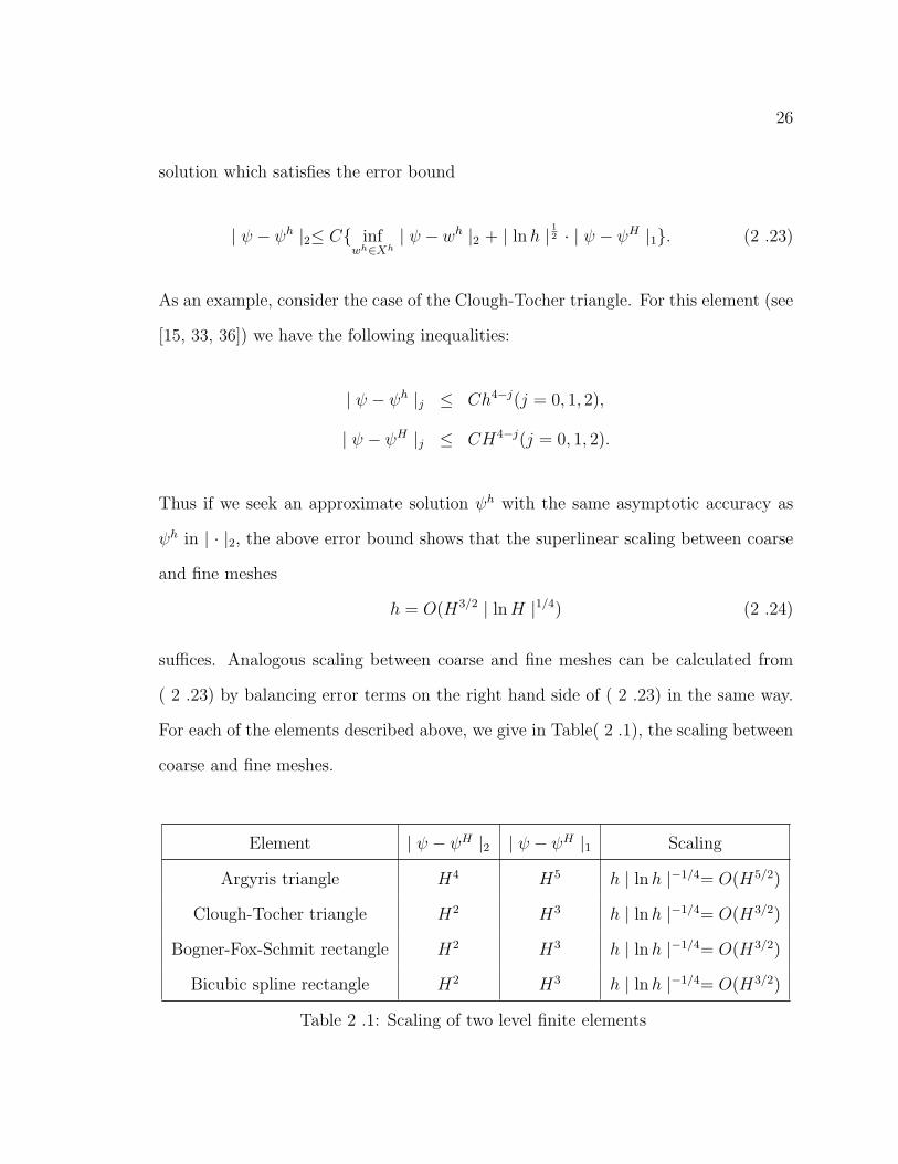
Bogner-Fox-Schmit rectangle: The functions are bicubic polynomials within each
rectangle. The degrees of freedom are chosen to be the function values, the first deriva-
tives, and the mixed second derivative at the vertices. We set the function and the
normal derivative values equal to zero at all vertices on the boundary.
Bicubic Spline rectangle: The functions are the product of cubic splines. These
functions are bicubic polynomials within each rectangle, twice continuously differen-
tiable over Ω, and their degrees of freedom are the function values at the nodes ( plus
some additional ones on the boundary ). Below we prove that ψH and ψh exist in
Step 1 and Step 2. Also we will prove that Algorithm 2.4.1 produces an approximate
25
Figure 2 .2: The Clough-Tocher triangular element
Figure 2 .3: The Bogner-Fox-Schmit rectangular element
26
solution which satisfies the error bound
| ψ − ψh |2≤ C infwh∈Xh
| ψ − wh |2 + | ln h | 12 · | ψ − ψH |1. (2 .23)
As an example, consider the case of the Clough-Tocher triangle. For this element (see
[15, 33, 36]) we have the following inequalities:
| ψ − ψh |j ≤ Ch4−j(j = 0, 1, 2),
| ψ − ψH |j ≤ CH4−j(j = 0, 1, 2).
Thus if we seek an approximate solution ψh with the same asymptotic accuracy as
ψh in | · |2, the above error bound shows that the superlinear scaling between coarse
and fine meshes
h = O(H3/2 | ln H |1/4) (2 .24)
suffices. Analogous scaling between coarse and fine meshes can be calculated from
( 2 .23) by balancing error terms on the right hand side of ( 2 .23) in the same way.
For each of the elements described above, we give in Table( 2 .1), the scaling between
coarse and fine meshes.
Element | ψ − ψH |2 | ψ − ψH |1 Scaling
Argyris triangle H4 H5 h | ln h |−1/4= O(H5/2)
Clough-Tocher triangle H2 H3 h | ln h |−1/4= O(H3/2)
Bogner-Fox-Schmit rectangle H2 H3 h | ln h |−1/4= O(H3/2)
Bicubic spline rectangle H2 H3 h | ln h |−1/4= O(H3/2)
Table 2 .1: Scaling of two level finite elements

27
2.5 The Error Bound
The basic bound on b(, , ) and b0(, , ), given in Lemma 2.3.1
| b(ψ, φ, ξ) | ≤ N | ψ |2 · | φ |2 · | ξ |2,
| b0(ψ, φ, ξ) | ≤ N | ψ |2 · | φ |2 · | ξ |2,
can be improved. For our purpose we shall be bounding | b(ψ, φ, ξ) | with φ or ξ in
a finite element space Xh or XH . Since Xh and XH are subspaces of X, then they
satisfy the following discrete Sobolev inequality: for all φh ∈ Xh (similarly for XH):
‖ 5φh ‖L∞≤ c | ln(h) |1/2| φh |2 .
Using the above inequality and Lemma 2.3.1, we can prove the following lemma:
Lemma 2.5.1
For any φh ∈ Xh, the following inequalities
| b(ψ, φh, ξ) | ≤ C | ln(h) |1/2| ψ |2 · | ξ |1 · | φh |2,
| b(ψ, ξ, φh) | ≤ C | ln(h) |1/2| ψ |2 · | ξ |1 · | φh |2
are hold.
Lemma 2.5.2
The solution to ( 2 .21) exists and satisfies | ψH |2≤ Re | f |∗. Suppose
Re2N | f |∗< 1.
Then, the solution ψH to ( 2 .21) is unique.

28
Proof: Set φH = ψH in ( 2 .21). This gives
Re−1 | ψH |22= (f, curl ψH) ≤| f |∗| ψH |2,
thus | ψH |2≤ Re | f |∗. This bound implies the existence of the solution to ( 2 .21)
by a compactness argument in XH . Let ψH1 and ψH
2 be two solutions to ( 2 .21), and
zH = ψH1 − ψH
2 . Then,
Re−1 | zH |22 = a(zH , zH) + b(ψH1 , zH , zH),
= a(ψH1 , zH) + b(ψH
1 , ψH1 , zH)− (a(ψH
2 , zH) + b(ψH1 , ψH
2 , zH)),
= b(ψH2 , ψH
2 , zH)− b(ψH1 , ψH
2 , zH),
= −b(zH , ψH2 , zH)
≤ N | zH |22| ψH2 |2≤ NRe | f |∗| zH |22,
which implies uniqueness of solutions for (1−NRe2 | f |∗) > 0, as
Re−1(1−NRe2 | f |∗) | zH |22≤ 0. ¥
The next theorem gives the basic error bound after step1 in the | · |2-seminorm.
Before we state the theorem we need the following lemma.
Lemma 2.5.3
Let ψ be a nonsingular solution of (2 .3) and provided | ψ − ψH |2≤ γ2N
, then there
is a constant γ∗ = γ∗(ψ) such that
supφ∈H2
0 (Ω)
a(ξ, φ) + b(ψH , ξ, φ) + b(ξ, ψ, φ)
| φ |2 > γ∗ | ξ |2, ∀ξ ∈ H20 (Ω). (2 .28)
29
Proof :
From (2 .20) simply follows that for | ψ−ψH |2 small enough ( which is the case with
0 < H ≤ H0 )
supφ∈H2
0 (Ω)
a(ξ, φ) + b(ψH , ξ, φ) + b(ξ, ψ, φ)
| φ |2 +b(ψ − ψH , ξ, φ)
| φ |2
≥ γ | ξ |2,∀ξ ∈ H2
0 (Ω).
But it follows from (2 .12) that
supφ∈H2
0 (Ω)
a(ξ, φ) + b(ψH , ξ, φ) + b(ξ, ψ, φ)
| φ |2 + N | ψ − ψH |2| ξ |2≥ γ | ξ |2 ∀ξ ∈ H20 (Ω),
or
supφ∈H2
0 (Ω)
a(ξ, φ) + b(ψH , ξ, φ) + b(ξ, ψ, φ)
| φ |2 ≥ (γ −N | ψ − ψH |2) | ξ |2,∀ξ ∈ H20 (Ω).
Hence, we have (2 .20). ¥
Theorem 2.5.1
(a) If the global uniqueness condition Re2N | f |∗< 1 holds,ψ and ψH both exist
uniquely. The error | ψ − ψH |2 satisfies :
| ψ − ψH |2≤ C(Re) infwH∈Xh
| ψ − wH |2,
where C(Re) = (1 + 2N | f |∗ ·Re2)(1−N | f |∗ Re2)−1 ≤ C(√
N | f |∗).(b) If the uniqueness condition fails, suppose ψ is non-singular solution of (2 .6).
Then, there is an H0 = H0(ψ, f,Re) and c = c(ψ, f,Re,N) such that for H ≤ H0,
| ψ − ψH |2≤ c(ψ, f, Re, N) infwH∈Xh
| ψ − wH |2, (2 .30)
30
where c(ψ, f, Re, N) = γ−1(Re−1 + N ·Re | f |∗) + 1
Proof:
Detailed proof of part (a) can be found in [17]. It remains to show part (b). Sub-
tracting (2 .21) from (2 .6), gives the error equation for (2 .21):
a(ψ − ψH , φH) + b(ψ, ψ, φH)− b(ψH , ψH , φH) = 0
Adding the following terms b(ψH , ψ, φH)− b(ψH , ψ, φH) gives:
a(ψ − ψH , φH) + b(ψ − ψH , ψ, φH) + b(ψH , ψ − ψH , φH) = 0
Let wh ∈ Xh be an approximation to ψ in Xh and define ξh = ψh−wh and ηh = ψ−wh
then the above inequality becomes:
a(ξH , φH) + b(ξH , ψ, φH) + b(ψH , ξH , φH) =
a(ηH , φH) + b(ηH , ψ, φH) + b(ψH , ηH , φH)
Using (2 .28) gives :
γ | ξH |2≤ supφH∈XH
| φH |−1
2
(a(ηH , φH) + b(ηH , ψ, φH) + b(ψH , ηH , φH)
)
In view of (2 .11,2 .12), we have :
| ξH |2≤ γ−1
(Re−1 + N(| ψ |2 + | ψH |2)
)| ηH |2 .
The triangle inequality (| ψ − ψh |2≤| ξh |2 + | ηh |2) implies (2 .30). ¥
31
Lemma 2.5.4
Given a solution ψH to ( 2 .21), then the solution to the following problem:
Find ψ ∈ H20 (Ω) such that , for all φ ∈ H2
0 (Ω),
a(ψ, φ) + b(ψH , ψ, φ) = l(φ)
(2 .31)
exists uniquely and satisfies: ‖ ψ ‖2≤ Re | f |∗ .
Proof:
Introducing the continuous bilinear form B : H20 (Ω)×H2
0 (Ω) → R given by
B(ψ, φ) = a(ψ, φ) + b(ψH , ψ, φ).
B is continuous and coercive. Hence, ψ exists uniquely.
Setting φ = ψ in ( 2 .31) implies that:
Re−1 ‖ ψ ‖22 = l(ψ),
‖ ψ ‖2 = Rel(ψ)
‖ ψ ‖2
,
≤ Re supφ∈H2
0 (Ω)
l(φ)
‖ φ ‖2
= Re | f |∗ . ¥
Lemma 2.5.5
Given a solution ψH to ( 2 .21), then the solution to ( 2 .22) exists uniquely and
satisfies:
‖ ψh ‖2≤ Re | f |∗ .

32
Proof:
The Bilinear form B is continuous and coercive on Xh. Hence, ψh exists uniquely.
Setting φh = ψh in ( 2 .22) implies that:
Re−1 ‖ ψh ‖22 = l(ψh),
= Rel(ψh)
‖ ψh ‖2
,
≤ Re supφ∈H2
0 (Ω)
l(φ)
‖ φ ‖2
,
= Re | f |∗ . ¥
By Green’s formula, we obtain the following lemma.
Lemma 2.5.6
For ψ, ξ, φ ∈ H20 (Ω), we have
b(ψ, ξ, φ) = b0(ξ, φ, ψ)− b0(φ, ξ, ψ). (2 .33)
Proof:
Applying Green’s formula to the left hand side of ( 2 .33) give:
b(ψ, ξ, φ) =
∫
Ω
4ψ(ξyφx − ξxφy)dΩ,
= −∫
Ω
ψx(ξyφx − ξxφy)x + ψy(ξyφx − ξxφy)y
+
∫
∂Ω
∂ψ
∂n· (ξyφx − ξxφy),

33
=
∫
Ω
(ξxxφy + ξxφyx − ξyxφx − ξyφxx)ψx
−∫
Ω
(ξyyφx + ξyφxy − ξxyφy − ξxφyy)ψy,
=
∫
Ω
(ξxyφy + ξxφyy − ξyyφx − φxyξy)ψy
−∫
Ω
(ξyφxx + φxξyx − φyξxx − ξxφyx)ψx,
=
∫
Ω
(φyξxy − φxξyy)ψy − (φxξxy − φyξxx)ψx
−∫
Ω
(ξyφxy − ξxφyy)ψy − (ξxφyx − ξyφxx)ψx,
= b0(ξ, φ, ψ)− b0(φ, ξ, ψ). ¥
The main result of this paper is the following theorem. It gives the error bound after
step2.
Theorem 2.5.2
Let Xh,H ⊂ H20 (Ω) be two finite element spaces. Let ψ be the solution to ( 2 .3) and
ψh the solution to ( 2 .22). Then ψh satisfies:
| ψ − ψh |2≤ C1 infwh∈Xh
| ψh − wh |2 +C2
√| ln h | | ψ − ψH |1,
where C1 = 2+N | f |∗ Re2 and C2 = 2N ·Re2 | f |∗ Cs, Cs is the Sobolev constant.
Proof:
Subtracting ( 2 .22) from ( 2 .3) yields:
a(ψ − ψh, φh) + b(ψ, ψ, φ)− b(ψH , ψh, φh) = 0 ∀φh ∈ Xh.

34
Using lemma 2.5.6 gives:
a(ψ − ψh, φh) + b0(ψ, φh, ψ)− b0(φh, ψ, ψ)
− b0(ψh, φh, ψH) + b0(φ
h, ψh, ψH) = 0 ∀φh ∈ Xh.
Adding the following terms:
−b0(ψh, φh, ψ) + b0(φ
h, ψh, ψ) + b0(ψh, φh, ψ)− b0(φ
h, ψh, ψ),
gives:
a(ψ − ψh, φh) + b0(ψ − ψh, φh, ψ) + b0(φh, ψh − ψ, ψ)
+ b0(ψh, φh, ψ − ψH) + b0(φ
h, ψh, ψH − ψ) = 0.
Let wh ∈ Xh be an approximation to ψ in Xh and define ξh = ψh−wh and ηh = ψ−wh,
then the above inequality becomes:
a(ηh, φh) + b0(ηh, φh, ψ)− b0(φ
h, ηh, ψ)
+ b0(ψh, φh, ψ − ψH) + b0(φ
h, ψh, ψH − ψ) =
a(ξh, φh) + b0(ξh, φh, ψ)− b0(φ
h, ξh, ψ).
Setting φh = ξh implies:
a(ξh, ξh) = a(ηh, ξh) + b0(ηh, ξh, ψ)− b0(ξ
h, ηh, ψ)
+ b0(ψh, ξh, ψ − ψH) + b0(ξ
h, ψh, ψH − ψ).

35
Using lemma 2.5.6 gives:
a(ξh, ξh) = a(ηh, ξh) + b(ψ, ηh, ξh)
+ b0(ψh, ξh, ψ − ψH) + b0(ξ
h, ψh, ψH − ψ).
We will bound the right hand side of the above inequality as follows:
a(ηh, ξh) ≤ Re−1 | ηh |2 · | ξh |2,
b(ψ, ηh, ξh) ≤ N | ψ |2 · | ηh |2 · | ξh |2,
b0(ψh, ξh, ψ − ψH) ≤ N · c | ψh |2 · | ξh |2 · | ψ − ψH |1 ·
√| ln h |,
b0(ξh, ψh, ψH − ψ) ≤ N · c | ψh |2 · | ξh |2 · | ψ − ψH |1 ·
√| ln h |.
Using these bounds gives:
Re−1 | ξh |22≤Re−1(1 + N | ψ |2 ·Re) | ηh |2 · | ξh |2+ 2Nc | ψh |2 · | ξh |2 · | ψ − ψH |1 ·
√| ln h |.
Using the bounds on | ψ |2 and | ψh |2 gives:
| ξh |2≤(1 + NRe2 | f |∗) | ηh |2+ (2NRe2 | f |∗ c)
√| ln h | | ψ − ψH |1 .
The triangle inequality (| ψ − ψh |2≤| ξh |2 + | ηh |2) implies:
| ψ − ψh |2≤(2 + NRe2 | f |∗) | ηh |2+ (2NRe2 | f |∗ c)
√| ln h | | ψ − ψH |1 .
(2 .37)

36
Hence, we have the following estimates:
| ψ − ψh |2≤ C1 infwh∈Xh
| ψ − wh |2 +C2
√| ln h |· | ψ − ψH |1 . ¥
Corollary 2.5.1
Let Xh,H be the Clough-Tocher elements. Then ψh satisfies:
| ψ − ψh |2≤ C1h2 + C2
√| ln h |H3.
2.6 Summary
Two level method for the streamfunction formulation of the Navier-Stokes equations
was discussed. The method is important because of the superlinear scaling between
the coarse and fine grids. The error between the coarse and fine meshes are related
superlinearly via:
| ψ − ψh |2≤ C infwh∈xh
| ψ − wh |2 + | ln h |1/2 · | ψ − ψH |1.
As an example, if the Clough-Tocher triangles or the Bogner-Fox-Schmit rectangles
are used, then the coarse and fine meshes are related by h = O(H3/2 | ln H |1/4).

Chapter 3
A Posteriori Error Estimator
37
38
3.1 Introduction
The use of self-adaptive mesh refinement techniques based on a posteriori error es-
timators is needed feature in any high-level finite element codes which are used for
solving a practical problem of physics or engineering such as, computational fluid
dynamics, elasticity, or semiconductor device simulation. In adaptive computation,
there is a great need of reliable error estimators for these types of practical problems.
Moreover, a priori error estimates are insufficient for mesh refinement because
they only give information on the asymptotic error behavior. Thus a posteriori error
estimators must be extracted from the computed numerical solution and the data
of the problem. The development of such estimators has been the subject of active
research over the last few years (see [66, 67] for reference). A very popular choice
for such estimators is weighted residual estimators which use some mesh-dependent
norm of the residual (see [6, 7]).
In these pages we would like to consider the application of a posteriori error anal-
ysis described in [66] to a two level finite element method for the streamfunction
formulation of the Navier-Stokes equations. We obtain a reliable posteriori error es-
timator in this problem. The attractions of the streamfunction formulation of the
Navier-Stokes equations are that the incompressibility constraint is automatically
satisfied, the pressure is not presented in the weak form and there is only one scalar
unknown to solve for. The standard weak formulation for the streamfunction version
was apparently first studied with mathematical rigor in 1979 in [33]. In this direction,
Cayco and Nicolaides [17, 16] studied a general analysis of convergence for this stan-
dard weak formulation of the Navier-Stokes equations for Reynolds numbers small
enough to ensure a global uniqueness condition holds.
The discretization of the streamfunction formulation still leads to a problem of

39
solving a large and ill-conditioned nonlinear systems of algebraic equations. two level
finite element discretization are presently a very promising approach for approxi-
mating the Navier-Stokes equations, see [41]. The computational attraction of the
methods is that they require the solution of only a small system of nonlinear equa-
tions on coarse mesh and one linear system of equations on fine mesh. These types
of methods were pioneered by Xu in [69, 70] for semilinear elliptic problems and
then analyzed for the Navier-Stokes equations using velocity-pressure formulation in
[41, 43, 44] and for the streamfunction formulation of the Navier-Stokes equations in
[26, 72].
3.2 Notations and Preliminaries
We first need to define some function spaces and associated norms. More detailed
concerning these spaces can be found in [1]. Let Ω be a bounded simply connected
polygonal domain in R2. L2(Ω) is the Hilbert space of Lebesgue square integrable
functions with norm ‖ · ‖0 and L20(Ω) is the subspace of L2(Ω) consisting of functions
with zero mean. Let Hm(Ω) be the usual Sobolev space consisting of functions which
together with their distributed derivatives up through order m are in L2(Ω). Denote
the norm on Hm(Ω) by ‖ · ‖m. Let Hm0 (Ω) be the completion of C∞
0 (Ω) under the
‖ · ‖m norm. We equip Hm0 (Ω) with the seminorm | · |m, which is a norm equivalent to
‖ · ‖m. Also, the dual of space Hm0 (Ω) is denoted by H−m(Ω), with norm ‖ · ‖−m. Let
[Hm(Ω)]2 be the space Hm(Ω)×Hm(Ω) and [Hm0 (Ω)]2 be the space Hm
0 (Ω)×Hm0 (Ω)

40
equipped with the following norm
‖ u ‖m = (‖ u1 ‖2m + ‖ u2 ‖2
m)1/2 and
| u |m = (| u1 |2m + | u2 |2m)1/2 where u =
u1
u2
.
For each φ ∈ H1(Ω), define
curl φ =
φy
−φx
.
For each u ∈ [H1(Ω)]2, define
curl u =∂u2
∂x− ∂u1
∂y, where u =
u1
u2
.
Consider the Navier-Stokes equations describing the flow of an incompressible
fluid:
−Re−1 4 u + (u · 5)u +5p = f, in Ω,
5 · u = 0, in Ω,
u = 0, on ∂Ω,∫
Ω
p dΩ = 0.
(3 .1)
Any divergence-free velocity vector u ∈ [H10 (Ω)]2 has a unique stream function [33,
Theorem3.1,page 22] ψ ∈ H20 (Ω), defined by
curl ψ = u.

41
Moreover, the streamfunction ψ satisfies
Re−1 42 ψ − ψy 4 ψx + ψx 4 ψy = curl f, in Ω,
ψ = 0, on ∂Ω,
∂ψ
∂n= 0, on ∂Ω,
(3 .3)
where n represents the outward unit normal to Ω, which is simply the curl of (‘3 .1).
The standard weak form of equation ( 3 .3) is:
Find ψ ∈ H20 (Ω) such that, for all φ ∈ H2
0 (Ω),
a(ψ, φ) + b(ψ; ψ, φ) = l(φ),
(3 .4)
where
a(ψ, φ) = Re−1
∫
Ω
4ψ · 4φ,
b(ξ; ψ, φ) =
∫
Ω
4ξ(ψyφx − ψxφy),
l(φ) = (f, curl φ) =
∫
Ω
f · curl φ.
(3 .5)
Another equivalent formulation of equation ( 3 .3), introduced by Cayco and Nico-
laides [16], is:
Find ψ ∈ H20 (Ω) such that, for all φ ∈ H2
0 (Ω),
a0(ψ, φ) + b0(ψ; ψ, φ) = l(φ),
(3 .6)

42
where
a0(ψ, φ) = Re−1
∫
Ω
ψxxφxx + 2ψxyφxy + ψyyφyy,
b0(ξ; ψ, φ) =
∫
Ω
(ξyψxy − ξxψyy)φy − (ξxψxy − ξyψxx)φx,
l(φ) = (f, curl φ) =
∫
Ω
f · curl φ.
(3 .7)
Conforming element can be used with either ( 3 .4) or ( 3 .6). In this case the
two weak formulations produce identical results because a(ψ, φ) = a0(ψ, φ) and
b(ξ; ψ, φ) = b0(ξ; ψ, φ) for all ψ, φ, ξ ∈ H20 (Ω). However, when using nonconforming
approximating subspaces, ( 3 .6) and ( 3 .4) generate different finite element methods.
Nonconforming elements should be used only with ( 3 .6). (See [16, 36] for details).
Let < ·, · > be the L2 inner product over Ω and < ·, · >e be the L2 inner product
over an element e ∈ Πh(Ω). ‖ · ‖j and ‖ · ‖j,e denote the Sobolev norm for Hj(Ω) and
Hj(e), respectively. The norm for the space X = H20 (Ω) is ‖ · ‖2. Define a nonlinear,
continuos map F : X → X ′ via the Ries representation theorem: for all ψ, φ ∈ X
< F (ψ), φ >= a(ψ, φ) + b(ψ, ψ, φ). (3 .8)
The streamfunction formulation of the Navier-Stokes equations can be represented
abstractly as:
find ψ ∈ X satisfying
< F (ψ), φ >= (f, curl φ) for all φ ∈ X. (3 .9)
Assume that the solution ψ to ( 3 .9) is nonsingular. Namely, DF (ψ) is invertable as

43
a map: X → X ′ and
‖ DF (ψ)−1 ‖L(X,X′)< ∞.
Let ΠH(Ω) and Πh(Ω), H, h > 0, be a two family of triangulations of Ω which satisfies
the following conditions:
1. any two triangles in Πh(Ω) share at most a common edge or a common vertex.
2. the minimal angle of all triangles in the whole family Πh(Ω) is bounded away
from zero.
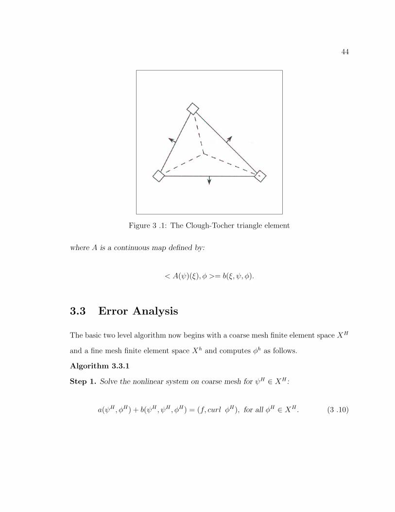
Denote by XH and Xh the spaces of Clough-Tocher elements on triangles. In
the Clough-Tocher triangle, we subdivide each triangle into three triangles by joining
the vertices to the centroid. In each of the smaller triangles, the functions are cubic
polynomials. There are then 30 degrees of freedom needed to determine the three
different cubic polynomials associated with the three triangles. Eighteen of these
these are used to ensure that, within the big triangle, the functions are continuously
differentiable. The remaining 12 degrees of freedom are chosen to be the function
values and the first derivatives at the vertices and the normal derivative at the middies.
See Figure ( 3 .1) for illustration of the Clough-Tocher triangles. The basic two level
discretization method can be written in the following algorithm.
Algorithm 3.2.1
Step 1. Calculate ψH ∈ XH by solving the (small) nonlinear system
< F (ψH), φH >= (f, curl φH), for all φH ∈ XH .
Step 2. Calculate ψh ∈ Xh by solving the linear system
< F (ψH) + A(ψH)(ψh − ψH), φh) = (f, curl φh), for all φh ∈ Xh.
44
Figure 3 .1: The Clough-Tocher triangle element
where A is a continuous map defined by:
< A(ψ)(ξ), φ >= b(ξ, ψ, φ).
3.3 Error Analysis
The basic two level algorithm now begins with a coarse mesh finite element space XH
and a fine mesh finite element space Xh and computes φh as follows.
Algorithm 3.3.1
Step 1. Solve the nonlinear system on coarse mesh for ψH ∈ XH :
a(ψH , φH) + b(ψH , ψH , φH) = (f, curl φH), for all φH ∈ XH . (3 .10)

45
Step 2. Solve the linear system on fine mesh for ψh ∈ Xh:
a(ψh, φh) + b(ψh, ψH .φh) = (f, curl φh), for allφh ∈ Xh. (3 .11)
The following relations show that the error between the coarse and fine meshes
are related superlinearly via:
| ψ − ψh |2≤ C infwh∈Xh
| ψ − wh |2 + | ln h |1/2 · | ψ − ψH |1.
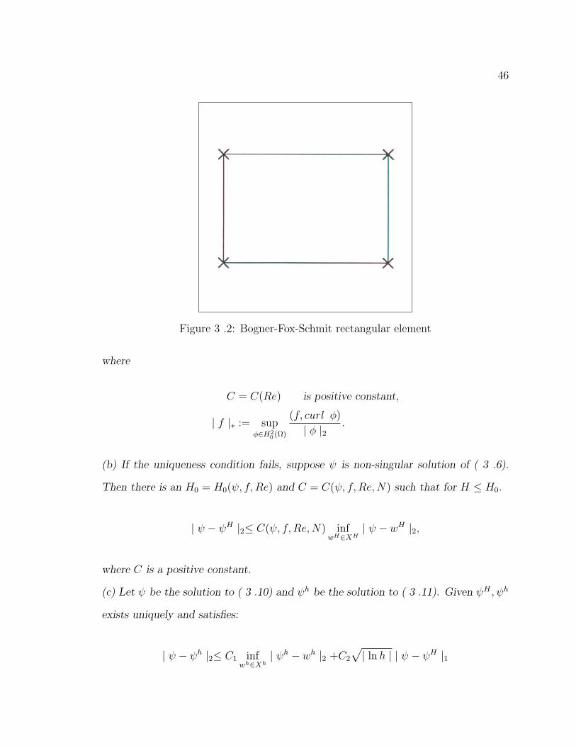
As an example, if the Bogner-Fox-Schmit rectangles, i.e the bicubic polynomials
within each rectangle whose degree of freedom are chosen to be the function val-
ues the first derivatives and the mixed second derivatives at the vertices, see Figure
( 3 .2) for illustration of the Bogner-Fox-Schmit rectangles, are used then the coarse
and fine meshes are related by
h = O(H3/2 | ln H |1/4).
The following lemma states that ψH in step 1 of Algorithm ( 3.2.1) exists uniquely
and given ψH the ψh exists uniquely under some uniqueness condition, (see [26] for
proof).
Lemma 3.3.1
(a) if the global uniqueness condition on Re2N | f |∗< 1 holds, then ψ and ψH are
both unique. The error | ψ − ψH |2 satisfies:
| ψ − ψH |2≤ C infwH∈XH
| ψ − wH |2,
46
Figure 3 .2: Bogner-Fox-Schmit rectangular element
where
C = C(Re) is positive constant,
| f |∗ := supφ∈H2
0 (Ω)
(f, curl φ)
| φ |2 .
(b) If the uniqueness condition fails, suppose ψ is non-singular solution of ( 3 .6).
Then there is an H0 = H0(ψ, f,Re) and C = C(ψ, f,Re,N) such that for H ≤ H0.
| ψ − ψH |2≤ C(ψ, f,Re, N) infwH∈XH
| ψ − wH |2,
where C is a positive constant.
(c) Let ψ be the solution to ( 3 .10) and ψh be the solution to ( 3 .11). Given ψH , ψh
exists uniquely and satisfies:
| ψ − ψh |2≤ C1 infwh∈Xh
| ψh − wh |2 +C2
√| ln h | | ψ − ψH |1
47
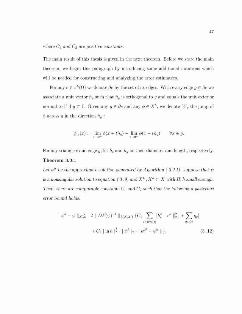
where C1 and C2 are positive constants.
The main result of this thesis is given in the next theorem. Before we state the main
theorem, we begin this paragraph by introducing some additional notations which
will be needed for constructing and analyzing the error estimators.
For any e ∈ πh(Ω) we denote ∂e by the set of its edges. With every edge g ∈ ∂e we
associate a unit vector ng such that ng is orthogonal to g and equals the unit exterior
normal to Γ if g ⊂ Γ. Given any g ∈ ∂e and any φ ∈ Xh, we denote [φ]g the jump of
φ across g in the direction ng :
[φ]g(x) := limt→0+
φ(x + tng)− limt→0+
φ(x− tng) ∀x ∈ g.
For any triangle e and edge g, let he and hg be their diameter and length, respectively.
Theorem 3.3.1
Let ψh be the approximate solution generated by Algorithm ( 3.2.1). suppose that ψ
is a nonsingular solution to equation ( 3 .9) and XH , Xh ⊂ X with H, h small enough.
Then, there are computable constants C1 and C2 such that the following a posteriori
error bound holds:
‖ ψh − ψ ‖X≤ 2 ‖ DF (ψ)−1 ‖L(X,X′) C1
∑
e∈Πh(Ω)
[h4e ‖ rh ‖2
2,e +∑
g⊂∂e
ηg]
+ C2 | ln h | 12 · | ψh |2 · | ψH − ψh |1, (3 .12)

48
where
ηg = hg ‖ Re−1[G]g ‖2L2(g) +h3
g ‖ f × ng + Re−1[54 ψh · ng]g + [F ]g · ng ‖2L2(g),
rh = curl f − [Re−1 42 ψh − ψhy 4 ψh
x + ψhx 4 ψh
y ],
F =
ψhyψh
xx − ψhxψh
xy
ψhyψh
xy − ψhxψh
yy
,
G =
5ψh
x · ng
5ψhy · ng
for any edge g.
Proof
Since ψ is a nonsingular solution, it can be shown by using the method of [33, 32]
that ψH → ψ in X as XH becomes dense in X. In particular, for H small enough
DF (ψH)−1 exists and ‖ DF (ψH)−1 ‖L(X,X′)→‖ DF (ψ)−1 ‖L(X,X′) as H → 0. Also
ψh → ψ strongly in X as H, h → 0.
Therefore, Proposition 7.1 of Verfurth [66] can be applied for H sufficiently small.
Thus, we have
‖ ψh − ψ ‖X≤ 2 ‖ DF (ψ)−1 ‖L(X,X′)‖ F (ψh)− F (ψ) ‖X′ .
The definition of the norm in X ′ gives,
‖ F (ψh)− F (ψ) ‖X′= sup0 6=φ∈X
| Q |‖ φ ‖2
,
where
Q = a(ψ, φ) + b(ψ, ψ, φ)− a(ψh, φ)− b(ψh, ψh, φ).
49
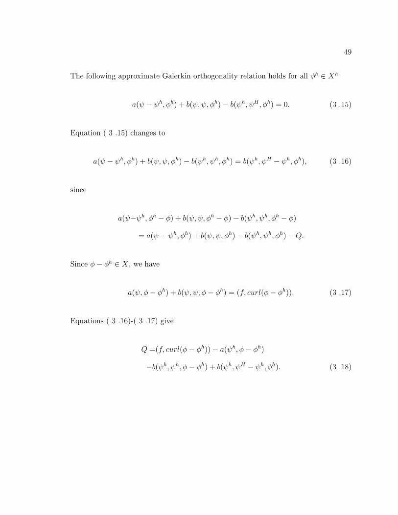
The following approximate Galerkin orthogonality relation holds for all φh ∈ Xh
a(ψ − ψh, φh) + b(ψ, ψ, φh)− b(ψh, ψH , φh) = 0. (3 .15)
Equation ( 3 .15) changes to
a(ψ − ψh, φh) + b(ψ, ψ, φh)− b(ψh, ψh, φh) = b(ψh, ψH − ψh, φh), (3 .16)
since
a(ψ−ψh, φh − φ) + b(ψ, ψ, φh − φ)− b(ψh, ψh, φh − φ)
= a(ψ − ψh, φh) + b(ψ, ψ, φh)− b(ψh, ψh, φh)−Q.
Since φ− φh ∈ X, we have
a(ψ, φ− φh) + b(ψ, ψ, φ− φh) = (f, curl(φ− φh)). (3 .17)
Equations ( 3 .16)-( 3 .17) give
Q =(f, curl(φ− φh))− a(ψh, φ− φh)
−b(ψh, ψh, φ− φh) + b(ψh, ψH − ψh, φh). (3 .18)
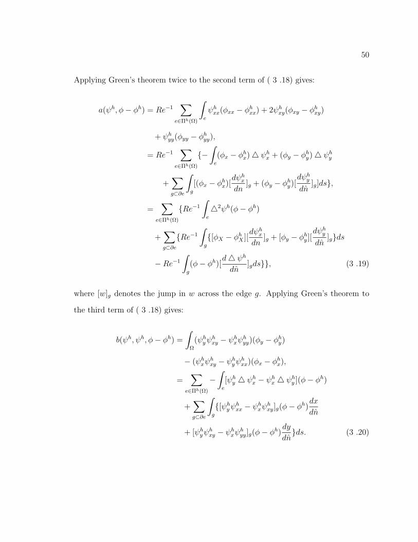
50
Applying Green’s theorem twice to the second term of ( 3 .18) gives:
a(ψh, φ− φh) = Re−1∑
e∈Πh(Ω)
∫
e
ψhxx(φxx − φh
xx) + 2ψhxy(φxy − φh
xy)
+ ψhyy(φyy − φh
yy),
= Re−1∑
e∈Πh(Ω)
−∫
e
(φx − φhx)4 ψh
x + (φy − φhy)4 ψh
y
+∑
g⊂∂e
∫
g
[(φx − φhx)[
dψhx
dn]g + (φy − φh
y)[dψh
y
dn]g]ds,
=∑
e∈Πh(Ω)
Re−1
∫
e
42ψh(φ− φh)
+∑
g⊂∂e
Re−1
∫
g
[φX − φhX ][
dψhx
dn]g + [φy − φh
y ][dψh
y
dn]gds
−Re−1
∫
g
(φ− φh)[d4 ψh
dn]gds, (3 .19)
where [w]g denotes the jump in w across the edge g. Applying Green’s theorem to
the third term of ( 3 .18) gives:
b(ψh, ψh, φ− φh) =
∫
Ω
(ψhyψh
xy − ψhxψh
yy)(φy − φhy)
− (ψhxψh
xy − ψhyψh
xx)(φx − φhx),
=∑
e∈Πh(Ω)
−∫
e
[ψhy 4 ψh
x − ψhx 4 ψh
y ](φ− φh)
+∑
g⊂∂e
∫
g
[ψhyψh
xx − ψhxψh
xy]g(φ− φh)dx
dn
+ [ψhyψh
xy − ψhxψh
yy]g(φ− φh)dy
dnds. (3 .20)
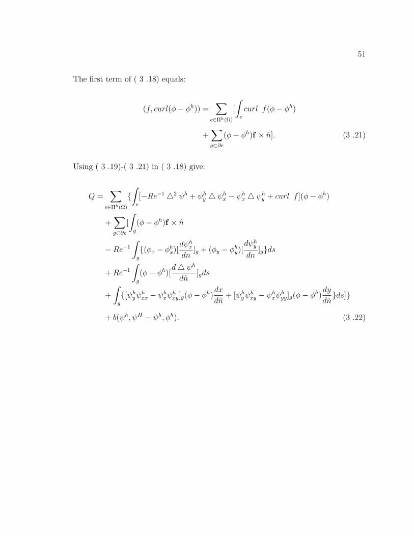
51
The first term of ( 3 .18) equals:
(f, curl(φ− φh)) =∑
e∈Πh(Ω)
[
∫
e
curl f(φ− φh)
+∑
g⊂∂e
(φ− φh)f × n]. (3 .21)
Using ( 3 .19)-( 3 .21) in ( 3 .18) give:
Q =∑
e∈Πh(Ω)
∫
e
[−Re−1 42 ψh + ψhy 4 ψh
x − ψhx 4 ψh
y + curl f ](φ− φh)
+∑
g⊂∂e
[
∫
g
(φ− φh)f × n
−Re−1
∫
g
(φx − φhx)[
dψhx
dn]g + (φy − φh
y)[dψh
y
dn]gds
+ Re−1
∫
g
(φ− φh)[d4 ψh
dn]gds
+
∫
g
[ψhyψh
xx − ψhxψh
xy]g(φ− φh)dx
dn+ [ψh
yψhxy − ψh
xψhyy]g(φ− φh)
dy
dnds]
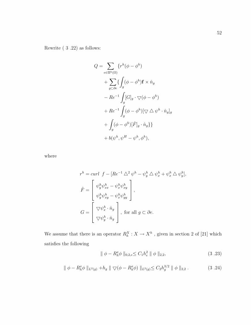
+ b(ψh, ψH − ψh, φh). (3 .22)
52
Rewrite ( 3 .22) as follows:
Q =∑
e∈Πh(Ω)
rh(φ− φh)
+∑
g⊂∂e
∫
g
(φ− φh)f × ng
−Re−1
∫
g
[G]g · 5(φ− φh)
+ Re−1
∫
g
(φ− φh)[54 ψh · ng]g
+
∫
g
(φ− φh)[F ]g · ng
+ b(ψh, ψH − ψh, φh),
where
rh = curl f − [Re−1 42 ψh − ψhy 4 ψh
x + ψhx 4 ψh
y ],
F =
ψhyψh
xx − ψhxψh
xy
ψhyψh
xy − ψhxψh
yy
,
G =
5ψh
x · ng
5ψhy · ng
, for all g ⊂ ∂e.
We assume that there is an operator RXh : X → Xh , given in section 2 of [21] which
satisfies the following
‖ φ−Rxhφ ‖0,2,e≤ C1h
2e ‖ φ ‖2,2, (3 .23)
‖ φ−Rxhφ ‖L2(g) +hg ‖ 5(φ−Rx
hφ) ‖L2(g)≤ C2h3/2g ‖ φ ‖2,2 . (3 .24)
53
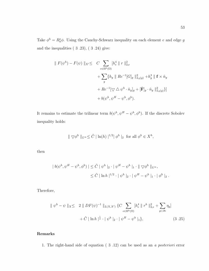
Take φh = Rxhφ. Using the Cauchy-Schwarz inequality on each element e and edge g
and the inequalities ( 3 .23), ( 3 .24) give:
‖ F (ψh)− F (ψ) ‖X′≤ C∑
e∈Πh(Ω)
[h4e ‖ r ‖2
2,e
+∑
g
hg ‖ Re−1[G]g ‖2L2(g) +h3
g ‖ f × ng
+ Re−1[54 ψh · ng]g + [F]g · ng ‖2L2(g)]
+ b(ψh, ψH − ψh, φh).
It remains to estimate the trilinear term b(ψh, ψH − ψh, φh). If the discrete Sobolev
inequality holds:
‖ 5φh ‖L∞≤ C | ln(h) |1/2| φh |2 for all φh ∈ Xh,
then
| b(ψh, ψH − ψh, φh) | ≤ C | ψh |2 · | ψH − ψh |1 · ‖ 5φh ‖L∞ ,
≤ C | ln h |1/2 · | ψh |2 · | ψH − ψh |1 · | φh |2 .
Therefore,
‖ ψh − ψ ‖X≤ 2 ‖ DF (ψ)−1 ‖L(X,X′) C∑
e∈Πh(Ω)
[h4e ‖ rh ‖2
2,e +∑
g⊂∂e
ηg]
+ C | ln h | 12 · | ψh |2 · | ψH − ψh |1, (3 .25)
Remarks
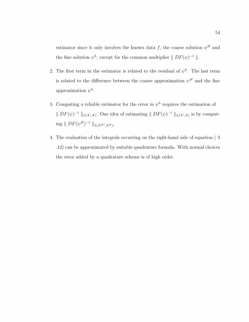
1. The right-hand side of equation ( 3 .12) can be used as an a posteriori error
54
estimator since it only involves the known data f , the coarse solution ψH and
the fine solution ψh, except for the common multiplier ‖ DF (ψ)−1 ‖.
2. The first term in the estimator is related to the residual of ψh. The last term
is related to the difference between the coarse approximation ψH and the fine
approximation ψh.
3. Computing a reliable estimator for the error in ψh requires the estimation of
‖ DF (ψ)−1 ‖L(X′,X). One idea of estimating ‖ DF (ψ)−1 ‖L(X′,X) is by comput-
ing ‖ DF (ψH)−1 ‖L(XH ′,XH).
4. The evaluation of the integrals occurring on the right-hand side of equation ( 3
.12) can be approximated by suitable quadrature formula. With normal choices
the error added by a quadrature scheme is of high order.

Chapter 4
Implementation of the Two-Level
FEM
55
56
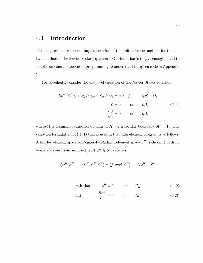
4.1 Introduction
This chapter focuses on the implementation of the finite element method for the one
level method of the Navier-Stokes equations. Our intention is to give enough detail to
enable someone competent in programming to understand the given code in Appendix
C.
For specificity, consider the one level equation of the Navier-Stokes equation.
Re−1 42 ψ + ψy 4 ψx − ψx 4 ψy = curl f, (x, y) ∈ Ω,
ψ = 0, on ∂Ω,
∂ψ
∂n= 0, on ∂Ω,
(4 .1)
where Ω is a simply connected domain in R2 with regular boundary ∂Ω = Γ. The
variation formulation of ( 4 .1) that is used in the finite element program is as follows.
A Morley element space or Bogner-Fox-Schmit element space SH is chosen ( with no
boundary conditions imposed) and ψH ∈ SH satisfies
a(ψH , φH) + b(ψH , ψH , φH) = (f, curl φH) ∀φH ∈ SH ,
such that φH = 0, on ΓH (4 .2)
and∂φH
∂n= 0 on ΓH . (4 .3)
57
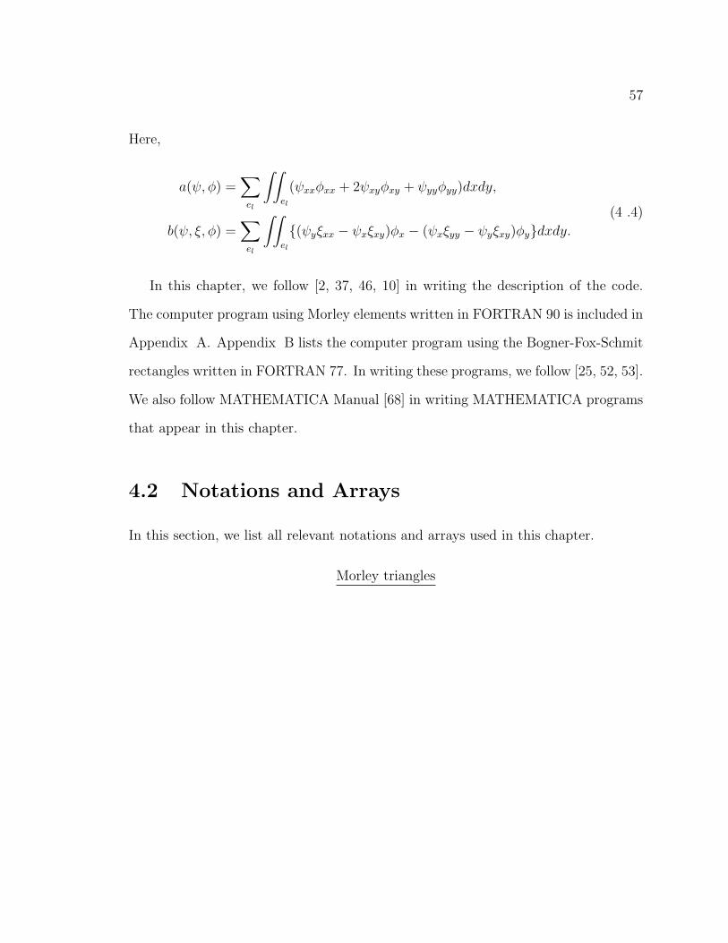
Here,
a(ψ, φ) =∑el
∫∫
el
(ψxxφxx + 2ψxyφxy + ψyyφyy)dxdy,
b(ψ, ξ, φ) =∑el
∫∫
el
(ψyξxx − ψxξxy)φx − (ψxξyy − ψyξxy)φydxdy.
(4 .4)
In this chapter, we follow [2, 37, 46, 10] in writing the description of the code.
The computer program using Morley elements written in FORTRAN 90 is included in
Appendix A. Appendix B lists the computer program using the Bogner-Fox-Schmit
rectangles written in FORTRAN 77. In writing these programs, we follow [25, 52, 53].
We also follow MATHEMATICA Manual [68] in writing MATHEMATICA programs
that appear in this chapter.
4.2 Notations and Arrays
In this section, we list all relevant notations and arrays used in this chapter.
Morley triangles
58
lx =the number of elements to be constructed
along the x-axis an the y-axis.
m =the total number of nodes on Ω ∪ Γ.
nelem =the total number of triangles in Ω.
nbf =the total number of nodes per element
nqp =the total number of integration points in the reference element.
nbo =the total number of nodes on Γ.
in = the number of nodes in Ω.
rhs(m) = the local vector.
ielnode(nelem, nbf) = global node numbers for all elements.
xx(m) = x-coordinates of all nodes.
yy(m) = y-coordinates of all nodes.
ibo(nbo) = the set of node numbers of node in Γ.
w(nqp) =the corresponding integration weights
on the reference element.
xi(nqp) =x-coordinate of the integration points
on the reference element.
eta(nqp) =y-coordinates of the integration points
on the reference element.
phi(nbf, nqp) =values of φ1, ·, φnbf at the integration points.
phix(nbf, nqp) =values of φ1,ξ, ·, φnbf,ξ at the integration points.
phiy(nbf, nqp) =values of φ1,η, ·, φnbf,η at the integration points.

59
Bogner-Fox-Schmit
lx =the number of squares along the x-axis .
m =the total number of nodes on Ω ∪ ∂Ω.
nelem =the total number of rectangles in Ω.
nbf =the total number of nodes per element
nbo =the total number of nodes on the
boundary except the y-derivative nodes on the top.
nboy =the total y-derivative nodes on the top.

60
rhs(m) = the rhs vector of the linear system.
ielnode(nelem, nbf) = global node numbers for all elements.
xx(m) = x-coordinates of all nodes.
yy(m) = y-coordinates of all nodes.
ibo(nbo) = the set of node numbers of nodes in
∂Ω except the y-derivative nodes on the top.
iboy(nboy) = the set of node numbers of y-derivative node on the top.
xi(4) = x-coordinate of integration points on the reference.
eta(4) = y-coordinate of integration points on the reference.
w(4) = the corresponding integration weights
on the reference element.
q(nbf, 6, 4) = the basis function values, x-derivative,
y-derivative, xy-derivative, xx-derivative
and yy-derivative of all 16 basis functions
at the integration points.
ea(i, j) =
∫∫
e
(φi,xxφj,xx + 2φi,xyφj,xy + φi,yyφj,yy)dξdη.
b(i, j, k) =
∫∫
e
(φj,yφk,xx − φj,xφk,xy)φi,x
− (φj,xφk,yy − φj,yφk,xy)φi,ydξdη.
4.3 Mesh Generation
SUBROUTINE MAELNODE generates the data points associated with a regular
triangle mesh on the unit square [0, 1]× [0, 1]. The number of triangular elements to
be placed along each axis is determined by lx. Since there must be an even number

61
Figure 4 .1: Triangles labeling
of elements on each level, then m is always an even number. A crude diagram of the
subject mesh is presented in Figure ( 4 .1) for case lx = 3. the triangles are labeled in
increasing order from bottom left corner to the top right corner. The number of nodes
per element is set by nbf = 6. In Morley element form, MAELNODE places nodes
at the vertices and at the midpoints of each edge. The nodes are labeled globally in
increasing order from bottom left corner to the top right corner as shown in Figure
( 4 .2). These nodes are numbered globally and their x− y coordinates are computed
by the SUBROUTINE COORD(....) and stored in the real array x(:) and y(:). For
the midside nodes, we have to store the information of the direction of the normal.
Thus information will be described in the next paragraph.
In addition, it is necessary to have a local node ordering. An example of a local node
ordering on a triangle is shown in Figure ( 4 .3). By convention, we order the nodes
counter clockwise beginning with the vertex nodes, then the edge nodes. For the
midside nodes, we assign a positive value if the arrow is outward with respect to the
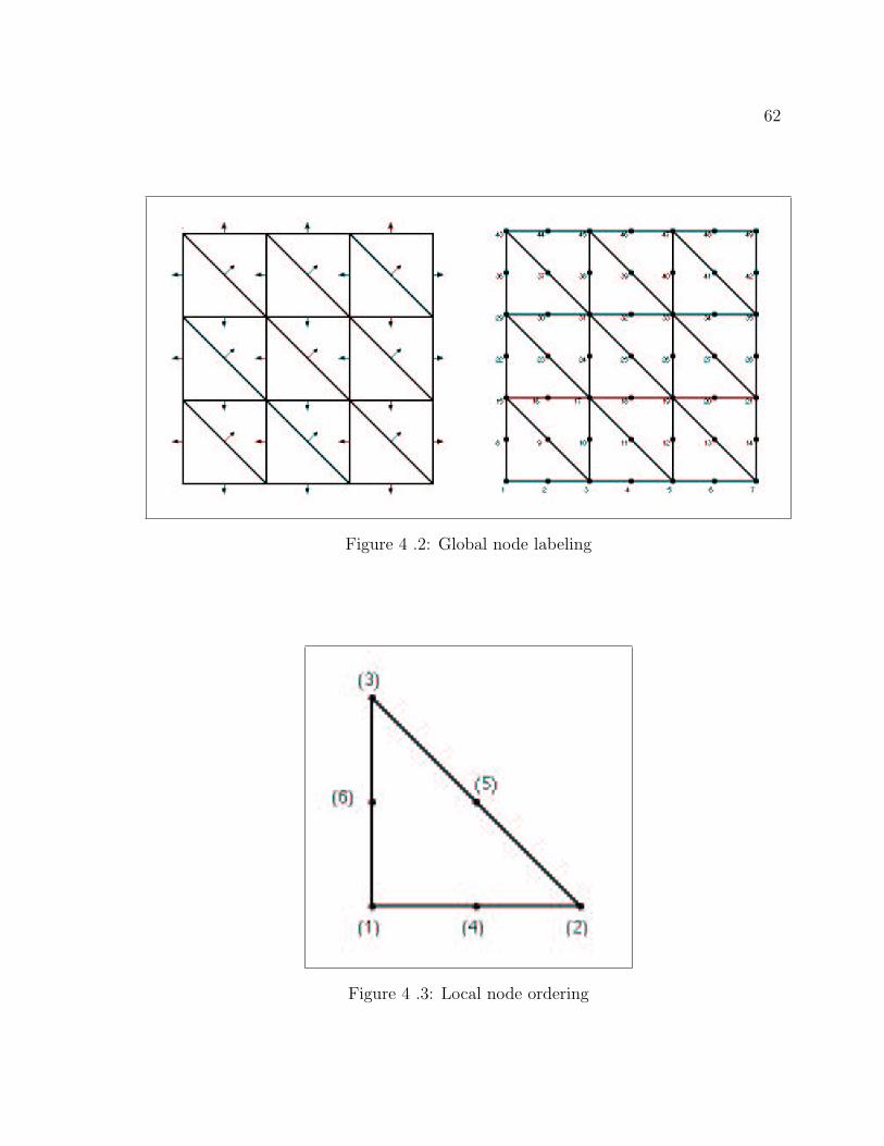
62
Figure 4 .2: Global node labeling
Figure 4 .3: Local node ordering

63
given triangle and negative value if it is inward.
This local ordering is stored in an array ielnode(nelem × nbf) where nelem = lx2,
nbf = 6. Specifically,
ielnode(i, j) := the global node number of node j in triangle i,
i = 1, 2, . . . . . . , nbf = 6,
j = 1, 2, . . . . . . , nelem = 2 ∗ lx2.
For example, the coordinates of the third node in the fifth triangle are
x = x(ielnode(3, 5)), y = y(ielnode(3, 5)).
Moreover, the boundary nodes are stored in the array ibo. The number of boundary
nodes nbo for a unit square is given by the following relation nbo = 8∗ lx. An example
of ielnode array of Figure ( 4 .2) are given below. An example of a local vs. global
node ordering for element e3 in Figure ( 4 .1) is given in the third row of ielnode
array (i.e) (3, 5, 17, 4, 11, 10). Notice that the last three columns in ielnode have
some negative values. These last three columns represent the midsides points of each
triangles. There negative values say that the arrow is inward. Moreover, the negative
values appear only on the even rows because only the triangle given even number has

64
inward arrow.
ielnode =
1 3 15 2 9 8
17 15 3 −16 −9 −10
3 5 17 4 11 10
19 17 5 −18 −11 −12
5 7 19 6 13 12
21 19 7 −20 −13 14
15 17 29 16 23 22
31 29 17 −30 −23 −24
17 19 31 18 25 24
33 31 19 −32 −25 −26
19 21 33 20 27 26
35 33 21 34 −27 28
29 31 43 30 37 36
45 43 31 −44 −37 −38
31 33 45 32 39 38
47 45 33 46 −39 −40
33 35 47 34 41 40
49 47 35 48 −41 42
An example of x, y and ibo arrays of Figure ( 4 .2) are given below. An example
of x-coordinate and y-coordinate of the node 25 is (0.5,0.5) which is 25-th entry in
x-array and y-array. Also, ibo-array lists all the boundary node numbers of Figure
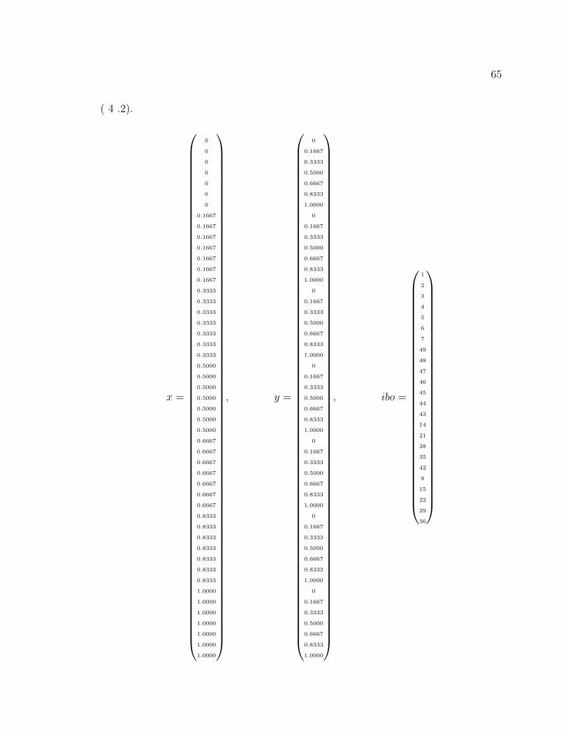
65
( 4 .2).
x =
0
0
0
0
0
0
0
0.1667
0.1667
0.1667
0.1667
0.1667
0.1667
0.1667
0.3333
0.3333
0.3333
0.3333
0.3333
0.3333
0.3333
0.5000
0.5000
0.5000
0.5000
0.5000
0.5000
0.5000
0.6667
0.6667
0.6667
0.6667
0.6667
0.6667
0.6667
0.8333
0.8333
0.8333
0.8333
0.8333
0.8333
0.8333
1.0000
1.0000
1.0000
1.0000
1.0000
1.0000
1.0000
, y =
0
0.1667
0.3333
0.5000
0.6667
0.8333
1.0000
0
0.1667
0.3333
0.5000
0.6667
0.8333
1.0000
0
0.1667
0.3333
0.5000
0.6667
0.8333
1.0000
0
0.1667
0.3333
0.5000
0.6667
0.8333
1.0000
0
0.1667
0.3333
0.5000
0.6667
0.8333
1.0000
0
0.1667
0.3333
0.5000
0.6667
0.8333
1.0000
0
0.1667
0.3333
0.5000
0.6667
0.8333
1.0000
, ibo =
1
2
3
4
5
6
7
49
48
47
46
45
44
43
14
21
28
35
42
8
15
22
29
36
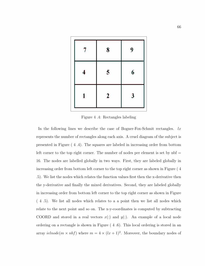
66
Figure 4 .4: Rectangles labeling
In the following lines we describe the case of Bogner-Fox-Schmit rectangles. lx
represents the number of rectangles along each axis. A cruel diagram of the subject is
presented in Figure ( 4 .4). The squares are labeled in increasing order from bottom
left corner to the top right corner. The number of nodes per element is set by nbf =
16. The nodes are labelled globally in two ways. First, they are labeled globally in
increasing order from bottom left corner to the top right corner as shown in Figure ( 4
.5). We list the nodes which relates the function values first then the x-derivative then
the y-derivative and finally the mixed derivatives. Second, they are labeled globally
in increasing order from bottom left corner to the top right corner as shown in Figure
( 4 .5). We list all nodes which relates to a a point then we list all nodes which
relate to the next point and so on. The x-y-coordinates is computed by subtracting
COORD and stored in a real vectors x(:) and y(:). An example of a local node
ordering on a rectangle is shown in Figure ( 4 .6). This local ordering is stored in an
array ielnode(m × nbf) where m = 4 × (lx + 1)2. Moreover, the boundary nodes of

67
Figure 4 .5: Global node ordering
the top are stored in iboy and the others are stored in ibo.
4.4 Affine Mapping
After we compute the ielnode array and the x-coordinate and y-coordinate for each
point, each triangle element is then the image of a reference element under an affine
transformation. Let e denote the reference triangle in the parameter space with
vertices (0.0). (1,0) and (0,1) as shown in Figure ( 4 .7). The vertex nodes of e are
ordered, as indicated, counterclockwise beginning with (0,0). The vertex nodes of the
l-th element el in ΩH are then found by searching through the arrays ielnode, xx and
yy:
k1 = ielnode(l, 1),
k2 = ielnode(l, 2),
k3 = ielnode(l, 3),
(4 .5)

68
Figure 4 .6: Local node ordering
Figure 4 .7: The reference Triangle

69
given the global node number of the three vertex nodes. Their coordinates are then
xk1 = xx(k1), yk1 = yy(k1),
xk2 = xx(k2), yk2 = yy(k2),
xk3 = xx(k3), yk3 = yy(k3).
(4 .6)
The affine map formed using these coordinates
x
y
= F2×2
ξ
η
+
b1
b2
, (4 .7)
where specifically,
x = [xk2 − xk1] ξ + [xk3 − xk1] η + xk1,
y = [yk2 − yk1] ξ + [yk3 − yk1] η + yk1,
(4 .8)
then maps e to el. The affine map for mesh shown in Figure ( 4 .7) is
x = [xk2 − xk1] ξ + xk1,
y = [yk3 − yk1] η + yk1.
(4 .9)
In addition, it maps node (1) in e to node(1) (with coordinates (xk1, yk1)) in el, node(2)
in e to node(2) in el, and node(3) in e to node(3) in el. Further, edge midpoints are
mapped to corresponding edge midpoints.
In rectangle element, let e denote the reference rectangle in the parameter space
with vertices (-1,1), (1,-1), (-1,1) and (1,1) as shown in Figure ( 4 .8). The affine map

70
Figure 4 .8: The reference rectangle
is
x =h
2(ξ − 1) + x2,
y =h
2(η − 1) + y3,
(4 .10)
where
xi = x(ielnode(l, i)),
yi = y(ielnode(l, i)),
h = x2 − x1 = y3 − y1.

71
4.5 Basis Functions for Morley Element
Now, consider the construction of quadratic basis functions on the reference trian-
gle with vertices (0,0), (1,0) and(0,1), given the reference nodes N1 = (0, 0), N2 =
(1, 0), N3 = (0, 1), N4 = (1/2, 0), N5 = (1/2, 1/2) and N6 = (0, 1/2). On the reference
element the basis function is of the form
φ(ξ, η) = c1ξ2 + c2η
2 + c3ξη + c4ξ + c5η + c6,
and thus the values of φ is specified at the three vertex nodes and ∂φ∂n
is specified at
the three mid-side point nodes. Here, φ1 has to satisfy
φ1(N1) = 1, −∂φ1
∂y(N4) = 0, (4 .11)
φ1(N2) = 0,1√2(∂φ1
∂ξ(N5) +
∂φ1
∂y(N5)) = 0, (4 .12)
φ1(N3) = 0,∂φ1
∂ξ(N6) = 0. (4 .13)
Also, φ5 has to satisfy
φ5(N1) = 0, −∂φ5
∂η(N4) = 0, (4 .14)
φ5(N2) = 0,1√2(∂φ1
∂ξ(N5) +
∂φ5
∂η(N5)) = 1, (4 .15)
φ5(N3) = 0,∂φ5
∂ξ(N6) = 0. (4 .16)
The coefficients of the basis function φi can be precomputed with MATHEMAT-
ICA
f[x_,y_]:=f1 x^2+f2 y^2+f3 x y+f4 x+f5 y+f6
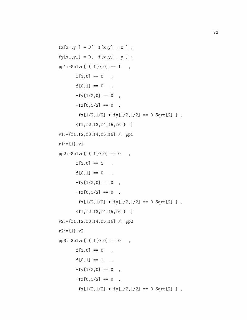
72
fx[x_,y_] = D[ f[x,y] , x ] ;
fy[x_,y_] = D[ f[x,y] , y ] ;
pp1:=Solve[ f[0,0] == 1 ,
f[1,0] == 0 ,
f[0,1] == 0 ,
-fy[1/2,0] == 0 ,
-fx[0,1/2] == 0 ,
fx[1/2,1/2] + fy[1/2,1/2] == 0 Sqrt[2] ,
f1,f2,f3,f4,f5,f6 ]
v1:=f1,f2,f3,f4,f5,f6 /. pp1
r1:=1.v1
pp2:=Solve[ f[0,0] == 0 ,
f[1,0] == 1 ,
f[0,1] == 0 ,
-fy[1/2,0] == 0 ,
-fx[0,1/2] == 0 ,
fx[1/2,1/2] + fy[1/2,1/2] == 0 Sqrt[2] ,
f1,f2,f3,f4,f5,f6 ]
v2:=f1,f2,f3,f4,f5,f6 /. pp2
r2:=1.v2
pp3:=Solve[ f[0,0] == 0 ,
f[1,0] == 0 ,
f[0,1] == 1 ,
-fy[1/2,0] == 0 ,
-fx[0,1/2] == 0 ,
fx[1/2,1/2] + fy[1/2,1/2] == 0 Sqrt[2] ,
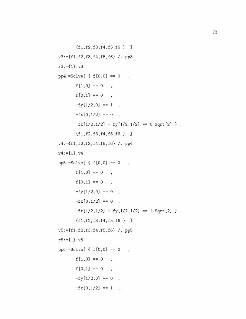
73
f1,f2,f3,f4,f5,f6 ]
v3:=f1,f2,f3,f4,f5,f6 /. pp3
r3:=1.v3
pp4:=Solve[ f[0,0] == 0 ,
f[1,0] == 0 ,
f[0,1] == 0 ,
-fy[1/2,0] == 1 ,
-fx[0,1/2] == 0 ,
fx[1/2,1/2] + fy[1/2,1/2] == 0 Sqrt[2] ,
f1,f2,f3,f4,f5,f6 ]
v4:=f1,f2,f3,f4,f5,f6 /. pp4
r4:=1.v4
pp5:=Solve[ f[0,0] == 0 ,
f[1,0] == 0 ,
f[0,1] == 0 ,
-fy[1/2,0] == 0 ,
-fx[0,1/2] == 0 ,
fx[1/2,1/2] + fy[1/2,1/2] == 1 Sqrt[2] ,
f1,f2,f3,f4,f5,f6 ]
v5:=f1,f2,f3,f4,f5,f6 /. pp5
r5:=1.v5
pp6:=Solve[ f[0,0] == 0 ,
f[1,0] == 0 ,
f[0,1] == 0 ,
-fy[1/2,0] == 0 ,
-fx[0,1/2] == 1 ,

74
fx[1/2,1/2] + fy[1/2,1/2] == 0 Sqrt[2] ,
f1,f2,f3,f4,f5,f6 ]
v6:=f1,f2,f3,f4,f5,f6 /. pp6
r6:=1.v6
a = r1,r2,r3,r4,r5,r6
The basis functions are given explicitly by
φ1(ξ, η) = 1− ξ − η + 2ξη,
φ2(ξ, η) = ξ/2 + ξ2/2 + η/2− ξη − η2/2,
φ3(ξ, η) = ξ/2− ξ2/2 + η/2− ξη + η2/2,
φ4(ξ, η) = −η + η2,
φ5(ξ, η) = −ξ + ξ2 − η + 2ξη + η2/√
2,
φ6(ξ, η) = −ξ + ξ2.
(4 .17)
The local basis functions on el are simply the image of these under the affine map
( 4 .9). For example, the local basis functions associated with the node Ni has the
following graph. Figure ( 4 .9) shows the graph of three basis functions. These local
basis functions on adjacent triangles are combined to form a global basis functions
that is continuous at the vertices of each triangle and the normal derivatives are
continuous at the mid-sides. Associated with vertex node Ni in ΩH is the global basis
function that has values 1 at Ni and zero at the remaining vertex nodes and zero
normal derivatives at all midside point nodes. Associated with midside nodes Nj in
ΩH is a global basis function that has normal derivative 1 at Nj and zero at all the
remaining midside nodes and zero function value at all vertex nodes.
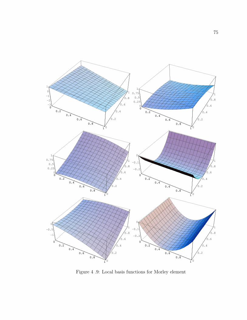
75
00.2
0.4
0.6
0.8
1 0
0.2
0.4
0.6
0.8
1
-3
-2
-1
0
1
00.2
0.4
0.6
0.8
1
00.2
0.4
0.6
0.8
1 0
0.2
0.4
0.6
0.8
1
0
0.25
0.5
0.75
1
00.2
0.4
0.6
0.8
1
00.2
0.4
0.6
0.8
1 0
0.2
0.4
0.6
0.8
1
0
0.25
0.5
0.75
1
00.2
0.4
0.6
0.8
1
00.2
0.4
0.6
0.8
1 0
0.2
0.4
0.6
0.8
1
-0.2
-0.1
0
00.2
0.4
0.6
0.8
1
00.2
0.4
0.6
0.8
1 0
0.2
0.4
0.6
0.8
1
-1
-0.5
0
00.2
0.4
0.6
0.8
1
00.2
0.4
0.6
0.8
1 0
0.2
0.4
0.6
0.8
1
-0.2
-0.1
0
00.2
0.4
0.6
0.8
1
Figure 4 .9: Local basis functions for Morley element
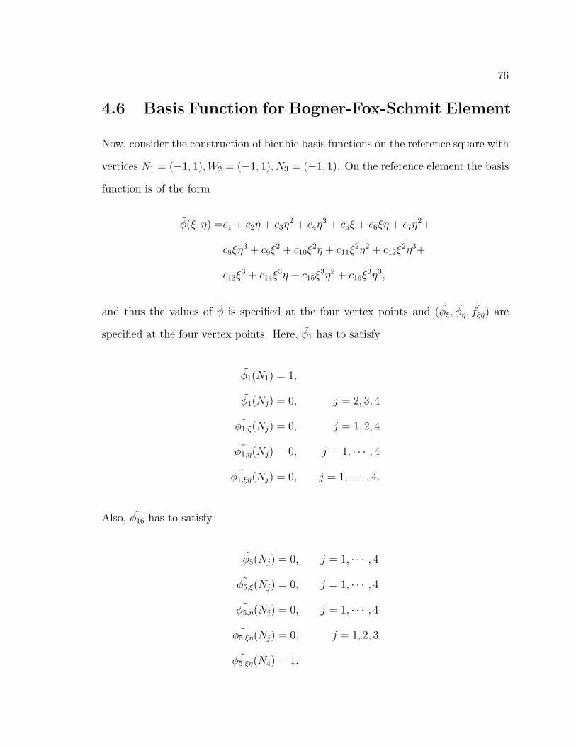
76
4.6 Basis Function for Bogner-Fox-Schmit Element
Now, consider the construction of bicubic basis functions on the reference square with
vertices N1 = (−1, 1),W2 = (−1, 1), N3 = (−1, 1). On the reference element the basis
function is of the form
φ(ξ, η) =c1 + c2η + c3η2 + c4η
3 + c5ξ + c6ξη + c7η2+
c8ξη3 + c9ξ
2 + c10ξ2η + c11ξ
2η2 + c12ξ2η3+
c13ξ3 + c14ξ
3η + c15ξ3η2 + c16ξ
3η3,
and thus the values of φ is specified at the four vertex points and (φξ, φη, fξη) are
specified at the four vertex points. Here, φ1 has to satisfy
φ1(N1) = 1,
φ1(Nj) = 0, j = 2, 3, 4
˜φ1,ξ(Nj) = 0, j = 1, 2, 4
˜φ1,η(Nj) = 0, j = 1, · · · , 4
˜φ1,ξη(Nj) = 0, j = 1, · · · , 4.
Also, φ16 has to satisfy
φ5(Nj) = 0, j = 1, · · · , 4
˜φ5,ξ(Nj) = 0, j = 1, · · · , 4
˜φ5,η(Nj) = 0, j = 1, · · · , 4
˜φ5,ξη(Nj) = 0, j = 1, 2, 3
˜φ5,ξη(N4) = 1.

77
The coefficients of the basis function φi can be precomputed with MATHEMATICA
vv = 1,y,y^2,y^3,x,x y,x y^2,x y^3,
x^2,x^2 y,x^2 y^2,x^2 y^3,
x^3,x^3 y,x^3 y^2,x^3 y^3;
vc=f1,f2,f3,f4,f5,f6,f7,f8,f9,f10,f11,
f12,f13,f14,f15,f16;
f[x_,y_]=vv.vc;
fx[x_,y_] = D[ f[x,y] , x ] ;
fy[x_,y_] = D[ f[x,y] , y ] ;
fxy[x_,y_] = D[ fx[x,y] , y ] ;
pp1:=Solve[
f[-1,-1] == 1, fx[-1,-1] == 0, fy[-1,-1] == 0, fxy[-1,-1] == 0,
f[1,-1] == 0, fx[1,-1] == 0, fy[1,-1] == 0, fxy[1,-1] == 0,
f[-1,1] == 0, fx[-1,1] == 0, fy[-1,1] == 0, fxy[-1,1] == 0,
f[1,1] == 0, fx[1,1] == 0, fy[1,1] == 0, fxy[1,1] == 0
,
f1,f2,f3,f4,f5,f6,f7,f8,f9,f10,f11,
f12,f13,f14,f15,f16 ]
v1:=f1,f2,f3,f4,f5,f6,f7,f8,f9,f10,f11,
f12,f13,f14,f15,f16 /. pp1
r1:=1.v1
pp2:=Solve[
f[-1,-1] == 0, fx[-1,-1] == 0, fy[-1,-1] == 0, fxy[-1,-1] == 0,
f[1,-1] == 1, fx[1,-1] == 0, fy[1,-1] == 0, fxy[1,-1] == 0,
f[-1,1] == 0, fx[-1,1] == 0, fy[-1,1] == 0, fxy[-1,1] == 0,
78
f[1,1] == 0, fx[1,1] == 0, fy[1,1] == 0, fxy[1,1] == 0
,
f1,f2,f3,f4,f5,f6,f7,f8,f9,f10,f11,
f12,f13,f14,f15,f16 ]
v2:=f1,f2,f3,f4,f5,f6,f7,f8,f9,f10,f11,
f12,f13,f14,f15,f16 /. pp2
r2:=1.v2
pp3:=Solve[
f[-1,-1] == 0, fx[-1,-1] == 0, fy[-1,-1] == 0, fxy[-1,-1] == 0,
f[1,-1] == 0, fx[1,-1] == 0, fy[1,-1] == 0, fxy[1,-1] == 0,
f[-1,1] == 1, fx[-1,1] == 0, fy[-1,1] == 0, fxy[-1,1] == 0,
f[1,1] == 0, fx[1,1] == 0, fy[1,1] == 0, fxy[1,1] == 0
,
f1,f2,f3,f4,f5,f6,f7,f8,f9,f10,f11,
f12,f13,f14,f15,f16 ]
v3:=f1,f2,f3,f4,f5,f6,f7,f8,f9,f10,f11,
f12,f13,f14,f15,f16 /. pp3
r3:=1.v3
pp4:=Solve[
f[-1,-1] == 0, fx[-1,-1] == 0, fy[-1,-1] == 0, fxy[-1,-1] == 0,
f[1,-1] == 0, fx[1,-1] == 0, fy[1,-1] == 0, fxy[1,-1] == 0,
f[-1,1] == 0, fx[-1,1] == 0, fy[-1,1] == 0, fxy[-1,1] == 0,
f[1,1] == 1, fx[1,1] == 0, fy[1,1] == 0, fxy[1,1] == 0
,
f1,f2,f3,f4,f5,f6,f7,f8,f9,f10,f11,
f12,f13,f14,f15,f16 ]
79
v4:=f1,f2,f3,f4,f5,f6,f7,f8,f9,f10,f11,
f12,f13,f14,f15,f16 /. pp4
r4:=1.v4
pp5:=Solve[
f[-1,-1] == 0, fx[-1,-1] == 1, fy[-1,-1] == 0, fxy[-1,-1] == 0,
f[1,-1] == 0, fx[1,-1] == 0, fy[1,-1] == 0, fxy[1,-1] == 0,
f[-1,1] == 0, fx[-1,1] == 0, fy[-1,1] == 0, fxy[-1,1] == 0,
f[1,1] == 0, fx[1,1] == 0, fy[1,1] == 0, fxy[1,1] == 0
,
f1,f2,f3,f4,f5,f6,f7,f8,f9,f10,f11,
f12,f13,f14,f15,f16 ]
v5:=f1,f2,f3,f4,f5,f6,f7,f8,f9,f10,f11,
f12,f13,f14,f15,f16 /. pp5
r5:=1.v5
pp6:=Solve[
f[-1,-1] == 0, fx[-1,-1] == 0, fy[-1,-1] == 0, fxy[-1,-1] == 0,
f[1,-1] == 0, fx[1,-1] == 1, fy[1,-1] == 0, fxy[1,-1] == 0,
f[-1,1] == 0, fx[-1,1] == 0, fy[-1,1] == 0, fxy[-1,1] == 0,
f[1,1] == 0, fx[1,1] == 0, fy[1,1] == 0, fxy[1,1] == 0
,
f1,f2,f3,f4,f5,f6,f7,f8,f9,f10,f11,
f12,f13,f14,f15,f16 ]
v6:=f1,f2,f3,f4,f5,f6,f7,f8,f9,f10,f11,
f12,f13,f14,f15,f16 /. pp6
r6:=1.v6
pp7:=Solve[

80
f[-1,-1] == 0, fx[-1,-1] == 0, fy[-1,-1] == 0, fxy[-1,-1] == 0,
f[1,-1] == 0, fx[1,-1] == 0, fy[1,-1] == 0, fxy[1,-1] == 0,
f[-1,1] == 0, fx[-1,1] == 1, fy[-1,1] == 0, fxy[-1,1] == 0,
f[1,1] == 0, fx[1,1] == 0, fy[1,1] == 0, fxy[1,1] == 0
,
f1,f2,f3,f4,f5,f6,f7,f8,f9,f10,f11,
f12,f13,f14,f15,f16 ]
v7:=f1,f2,f3,f4,f5,f6,f7,f8,f9,f10,f11,
f12,f13,f14,f15,f16 /. pp7
r7:=1.v7
pp8:=Solve[
f[-1,-1] == 0, fx[-1,-1] == 0, fy[-1,-1] == 0, fxy[-1,-1] == 0,
f[1,-1] == 0, fx[1,-1] == 0, fy[1,-1] == 0, fxy[1,-1] == 0,
f[-1,1] == 0, fx[-1,1] == 0, fy[-1,1] == 0, fxy[-1,1] == 0,
f[1,1] == 0, fx[1,1] == 1, fy[1,1] == 0, fxy[1,1] == 0
,
f1,f2,f3,f4,f5,f6,f7,f8,f9,f10,f11,
f12,f13,f14,f15,f16 ]
v8:=f1,f2,f3,f4,f5,f6,f7,f8,f9,f10,f11,
f12,f13,f14,f15,f16 /. pp8
r8:=1.v8
pp9:=Solve[
f[-1,-1] == 0, fx[-1,-1] == 0, fy[-1,-1] == 1, fxy[-1,-1] == 0,
f[1,-1] == 0, fx[1,-1] == 0, fy[1,-1] == 0, fxy[1,-1] == 0,
f[-1,1] == 0, fx[-1,1] == 0, fy[-1,1] == 0, fxy[-1,1] == 0,
f[1,1] == 0, fx[1,1] == 0, fy[1,1] == 0, fxy[1,1] == 0

81
,
f1,f2,f3,f4,f5,f6,f7,f8,f9,f10,f11,
f12,f13,f14,f15,f16 ]
v9:=f1,f2,f3,f4,f5,f6,f7,f8,f9,f10,f11,
f12,f13,f14,f15,f16 /. pp9
r9:=1.v9
pp10:=Solve[
f[-1,-1] == 0, fx[-1,-1] == 0, fy[-1,-1] == 0, fxy[-1,-1] == 0,
f[1,-1] == 0, fx[1,-1] == 0, fy[1,-1] == 1, fxy[1,-1] == 0,
f[-1,1] == 0, fx[-1,1] == 0, fy[-1,1] == 0, fxy[-1,1] == 0,
f[1,1] == 0, fx[1,1] == 0, fy[1,1] == 0, fxy[1,1] == 0
,
f1,f2,f3,f4,f5,f6,f7,f8,f9,f10,f11,
f12,f13,f14,f15,f16 ]
v10:=f1,f2,f3,f4,f5,f6,f7,f8,f9,f10,f11,
f12,f13,f14,f15,f16 /. pp10
r10:=1.v10
pp11:=Solve[
f[-1,-1] == 0, fx[-1,-1] == 0, fy[-1,-1] == 0, fxy[-1,-1] == 0,
f[1,-1] == 0, fx[1,-1] == 0, fy[1,-1] == 0, fxy[1,-1] == 0,
f[-1,1] == 0, fx[-1,1] == 0, fy[-1,1] == 1, fxy[-1,1] == 0,
f[1,1] == 0, fx[1,1] == 0, fy[1,1] == 0, fxy[1,1] == 0
,
f1,f2,f3,f4,f5,f6,f7,f8,f9,f10,f11,
f12,f13,f14,f15,f16 ]
v11:=f1,f2,f3,f4,f5,f6,f7,f8,f9,f10,f11,

82
f12,f13,f14,f15,f16 /. pp11
r11:=1.v11
pp12:=Solve[
f[-1,-1] == 0, fx[-1,-1] == 0, fy[-1,-1] == 0, fxy[-1,-1] == 0,
f[1,-1] == 0, fx[1,-1] == 0, fy[1,-1] == 0, fxy[1,-1] == 0,
f[-1,1] == 0, fx[-1,1] == 0, fy[-1,1] == 0, fxy[-1,1] == 0,
f[1,1] == 0, fx[1,1] == 0, fy[1,1] == 1, fxy[1,1] == 0
,
f1,f2,f3,f4,f5,f6,f7,f8,f9,f10,f11,
f12,f13,f14,f15,f16 ]
v12:=f1,f2,f3,f4,f5,f6,f7,f8,f9,f10,f11,
f12,f13,f14,f15,f16 /. pp12
r12:=1.v12
pp13:=Solve[
f[-1,-1] == 0, fx[-1,-1] == 0, fy[-1,-1] == 0, fxy[-1,-1] == 1,
f[1,-1] == 0, fx[1,-1] == 0, fy[1,-1] == 0, fxy[1,-1] == 0,
f[-1,1] == 0, fx[-1,1] == 0, fy[-1,1] == 0, fxy[-1,1] == 0,
f[1,1] == 0, fx[1,1] == 0, fy[1,1] == 0, fxy[1,1] == 0
,
f1,f2,f3,f4,f5,f6,f7,f8,f9,f10,f11,
f12,f13,f14,f15,f16 ]
v13:=f1,f2,f3,f4,f5,f6,f7,f8,f9,f10,f11,
f12,f13,f14,f15,f16 /. pp13
r13:=1.v13
pp14:=Solve[
f[-1,-1] == 0, fx[-1,-1] == 0, fy[-1,-1] == 0, fxy[-1,-1] == 0,
83
f[1,-1] == 0, fx[1,-1] == 0, fy[1,-1] == 0, fxy[1,-1] == 1,
f[-1,1] == 0, fx[-1,1] == 0, fy[-1,1] == 0, fxy[-1,1] == 0,
f[1,1] == 0, fx[1,1] == 0, fy[1,1] == 0, fxy[1,1] == 0
,
f1,f2,f3,f4,f5,f6,f7,f8,f9,f10,f11,
f12,f13,f14,f15,f16 ]
v14:=f1,f2,f3,f4,f5,f6,f7,f8,f9,f10,f11,
f12,f13,f14,f15,f16 /. pp14
r14:=1.v14
pp15:=Solve[
f[-1,-1] == 0, fx[-1,-1] == 0, fy[-1,-1] == 0, fxy[-1,-1] == 0,
f[1,-1] == 0, fx[1,-1] == 0, fy[1,-1] == 0, fxy[1,-1] == 0,
f[-1,1] == 0, fx[-1,1] == 0, fy[-1,1] == 0, fxy[-1,1] == 1,
f[1,1] == 0, fx[1,1] == 0, fy[1,1] == 0, fxy[1,1] == 0
,
f1,f2,f3,f4,f5,f6,f7,f8,f9,f10,f11,
f12,f13,f14,f15,f16 ]
v15:=f1,f2,f3,f4,f5,f6,f7,f8,f9,f10,f11,
f12,f13,f14,f15,f16 /. pp15
r15:=1.v15
pp16:=Solve[
f[-1,-1] == 0, fx[-1,-1] == 0, fy[-1,-1] == 0, fxy[-1,-1] == 0,
f[1,-1] == 0, fx[1,-1] == 0, fy[1,-1] == 0, fxy[1,-1] == 0,
f[-1,1] == 0, fx[-1,1] == 0, fy[-1,1] == 0, fxy[-1,1] == 0,
f[1,1] == 0, fx[1,1] == 0, fy[1,1] == 0, fxy[1,1] == 1
,
84
f1,f2,f3,f4,f5,f6,f7,f8,f9,f10,f11,
f12,f13,f14,f15,f16 ]
v16:=f1,f2,f3,f4,f5,f6,f7,f8,f9,f10,f11,
f12,f13,f14,f15,f16 /. pp16
r16:=1.v16
a = r1,r2,r3,r4,r5,r6,r7,r8,r9,r10,r11,r12,r13,r14,r15,r16;
phi[1,x_,y_] =vv.r1;
phi[2,x_,y_]=vv.r2;
phi[3,x_,y_]=vv.r3;
phi[4,x_,y_]=vv.r4;
phi[5,x_,y_]=vv.r5;
phi[6,x_,y_]=vv.r6;
phi[7,x_,y_] =vv.r7;
phi[8,x_,y_]=vv.r8;
phi[9,x_,y_]=vv.r9;
phi[10,x_,y_]=vv.r10;
phi[11,x_,y_]=vv.r11;
phi[12,x_,y_]=vv.r12;
phi[13,x_,y_] =vv.r13;
phi[14,x_,y_]=vv.r14;
phi[15,x_,y_]=vv.r15;
phi[16,x_,y_]=vv.r16;

85
The basis functions are given explicitly by
φ1(ξ, η) = (−1 + ξ)2 (2 + ξ) (−1 + η)2 (2 + η) ,
φ2(ξ, η) = − ((−2 + ξ) (1 + ξ)2 (−1 + η)2 (2 + η)
),
φ3(ξ, η) = − ((−1 + ξ)2 (2 + ξ) (−2 + η) (1 + η)2) ,
φ4(ξ, η) = (−2 + ξ) (1 + ξ)2 (−2 + η) (1 + η)2,
φ5(ξ, η) = (−1 + ξ)2 (1 + ξ) (−1 + η)2 (2 + η) ,
φ6(ξ, η) = (−1 + ξ) (1 + ξ)2 (−1 + η)2 (2 + η) ,
φ7(ξ, η) = − ((−1 + ξ)2 (1 + ξ) (−2 + η) (1 + η)2) ,
φ8(ξ, η) = − ((−1 + ξ) (1 + ξ)2 (−2 + η) (1 + η)2) ,
φ9(ξ, η) = (−1 + ξ)2 (2 + ξ) (−1 + η)2 (1 + η) ,
φ10(ξ, η) = − ((−2 + ξ) (1 + ξ)2 (−1 + η)2 (1 + η)
),
φ11(ξ, η) = (−1 + ξ)2 (2 + ξ) (−1 + η) (1 + η)2,
φ12(ξ, η) = − ((−2 + ξ) (1 + ξ)2 (−1 + η) (1 + η)2) ,
φ13(ξ, η) = (−1 + ξ)2 (1 + ξ) (−1 + η)2 (1 + η) ,
φ14(ξ, η) = (−1 + ξ) (1 + ξ)2 (−1 + η)2 (1 + η) ,
φ15(ξ, η) = (−1 + ξ)2 (1 + ξ) (−1 + η) (1 + η)2,
φ16(ξ, η) = (−1 + ξ) (1 + ξ)2 (−1 + η) (1 + η)2.
The local basis functions on el are simply the image of these under the affine map ( 4
.10). Figures ( 4 .10, 4 .11, 4 .12) show the graphs of these functions.
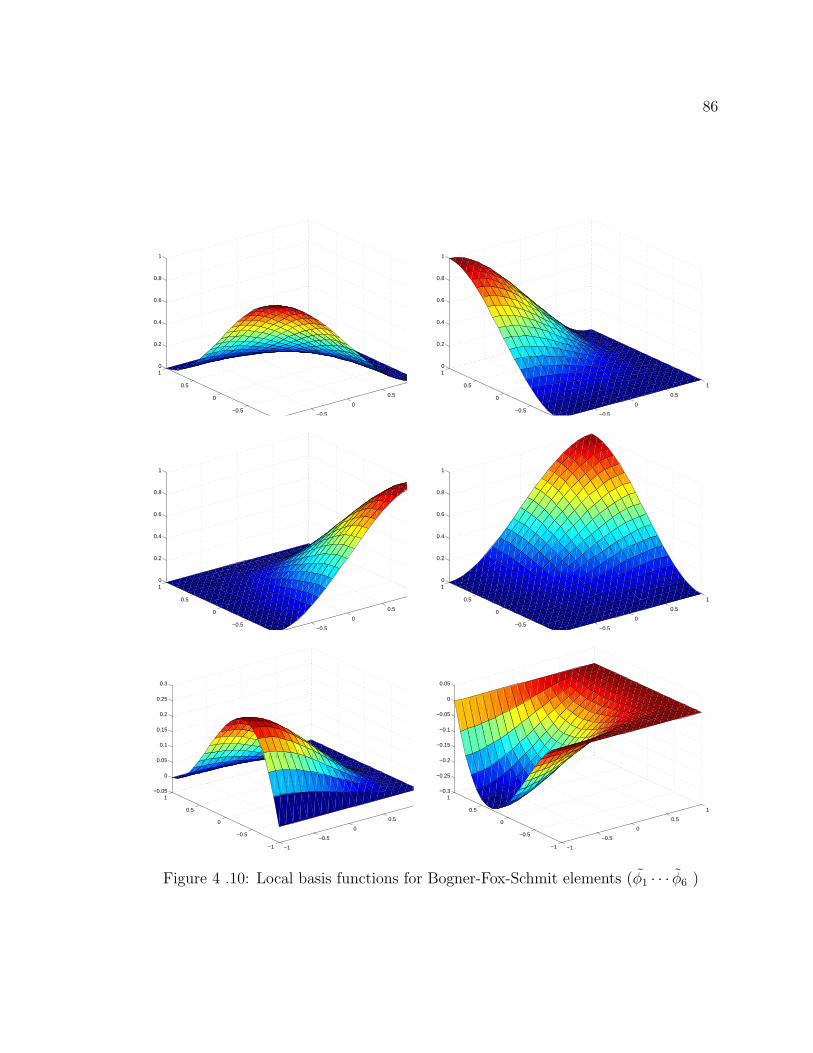
86
−1
−0.5
0
0.5
1
−1
−0.5
0
0.5
10
0.2
0.4
0.6
0.8
1
−1
−0.5
0
0.5
1
−1
−0.5
0
0.5
10
0.2
0.4
0.6
0.8
1
−1
−0.5
0
0.5
1
−1
−0.5
0
0.5
10
0.2
0.4
0.6
0.8
1
−1
−0.5
0
0.5
1
−1
−0.5
0
0.5
10
0.2
0.4
0.6
0.8
1
−1
−0.5
0
0.5
1
−1
−0.5
0
0.5
1−0.05
0
0.05
0.1
0.15
0.2
0.25
0.3
−1
−0.5
0
0.5
1
−1
−0.5
0
0.5
1−0.3
−0.25
−0.2
−0.15
−0.1
−0.05
0
0.05
Figure 4 .10: Local basis functions for Bogner-Fox-Schmit elements (φ1 · · · φ6 )
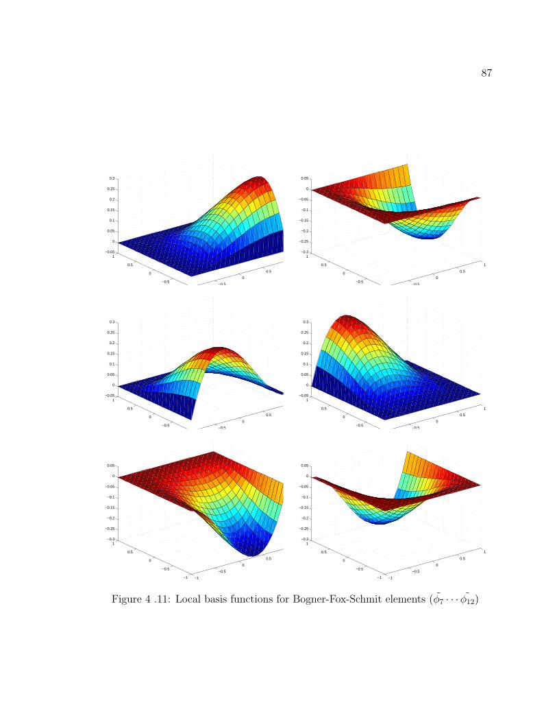
87
−1
−0.5
0
0.5
1
−1
−0.5
0
0.5
1−0.05
0
0.05
0.1
0.15
0.2
0.25
0.3
−1
−0.5
0
0.5
1
−1
−0.5
0
0.5
1−0.3
−0.25
−0.2
−0.15
−0.1
−0.05
0
0.05
−1
−0.5
0
0.5
1
−1
−0.5
0
0.5
1−0.05
0
0.05
0.1
0.15
0.2
0.25
0.3
−1
−0.5
0
0.5
1
−1
−0.5
0
0.5
1−0.05
0
0.05
0.1
0.15
0.2
0.25
0.3
−1
−0.5
0
0.5
1
−1
−0.5
0
0.5
1−0.3
−0.25
−0.2
−0.15
−0.1
−0.05
0
0.05
−1
−0.5
0
0.5
1
−1
−0.5
0
0.5
1−0.3
−0.25
−0.2
−0.15
−0.1
−0.05
0
0.05
Figure 4 .11: Local basis functions for Bogner-Fox-Schmit elements (φ7 · · · φ12)

88
−1
−0.5
0
0.5
1
−1
−0.5
0
0.5
10
0.02
0.04
0.06
0.08
0.1
−1
−0.5
0
0.5
1
−1
−0.5
0
0.5
1−0.1
−0.08
−0.06
−0.04
−0.02
0
0.02
−1
−0.5
0
0.5
1
−1
−0.5
0
0.5
1−0.1
−0.08
−0.06
−0.04
−0.02
0
0.02
−1
−0.5
0
0.5
1
−1
−0.5
0
0.5
10
0.02
0.04
0.06
0.08
0.1
Figure 4 .12: Local basis functions for Bogner-Fox-Schmit elements (φ13 · · · φ16)

89
4.7 Discretizing the Continuous Problem
Let φi : i = 1, . . . , m denote the global basis functions, defined on ΩH . We want to
approximate ψ(x, y) by a function ψH in the space SH = span φi : i = 1, . . . , m.As ψH(x, y) lies in SH we may expand:
ψH(x, y) =m∑
j=1
cjφj(x, y). (4 .18)
Now, the problem is computing the coefficients cj’s in ( 4 .18). Taking the variation
of ( 4 .2) over SH gives the variational equations which ψH(x, y) satisfies :
a(ψH , φH) + b(ψH , ψH , φH) = (f, curl φH), for all φH ∈ SH . (4 .19)
Setting φH = φi(x, y) in ( 4 .19) and substituting ( 4 .18) into ( 4 .19) yields
m∑j=1
cja(φj, φi) +m∑
j=1
m∑
k=1
cjckb(φj, φk, φi) = (f, curl φi), i = 1, ..,m. (4 .20)
Alternately, we may represent ( 4 .20) as a m×m nonlinear system :
G(C) = AC +
CT B(1)C
CT B(2)C
.
.
CT B(m)C
= L, (4 .21)
90
where
Aij = a(φj, φi),
B(i)jk = b(φj, φk, φi),
Li = (f, curl φi),
C =
c1
c2
.
.
.
cm−1
cm.
In another form, we may rewrite equation ( 4 .21) as :
F (C) = 0,
where F (C) = G(C)− L. (4 .22)
4.8 The Solution of F (C) = 0
In this section, we discuss how to solve the resulting nonlinear system of equations.
We use the Newton’s method for nonlinear systems.
91
Consider the Newton’s iteration
cn+1 = cn − J(cn)−1F (cn),
where F : Rm → Rm is defined in (b4 .22) and J(c) is defined by
J(c) =
∂f1(c)∂x1
. . . ∂f1(c)∂xn
......
∂fn(c)∂x1
. . . ∂fn(c)∂xn
.
It is known that the (n+1)-th error is proportional to the square of the n-th error.
So that the convergence is very rapid once the errors are small. So we need to pick
a good initial guess to solve the nonlinear system of equations. Choosing c0 to be
the zero vector means that the first iteration will give us a solution to a discretized
biharmonic equation. Hence, c1 is a good choice for the initial guess.
One requirement which may be imposed upon any iterative method is that it be
norm-reducing in sense that
‖ F (cn+1) ‖≤‖ F (cn+1) ‖, k = 0, 1, · · · ,
holds in some norm. The Newton method does not necessarily satisfy this require-
ment. One simple modification of Newton method is adding the following IF state-

92
ment
If (‖ F (cn+1) ‖≥‖ F (cn) ‖) then
cn+1 = cn − 1
2J(cn)−1F (cn)
else
cn+1 = cn − J(cn)−1F (cn)
end if
Using the Newton method involves the computing of the Jacobian matrix which will
be described in the next section.
4.9 Computation of the Jacobian
The elements of the Jacobian matrix are given by
Jij =∂Fi
∂Ci
= Aij +m∑
k=1
Ck(b(i)kj + b
(i)jk ),
= a(φj, φi) +m∑
k=1
Ckb(φk, φj, φi) + b(φj, φk, φi).(4 .23)
We assemble Aij , b(i)kj and b
(i)jk element by element as
Aij =nelem∑
l=1
A(l)ij ,
b(i)kj =
nelem∑
l=1
b(i)kj (l),
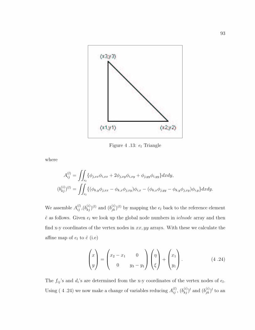
93
Figure 4 .13: el Triangle
where
A(l)ij =
∫∫
el
φj,xxφi,xx + 2φj,xyφi,xy + φj,yyφi,yydxdy,
(b(i)kj )
(l) =
∫∫
el
(φk,yφj,xx − φk,xφj,xy)φi,x − (φk,xφj,yy − φk,yφj,xy)φi,ydxdy.
We assemble A(l)ij ,(b
(i)kj )
(l) and (b(i)jk )(l) by mapping the el back to the reference element
e as follows. Given el we look up the global node numbers in ielnode array and then
find x-y coordinates of the vertex nodes in xx, yy arrays. With these we calculate the
affine map of el to e (i.e)
x
y
=
x2 − x1 0
0 y3 − y1
η
ξ
+
x1
y1
. (4 .24)
The fij’s and di’s are determined from the x-y coordinates of the vertex nodes of el.
Using ( 4 .24) we now make a change of variables reducing A(l)ij , (b
(i)kj )
l and (b(i)jk )l to an

94
integral over e. After applying the chain rule , the final results for the case of morley
elements are :
A(l)ij = h−2
∫∫
e
φi,ξξφj,ξξ + 2φi,ξηφj,ξη + φi,ηηφj,ηη =h−2Aij,
(b(i)jk )(l) = h−2
∫∫
e
(φk,ηφj,ξξ − φk,ξφj,ξη)φi,ξ − (φk,ξφj,ηη − φk,ηφj,ξη)φi,η=h−2b(i)jk ,
(b(i)kj )
(l) = h−2
∫∫
e
(φj,ηφk,ξξ − φj,ξφk,ξη)φi,ξ − (φj,ξφk,ηη − φj,ηφk,ξη)φi,η=h−2b(i)kj ,
where h = x2 − x1 = y3 − y1. In our case we have a regular finite elements. In
Bogner-Fox-Schmit, we have:
A(l)ij =
4
h2Aij,
(b(i)jk )(l) =
4
h2
˜b(i)jk ,
(b(i)kj )
(l) =4
h2
˜b(i)kj ,
where h = 2/lx.Hence, A(l)ij , (b
(i)jk )(l) and (b
(i)kj )
(l) are the same for any element el in the
finite element space. The entries of the matrix A and the three-dimension array b for
the case of Morley triangles can be computed exactly with MATHEMATICA
f[x_,y_]:=f1 x^2+f2 y^2+f3 x y+f4 x+f5 y+f6
fx[x_,y_] = D[ f[x,y] , x ] ;
fy[x_,y_] = D[ f[x,y] , y ] ;
pp1:=Solve[ f[0,0] == 1 ,
f[1,0] == 0 ,
f[0,1] == 0 ,
-fy[1/2,0] == 0 ,
-fx[0,1/2] == 0 ,

95
fx[1/2,1/2] + fy[1/2,1/2] == 0 Sqrt[2] ,
f1,f2,f3,f4,f5,f6 ]
v1:=f1,f2,f3,f4,f5,f6 /. pp1
r1:=1.v1
pp2:=Solve[ f[0,0] == 0 ,
f[1,0] == 1 ,
f[0,1] == 0 ,
-fy[1/2,0] == 0 ,
-fx[0,1/2] == 0 ,
fx[1/2,1/2] + fy[1/2,1/2] == 0 Sqrt[2] ,
f1,f2,f3,f4,f5,f6 ]
v2:=f1,f2,f3,f4,f5,f6 /. pp2
r2:=1.v2
pp3:=Solve[ f[0,0] == 0 ,
f[1,0] == 0 ,
f[0,1] == 1 ,
-fy[1/2,0] == 0 ,
-fx[0,1/2] == 0 ,
fx[1/2,1/2] + fy[1/2,1/2] == 0 Sqrt[2] ,
f1,f2,f3,f4,f5,f6 ]
v3:=f1,f2,f3,f4,f5,f6 /. pp3
r3:=1.v3
pp4:=Solve[ f[0,0] == 0 ,
f[1,0] == 0 ,
f[0,1] == 0 ,
-fy[1/2,0] == 1 ,

96
-fx[0,1/2] == 0 ,
fx[1/2,1/2] + fy[1/2,1/2] == 0 Sqrt[2] ,
f1,f2,f3,f4,f5,f6 ]
v4:=f1,f2,f3,f4,f5,f6 /. pp4
r4:=1.v4
pp5:=Solve[ f[0,0] == 0 ,
f[1,0] == 0 ,
f[0,1] == 0 ,
-fy[1/2,0] == 0 ,
-fx[0,1/2] == 0 ,
fx[1/2,1/2] + fy[1/2,1/2] == 1 Sqrt[2] ,
f1,f2,f3,f4,f5,f6 ]
v5:=f1,f2,f3,f4,f5,f6 /. pp5
r5:=1.v5
pp6:=Solve[ f[0,0] == 0 ,
f[1,0] == 0 ,
f[0,1] == 0 ,
-fy[1/2,0] == 0 ,
-fx[0,1/2] == 1 ,
fx[1/2,1/2] + fy[1/2,1/2] == 0 Sqrt[2] ,
f1,f2,f3,f4,f5,f6 ]
v6:=f1,f2,f3,f4,f5,f6 /. pp6
r6:=1.v6
a = r1,r2,r3,r4,r5,r6
e1=f[x,y] /. pp1 ;
phi[1,x_,y_] = 1.e1
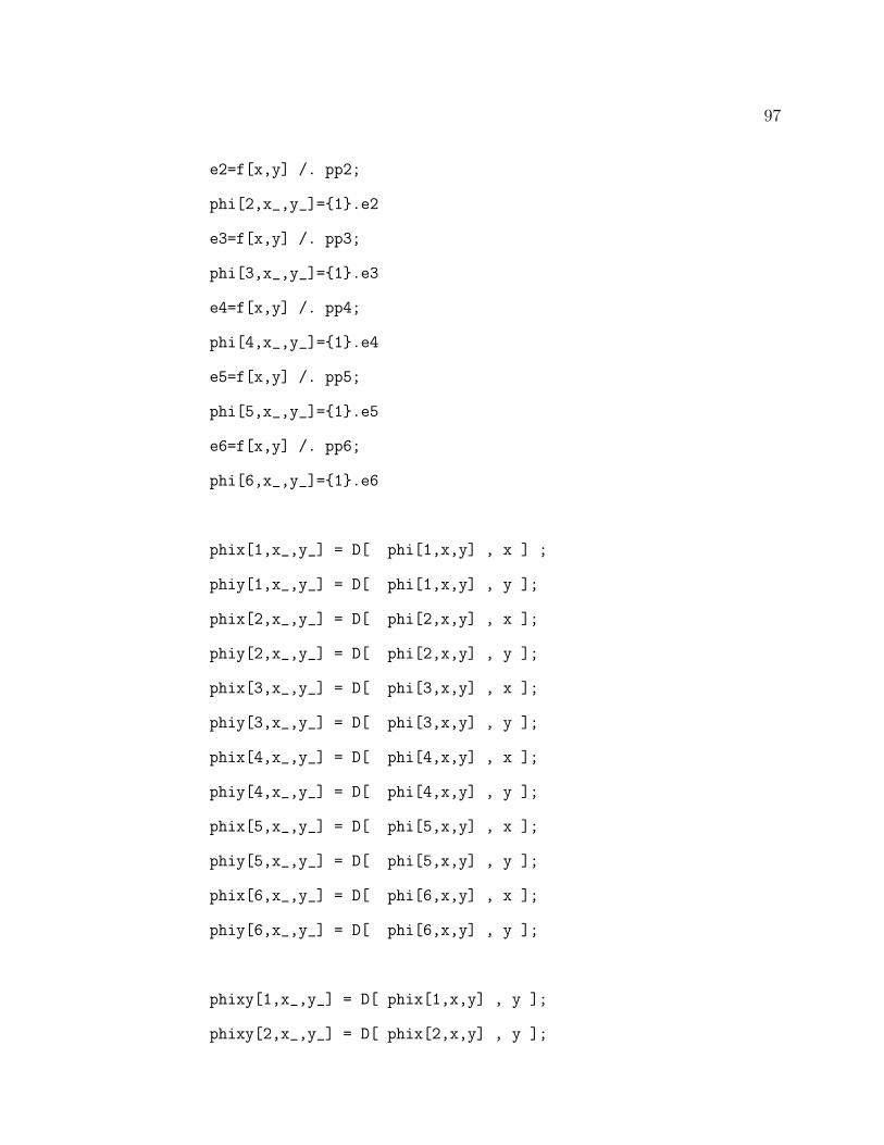
97
e2=f[x,y] /. pp2;
phi[2,x_,y_]=1.e2
e3=f[x,y] /. pp3;
phi[3,x_,y_]=1.e3
e4=f[x,y] /. pp4;
phi[4,x_,y_]=1.e4
e5=f[x,y] /. pp5;
phi[5,x_,y_]=1.e5
e6=f[x,y] /. pp6;
phi[6,x_,y_]=1.e6
phix[1,x_,y_] = D[ phi[1,x,y] , x ] ;
phiy[1,x_,y_] = D[ phi[1,x,y] , y ];
phix[2,x_,y_] = D[ phi[2,x,y] , x ];
phiy[2,x_,y_] = D[ phi[2,x,y] , y ];
phix[3,x_,y_] = D[ phi[3,x,y] , x ];
phiy[3,x_,y_] = D[ phi[3,x,y] , y ];
phix[4,x_,y_] = D[ phi[4,x,y] , x ];
phiy[4,x_,y_] = D[ phi[4,x,y] , y ];
phix[5,x_,y_] = D[ phi[5,x,y] , x ];
phiy[5,x_,y_] = D[ phi[5,x,y] , y ];
phix[6,x_,y_] = D[ phi[6,x,y] , x ];
phiy[6,x_,y_] = D[ phi[6,x,y] , y ];
phixy[1,x_,y_] = D[ phix[1,x,y] , y ];
phixy[2,x_,y_] = D[ phix[2,x,y] , y ];
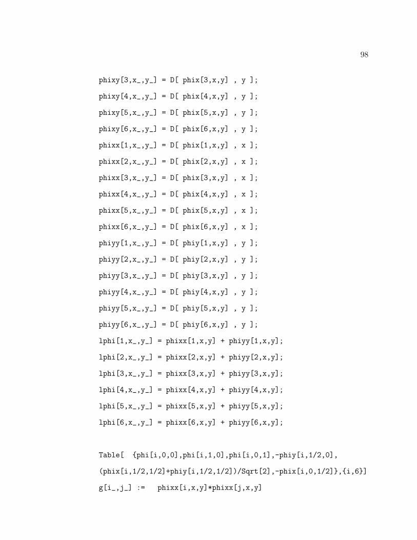
98
phixy[3,x_,y_] = D[ phix[3,x,y] , y ];
phixy[4,x_,y_] = D[ phix[4,x,y] , y ];
phixy[5,x_,y_] = D[ phix[5,x,y] , y ];
phixy[6,x_,y_] = D[ phix[6,x,y] , y ];
phixx[1,x_,y_] = D[ phix[1,x,y] , x ];
phixx[2,x_,y_] = D[ phix[2,x,y] , x ];
phixx[3,x_,y_] = D[ phix[3,x,y] , x ];
phixx[4,x_,y_] = D[ phix[4,x,y] , x ];
phixx[5,x_,y_] = D[ phix[5,x,y] , x ];
phixx[6,x_,y_] = D[ phix[6,x,y] , x ];
phiyy[1,x_,y_] = D[ phiy[1,x,y] , y ];
phiyy[2,x_,y_] = D[ phiy[2,x,y] , y ];
phiyy[3,x_,y_] = D[ phiy[3,x,y] , y ];
phiyy[4,x_,y_] = D[ phiy[4,x,y] , y ];
phiyy[5,x_,y_] = D[ phiy[5,x,y] , y ];
phiyy[6,x_,y_] = D[ phiy[6,x,y] , y ];
lphi[1,x_,y_] = phixx[1,x,y] + phiyy[1,x,y];
lphi[2,x_,y_] = phixx[2,x,y] + phiyy[2,x,y];
lphi[3,x_,y_] = phixx[3,x,y] + phiyy[3,x,y];
lphi[4,x_,y_] = phixx[4,x,y] + phiyy[4,x,y];
lphi[5,x_,y_] = phixx[5,x,y] + phiyy[5,x,y];
lphi[6,x_,y_] = phixx[6,x,y] + phiyy[6,x,y];
Table[ phi[i,0,0],phi[i,1,0],phi[i,0,1],-phiy[i,1/2,0],
(phix[i,1/2,1/2]+phiy[i,1/2,1/2])/Sqrt[2],-phix[i,0,1/2],i,6]
g[i_,j_] := phixx[i,x,y]*phixx[j,x,y]
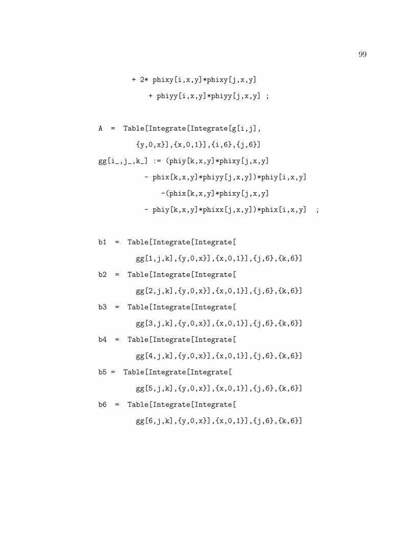
99
+ 2* phixy[i,x,y]*phixy[j,x,y]
+ phiyy[i,x,y]*phiyy[j,x,y] ;
A = Table[Integrate[Integrate[g[i,j],
y,0,x],x,0,1],i,6,j,6]
gg[i_,j_,k_] := (phiy[k,x,y]*phixy[j,x,y]
- phix[k,x,y]*phiyy[j,x,y])*phiy[i,x,y]
-(phix[k,x,y]*phixy[j,x,y]
- phiy[k,x,y]*phixx[j,x,y])*phix[i,x,y] ;
b1 = Table[Integrate[Integrate[
gg[1,j,k],y,0,x],x,0,1],j,6,k,6]
b2 = Table[Integrate[Integrate[
gg[2,j,k],y,0,x],x,0,1],j,6,k,6]
b3 = Table[Integrate[Integrate[
gg[3,j,k],y,0,x],x,0,1],j,6,k,6]
b4 = Table[Integrate[Integrate[
gg[4,j,k],y,0,x],x,0,1],j,6,k,6]
b5 = Table[Integrate[Integrate[
gg[5,j,k],y,0,x],x,0,1],j,6,k,6]
b6 = Table[Integrate[Integrate[
gg[6,j,k],y,0,x],x,0,1],j,6,k,6]
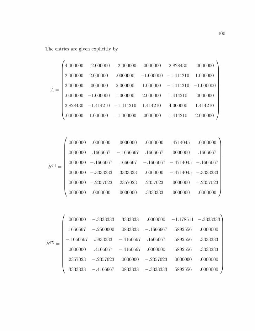
100
The entries are given explicitly by
A =
4.000000 −2.000000 −2.000000 .0000000 2.828430 .0000000
2.000000 2.000000 .0000000 −1.000000 −1.414210 1.000000
2.000000 .0000000 2.000000 1.000000 −1.414210 −1.000000
.0000000 −1.000000 1.000000 2.000000 1.414210 .0000000
2.828430 −1.414210 −1.414210 1.414210 4.000000 1.414210
.0000000 1.000000 −1.000000 .0000000 1.414210 2.000000
B(1) =
.0000000 .0000000 .0000000 .0000000 .4714045 .0000000
.0000000 .1666667 −.1666667 .1666667 .0000000 .1666667
.0000000 −.1666667 .1666667 −.1666667 −.4714045 −.1666667
.0000000 −.3333333 .3333333 .0000000 −.4714045 −.3333333
.0000000 −.2357023 .2357023 .2357023 .0000000 −.2357023
.0000000 .0000000 .0000000 .3333333 .0000000 .0000000
B(2) =
.0000000 −.3333333 .3333333 .0000000 −1.178511 −.3333333
.1666667 −.2500000 .0833333 −.1666667 .5892556 .0000000
−.1666667 .5833333 −.4166667 .1666667 .5892556 .3333333
.0000000 .4166667 −.4166667 .0000000 .5892556 .3333333
.2357023 −.2357023 .0000000 −.2357023 .0000000 .0000000
.3333333 −.4166667 .0833333 −.3333333 .5892556 .0000000

101
B(3) =
.0000000 .3333333 −.3333333 .0000000 .7071068 .3333333
−.1666667 .0833333 .0833333 .0000000 −.5892556 −.1666667
.1666667 −.4166667 .2500000 .0000000 −.1178511 −.1666667
.0000000 −.0833333 .0833333 .0000000 −.1178511 .0000000
−.2357023 .4714045 −.2357023 .0000000 .0000000 .2357023
−.3333333 .4166667 −.0833333 .0000000 −.5892556 .0000000
B(4) =
.0000000 .0000000 .0000000 .3333333 .0000000 .0000000
.1666667 −.1666667 .0000000 −.1666667 .0000000 .0000000
−.1666667 .1666667 .0000000 −.1666667 .0000000 .0000000
−.3333333 .3333333 .0000000 .0000000 .0000000 .0000000
−.2357023 .2357023 .0000000 .2357023 .0000000 .0000000
.0000000 .0000000 .0000000 .0000000 .0000000 .0000000
B(5) =
.4714045 −1.1785113 .7071068 .0000000 .0000000 −.4714045
.0000000 .5892556 −.5892556 .0000000 .8333333 .4714045
−.4714045 .5892556 −.1178511 .0000000 −.8333333 .0000000
.0000000 −.5892556 .5892556 .0000000 −.8333333 −.4714045
.6666667 −1.6666667 1.0000000 .0000000 .0000000 −.6666667
.4714045 −.5892556 .1178511 .0000000 .8333333 .0000000
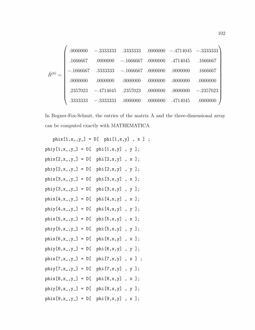
102
B(6) =
.0000000 −.3333333 .3333333 .0000000 −.4714045 −.3333333
.1666667 .0000000 −.1666667 .0000000 .4714045 .1666667
−.1666667 .3333333 −.1666667 .0000000 .0000000 .1666667
.0000000 .0000000 .0000000 .0000000 .0000000 .0000000
.2357023 −.4714045 .2357023 .0000000 .0000000 −.2357023
.3333333 −.3333333 .0000000 .0000000 .4714045 .0000000
In Bogner-Fox-Schmit, the entries of the matrix A and the three-dimensional array
can be computed exactly with MATHEMATICA
phix[1,x_,y_] = D[ phi[1,x,y] , x ] ;
phiy[1,x_,y_] = D[ phi[1,x,y] , y ];
phix[2,x_,y_] = D[ phi[2,x,y] , x ];
phiy[2,x_,y_] = D[ phi[2,x,y] , y ];
phix[3,x_,y_] = D[ phi[3,x,y] , x ];
phiy[3,x_,y_] = D[ phi[3,x,y] , y ];
phix[4,x_,y_] = D[ phi[4,x,y] , x ];
phiy[4,x_,y_] = D[ phi[4,x,y] , y ];
phix[5,x_,y_] = D[ phi[5,x,y] , x ];
phiy[5,x_,y_] = D[ phi[5,x,y] , y ];
phix[6,x_,y_] = D[ phi[6,x,y] , x ];
phiy[6,x_,y_] = D[ phi[6,x,y] , y ];
phix[7,x_,y_] = D[ phi[7,x,y] , x ] ;
phiy[7,x_,y_] = D[ phi[7,x,y] , y ];
phix[8,x_,y_] = D[ phi[8,x,y] , x ];
phiy[8,x_,y_] = D[ phi[8,x,y] , y ];
phix[9,x_,y_] = D[ phi[9,x,y] , x ];

103
phiy[9,x_,y_] = D[ phi[9,x,y] , y ];
phix[10,x_,y_] = D[ phi[10,x,y] , x ];
phiy[10,x_,y_] = D[ phi[10,x,y] , y ];
phix[11,x_,y_] = D[ phi[11,x,y] , x ] ;
phiy[11,x_,y_] = D[ phi[11,x,y] , y ];
phix[12,x_,y_] = D[ phi[12,x,y] , x ];
phiy[12,x_,y_] = D[ phi[12,x,y] , y ];
phix[13,x_,y_] = D[ phi[13,x,y] , x ];
phiy[13,x_,y_] = D[ phi[13,x,y] , y ];
phix[14,x_,y_] = D[ phi[14,x,y] , x ];
phiy[14,x_,y_] = D[ phi[14,x,y] , y ];
phix[15,x_,y_] = D[ phi[15,x,y] , x ];
phiy[15,x_,y_] = D[ phi[15,x,y] , y ];
phix[16,x_,y_] = D[ phi[16,x,y] , x ];
phiy[16,x_,y_] = D[ phi[16,x,y] , y ];
phixy[1,x_,y_] = D[ phix[1,x,y] , y ];
phixy[2,x_,y_] = D[ phix[2,x,y] , y ];
phixy[3,x_,y_] = D[ phix[3,x,y] , y ];
phixy[4,x_,y_] = D[ phix[4,x,y] , y ];
phixy[5,x_,y_] = D[ phix[5,x,y] , y ];
phixy[6,x_,y_] = D[ phix[6,x,y] , y ];
phixy[7,x_,y_] = D[ phix[7,x,y] , y ];
phixy[8,x_,y_] = D[ phix[8,x,y] , y ];
phixy[9,x_,y_] = D[ phix[9,x,y] , y ];
phixy[10,x_,y_] = D[ phix[10,x,y] , y ];

104
phixy[11,x_,y_] = D[ phix[11,x,y] , y ];
phixy[12,x_,y_] = D[ phix[12,x,y] , y ];
phixy[13,x_,y_] = D[ phix[13,x,y] , y ];
phixy[14,x_,y_] = D[ phix[14,x,y] , y ];
phixy[15,x_,y_] = D[ phix[15,x,y] , y ];
phixy[16,x_,y_] = D[ phix[16,x,y] , y ];
phixx[1,x_,y_] = D[ phix[1,x,y] , x ];
phixx[2,x_,y_] = D[ phix[2,x,y] , x ];
phixx[3,x_,y_] = D[ phix[3,x,y] , x ];
phixx[4,x_,y_] = D[ phix[4,x,y] , x ];
phixx[5,x_,y_] = D[ phix[5,x,y] , x ];
phixx[6,x_,y_] = D[ phix[6,x,y] , x ];
phixx[7,x_,y_] = D[ phix[7,x,y] , x ];
phixx[8,x_,y_] = D[ phix[8,x,y] , x ];
phixx[9,x_,y_] = D[ phix[9,x,y] , x ];
phixx[10,x_,y_] = D[ phix[10,x,y] , x ];
phixx[11,x_,y_] = D[ phix[11,x,y] , x ];
phixx[12,x_,y_] = D[ phix[12,x,y] , x ];
phixx[13,x_,y_] = D[ phix[13,x,y] , x ];
phixx[14,x_,y_] = D[ phix[14,x,y] , x ];
phixx[15,x_,y_] = D[ phix[15,x,y] , x ];
phixx[16,x_,y_] = D[ phix[16,x,y] , x ];
phiyy[1,x_,y_] = D[ phiy[1,x,y] , y ];
phiyy[2,x_,y_] = D[ phiy[2,x,y] , y ];
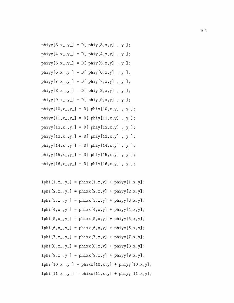
105
phiyy[3,x_,y_] = D[ phiy[3,x,y] , y ];
phiyy[4,x_,y_] = D[ phiy[4,x,y] , y ];
phiyy[5,x_,y_] = D[ phiy[5,x,y] , y ];
phiyy[6,x_,y_] = D[ phiy[6,x,y] , y ];
phiyy[7,x_,y_] = D[ phiy[7,x,y] , y ];
phiyy[8,x_,y_] = D[ phiy[8,x,y] , y ];
phiyy[9,x_,y_] = D[ phiy[9,x,y] , y ];
phiyy[10,x_,y_] = D[ phiy[10,x,y] , y ];
phiyy[11,x_,y_] = D[ phiy[11,x,y] , y ];
phiyy[12,x_,y_] = D[ phiy[12,x,y] , y ];
phiyy[13,x_,y_] = D[ phiy[13,x,y] , y ];
phiyy[14,x_,y_] = D[ phiy[14,x,y] , y ];
phiyy[15,x_,y_] = D[ phiy[15,x,y] , y ];
phiyy[16,x_,y_] = D[ phiy[16,x,y] , y ];
lphi[1,x_,y_] = phixx[1,x,y] + phiyy[1,x,y];
lphi[2,x_,y_] = phixx[2,x,y] + phiyy[2,x,y];
lphi[3,x_,y_] = phixx[3,x,y] + phiyy[3,x,y];
lphi[4,x_,y_] = phixx[4,x,y] + phiyy[4,x,y];
lphi[5,x_,y_] = phixx[5,x,y] + phiyy[5,x,y];
lphi[6,x_,y_] = phixx[6,x,y] + phiyy[6,x,y];
lphi[7,x_,y_] = phixx[7,x,y] + phiyy[7,x,y];
lphi[8,x_,y_] = phixx[8,x,y] + phiyy[8,x,y];
lphi[9,x_,y_] = phixx[9,x,y] + phiyy[9,x,y];
lphi[10,x_,y_] = phixx[10,x,y] + phiyy[10,x,y];
lphi[11,x_,y_] = phixx[11,x,y] + phiyy[11,x,y];
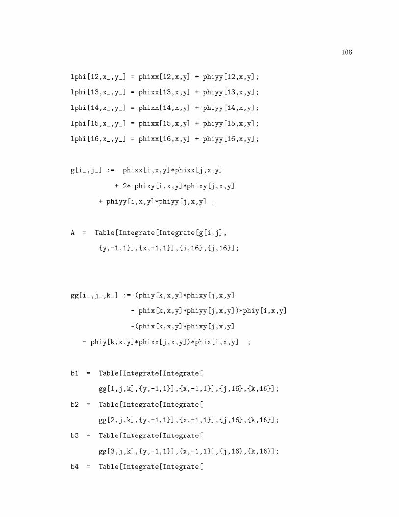
106
lphi[12,x_,y_] = phixx[12,x,y] + phiyy[12,x,y];
lphi[13,x_,y_] = phixx[13,x,y] + phiyy[13,x,y];
lphi[14,x_,y_] = phixx[14,x,y] + phiyy[14,x,y];
lphi[15,x_,y_] = phixx[15,x,y] + phiyy[15,x,y];
lphi[16,x_,y_] = phixx[16,x,y] + phiyy[16,x,y];
g[i_,j_] := phixx[i,x,y]*phixx[j,x,y]
+ 2* phixy[i,x,y]*phixy[j,x,y]
+ phiyy[i,x,y]*phiyy[j,x,y] ;
A = Table[Integrate[Integrate[g[i,j],
y,-1,1],x,-1,1],i,16,j,16];
gg[i_,j_,k_] := (phiy[k,x,y]*phixy[j,x,y]
- phix[k,x,y]*phiyy[j,x,y])*phiy[i,x,y]
-(phix[k,x,y]*phixy[j,x,y]
- phiy[k,x,y]*phixx[j,x,y])*phix[i,x,y] ;
b1 = Table[Integrate[Integrate[
gg[1,j,k],y,-1,1],x,-1,1],j,16,k,16];
b2 = Table[Integrate[Integrate[
gg[2,j,k],y,-1,1],x,-1,1],j,16,k,16];
b3 = Table[Integrate[Integrate[
gg[3,j,k],y,-1,1],x,-1,1],j,16,k,16];
b4 = Table[Integrate[Integrate[

107
gg[4,j,k],y,-1,1],x,-1,1],j,16,k,16];
b5 = Table[Integrate[Integrate[
gg[5,j,k],y,-1,1],x,-1,1],j,16,k,16];
b6 = Table[Integrate[Integrate[
gg[6,j,k],y,-1,1],x,-1,1],j,16,k,16];
b7 = Table[Integrate[Integrate[
gg[7,j,k],y,-1,1],x,-1,1],j,16,k,16];
b8 = Table[Integrate[Integrate[
gg[8,j,k],y,-1,1],x,-1,1],j,16,k,16];
b9 = Table[Integrate[Integrate[
gg[9,j,k],y,-1,1],x,-1,1],j,16,k,16];
b10 = Table[Integrate[Integrate[
gg[10,j,k],y,-1,1],x,-1,1],j,16,k,16];
b11 = Table[Integrate[Integrate[
gg[11,j,k],y,-1,1],x,-1,1],j,16,k,16];
b12 = Table[Integrate[Integrate[
gg[12,j,k],y,-1,1],x,-1,1],j,16,k,16];
b13 = Table[Integrate[Integrate[
gg[13,j,k],y,-1,1],x,-1,1],j,16,k,16];
b14 = Table[Integrate[Integrate[
gg[14,j,k],y,-1,1],x,-1,1],j,16,k,16];
b15 = Table[Integrate[Integrate[
gg[15,j,k],y,-1,1],x,-1,1],j,16,k,16];
b16 = Table[Integrate[Integrate[
gg[16,j,k],y,-1,1],x,-1,1],j,16,k,16];
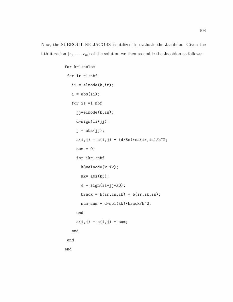
108
Now, the SUBROUTINE JACOBS is utilized to evaluate the Jacobian. Given the
i-th iteration (c1, . . . , cm) of the solution we then assemble the Jacobian as follows:
for k=1:nelem
for ir =1:nbf
ii = elnode(k,ir);
i = abs(ii);
for is =1:nbf
jj=elnode(k,is);
d=sign(ii*jj);
j = abs(jj);
a(i,j) = a(i,j) + (d/Re)*ea(ir,is)/h^2;
sum = 0;
for ik=1:nbf
k3=elnode(k,ik);
kk= abs(k3);
d = sign(ii*jj*k3);
brack = b(ir,is,ik) + b(ir,ik,is);
sum=sum + d*sol(kk)*brack/h^2;
end
a(i,j) = a(i,j) + sum;
end
end
end
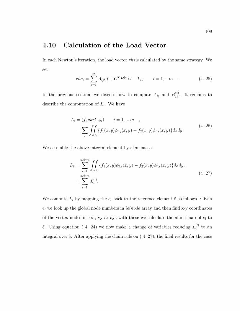
109
4.10 Calculation of the Load Vector
In each Newton’s iteration, the load vector rhsis calculated by the same strategy. We
set
rhsi =m∑
j=1
Aijcj + CT B(i)C − Li, i = 1, ...m . (4 .25)
In the previous section, we discuss how to compute Aij and B(i)jk . It remains to
describe the computation of Li. We have
Li = (f, curl φi) i = 1, .., m ,
=∑
l
∫∫
el
f1(x, y)φi,y(x, y)− f2(x, y)φi,x(x, y)dxdy.(4 .26)
We assemble the above integral element by element as
Li =nelem∑
l=1
∫∫
el
f1(x, y)φi,y(x, y)− f2(x, y)φi,x(x, y)dxdy,
=nelem∑
l=1
L(l)i .
(4 .27)
We compute Li by mapping the el back to the reference element e as follows. Given
el we look up the global node numbers in ielnode array and then find x-y coordinates
of the vertex nodes in xx , yy arrays with these we calculate the affine map of el to
e. Using equation ( 4 .24) we now make a change of variables reducing L(l)i to an
integral over e. After applying the chain rule on ( 4 .27), the final results for the case
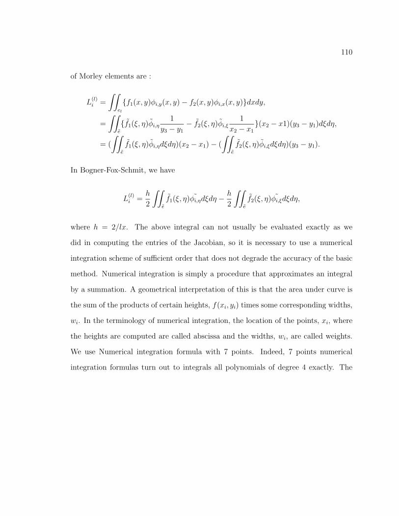
110
of Morley elements are :
L(l)i =
∫∫
el
f1(x, y)φi,y(x, y)− f2(x, y)φi,x(x, y)dxdy,
=
∫∫
e
f1(ξ, η)φi,η1
y3 − y1
− f2(ξ, η)φi,ξ1
x2 − x1
(x2 − x1)(y3 − y1)dξdη,
= (
∫∫
e
f1(ξ, η)φi,ηdξdη)(x2 − x1)− (
∫∫
e
f2(ξ, η)φi,ξdξdη)(y3 − y1).
In Bogner-Fox-Schmit, we have
L(l)i =
h
2
∫∫
e
f1(ξ, η)φi,ηdξdη − h
2
∫∫
e
f2(ξ, η)φi,ξdξdη,
where h = 2/lx. The above integral can not usually be evaluated exactly as we
did in computing the entries of the Jacobian, so it is necessary to use a numerical
integration scheme of sufficient order that does not degrade the accuracy of the basic
method. Numerical integration is simply a procedure that approximates an integral
by a summation. A geometrical interpretation of this is that the area under curve is
the sum of the products of certain heights, f(xi, yi) times some corresponding widths,
wi. In the terminology of numerical integration, the location of the points, xi, where
the heights are computed are called abscissa and the widths, wi, are called weights.
We use Numerical integration formula with 7 points. Indeed, 7 points numerical
integration formulas turn out to integrals all polynomials of degree 4 exactly. The

111
numerical integration points (abscissa) (ξ, η) and the weights ωi are given below
ξ =
0
1/2
1
1/2
0
0
1/3
η =
0
0
0
1/2
1
1/2
1/3
ω =
1/40
1/15
1/40
1/15
1/40
1/15
9/40
.
In the case of rectangles, we use numerical integration formula with 4 points. Indeed,
4 points numerical integration formulas turn out to integrals all bicubic polynomials
exactly. The numerical integration points (abscissa)(ξ, η) and the weights wi are
below
ξ =
−1√3
1√3
− 1√3
1√3
η =
− 1√3
−1√3
1√3
1√3
w =
1
1
1
1
.
4.11 Storage of the Jacobian
The efficiency of any iterative linear solver is determined primarily by the perfor-
mance of the matrix-vector product and therefore on the storage scheme used for the
matrix. The coefficient matrix of the Jacobian is sparse. Large-scale linear systems
of the form Ax = b can be most efficiently solved if the zero elements of J are not
stored. There are many methods for solving the non-zero elements of a sparse matrix.
The Compressed Row and Column Storage Formats are most general. They make ab-
solutely no assumptions about the sparsity structure of the matrix. The compressed
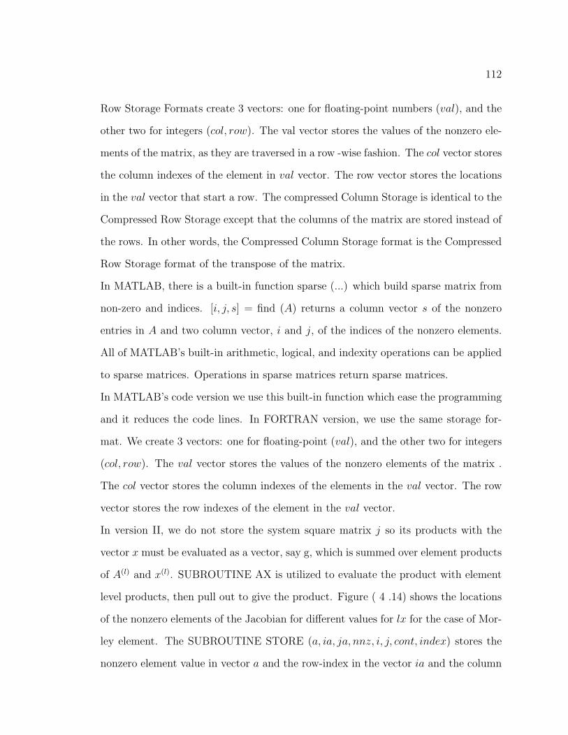
112
Row Storage Formats create 3 vectors: one for floating-point numbers (val), and the
other two for integers (col, row). The val vector stores the values of the nonzero ele-
ments of the matrix, as they are traversed in a row -wise fashion. The col vector stores
the column indexes of the element in val vector. The row vector stores the locations
in the val vector that start a row. The compressed Column Storage is identical to the
Compressed Row Storage except that the columns of the matrix are stored instead of
the rows. In other words, the Compressed Column Storage format is the Compressed
Row Storage format of the transpose of the matrix.
In MATLAB, there is a built-in function sparse (...) which build sparse matrix from
non-zero and indices. [i, j, s] = find (A) returns a column vector s of the nonzero
entries in A and two column vector, i and j, of the indices of the nonzero elements.
All of MATLAB’s built-in arithmetic, logical, and indexity operations can be applied
to sparse matrices. Operations in sparse matrices return sparse matrices.
In MATLAB’s code version we use this built-in function which ease the programming
and it reduces the code lines. In FORTRAN version, we use the same storage for-
mat. We create 3 vectors: one for floating-point (val), and the other two for integers
(col, row). The val vector stores the values of the nonzero elements of the matrix .
The col vector stores the column indexes of the elements in the val vector. The row
vector stores the row indexes of the element in the val vector.
In version II, we do not store the system square matrix j so its products with the
vector x must be evaluated as a vector, say g, which is summed over element products
of A(l) and x(l). SUBROUTINE AX is utilized to evaluate the product with element
level products, then pull out to give the product. Figure ( 4 .14) shows the locations
of the nonzero elements of the Jacobian for different values for lx for the case of Mor-
ley element. The SUBROUTINE STORE (a, ia, ja, nnz, i, j, cont, index) stores the
nonzero element value in vector a and the row-index in the vector ia and the column
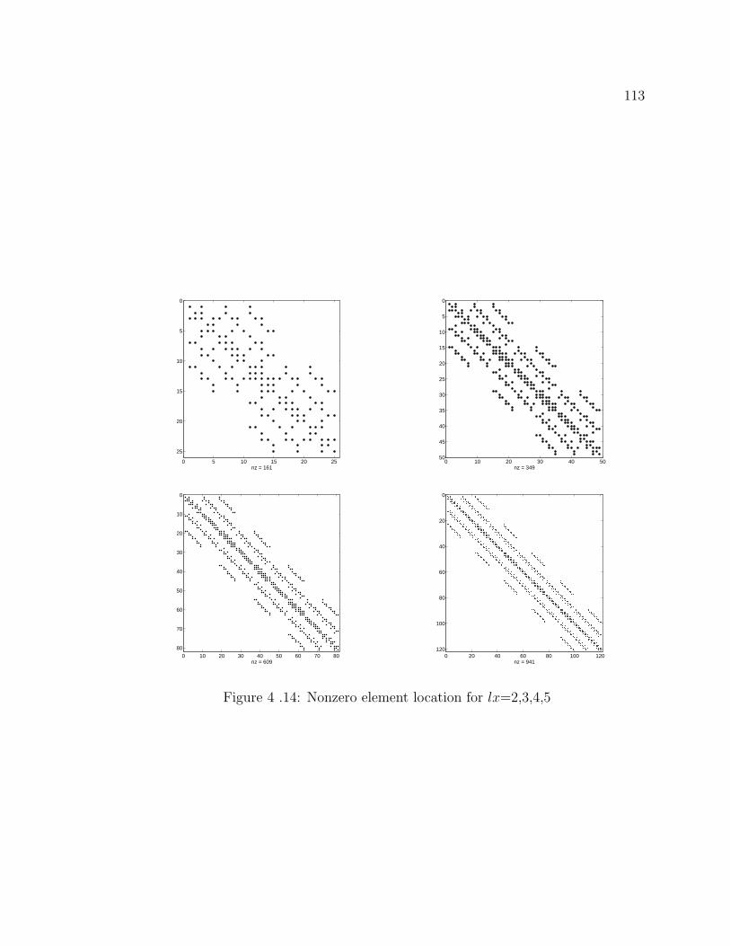
113
0 5 10 15 20 25
0
5
10
15
20
25
nz = 1610 10 20 30 40 50
0
5
10
15
20
25
30
35
40
45
50
nz = 349
0 10 20 30 40 50 60 70 80
0
10
20
30
40
50
60
70
80
nz = 6090 20 40 60 80 100 120
0
20
40
60
80
100
120
nz = 941
Figure 4 .14: Nonzero element location for lx=2,3,4,5

114
indices in the vector ja.
4.12 Boundary Conditions Contribution
In SUBROUTINE JACOBS, we assemble the contributions to the Jacobian that
are independent of the boundary conditions. The matrix resulting from the calcu-
lations in SUBROUTINE JACOBS is called the primitive stiffness matrix. Finally,
in SUBROUTINES BOUNDARY-A(...) and BOUNDARY-RHS(...) the boundary
conditions are added on as an extra set of linear equations. The boundary node num-
ber are generated by the SUBROUTINE MAELNODE and stored in the vector ibo.
The calculation works as follows. Now, we list some information about the Jacobian
matrix.
Morley elements
Number of boundary points = 4lx = bp
Number of normal boundary points = 4lx = bn
Number of interior points = (lx− 1)2 = ip
Number of normal interior points = lx(3lx− 2) = in
Number of non-zero elements in the
Jacobian corresponds to boundary points = 12(bp− 4) + 2(6) + 2(9)
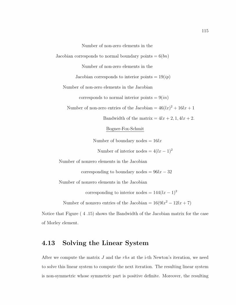
115
Number of non-zero elements in the
Jacobian corresponds to normal boundary points = 6(bn)
Number of non-zero elements in the
Jacobian corresponds to interior points = 19(ip)
Number of non-zero elements in the Jacobian
corresponds to normal interior points = 9(in)
Number of non-zero entries of the Jacobian = 46(lx)2 + 16lx + 1
Bandwidth of the matrix = 4lx + 2, 1, 4lx + 2.
Bogner-Fox-Schmit
Number of boundary nodes = 16lx
Number of interior nodes = 4(lx− 1)2
Number of nonzero elements in the Jacobian
corresponding to boundary nodes = 96lx− 32
Number of nonzero elements in the Jacobian
corresponding to interior nodes = 144(lx− 1)2
Number of nonzero entries of the Jacobian = 16(9lx2 − 12lx + 7)
Notice that Figure ( 4 .15) shows the Bandwidth of the Jacobian matrix for the case
of Morley element.
4.13 Solving the Linear System
After we compute the matrix J and the rhs at the i-th Newton’s iteration, we need
to solve this linear system to compute the next iteration. The resulting linear system
is non-symmetric whose symmetric part is positive definite. Moreover, the resulting
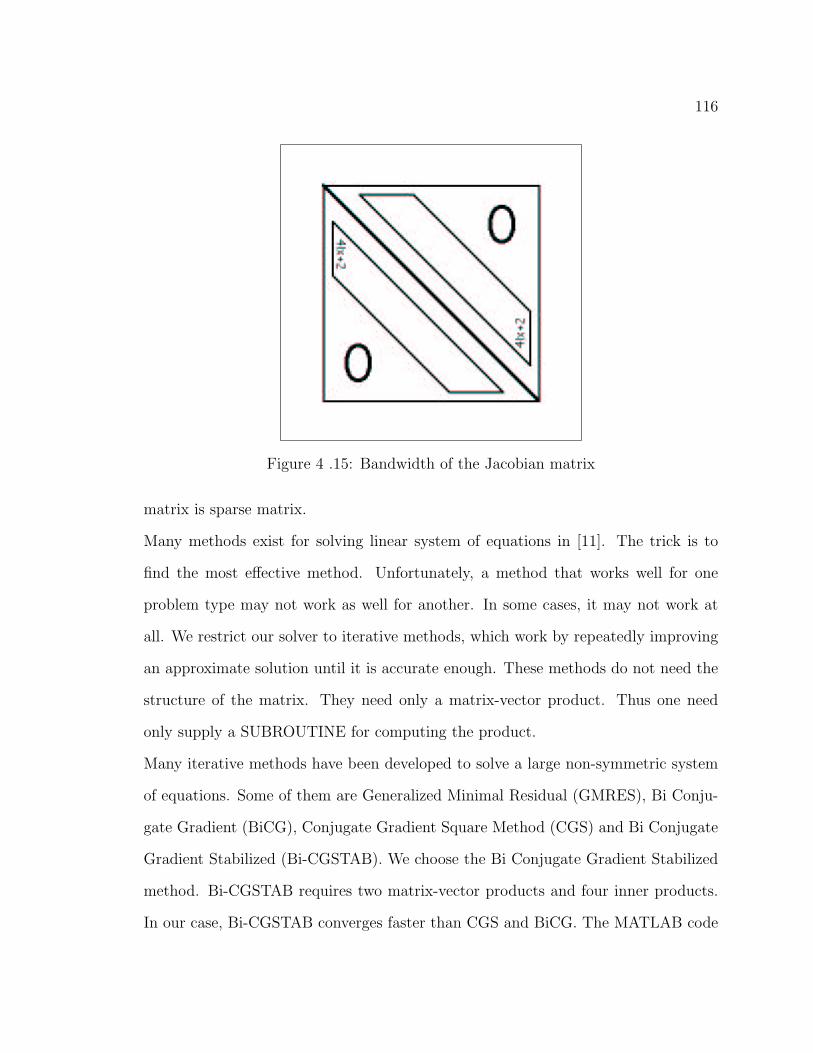
116
Figure 4 .15: Bandwidth of the Jacobian matrix
matrix is sparse matrix.
Many methods exist for solving linear system of equations in [11]. The trick is to
find the most effective method. Unfortunately, a method that works well for one
problem type may not work as well for another. In some cases, it may not work at
all. We restrict our solver to iterative methods, which work by repeatedly improving
an approximate solution until it is accurate enough. These methods do not need the
structure of the matrix. They need only a matrix-vector product. Thus one need
only supply a SUBROUTINE for computing the product.
Many iterative methods have been developed to solve a large non-symmetric system
of equations. Some of them are Generalized Minimal Residual (GMRES), Bi Conju-
gate Gradient (BiCG), Conjugate Gradient Square Method (CGS) and Bi Conjugate
Gradient Stabilized (Bi-CGSTAB). We choose the Bi Conjugate Gradient Stabilized
method. Bi-CGSTAB requires two matrix-vector products and four inner products.
In our case, Bi-CGSTAB converges faster than CGS and BiCG. The MATLAB code
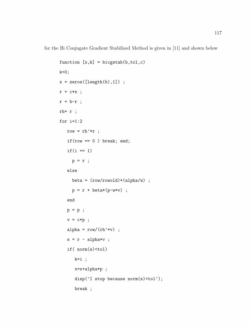
117
for the Bi Conjugate Gradient Stabilized Method is given in [11] and shown below
function [x,k] = bicgstab(b,tol,c)
k=0;
x = zeros([length(b),1]) ;
r = c*x ;
r = b-r ;
rh= r ;
for i=1:2
row = rh’*r ;
if(row == 0 ) break; end;
if(i == 1)
p = r ;
else
beta = (row/rowold)*(alpha/w) ;
p = r + beta*(p-w*v) ;
end
p = p ;
v = c*p ;
alpha = row/(rh’*v) ;
s = r - alpha*v ;
if( norm(s)<tol)
k=i ;
x=x+alpha*p ;
disp(’I stop because norm(s)<tol’);
break ;
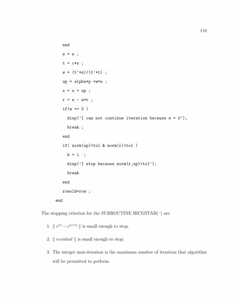
118
end
s = s ;
t = c*s ;
w = (t’*s)/(t’*t) ;
up = alpha*p +w*s ;
x = x + up ;
r = s - w*t ;
if(w == 0 )
disp(’I can not continue iteration because w = 0’);
break ;
end
if( norm(up)<tol & norm(r)<tol )
k = i ;
disp(’I stop because norm(r,up)<tol’);
break
end
rowold=row ;
end
The stopping criterion for the SUBROUTINE BICGSTAB(–) are
1. ‖ c(i) − c(i+1) ‖ is small enough to stop.
2. ‖ residual ‖ is small enough to stop.
3. The integer max-iteration is the maximum number of iteration that algorithm
will be permitted to perform.

119
4.14 COARSE-LEVEL-SOLVE Subroutine
In the main program, we call SUBROUTINE MAELNODE (–) which generate the
geometry information. It returns ielnode vector which represents the information
about the global node ordering and it returns ibo vector which has information about
the boundary node. Then we call COORD(–) SUBROUTINE which return xx-vector
and yy-vector which have the x-coordinate and y-coordinate of each node. Then we
call MAEA(–) SUBROUTINE which returns the elements stiffness matrix. Then we
call quad7(–) SUBROUTINE which returns the abscissa and the weight for numerical
integration formula. Then it calls PHIQ(–) SUBROUTINE which returns the function
values, the x-derivative and the y-derivative of the reference element basis functions
at the integration points. Then it calls MAB(–) SUBROUTINE which returns the
element 3-dimentional array B.
After all these SUBROUTINE calls, COARSE-LEVEL-SOLVE SUBROUTINE is
called to compute, ψH , an approximation of the streamfunction on the coarse mesh.
Inside the coarse-level-solver SUBROUTINE we start Newton’s iteration. In each
iteration we make 5 calls to 5 SUBROUTINES until we satisfy the shopping criteria.
First call is JACOB(–) SUBROUTINE which compute the Jacobian . Then we call
FORCE(–) SUBROUTINE to compute rhs-vector. Then we call BOUNDARY-A(–)
and BOUNDARY RHS(–) SUBROUTINES to take care of the boundary conditions.
The last call is BICGSTAB(–) which will solve the linear system.
4.15 FINE-LEVEL-SOLVE Subroutine
Here we consider the implementation of the two level element method for one level
formulation. After we compute the approximate solution ψH in the coarse mesh, we

120
have to compute ψh on the fine mesh. For specificity, consider the following problem,
solve the linear system on fine mesh for ψh ∈ Xh,
a(ψh, φh) + b(ψH , ψh, φh) = (f, curl φh) for all φh ∈ Xh. (4 .28)
Here,
a(ψh, φh) =∑
l
∫
ei
(ψhxxφ
hxx + 2ψh
xyφhxy + ψh
yyφhyy)dxdy,
b(ψH , ψh, φh) =∑
l
∫
ei
(ψHy ψh
xx − ψHx ψh
xy)φhx − (ψH
x ψhyy − ψH
y ψhxy)φ
hydxdy.
(4 .29)
The solution of the above equation requires
1. generating the fine mesh.
2. the assembly of the linear system.
3. the solution of the resulting linear system.
To generate the fine mesh, one input a new lx number into the SUBROUTINE
MAELNODE(–) and COORD(–). Then, SUBROUTINE MAELNODE(–) and SUB-
ROUTINE COORD(–) will generate ielnode array, ibo vector, xx-vector and yy-
vector for the new mesh. The ielnode array has a global node label map for all
elements for the new mesh. The ibo-vector contains the boundary number. xx-vector
and yy-vector have the x-coordinate and y-coordinate of all nodes.
To complete item (2), we need to assemble the matrix Aand the rhs of the linear
system. To assemble the matrix A, we have to compute the value of ψH on the new
nodes because the values of ψH is only known at the coarse mesh nodes.
Let φhi : i = 1, . . . , mh denote the global basis functions, defined on ~Ωh. We want
to approximate ψ(x, y) by a function ψh in the space Sh = spanφhi : i = 1, . . . , mh.
121
As ψh(x, y) lies in Sh we may expand:
ψh(x, y) =
mh∑i=1
cjφhj (x, y). (4 .30)
Now, the problem is computing the coefficients cj’s in ( 4 .30). Taking the variation
of ( 4 .28) over Sh given the variational equations which ψh(x, y) satisfies:
a(ψh, φh) + b(ψH , ψh, φh) = (f, curl φh) for all φh ∈ Sh. (4 .31)
Setting φh = φhi (x, y) in ( 4 .31) and substituting ( 4 .30) yields
mh∑j=1
cja(φhj , φ
hi ) +
mh∑j=1
cjb(ψH , φh
j , φhi ) = (f, curl φh
i ) i = 1, . . . , m . (4 .32)
We assemble b(ψH , φhj , φ
hi ) element by element as
b(ψH , φhj , φ
hi ) =
nelemh∑
l=1
b(l)(ψH , φhj , φ
hi ). (4 .33)
Now, the triangle el is inside a bigger triangle g which is an element of the coarse
mesh, as shown in Figure ( 4 .16).
Hence, we have
ψH =6∑
k=1
dkφ(H)k , (4 .34)
where φ(H)1 , . . . , φ
(H)6 are the local basis functions of the triangle g. d1, d2 and d3 are
the function values of ψH at the vertices of the triangle g, d4, d5 and d6 are the normal
derivatives values of ψH at the midsides points of the triangle g.
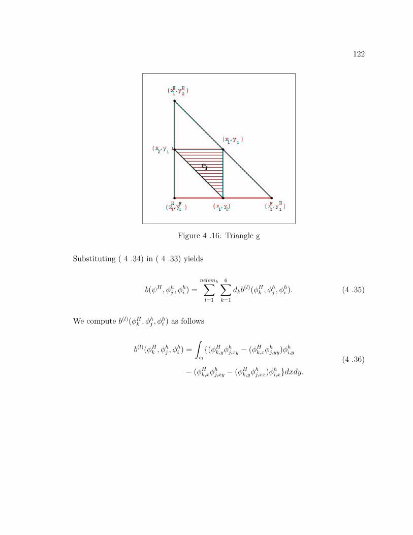
122
Figure 4 .16: Triangle g
Substituting ( 4 .34) in ( 4 .33) yields
b(ψH , φhj , φ
hi ) =
nelemh∑
l=1
6∑
k=1
dkb(l)(φH
k , φhj , φ
hi ). (4 .35)
We compute b(l)(φHk , φh
j , φhi ) as follows
b(l)(φHk , φh
j , φhi ) =
∫
el
(φHk,yφ
hj,xy − (φH
k,xφhj,yy)φ
hi,y
− (φHk,xφ
hj,xy − (φH
k,yφhj,xx)φ
hi,xdxdy.
(4 .36)

123
By chain rule calculation we have
φhx =
1
x2 − x1
φξ =1
hφξ,
φhy =
1
y3 − y1
φη =1
hφη,
φhxy =
1
(x2 − x1)(y3 − y1)φξη =
1
h2φξη,
φhxx =
1
(x2 − x1)2φξξ =
1
h2φξξ, (4 .37)
φhyy =
1
(y3 − y1)2φηη =
1
h2φηη,
φHk,x =
1
(xH2 − xH
1
φξ =1
Hφξ,
φHk,y =
1
(yH3 − yH
1
φη =1
Hφη.
Substituting ( 4 .37) in ( 4 .36) yields
b(l)(φHk , φh
j , φhi ) =
∫
e
( φk,η
H
φj,ξη
h2− φk,ξ
H
φj,ξη
h2)φi,η
h
− (φk,ξ
H
φj,ξη
h2− φk,η
H
φj,ξξ
h2)φi,ξ
hh2dξdη,
=1
Hh
∫
e
(φk,ηφj,ξη − φk,ξφj,ηη)φi,η
− (φk,ξφj,ξη − φk,ηφj,ξξ)φi,ξdξdη,
=1
Hhb(i)jk . (4 .38)
Hence, using ( 4 .35) and ( 4 .38) gives
b(ψH , φhj , φ
hi ) =
nelemh∑
l=1
6∑
k=1
dk
Hhb(i)jk
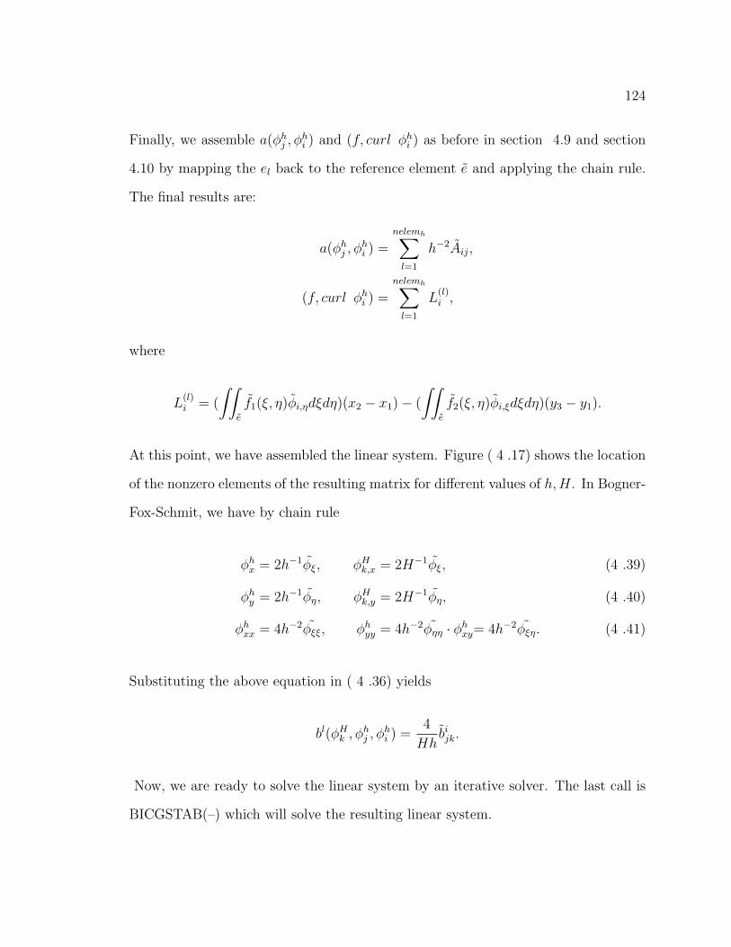
124
Finally, we assemble a(φhj , φ
hi ) and (f, curl φh
i ) as before in section 4.9 and section
4.10 by mapping the el back to the reference element e and applying the chain rule.
The final results are:
a(φhj , φ
hi ) =
nelemh∑
l=1
h−2Aij,
(f, curl φhi ) =
nelemh∑
l=1
L(l)i ,
where
L(l)i = (
∫∫
e
f1(ξ, η)φi,ηdξdη)(x2 − x1)− (
∫∫
e
f2(ξ, η)φi,ξdξdη)(y3 − y1).
At this point, we have assembled the linear system. Figure ( 4 .17) shows the location
of the nonzero elements of the resulting matrix for different values of h, H. In Bogner-
Fox-Schmit, we have by chain rule
φhx = 2h−1φξ, φH
k,x = 2H−1φξ, (4 .39)
φhy = 2h−1φη, φH
k,y = 2H−1φη, (4 .40)
φhxx = 4h−2φξξ, φh
yy = 4h−2φηη · φhxy= 4h−2φξη. (4 .41)
Substituting the above equation in ( 4 .36) yields
bl(φHk , φh
j , φhi ) =
4
Hhbijk.
Now, we are ready to solve the linear system by an iterative solver. The last call is
BICGSTAB(–) which will solve the resulting linear system.
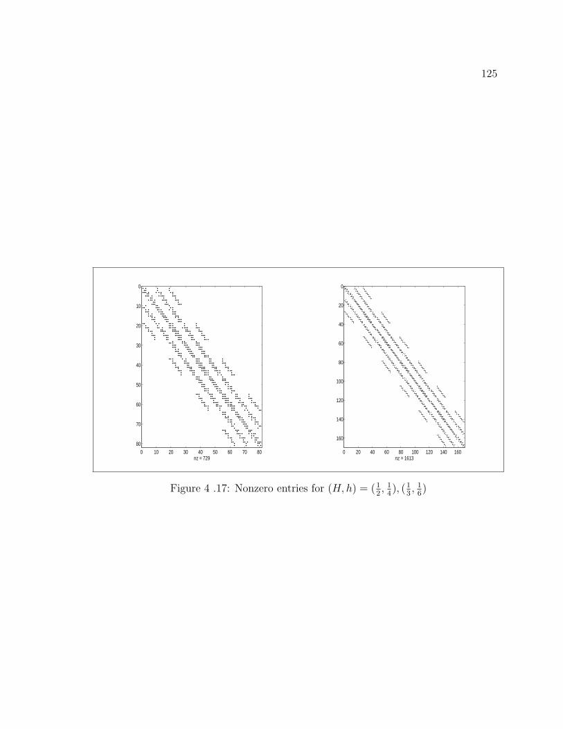
125
0 10 20 30 40 50 60 70 80
0
10
20
30
40
50
60
70
80
nz = 7290 20 40 60 80 100 120 140 160
0
20
40
60
80
100
120
140
160
nz = 1613
Figure 4 .17: Nonzero entries for (H, h) = (12, 1
4), (1
3, 1
6)

Chapter 5
Numerical Tests
126

127
5.1 Introduction
Although the theoretical result in chapter ( 2 ) looks quite nice it has an essential
drawback from the practical point of view. There are several open questions left from
theory. How does the constant C in the estimate ( 2 .23) depend on the Reynolds
number Re and how do the error norms ‖ ψ−ψh ‖h behave if we keep the mesh sizes
H and h fixed and increase Re? How much time in practical settings we save when
we use a two level method instead of a one level method? Will the solution’s quality
differ in using the two level method instead of the one level method?
In section ( 5.2) we test the code described in chapter ( 2 ) with problems which
have a known solution to compare one level vs. two level methods. Section ( 5.3)
contains the graphs of the test problem with known solution with different values of
Reynolds numbers. This problem have been tested in [63] with Re = 10, 50, 100, 1000
and 2000. In section ( 5.5) we solve the driven cavity problems. These flows have been
widely used as test cases for validating incompressible fluid dynamics algorithms. We
will compare our streamlines with the streamlines in [31, 2].
5.2 Accuracy Two Level Method vs. One Level
Method
We consider as a test example the 2D Navier-Stokes problem as the unit square
Ω = [0, 1]2 where we define the right hand side by
f := − 1
Re4 u + (u · 5)u +5p,

128
with the following prescribed exact solution
u =
ψy
ψx
,
ψ(x, y) = x2(x− 1)2y2(y − 1)2,
p(x, y) = x3 + y3 − 0.5 .
For this test problem, all requirements of the theory concerning the geometry of the
domain and the smoothness of the data are satisfied. Moreover, the streamfunction
ψ(x, y) satisfies the boundary conditions of the streamfunction equation of the Navier-
Stokes equation (i.e)
ψ(x, y) = 0 where x = 0, x = 1, y = 0, or y = 1, (5 .1)
∂ψ(x, y)
∂n= 0 where x = 0, x = 1, y = 0, or y = 1. (5 .2)
Also the exact solution is very smooth and does not depend on the Reynolds number.
Our goal in this test is to validate the code and the properties and merits of the
two level method as compared with the one level method. In all numerical calcu-
lations in this section we have used the Bogner-Fox-Schmit elements with Re = 10
and tol = 10−3. We pick three values of h. They are 18, 1
14and 1
16. All the compu-
tations in this section are done using 133Mhz Intel Pentium Processor with 32 MHz
Ram running Windows NT. The cpu-time, number of Newton’s iterations, number of
Bicgstab iterations, the L2-error, H1-error and H2-error of the streamfunction ψ for
the one level method for different values of h are tabulated in Table ( 5 .1). Table
( 5 .2) shows cpu-time, number of Newton’s iterations and the number of Bicgstab’s
iterations for each linear solver for two level method. Figure ( 5 .1) shows, for fixed

129
Re = 10 using one level method, the streamlines for h = 18, 1
14, 1
16and the correspond-
ing three-dimensional plot of the streamfunction ψ(x, y).
Remarks 1
1. From Table( 5 .1) and Table( 5 .2), the cpu-time for two level method is much
smaller than the corresponding cpu-time for one level method. For h = 18, 1
14,
we save about 57%. For h = 116
we save about 73%. For example, in h = 116
we
need to solve a nonlinear system of 1156 equations which requires solving three
linear systems of equations of order 1156. The corresponding two level method
requires solving a nonlinear system of 324 equations and a linear system of 1156
equations. We anticipate the savings to increase as the mesh is further refined.
2. From Figure ( 5 .1) and Figure ( 5 .2) both graphs are exactly similar, which
means that the two level method produces a solution with the same quality as
the one level method.
3. From Table ( 5 .1) and Table ( 5 .2) both H1-error and H2-error are of the same
order, which means that the velocity field is of the same error and quality in
both methods since u = ψy and v = −ψx.
4. From Table ( 5 .1) and Table ( 5 .2) L2-error of the one level method table is
somewhat better than the L2-error of the two level method table.
5. In this test we used the approximate solution produced from step 1 in assembling
the matrix of step 2. We used the zero vector as an initial guess for solving the
linear system of step 2.
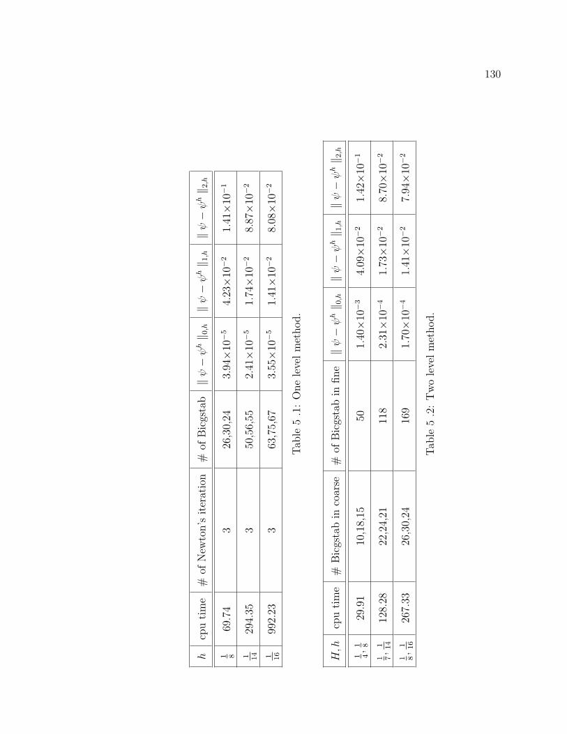
130
hcp
uti
me
#of
New
ton’s
iter
atio
n#
ofB
icgs
tab
‖ψ−
ψh‖ 0
,h‖ψ
−ψ
h‖ 1
,h‖ψ
−ψ
h‖ 2
,h
1 869
.74
326
,30,
243.
94×1
0−5
4.23×1
0−2
1.41×1
0−1
1 14
294.
353
50,5
6,55
2.41×1
0−5
1.74×1
0−2
8.87×1
0−2
1 16
992.
233
63,7
5,67
3.55×1
0−5
1.41×1
0−2
8.08×1
0−2
Tab
le5
.1:
One
leve
lm
ethod.
H,h
cpu
tim
e#
Bic
gsta
bin
coar
se#
ofB
icgs
tab
infine
‖ψ−
ψh‖ 0
,h‖ψ
−ψ
h‖ 1
,h‖ψ
−ψ
h‖ 2
,h
1 4,
1 829
.91
10,1
8,15
501.
40×1
0−3
4.09×1
0−2
1.42×1
0−1
1 7,
1 14
128.
2822
,24,
2111
82.
31×1
0−4
1.73×1
0−2
8.70×1
0−2
1 8,
1 16
267.
3326
,30,
2416
91.
70×1
0−4
1.41×1
0−2
7.94×1
0−2
Tab
le5
.2:
Tw
ole
velm
ethod.

131
1 2 3 4 5 6 7 8 91
2
3
4
5
6
7
8
9
0.00371
0.00352
0.00273
0.00195
0.00117
0.000391
7.03e−005
02
46
810
0
2
4
6
8
100
0.5
1
1.5
2
2.5
3
3.5
4
x 10−3
2 4 6 8 10 12 14
2
4
6
8
10
12
14
0.00371
0.00352
0.00273
0.00195
0.00117
0.000391
7.03e−0053.91e−008
0
5
10
15
0
5
10
150
0.5
1
1.5
2
2.5
3
3.5
4
x 10−3
2 4 6 8 10 12 14 16
2
4
6
8
10
12
14
16
7.03e−005
0.000391
0.00117
0.00195
0.00273
0.00352
0.00371
3.91e−008
0
5
10
15
20
0
5
10
15
200
0.5
1
1.5
2
2.5
3
3.5
4
x 10−3
Figure 5 .1: Streamlines for h = 18, 1
14, 1
16with Re=10 and the corresponding 3-D
graphs using one level method
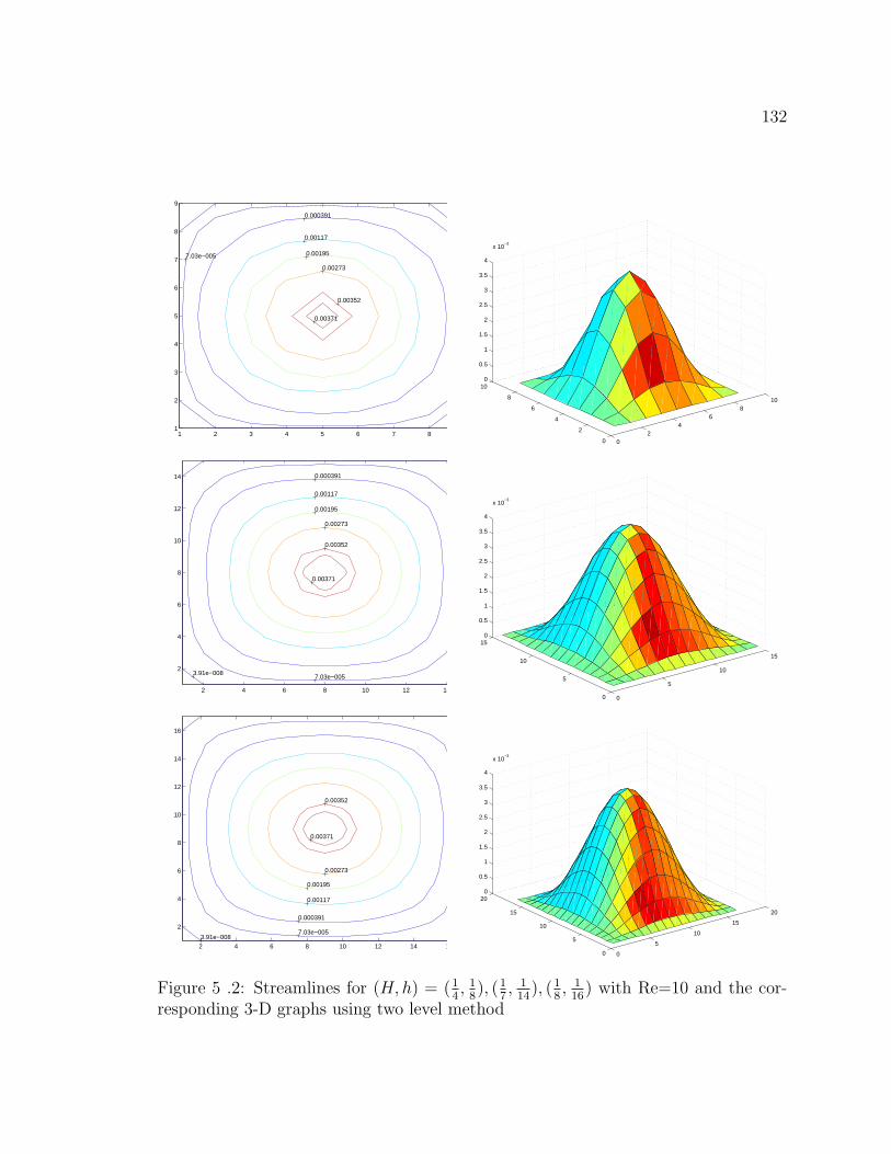
132
1 2 3 4 5 6 7 8 91
2
3
4
5
6
7
8
9
0.00371
0.00352
0.00273
0.00195
0.00117
0.000391
7.03e−005
02
46
810
0
2
4
6
8
100
0.5
1
1.5
2
2.5
3
3.5
4
x 10−3
2 4 6 8 10 12 14
2
4
6
8
10
12
14
0.00371
0.00352
0.00273
0.00195
0.00117
0.000391
7.03e−0053.91e−008
0
5
10
15
0
5
10
150
0.5
1
1.5
2
2.5
3
3.5
4
x 10−3
2 4 6 8 10 12 14 16
2
4
6
8
10
12
14
16
7.03e−005
0.000391
0.00117
0.00195
0.00273
0.00352
0.00371
3.91e−008
0
5
10
15
20
0
5
10
15
200
0.5
1
1.5
2
2.5
3
3.5
4
x 10−3
Figure 5 .2: Streamlines for (H, h) = (14, 1
8), (1
7, 1
14), (1
8, 1
16) with Re=10 and the cor-
responding 3-D graphs using two level method
133
5.3 Robustness: Test Problem for Different Reynolds
Numbers
In this section, we consider the example which was described in the previous section.
The exact solution is very smooth and does not depend on the Reynolds number.
The point of these tests is to increase the Reynolds number with h fixed and test
the robustness of the method. Schieweck [63] tested his code with this problem.
He used two nonconforming finite element approximations of upwind type for the
velocity-pressure formulation. Our goal in this test is to determine the validation of
the code and the norm behavior when Re is varying and compare our streamlines
with Schieweck’s streamlines.
The numerical computations of this section was obtained using a Sun Ultra 2 with
2 200Mhz ultrasparc processors running Solaris 2.5.1 . In all numerical calculations,
we used the Bogner-Fox-Schmit rectangles and Morley triangles. The streamlines for
Re = 10, 50, 100, 200, 1000 and 2000 were obtained with 17× 17 grid points on the
coarse mesh and 33 × 33 grid on the fine mesh. Hence, a mesh of 256 elements and
a mesh of 1024 elements were used in this test for the case of Bogner-Fox-Schmit
rectangles. In Morley elements, a mesh of 512 elements and a mesh of 2048 elements
were used.
The initial guess in solving the nonlinear system of equation on the coarse mesh
was the zero vector or the zero function except the cases where Re = 200, 1000 and
2000. In this case the one level method with the choice of initial guess with the
same tolerance failed. So we used the first iterates of the Newton’s method when we
solve the problem with Re = 100 as the initial guess for these cases. The number
of Bicgstab steps needed for converging the linear system in the fine mesh and the
number of Bicgstab steps needed for solving the nonlinear system of equations in
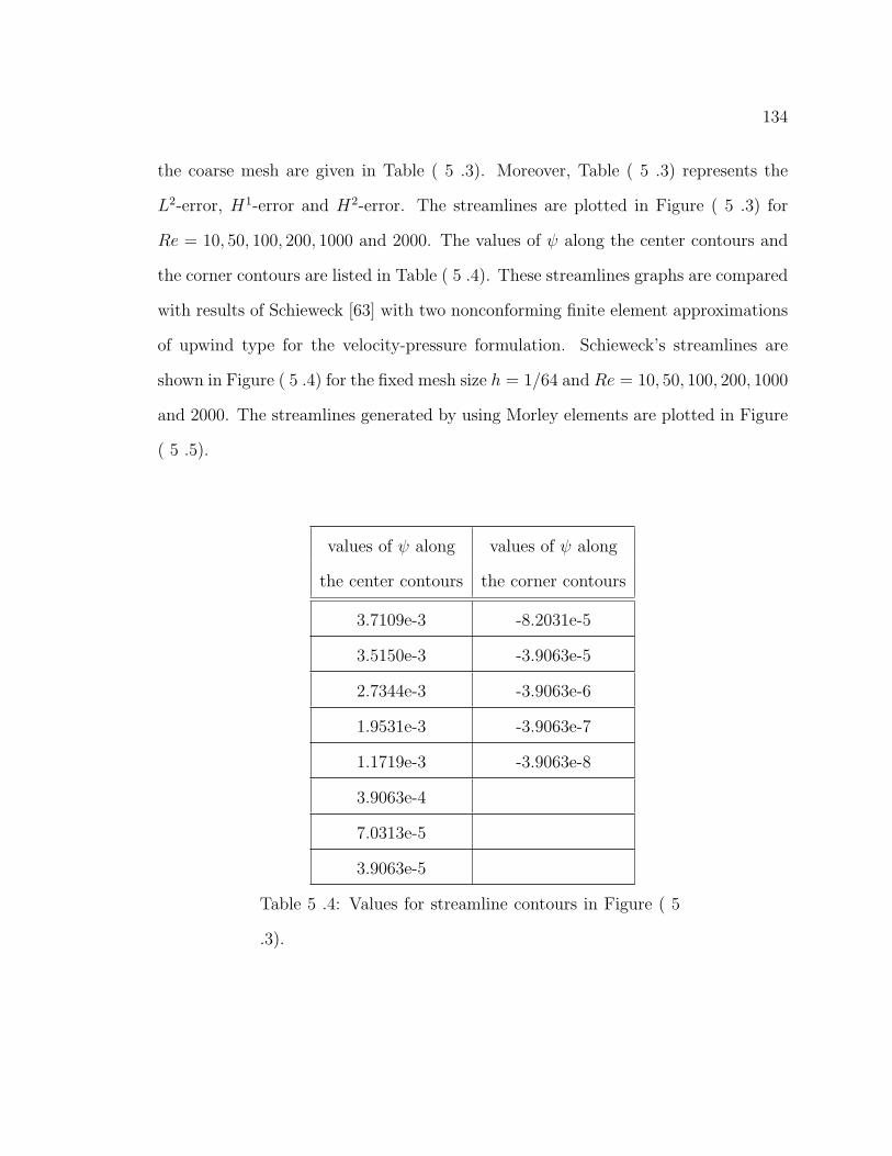
134
the coarse mesh are given in Table ( 5 .3). Moreover, Table ( 5 .3) represents the
L2-error, H1-error and H2-error. The streamlines are plotted in Figure ( 5 .3) for
Re = 10, 50, 100, 200, 1000 and 2000. The values of ψ along the center contours and
the corner contours are listed in Table ( 5 .4). These streamlines graphs are compared
with results of Schieweck [63] with two nonconforming finite element approximations
of upwind type for the velocity-pressure formulation. Schieweck’s streamlines are
shown in Figure ( 5 .4) for the fixed mesh size h = 1/64 and Re = 10, 50, 100, 200, 1000
and 2000. The streamlines generated by using Morley elements are plotted in Figure
( 5 .5).
values of ψ along values of ψ along
the center contours the corner contours
3.7109e-3 -8.2031e-5
3.5150e-3 -3.9063e-5
2.7344e-3 -3.9063e-6
1.9531e-3 -3.9063e-7
1.1719e-3 -3.9063e-8
3.9063e-4
7.0313e-5
3.9063e-5
Table 5 .4: Values for streamline contours in Figure ( 5
.3).

135
Re
(H,h
)#
Bic
gsta
bin
coar
se#
ofB
icgs
tab
infine
‖ψ−
ψh‖ 0
,h‖ψ
−ψ
h‖ 1
,h‖ψ
−ψ
h‖ 2
,h
10(
1 16,
1 32)
61,6
6,43
576
4.21×1
0−5
4.84×1
0−3
5.27×1
0−2
50(
1 16,
1 32)
54,8
3,17
3,29
2,82
1676
1.11×1
0−4
4.82×1
0−3
5.19×1
0−2
100
(1 16,
1 32)
53,2
54,4
21,6
68,1
287
4356
4.44×1
0−4
5.00×1
0−3
5.11×1
0−2
200
(1 16,
1 32)
53,2
54,4
21,6
68,1
287,
454
4356
3.06×1
0−4
4.52×1
0−3
5.07×1
0−2
1000
(1 16,
1 32)
53,2
54,4
21,6
68,1
287,
1156
4356
9.62×1
0−4
1.08×1
0−2
1.83×1
0−1
2000
(1 16,
1 32)
53,2
54,4
21,6
68,1
287,
1156
,115
6,11
5643
561.
93×1
0−3
2.59×1
0−2
4.93×1
0−1
Tab
le5
.3:
Tw
ole
velfo
rte
stpro
ble
m.

136
5 10 15 20 25 30
5
10
15
20
25
30
0.00371
0.00352
0.00273
0.00195
0.00117
0.000391
7.03e−005
3.91e−008
(a) Exact
5 10 15 20 25 30
5
10
15
20
25
30
0.00371
0.00352
0.00195
0.00117
7.03e−005
3.91e−008
(b) Re=10
5 10 15 20 25 30
5
10
15
20
25
30
0.00371
0.00352
0.00273
0.00195
0.00117
0.0003917.03e−005
3.91e−008
(c) Re=50
5 10 15 20 25 30
5
10
15
20
25
30
0.00371
0.00352
0.00273
0.00195
0.00117
0.0003917.03e−005
3.91e−008
(d) Re=100
5 10 15 20 25 30
5
10
15
20
25
30
0.0037109
0.0035156
0.0027344
0.0019531
0.0011719
0.000390627.0312e−005
3.9062e−008
−3.9062e−008
(e) Re=1000
5 10 15 20 25 30
5
10
15
20
25
30
0.0037109
0.0035156
0.0027344
0.0019531
0.0011719
0.00039062
7.0312e−005
−3.9062e−005
−3.9062e−007
(f) Re=2000
Figure 5 .3: Streamlines for H = 116
, h = 132
using Bogner-Fox-Schmit element.

137
Figure 5 .4: Streamlines for h = 164
(courtesy F. Schieweck [63]).

138
5 10 15 20 25 30
5
10
15
20
25
30
0.00371
0.00352
0.00273
0.00195
0.00117
0.000391
7.03e−005
3.91e−008
(a) Exact
10 20 30 40 50 60
10
20
30
40
50
60
−2.5e−0060.0001
0.00055
0.001
0.0015
0.0019
(b) Re=10
5 10 15 20 25 30
5
10
15
20
25
30
0.0024
0.002
0.0015
0.001
0.00055
0.0001
−2e−005−0.00022
−0.0004
−2e−005−0.0004
−0.00022
(c) Re=50
5 10 15 20 25 30
5
10
15
20
25
30
0.003
0.00150.001
0.00055
0.0001
−0.0004
−0.001
−0.001
−0.0004
−2e−005
(d) Re=100
Figure 5 .5: Streamlines for H = 116
, h = 132
using Morley element.

139
Remarks 2
1. Figures ( 5 .3, 5 .4, 5 .5) show that the increasing in the Reynolds number will
affect the streamlines.
2. Figure ( 5 .3) shows increasing in Reynolds number will increase the number of
corner contours.
3. Figure ( 5 .3) shows better quality of the solutions if they are compared to
Figure ( 5 .4) and ( 5 .5). This has two explanations. Firstly, the use of high
order polynomials. In Bogner-Fox-Schmit, the polynomial is bicubic. Secondly,
the use of conforming elements will decrease the error.
4. From Table ( 5 .3), H2-error and H1-error are of the same order. However,
increasing the Reynolds number will effect the L2-error.
5.4 Meshes Scaling Test
The error between the coarse and fine meshes are related superlinearly via:
| ψ − ψh |2≤ C infwh∈Xh
| ψ − wh |2 + | ln h |1/2 · | ψ − ψH |1.
If the Bogner-Fox-Schmit rectangles are used, then the coarse and fine meshes are
related by
h = O(H3/2 | ln H |1/4). (5 .3)
In this section, we will test the scaling ( 5 .3) by fixing H = 14. From equation ( 5
.3), the computed values of h is 17
or 18. The idea here is how much can we reduce the
value of h, and how well the quality of the solution be. For this purpose, we consider
140
the example in section ( 5.2). In all numerical calculations in this section, we have
used the Bogner-Fox-Schmit elements with Re = 100 and tol = 10−6.
We pick four pairs of (H, h). They are (14, 1
8), (1
4, 1
8), (1
4, 1
16) and (1
4, 1
20). All the
computations in this section are done using 133 MHz Intel Pentium processor with 32
MHz Ram running Windows NT. The L2-error, H1-error and H2-error of the stream-
function ψ these four pairs of (H, h) are tabulated in Table ( 5 .5). Figure ( 5 .6)
shows the streamlines for (H, h) = (14, 1
8), (1
4, 1
8), (1
4, 1
16) and (1
4, 1
20).
Remark 1
Table ( 5 .5) shows that the error norms increase if we keep the coarse mesh size fixed
and decrease the fine mesh size. This effect can be seen more clearly in Figure ( 5 .6).
Figure ( 5 .6) shows that the number of negative streamlines increases if we decrease
the fine mesh size h. One explanation for this effect is due to the error bound of this
problem, namely,
| ψ − ψh |≤ C1h2 + C2
√| ln h |H3 where C2 > C1.
If we decrease the fine mesh size h then the first term in the above error biund
decreases. However, the second term increases and hence it becomes the dominate
term. To get the optimum value for h one may need to balance between these two
terms. The error bounds for all four cases are given below.

141
| ψ − ψh |2≤ C1(0.0156) +C2(0.0225) for (H, h) = (1
4,1
8),
| ψ − ψh |2≤ C1(0.00694)+C2(0.0246) for (H, h) = (1
4,
1
12),
| ψ − ψh |2≤ C1(0.00391) +C2(0.026) for (H, h) = (1
4,
1
16),
| ψ − ψh |2≤ C1(0.0025) +C2(0.027) for (H, h) = (1
4,
1
20).
Re (H,h) ‖ ψ − ψh ‖0,h ‖ ψ − ψh ‖1,h ‖ ψ − ψh ‖2,h
100 (14, 1
8) 5.53×10⁻⁸ 2.37×10⁻⁵ 9.89×10⁻⁵
100 (14, 1
12) 2.83×10⁻⁷ 2.52×10⁻⁵ 1.09×10⁻⁴
100 (14, 1
16) 1.14×10⁻⁷ 2.59×10⁻⁵ 1.13×10⁻⁴
100 (14, 1
20) 3.41×10⁻⁷ 2.65×10⁻⁵ 1.16×10⁻⁴
Table 5 .5: L2-error, H1-error and H2-error of ψ for dif-
ferent pairs (H, h).
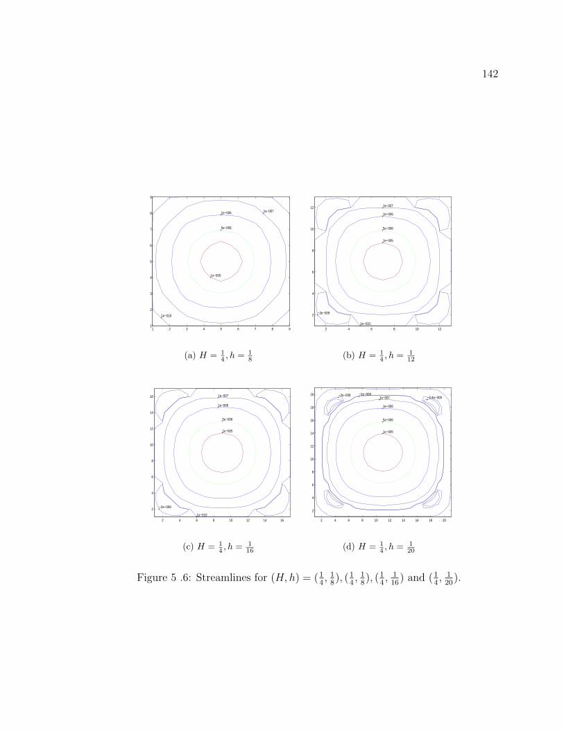
142
1 2 3 4 5 6 7 8 91
2
3
4
5
6
7
8
9
1e−005
5e−006
1e−006 1e−007
1e−010
(a) H = 14 , h = 1
8
2 4 6 8 10 12
2
4
6
8
10
12
1e−005
5e−006
1e−006
1e−007
1e−010
−2e−009
(b) H = 14 , h = 1
12
2 4 6 8 10 12 14 16
2
4
6
8
10
12
14
16
1e−005
5e−006
1e−006
1e−007
1e−010
−2e−009
(c) H = 14 , h = 1
16
2 4 6 8 10 12 14 16 18 20
2
4
6
8
10
12
14
16
18
20
1e−005
5e−006
1e−006
1e−007−2e−009−2e−008
−2.4e−008
(d) H = 14 , h = 1
20
Figure 5 .6: Streamlines for (H, h) = (14, 1
8), (1
4, 1
8), (1
4, 1
16) and (1
4, 1
20).
143
5.5 The Driven Cavity Problem
Cavity flows have been a subject of study for some time. These flows have been
widely used as test cases for validating incompressible fluid dynamics algorithms.
Corner singularities for two-dimensional fluid flows are very important, since most
examples of physical interest have corners. For example, singularities of most elliptic
problems develop when the boundary contour is not smooth. In this section, we
will study the driven flow in a rectangular cavity when the top surface moves with a
constant velocity along its length. The upper corners where the moving surface meets
the stationary walls are singular points of the flow at which the horizontal velocity is
multi-valued. The lower corners are also weakly singular points.
We consider a domain Ω = [0, 1] × [0, 1] with no-slip boundary conditions, i.e,
u = v = 0 in all boundaries except y = 1 where u = 1. This problem have been
studied and addressed by many researchers including Ghia, Ghia, Shin [31], J.E Akin
[2] and Betts-Haroutunian [12]. Ghia’s algorithm is based on the time dependent
streamfunction equation using a multi grid technique. The numerical computational
in this section was obtained using a Sun Ultra 2 with 2 200 MHz ultrasparc processors
running Solaris 2.5.1 . Bogner-Fox-Schmit elements are used with 17× 17 grid points
on the coarse mesh and 33 × 33 grid points on the fine mesh. The streamlines for
Re = 1, 10, 50 and 100 are plotted in Figure ( 5 .7, 5 .8). These results are compared
with results of Ghia [31] obtained with 129 × 129 grid. Moreover, these results are
illustrated with Akin’s streamlines in Figure ( 5 .9). Table ( 5 .6) and Table ( 5 .7) list
the numerical values corresponding to the velocity profiles for lines passing through
the geometric center of the cavity. Table ( 5 .8) represents the number of Bicgstab
steps in coarse mesh and the number of Bicgstab steps in the fine mesh.
144
Remarks 3
1. From Figure ( 5 .9), good agreement can be found in the case of Re = 1.
2. Good agreement can be found between the case of Re = 1, 10 in Figure ( 5 .7)
and the case of Re = 100, 400 in Figure ( 5 .8). Moreover, The corresponding
u-velocity and v-velocity agree, too Figure ( 5 .10).
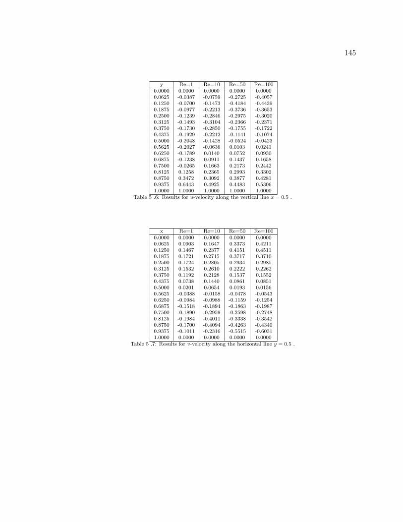
145
y Re=1 Re=10 Re=50 Re=1000.0000 0.0000 0.0000 0.0000 0.00000.0625 -0.0387 -0.0759 -0.2725 -0.40570.1250 -0.0700 -0.1473 -0.4184 -0.44390.1875 -0.0977 -0.2213 -0.3736 -0.36530.2500 -0.1239 -0.2846 -0.2975 -0.30200.3125 -0.1493 -0.3104 -0.2366 -0.23710.3750 -0.1730 -0.2850 -0.1755 -0.17220.4375 -0.1929 -0.2212 -0.1141 -0.10740.5000 -0.2048 -0.1428 -0.0524 -0.04230.5625 -0.2027 -0.0636 0.0103 0.02410.6250 -0.1789 0.0140 0.0752 0.09300.6875 -0.1238 0.0911 0.1437 0.16580.7500 -0.0265 0.1663 0.2173 0.24420.8125 0.1258 0.2365 0.2993 0.33020.8750 0.3472 0.3092 0.3877 0.42810.9375 0.6443 0.4925 0.4483 0.53061.0000 1.0000 1.0000 1.0000 1.0000
Table 5 .6: Results for u-velocity along the vertical line x = 0.5 .
x Re=1 Re=10 Re=50 Re=1000.0000 0.0000 0.0000 0.0000 0.00000.0625 0.0903 0.1647 0.3373 0.42110.1250 0.1467 0.2377 0.4151 0.45110.1875 0.1721 0.2715 0.3717 0.37100.2500 0.1724 0.2805 0.2934 0.29850.3125 0.1532 0.2610 0.2222 0.22620.3750 0.1192 0.2128 0.1537 0.15520.4375 0.0738 0.1440 0.0861 0.08510.5000 0.0201 0.0654 0.0193 0.01560.5625 -0.0388 -0.0158 -0.0478 -0.05430.6250 -0.0984 -0.0988 -0.1159 -0.12540.6875 -0.1518 -0.1894 -0.1863 -0.19870.7500 -0.1890 -0.2959 -0.2598 -0.27480.8125 -0.1984 -0.4011 -0.3338 -0.35420.8750 -0.1700 -0.4094 -0.4263 -0.43400.9375 -0.1011 -0.2316 -0.5515 -0.60311.0000 0.0000 0.0000 0.0000 0.0000
Table 5 .7: Results for v-velocity along the horizontal line y = 0.5 .

146
Re
(H,h
)#
Bic
gsta
bin
coar
se#
ofB
icgs
tab
infine
resi
dual
onco
arse
resi
dual
onfine
1(
1 16,
1 32)
176,
192,
181,
136
1055
3.53×1
0−6
9.61×1
0−7
10(
1 16,
1 32)
363,
423,
479,
470,
493
2436
8.00×1
0−7
2.00×1
0−7
50(
1 16,
1 32)
5695
,620
5,66
73,5
885,
5560
3404
82.
93×1
0−6
5.49×1
0−7
100
(1 16,
1 32)
2729
0,26
481,
2483
0,18
283
4356
02.
63×1
0−7
5.26×
10−7
Tab
le5
.8:
Tw
ole
velfo
rca
vity
flow

147
5 10 15 20 25 30
5
10
15
20
25
30
1e−005
−6−5
−3
−2
−1
−0.5
−0.1
−0.01
−0.0011e−005
(a) Re=1
5 10 15 20 25 30
5
10
15
20
25
30
−6.5
−5
−3−2
−0.5
−0.1
−0.01
−0.001
0.02
0.001
(b) Re=10
5 10 15 20 25 30
5
10
15
20
25
30
−5.5
−5
−3.8
−3
−2−0.5
−0.1
0.04
0.1
0.0010.001
0.02
(c) Re=50
5 10 15 20 25 30
5
10
15
20
25
30
−3.8
−3
−2
−1
−0.1−0.010.001
0.015
0.040.001
(d) Re=100
Figure 5 .7: Streamlines for H = 116
, h = 132
with different values of Re numbers usingtwo level method

148
(a) Re=100 (b) Re=400
Figure 5 .8: Ghia-Ghia-Shin’s streamlines, 129× 129, (courtesy U. Ghia [31]).

149
0 5 10 15 20 25 30 350
5
10
15
20
25
30
35
(a) Re=1 (b) Re=1
0 5 10 15 20 25 30 350
5
10
15
20
25
30
35
(c) Re=100 (d) Re=100
Figure 5 .9: (a),(c) Streamlines for cavity flow using two level method, (b),(d) Akin’sstreamlines, a mesh of 40× 40 elements, (courtesy J. Akin [2]).
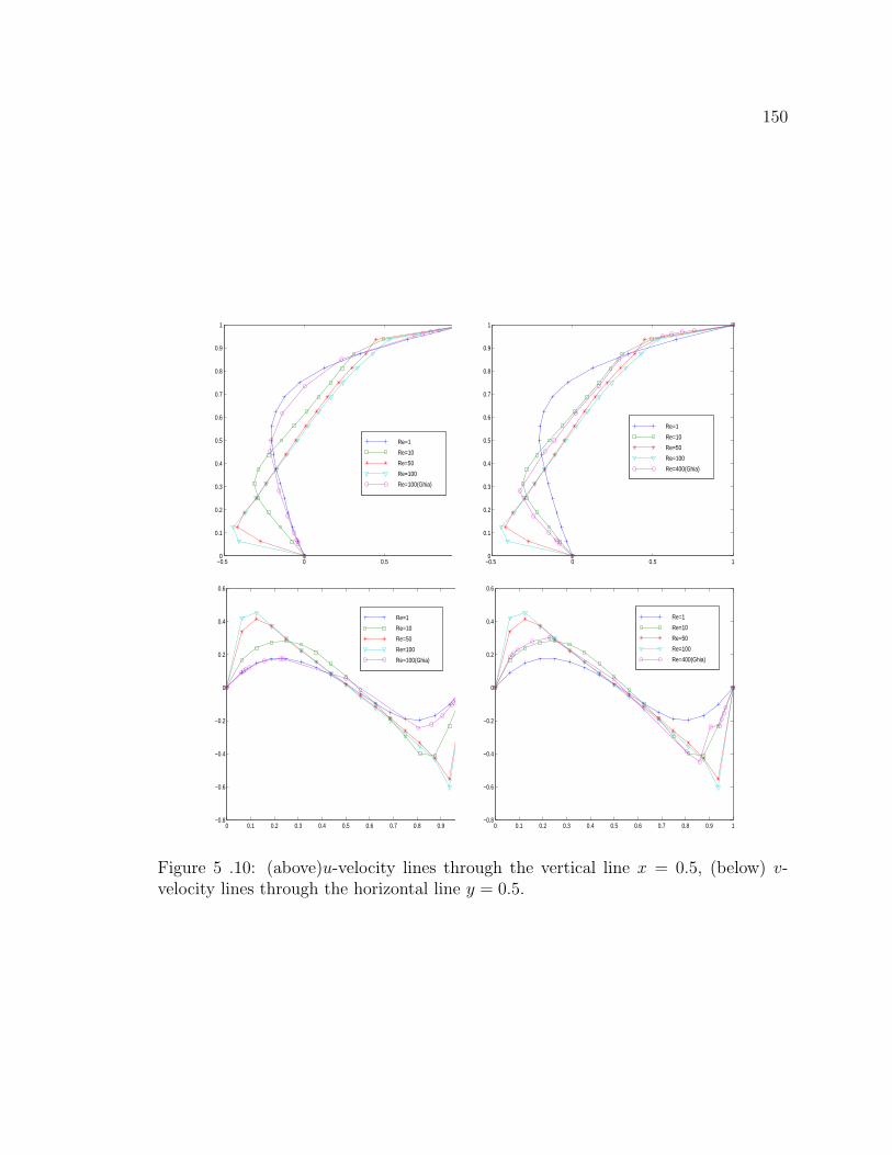
150
−0.5 0 0.5 10
0.1
0.2
0.3
0.4
0.5
0.6
0.7
0.8
0.9
1
Re=1
Re=10
Re=50
Re=100
Re=100(Ghia)
−0.5 0 0.5 10
0.1
0.2
0.3
0.4
0.5
0.6
0.7
0.8
0.9
1
Re=1
Re=10
Re=50
Re=100
Re=400(Ghia)
0 0.1 0.2 0.3 0.4 0.5 0.6 0.7 0.8 0.9 1−0.8
−0.6
−0.4
−0.2
0
0.2
0.4
0.6
Re=1
Re=10
Re=50
Re=100
Re=100(Ghia)
0 0.1 0.2 0.3 0.4 0.5 0.6 0.7 0.8 0.9 1−0.8
−0.6
−0.4
−0.2
0
0.2
0.4
0.6
Re=1
Re=10
Re=50
Re=100
Re=400(Ghia)
Figure 5 .10: (above)u-velocity lines through the vertical line x = 0.5, (below) v-velocity lines through the horizontal line y = 0.5.

Appendix A
FORTRAN 90 Program UsingMorley Element
151

152
PROGRAM FINE_STEP_TEST!--------------------------------------------------! THIS PROGRAM IS FOR SOLVING THE NAVIER-STOKES! EQUATIONS USING THE TWO LEVEL FINITE ELEMENT! METHOD ON THE STREAM FUNCTION FORMULATION! FOR A FULL DESCRIPTION OF THE METHOD SEE! F. FAIRAG, TWO-LEVEL FINITE ELEMENT METHOD! FOR THE STREAM FUNCTION FORMULATION OF THE! NAVIER-STOKES EQUATIONS, TO BE APPEAR IN! INTERNATIONAL JOURNAL COMPUTERS AND MATHEMATICS! WITH APPLICATIONS.!! THERE ARE TWO VERSION OF THIS CODE. THIS ONE! USES THE MORLEY ELEMENT. THE OTHER USES THE! BOGNER-FOX-SCHMEDIT ELEMENTS. FOR A DESCRIPTION ABOUT! THESE ELEMENTS SEE THE ABOVE REFERENCE OR PH. G.! CIARLET, THE FINITE ELEMENT METHOD FOR ELLIPTIC! PROBLEMS,1978.!!CONSIDER THE FOLLOWING EQUATION :!------------------------- IN LaTeX FORM ------------!\beginequation!\beginsplit! re^-1 \bigtriangleup^2 \psi-! \psi_y \bigtriangleup \psi_x! +\psi_x \bigtriangleup \psi_y& =! \vec\mboxcurl\vecf, \mbox in \Omega, \\! \psi& = 0, \mbox on \partial \Omega, \\! \frac\partial\psi\partial\hatn& = 0,! \mbox on \partial \Omega.!\endsplit!\endequation!where $ \hatn $ represents the outward unit!normal to $ \Omega $.!-------------------- IN TEXT FORM --------------------!1 2!__ ( LAP ) PSI(X,Y) + R(PSI_X,PSI_Y) = F(X,Y) IN OMEGA!RE! PSI(X,Y) = 0 ON BOUNDARY!! PARTIAL(PSI)/PARTIAL(N) = 0 ON BOUNDARY!!WHERE!

153
! LAP (F) = LAPLACIAN OF F = F_XX + F_YY!! R(F,G) = F * LAP(G) - G * LAP(F)!!! MORLEY TRINGLES :! _______________________________!! WHITHIN EACH TRINGLE THE FUNCTIONS ARE QUADRATIC! POLYNOMIALS. THERE ARE SIX DEGREES OF FREEDOM! ASSOCIATED WITH EACH TRINGLE, AND THESE ARE CHOSEN! TO BE THE FUNCTION VALUE AT THE VERTICES OF THE! TRINGLE AND THE NORMAL DERIVATIVE AT MIDSIDES.!!!!!! SYMBOLS :! _________!!! LX = # OF ELEMENTS ALONG X-AXIS!! LXO = # OF ELEMENTS ALONG X-AXIS! IN THE COARSE MESH!! RE = REYNOLDS NUMBER!! NELEM = # OF ELEMENTS!! NPTS = # OF POINTS!! NBO = # OF BOUNDARY POINTS!! NBF = # OF BASIS FUNCTIONS!! M = # OF DEGREES OF FREEDOM!! NNZ = # OF NONZERO ENTRIES IN THE! JACOBIAN MATRIX!! MAX_NWTN = MAXIMUM NUMBER OF NEWTON! ITERATIONS TO SOLVE THE NONLINEAR! SYSTEM RESULTING FROM COARSE MESH
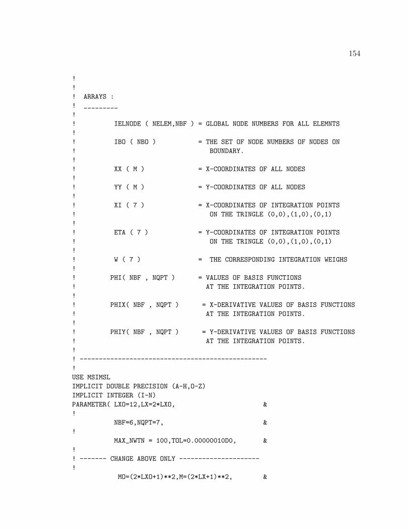
154
!!! ARRAYS :! _________!! IELNODE ( NELEM,NBF ) = GLOBAL NODE NUMBERS FOR ALL ELEMNTS!! IBO ( NBO ) = THE SET OF NODE NUMBERS OF NODES ON! BOUNDARY.!! XX ( M ) = X-COORDINATES OF ALL NODES!! YY ( M ) = Y-COORDINATES OF ALL NODES!! XI ( 7 ) = X-COORDINATES OF INTEGRATION POINTS! ON THE TRINGLE (0,0),(1,0),(0,1)!! ETA ( 7 ) = Y-COORDINATES OF INTEGRATION POINTS! ON THE TRINGLE (0,0),(1,0),(0,1)!! W ( 7 ) = THE CORRESPONDING INTEGRATION WEIGHS!! PHI( NBF , NQPT ) = VALUES OF BASIS FUNCTIONS! AT THE INTEGRATION POINTS.!! PHIX( NBF , NQPT ) = X-DERIVATIVE VALUES OF BASIS FUNCTIONS! AT THE INTEGRATION POINTS.!! PHIY( NBF , NQPT ) = Y-DERIVATIVE VALUES OF BASIS FUNCTIONS! AT THE INTEGRATION POINTS.!! -------------------------------------------------!USE MSIMSLIMPLICIT DOUBLE PRECISION (A-H,O-Z)IMPLICIT INTEGER (I-N)PARAMETER( LXO=12,LX=2*LXO, &!
NBF=6,NQPT=7, &!
MAX_NWTN = 100,TOL=0.00000010D0, &!! ------- CHANGE ABOVE ONLY ---------------------!
MO=(2*LXO+1)**2,M=(2*LX+1)**2, &

155
!NNZ=46*LX**2+16*LX+1,NBO=8*LX, &
!NELEM=2*LX*LX,NELEMO=2*LXO*LXO, &
!NBOO=8*LXO,NPT=2*LX+1, &
!NPTO=2*LXO+1,NIN=M-NBO,NINO=MO-NBOO &
!)
!DIMENSION IA(NNZ),JA(NNZ),IELNODE(NELEM,NBF), &
A(NNZ),XX(M),YY(M),SOLO(MO),EA(NBF,NBF), &B(NBF,NBF,NBF),IBO(NBO),IN(NIN), &XI(NQPT),ETA(NQPT),W(NQPT), &
PHI(NBF,NQPT),PHIX(NBF,NQPT), &PHIY(NBF,NQPT),SOLN(M),RHS(M), &ER(MAX_NWTN,2),VRE(5)
!DIMENSION INO(NINO),IBOO(NBOO),IELNODEO(NELEMO,NBF)!!!!VRE = (/1.0D0,100.0D0,100.0D0,1000.0D0,2000.0D0/)DO IRE=1,1RE = VRE(IRE)!!!!IF(RE == 10.0) THEN
OPEN(UNIT= 32,FILE="SOLO.DAT",STATUS="OLD")READ(32,*)SOLO
!ELSE IF( RE == 50.0) THEN! OPEN(UNIT= 32,FILE="SOLO50.DAT",STATUS="OLD")! READ(32,*)SOLO!ELSE IF( RE == 100.0) THEN! OPEN(UNIT= 32,FILE="SOLO100.DAT",STATUS="OLD")! READ(32,*)SOLO!ELSE IF( RE == 1000.0) THEN! OPEN(UNIT= 32,FILE="SOLO1000.DAT",STATUS="OLD")! READ(32,*)SOLO!ELSE! OPEN(UNIT= 32,FILE="SOLO2000.DAT",STATUS="OLD")! READ(32,*)SOLO

156
!END IF
!!CALL MAELNODE(IELNODE,IN,IBO,LX,NBO,NIN,M,NELEM,NBF,NPT)CALL MAELNODE(IELNODEO,INO,IBOO,LXO,NBOO,NINO,MO,NELEMO,NBF,NPTO)CALL COORD(XX,YY,LX,M)CALL MAEA(EA,NBF)CALL QUAD7(NQPT,XI,ETA,W)CALL PHIQ(PHI,PHIX,PHIY,NBF,NQPT,XI,ETA)CALL MAB(B,NBF)!!H=1.0D0/DBLE(LX)IA=0 ; JA = 0 ; A=0.0D0!TIME1=CPSEC()CALL FINE_LEVEL_SOLVE(SOLN, &
SOLO,IELNODE,NELEMO, &LX,LXO,RE,TOL,M,MO,IN,IBO,NIN, &NBO,NBF,NELEM,XX,YY,PHI,PHIX, &PHIY,XI,ETA,W,NQPT,EA,NNZ,B, &IELNODEO,KK)
TIME2=CPSEC()XCPU=TIME2-TIME1CALL PRINTOUT1(SOLN,ER,KK,XCPU, &
LX,RE,TOL,MAX,M,NIN,NQPT, &NBO,NBF,NELEM,NNZ)
!!PRINT*,’ I FINISH SUCESSFULLAY’!END DO!END PROGRAM FINE_STEP_TEST
SUBROUTINE FINE_LEVEL_SOLVE(SOLN, &SOLO,IELNODE,NELEMO, &
LX,LXO,RE,TOL,M,MO,IN,IBO,NIN, &NBO,NBF,NELEM,XX,YY,PHI,PHIX, &PHIY,XI,ETA,W,NQPT,EA,NNZ,B, &IELNODEO,KK)
IMPLICIT DOUBLE PRECISION (A-H,O-Z)IMPLICIT INTEGER (I-N)
157
DIMENSION SOLN(M),IELNODE(NELEM,NBF),SOLO(MO),&IBO(NBO),IN(NIN),XX(M), &
YY(M),PHI(NBF,NQPT),PHIX(NBF,NQPT), &PHIY(NBF,NQPT),XI(NQPT),ETA(NQPT), &W(NQPT),EA(NBF,NBF), &B(NBF,NBF,NBF),IELNODEO(NELEMO,NBF)
INTENT(OUT) :: SOLNINTENT(IN) :: IELNODE,IN,LX,RE,TOL,M, &
IBO,NIN,NBO,NBF,NELEM,XX,YY, &PHI,PHIX,PHIY,XI,ETA,W,NQPT, &EA,B,SOLO,IELNODEO
! LOCALDIMENSION A(NNZ),IA(NNZ),JA(NNZ),RHS(M)!!!CALL STIFF(A,IA,JA,NNZ,LX,NBF,M,RE,IELNODE,XX,YY,&
LXO,MO,IELNODEO,SOLO,EA,B,&NELEM,NELEMO)!!CALL RHS2L(RHS,LX,M,NIN,NBO,RE, &
NBF,IELNODE,IN,IBO,&XX,YY,PHI,PHIX,PHIY, &
XI,ETA,W,NQPT,NELEM )!!!CALL BOUNDARY_A(A,IA,JA,IBO,NNZ,NBO)CALL BOUNDARY_RHS(RHS,IBO,M,NBO)!!IF(RE == 10.0) THENOPEN(UNIT= 55,FILE="A10.DAT",STATUS="NEW")OPEN(UNIT= 56,FILE="RHS10.DAT",STATUS="NEW")
ELSE IF( RE == 50.0) THENOPEN(UNIT= 55,FILE="TA50L32.DAT",STATUS="NEW")OPEN(UNIT= 56,FILE="TRHS50L32.DAT",STATUS="NEW")
ELSE IF( RE == 100.0) THENOPEN(UNIT= 55,FILE="TA100L32.DAT",STATUS="NEW")OPEN(UNIT= 56,FILE="TRHS100L32.DAT",STATUS="NEW")
ELSE IF( RE == 1000.0) THENOPEN(UNIT= 55,FILE="A1000.DAT",STATUS="NEW")OPEN(UNIT= 56,FILE="RHS1000.DAT",STATUS="NEW")
ELSE
158
OPEN(UNIT= 55,FILE="A2000.DAT",STATUS="NEW")OPEN(UNIT= 56,FILE="RHS2000.DAT",STATUS="NEW")
END IFDO I=1,NNZWRITE(55,*) A(I),IA(I),JA(I)
END DODO I=1,MWRITE(56,*) RHS(I)
END DO!SOLN=0.0D0CALL BICGSTAB(SOLN,KK,RHS,TOL,A,IA,JA,NNZ,M,1)!!!END SUBROUTINE FINE_LEVEL_SOLVE!!!SUBROUTINE PRINTOUT1(SOL,ER,KK,CPU, &
LX,RE,TOL,MAX,M,NIN,NQPT, &NBO,NBF,NELEM,NNZ)
IMPLICIT DOUBLE PRECISION (A-H,O-Z)IMPLICIT INTEGER (I-N)DIMENSION SOL(M),ER(MAX,2),ITER(MAX)INTENT(IN) :: SOL,ER,KK,CPU,LX, &
RE,TOL,MAX,M,NQPT, &NIN,NBO,NBF,NELEM, &NNZ
IF(RE == 10.0) THENOPEN(UNIT= 31,FILE="STATN10.DAT",STATUS="NEW")OPEN(UNIT= 32,FILE="SOLN10.DAT",STATUS="NEW")
ELSE IF( RE == 50.0) THENOPEN(UNIT= 31,FILE="TS50L32.DAT",STATUS="NEW")OPEN(UNIT= 32,FILE="TSOL50L32.DAT",STATUS="NEW")
ELSE IF( RE == 100.0) THENOPEN(UNIT= 31,FILE="TS100L32.DAT",STATUS="NEW")OPEN(UNIT= 32,FILE="TSOL100L32.DAT",STATUS="NEW")
ELSE IF( RE == 1000.0) THENOPEN(UNIT= 31,FILE="STATN1000.DAT",STATUS="NEW")OPEN(UNIT= 32,FILE="SOLN1000.DAT",STATUS="NEW")
ELSEOPEN(UNIT= 31,FILE="STATN2000.DAT",STATUS="NEW")OPEN(UNIT= 32,FILE="SOLN2000.DAT",STATUS="NEW")
END IF

159
WRITE(31,*) ’ ------------------------------------’WRITE(31,*)WRITE(31,*) ’ LX = ’ , LXWRITE(31,*)WRITE(31,*) ’ RE = ’ , REWRITE(31,*)WRITE(31,*) ’ # ELEMENTS = ’ , NELEMWRITE(31,*)WRITE(31,*) ’ # OF NODES(M) = ’ , MWRITE(31,*)WRITE(31,*) ’ # OF BOUNDARY NODES(NBO) = ’,NBOWRITE(31,*)WRITE(31,*) ’ # OF INTIRIOR NODES(NIN) = ’,NINWRITE(31,*)WRITE(31,*) ’ # OF BASIS FUNCTIONS(NBF) = ’,NBFWRITE(31,*)WRITE(31,*) ’ # OF QUADRATURE POINTS(NQPT) = ’,NQPTWRITE(31,*)WRITE(31,*) ’ # OF MAXIMUM NEWTON ITERATIONS(MAX) = ’,MAXWRITE(31,*)WRITE(31,*) ’ # OF NONZERO ENTRY IN THE JACOBIAN(NNZ) = ’,NNZWRITE(31,*)WRITE(31,*) ’ THE TOLERANCE = ’,TOLWRITE(31,*)WRITE(31,*) ’ TOTAL CPU TIME IN SECONDS = ’, CPUWRITE(31,*)WRITE(31,*) ’ ------------------------------------’WRITE(31,*)WRITE(31,*) ’ #BCGS =’ ,KKWRITE(31,*)WRITE(31,*) ’ ------------------------------------’DO I=1,M
WRITE(31,*) SOL(I)WRITE(32,*) SOL(I)
END DO!END SUBROUTINE PRINTOUT1!!!SUBROUTINE COARSE_LEVEL_SOLVE( &
SOL,IELNODE,ER,ITER,CPU, &LX,RE,TOL,MAX,M,IN,IBO,NIN, &NBO,NBF,NELEM,XX,YY,PHI,PHIX, &PHIY,XI,ETA,W,NQPT,EA,NNZ,B &
160
)IMPLICIT DOUBLE PRECISION (A-H,O-Z)IMPLICIT INTEGER (I-N)DIMENSION SOL(M),IELNODE(NELEM,NBF), &
ITER(MAX),IBO(NBO),IN(NIN),XX(M), &YY(M),PHI(NBF,NQPT),PHIX(NBF,NQPT), &PHIY(NBF,NQPT),XI(NQPT),ETA(NQPT), &W(NQPT),EA(NBF,NBF),ER(MAX,2), &B(NBF,NBF,NBF)
INTENT(INOUT) :: SOLINTENT(OUT) :: ER,ITER,CPUINTENT(IN) :: IELNODE,IN,LX,RE,TOL,MAX,M, &
IBO,NIN,NBO,NBF,NELEM,XX,YY, &PHI,PHIX,PHIY,XI,ETA,W,NQPT, &EA,B
! LOCALDIMENSION UP(M),A(NNZ),IA(NNZ),JA(NNZ),RHS(M)UP = SOLER1= 1.0D0 ; XNORM =0.0D0 ; YNORM= 0.0D0DO I=1,MAX
CALL JACOBS(LX,M,NNZ,NELEM,NIN,NBO, &NBF,A,IA,JA,RE,SOL,IELNODE,&
IN,IBO,EA,B)!
CALL FORCE(RHS,LX,RE,SOL,IELNODE, &IN,IBO,XX,YY,PHI,PHIX, &
PHIY,XI,ETA,W,EA,NBF, &NELEM,M,NIN,NBO,NQPT,B)
!! IF( RATIO >= 1)THEN! PRINT*,’ NO IMPROVMENT FOR F(SOL)’! EXIT! END IF
CALL BOUNDARY_A(A,IA,JA,IBO,NNZ,NBO)CALL BOUNDARY_RHS(RHS,IBO,M,NBO)
!CALL NORM(XNORM,RHS,M)OLDER1=ER1ER1 = XNORM/DBLE(M)RATIO =ER1/OLDER1
CALL BICGSTAB(UP,KK,RHS,TOL,A,IA,JA,NNZ,M,I)ITER(I)=KKSOL = SOL - UPCALL NORM(YNORM,UP,M)
161
ER2 = YNORM/DBLE(M)ER(I,:)=(/ER1,ER2/)PRINT*,I,ER(I,:)IF(ER1<TOL .AND. ER2<TOL)THEN;EXIT;END IF
END DO!!END SUBROUTINE COARSE_LEVEL_SOLVE!!! STATUS = NOT OK! FIX HOW TO STORE A , IA , JASUBROUTINE STIFF(A,IA,JA,NNZ,LX,NBF,M,RE,IELNODE,XX,YY,&
LXO,MO,IELNODEO,SOLO,EA,B,&NELEM,NELEMO)IMPLICIT DOUBLE PRECISION (A-H,O-Z)IMPLICIT INTEGER (I-N)DIMENSION IA(NNZ),JA(NNZ),IELNODE(NELEM,NBF),&
IELNODEO(NELEMO,NBF)DIMENSION A(NNZ),XX(M),YY(M),SOLO(MO),EA(NBF,NBF)DIMENSION B(NBF,NBF,NBF)INTENT(IN) :: NNZ,LX,NBF,M,RE,IELNODE,XX,YY, &
LXO,MO,IELNODEO,SOLO,EA,B, &NELEM,NELEMO
INTENT(OUT) :: IA,JA,A! LOCALDIMENSION X(3),Y(3)!! --------------------------------------! COMPUTE SOME PARAMETERS OF PROBLEMS! DEPENDS ON LX! --------------------------------------CONT=0.0D0H = 1.0D0 / DBLE(LX)RATIO=DBLE(LX)/DBLE(LXO)!------------ASSIMBLE STIFF ------------INDEX =0A = 0.0D0; IA = 0 ; JA=0X=0.0D0;Y=0.0D0DO K=1,NELEMDO IX=1,3IP= IABS( IELNODE(K,IX))
X(IX) = XX(IP)Y(IX) = YY(IP)END DO

162
XM=( X(2)+X(3)+2.0D0*X(1) )/4.0D0YM=( Y(2)+Y(3)+2.0D0*Y(1) )/4.0D0DO IR =1,NBF
AIJ=0.0D0II = IELNODE(K,IR)
IROW = ABS(II)DO IS =1,NBFJJ=IELNODE(K,IS)D=DBLE(ISIGN(1,II)*ISIGN(1,JJ))JCOL = IABS(JJ)
CONT= (D/RE)*EA(IR,IS)/(H*H)!AF(IROW,JCOL) = AF(IROW,JCOL) + CONT
!AIJ = AIJ + (D/RE)*EA(IR,IS)/(H*H)CALL STORE(A,IA,JA,NNZ,IROW,JCOL,CONT,INDEX)SUM = 0.0D0
DO IK=1,NBFCALL FINDK(XM,YM,LXO,KO) ! KO=FINDK
K3=IELNODEO(KO,IK)KK= IABS(K3)D = DBLE(SIGN(1,II)*SIGN(1,JJ)*SIGN(1,K3))SUM=SUM + D*SOLO(KK)*B(IK,IR,IS)END DOSUM = SUM/(RATIO*H**2)!AF(IROW,JCOL) = AF(IROW,JCOL) + SUM!AIJ = AIJ + SUMCALL STORE(A,IA,JA,NNZ,IROW,JCOL,SUM,INDEX)END DO
END DOEND DO
END SUBROUTINE STIFF!!!SUBROUTINE BOUNDARY_A(A,IA,JA,IBO,NNZ,NBO)IMPLICIT DOUBLE PRECISION (A-H,O-Z)IMPLICIT INTEGER (I-N)DIMENSION A(NNZ),IA(NNZ),JA(NNZ),IBO(NBO)INTENT(INOUT) :: A,IA,JAINTENT(IN) :: NNZ,NBO,IBO!DO IZ = 1,NBO
DO IH=1,NNZIF(IA(IH)==IBO(IZ)) A(IH)=0.0D0

163
IF(JA(IH)==IBO(IZ)) A(IH)=0.0D0END DO
END DO
DO IZ = 1,NBODO IH=1,NNZIF(IA(IH)==IBO(IZ) .AND. JA(IH)==IBO(IZ)) THEN
A(IH)=1.0D0END IF
END DOEND DO!END SUBROUTINE BOUNDARY_A!!SUBROUTINE BOUNDARY_RHS(RHS,IBO,M,NBO)IMPLICIT DOUBLE PRECISION (A-H,O-Z)IMPLICIT INTEGER (I-N)DIMENSION RHS(M),IBO(NBO)INTENT(INOUT) :: RHSINTENT(IN) :: M,NBO,IBO!DO IR=1,NBORHS( IBO(IR) ) = 0.0D0
END DO!END SUBROUTINE BOUNDARY_RHS!!!-----------------------------------------SUBROUTINE BICGSTAB(X,K,B,TOL,C,IC,JC,NNZ,M,NWTN)IMPLICIT DOUBLE PRECISION (A-H,O-Z)IMPLICIT INTEGER (I-N)DIMENSION X(M),B(M),C(NNZ),IC(NNZ),JC(NNZ)INTENT(IN) :: B,TOL,C,IC,JC,NNZ,M,NWTNINTENT(INOUT) :: XINTENT(OUT) :: K! LOCALDIMENSION R(M),RH(M),P(M),V(M),S(M),T(M),UP(M)K=0R=0.0D0;RH=0.0D0;P=0.0D0;V=0.0D0;S=0.0D0T=0.0D0;UP=0.0D0;RA=0.0D0CALL ATX(R,C,X,IC,JC,NNZ,M) ! R=C*XR = B-RRH= R

164
DO I=1,M*MPRINT*,NWTN ,’-TH NEWTON’,I,’-TH BICG’CALL DOT(ROW,RH,R,M)IF(ROW == 0 ) EXITIF(I == 1) THENP = R
ELSEBETA = (ROW/ROWOLD)*(ALPHA/W)P = R + BETA*(P-W*V)
END IFP = PCALL ATX(V,C,P,IC,JC,NNZ,M) ! V=C*PCALL DOT(VAL,RH,V,M) ! VAL = RH’*VALPHA = ROW/VALS = R - ALPHA*VCALL NORM(XNORM,S,M)IF( XNORM <TOL) THENK=IX=X+ALPHA*PPRINT*,’I STOP BECAUSE NORM(S)<TOL’EXIT
END IFS = SCALL ATX(T,C,S,IC,JC,NNZ,M) !T = C*SCALL DOT(VAL2,T,S,M)CALL DOT(VAL3,T,T,M)W = VAL2/VAL3UP = ALPHA*P +W*SX = X + UPR = S - W*TIF(W == 0 ) THENPRINT*,’I CAN NOT CONTINUE ITERATION BECAUSE W = 0’EXIT
END IFCALL NORM(XUP,UP,M)CALL NORM(XR,R,M)IF( XUP < TOL .AND. XR < TOL ) THENK = IPRINT*,’I STOP BECAUSE NORM(R,UP)<TOL’EXIT
END IFROWOLD=ROW
END DOEND SUBROUTINE BICGSTAB!

165
!!-------------------------------SUBROUTINE DOT(VAL,X,Y,M)INTEGER I,MDOUBLE PRECISION X(M),Y(M),VALINTENT(IN) :: X,Y,MINTENT(OUT) :: VALVAL = 0.0D0DO I=1,MVAL = VAL + X(I)*Y(I)
END DOEND SUBROUTINE DOT!!SUBROUTINE NORM(VAL,X,M)INTEGER I,MDOUBLE PRECISION VAL,X(M)INTENT(IN) :: X,MINTENT(OUT) :: VALVAL=0.0D0DO I=1,MVAL = VAL + X(I)*X(I)
END DOVAL = DSQRT(VAL)END SUBROUTINE NORM!!!----------------------------------SUBROUTINE ATX(Y,A,X,IA,JA,NNZ,M)INTEGER I,J,K,M,NNZINTEGER IA(NNZ),JA(NNZ)DOUBLE PRECISION X(M),Y(M),A(NNZ),AIJINTENT(IN) :: A,X,IA,JA,NNZ,MINTENT(OUT) :: YY=0.0D0DO K=1,NNZI=IA(K)J=JA(K)AIJ=A(K)Y(I)= Y(I) + AIJ*X(J)
END DOEND SUBROUTINE ATX!!----------------------------------SUBROUTINE ATTX(Y,A,X,IA,JA,NNZ,M)

166
INTEGER I,J,K,M,NNZINTEGER IA(NNZ),JA(NNZ)DOUBLE PRECISION X(M),Y(M),A(NNZ),AJIINTENT(IN) :: A,X,IA,JA,NNZ,MINTENT(OUT) :: YY=0.0D0DO K=1,NNZJ=IA(K)I=JA(K)AJI=A(K)Y(I)= Y(I) + AJI*X(J)
END DOEND SUBROUTINE ATTX!!!! STATUS( STORE ) =OK!SUBROUTINE STORE(A,IA,JA,NNZ,IROW,JCOL,AIJ,INDEX)DOUBLE PRECISION A(NNZ),AIJINTEGER IA(NNZ),JA(NNZ),IROW,JCOL,IFLAGINTEGER INDEXINTENT(INOUT) :: A,IA,JA,INDEXINTENT(IN) :: IROW,JCOL,NNZ,AIJCALL CHK(NNZ,IA,JA,IROW,JCOL,IFLAG)IF( IFLAG == 0) THENINDEX = INDEX + 1A(INDEX) = AIJIA(INDEX) = IROWJA(INDEX) = JCOL
ELSEA(IFLAG) = A(IFLAG) + AIJ
END IFEND SUBROUTINE STORE!!! STATUS( CHK ) = OK!SUBROUTINE CHK(NNZ,IA,JA,IROW,JCOL,IFLAG)INTEGER NNZ,IA(NNZ),JA(NNZ),JCOL,IROWINTENT(IN) :: NNZ,IA,JA,IROW,JCOLINTENT(OUT) :: IFLAGINTEGER IFLAG,IIFLAG = 0DO I=1,NNZ
167
IF( IA(I) == IROW .AND. JA(I) == JCOL ) THENIFLAG = I
EXITEND IF
END DOEND SUBROUTINE CHK!! STATUS( FINDK ) = OK!SUBROUTINE FINDK(X,Y,LX,K)IMPLICIT DOUBLE PRECISION (A-H,O-Z)IMPLICIT INTEGER (I-N)INTENT(IN) :: X,Y,LXINTENT(OUT) :: KH = 1.0D0/DBLE(LX)XK = 0.0D0 ; YK = 0.0D0 ;I =LX;J=LX;DO IK= 1,LXXK=XK+HIF( XK > X ) THENI=IK
EXITEND IF
END DODO JK =1,LXYK=YK +HIF( YK > Y) THENJ=JK
EXITEND IF
END DOSW = Y + X - H*DBLE(J+I-1)K=2*( (J-1)*LX +I ) - 1IF( SW > 0 ) THENK=K+1
END IFEND SUBROUTINE FINDK!! STATUS( RHS2L ) = OK!SUBROUTINE RHS2L(RHS,LX,M,NIN,NBO,RE, &
NBF,IELNODE,IN,IBO,&XX,YY,PHI,PHIX,PHIY, &
XI,ETA,W,NQPT,NELEM )IMPLICIT DOUBLE PRECISION (A-H,O-Z)
168
IMPLICIT INTEGER (I-N)DIMENSION RHS(M),IELNODE(NELEM,NBF),IN(NIN), &
IBO(NBO),XX(M),YY(M),PHI(NBF,NQPT), &PHIX(NBF,NQPT),PHIY(NBF,NQPT), &XI(NQPT),ETA(NQPT),W(NQPT)
INTENT(IN) :: IELNODE,IN,IBO,XX,YY,PHI,PHIX,PHIY, &XI,ETA,W,LX,M,NIN,NBO,RE,NBF, &
NQPT,NELEMINTENT(OUT) :: RHS! LOCALDIMENSION X(3),Y(3)H=1.0D0/DBLE(LX)RHS = 0.0D0DO NK=1,NELEMDO II=1,3X(II) = XX( IABS(IELNODE(NK,II)) )
Y(II) = YY( IABS(IELNODE(NK,II)) )END DO
! --------------------------------------DO IR=1,6
II=IELNODE(NK,IR)I =IABS(II)D= DBLE(SIGN(1,II))
SUM1=0 ; SUM2= 0DO IZ=1,7S=(X(2)-X(1))*XI(IZ) + X(1)T=(Y(3)-Y(1))*ETA(IZ) + Y(1)CALL F1(S,T,RE,F1ST)CALL F2(S,T,RE,F2ST)SUM1=SUM1 + W(IZ)*PHIY(IR,IZ)*F1STSUM2=SUM2 + W(IZ)*PHIX(IR,IZ)*F2ST
END DOVALUE =-SUM1*( X(2)-X(1) ) + SUM2*( Y(3)-Y(1) )RHS(I) = RHS(I) + D*VALUEEND DO
END DO!!END SUBROUTINE RHS2L!! STATUS = OK!SUBROUTINE F1(X,Y,RE,F1XY)IMPLICIT DOUBLE PRECISION (A-H,O-Z)IMPLICIT INTEGER (I-N)
169
INTENT(IN) X,Y,REINTENT(OUT) F1XY!D1=12.0D0*(-1.0D0 + X)**2*X**2*(-1.0D0 + Y)D2=12.0D0*(-1.0D0 + X)**2*X**2*YD3=4.0D0*(-1.0D0 + X)**2*(-1.0D0 + Y)**2*YD4=16.0D0*(-1.0D0 + X)*X*(-1.0D0 + Y)**2*YD5=4.0D0*X**2*(-1.0D0 + Y)**2*YD6=4.0D0*(-1.0D0 + X)**2*(-1.0D0 + Y)*Y**2D7=16.0D0*(-1.0D0 + X)*X*(-1.0D0 + Y)*Y**2D8=4.0D0*X**2*(-1.0D0 + Y)*Y**2D = -(D1+D2+D3+D4+D5+D6+D7+D8)/RE!---------------------------------------E1=3.0D0+ 4.0D0*X*Y**2 - 20.0D0*X**2*Y**2E2=36.0D0*X**3*Y**2 - 28.0D0*X**4*Y**2E3=8.0D0*X**5*Y**2 - 16.0D0*X*Y**3E4=80.0D0*X**2*Y**3 - 144.0D0*X**3*Y**3E5=112.0D0*X**4*Y**3 - 32.0D0*X**5*Y**3E6=28.0D0*X*Y**4 - 140.0D0*X**2*Y**4E7=252.0D0*X**3*Y**4 - 196.0D0*X**4*Y**4E8=56.0D0*X**5*Y**4 - 24.0D0*X*Y**5E9=120.0D0*X**2*Y**5 - 216.0D0*X**3*Y**5E10=168.0D0*X**4*Y**5 - 48.0D0*X**5*Y**5E11=8.0D0*X*Y**6 - 40.0D0*X**2*Y**6E12=72.0D0*X**3*Y**6 - 56.0D0*X**4*Y**6E13=16.0D0*X**5*Y**6E = X**2*(E1+E2+E3+E4+E5+E6+E7+E8+E9+E10+E11+E12+E13)F1XY = D + E!END SUBROUTINE F1!! STATUS = OK!SUBROUTINE F2(X,Y,RE,F2XY)IMPLICIT DOUBLE PRECISION (A-H,O-Z)IMPLICIT INTEGER (I-N)INTENT(IN) :: X,Y,REINTENT(OUT) :: F2XYD1=4.0D0*(-1.0D0 + X)**2*X*(-1.0D0 + Y)**2D2=4.0D0*(-1.0D0 + X)*X**2*(-1.0D0 + Y)**2D3=16.0D0*(-1.0D0 + X)**2*X*(-1.0D0 + Y)*YD4=16.0D0*(-1.0D0 + X)*X**2*(-1.0D0 + Y)*YD5=4.0D0*(-1.0D0 + X)**2*X*Y**2D6=4.0D0*(-1.0D0 + X)*X**2*Y**2D7=12.0D0*(-1.0D0 + X)*(-1.0D0 + Y)**2*Y**2

170
D8=12.0D0*X*(-1.0D0 + Y)**2*Y**2D = -(-D1-D2-D3-D4-D5-D6-D7-D8)/RE!---------------------------------------E1= 3.0D0+4.0D0*X**2*Y - 16.0D0*X**3*YE2=28.0D0*X**4*Y - 24.0D0*X**5*Y + 8.0D0*X**6*YE3=-20.0D0*X**2*Y**2 + 80.0D0*X**3*Y**2E4=-140.0D0*X**4*Y**2 + 120.0D0*X**5*Y**2E5=-40.0D0*X**6*Y**2 + 36.0D0*X**2*Y**3E6=-144.0D0*X**3*Y**3 + 252.0D0*X**4*Y**3E7=-216.0D0*X**5*Y**3 + 72.0D0*X**6*Y**3E8=-28.0D0*X**2*Y**4 + 112.0D0*X**3*Y**4E9=-196.0D0*X**4*Y**4 + 168.0D0*X**5*Y**4E10=-56.0D0*X**6*Y**4 + 8.0D0*X**2*Y**5E11=-32.0D0*X**3*Y**5 + 56.0D0*X**4*Y**5E12=-48.0D0*X**5*Y**5 + 16.0D0*X**6*Y**5E = Y**2*(E1+E2+E3+E4+E5+E6+E7+E8+E9+E10+E11+E12)F2XY = D + EEND SUBROUTINE F2!! STATUS = OK!SUBROUTINE MAELNODE(IELNODE,IN,IBO,LX,NBO,NIN,M,NELEM,NBF,NPT)IMPLICIT DOUBLE PRECISION (A-H,O-Z)IMPLICIT INTEGER (I-N)INTENT(IN) :: LX,NBO,NIN,NBF,NPTINTENT(OUT) :: IELNODE,IN, IBODIMENSION IELNODE(NELEM,NBF),IN(NIN),IBO(NBO)IELNODE=0;IN=0;IBO=0IELEMN=0! ODD TRAIANGLESDO I=1,LXDO J=1,LX
IELEMN=2*J-1 +2*LX*(I-1)K = 2*J-1 + 2*NPT*(I-1)IELNODE(IELEMN,1)= KIELNODE(IELEMN,2)= K+2IELNODE(IELEMN,3)= K+2*NPTIELNODE(IELEMN,4)= K+1IELNODE(IELEMN,5)= K+1+NPTIELNODE(IELEMN,6)= K+NPTEND DO
END DO!------------------! EVEN TRAIANGLES!------------------
171
DO I=1,LXDO J=1,LX
IELEMN=2*J +2*LX*(I-1)K = 2*NPT*I +2*J+1IELNODE(IELEMN,1)= KIELNODE(IELEMN,2)= K-2IELNODE(IELEMN,3)= K-2*NPTIELNODE(IELEMN,4)= K-1IELNODE(IELEMN,5)= K-1-NPTIELNODE(IELEMN,6)= K-NPTEND DO
END DODO I=1,LX*LXIELNODE(2*I,4) = - IELNODE(2*I,4)IELNODE(2*I,5) = - IELNODE(2*I,5)IELNODE(2*I,6) = - IELNODE(2*I,6)
END DO! CHANGE NORMAL POINTS ON EVEN TRIANGLE! ON X=1DO I=1,LXIELEMN= 2*LX*IIELNODE(IELEMN,6) = - IELNODE(IELEMN,6)
END DO! CHANGE NORMAL POINTS ON Y=1IELEMN = 2*LX*LXDO I=1,LX
IELEMN= IELEMN - 2*(I-1)IELNODE(IELEMN,4) = - IELNODE(IELEMN,4)
END DO!DO I=1,NPTIBO(I) = IIBO(I+NPT) = M-I+1
END DODO I=2,NPT-1IBO(I+2*NPT-1) = I*NPTIBO(3*NPT-3+I) = (I-1)*NPT + 1
END DO!INDEX=1DO I=2,NPT-1KK=(I-1)*NPT +1DO J=1,NPT-2IN(INDEX) = KK +J
INDEX = INDEX + 1

172
END DOEND DOEND SUBROUTINE MAELNODE!!!! STATUS = OK!SUBROUTINE COORD(X,Y,LX,M)DOUBLE PRECISION, INTENT(OUT) :: X(M),Y(M)INTEGER, INTENT(IN) :: LX,MDOUBLE PRECISION H,HHINTEGER NPT,I,J,NH=1.0D0/DBLE(LX)HH=H/2.0D0NPT = 2*LX+1X=0.0D0Y=0.0D0DO I=1,NPT
DO J=1,NPTN=J + (I-1)*NPTY(N) = (I-1)*HHX(N) = (J-1)*HH
END DOEND DOEND SUBROUTINE COORD!!!! STATUS = OK!SUBROUTINE QUAD7(NQPT,XI,ETA,W)DOUBLE PRECISION, INTENT(OUT) :: XI(NQPT),ETA(NQPT),W(NQPT)DOUBLE PRECISION THDINTEGER, INTENT(IN) :: NQPT! FOR GAUSS QUADRATUAL WITH 7-POINTS! EXACT WITH 4 DEGREES POLYTHD = 1.0D0/3.0D0XI =(/0.0D0,.50D0,1.0D0,.50D0,0.0D0,0.0D0,THD/)ETA=(/0.0D0,0.0D0,0.0D0,.50D0,1.0D0,.50D0,THD/)W =(/1.0D0/40.0D0,1.0D0/15.0D0,1.0D0/40.0D0, &
1.0D0/15.0D0,1.0D0/40.0D0,1.0D0/15.0D0,9.0D0/40.0D0/)! FOR GAUSS-LEGENDER INTEGRALS WITH 7-POINTS! EXACT WITH 13 DEGREES POLYEND SUBROUTINE QUAD7

173
!! STATUS = OK!SUBROUTINE PHIQ(PHI,PHIX,PHIY,NBF,NQPT,XI,ETA)IMPLICIT DOUBLE PRECISION (A-H,O-Z)IMPLICIT INTEGER (I-N)DIMENSION PHI(NBF,NQPT),PHIX(NBF,NQPT),PHIY(NBF,NQPT)DIMENSION XI(NQPT),ETA(NQPT)INTENT(OUT) :: PHI,PHIX,PHIYINTENT(IN) :: NBF,NQPT,XI,ETAPHI=0.0D0PHIX=0.0D0PHIY=0.0D0DO I=1,NQPTX=XI(I)Y=ETA(I)PHI(1,I) = 1.0D0-X-Y+2.0D0*X*YPHI(2,I) = X/2.0D0 + X**2/2.0D0 + Y/2.0D0 -X*Y-Y**2/2.0D0PHI(3,I) = X/2.0D0-X**2/2.0D0+Y/2.0D0-X*Y+Y**2/2.0D0PHI(4,I) = -Y+Y**2PHI(5,I) = (-X+X**2-Y+2.0D0*X*Y+Y**2)/DSQRT(2.0D0)PHI(6,I) = -X+X**2PHIX(1,I) = -1.0D0+2.0D0*YPHIX(2,I) = 1.0D0/2.0D0 + X-YPHIX(3,I) = 1.0D0/2.0D0-X-YPHIX(4,I) = 0.0D0PHIX(5,I) = DSQRT(2.0D0)*(-0.50D0+X+Y)PHIX(6,I) = -1.0D0+2.0D0*XPHIY(1,I) = -1.0D0+2.0D0*XPHIY(2,I) = 0.50D0 -X-YPHIY(3,I) = 0.50D0-X+YPHIY(4,I) = -1.0D0+2.0D0*YPHIY(5,I) = DSQRT(2.0D0)*(-0.50D0+X+Y)PHIY(6,I) = 0.0D0
END DOEND SUBROUTINE PHIQ!! STATUS = OK!SUBROUTINE MAEA(EA,NBF)DOUBLE PRECISION, INTENT(OUT) :: EA(NBF,NBF)INTEGER, INTENT(IN) :: NBFEA= RESHAPE( &
(/4.0D0,-2.0D0,-2.0D0,0.0D0,2.828430D0,0.0D0, &-2.0D0,2.0D0,0.0D0,-1.0D0,-1.414210D0,1.0D0, &
174
-2.0D0,0.0D0,2.0D0,1.0D0,-1.414210D0,-1.0D0, &0.0D0,-1.0D0,1.0D0,2.0D0,1.414210D0,0.0D0 , &2.828430D0,-1.414210D0,-1.414210D0,1.414210D0, &4.0D0,1.414210D0,0.0D0,1.0D0,-1.0D0,0.0D0, &1.414210D0,2.0D0/),&
(/NBF,NBF/) )END SUBROUTINE MAEA!!! STATUS( JACOBS ) = OK!SUBROUTINE JACOBS(LX,M,NNZ,NELEM,NIN,NBO, &
NBF,A,IA,JA,RE,SOL,IELNODE,&IN,IBO,EA,B)
IMPLICIT DOUBLE PRECISION (A-H,O-Z)IMPLICIT INTEGER (I-N)INTENT(IN) :: LX,M,NNZ,NELEM,NIN, &
NBO,NBF,RE,SOL, &IELNODE,IN,IBO,EA,B
INTENT(OUT) :: A,IA,JADIMENSION A(NNZ),IA(NNZ),JA(NNZ), &
IELNODE(NELEM,NBF), &IN(NIN),IBO(NBO), &
SOL(M),EA(NBF,NBF), &B(NBF,NBF,NBF)
!H = 1.0D0 / DBLE(LX)!------------ASSIMBLE STIFF ----------IA= 0 ; JA = 0 ; A = 0.0D0INDEX = 0DO K=1,NELEMDO IR =1,NBF
II = IELNODE(K,IR)I = ABS(II)DO IS =1,NBFJJ=IELNODE(K,IS)D=DBLE(SIGN(1,II)*SIGN(1,JJ))J = ABS(JJ)!AF(I,J) = AF(I,J) + (D/RE)*EA(IR,IS)/H**2
CONT = (D/RE)*EA(IR,IS)/H**2CALL STORE(A,IA,JA,NNZ,I,J,CONT,INDEX)SUM = 0.0D0DO IK=1,NBFK3=IELNODE(K,IK)
KK= ABS(K3)
175
D = DBLE(SIGN(1,II)*SIGN(1,JJ)*SIGN(1,K3))BRACK = B(IR,IS,IK) + B(IR,IK,IS)SUM=SUM + D*SOL(KK)*BRACK/H**2IF(K==2 .AND. IR==4 .AND. IS==2 .AND. IK==4)THENEND IF
END DO!AF(I,J) = AF(I,J) + SUMCALL STORE(A,IA,JA,NNZ,I,J,SUM,INDEX)END DO
END DOEND DO!END SUBROUTINE JACOBS!! STATUS( FORCE ) = OK!SUBROUTINE FORCE(RHS,LX,RE,SOL,IELNODE, &
IN,IBO,XX,YY,PHI,PHIX, &PHIY,XI,ETA,W,EA,NBF, &
NELEM,M,NIN,NBO,NQPT,B)IMPLICIT DOUBLE PRECISION (A-H,O-Z)IMPLICIT INTEGER (I-N)DIMENSION RHS(M),SOL(M),IN(NIN), &
IELNODE(NELEM,NBF),IBO(NBO), &XX(M),YY(M),PHI(NBF,NQPT), &PHIX(NBF,NQPT),PHIY(NBF,NQPT),&XI(NQPT),ETA(NQPT),W(NQPT), &EA(NBF,NBF),B(NBF,NBF,NBF)
! LOCADIMENSION X(3),Y(3)INTENT(IN) :: LX,RE,SOL,IELNODE,IN, &
IBO,XX,YY,PHI,PHIX, &PHIY,XI,ETA,W,EA,B, &NBF,NELEM,M,NIN,NBO, &NQPT
H=1.0D0/DBLE(LX)RHS = 0.0D0DO NK=1,NELEMDO II=1,3X(II) = XX( ABS(IELNODE(NK,II)) )
Y(II) = YY( ABS(IELNODE(NK,II)) )END DO
! --------------------------------------DO IR=1,6
II=IELNODE(NK,IR)
176
I=ABS(II)D=DBLE(SIGN(1,II))
SUM1=0.0D0 ; SUM2= 0.0D0DO IZ=1,7S=(X(2)-X(1))*XI(IZ) + X(1)T=(Y(3)-Y(1))*ETA(IZ) + Y(1)CALL F1(S,T,RE,F1ST)CALL F2(S,T,RE,F2ST)SUM1=SUM1 + W(IZ)*PHIY(IR,IZ)*F1STSUM2=SUM2 + W(IZ)*PHIX(IR,IZ)*F2ST
END DOVALUE =-SUM1*( X(2)-X(1) ) + SUM2*( Y(3)-Y(1) )RHS(I) = RHS(I) + D*VALUE! ----------------------------SUM=0.0D0DO IS=1,NBFJJ=IELNODE(NK,IS)J=ABS(JJ)D=DBLE(SIGN(1,II)*SIGN(1,JJ))SUM = SUM + (D/RE)*EA(IR,IS)*SOL(J)
END DORHS(I) = RHS(I) + SUM/H**2! -----------------------------
SUM=0.0D0DO IS=1,NBFJJ=IELNODE(NK,IS)J=ABS(JJ)DO IK=1,NBF
KK= IELNODE(NK,IK)K= ABS(KK)D=DBLE(SIGN(1,II)*SIGN(1,JJ)*SIGN(1,KK))SUM=SUM+D*B(IR,IK,IS)*SOL(K)*SOL(J)
END DOEND DORHS(I) = RHS(I) + SUM/H**2! ---------------------------END DO
END DO!END SUBROUTINE FORCE!!!SUBROUTINE MAB(B,NBF)DOUBLE PRECISION, INTENT(OUT) :: B(NBF,NBF,NBF)
177
INTEGER, INTENT(IN) :: NBFB= RESHAPE( (/ &0.000000000000000E+000, &0.000000000000000E+000, &0.000000000000000E+000, &0.000000000000000E+000, &4.714045200000000E-001, &0.000000000000000E+000, &0.000000000000000E+000, &1.666666700000000E-001, &-1.666666700000000E-001, &1.666666700000000E-001, &0.000000000000000E+000, &1.666666700000000E-001, &0.000000000000000E+000, &-1.666666700000000E-001, &1.666666700000000E-001, &-1.666666700000000E-001, &-4.714045200000000E-001, &-1.666666700000000E-001, &0.000000000000000E+000, &-3.333333300000000E-001, &3.333333300000000E-001, &0.000000000000000E+000, &-4.714045200000000E-001, &-3.333333300000000E-001, &0.000000000000000E+000, &-2.357022600000000E-001, &2.357022600000000E-001, &2.357022600000000E-001, &0.000000000000000E+000, &-2.357022600000000E-001, &0.000000000000000E+000, &0.000000000000000E+000, &0.000000000000000E+000, &3.333333300000000E-001, &0.000000000000000E+000, &0.000000000000000E+000, &0.000000000000000E+000, &-3.333333300000000E-001, &3.333333300000000E-001, &0.000000000000000E+000, &
-1.178511300000000, &-3.333333300000000E-001, &1.666666700000000E-001, &

178
-2.500000000000000E-001, &8.333333300000000E-002, &-1.666666700000000E-001, &5.892556500000000E-001, &0.000000000000000E+000, &-1.666666700000000E-001, &5.833333300000000E-001, &-4.166666700000000E-001, &1.666666700000000E-001, &5.892556500000000E-001, &3.333333300000000E-001, &0.000000000000000E+000, &4.166666700000000E-001, &-4.166666700000000E-001, &0.000000000000000E+000, &5.892556500000000E-001, &3.333333300000000E-001, &2.357022600000000E-001, &-2.357022600000000E-001, &0.000000000000000E+000, &-2.357022600000000E-001, &0.000000000000000E+000, &0.000000000000000E+000, &3.333333300000000E-001, &-4.166666700000000E-001, &8.333333300000000E-002, &-3.333333300000000E-001, &5.892556500000000E-001, &0.000000000000000E+000, &0.000000000000000E+000, &3.333333300000000E-001, &-3.333333300000000E-001, &0.000000000000000E+000, &7.071067800000001E-001, &3.333333300000000E-001, &-1.666666700000000E-001, &8.333333300000000E-002, &8.333333300000000E-002, &0.000000000000000E+000, &-5.892556500000000E-001, &-1.666666700000000E-001, &1.666666700000000E-001, &-4.166666700000000E-001, &2.500000000000000E-001, &0.000000000000000E+000, &
179
-1.178511300000000E-001, &-1.666666700000000E-001, &0.000000000000000E+000, &-8.333333300000000E-002, &8.333333300000000E-002, &0.000000000000000E+000, &-1.178511300000000E-001, &0.000000000000000E+000, &-2.357022600000000E-001, &4.714045200000000E-001, &-2.357022600000000E-001, &0.000000000000000E+000, &0.000000000000000E+000, &2.357022600000000E-001, &-3.333333300000000E-001, &4.166666700000000E-001, &-8.333333300000000E-002, &0.000000000000000E+000, &-5.892556500000000E-001, &0.000000000000000E+000, &0.000000000000000E+000, &0.000000000000000E+000, &0.000000000000000E+000, &3.333333300000000E-001, &0.000000000000000E+000, &0.000000000000000E+000, &1.666666700000000E-001, &-1.666666700000000E-001, &0.000000000000000E+000, &-1.666666700000000E-001, &0.000000000000000E+000, &0.000000000000000E+000, &-1.666666700000000E-001, &1.666666700000000E-001, &0.000000000000000E+000, &-1.666666700000000E-001, &0.000000000000000E+000, &0.000000000000000E+000, &-3.333333300000000E-001, &3.333333300000000E-001, &0.000000000000000E+000, &0.000000000000000E+000, &0.000000000000000E+000, &0.000000000000000E+000, &-2.357022600000000E-001, &

180
2.357022600000000E-001, &0.000000000000000E+000, &2.357022600000000E-001, &0.000000000000000E+000, &0.000000000000000E+000, &0.000000000000000E+000, &0.000000000000000E+000, &0.000000000000000E+000, &0.000000000000000E+000, &0.000000000000000E+000, &0.000000000000000E+000, &4.714045200000000E-001, &
-1.178511300000000, &7.071067800000001E-001, &0.000000000000000E+000, &0.000000000000000E+000, &-4.714045200000000E-001, &0.000000000000000E+000, &5.892556500000000E-001, &-5.892556500000000E-001, &0.000000000000000E+000, &8.333333300000000E-001, &4.714045200000000E-001, &-4.714045200000000E-001, &5.892556500000000E-001, &-1.178511300000000E-001, &0.000000000000000E+000, &-8.333333300000000E-001, &0.000000000000000E+000, &0.000000000000000E+000, &-5.892556500000000E-001, &5.892556500000000E-001, &0.000000000000000E+000, &-8.333333300000000E-001, &-4.714045200000000E-001, &6.666666700000000E-001, &
-1.666666700000000, &1.000000000000000, &
0.000000000000000E+000, &0.000000000000000E+000, &-6.666666700000000E-001, &4.714045200000000E-001, &-5.892556500000000E-001, &1.178511300000000E-001, &0.000000000000000E+000, &

181
8.333333300000000E-001, &0.000000000000000E+000, &0.000000000000000E+000, &-3.333333300000000E-001, &3.333333300000000E-001, &0.000000000000000E+000, &-4.714045200000000E-001, &-3.333333300000000E-001, &1.666666700000000E-001, &0.000000000000000E+000, &-1.666666700000000E-001, &0.000000000000000E+000, &4.714045200000000E-001, &1.666666700000000E-001, &-1.666666700000000E-001, &3.333333300000000E-001, &-1.666666700000000E-001, &0.000000000000000E+000, &0.000000000000000E+000, &1.666666700000000E-001, &0.000000000000000E+000, &0.000000000000000E+000, &0.000000000000000E+000, &0.000000000000000E+000, &0.000000000000000E+000, &0.000000000000000E+000, &2.357022600000000E-001, &-4.714045200000000E-001, &2.357022600000000E-001, &0.000000000000000E+000, &0.000000000000000E+000, &-2.357022600000000E-001, &3.333333300000000E-001, &-3.333333300000000E-001, &0.000000000000000E+000, &0.000000000000000E+000, &4.714045200000000E-001, &0.000000000000000E+000 &/),&(/NBF,NBF,NBF/), &ORDER = (/3,2,1/) &)
END SUBROUTINE MAB
Appendix B
FORTRAN 77 Program UsingBogner-Fox-Schmit Element
182

183
C -------------------------------------------------C THIS PROGRAM IS FOR SOLVING THE NAVIER-STOKESC EQUATIONS USING THE TWO LEVEL FINITE ELEMENTC METHOD ON THE STREAM FUNCTION FORMULATIONC FOR A FULL DESCRIPTION OF THE METHOD SEEC F. FAIRAG, TWO-LEVEL FINITE ELEMENT METHODC FOR THE STREAM FUNCTION FORMULATION OF THEC NAVIER-STOKES EQUATIONS, TO BE APPEAR INC INTERNATIONAL JOURNAL COMPUTERS AND MATHEMATICSC WITH APPLICATIONS.CC THERE ARE TWO VERSION OF THIS CODE. THIS ONEC USES THE BOGNER-FOX-SCHMIDT ELEMENT. THE OTHERC USES THE MORLEY ELEMENTS. FOR A DESCRIPTION ABOUTC THESE ELEMENTS SEE THE ABOVE REFERENCE OR PH. G.C CIARLET, THE FINITE ELEMENT METHOD FOR ELLIPTICC PROBLEMS,1978.CC CONSIDER THE FOLLOWING EQUATION :C ------------------------- IN LATEX FORM ------------C \BEGINEQUATIONC \BEGINSPLITC RE^-1 \BIGTRIANGLEUP^2 \PSI-C \PSI_Y \BIGTRIANGLEUP \PSI_XC +\PSI_X \BIGTRIANGLEUP \PSI_Y& =C \VEC\MBOXCURL\VECF, \MBOX IN \OMEGA, \\C \PSI& = 0, \MBOX ON \PARTIAL \OMEGA, \\C \FRAC\PARTIAL\PSI\PARTIAL\HATN& = 0,C \MBOX ON \PARTIAL \OMEGA.C \ENDSPLITC \ENDEQUATIONC WHERE $ \HATN $ REPRESENTS THE OUTWARD UNITC NORMAL TO $ \OMEGA $.C -------------------- IN TEXT FORM --------------------C 1 2C ___ ( LAP ) PSI(X,Y) + R(PSI_X,PSI_Y) = F(X,Y) IN OMEGAC REC PSI(X,Y) = 0 ON BOUNDARYCC PARTIAL(PSI)/PARTIAL(N) = 0 ON BOUNDARYCC WHERECC LAP (F) = LAPLACIAN OF F = F_XX + F_YYC

184
C R(F,G) = F * LAP(G) - G * LAP(F)CCC BOGNER-FOX-SCHMEDIT RECTANGLE :C _______________________________CC FOR THE BFS RECTANGULAR ELEMENT WE HAVE THAT THE FUNCTIONSC ARE BICUBIC POLYNOMIALS WITHIN EACH ELEMENT. THE DEGREES OFC FREEDOM ARE CHOSEN TO BE THE FUNCTION VALUE , THE FIRSTC DERIVATIVES, AND MIXED SECOND DERIVATIVE AT THE VERTICES.C SO THE DIMENSION IS 16.CC SYMBOLS :C _________CCC LX = # OF ELEMENTS ALONG X-AXISCC LXO = # OF ELEMENTS ALONG X-AXISC IN THE COARSE MESHCC RE = REYNOLDS NUMBERCC NELEM = # OF ELEMENTS = LX*LXCC NPTS = # OF POINTS = (LX+1)*(LX+1)CC NBO = # OF BOUNDARY POINTS ON THEC ALL BOUNDARY EXCEPT THE TOPC WHICH RELATES TO Y-DERIVATIV= 15*LX - 1CC NBOY = # OF BOUNDARY POINTS ON THE TOPC WHICH RELATES TO Y-DERIVATIVE= LX+1CC NBF = # OF BASIS FUNCTIONS = 16CC M = # OF DEGREES OF FREEDOM = 4*NPTSCC NNZ = # OF NONZERO ENTRIES IN THEC JACOBIAN MATRIX = 36*MCC MAX = MAXIMUM NUMBER OF NEWTONC ITERATIONS TO SOLVE THE NONLINEARC SYSTEM RESULTING FROM COARSE MESHC
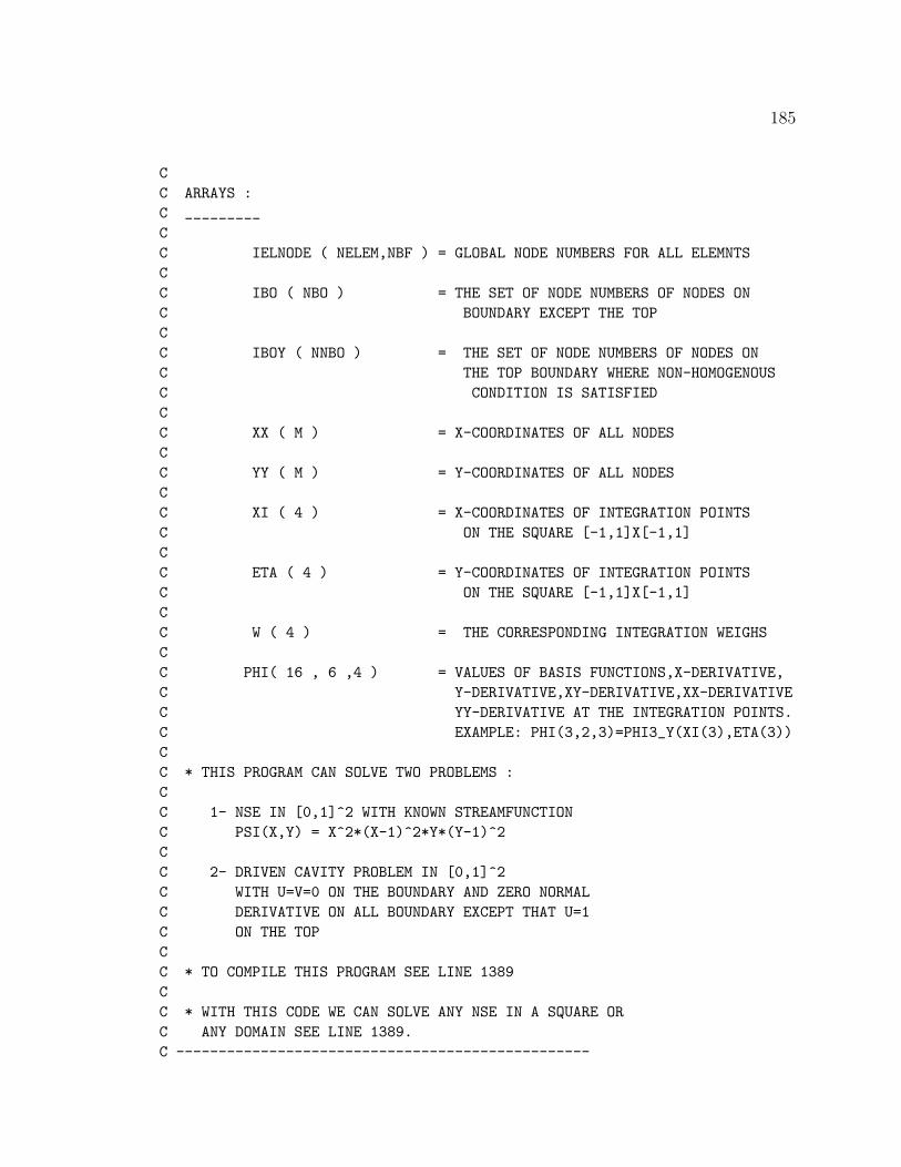
185
CC ARRAYS :C _________CC IELNODE ( NELEM,NBF ) = GLOBAL NODE NUMBERS FOR ALL ELEMNTSCC IBO ( NBO ) = THE SET OF NODE NUMBERS OF NODES ONC BOUNDARY EXCEPT THE TOPCC IBOY ( NNBO ) = THE SET OF NODE NUMBERS OF NODES ONC THE TOP BOUNDARY WHERE NON-HOMOGENOUSC CONDITION IS SATISFIEDCC XX ( M ) = X-COORDINATES OF ALL NODESCC YY ( M ) = Y-COORDINATES OF ALL NODESCC XI ( 4 ) = X-COORDINATES OF INTEGRATION POINTSC ON THE SQUARE [-1,1]X[-1,1]CC ETA ( 4 ) = Y-COORDINATES OF INTEGRATION POINTSC ON THE SQUARE [-1,1]X[-1,1]CC W ( 4 ) = THE CORRESPONDING INTEGRATION WEIGHSCC PHI( 16 , 6 ,4 ) = VALUES OF BASIS FUNCTIONS,X-DERIVATIVE,C Y-DERIVATIVE,XY-DERIVATIVE,XX-DERIVATIVEC YY-DERIVATIVE AT THE INTEGRATION POINTS.C EXAMPLE: PHI(3,2,3)=PHI3_Y(XI(3),ETA(3))CC * THIS PROGRAM CAN SOLVE TWO PROBLEMS :CC 1- NSE IN [0,1]^2 WITH KNOWN STREAMFUNCTIONC PSI(X,Y) = X^2*(X-1)^2*Y*(Y-1)^2CC 2- DRIVEN CAVITY PROBLEM IN [0,1]^2C WITH U=V=0 ON THE BOUNDARY AND ZERO NORMALC DERIVATIVE ON ALL BOUNDARY EXCEPT THAT U=1C ON THE TOPCC * TO COMPILE THIS PROGRAM SEE LINE 1389CC * WITH THIS CODE WE CAN SOLVE ANY NSE IN A SQUARE ORC ANY DOMAIN SEE LINE 1389.C -------------------------------------------------
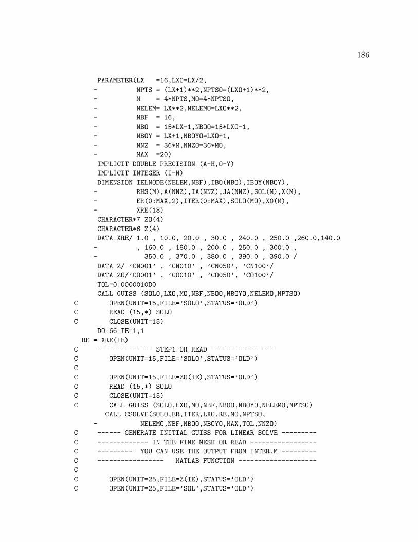
186
PARAMETER(LX =16,LXO=LX/2,- NPTS = (LX+1)**2,NPTSO=(LXO+1)**2,- M = 4*NPTS,MO=4*NPTSO,- NELEM= LX**2,NELEMO=LXO**2,- NBF = 16,- NBO = 15*LX-1,NBOO=15*LXO-1,- NBOY = LX+1,NBOYO=LXO+1,- NNZ = 36*M,NNZO=36*MO,- MAX =20)IMPLICIT DOUBLE PRECISION (A-H,O-Y)IMPLICIT INTEGER (I-N)DIMENSION IELNODE(NELEM,NBF),IBO(NBO),IBOY(NBOY),- RHS(M),A(NNZ),IA(NNZ),JA(NNZ),SOL(M),X(M),- ER(0:MAX,2),ITER(0:MAX),SOLO(MO),X0(M),- XRE(18)CHARACTER*7 ZO(4)CHARACTER*6 Z(4)DATA XRE/ 1.0 , 10.0, 20.0 , 30.0 , 240.0 , 250.0 ,260.0,140.0- , 160.0 , 180.0 , 200.0 , 250.0 , 300.0 ,- 350.0 , 370.0 , 380.0 , 390.0 , 390.0 /DATA Z/ ’CN001’ , ’CN010’ , ’CN050’, ’CN100’/DATA ZO/’CO001’ , ’CO010’ , ’CO050’, ’CO100’/TOL=0.0000010D0CALL GUISS (SOLO,LXO,MO,NBF,NBOO,NBOYO,NELEMO,NPTSO)
C OPEN(UNIT=15,FILE=’SOLO’,STATUS=’OLD’)C READ (15,*) SOLOC CLOSE(UNIT=15)
DO 66 IE=1,1RE = XRE(IE)
C -------------- STEP1 OR READ ----------------C OPEN(UNIT=15,FILE=’SOLO’,STATUS=’OLD’)CC OPEN(UNIT=15,FILE=ZO(IE),STATUS=’OLD’)C READ (15,*) SOLOC CLOSE(UNIT=15)C CALL GUISS (SOLO,LXO,MO,NBF,NBOO,NBOYO,NELEMO,NPTSO)
CALL CSOLVE(SOLO,ER,ITER,LXO,RE,MO,NPTSO,- NELEMO,NBF,NBOO,NBOYO,MAX,TOL,NNZO)
C ------ GENERATE INITIAL GUISS FOR LINEAR SOLVE ---------C ------------- IN THE FINE MESH OR READ -----------------C --------- YOU CAN USE THE OUTPUT FROM INTER.M ---------C ----------------- MATLAB FUNCTION --------------------CC OPEN(UNIT=25,FILE=Z(IE),STATUS=’OLD’)C OPEN(UNIT=25,FILE=’SOL’,STATUS=’OLD’)

187
C READ (25,*) SOLC CLOSE(UNIT=25)C CALL GUISS (SOL,LX,M,NBF,NBO,NBOY,NELEM,NPTS)
CALL GUISS (X0 ,LX,M,NBF,NBO,NBOY,NELEM,NPTS)C ------------- STEP2 ---------------------------
CALL FSOLVE(SOL,RE,SOLO,X0,- M,MO,LX,LXO,TOL,NPTS,NPTSO,NBF,- NBO,NBOY,NELEM,NELEMO,NBOO,- NBOYO,NNZ)
66 CONTINUEEND
C ----------------------------------------C THIS SUBROTINE WILL TAKE SOLO VECTOR AS THEC THE SOLUTION IN THE COARSE MESH AND COMPUTEC THE MATRIX A, IA, JA AND RHS AND SOLVE THEC LINEAR SYSTEM TO GENERATE THE VECTOR SOL ASC THE SOLUTION OF THE PROBLEM IN THE FINE MESHC ----------------------------------------
SUBROUTINE FSOLVE(SOL,RE,SOLO,X0,- M,MO,LX,LXO,TOL,NPTS,NPTSO,NBF,- NBO,NBOY,NELEM,NELEMO,NBOO,- NBOYO,NNZ)IMPLICIT DOUBLE PRECISION (A-H,O-Z)IMPLICIT INTEGER (I-N)DIMENSION SOL(M),SOLO(MO),IBO(NBO),IBOO(NBOO),- IBOY(NBOY),IBOYO(NBOYO),X0(M),Y0(M),- IELNODE(NELEM,NBF),IELNODEO(NELEMO,NBF),- EA(NBF,NBF),B(NBF,NBF,NBF),RHS(M),- A(NNZ),IA(NNZ),JA(NNZ),XX(M),YY(M),- PHI(NBF,6,4),XI(4),ETA(4),W(4)H=1.0D0/DBLE(FLOAT(LX))
CC HERE WE COMPUTE THE GLOBAL LABELING ARRAYC IELNODE FOR THE FINE MESH AND IELNODEO ARRAYC FOR THE COARSE MESH AND THE X-Y-COORDINATESC OF THE NODESC
CALL MAELNODE(IELNODE,IBO,IBOY,LX,- NBO,NBOY,NBF,M,NELEM,NPTS)CALL MAELNODE(IELNODEO,IBOO,IBOYO,LXO,- NBOO,NBOYO,NBF,MO,NELEMO,NPTSO)CALL COORD(XX,YY,LX,M)
CC HERE WE READ THE INTEGRATION POINTS XI(4)C AND ETA(4) AND W(4). ALSO WE READ THE ELEMENT

188
C STIFFNESS MATRIX A,IA,JA RESULTING FROM THE BIHARMONICC TERM AND THE ARRAY B(16,16,16) WHICH COMES FROM THEC TRILINEAR TERM IN THE STREAM FUNCTION FORMC
CALL SQUAD(XI,ETA,W)NBF2=NBF**2CALL MAEA(NBF,NBF2,EA)NBF3=NBF**3CALL MAB(NBF,NBF3,B)NBF4=6*4*NBFCALL MAQ(NBF,NBF4,PHI)CALL RZEROS(M,RHS)
CC HERE WE COMPUTE THE RHS VECTOR OF THEC LINEAR SYSTEMC
CALL RHS2L(RHS,LX,M,RE,NBF,IELNODE,- XX,YY,PHI,XI,ETA,W,NELEM,H)
CC HERE WE COMPUTE THE RESULTING MATRIXC
CALL FSTIFF(A,IA,JA,LX,RE,IELNODE,- XX,YY,LXO,IELNODEO,SOLO,EA,B,- NNZ,NBF,NELEM,NELEMO,M,MO,H,RHS)
CC HERE WE TAKE CARE THE BOUNDARY CONDITIONC SO CHANGE THE MATRIX A AND RHSC
CALL ATX(Y0,A,X0,IA,JA,NNZ,M)CALL AXPBY(RHS,1.0D0,RHS,-1.0D0,Y0,M)CALL FBOUNDRYA(A,IA,JA,IBO,IBOY,- NNZ,NBO,NBOY)CALL FBORHS(RHS,IBO,IBOY,M,NBO,NBOY,X0)
CC HERE WE SEND THE MATRIX AND RHS TO THEC LINEAR SOLVER BICGSTABC
CALL BICGSTAB(SOL,K,RHS,TOL,A,IA,JA,NNZ,M,1)CC HERE WE COMPUTE THE RESIDUAL = F( SOL )C
CALL ATX(X0,A,SOL,IA,JA,NNZ,M)CALL AXPBY(X0,1.0D0,RHS,-1.0D0,X0,M)CALL NORM(M,X0,RESDA)
C -----------

189
CALL FORCE(X0,LX,RE,SOL,- IELNODE,IBO,XX,YY,EA,B,PHI,W,XI,ETA,- M,NBF,NELEM,NBO)CALL FBORHS(X0,IBO,IBOY,M,NBO,NBOY,X0)CALL NORM(M,X0,RESDF)
C -----------CALL BACKUP(SOL,M,LX,LXO,RE,RESDA,RESDF,K)END
C ----------------------------------------SUBROUTINE RHS2L(RHS,LX,M,RE,NBF,IELNODE,- XX,YY,PHI,XI,ETA,W,NELEM,H)
CC THIS SUBROUTINE WILL COMPUTE THE RHS VECTORC OF THE LINEAR SYSTEM ON THE FINE MESHC
IMPLICIT DOUBLE PRECISION (A-H,O-Z)IMPLICIT INTEGER (I-N)DIMENSION RHS(M),IELNODE(NELEM,NBF),- XX(M),YY(M),PHI(NBF,6,4),- XI(4),ETA(4),W(4)DIMENSION X(4),Y(4)CALL RZEROS(M,RHS)DO 10 NK=1,NELEM
DO 20 II=1,4X(II) = XX( IELNODE(NK,II) )Y(II) = YY( IELNODE(NK,II) )
20 CONTINUEDO 30 IR=1,NBF
I=IELNODE(NK,IR)SUM1=0.0D0SUM2=0.0D0DO 40 IZ=1,4
S=H*(XI(IZ)+1.0D0)/2.0D0+X(1)T=H*(ETA(IZ)+1.0D0)/2.0D0+Y(1)CALL F1(VF1,S,T,RE)CALL F2(VF2,S,T,RE)SUM1=SUM1 + W(IZ)*PHI(IR,3,IZ)*VF1SUM2=SUM2 + W(IZ)*PHI(IR,2,IZ)*VF2
40 CONTINUEVALUE =SUM1 - SUM2RHS(I) = RHS(I) + VALUE*H/2.0D0
30 CONTINUE10 CONTINUE
ENDC ----------------------------------------
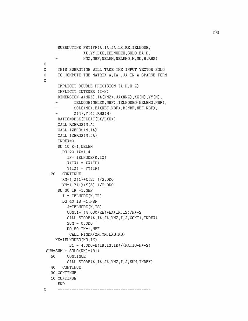
190
SUBROUTINE FSTIFF(A,IA,JA,LX,RE,IELNODE,- XX,YY,LXO,IELNODEO,SOLO,EA,B,- NNZ,NBF,NELEM,NELEMO,M,MO,H,RHS)
CC THIS SUBROTINE WILL TAKE THE INPUT VECTOR SOLOC TO COMPUTE THE MATRIX A,IA ,JA IN A SPARSE FORMC
IMPLICIT DOUBLE PRECISION (A-H,O-Z)IMPLICIT INTEGER (I-N)DIMENSION A(NNZ),IA(NNZ),JA(NNZ),XX(M),YY(M),- IELNODE(NELEM,NBF),IELNODEO(NELEMO,NBF),- SOLO(MO),EA(NBF,NBF),B(NBF,NBF,NBF),- X(4),Y(4),RHS(M)RATIO=DBLE(FLOAT(LX/LXO))CALL RZEROS(M,A)CALL IZEROS(M,IA)CALL IZEROS(M,JA)INDEX=0DO 10 K=1,NELEM
DO 20 IX=1,4IP= IELNODE(K,IX)X(IX) = XX(IP)Y(IX) = YY(IP)
20 CONTINUEXM=( X(1)+X(2) )/2.0D0YM=( Y(1)+Y(3) )/2.0D0
DO 30 IR =1,NBFI = IELNODE(K,IR)DO 40 IS =1,NBF
J=IELNODE(K,IS)CONT1= (4.0D0/RE)*EA(IR,IS)/H**2CALL STORE(A,IA,JA,NNZ,I,J,CONT1,INDEX)SUM = 0.0D0DO 50 IK=1,NBFCALL FINDK(XM,YM,LXO,KO)
KK=IELNODEO(KO,IK)B1 = 4.0D0*B(IR,IS,IK)/(RATIO*H**2)
SUM=SUM + SOLO(KK)*(B1)50 CONTINUE
CALL STORE(A,IA,JA,NNZ,I,J,SUM,INDEX)40 CONTINUE30 CONTINUE10 CONTINUE
ENDC ----------------------------------------
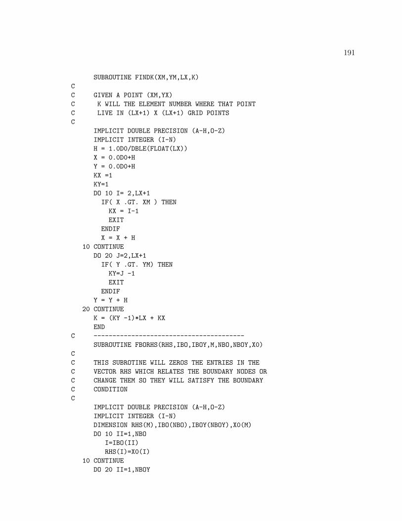
191
SUBROUTINE FINDK(XM,YM,LX,K)CC GIVEN A POINT (XM,YX)C K WILL THE ELEMENT NUMBER WHERE THAT POINTC LIVE IN (LX+1) X (LX+1) GRID POINTSC
IMPLICIT DOUBLE PRECISION (A-H,O-Z)IMPLICIT INTEGER (I-N)H = 1.0D0/DBLE(FLOAT(LX))X = 0.0D0+HY = 0.0D0+HKX =1KY=1DO 10 I= 2,LX+1
IF( X .GT. XM ) THENKX = I-1EXIT
ENDIFX = X + H
10 CONTINUEDO 20 J=2,LX+1
IF( Y .GT. YM) THENKY=J -1EXIT
ENDIFY = Y + H
20 CONTINUEK = (KY -1)*LX + KXEND
C ----------------------------------------SUBROUTINE FBORHS(RHS,IBO,IBOY,M,NBO,NBOY,X0)
CC THIS SUBROTINE WILL ZEROS THE ENTRIES IN THEC VECTOR RHS WHICH RELATES THE BOUNDARY NODES ORC CHANGE THEM SO THEY WILL SATISFY THE BOUNDARYC CONDITIONC
IMPLICIT DOUBLE PRECISION (A-H,O-Z)IMPLICIT INTEGER (I-N)DIMENSION RHS(M),IBO(NBO),IBOY(NBOY),X0(M)DO 10 II=1,NBO
I=IBO(II)RHS(I)=X0(I)
10 CONTINUEDO 20 II=1,NBOY
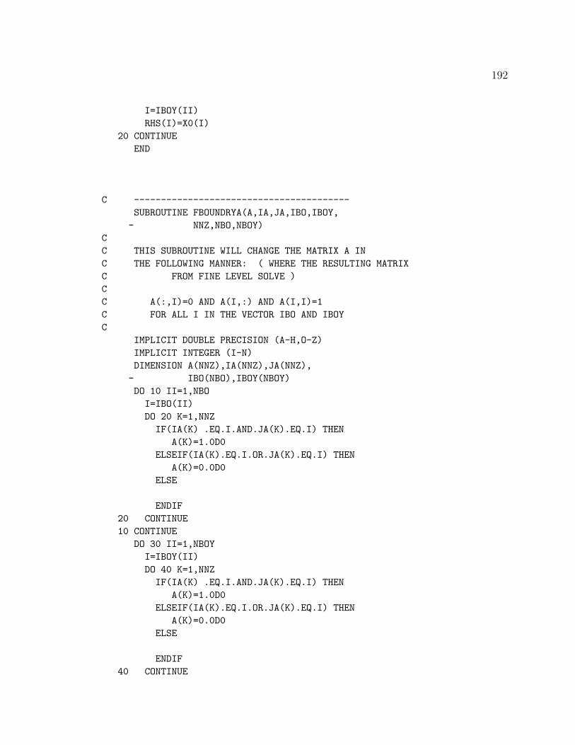
192
I=IBOY(II)RHS(I)=X0(I)
20 CONTINUEEND
C ----------------------------------------SUBROUTINE FBOUNDRYA(A,IA,JA,IBO,IBOY,- NNZ,NBO,NBOY)
CC THIS SUBROUTINE WILL CHANGE THE MATRIX A INC THE FOLLOWING MANNER: ( WHERE THE RESULTING MATRIXC FROM FINE LEVEL SOLVE )CC A(:,I)=0 AND A(I,:) AND A(I,I)=1C FOR ALL I IN THE VECTOR IBO AND IBOYC
IMPLICIT DOUBLE PRECISION (A-H,O-Z)IMPLICIT INTEGER (I-N)DIMENSION A(NNZ),IA(NNZ),JA(NNZ),- IBO(NBO),IBOY(NBOY)DO 10 II=1,NBO
I=IBO(II)DO 20 K=1,NNZ
IF(IA(K) .EQ.I.AND.JA(K).EQ.I) THENA(K)=1.0D0
ELSEIF(IA(K).EQ.I.OR.JA(K).EQ.I) THENA(K)=0.0D0
ELSE
ENDIF20 CONTINUE10 CONTINUE
DO 30 II=1,NBOYI=IBOY(II)DO 40 K=1,NNZ
IF(IA(K) .EQ.I.AND.JA(K).EQ.I) THENA(K)=1.0D0
ELSEIF(IA(K).EQ.I.OR.JA(K).EQ.I) THENA(K)=0.0D0
ELSE
ENDIF40 CONTINUE

193
30 CONTINUEEND
C -----------------------------------------SUBROUTINE CSOLVE(SOL,ER,ITER,LX,RE,M,NPTS,- NELEM,NBF,NBO,NBOY,MAX,TOL,NNZ)
CC THIS SUBROUTINE WILL SOLVE THE NAVIER-STOKESC EQUATION USING ONE LEVEL FINITE ELEMENT METHODC GIVING THE FOLLOWING :C LX = # OF SQUARES ALONG X-AXISC RE = REYNOLDS NUMBERC SOL = SOLUTION VECTOR (OUTPUT)C = INITIAL GUISS (INPUT)C ER(I,1) = I-TH RESIDUAL ERRORC ER(I,2) = NORM( SOL_I+1 - SOL_I )C ITER(I) = BICGSTAB ITERATION # NEEDED AT I-TH NEWTON STEPC THE OUTPUT SOLUTION IS STORED IN SOL AS BELOW :C SOL(1:NPTS) = PSI VALUES AT (LX+1)^2 POINTSC SOL(NPTS+1:2*NPTS) = PSI_X VALUES AT (LX+1)^2 POINTSC SOL(2*NPTS+1:3*NPTS) = PSI_Y VALUES AT (LX+1)^2 POINTSC SOL(3*NPTS+1:4*NPTS) = PSI_XY VALUES AT (LX+1)^2 POINTSC
IMPLICIT DOUBLE PRECISION (A-H,O-Z)IMPLICIT INTEGER (I-N)DIMENSION SOL(M),UP(M)DIMENSION IELNODE(NELEM,NBF),IBO(NBO),IBOY(NBOY),- XX(M),YY(M),PHI(NBF,6,4),B(NBF,NBF,NBF),- XI(4),ETA(4),W(4),EA(NBF,NBF),ER(0:MAX,2),- ITER(0:MAX),TSOL(M),TRHS(M),RHS(M),- A(NNZ),IA(NNZ),JA(NNZ)H=1.0D0/DBLE(FLOAT(LX))CALL MAELNODE(IELNODE,IBO,IBOY,LX,- NBO,NBOY,NBF,M,NELEM,NPTS)CALL COORD(XX,YY,LX,M)NBF4=6*4*NBFCALL MAQ(NBF,NBF4,PHI)CALL MAB(NBF,NBF**3,B)CALL SQUAD(XI,ETA,W)CALL MAEA(NBF,NBF**2,EA)CALL RZEROS(M,UP)CALL FORCE(RHS,LX,RE,SOL,- IELNODE,IBO,XX,YY,EA,B,PHI,W,XI,ETA,- M,NBF,NELEM,NBO)CALL BOUNDRYRHS(RHS,IBO,IBOY,- LX,NBF,NELEM,NBO,NBOY,NPTS,M)

194
CALL PNORM(M,RHS,XNORM,LX)
OLD = XNORM/DBLE(FLOAT(LX+1))ER(0,1) = OLDDO 10 I=1,MAX
CALL JACOBS(A,IA,JA,LX,RE,SOL,IELNODE,IBO,EA,B,- NNZ,M,NBF,NELEM,NBO,H)
CALL BOUNDRYA(A,IA,JA,IBO,IBOY,- NBO,NBOY,M,NNZ)
NWTN=ITOLB=0.00010D0CALL BICGSTAB(UP,K,RHS,TOL,A,IA,JA,NNZ,M,NWTN)ITER(I)=K;
CALL AXPBY(TSOL,1.0D0,SOL,-1.0D0,UP,M)CALL FORCE(TRHS,LX,RE,TSOL,
- IELNODE,IBO,XX,YY,EA,B,PHI,W,XI,ETA,- M,NBF,NELEM,NBO)
CALL BOUNDRYRHS(TRHS,IBO,IBOY,- LX,NBF,NELEM,NBO,NBOY,NPTS,M)
CALL PNORM(M,TRHS,XNORM,LX)XNEW = XNORM/DBLE(FLOAT(LX+1))CALL PNORM(M,UP,XNORM,LX)ER2 = XNORM/DBLE(FLOAT(LX+1))
IF( XNEW .GT. OLD ) THENCALL AXPBY(SOL,1.0D0,SOL,-0.50D0,UP,M)CALL FORCE(RHS,LX,RE,SOL,
- IELNODE,IBO,XX,YY,EA,B,PHI,W,XI,ETA,- M,NBF,NELEM,NBO)
CALL BOUNDRYRHS(RHS,IBO,IBOY,- LX,NBF,NELEM,NBO,NBOY,NPTS,M)
CALL PNORM(M,RHS,XNORM,LX)XNEW = XNORM/DBLE(FLOAT(LX+1))ER2= 0.50D0*ER2
PRINT*,’ I USE HALF STEP ’ELSE
CALL EQUAL(SOL,TSOL,M)CALL EQUAL(RHS,TRHS,M)
ENDIF
ER(I,1)= XNEW
195
ER(I,2)= ER2OLD = XNEW
C IP=1 FOR TEST AND IP=2 FOR CAVITYCALL BACKUPC(I,SOL,ER,ITER,MAX,M,LX,RE)IF(ER(I,1) .LT.TOL .AND. ER(I,2) .LT. TOL) EXIT
10 CONTINUEEND
C -----------------------------------------SUBROUTINE JACOBS(A,IA,JA,LX,RE,SOL,IELNODE,IBO,EA,B,- NNZ,M,NBF,NELEM,NBO,H)
CC THIS SUBROTINE WILL COMPUTE THE JACOBIAN MATRIX OF THEC PROBLEM AND STORE IT IN THREE VECTORS A , IA ,JA.C A = CONTAINS THE VALUES OF NONZERO ENTREE IN JACOBIANC IA = CONTAINS THE ROW LOCATION OF NONZERO ENTRIESC JA = CONTAINS THE COLUMN LOCATION OF NONZERO ENTRIESC
IMPLICIT DOUBLE PRECISION (A-H,O-Z)IMPLICIT INTEGER (I-N)DIMENSION A(NNZ),IA(NNZ),JA(NNZ),SOL(M),- IELNODE(NELEM,NBF),IBO(NBO),EA(NBF,NBF),- B(NBF,NBF,NBF)CALL RZEROS(NNZ,A)CALL IZEROS(NNZ,IA)CALL IZEROS(NNZ,JA)INDEX=0DO 10 K=1,NELEM
DO 20 IR =1,NBFI = IELNODE(K,IR)DO 30 IS =1,NBFJ=IELNODE(K,IS)CONT1 = (4.0D0/RE)*EA(IR,IS)/H**2CALL STORE(A,IA,JA,NNZ,I,J,CONT1,INDEX)SUM = 0.0D0DO 40 IK=1,NBF
KK=IELNODE(K,IK)BRACK = B(IR,IS,IK) + B(IR,IK,IS)
SUM=SUM + 4.0D0*SOL(KK)*BRACK/H**240 CONTINUE
CALL STORE(A,IA,JA,NNZ,I,J,SUM,INDEX)30 CONTINUE20 CONTINUE10 CONTINUE
END
196
C -----------------------------------------SUBROUTINE FORCE(RHS,LX,RE,SOL,- IELNODE,IBO,XX,YY,EA,B,PHI,W,XI,ETA,- M,NBF,NELEM,NBO)
CC THIS SUBROUTINE WILL TAKE THE INPUT VECTOR SOLC TO COMPUTE F( SOL ) AND STORE IT IN RHS VECTORC WHICH WILL BE THE RIGHT HAND SIDE OF THE RESULTINGC LINEAR SYSTEM FROM THE I-TH NEWTON ITERATION ANDC IN THE SAME TIME IT IS THE RESIDUAL.C
IMPLICIT DOUBLE PRECISION (A-H,O-Z)IMPLICIT INTEGER (I-N)DIMENSION RHS(M),SOL(M),IELNODE(NELEM,NBF),- IBO(NBO),XX(M),YY(M),EA(NBF,NBF),- B(NBF,NBF,NBF),PHI(NBF,6,4),- W(4),XI(4),ETA(4),X(4),Y(4)H=1.0D0/DBLE(FLOAT(LX))CALL RZEROS(M,RHS)DO 10 NK=1,NELEM
DO 20 II=1,4X(II) = XX( IELNODE(NK,II) )Y(II) = YY( IELNODE(NK,II) )
20 CONTINUEC ---------------------------------
DO 30 IR=1,NBFI=IELNODE(NK,IR)SUM1=0.0D0SUM2=0.0D0DO 40 IZ=1,4
S=H*(XI(IZ)+1.0D0)/2.0D0+X(1)T=H*(ETA(IZ)+1.0D0)/2.0D0+Y(1)CALL F1(VF1,S,T,RE)CALL F2(VF2,S,T,RE)SUM1=SUM1 + W(IZ)*PHI(IR,3,IZ)*VF1SUM2=SUM2 + W(IZ)*PHI(IR,2,IZ)*VF2
40 CONTINUEVALUE =-SUM1 + SUM2RHS(I) = RHS(I) + H*VALUE/2.0D0
C ----------------------------SUM=0.0D0DO 50 IS=1,NBF
J=IELNODE(NK,IS)SUM = SUM + (1.0D0/RE)*EA(IR,IS)*SOL(J)
50 CONTINUE

197
RHS(I) = RHS(I) + 4.0D0*SUM/H**2C -----------------------------
SUM=0.0D0DO 60 IS=1,NBF
J=IELNODE(NK,IS)DO 70 IK=1,NBFK= IELNODE(NK,IK)SUM=SUM+B(IR,IK,IS)*SOL(K)*SOL(J)
70 CONTINUE60 CONTINUE
RHS(I) = RHS(I) + 4.0D0*SUM/H**2C ---------------------------
30 CONTINUE10 CONTINUE
ENDC ------------------------------------
SUBROUTINE NORM(N,X,XNORM)CC THIS SUBROUTINE WILL COMPUTE THE EUCLIDEAN NORMC OF THE VECTOR X AND STORE IT IN XNORMC
IMPLICIT DOUBLE PRECISION (A-H,O-Z)IMPLICIT INTEGER (I-N)DIMENSION X(N)SUM = 0.0D0DO 10 I=1,N
SUM = SUM + X(I)**210 CONTINUE
XNORM = DSQRT( SUM )END
C ------------------------------------SUBROUTINE PNORM(N,X,XNORM,LX)
CC THIS SUBROUTINE WILL COMPUTE THE EUCLIDEANC NORM OF THE VECTOR X(1:4:N)C
IMPLICIT DOUBLE PRECISION (A-H,O-Z)IMPLICIT INTEGER (I-N)DIMENSION X(N)SUM = 0.0D0NPTS=(LX+1)**2M=4*NPTSDO 10 K=1,M,4
SUM = SUM + X(K)**210 CONTINUE
198
XNORM = DSQRT( SUM )END
SUBROUTINE RZEROS(N,X)IMPLICIT DOUBLE PRECISION (A-H,O-Z)IMPLICIT INTEGER (I-N)DIMENSION X(N)DO 10 I=1,NX(I) = 0.0D0
10 CONTINUEEND
SUBROUTINE IZEROS(N,IX)IMPLICIT DOUBLE PRECISION (A-H,O-Z)IMPLICIT INTEGER (I-N)DIMENSION IX(N)DO 10 I=1,N
IX(I) = 010 CONTINUE
END
SUBROUTINE BOUNDRYA(A,IA,JA,IBO,IBOY,- NBO,NBOY,M,NNZ)
CC THIS SUBROUTINE WILL CHANGE THE MATRIX A INC THE FOLLOWING MANNER: ( WHERE THE RESULTING MATRIXC FROM COARSE LEVEL SOLVE )CC A(:,I)=0 AND A(I,:) AND A(I,I)=1C FOR ALL I IN THE VECTOR IBO AND IBOYC
IMPLICIT DOUBLE PRECISION (A-H,O-Z)IMPLICIT INTEGER (I-N)DIMENSION A(NNZ),IA(NNZ),JA(NNZ),IBO(NBO),- IBOY(NBOY)DO 10 II=1,NBO
I=IBO(II)DO 20 K=1,NNZ
IF(IA(K) .EQ.I.AND.JA(K).EQ.I) THENA(K)=1.0D0
ELSEIF(IA(K).EQ.I.OR.JA(K).EQ.I) THENA(K)=0.0D0
ELSE
ENDIF

199
20 CONTINUE10 CONTINUE
DO 30 II=1,NBOYI=IBOY(II)DO 40 K=1,NNZ
IF(IA(K).EQ.I.AND.JA(K).EQ.I) THENA(K)=1.0D0
ELSEIF(IA(K).EQ.I.OR.JA(K).EQ.I) THENA(K)=0.0D0
ELSE
ENDIF40 CONTINUE30 CONTINUE
END
SUBROUTINE BOUNDRYRHS(RHS,IBO,IBOY,- LX,NBF,NELEM,NBO,NBOY,NPTS,M)
CC THIS SUBROTINE WILL ZEROS THE ENTRIES IN THEC VECTOR RHS WHICH RELATES THE BOUNDARY NODESC SO NO UPDATE IN THESE ENTRIES FOR EACH NEWTONC ITERATIONC
IMPLICIT DOUBLE PRECISION (A-H,O-Z)IMPLICIT INTEGER (I-N)DIMENSION RHS(M),IBO(NBO),IBOY(NBOY)DO 10 II=1,NBO
I=IBO(II)RHS(I)=0.0D0
10 CONTINUEDO 20 II=1,NBOY
I=IBOY(II)RHS(I)=0.0D0
20 CONTINUEEND
SUBROUTINE MAELNODE(IELNODE,IBO,IBOY,LX,- NBO,NBOY,NBF,M,NELEM,NPTS)
C -------------------------------C THIS SUBROUTINE COMPUTES THE ELEMENT NODE MATRIX OFC THE BOGNER-FOX ELEMENTS AND STORE THEM IN IELNODEC THE BOUNDARY POINTS AND STORE THEM IN IBO AND IBOY.
200
C POINTS.NOTE THAT THE DOMAIN IS [-1,1]X[-1,1].C LX = # OF SQYARES ALONG X-AXISC NELEM = # OF ELEMNTS = LX^2C NPTS = # OF POINTS = (LX+1)^2C H = 2.0 / LXC NBF = # OF BASIS FUNCTIONS IN EACH ELEMENT = 16C NBO = # OF BOUNDARY POINTS =C NNBO = # OF NORMAL BOUNDARYC ELNODE = EACH ROW CONTAINS THE GLOBAL NUMBERING OF LOCAL BASIS FNC.C IBO = CONTAINS ALL GLOBAL BOUNDARY NUMBERS EXCEPT THE TOPC WITH Y-DERIVATIVE NODEC IBOY = CONTAINS GLOBAL BOUNDARY NUMBERS ON THE TOP WITHC Y-DERIVATIVE NODECC NOTE : THE GLOBAL NUMBERING IS GOING FROM LOWER LEFT CORNERC TO THE TOP RIGHT CORNER STARTING BY LISTING THE FUNCTIONC NODE, X-DERIVATIVE NODE, Y-DERIVATIVE NODE ANDC XY-DERIVATIVE NODE FOR A POINT THEN LIST ALL NODESC FOR THE NEXT POINT AND SO ON.C -------------------------------
IMPLICIT DOUBLE PRECISION (A-H,O-Z)IMPLICIT INTEGER (I-N)DIMENSION IELNODE(NELEM,NBF),IBO(NBO),IBOY(NBOY)DO 10 I=1,LX
DO 20 J=1,LXIE = (I-1) * LX + JIK = (I-1)*(LX+1)+JK = 4*(IK-1) + 1IELNODE(IE,1) = KIELNODE(IE,2) = K+4IELNODE(IE,3) = K+4*(LX+1)IELNODE(IE,4) = K+4*(LX+2)IELNODE(IE,5) = IELNODE(IE,1)+1IELNODE(IE,6) = IELNODE(IE,2)+1IELNODE(IE,7) = IELNODE(IE,3)+1IELNODE(IE,8) = IELNODE(IE,4)+1IELNODE(IE,9) = IELNODE(IE,1)+2IELNODE(IE,10) = IELNODE(IE,2)+2IELNODE(IE,11) = IELNODE(IE,3)+2IELNODE(IE,12) = IELNODE(IE,4)+2IELNODE(IE,13) = IELNODE(IE,1)+3IELNODE(IE,14) = IELNODE(IE,2)+3IELNODE(IE,15) = IELNODE(IE,3)+3IELNODE(IE,16) = IELNODE(IE,4)+3
20 CONTINUE
201
10 CONTINUEC ---------------------------------C COMPUTE BOUNDARY NODEC ---------------------------------
N0 = 4*(LX+1)DO 30 I=1,N0IBO(I) = I30 CONTINUE
DO 40 J=1,LX+1K=4*LX*(LX+1)+4*(J-1)+1IBOY(J) = K+2IBO(N0+J)=KIBO(N0+LX+1+J)=K+1IBO(N0+2*(LX+1)+J)=K+3
40 CONTINUEN0=7*(LX+1)N1=11*(LX+1)-8DO 50 IKK=2,LX
IK1=IKK*(LX+1)IK2=(IKK-1)*(LX+1)+1K1=(IK1-1)*4+1K2=(IK2-1)*4+1IBO(N0+IKK-1)=K1IBO(N0+LX-2+IKK)=K1+1IBO(N0+2*(LX-1)+IKK-1)=K1+2IBO(N0+3*(LX-1)+IKK-1)=K1+3IBO(N1+IKK-1)=K2IBO(N1+LX-2+IKK)=K2+1IBO(N1+2*(LX-1)+IKK-1)=K2+2IBO(N1+3*(LX-1)+IKK-1)=K2+3
50 CONTINUEEND
SUBROUTINE COORD(X,Y,LX,M)CC THIS SUBROUTINE WILL COMPUTE THE X-COORDINATEC AND Y-COORDINATE OF ALL NODES AND STORE THEMC IN X AND Y ARRAY.C
IMPLICIT DOUBLE PRECISION (A-H,O-Z)IMPLICIT INTEGER (I-N)DIMENSION X(M),Y(M)NPTS = M/4H = 1.0D0/DBLE(FLOAT(LX))Y0 = 0.0D0
202
DO 10 I=1,LX+1X0 = 0.0D0DO 20 J=1,LX+1
IK = (I-1)*(LX+1) + JK=(IK-1)*4+1X(K)= X0Y(K)= Y0X(K+1)=X0X(K+2)=X0X(K+3)=X0Y(K+1)=Y0Y(K+2)=Y0Y(K+3)=Y0X0 = X0 + H
20 CONTINUEY0 = Y0 + H
10 CONTINUEEND
SUBROUTINE SQUAD(XI,ETA,W)CC THIS SUBROUTINE WILL RETURN THE INTEGRATIONC POINTS ON THE SQUARE [-1,1]X[-1,1] THEC X-COORDINATES OF THE POINTS ARE STORED INC ARRAY XI AND THE Y-COORDINATES STORED INC ARRAY ETA AND THE WIGHT ARE STORED IN WC
IMPLICIT DOUBLE PRECISION (A-H,O-Z)IMPLICIT INTEGER (I-N)DIMENSION XI(4),ETA(4),W(4)P = 1.0D0/DSQRT(3.0D0)PN = -PXI(1)=PNXI(2)=PXI(3)=PNXI(4)=PETA(1)=PNETA(2)=PNETA(3)=PETA(4)=PW(1)=1.0D0W(2)=1.0D0W(3)=1.0D0W(4)=1.0D0

203
END
SUBROUTINE MAQ(NBF,NBF4,Q)CC THIS SUBROTINE WILL READ THE FILE Q1C WHICH CONTAINS THE VALUES OF THE 16 BASISC FUNCTIONS, THE X-DERIVATIVE , Y-DERIVATIVEC XY-DERIVATIVE, XX-DERIVATIVE AND YY-DERIVATIVEC AND STORE THEM IN THE ARRAY Q( 16,6,4). THEC FIRST ARGUMENT OF Q REPRESENTS WHICH BASIS FUNCTIONSC THE SECOND ARGUMENT MEANS WHICH DERIVATIVE ANDC THE THIRD ARGUMENT REPRESENTS WHICH INTEGRATIONC POINTSC
IMPLICIT DOUBLE PRECISION (A-H,O-Y)IMPLICIT INTEGER (I-N)DIMENSION Q(NBF,6,4),Q1(NBF4)OPEN(UNIT=10,FILE=’Q1.DAT’,STATUS=’OLD’)DO 88 I=1,NBF4
READ (10,*) Q1(I)88 CONTINUE
DO 20 I=1,NBFDO 30 J=1,6DO 40 K=1,4N = (I-1)*24+(J-1)*4+KQ(I,J,K)=Q1(N)
40 CONTINUE30 CONTINUE20 CONTINUE
CLOSE(UNIT=10)END
SUBROUTINE MAEA(NBF,NBF2,EA)CC THIS SUBROUTINE WILL READ THE FILEC EA WHICH CONTAINS ALL VALUES OF POSSIBLEC INTEGRAL COMES FROM THE BIHARMONIC TERMC BETWEEN THE 16 BASIS FUNCTIONSC EA(I,J) = THE DOUBLE INTEGRAL OVER THEC THE SQUARE [-1.1]X[-1,1] OF THE PRODUCT OFC LAPLACE OF THE I-TH BASIS FUNCTION ANDC THE LAPLACE OF THE J-THE BASIS FUNCTIONC

204
IMPLICIT DOUBLE PRECISION (A-H,O-Z)IMPLICIT INTEGER (I-N)DIMENSION EA(NBF,NBF),IEA(NBF2)OPEN(UNIT=10,FILE=’EA.DAT’,STATUS=’OLD’)DO 99 I=1,NBF2
READ (10,*) IEA(I)99 CONTINUE
DO 20 I=1,NBFDO 30 J=1,NBFIP = (I-1)*16+JEA(I,J)=DBLE(FLOAT(IEA(IP)))/3150.0D0
30 CONTINUE20 CONTINUE
CLOSE(UNIT=10)END
SUBROUTINE MAB(NBF,NBF3,B)CC THIS SUBROUTINE WILL READ THE FILEC BB WHICH CONTAINS ALL VALUES OF POSSIBLEC INTEGRAL COMES FROM THE TRILINEAR TERMC BETWEEN THE 16 BASIS FUNCTIONS AND STOREC THEM IN THE ARRAY B(16,16,16).C B(I,J,K) = B( PHI_I ,PHI_J ,PHI_K)C
IMPLICIT DOUBLE PRECISION (A-H,O-Z)IMPLICIT INTEGER (I-N)DIMENSION B(NBF,NBF,NBF),IBB(NBF3)OPEN(UNIT=10,FILE=’BB.DAT’,STATUS=’OLD’)DO 99 I=1,NBF3
READ (10,*) IBB(I)99 CONTINUE
DO 20 I=1,NBFDO 30 J=1,NBFDO 40 K=1,NBFIP = (I-1)*256 + (J-1)*16 + KB(I,J,K)=DBLE(FLOAT(IBB(IP)))/88200.0D0
40 CONTINUE30 CONTINUE20 CONTINUE
CLOSE(UNIT=10)END
C -----------------------------------------SUBROUTINE BICGSTAB(X,K,B,TOL,C,IC,JC,NNZ,M,NWTN)
C

205
C THIS SUBROUTINE WILL SOLVE ANY LINEAR SYSTEM OFC EQUATION WITH THE RHS STORED IN B AND THE MATRIXC ARE STORED IN C , IC ,JC WHERE C CONTAINS ALL NONZEROC ENTRIES AND IC CONTAINS THE ROW LOCATION OF THE NONZEROC ENTRIES AND JC CONTAINS THE COLUMN LOCATION OF THEC NONZERO ENTRIES. THIS SUBROUTINE SOLVES THE LINEARC SYSTEM C X = B USING A BICGSTAB ALGORITHM.C THIS ALGORITHM IS DESCRIBED IN THE FOLLOWINGC REFERENCE:C T. CHAN J. DEMMEL J. DONATOR J. DONCARRA V. EIJKHOUTC R. POZO C. ROMINE R. BARRETT M.BERRY AND H. VAN DEV VORST.C , TEMPLATES: FOR THE SOLUTION OF LINEAR SYSTEMS:C BUILDING BLOCKS FOR ITERATIVE METHODS.C THE APPROXIMATION SOLUTION IS STORED IN THE VECTORC X(M) AND USE THIS X AS THE INITIAL GUISS.C
IMPLICIT DOUBLE PRECISION (A-H,O-Z)IMPLICIT INTEGER (I-N)DIMENSION X(M),B(M),C(NNZ),IC(NNZ),JC(NNZ)
C LOCALDIMENSION R(M),RH(M),P(M),V(M),S(M),T(M),UP(M)K=0CALL RZEROS(M,R)CALL RZEROS(M,RH)CALL RZEROS(M,P)CALL RZEROS(M,V)CALL RZEROS(M,S)CALL RZEROS(M,T)CALL RZEROS(M,UP)CALL ATX(R,C,X,IC,JC,NNZ,M)CALL AXPBY(R,1.0D0,B,-1.0D0,R,M)CALL EQUAL(RH,R,M)DO 10 I=1,10*M*M
CALL DOT(ROW,RH,R,M)IF(ROW .EQ. 0.0D0 ) EXITIF(I .EQ. 1) THENCALL EQUAL(P,R,M)
ELSEBETA = (ROW/ROWOLD)*(ALPHA/W)CALL AXPBY(P,BETA,P,-BETA*W,V,M)CALL AXPBY(P,1.0D0,R,1.0D0,P,M)
ENDIFCALL ATX(V,C,P,IC,JC,NNZ,M)CALL DOT(VAL,RH,V,M)ALPHA = ROW/VAL

206
CALL AXPBY(S,1.0D0,R,-ALPHA,V,M)CALL NORM(M,S,XNORM)IF( XNORM .LT. TOL) THEN
K=ICALL AXPBY(X,1.0D0,X,ALPHA,P,M)PRINT*,’I STOP BECAUSE NORM(S)<TOL’,NWTN,KEXIT
ENDIFCALL ATX(T,C,S,IC,JC,NNZ,M)CALL DOT(VAL2,T,S,M)CALL DOT(VAL3,T,T,M)W = VAL2/VAL3CALL AXPBY(UP,ALPHA,P,W,S,M)CALL AXPBY(X,1.0D0,X,1.0D0,UP,M)CALL AXPBY(R,1.0D0,S,-W,T,M)IF(W .EQ. 0.0D0 ) THEN
PRINT*,’I CAN NOT CONTINUE ITERATION BECAUSE W = 0’EXIT
ENDIFCALL NORM(M,UP,XUP)CALL NORM(M,R,XR)IF( XUP .LT. TOL .AND. XR .LT. TOL ) THENK = IPRINT*,’I STOP BECAUSE NORM(R,UP)<TOL’,NWTN,KEXIT
END IFROWOLD=ROW
10 CONTINUEEND
C-------------------------------SUBROUTINE DOT(VAL,X,Y,M)
CC THIS SUBROUTINE COMPUTES THE DOT PRODUCTC BETWEEN THE TWO VECTORS X AND YC
INTEGER I,MDOUBLE PRECISION X(M),Y(M),VALVAL = 0.0D0DO 10 I=1,M
VAL = VAL + X(I)*Y(I)10 CONTINUE
ENDC
SUBROUTINE EQUAL(X,Y,M)
207
DOUBLE PRECISION X(M),Y(M)INTEGER M,IDO 10 I=1,M
X(I) = Y(I)10 CONTINUE
ENDCC
SUBROUTINE AXPBY(Z,ALPHA,X,BETA,Y,M)CC THIS SUBROUTINE WILL DO THE FOLLOWING ;C Z = ALPHA * X + BETA * YC WHERE ALPHA AND BETA ARE CONSTANTSC AND X,Y,Z ARE VECTORSC
IMPLICIT DOUBLE PRECISION (A-H,O-Z)IMPLICIT INTEGER (I-N)DIMENSION Z(M),X(M),Y(M)DO 10 I=1,M
Z(I) = ALPHA*X(I) + BETA*Y(I)10 CONTINUE
ENDCCC----------------------------------
SUBROUTINE ATX(Y,A,X,IA,JA,NNZ,M)CC THIS SUBROTINE WILL DO MATRIX-VECTOR MULTIPLICATIONC BETWEEN THE MATRIX (A,IA,JA) AND THE VECTOR X ANDC STORE THE RESULT IN THE VECTOR Y WHERE A ARE STORED INC SPARSE FORM (I.E)C A CONTAINS ALL NONZERO ENTRIES ANDC IA CONTAINS THE ROW LOCATION OF THE NONZERO ENTRIES ANDC JA CONTAINS THE COLUMN LOCATION OF THE NONZERO ENTRIES.C
IMPLICIT DOUBLE PRECISION (A-H,O-Z)IMPLICIT INTEGER (I-N)DIMENSION IA(NNZ),JA(NNZ)DIMENSION X(M),Y(M),A(NNZ)CALL RZEROS(M,Y)DO 10 K=1,NNZ
I=IA(K)J=JA(K)AIJ=A(K)Y(I)= Y(I) + AIJ*X(J)

208
10 CONTINUEEND
SUBROUTINE STORE(A,IA,JA,NNZ,IROW,JCOL,AIJ,INDEX)CC THIS SUBROUTINE WILL STORE ANY ELEMENT CONTRIBUTIONC AIJ TO THE JACOBIAN OR THE FINE LEVEL MATRIX IN A IA JA.C
IMPLICIT DOUBLE PRECISION (A-H,O-Z)IMPLICIT INTEGER (I-N)DIMENSION A(NNZ),IA(NNZ),JA(NNZ)CALL CHK(NNZ,IA,JA,IROW,JCOL,IFLAG,INDEX)IF( IFLAG .EQ. 0) THEN
INDEX = INDEX + 1A(INDEX) = AIJIA(INDEX) = IROWJA(INDEX) = JCOL
ELSEA(IFLAG) = A(IFLAG) + AIJ
ENDIFEND
SUBROUTINE CHK(NNZ,IA,JA,IROW,JCOL,IFLAG,INDEX)CC THIS SUBROUTINE WILL CHECK IF THIS A(IROW , JCOL)C HAVE BEEN ENTERED IN A IA JA BEFORE OR NOT.C
IMPLICIT INTEGER (I-N)DIMENSION IA(NNZ),JA(NNZ)IFLAG = 0DO 10 I=1,INDEX
IF( IA(I) .EQ. IROW .AND. JA(I) .EQ. JCOL ) THENIFLAG = I
EXITENDIF
10 CONTINUEEND
SUBROUTINE NAME(RE,LX,LXO,F)CC THIS SUBROTINE WILL GIVE A FILE NAME WITHC THE HELP OF RE,LX,LXO AND STORES THE NAMEC IN F.CCHARACTER*10 NO

209
CHARACTER*11 FDOUBLE PRECISION RE
NO(1:10)=’1234567890’C --------------------------------
J=REK4=J/1000J3=J-K4*1000K3=J3/100J2= J-K3*100K2=J2/10J1=J2-10*K2K1=J1IF(K1 .EQ. 0) K1=10IF(K2 .EQ. 0) K2=10IF(K3 .EQ. 0) K3=10IF(K4 .EQ. 0) K4=10
C --------------------------------LX2=LX/10LX1=LX-LX2*10IF(LX1 .EQ. 0) LX1=10IF(LX2 .EQ. 0) LX2=10
C --------------------------------LXO2=LXO/10LXO1=LXO-LXO2*10IF(LXO1 .EQ. 0) LXO1=10IF(LXO2 .EQ. 0) LXO2=10
C --------------------------------F=’R’//NO(K4:K4)//NO(K3:K3)//NO(K2:K2)//NO(K1:K1)//
- ’H’//NO(LX2:LX2)//NO(LX1:LX1)//- ’H’//NO(LXO2:LXO2)//NO(LXO1:LXO1)END
SUBROUTINE BACKUP(SOL,M,LX,LXO,RE,RESDA,RESDF,K)CC THIS SUBROUTINE WILL PRINT THE SOLUTION AND SOMEC STATISTICS TO A FILE NAME GENERATED BY NAME SUBROUTINEC
IMPLICIT DOUBLE PRECISION (A-H,O-Y)IMPLICIT INTEGER (I-N)DIMENSION SOL(M)CHARACTER*11 ZCALL NAME(RE,LX,LXO,Z)OPEN(UNIT=10,FILE=Z,STATUS=’NEW’)WRITE (10,*) ’CAVITY PROBLEM WITH 2-LEVEL’WRITE (10,*) ’LX = ’,LX,’ LXO = ’,LXO
210
WRITE (10,*) ’RE = ’,REWRITE (10,*) ’# OF ITERATIONS = ’,KWRITE (10,*) ’ RESIDUAL(B-AX) = ’, RESDAWRITE (10,*) ’ RESIDUAL F(X) = ’, RESDFWRITE (10,*) ’ ---------------------------- ’DO 30 J=1,M
WRITE(10,*) SOL(J)30 CONTINUE
CLOSE(UNIT=10)
END
SUBROUTINE BACKUPC(I,SOL,ER,ITER,MAX,M,LX,RE)CC THIS SUBROUTINE WILL PRINT THE SOLUTION AND SOMEC STATISTICS TO A FILE NAME GENERATED BY NAME SUBROUTINEC
IMPLICIT DOUBLE PRECISION (A-H,O-Y)IMPLICIT INTEGER (I-N)DIMENSION SOL(M),ER(0:MAX,2),ITER(0:MAX)CHARACTER*10 ZF
CALL NAMEC(RE,LX,I,ZF)OPEN(UNIT=22,FILE=ZF,STATUS=’NEW’)
WRITE(22,*) ’LX = ’,LX,’ RE = ’,REDO 40 K=0,I
WRITE(22,*) K,ITER(K),ER(K,1),ER(K,2)40 CONTINUE
DO 30 J=1,MWRITE(22,*) SOL(J)
30 CONTINUECLOSE(UNIT=20)END
C --------------------------------SUBROUTINE NAMEC(RE,LX,ITER,F)
CC THIS SUBROTINE WILL GIVE A FILE NAME WITHC THE HELP OF RE,LX,LXO AND STORES THE NAMEC IN F.CCHARACTER*10 NO
CHARACTER*10 FDOUBLE PRECISION RE
NO(1:10)=’1234567890’
211
C --------------------------------J=REK3=J/100J2= J-K3*100K2=J2/10J1=J2-10*K2K1=J1IF(K1 .EQ. 0) K1=10IF(K2 .EQ. 0) K2=10IF(K3 .EQ. 0) K3=10
C --------------------------------LX2=LX/10LX1=LX-LX2*10IF(LX1 .EQ. 0) LX1=10IF(LX2 .EQ. 0) LX2=10
C --------------------------------IT2=ITER/10IT1=ITER-IT2*10IF(IT1 .EQ. 0) IT1=10IF(IT2 .EQ. 0) IT2=10
C --------------------------------F=’R’//NO(K3:K3)//NO(K2:K2)//NO(K1:K1)//
- ’X’//NO(LX2:LX2)//NO(LX1:LX1)//- ’I’//NO(IT2:IT2)//NO(IT1:IT1)END
C ----------------------------CC THE FOLLOWING SUBROUTINES AFTER THIS LINEC ARE NOT GENERAL SUBROUTINES. SOME OF THEMC ARE FOR THE TEST PROBELEM WITH A KNOWN SOLUTIONC AND THE OTHER ARE FOR CAVITY FLOW PROBELM.C THE REST IS FOR DIFFRENT WAY OF GLOBAL ORDERING.CC NOTE :C 1-FOR TEST PROBLEM :C COMPILE THE ABOVE LINES WITH F1(TEST) ANDC F2(TEST) AND GUISS(TEST)C 2-FOR CAVITY PROBLEM :C COMPILE THE ABOVE LINES WITH F1(CAVITY) ANDC F2(CAVITY) AND GUISS(CAVITY)C 3-FOR ANY OTHER PROBLEM WITH [0,1]^2 DOMAINC CHANGE SOME LINES IN MAELNODE SUBROUTINEC TO COMPUTE IBOY ARRAY. IBOY CONTAINS NONHOMOG.C BOUNDARY CONDITIONS ANDC SUPPLY F1 , F2 AND GUISS WHERE F1 AND F2
212
C BODY FORCE FUNCTION OF NSE. SUPPLY GUISS SUBROUTINEC WHICH GENERATE A VECTOR. THIS VECTOR SATISFY THEC BOUNDARY CONDITIONS OF THE PROBLEM AND THE OTHERC ENTRIES OF THE VECTOR ARE ZEROS. THEN COMPILEC THE ABOVE AFTER CHANGE WITH THE NEW MAELNODE, F1C F2 AND GUISSC 4-FOR ANY GENERAL PROBLEMC REWRITE MAELNODE , COORD , F1 , F2 AND GUISSC THEN COMPILE THE ABOVE WITH THESE NEW ONES AFTERC YOU DELETE COORD AND MAELNODE FROM ABOVECCCC
SUBROUTINE F1(FF,X,Y,RE)CC THIS SUBROUTINE COMPUTE THE FIRST COMPONENT OFC THE BODY FORCE FUNCTION IN THE NAVIER-STOKES EQUATIONSC IN PARTICULAR , IT IS F1(X,Y) AFTER WE SUBSTITUTEC THE STREAM FUNCTION PSI(X,Y) TO BEC X^2 * ( X - 1)^2 * Y * (Y - 1)^2C (TEST)C
IMPLICIT DOUBLE PRECISION (A-H,O-Z)IMPLICIT INTEGER (I-N)FF=X**2*(3 + 64*(-1 + X)**7*X**5*(-1 + 2*X)*- (1 - 2*Y)**2*(-1 + Y)**6*Y**6 +- 16*(1 - 2*X)*(-1 + X)**7*X**5*(-1 + Y)**6*Y**6*- (3 - 14*Y + 14*Y**2) -- (8*(-1 + X)**2*Y*(1 - 3*Y + 2*Y**2)*- (6*(-1 + Y)**2*Y**2 -- 28*X*(-1 + Y)**2*Y**2 -- 6*X**3*(1 - 7*Y + 7*Y**2) +- 3*X**4*(1 - 7*Y + 7*Y**2) +- X**2*(3 - 21*Y + 49*Y**2 - 56*Y**3 +- 28*Y**4)))/RE)END
SUBROUTINE F2(FF,X,Y,RE)CC THIS SUBROUTINE COMPUTE THE SECOND COMPONENT OFC THE BODY FORCE FUNCTION IN THE NAVIER-STOKES EQUATIONSC IN PARTICULAR , IT IS F1(X,Y) AFTER WE SUBSTITUTE

213
C THE STREAM FUNCTION PSI(X,Y) TO BEC X^2 * ( X - 1)^2 * Y * (Y - 1)^2C (TEST)C
IMPLICIT DOUBLE PRECISION (A-H,O-Z)IMPLICIT INTEGER (I-N)FF=Y**2*(3 + 64*(1 - 2*X)**2*(-1 + X)**6*X**6*- (-1 + Y)**7*Y**5*(-1 + 2*Y) -- 16*(-1 + X)**6*X**6*(3 - 14*X + 14*X**2)*- (-1 + Y)**7*Y**5*(-1 + 2*Y) +- (8*X*(1 - 3*X + 2*X**2)*(-1 + Y)**2*- (3*(-1 + Y)**2*Y**2 -- 21*X*(-1 + Y)**2*Y**2 -- 4*X**3*(3 - 14*Y + 14*Y**2) +- X**4*(6 - 28*Y + 28*Y**2) +- X**2*(6 - 28*Y + 49*Y**2 - 42*Y**3 +- 21*Y**4)))/RE)END
SUBROUTINE GUISS (X0,LX,M,NBF,NBO,NBOY,NELEM,NPTS)CC THIS SUBROTINE WILL PICK AN INITIAL GUISS WHICHC SATISFIES THE BOUNDARY CONDITION OF THE PROBLEMSC THIS INITIAL GUISS IS SUITABLE TO BE THE INITIALC GUISS FOR THE NEWTON ITERATIONC (TEST)C
IMPLICIT DOUBLE PRECISION (A-H,O-Z)IMPLICIT INTEGER (I-N)DIMENSION X0(M),IBO(NBO),IBOY(NBOY),IELNODE(NELEM,NBF)CALL RZEROS(M,X0)ENDSUBROUTINE F1(FF,X,Y,RE)
CC THIS SUBROUTINE COMPUTE THE FIRST COMPONENT OFC THE BODY FORCE FUNCTION IN THE NAVIER-STOKES EQUATIONSC (CAVITY)C
IMPLICIT DOUBLE PRECISION (A-H,O-Z)IMPLICIT INTEGER (I-N)FF=0.0D0END
214
SUBROUTINE F2(FF,X,Y,RE)CC THIS SUBROUTINE COMPUTE THE SECOND COMPONENT OFC THE BODY FORCE FUNCTION IN THE NAVIER-STOKES EQUATIONSC (CAVITY)C
IMPLICIT DOUBLE PRECISION (A-H,O-Z)IMPLICIT INTEGER (I-N)FF=0.0D0END
SUBROUTINE GUISS (X0,LX,M,NBF,NBO,NBOY,NELEM,NPTS)CC THIS SUBROTINE WILL PICK AN INITIAL GUISS WHICHC SATISFIES THE BOUNDARY CONDITION OF THE PROBLEMSC THIS INITIAL GUISS IS SUITABLE TO BE THE INITIALC GUISS FOR THE NEWTON ITERATION (CAVITY PROBLEM)C
IMPLICIT DOUBLE PRECISION (A-H,O-Z)IMPLICIT INTEGER (I-N)DIMENSION X0(M),IBO(NBO),IBOY(NBOY),IELNODE(NELEM,NBF)CALL MAELNODE(IELNODE,IBO,IBOY,LX,- NBO,NBOY,NBF,M,NELEM,NPTS)CALL RZEROS(M,X0)DO 10 II=1,NBOY
I=IBOY(II)X0(I) = 1.0D0
10 CONTINUEEND
CC BELOW THIS LINE FOR DIFFRENT GLOBAL ORDERINGC
SUBROUTINE PNORM(N,X,XNORM,K)CC THIS SUBROUTINE WILL COMPUTE THE EUCLIDEANC NORM OF THE VECTOR X(1:K)C
IMPLICIT DOUBLE PRECISION (A-H,O-Z)IMPLICIT INTEGER (I-N)DIMENSION X(N)SUM = 0.0D0DO 10 I=1,K

215
SUM = SUM + X(I)**210 CONTINUE
XNORM = DSQRT( SUM )ENDSUBROUTINE MAELNODE(IELNODE,IBO,IBOY,LX,- NBO,NBOY,NBF,M,NELEM,NPTS)
C -------------------------------C THIS SUBROUTINE COMPUTES THE ELEMENT NODE MATRIX OFC THE BOGNER-FOX ELEMENTS AND STORE THEM IN IELNODEC THE BOUNDARY POINTS AND STORE THEM IN IBO AND IBOY.C POINTS.NOTE THAT THE DOMAIN IS [-1,1]X[-1,1].C LX = # OF SQYARES ALONG X-AXISC NELEM = # OF ELEMNTS = LX^2C NPTS = # OF POINTS = (LX+1)^2C H = 2.0 / LXC NBF = # OF BASIS FUNCTIONS IN EACH ELEMENT = 16C NBO = # OF BOUNDARY POINTS =C NNBO = # OF NORMAL BOUNDARYC ELNODE = EACH ROW CONTAINS THE GLOBAL NUMBERING OF LOCAL BASIS FNC.C IBO = CONTAINS ALL GLOBAL BOUNDARY NUMBERS EXCEPT THE TOPC WITH Y-DERIVATIVE NODEC IBOY = CONTAINS GLOBAL BOUNDARY NUMBERS ON THE TOP WITHC Y-DERIVATIVE NODECC NOTE : THE GLOBAL NUMBERING IS GOING FROM LOWER LEFT CORNERC TO THE TOP RIGHT CORNER STARTING BY LISTING THE FUNCTIONC NODE THEN X-DERIVATIVE NODE THEN Y-DERIVATIVE NODE THENC XY-DERIVATIVE NODE.C -------------------------------
IMPLICIT DOUBLE PRECISION (A-H,O-Z)IMPLICIT INTEGER (I-N)DIMENSION IELNODE(NELEM,NBF),IBO(NBO),IBOY(NBOY)N0 = 0DO 10 I=1,LX
DO 20 J=1,LXIE = (I-1) * LX + JK = IE + N0IELNODE(IE,1) = KIELNODE(IE,2) = K+1IELNODE(IE,3) = K+1+LXIELNODE(IE,4) = K+2+LXIELNODE(IE,5) = K+NPTSIELNODE(IE,6) = K+NPTS+1IELNODE(IE,7) = K+LX+1+NPTSIELNODE(IE,8) = K+LX+2+NPTS

216
IELNODE(IE,9) = K+2*NPTSIELNODE(IE,10) = K+2*NPTS+1IELNODE(IE,11) = K+LX+1+2*NPTSIELNODE(IE,12) = K+LX+2+2*NPTSIELNODE(IE,13) = K+3*NPTSIELNODE(IE,14) = K+1+3*NPTSIELNODE(IE,15) = K+LX+1+3*NPTSIELNODE(IE,16) = K+LX+2+3*NPTS
20 CONTINUEN0 = N0 + 1
10 CONTINUEC ---------------------------------C COMPUTE BOUNDARY NODEC ---------------------------------
DO 30 I=1,LX-1IBO(I) = I+1IBO(I+LX-1) = (LX+1)*LX + I + 1
30 CONTINUEDO 40 I=1,LX+1
IBO(2*LX-2+I) = (I-1)*(LX + 1) + 1IBO(3*LX-1+I) = I*(LX + 1)
40 CONTINUEC ---------------------------------C COMPUTE NORMAL BOUNDARY NODEC ---------------------------------
DO 50 I=1,4*LXIX=I+4*LXIXY=I+8*LXIBO(IX) = IBO(I) + NPTSIBO(IXY) = IBO(I) + 3*NPTS
50 CONTINUEDO 60 I=1,LX+1
IY=I+12*LXIBO(IY) = I + 2*NPTS
60 CONTINUEDO 70 I=2,LX
IY = I + 13*LXIBO(IY) = I*(LX+1) + 2*NPTS
70 CONTINUEDO 80 I=2,LX
IY = I - 1 + 14*LXIBO(IY) = (I-1)*(LX+1) + 1
80 CONTINUEDO 90 I=0,LX
IBOY(I+1)= 3*NPTS - I
217
90 CONTINUEEND
SUBROUTINE COORD(X,Y,LX,M)CC THIS SUBROUTINE WILL COMPUTE THE X-COORDINATEC AND Y-COORDINATE OF ALL NODES AND STORE THEMC IN X AND Y ARRAY.C
IMPLICIT DOUBLE PRECISION (A-H,O-Z)IMPLICIT INTEGER (I-N)DIMENSION X(M),Y(M)NPTS = M/4H = 2.0D0/DBLE(FLOAT(LX))Y0 = -1.0D0DO 10 I=1,LX+1
X0 = -1.0D0DO 20 J=1,LX+1
IP = (I-1)*(LX+1) + JX(IP)= X0Y(IP)= Y0X0 = X0 + H
20 CONTINUEY0 = Y0 + H
10 CONTINUEDO 30 I=1,NPTS
IX=I+NPTSIY=I+2*NPTSIXY=I+3*NPTSX(IX) = X(I)X(IY) = X(I)X(IXY) = X(I)Y(IX) = Y(I)Y(IY) = Y(I)Y(IXY) = Y(I)
30 CONTINUEEND
SUBROUTINE FINDK(XM,YM,LX,K)CC GIVEN A POINT (XM,YX)C K WILL THE ELEMENT NUMBER WHERE THAT POINTC LIVE IN (LX+1) X (LX+1) GRID POINTSC
IMPLICIT DOUBLE PRECISION (A-H,O-Z)
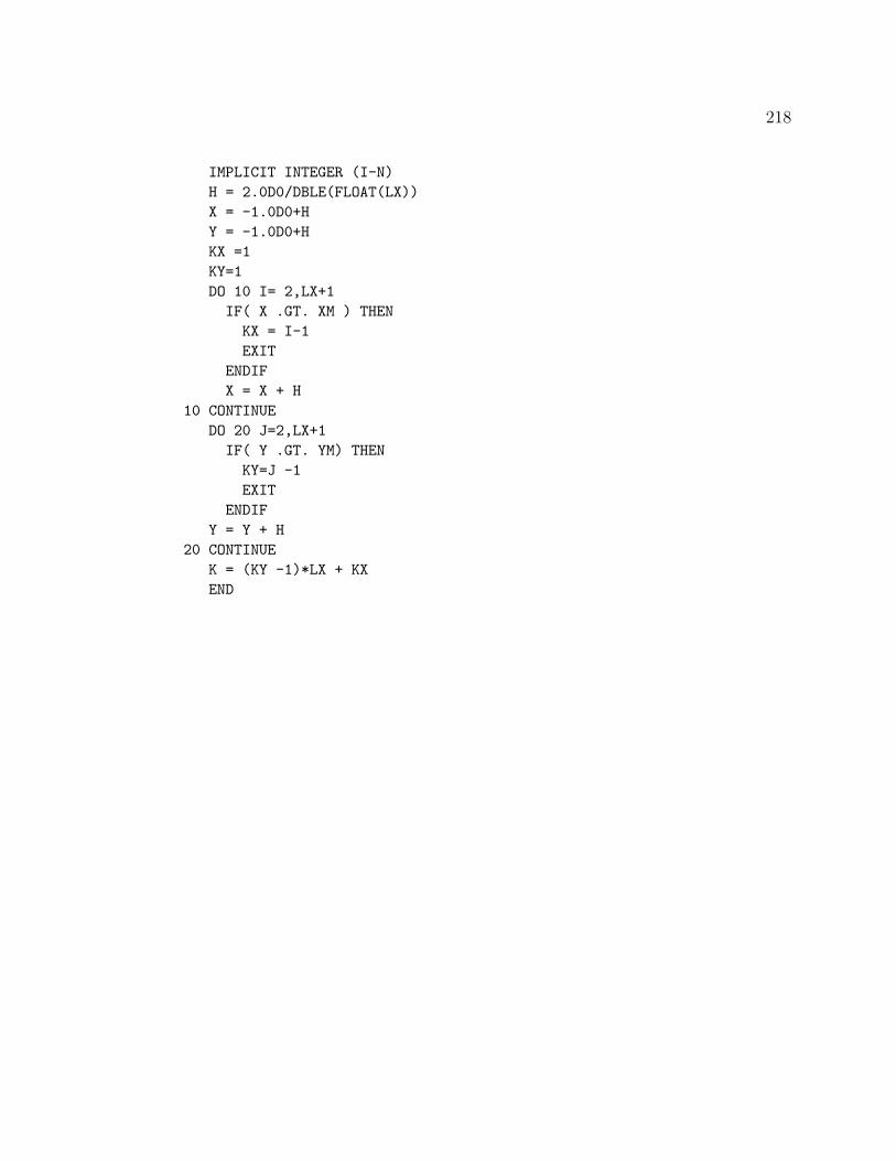
218
IMPLICIT INTEGER (I-N)H = 2.0D0/DBLE(FLOAT(LX))X = -1.0D0+HY = -1.0D0+HKX =1KY=1DO 10 I= 2,LX+1
IF( X .GT. XM ) THENKX = I-1EXIT
ENDIFX = X + H
10 CONTINUEDO 20 J=2,LX+1
IF( Y .GT. YM) THENKY=J -1EXIT
ENDIFY = Y + H
20 CONTINUEK = (KY -1)*LX + KXEND
Appendix C
MATLAB and M-files
219
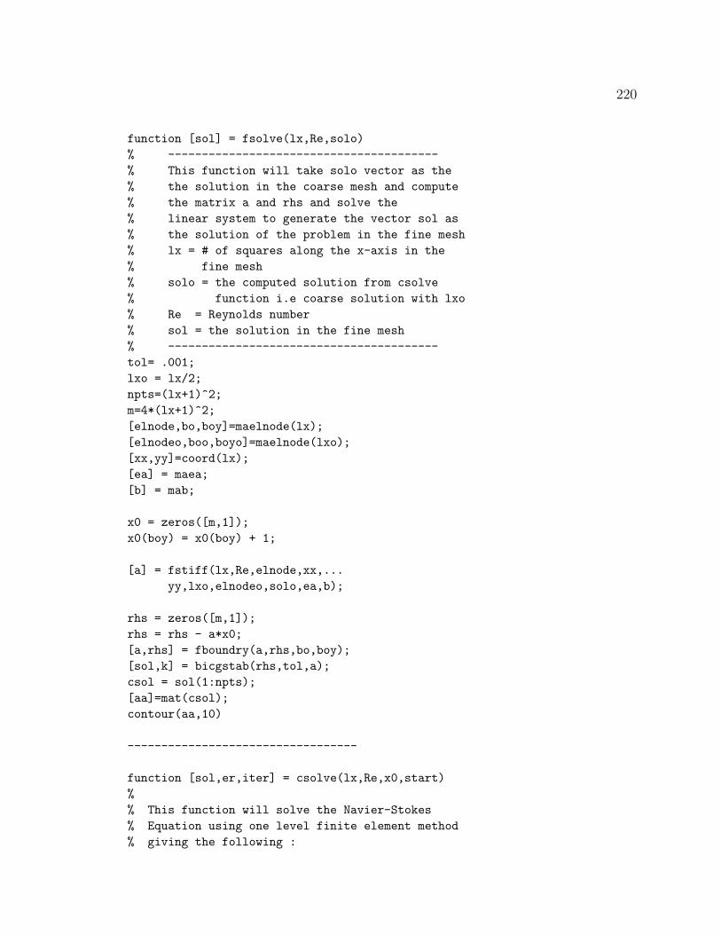
220
function [sol] = fsolve(lx,Re,solo)% ----------------------------------------% This function will take solo vector as the% the solution in the coarse mesh and compute% the matrix a and rhs and solve the% linear system to generate the vector sol as% the solution of the problem in the fine mesh% lx = # of squares along the x-axis in the% fine mesh% solo = the computed solution from csolve% function i.e coarse solution with lxo% Re = Reynolds number% sol = the solution in the fine mesh% ----------------------------------------tol= .001;lxo = lx/2;npts=(lx+1)^2;m=4*(lx+1)^2;[elnode,bo,boy]=maelnode(lx);[elnodeo,boo,boyo]=maelnode(lxo);[xx,yy]=coord(lx);[ea] = maea;[b] = mab;
x0 = zeros([m,1]);x0(boy) = x0(boy) + 1;
[a] = fstiff(lx,Re,elnode,xx,...yy,lxo,elnodeo,solo,ea,b);
rhs = zeros([m,1]);rhs = rhs - a*x0;[a,rhs] = fboundry(a,rhs,bo,boy);[sol,k] = bicgstab(rhs,tol,a);csol = sol(1:npts);[aa]=mat(csol);contour(aa,10)
----------------------------------
function [sol,er,iter] = csolve(lx,Re,x0,start)%% This function will solve the Navier-Stokes% Equation using one level finite element method% giving the following :

221
% lx = # of squares along x-axis% Re = Reynolds number% x0 = initial guiss% start = Newton iteration number% sol = solution vector% er(i,1) = i-th residual error% er(i,2) = norm( sol_i+1 - sol_i )% iter(i) = BICGSTAB iteration # needed at i-th Newton step% The output solution is stored in sol as below :% sol(1:npts) = psi values at (lx+1)^2 points% sol(npts+1:2*npts) = psi_x values at (lx+1)^2 points% sol(2*npts+1:3*npts) = psi_y values at (lx+1)^2 points% sol(3*npts+1:4*npts) = psi_xy values at (lx+1)^2 points%h=2/lx;tol= 1e-6;max=20;npts=(lx+1)^2;m=4*(lx+1)^2;[elnode,bo,boy]=maelnode(lx);[xx,yy]=coord(lx);[ea] = maea;[b] = mab;sol = x0;%load solup=zeros([m,1]);er1=1e10;for i=start:max
[a] = jacobs(lx,Re,sol,elnode,bo,ea,b);[rhs] = force(lx,Re,sol,elnode,bo,xx,yy,ea,b);[a,rhs] = boundry(a,rhs,bo,boy);older1=er1;er1 =norm(rhs)/m;disp(i);disp(er1)ratio =er1/older1;%if( er1 > older1)% disp(’ no improvment for f(sol)’);% break%end[up,k] = bicgstab(rhs,tol,a);iter(i)=k;if( er1 > older1)
sol = sol - 0.5*up;disp(’ I use half step ’);
else

222
sol = sol - up;ender2 = norm(up)/m;er(i,:)=[er1,er2];backup(i,sol,er)if(er1<tol & er2<tol)break;
endendcsol = sol(1:npts);[aa]=mat(csol);contour(aa,10)
-------------------------------------
function [ea] = maea%% This function will return the array% ea which contains all values of possible% integral comes from the biharmonic term% between the 16 basis functions. These values% have been precomputed exactley using MATHEMATICA.% ea(i,j) = the double integral over the% the square [-1.1]x[-1,1] of the product of% laplace of the i-th basis function and% the laplace of the j-the basis function%aa =[9288, -4563, -4563, -162, 4878, 3303, -153, 1422, 4878, ...-153, 3303, 1422, 2043, 468, 468, -1107, -4563, 9288, -162, ...-4563, -3303, -4878, -1422, 153, -153, 4878, 1422, 3303, ...-468, -2043, 1107, -468, -4563, -162, 9288, -4563, -153, ...1422, 4878, 3303, -3303, -1422, -4878, 153, -468, 1107, ...-2043, -468, -162, -4563, -4563, 9288, -1422, 153, -3303, ...-4878, -1422, -3303, 153, -4878, -1107, 468, 468, 2043, ...4878, -3303, -153, -1422, 6048, 1818, 252, 1332, 2043, ...-468, 468, 1107, 1848, 348, -252, -702, 3303, -4878, 1422, ...153, 1818, 6048, 1332, 252, 468, -2043, -1107, -468, 348, ...1848, -702, -252, -153, -1422, 4878, -3303, 252, 1332, 6048, ...1818, -468, -1107, -2043, 468, 252, 702, -1848, -348, 1422, ...153, 3303, -4878, 1332, 252, 1818, 6048, 1107, 468, -468, ...2043, 702, 252, -348, -1848, 4878, -153, -3303, -1422, 2043, ...468, -468, 1107, 6048, 252, 1818, 1332, 1848, -252, 348, ...-702, -153, 4878, -1422, -3303, -468, -2043, -1107, 468, ...252, 6048, 1332, 1818, 252, -1848, 702, -348, 3303, 1422, ...-4878, 153, 468, -1107, -2043, -468, 1818, 1332, 6048, 252, ...
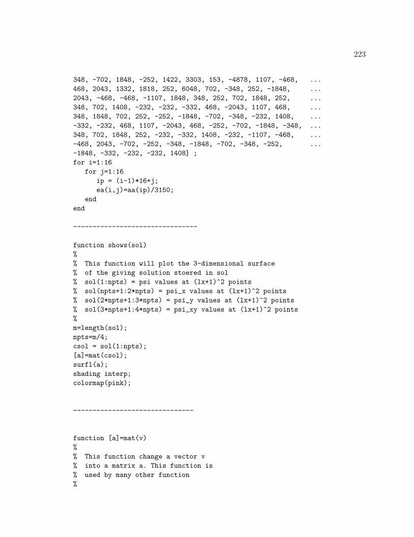
223
348, -702, 1848, -252, 1422, 3303, 153, -4878, 1107, -468, ...468, 2043, 1332, 1818, 252, 6048, 702, -348, 252, -1848, ...2043, -468, -468, -1107, 1848, 348, 252, 702, 1848, 252, ...348, 702, 1408, -232, -232, -332, 468, -2043, 1107, 468, ...348, 1848, 702, 252, -252, -1848, -702, -348, -232, 1408, ...-332, -232, 468, 1107, -2043, 468, -252, -702, -1848, -348, ...348, 702, 1848, 252, -232, -332, 1408, -232, -1107, -468, ...-468, 2043, -702, -252, -348, -1848, -702, -348, -252, ...-1848, -332, -232, -232, 1408] ;for i=1:16
for j=1:16ip = (i-1)*16+j;ea(i,j)=aa(ip)/3150;
endend
--------------------------------
function shows(sol)%% This function will plot the 3-dimensional surface% of the giving solution stoered in sol% sol(1:npts) = psi values at (lx+1)^2 points% sol(npts+1:2*npts) = psi_x values at (lx+1)^2 points% sol(2*npts+1:3*npts) = psi_y values at (lx+1)^2 points% sol(3*npts+1:4*npts) = psi_xy values at (lx+1)^2 points%m=length(sol);npts=m/4;csol = sol(1:npts);[a]=mat(csol);surfl(a);shading interp;colormap(pink);
-------------------------------
function [a]=mat(v)%% This function change a vector v% into a matrix a. This function is% used by many other function%
224
n=length(v);k= sqrt(n) ;for i=1:kfor j=1:km= (i-1)*k + j ;
a(i,j) = v(m) ;end
end
-------------------------------
function [b] = mab%% This function will read the file% bb which contains all values of possible% integral comes from the trilinear term% between the 16 basis functions and store% them in the array b(16,16,16).% b(i,j,k) = b( phi_i ,phi_j ,phi_k)% Note : This function will be Ok only% in MATLAB version 5.0 since the% older version does not support% multi-dimensional array%load bbfor i=1:16
for j=1:16for k=1:16
ip = (i-1)*256 + (j-1)*16 + k;b(i,j,k)=bb(ip)/88200;
endend
end
---------------------------
function [a,rhs] = fboundry(a,rhs,bo,boy)%% In this function, the contributions arrising% from the boundary conditions are added in.%% i.e%
225
% a(:,i)=0 and a(i,:) and a(i,i)=1% for all i in the vector bo and boy%% rhs(i) = 0 for all i in vector bo% rhs(i) = 1 for all i in vector boy%nbo = length(bo);m = length(rhs);lx = sqrt(m/4) - 1;nboy = length(boy);for ii=1:nbo
i=bo(ii);a(i,:)=zeros([1,m]);a(:,i)=zeros([m,1]);a(i,i)=1;rhs(i)=0;
endfor ii=1:nboy
i=boy(ii);a(i,:)=zeros([1,m]);a(:,i)=zeros([m,1]);a(i,i)=1;rhs(i)=1;
end
---------------------------------
function [a,rhs] = boundry(a,rhs,bo,boy)%% In this function, the contributions arising% from the boundry conditions are added in.% i.e% a(i,:)=0 a(:,i) a(i,i)=1% for all i in vectors bo and boy%% rhs(i) = 0 for all i in bo and boy%% in this way no update on the boudry nodes% for all Newton steps.%nbo = length(bo);m = length(rhs);lx = sqrt(m/4) - 1;nboy = length(boy);for ii=1:nbo
226
i=bo(ii);a(i,:)=zeros([1,m]);a(:,i)=zeros([m,1]);a(i,i)=1;rhs(i)=0;
endfor ii=1:nboy
i=boy(ii);a(i,:)=zeros([1,m]);a(:,i)=zeros([m,1]);a(i,i)=1;rhs(i)=0;
end
----------------------------
function [q] = maq%% This function will read the file q1% which contains the values of the 16 basis% functions, the x-derivative , y-derivative% xy-derivative, xx-derivative and yy-derivative% at the integration points and store them in% the array q( 16,6,4).% The first argument of q represents which basis% functions the second argument means which% derivative and the third argument represents% which integration points%% Example :% q(5,3,2) = phi5_y( xi(2) , eta(2) )%load q1for i=1:16for j=1:6for k=1:4
n = (i-1)*24+(j-1)*4+k;q(i,j,k)=q1(n);
endend
end
-------------------------------
function [a] = fstiff(lx,Re,elnode,...

227
xx,yy,lxo,elnodeo,solo,ea,b)%% This function will take the input vector solo% to compute the matrix a in a sparse form.% This a is the matrix coming from step 2% in the algorithm i.e the resulting matrix% needed to solve the linear system in th fine% mesh.% lx = # of squares along x-axis in fine mesh% Re = Renolds number% elnode = global labeling matrix in fine mesh% xx = x-coordinate of all nodes% yy = y-coordinate of all nodes% lxo = # of squares along x-axis in coarse mesh% elnodeo = global labeling matrix in fine mesh% solo = the solution on coarse mesh.% ( output from csolve function )% ea = element stiffnes matrix from maea function% b = element 3-dimenstional matrix from mab function% a = the resulting matrix from step2 i.e resulting% matrix from fine mesh.%nbf = 16;nelem = lx*lx;m = 4*(lx+1)^2;h = 2 / lx;ratio=lx/lxo;%------------assimble stiff ------------a = sparse(m,m);for k=1:nelemfor ix=1:4p= elnode(k,ix);
x(ix) = xx(p);y(ix) = yy(p);endxm=( x(1)+x(2) )/2;ym=( y(1)+y(3) )/2;for ir =1:nbf
i = elnode(k,ir);for is =1:nbfj=elnode(k,is);a(i,j) = a(i,j) + (1/Re)*ea(ir,is)/h^2;
sum = 0;for ik=1:nbfko = findk(xm,ym,lxo);

228
kk=elnodeo(ko,ik);sum=sum + solo(kk)*b(ik,ir,is) ;endsum = sum/(ratio*h^2);a(i,j) = a(i,j) + sum;end
endend
----------------------------------
function k = findk(xm,ym,lx)%% Given a point (xm,yx) in (lx+1)X(lx+1) grid% points the function will return the element% number k such that (xm,ym) inside the k-the% square. This function is needed by many% functions.%h = 2/lx ;x = -1+h ; y = -1+h ;kx =1;ky=1;for i= 2:lx+1if( x > xm )kx = i-1 ;
break ;endx = x + h;
endfor j = 2:lx+1if( y > ym)ky=j -1 ;
break;endy = y + h;
endk = (ky -1)*lx + kx;
-----------------------------
function [x,k] = bicgstab(b,tol,c)%% this function will solve any linear system of% equation with the rhs stored in b and the matrix
229
% are stored in c. this function solves the linear% system c x = b using a bicgstab algorithm.% this algorithm is described in the following% reference:% t. chan j. demmel j. donator j. doncarra v. eijkhout% r. pozo c. romine r. barrett m.berry and h. van dev vorst.% , templates: for the solution of linear systems:% building blocks for iterative methods.% the approximation solution is stored in the vector% x(m) and use this x as the initial guiss. The matrix% is stored in sparse form. k is the number of iteration% needed to reach the required tol.%%k=0;x = zeros([length(b),1]) ;r = c*x ;r = b-r ;rh= r ;for i=1:100
row = rh’*r ;if(row == 0 ) break; end;if(i == 1)
p = r ;else
beta = (row/rowold)*(alpha/w) ;p = r + beta*(p-w*v) ;
endp = p ;v = c*p ;alpha = row/(rh’*v) ;s = r - alpha*v ;if( norm(s)<tol)
k=i ;x=x+alpha*p ;disp(’I stop because norm(s)<tol’);break ;
ends = s ;t = c*s ;w = (t’*s)/(t’*t) ;up = alpha*p +w*s ;x = x + up ;r = s - w*t ;if(w == 0 )

230
disp(’I can not continue iteration because w = 0’);break ;
endif( norm(up)<tol & norm(r)<tol )k = i ;disp(’I stop because norm(r,up)<tol’);break
endrowold=row ;end
-------------------------------------
function [x0] = guiss(lx)%% This function will take the input lx% and returns the vector x0 which is zeros% every where and satisfy the boundry conditions%m=4*(lx+1)^2;[elnode,bo,boy]=maelnode(lx);x0 = zeros([m,1]);x0(boy) = x0(boy) + 1;
-----------------------------------
function [a] = jacobs(lx,Re,sol,elnode,bo,ea,b)%% This function will compute the jacobian matrix of the% problem and store it in the sparse matrix a.% lx = number of squares along x-axis% Re = Reynolds number% sol = i-th iteration from i-th Newton step% elnode = global labeling matrix% bo = boundary nodes% ea = element stiffnes matrix% b = element 3-dimensional array from mab function% a = jacobian matrix at i-th Newton step%nbf = 16;nelem = lx^2;m = 4*(lx+1)^2;h = 2 / lx;%------------assimble Jacobian ------------a = sparse(m,m);
231
for k=1:nelemfor ir =1:nbf
i = elnode(k,ir);for is =1:nbfj=elnode(k,is);a(i,j) = a(i,j) + (1/Re)*ea(ir,is)/h^2;
sum = 0;for ik=1:nbfkk=elnode(k,ik);
brack = b(ir,is,ik) + b(ir,ik,is);sum=sum + sol(kk)*brack/h^2;enda(i,j) = a(i,j) + sum;end
endend
------------------------------------
function [elnode,bo,boy] = maelnode(lx)%% This function computes the element node matrix of% the Bogner-Fox-Schemidt elements and store them in elnode% the boundary points and store them in bo and boy.% Note that the domain is [-1,1]x[-1,1].% lx = # of squares along x-axis% nelem = # of elemnts = lx^2% npts = # of points = (lx+1)^2% h = 2.0 / lx% nbf = # of basis functions in each element = 16% nbo = # of boundary points =% elnode = the global labeling matrix% bo = contains all global boundary numbers except the top% with y-derivative node% boy = contains global boundary numbers on the top with% y-derivative node%% note : the global numbering is going from lower left corner% to the top right corner starting by listing the function% node then x-derivative node then y-derivative node then% xy-derivative node.%npts=(lx+1)^2;m=4*npts;n0 = 0;

232
for i=1:lxfor j= 1:lx
ie = (i-1) * lx + j;k = ie + n0;elnode(ie,1) = k;elnode(ie,2) = k+1;elnode(ie,3) = k+1+lx;elnode(ie,4) = k+2+lx;elnode(ie,5) = k+npts;elnode(ie,6) = k+npts+1;elnode(ie,7) = k+lx+1+npts;elnode(ie,8) = k+lx+2+npts;elnode(ie,9) = k+2*npts;elnode(ie,10) = k+2*npts+1;elnode(ie,11) = k+lx+1+2*npts;elnode(ie,12) = k+lx+2+2*npts;elnode(ie,13) = k+3*npts;elnode(ie,14) = k+1+3*npts;elnode(ie,15) = k+lx+1+3*npts;elnode(ie,16) = k+lx+2+3*npts;
endn0 = n0 + 1;
end% -------------------------------------% Compute boundary node% -------------------------------------for i=1:lx-1
bo(i) = i+1;bo(i+lx-1) = (lx+1)*lx + i + 1;
endfor i=1:lx+1
bo(2*lx-2+i) = (i-1)*(lx + 1) + 1;bo(3*lx-1+i) = i*(lx + 1);
end% -------------------------------------% Compute normal boundary node% -------------------------------------for i=1:4*lxix=i+4*lx;ixy=i+8*lx;bo(ix) = bo(i) + npts;bo(ixy) = bo(i) + 3*npts;
endfor i=1:lx+1
iy=i+12*lx;
233
bo(iy) = i + 2*npts;endfor i=2:lx
iy = i + 13*lx;bo(iy) = i*(lx+1) + 2*npts;
endfor i=2:lx
iy = i - 1 + 14*lx;bo(iy) = (i-1)*(lx+1) + 1;
endfor i=0:lx
boy(i+1)= 3*npts - i;end
--------------------------------
function [x,y] = coord(lx)%% This function will compute the x-coordinate% and y-coordinate of all nodes and store them% in x and y array.% lx = number of square along the x-axis% x = the x-coordinates of all nodes% y = the y-coordinates of all nodes%npts=(lx+1)^2;h = 2/lx;y0 = -1.0d0;for i=1:lx+1
x0 = -1.0d0;for j=1:lx+1
ip = (i-1)*(lx+1) + j;x(ip)= x0;y(ip)= y0;x0 = x0 + h;
endy0 = y0 + h;
endfor i=1:nptsix=i+npts;iy=i+2*npts;ixy=i+3*npts;x(ix) = x(i);x(iy) = x(i);x(ixy) = x(i);
234
y(ix) = y(i);y(iy) = y(i);y(ixy) = y(i);
end
-------------------------------
function [rhs] = force(lx,Re,sol,elnode,bo,xx,yy,ea,b)%% This function will take the input vector sol% to compute F( sol ) and store it in rhs vector% which will be the right hand side of the resulting% linear system from the i-th newton iteration and% in the same time it is the residual.%% lx = # of square along the x-axis% Re = Reynolds number% sol= i-th iteration from Newton method% elnode(nelem,16) = global labeling matrix% bo = boundary nodes% xx = x-coordinates of all nodes% yy = y-coordinates of all nodes% ea = element stiffnes matrix from function maea% b = element 3-dimensional matrix from function% mab% rhs= the rhs vector of the resulting matrix in% the i-th itration before the boundary% condition requirement.%nbf=16;h=2/lx;nelem=lx^2;m=4*(lx+1)^2;rhs = zeros([m,1]) ;for nk=1:nelemfor ii=1:4x(ii) = xx( elnode(nk,ii) ) ;
y(ii) = yy( elnode(nk,ii) ) ;endfor ir=1:nbf
i=elnode(nk,ir) ;sum=0 ;for is=1:nbfj=elnode(nk,is) ;sum = sum + (1/Re)*ea(ir,is)*sol(j);
235
endrhs(i) = rhs(i) + sum/h^2 ;
sum=0 ;for is=1:nbfj=elnode(nk,is) ;for ik=1:nbf
k= elnode(nk,ik) ;sum=sum+b(ir,ik,is)*sol(k)*sol(j) ;
endendrhs(i) = rhs(i) + sum/h^2 ;end
end
----------------------------------
function [xi,eta,w] = squad(n)%% This function will return the integration% points on the square [-1,1]x[-1,1] the% x-coordinates of the points are stored in% array xi and the y-coordinates stored in% array eta and the wight are stored in w%p = 1/sqrt(3);m = -p;xi =[m;p;m;p];eta = [m;m;p;p];w =[1;1;1;1];
-----------------------------------
function backup(i,sol,er)%% This function will save the i-th% solution from Newton step into% a file.%save erorr er -asciiif i == 1save sol1 sol -ascii
elseif i == 2save sol2 sol -ascii
elseif i == 3

236
save sol3 sol -asciielseif i == 4save sol4 sol -ascii
elseif i == 5save sol5 sol -ascii
elseif i == 6save sol6 sol -ascii
elseif i == 7save sol7 sol -ascii
elseif i == 8save sol8 sol -ascii
elseif i == 9save sol9 sol -ascii
elseif i == 10save sol10 sol -ascii
elseif i == 11save sol11 sol -ascii
elseif i == 12save sol12 sol -ascii
elseif i == 13save sol13 sol -ascii
elseif i == 14save sol14 sol -ascii
elseif i == 15save sol15 sol -ascii
elseif i == 16save sol16 sol -ascii
elseif i == 17save sol17 sol -ascii
elseif i == 18save sol18 sol -ascii
elseif i == 19save sol19 sol -ascii
elsesave sol20 sol -ascii
end
---------------------------------
function showc(sol,c)%% This function will plot the streamlines% of the giving solution stoered in sol% sol(1:npts) = psi values at (lx+1)^2 points% sol(npts+1:2*npts) = psi_x values at (lx+1)^2 points
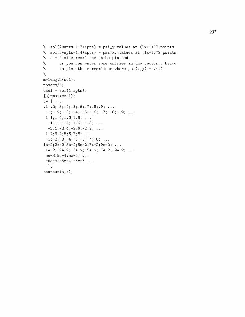
237
% sol(2*npts+1:3*npts) = psi_y values at (lx+1)^2 points% sol(3*npts+1:4*npts) = psi_xy values at (lx+1)^2 points% c = # of streamlines to be plotted% or you can enter some entries in the vector v below% to plot the streamlines where psi(x,y) = v(i).%m=length(sol);npts=m/4;csol = sol(1:npts);[a]=mat(csol);v= [ ....1;.2;.3;.4;.5;.6;.7;.8;.9; ...-.1;-.2;-.3;-.4;-.5;-.6;-.7;-.8;-.9; ...1.1;1.4;1.6;1.8; ...-1.1;-1.4;-1.6;-1.8; ...-2.1;-2.4;-2.6;-2.8; ...1;2;3;4;5;6;7;8; ...-1;-2;-3;-4;-5;-6;-7;-8; ...
1e-2;2e-2;3e-2;5e-2;7e-2;9e-2; ...-1e-2;-2e-2;-3e-2;-5e-2;-7e-2;-9e-2; ...5e-3;5e-4;5e-6; ...-5e-3;-5e-4;-5e-6 ...];
contour(a,c);

Appendix D
Data Files
238
239
This is the content of bb.dat file
0 17010 -17010 0 -3780 -3780
0 0 3780 0 3780 0
0 0 0 0 8505 -25515
8505 8505 378 7182 3402 -3402
-1890 -1890 -1890 -1890 -756 756
-756 756 -8505 -8505 25515 -8505
1890 1890 1890 1890 -378 -3402
-7182 3402 756 756 -756 -756
0 17010 -17010 0 1512 -5292
-5292 1512 -1512 5292 5292 -1512
0 -1512 1512 0 -21615 111
17835 3669 -7935 2505 4155 -1875
7050 1938 -7062 -1590 1830 -960
-1698 804 3291 18213 -7071 -14433
3639 -7935 -3009 4155 -1182 -7806
2346 6306 -708 1830 1056 -1698
2085 -2631 1695 -1149 1635 15
2145 -645 762 -930 -750 582
690 -48 -822 204 -771 1317
4551 -5097 -1119 1635 489 2145
174 -6 -1338 1506 -300 690
-48 -822 21615 -17835 -111 -3669
-7050 7062 -1938 1590 7935 -4155
-2505 1875 -1830 1698 960 -804
-2085 -1695 2631 1149 -762 750
930 -582 -1635 -2145 -15 645
-690 822 48 -204 -3291 7071
-18213 14433 1182 -2346 7806 -6306
-3639 3009 7935 -4155 708 -1056
-1830 1698 771 -4551 -1317 5097
-174 1338 6 -1506 1119 -489
-1635 -2145 300 48 -690 822
0 -6762 6762 0 -810 2238
1272 -180 810 -1272 -2238 180
0 402 -402 0 462 6300
-2520 -4242 138 -810 -1020 1272
264 198 576 1482 66 0
252 -402 -462 2520 -6300 4242
-264 -576 -198 -1482 -138 1020
810 -1272 -66 -252 0 402
0 -2058 2058 0 264 -264
240
618 -198 -264 -618 264 198
0 -66 66 0 25515 -8505
-8505 -8505 7182 378 -3402 3402
1890 1890 1890 1890 756 -756
756 -756 -17010 0 0 17010
-3780 -3780 0 0 0 -3780
0 -3780 0 0 0 0
-17010 0 0 17010 -5292 1512
1512 -5292 -5292 1512 1512 -5292
-1512 0 0 1512 8505 8505
8505 -25515 1890 1890 1890 1890
3402 378 -3402 7182 756 756
-756 -756 18213 3291 -14433 -7071
7935 -3639 -4155 3009 -7806 -1182
6306 2346 -1830 708 1698 -1056
111 -21615 3669 17835 -2505 7935
1875 -4155 1938 7050 -1590 -7062
960 -1830 -804 1698 1317 -771
-5097 4551 -1635 1119 -2145 -489
-6 174 1506 -1338 -690 300
822 48 -2631 2085 -1149 1695
-15 -1635 645 -2145 -930 762
582 -750 48 -690 -204 822
1695 2085 -1149 -2631 750 -762
-582 930 2145 1635 -645 15
822 -690 -204 48 17835 -21615
3669 111 7062 -7050 1590 -1938
4155 -7935 -1875 2505 1698 -1830
-804 960 4551 -771 -5097 1317
1338 -174 -1506 6 489 -1119
2145 1635 48 300 822 -690
-7071 3291 -14433 18213 -2346 1182
-6306 7806 -3009 3639 4155 -7935
-1056 708 1698 -1830 6300 462
-4242 -2520 810 -138 -1272 1020
198 264 1482 576 0 -66
402 -252 -6762 0 0 6762
-2238 810 180 -1272 -1272 810
180 -2238 -402 0 0 402
-2058 0 0 2058 264 -264
198 -618 -618 -264 198 264
66 0 0 -66 2520 -462

241
4242 -6300 576 264 1482 198
1020 -138 -1272 810 252 66
-402 0 -25515 8505 8505 8505
-1890 -1890 -1890 -1890 -7182 3402
-378 -3402 -756 -756 756 756
17010 0 0 -17010 5292 -1512
-1512 5292 5292 -1512 -1512 5292
1512 0 0 -1512 17010 0
0 -17010 0 0 3780 3780
3780 0 3780 0 0 0
0 0 -8505 -8505 -8505 25515
-3402 3402 -378 -7182 -1890 -1890
-1890 -1890 -756 756 -756 756
-1695 1149 -2085 2631 -2145 645
-1635 -15 -750 582 762 -930
-822 204 690 -48 -4551 5097
771 -1317 -489 -2145 1119 -1635
-1338 1506 174 -6 -48 -822
-300 690 -17835 -3669 21615 -111
-4155 1875 7935 -2505 -7062 -1590
7050 1938 -1698 804 1830 -960
7071 14433 -3291 -18213 3009 -4155
-3639 7935 2346 6306 -1182 -7806
1056 -1698 -708 1830 -18213 14433
-3291 7071 7806 -6306 1182 -2346
-7935 4155 3639 -3009 1830 -1698
-708 1056 -1317 5097 771 -4551
6 -1506 -174 1338 1635 2145
-1119 489 690 -822 -300 -48
-111 -3669 21615 -17835 -1938 1590
-7050 7062 2505 -1875 -7935 4155
-960 804 1830 -1698 2631 1149
-2085 -1695 930 -582 -762 750
15 -645 1635 2145 -48 204
690 -822 -6300 4242 -462 2520
-198 -1482 -264 -576 -810 1272
138 -1020 0 -402 66 252
2058 0 0 -2058 618 -198
264 -264 -264 -198 264 618
-66 0 0 66 6762 0
0 -6762 1272 -180 -810 2238
2238 -180 -810 1272 402 0
242
0 -402 -2520 -4242 462 6300
-1020 1272 138 -810 -576 -1482
-264 -198 -252 402 -66 0
0 -17010 17010 0 -1512 5292
5292 -1512 1512 -5292 -5292 1512
0 1512 -1512 0 -8505 25515
-8505 -8505 -1890 -1890 -1890 -1890
-3402 7182 3402 378 -756 -756
756 756 8505 8505 -25515 8505
3402 -3402 -7182 -378 1890 1890
1890 1890 756 -756 756 -756
0 -17010 17010 0 0 0
3780 3780 0 -3780 0 -3780
0 0 0 0 5097 -4551
-1317 771 2145 489 1635 -1119
1506 -1338 -6 174 822 48
-690 300 1149 -1695 2631 -2085
-645 2145 15 1635 582 -750
-930 762 -204 822 48 -690
14433 7071 -18213 -3291 4155 -3009
-7935 3639 6306 2346 -7806 -1182
1698 -1056 -1830 708 -3669 -17835
-111 21615 -1875 4155 2505 -7935
-1590 -7062 1938 7050 -804 1698
960 -1830 -5097 1317 4551 -771
-1506 6 1338 -174 -2145 -1635
-489 1119 -822 690 -48 -300
-14433 18213 -7071 3291 -6306 7806
-2346 1182 -4155 7935 3009 -3639
-1698 1830 1056 -708 -1149 -2631
1695 2085 -582 930 750 -762
645 -15 -2145 -1635 204 -48
-822 690 3669 111 17835 -21615
1590 -1938 7062 -7050 1875 -2505
-4155 7935 804 -960 -1698 1830
0 2058 -2058 0 198 -618
264 -264 -198 -264 618 264
0 66 -66 0 4242 -6300
2520 -462 1482 198 576 264
1272 -810 -1020 138 402 0
-252 -66 -4242 -2520 6300 462
-1272 1020 810 -138 -1482 -576

243
-198 -264 -402 252 0 66
0 6762 -6762 0 180 -1272
-2238 810 -180 2238 1272 -810
0 -402 402 0 14055 7449
-17835 -3669 375 -1245 -4155 1875
-7050 -1938 7062 1590 -1830 960
1698 -804 -10653 -10851 14433 7071
-375 2379 4155 -3009 7806 1182
-6306 -2346 1830 -708 -1698 1056
1695 -1149 2085 -2631 2145 -645
1635 15 750 -582 -762 930
822 -204 -690 48 -5097 4551
1317 -771 -2145 -489 -1635 1119
-1506 1338 6 -174 -822 -48
690 -300 10920 3780 -14700 0
5040 -840 0 0 -10500 0
7140 0 0 0 0 0
9114 7854 -8484 -8484 1606 -3286
-2446 2446 -4998 -4998 3822 3822
-1292 1292 1060 -1060 9240 -1890
-5460 -1890 -2520 420 -2520 420
2436 -756 924 756 -1008 168
1008 -168 2226 2856 -2856 -2226
914 -74 -74 914 462 714
714 462 284 52 -52 -284
11100 -4338 -4338 -2424 1830 1008
-1368 1050 1830 -1368 1008 1050
120 432 432 -432 -3288 -3474
5346 1416 -1830 1596 1368 -714
690 -1152 -2016 -42 -120 408
-432 96 -3474 1416 -3288 5346
-1152 -42 690 -2016 -1596 714
1830 -1368 -408 -96 120 432
2466 -408 -4524 2466 1152 -294
-690 -588 588 294 690 -1152
408 -240 -120 408 8280 -3030
-4668 -582 -1800 972 -216 204
-360 -690 2010 300 -360 228
120 -104 1308 4446 -3240 -2514
772 -844 -856 760 -654 108
1296 930 -56 8 312 -268
-4908 1338 1296 2274 1224 -372

244
792 -804 -1182 552 -360 -690
456 -160 -360 228 -1044 -2022
2976 90 -488 248 572 -164
-132 -582 -654 108 -136 68
-56 8 -10851 -10653 7071 14433
-2379 375 3009 -4155 1182 7806
-2346 -6306 708 -1830 -1056 1698
7449 14055 -3669 -17835 1245 -375
-1875 4155 -1938 -7050 1590 7062
-960 1830 804 -1698 4551 -5097
-771 1317 489 2145 -1119 1635
1338 -1506 -174 6 48 822
300 -690 -1149 1695 -2631 2085
645 -2145 -15 -1635 -582 750
930 -762 204 -822 -48 690
-7854 -9114 8484 8484 -3286 1606
2446 -2446 4998 4998 -3822 -3822
1292 -1292 -1060 1060 -3780 -10920
0 14700 -840 5040 0 0
0 10500 0 -7140 0 0
0 0 -2856 -2226 2226 2856
-74 914 914 -74 -714 -462
-462 -714 52 284 -284 -52
1890 -9240 1890 5460 420 -2520
420 -2520 756 -2436 -756 -924
168 -1008 -168 1008 -3474 -3288
1416 5346 -1596 1830 714 -1368
-1152 690 -42 -2016 -408 120
-96 432 -4338 11100 -2424 -4338
-1008 -1830 -1050 1368 -1368 1830
1050 1008 -432 -120 432 -432
-408 2466 2466 -4524 294 -1152
588 690 294 588 -1152 690
240 -408 -408 120 1416 -3474
5346 -3288 42 1152 2016 -690
714 -1596 -1368 1830 96 408
-432 -120 -4446 -1308 2514 3240
-844 772 760 -856 -108 654
-930 -1296 8 -56 -268 312
3030 -8280 582 4668 972 -1800
204 -216 690 360 -300 -2010
228 -360 -104 120 2022 1044

245
-90 -2976 248 -488 -164 572
582 132 -108 654 68 -136
8 -56 -1338 4908 -2274 -1296
-372 1224 -804 792 -552 1182
690 360 -160 456 228 -360
-2085 2631 -1695 1149 -1635 -15
-2145 645 -762 930 750 -582
-690 48 822 -204 -1317 771
5097 -4551 1635 -1119 2145 489
6 -174 -1506 1338 690 -300
-822 -48 17835 3669 -14055 -7449
4155 -1875 -375 1245 7062 1590
-7050 -1938 1698 -804 -1830 960
-14433 -7071 10653 10851 -4155 3009
375 -2379 -6306 -2346 7806 1182
-1698 1056 1830 -708 5460 1890
-9240 1890 2520 -420 2520 -420
924 756 2436 -756 1008 -168
-1008 168 2856 2226 -2226 -2856
74 -914 -914 74 714 462
462 714 -52 -284 284 52
14700 0 -10920 -3780 0 0
-5040 840 7140 0 -10500 0
0 0 0 0 8484 8484
-9114 -7854 2446 -2446 -1606 3286
3822 3822 -4998 -4998 1060 -1060
-1292 1292 -3288 5346 -3474 1416
690 -2016 -1152 -42 -1830 1368
1596 -714 -120 -432 408 96
-4524 2466 2466 -408 -690 -588
1152 -294 -690 1152 -588 -294
120 -408 -408 240 -4338 -2424
11100 -4338 -1368 1050 1830 1008
-1008 -1050 -1830 1368 -432 432
-120 -432 5346 1416 -3288 -3474
1368 -714 -1830 1596 2016 42
-690 1152 432 -96 120 -408
1296 2274 -4908 1338 792 -804
1224 -372 360 690 1182 -552
360 -228 -456 160 2976 90
-1044 -2022 572 -164 -488 248
654 -108 132 582 56 -8
246
136 -68 -4668 -582 8280 -3030
-216 204 -1800 972 -2010 -300
360 690 -120 104 360 -228
-3240 -2514 1308 4446 -856 760
772 -844 -1296 -930 654 -108
-312 268 56 -8 771 -1317
-4551 5097 1119 -1635 -489 -2145
-174 6 1338 -1506 300 -690
48 822 2631 -2085 1149 -1695
15 1635 -645 2145 930 -762
-582 750 -48 690 204 -822
-7071 -14433 10851 10653 -3009 4155
2379 -375 -2346 -6306 1182 7806
-1056 1698 708 -1830 3669 17835
-7449 -14055 1875 -4155 -1245 375
1590 7062 -1938 -7050 804 -1698
-960 1830 -2226 -2856 2856 2226
-914 74 74 -914 -462 -714
-714 -462 -284 -52 52 284
-1890 -5460 -1890 9240 -420 2520
-420 2520 -756 -924 756 -2436
-168 1008 168 -1008 -8484 -8484
7854 9114 -2446 2446 3286 -1606
-3822 -3822 4998 4998 -1060 1060
1292 -1292 0 -14700 3780 10920
0 0 840 -5040 0 -7140
0 10500 0 0 0 0
2466 -4524 -408 2466 588 690
294 -1152 1152 -690 -294 -588
408 -120 -240 408 5346 -3288
1416 -3474 2016 -690 42 1152
1368 -1830 -714 1596 432 120
-96 -408 1416 5346 -3474 -3288
714 -1368 -1596 1830 42 2016
1152 -690 96 -432 408 -120
-2424 -4338 -4338 11100 -1050 1368
-1008 -1830 -1050 -1008 1368 -1830
-432 432 432 120 -90 -2976
2022 1044 -164 572 248 -488
108 -654 -582 -132 -8 56
-68 136 -2274 -1296 -1338 4908
-804 792 -372 1224 -690 -360

247
552 -1182 -228 360 160 -456
2514 3240 -4446 -1308 760 -856
-844 772 930 1296 108 -654
268 -312 -8 56 582 4668
3030 -8280 204 -216 972 -1800
300 2010 -690 -360 104 -120
-228 360 -14055 17835 -7449 3669
7050 -7062 1938 -1590 -375 4155
1245 -1875 1830 -1698 -960 804
-1695 -2085 1149 2631 -750 762
582 -930 -2145 -1635 645 -15
-822 690 204 -48 10653 -14433
10851 -7071 -7806 6306 -1182 2346
375 -4155 -2379 3009 -1830 1698
708 -1056 5097 -1317 -4551 771
1506 -6 -1338 174 2145 1635
489 -1119 822 -690 48 300
-11100 4338 4338 2424 -1830 -1008
1368 -1050 -1830 1368 -1008 -1050
-120 -432 -432 432 3474 3288
-1416 -5346 1596 -1830 -714 1368
1152 -690 42 2016 408 -120
96 -432 3288 -5346 3474 -1416
-690 2016 1152 42 1830 -1368
-1596 714 120 432 -408 -96
-2466 4524 408 -2466 -588 -690
-294 1152 -1152 690 294 588
-408 120 240 -408 -10920 14700
-3780 0 10500 -7140 0 0
-5040 0 840 0 0 0
0 0 -9240 5460 1890 1890
-2436 -924 756 -756 2520 2520
-420 -420 1008 -1008 -168 168
-9114 8484 -7854 8484 4998 -3822
4998 -3822 -1606 2446 3286 -2446
1292 -1060 -1292 1060 -2226 2856
-2856 2226 -462 -714 -714 -462
-914 74 74 -914 -284 52
-52 284 -8280 4668 3030 582
360 -2010 690 -300 1800 216
-972 -204 360 -120 -228 104
4908 -1296 -1338 -2274 1182 360
248
-552 690 -1224 -792 372 804
-456 360 160 -228 -1308 3240
-4446 2514 654 -1296 -108 -930
-772 856 844 -760 56 -312
-8 268 1044 -2976 2022 -90
132 654 582 -108 488 -572
-248 164 136 56 -68 -8
2085 1695 -2631 -1149 762 -750
-930 582 1635 2145 15 -645
690 -822 -48 204 -17835 14055
-3669 7449 -7062 7050 -1590 1938
-4155 375 1875 -1245 -1698 1830
804 -960 1317 -5097 -771 4551
-6 1506 174 -1338 -1635 -2145
1119 -489 -690 822 300 48
14433 -10653 7071 -10851 6306 -7806
2346 -1182 4155 -375 -3009 2379
1698 -1830 -1056 708 3288 3474
-5346 -1416 1830 -1596 -1368 714
-690 1152 2016 42 120 -408
432 -96 4338 -11100 2424 4338
1008 1830 1050 -1368 1368 -1830
-1050 -1008 432 120 -432 432
4524 -2466 -2466 408 690 588
-1152 294 690 -1152 588 294
-120 408 408 -240 -5346 3288
-1416 3474 -2016 690 -42 -1152
-1368 1830 714 -1596 -432 -120
96 408 -5460 9240 -1890 -1890
-924 -2436 -756 756 -2520 -2520
420 420 -1008 1008 168 -168
-14700 10920 0 3780 -7140 10500
0 0 0 5040 0 -840
0 0 0 0 -2856 2226
-2226 2856 -714 -462 -462 -714
-74 914 914 -74 52 -284
284 -52 -8484 9114 -8484 7854
-3822 4998 -3822 4998 -2446 1606
2446 -3286 -1060 1292 1060 -1292
-1296 4908 -2274 -1338 -360 -1182
-690 552 -792 -1224 804 372
-360 456 228 -160 4668 -8280
249
582 3030 2010 -360 300 -690
216 1800 -204 -972 120 -360
-104 228 -2976 1044 -90 2022
-654 -132 108 -582 -572 488
164 -248 -56 -136 8 68
3240 -1308 2514 -4446 1296 -654
930 108 856 -772 -760 844
312 -56 -268 8 10851 -7071
10653 -14433 -1182 2346 -7806 6306
2379 -3009 -375 4155 -708 1056
1830 -1698 -4551 771 5097 -1317
-1338 174 1506 -6 -489 1119
-2145 -1635 -48 -300 -822 690
-7449 3669 -14055 17835 1938 -1590
7050 -7062 -1245 1875 375 -4155
960 -804 -1830 1698 1149 2631
-1695 -2085 582 -930 -750 762
-645 15 2145 1635 -204 48
822 -690 3474 -1416 3288 -5346
1152 42 -690 2016 1596 -714
-1830 1368 408 96 -120 -432
408 -2466 -2466 4524 -294 1152
-588 -690 -294 -588 1152 -690
-240 408 408 -120 4338 2424
-11100 4338 1368 -1050 -1830 -1008
1008 1050 1830 -1368 432 -432
120 432 -1416 -5346 3474 3288
-714 1368 1596 -1830 -42 -2016
-1152 690 -96 432 -408 120
7854 -8484 9114 -8484 -4998 3822
-4998 3822 3286 -2446 -1606 2446
-1292 1060 1292 -1060 2856 -2226
2226 -2856 714 462 462 714
74 -914 -914 74 -52 284
-284 52 3780 0 10920 -14700
0 0 -10500 7140 840 0
-5040 0 0 0 0 0
-1890 -1890 9240 -5460 -756 756
2436 924 -420 -420 2520 2520
-168 168 1008 -1008 4446 -2514
1308 -3240 108 930 -654 1296
844 -760 -772 856 -8 268

250
56 -312 -2022 90 -1044 2976
-582 108 -132 -654 -248 164
488 -572 -68 -8 136 56
-3030 -582 8280 -4668 -690 300
-360 2010 -972 -204 1800 216
-228 104 360 -120 1338 2274
-4908 1296 552 -690 -1182 -360
372 804 -1224 -792 160 -228
-456 360 -771 4551 1317 -5097
174 -1338 -6 1506 -1119 489
1635 2145 -300 -48 690 -822
7071 -10851 14433 -10653 2346 -1182
6306 -7806 3009 -2379 -4155 375
1056 -708 -1698 1830 -2631 -1149
2085 1695 -930 582 762 -750
-15 645 -1635 -2145 48 -204
-690 822 -3669 7449 -17835 14055
-1590 1938 -7062 7050 -1875 1245
4155 -375 -804 960 1698 -1830
-2466 408 4524 -2466 -1152 294
690 588 -588 -294 -690 1152
-408 240 120 -408 -1416 3474
-5346 3288 -42 -1152 -2016 690
-714 1596 1368 -1830 -96 -408
432 120 -5346 -1416 3288 3474
-1368 714 1830 -1596 -2016 -42
690 -1152 -432 96 -120 408
2424 4338 4338 -11100 1050 -1368
1008 1830 1050 1008 -1368 1830
432 -432 -432 -120 2226 -2856
2856 -2226 462 714 714 462
914 -74 -74 914 284 -52
52 -284 8484 -7854 8484 -9114
3822 -4998 3822 -4998 2446 -3286
-2446 1606 1060 -1292 -1060 1292
1890 1890 5460 -9240 756 -756
924 2436 420 420 -2520 -2520
168 -168 -1008 1008 0 -3780
14700 -10920 0 0 7140 -10500
0 -840 0 5040 0 0
0 0 90 -2022 2976 -1044
-108 582 654 132 164 -248

251
-572 488 8 68 -56 -136
-2514 4446 -3240 1308 -930 -108
-1296 654 -760 844 856 -772
-268 8 312 -56 2274 1338
1296 -4908 690 -552 360 1182
804 372 -792 -1224 228 -160
-360 456 -582 -3030 -4668 8280
-300 690 -2010 360 -204 -972
216 1800 -104 228 120 -360
0 6762 -6762 0 810 -2238
-1272 180 -810 1272 2238 -180
0 -402 402 0 -6300 -462
4242 2520 -810 138 1272 -1020
-198 -264 -1482 -576 0 66
-402 252 6300 -4242 462 -2520
198 1482 264 576 810 -1272
-138 1020 0 402 -66 -252
0 -2058 2058 0 -198 618
-264 264 198 264 -618 -264
0 -66 66 0 2220 3030
-5832 582 1800 -972 216 -204
-1740 690 2610 -300 360 -228
-120 104 4446 1308 -2514 -3240
844 -772 -760 856 108 -654
930 1296 -8 56 268 -312
5844 -2274 -2232 -1338 -792 804
-1224 372 1740 -690 78 552
-360 228 456 -160 90 2976
-2022 -1044 164 -572 -248 488
-108 654 582 132 8 -56
68 -136 -2220 5832 -3030 -582
1740 -2610 -690 300 -1800 -216
972 204 -360 120 228 -104
-5844 2232 2274 1338 -1740 -78
690 -552 792 1224 -804 -372
360 -456 -228 160 -4446 2514
-1308 3240 -108 -930 654 -1296
-844 760 772 -856 8 -268
-56 312 -90 2022 -2976 1044
108 -582 -654 -132 -164 248
572 -488 -8 -68 56 136
0 2100 -2100 0 0 -840
252
0 0 0 0 840 0
0 0 0 0 2982 -378
-1302 -1302 808 32 -388 388
-336 -336 476 476 -144 144
136 -136 -2982 1302 378 1302
336 -476 336 -476 -808 388
-32 -388 144 -136 -144 136
0 -1764 1764 0 -88 396
396 -88 88 -396 -396 88
0 64 -64 0 -462 -6300
2520 4242 -138 810 1020 -1272
-264 -198 -576 -1482 -66 0
-252 402 6762 0 0 -6762
2238 -810 -180 1272 1272 -810
-180 2238 402 0 0 -402
-2058 0 0 2058 -618 198
-264 264 264 198 -264 -618
66 0 0 -66 -4242 6300
-2520 462 -1482 -198 -576 -264
-1272 810 1020 -138 -402 0
252 66 -1308 -4446 3240 2514
-772 844 856 -760 654 -108
-1296 -930 56 -8 -312 268
-3030 -2220 -582 5832 -972 1800
-204 216 -690 1740 300 -2610
-228 360 104 -120 -2976 -90
1044 2022 -572 164 488 -248
-654 108 -132 -582 -56 8
-136 68 2274 -5844 1338 2232
804 -792 372 -1224 690 -1740
-552 -78 228 -360 -160 456
2232 -5844 1338 2274 78 1740
552 -690 1224 792 -372 -804
456 -360 -160 228 5832 -2220
-582 -3030 2610 -1740 -300 690
-216 -1800 204 972 -120 360
104 -228 2022 -90 1044 -2976
582 -108 132 654 248 -164
-488 572 68 8 -136 -56
2514 -4446 3240 -1308 930 108
1296 -654 760 -844 -856 772
268 -8 -312 56 378 -2982
253
1302 1302 32 808 388 -388
336 336 -476 -476 144 -144
-136 136 -2100 0 0 2100
-840 0 0 0 0 0
0 -840 0 0 0 0
1764 0 0 -1764 396 -88
-88 396 396 -88 -88 396
64 0 0 -64 -1302 2982
-1302 -378 -476 336 -476 336
-388 808 388 32 -136 144
136 -144 462 -2520 6300 -4242
264 576 198 1482 138 -1020
-810 1272 66 252 0 -402
2058 0 0 -2058 -264 264
-198 618 618 264 -198 -264
-66 0 0 66 -6762 0
0 6762 -1272 180 810 -2238
-2238 180 810 -1272 -402 0
0 402 4242 2520 -6300 -462
1272 -1020 -810 138 1482 576
198 264 402 -252 0 -66
-2232 -1338 5844 -2274 -1224 372
-792 804 -78 -552 -1740 690
-456 160 360 -228 -2022 -1044
90 2976 -248 488 164 -572
-582 -132 108 -654 -68 136
-8 56 -5832 582 2220 3030
216 -204 1800 -972 -2610 300
1740 -690 120 -104 -360 228
-2514 -3240 4446 1308 -760 856
844 -772 -930 -1296 -108 654
-268 312 8 -56 1308 -3240
4446 -2514 -654 1296 108 930
772 -856 -844 760 -56 312
8 -268 2976 -1044 90 -2022
654 132 -108 582 572 -488
-164 248 56 136 -8 -68
3030 582 2220 -5832 690 -300
-1740 2610 972 204 -1800 -216
228 -104 -360 120 -2274 -1338
5844 -2232 -690 552 1740 78
-804 -372 792 1224 -228 160
254
360 -456 -378 -1302 2982 -1302
-336 476 -336 476 -32 -388
-808 388 -144 136 144 -136
-1764 0 0 1764 -396 88
88 -396 -396 88 88 -396
-64 0 0 64 2100 0
0 -2100 0 0 0 840
840 0 0 0 0 0
0 0 1302 1302 -2982 378
388 -388 -808 -32 476 476
-336 -336 136 -136 -144 144
0 2058 -2058 0 -264 264
-618 198 264 618 -264 -198
0 66 -66 0 -2520 462
-4242 6300 -576 -264 -1482 -198
-1020 138 1272 -810 -252 -66
402 0 2520 4242 -462 -6300
1020 -1272 -138 810 576 1482
264 198 252 -402 66 0
0 -6762 6762 0 -180 1272
2238 -810 180 -2238 -1272 810
0 402 -402 0 1044 2022
-2976 -90 488 -248 -572 164
132 582 654 -108 136 -68
56 -8 1338 2232 2274 -5844
372 -1224 804 -792 552 78
-690 1740 160 -456 -228 360
3240 2514 -1308 -4446 856 -760
-772 844 1296 930 -654 108
312 -268 -56 8 -582 5832
-3030 -2220 -204 216 -972 1800
-300 2610 690 -1740 -104 120
228 -360 -1044 2976 -2022 90
-132 -654 -582 108 -488 572
248 -164 -136 -56 68 8
-3240 1308 -2514 4446 -1296 654
-930 -108 -856 772 760 -844
-312 56 268 -8 -1338 -2274
-2232 5844 -552 690 -78 -1740
-372 -804 1224 792 -160 228
456 -360 582 3030 -5832 2220
300 -690 -2610 1740 204 972
255
-216 -1800 104 -228 -120 360
0 1764 -1764 0 88 -396
-396 88 -88 396 396 -88
0 -64 64 0 1302 378
1302 -2982 476 -336 476 -336
388 32 -388 808 136 -144
-136 144 -1302 -1302 -378 2982
-388 388 -32 -808 -476 -476
336 336 -136 136 144 -144
0 -2100 2100 0 0 0
840 0 0 -840 0 0
0 0 0 0

256
This is the content of ea.dat file
9288 -4563 -4563 -162 4878 3303
-153 1422 4878 -153 3303 1422
2043 468 468 -1107 -4563 9288
-162 -4563 -3303 -4878 -1422 153
-153 4878 1422 3303 -468 -2043
1107 -468 -4563 -162 9288 -4563
-153 1422 4878 3303 -3303 -1422
-4878 153 -468 1107 -2043 -468
-162 -4563 -4563 9288 -1422 153
-3303 -4878 -1422 -3303 153 -4878
-1107 468 468 2043 4878 -3303
-153 -1422 6048 1818 252 1332
2043 -468 468 1107 1848 348
-252 -702 3303 -4878 1422 153
1818 6048 1332 252 468 -2043
-1107 -468 348 1848 -702 -252
-153 -1422 4878 -3303 252 1332
6048 1818 -468 -1107 -2043 468
252 702 -1848 -348 1422 153
3303 -4878 1332 252 1818 6048
1107 468 -468 2043 702 252
-348 -1848 4878 -153 -3303 -1422
2043 468 -468 1107 6048 252
1818 1332 1848 -252 348 -702
-153 4878 -1422 -3303 -468 -2043
-1107 468 252 6048 1332 1818
252 -1848 702 -348 3303 1422
-4878 153 468 -1107 -2043 -468
1818 1332 6048 252 348 -702
1848 -252 1422 3303 153 -4878
1107 -468 468 2043 1332 1818
252 6048 702 -348 252 -1848
2043 -468 -468 -1107 1848 348
252 702 1848 252 348 702
1408 -232 -232 -332 468 -2043
1107 468 348 1848 702 252
-252 -1848 -702 -348 -232 1408
-332 -232 468 1107 -2043 468
-252 -702 -1848 -348 348 702
1848 252 -232 -332 1408 -232
-1107 -468 -468 2043 -702 -252
257
-348 -1848 -702 -348 -252 -1848
-332 -232 -232 1408
258
This is the content of q1.dat file
.783048327607898600 .101851851851851800 .101851851851851800
.013247968688397720 -.442450089729875100 -.442450089729875100
-.057549910270124770 -.057549910270124770 -.442450089729875100
-.057549910270124770 -.442450089729875100 -.057549910270124770
-.766346035225552500 .766346035225552500 -.099679368558885910
.099679368558885910 -.766346035225552500 -.099679368558885910
.766346035225552500 .099679368558885910 .250000000000000000
.250000000000000000 .250000000000000000 .250000000000000000
.101851851851851800 .783048327607898600 .013247968688397720
.101851851851851800 .442450089729875100 .442450089729875100
.057549910270124770 .057549910270124770 -.057549910270124770
-.442450089729875100 -.057549910270124770 -.442450089729875100
.766346035225552500 -.766346035225552500 .099679368558885910
-.099679368558885910 -.099679368558885910 -.766346035225552500
.099679368558885910 .766346035225552500 -.250000000000000000
-.250000000000000000 -.250000000000000000 -.250000000000000000
.101851851851851800 .013247968688397720 .783048327607898600
.101851851851851800 -.057549910270124770 -.057549910270124770
-.442450089729875100 -.442450089729875100 .442450089729875100
.057549910270124770 .442450089729875100 .057549910270124770
-.099679368558885910 .099679368558885910 -.766346035225552500
.766346035225552500 .766346035225552500 .099679368558885910
-.766346035225552500 -.099679368558885910 -.250000000000000000
-.250000000000000000 -.250000000000000000 -.250000000000000000
.013247968688397720 .101851851851851800 .101851851851851800
.783048327607898600 .057549910270124770 .057549910270124770
.442450089729875100 .442450089729875100 .057549910270124770
.442450089729875100 .057549910270124770 .442450089729875100
.099679368558885910 -.099679368558885910 .766346035225552500
-.766346035225552500 .099679368558885910 .766346035225552500
-.099679368558885910 -.766346035225552500 .250000000000000000
.250000000000000000 .250000000000000000 .250000000000000000
.232632922712797500 .062333803773785870 .030258788818806710
.008107818027943149 .255448678408517600 -.255448678408517600
.033226456186295350 -.033226456186295350 -.131445855765802100
-.035220810900864550 -.131445855765802100 -.035220810900864550
1.208796124955427000 .323895945495677300 -.157229278829010600
.042129458288761130 -.227670900630739700 -.061004233964073060
.227670900630739700 .061004233964073060 -.144337567297406300
.144337567297406300 -.144337567297406300 .144337567297406300
-.062333803773785870 -.232632922712797500 -.008107818027943149

259
-.030258788818806710 -.255448678408517600 .255448678408517600
-.033226456186295350 .033226456186295350 .035220810900864550
.131445855765802100 .035220810900864550 .131445855765802100
-.323895945495677300 1.208796124955427000 -.042129458288761130
.157229278829010600 .061004233964073060 .227670900630739700
-.061004233964073060 -.227670900630739700 .144337567297406300
-.144337567297406300 .144337567297406300 -.144337567297406300
.030258788818806710 .008107818027943149 .232632922712797500
.062333803773785870 .033226456186295350 -.033226456186295350
.255448678408517600 -.255448678408517600 .131445855765802100
.035220810900864550 .131445855765802100 .035220810900864550
-.157229278829010600 .042129458288761130 -1.208796124955427000
.323895945495677300 .227670900630739700 .061004233964073060
-.227670900630739700 -.061004233964073060 .144337567297406300
-.144337567297406300 .144337567297406300 -.144337567297406300
-.008107818027943149 -.030258788818806710 -.062333803773785870
-.232632922712797500 -.033226456186295350 .033226456186295350
-.255448678408517600 .255448678408517600 -.035220810900864550
-.131445855765802100 -.035220810900864550 -.131445855765802100
-.042129458288761130 .157229278829010600 -.323895945495677300
1.208796124955427000 -.061004233964073060 -.227670900630739700
.061004233964073060 .227670900630739700 -.144337567297406300
.144337567297406300 -.144337567297406300 .144337567297406300
.232632922712797500 .030258788818806710 .062333803773785870
.008107818027943149 -.131445855765802100 -.131445855765802100
-.035220810900864550 -.035220810900864550 .255448678408517600
.033226456186295350 -.255448678408517600 -.033226456186295350
-.227670900630739700 .227670900630739700 -.061004233964073060
.061004233964073060 -1.208796124955427000 -.157229278829010600
.323895945495677300 .042129458288761130 -.144337567297406300
-.144337567297406300 .144337567297406300 .144337567297406300
.030258788818806710 .232632922712797500 .008107818027943149
.062333803773785870 .131445855765802100 .131445855765802100
.035220810900864550 .035220810900864550 .033226456186295350
.255448678408517600 -.033226456186295350 -.255448678408517600
.227670900630739700 -.227670900630739700 .061004233964073060
-.061004233964073060 -.157229278829010600 -1.208796124955427000
.042129458288761130 .323895945495677300 .144337567297406300
.144337567297406300 -.144337567297406300 -.144337567297406300
-.062333803773785870 -.008107818027943149 -.232632922712797500
-.030258788818806710 .035220810900864550 .035220810900864550
.131445855765802100 .131445855765802100 -.255448678408517600

260
-.033226456186295350 .255448678408517600 .033226456186295350
.061004233964073060 -.061004233964073060 .227670900630739700
-.227670900630739700 -.323895945495677300 -.042129458288761130
1.208796124955427000 .157229278829010600 .144337567297406300
.144337567297406300 -.144337567297406300 -.144337567297406300
-.008107818027943149 -.062333803773785870 -.030258788818806710
-.232632922712797500 -.035220810900864550 -.035220810900864550
-.131445855765802100 -.131445855765802100 -.033226456186295350
-.255448678408517600 .033226456186295350 .255448678408517600
-.061004233964073060 .061004233964073060 -.227670900630739700
.227670900630739700 -.042129458288761130 -.323895945495677300
.157229278829010600 1.208796124955427000 -.144337567297406300
-.144337567297406300 .144337567297406300 .144337567297406300
.069112051992016260 .018518518518518510 .018518518518518510
.004962022082057822 .075890300210246580 -.075890300210246580
.020334744654691040 -.020334744654691040 .075890300210246580
.020334744654691040 -.075890300210246580 -.020334744654691040
-.359116756396541800 .096225044864937560 -.096225044864937560
.025783423063208550 -.359116756396541800 -.096225044864937560
.096225044864937560 .025783423063208550 .083333333333333320
-.083333333333333320 -.083333333333333320 .083333333333333320
-.018518518518518510 -.069112051992016260 -.004962022082057822
-.018518518518518510 -.075890300210246580 .075890300210246580
-.020334744654691040 .020334744654691040 -.020334744654691040
-.075890300210246580 .020334744654691040 .075890300210246580
-.096225044864937560 .359116756396541800 -.025783423063208550
.096225044864937560 .096225044864937560 .359116756396541800
-.025783423063208550 -.096225044864937560 -.083333333333333320
.083333333333333320 .083333333333333320 -.083333333333333320
-.018518518518518510 -.004962022082057822 -.069112051992016260
-.018518518518518510 -.020334744654691040 .020334744654691040
-.075890300210246580 .075890300210246580 -.075890300210246580
-.020334744654691040 .075890300210246580 .020334744654691040
.096225044864937560 -.025783423063208550 .359116756396541800
-.096225044864937560 -.096225044864937560 -.025783423063208550
.359116756396541800 .096225044864937560 -.083333333333333320
.083333333333333320 .083333333333333320 -.083333333333333320
.004962022082057822 .018518518518518510 .018518518518518510
.069112051992016260 .020334744654691040 -.020334744654691040
.075890300210246580 -.075890300210246580 .020334744654691040
.075890300210246580 -.020334744654691040 -.075890300210246580
.025783423063208550 -.096225044864937560 .096225044864937560

261
-.359116756396541800 .025783423063208550 .096225044864937560
-.096225044864937560 -.359116756396541800 .083333333333333320
-.083333333333333320 -.083333333333333320 .083333333333333320

Bibliography
[1] R. A. Adams, Sobolev Spaces, Academic Press, New York, 1975
[2] J. Akin, Finite Element for Analysis and Design, Academic Press, SanDiego,
1994
[3] B.O. Almroth, Automatic choice of global shape functions in structural analysis,
AIAA J. 16, 525–528 (1978)
[4] C. Andersen, A.K. Noor and J.M. Peters, Reduced basis technique for collapse
analysis of shells, AIAA J. 19, 393–397 (1981)
[5] D. Arnold F. Brezzi and M. Fortin, A stable finite element for the Stokes equa-
tions, Calcolo 21, 337–344 (1984)
[6] I. Babuska and W. C. Rheinboldt, Error estimates for adaptive finite element
computations, SIAM J. N. A. 15, 736–754 (1978)
[7] I. Babuska W. Rheinboldt, A posteriori estimates for the finite element method,
Int.,J.Num.Mech.Eng. 12, 1597-1615 (1978)
[8] G.A. Baker and W.N. Jureidini, A nonstandard finite element method for the sta-
tionary two-demensional Navier-Stokes equations, Comp. Math. Appl. 13, 387–
400 (1987)
262
BIBLIOGRAPHY 263
[9] R.E. Bank and A. Weiser, some a posteriori error estimators for elliptic partial
differential equations, Math. comp. 44, 283–301 (1985)
[10] H. Bany and Y. Kwon, The Finite Element Method Using MATLAB, CRC Press,
Boca Raton- New York- London- Tokyo, 1996
[11] R. Barrett, M. Berry T. Chan J. Demmel J. Donator J. Doncarra V. Eijkhout
R. Pozo C. Romine and H. Van dev Vorst, Templates: for the solution of linear
systems: building blocks for iterative methods. e-mail : [email protected].
[12] P. Betts V. Haroutunian, Astream function finite element solution for two-
dimensional natural convection, Finite Element Flow Analysis (T. Kawai, ed.),
Univ. of Tokyo Press , 279–288 (1982)
[13] D. Braess, Finite Elements Theory, Fast Solvers, and Applications in Solid Me-
chanics, Cambridge University Press, 1997
[14] F. Brezzi J. Pitkaranta, On the stabilization of finite element approximations of
the Stokes equations, Efficient Solutions of Elliptic Systems 10, (1984)
[15] M. Cayco. Finite Element Methods for the Stream Function Formulation of the
Navier-Stokes Equations. PhD thesis, CMU, Pittsburgh, PA., 1985.
[16] M. Cayco and R. A. Nicolaides, Analysis of nonconforming stream function and
pressure finite element spaces for the Navier-Stokes equations, Comp. and Math.
Appl (8), 745–760 (1989)
[17] M. Cayco and R. A. Nicolaides, Finite element technique for optimal pressure
recovery from stream function formulation of viscous flows, Math. Comp. (46),
371–377 (1986)
BIBLIOGRAPHY 264
[18] Ph. G. Ciarlet, The Finite Element Method for Elliptic Problems, North Holland,
Amsterdam, New York, Oxford, 1978
[19] Ph. G. Ciarlet, Numerical Analysis of the Finite Element Method, Les Presses
de L’Universite’ de Montreal, Quebec, 1976
[20] P.G. Ciarlet, The Finite Element Method for Elliptic Problems, North-Holland,
Amsterdam, 1995
[21] Ph. Clement, Approximation by finite element functions using local regulariza-
tion, RAIRO Anal. Numer. 2, 77–84 (1975)
[22] J. J. Connor and C. A. Brebbia, Finite Element Techniques for Fluid Flow,
Newnes-Butterworth, London
[23] V. Ervin W. Layton and J. Maubuch, A posteriori error estimators for a two-
level finite element method for the Navier-Stokes equations, Numerical methods
for partial differential equations (12), 333–346 (1996)
[24] V. Ervin W. Layton and J. Maubach. A posteriori error estimators for a two-level
finite element method for the Navier-Stokes equations. 1996.
[25] D. Etter, Structured FORTRAN 77 for Engineers and Scientists, The Ben-
jamin/Cummings Publishing Company, Inc, Menlopark- Reading- DonMills-
Wokingham- Amestrdam- Sydney- Singapore- Tokyo- Madrid- Bogota- Santiago-
Sanjuan, second edition, 1987
[26] F. Fairag. Two-level finite element method for the stream function formulation
of the Navier-Stokes equations. To appear in Comp. and Math. Appl.
BIBLIOGRAPHY 265
[27] J.P. Fink and W.C. Rheinboldt, On the error behavior of the reduced basis
technique for nonlinear finite element approximations, Z. Angew. Math. Mech.
63, 21–28 (1983)
[28] G. Galdi, An Introduction to the Mathematical Theory of the Navier-Stokes Equa-
tions, Band II, Springer-Verlay, New York- Berlin- Heidelburgh- London- Paris-
Tokyo- Hong Kong- Barcelona- Budapest., 1994
[29] G. Galdi, A short introductory course to the mathematical theory of the Navier-
Stokes equations (1996)
[30] G. Galdi, An introduction to the Navier-Stokes initial boundary value problem
(1997)
[31] K.N. Ghia U. Ghia and C.T. Shin , High Re solutions for incompressible flow
using the Navier-Stokes equations and a multigrid method, J. Compt. Phys. 48,
387–411 (1982)
[32] V. Girault and P. A. Raviart, Finite Element Methods for the Navier-Stokes
Equations : Theory and Algorithms, Springer, Berlin, 1986
[33] V. Girault and P. A. Raviart, Finite Element Approximation of the Navier-Stokes
Equations, Band 749, Springer, Berlin, 1979
[34] J. Goodrich K. Gustafson and K. Halasi. Hopf bifurcation in the driven cav-
ity. Technical report, NASA, 1989. NASA Tech Memorandom Icomp 102334.
ICOMP-89-21.
[35] P. Gresho and R. Sani, On pressure boundary conditions for the incompresssible
Navier-Stokes equations, Int. J. Numer. meth. Fluids 7, 1111–1145 (1988)

BIBLIOGRAPHY 266
[36] M. Gunzburger, Finite Element Method for Viscous Incompressible Flow : A
Guide to Theory Practice and Algorithms, Academic Press, Boston, 1989
[37] C. Hall and T. Porsching, Numerical Analysis of Partial Differential Equations,
Prentice Hall, New Jersey, 1990
[38] C. Hall and X. Ye, Construction of null base for the divergence operator associ-
ated with incompressible Navier-Stokes equations, J. Linear Algebra Appl. 171,
1–52 (1992)
[39] C. Hall and X. Ye, The construction of a null basis for a discrete divergence
operator, J. Comput. and Applied Mathematics (58), 117–133 (1995)
[40] H. Kwon W. Layton and J. Peterson. Numerical solutions of the stationary
Navier-Stokes equations using a multi-level finite element method. To appear in
SIAM J. Sci Computing. (1997)
[41] W. Layton, A two level discretization method for the Navier-Stokes equations,
Comp. Math. Appl. 26, 33–38 (1993)
[42] W. Layton, Solution algorithms for incompressible viscous flows at high Reynolds
number, Vestnik Mosk. Gos. Univ. Series 15, (1994)
[43] W. Layton and W. Lenferink, Two-level Picard-defect corrections for the Navier-
Stokes equations at high Reynolds number, Applied Math. and Computing (1995)
[44] W. Layton and W. Lenferink, A multilevel mesh independence principle for the
Navier-Stokes equations, SIAM J. N. A. (1995)
[45] W. Layton and W. Lenferink, A multilevel mesh indepeeeendence principle for
the Navier-Stokes equations , to appear in SIAM J. Numerical Analysis

BIBLIOGRAPHY 267
[46] W. Layton and E. Stephan. Finite element method principles and examples.
1994, 1994.
[47] W. Layton and L. Tobiska. a two-level method with backtracking for the Navier-
Stokes equations. Technical report, Otto-Von-Guericke-University, 1996.
[48] W. Layton and L. Tobiska, A two-level method with backtracking for the Navier-
Stokes equations, preprint No. 6, 1996, fakultat fur Mathematik
[49] W. Layton and X. Ye, Nonconforming two-level discretization of stream function
form of the Navier-Stokes equations, Applied mathematics and computation (89),
173–183 (1998)
[50] M.L. Lee and T.A. Porsching, The reduced basis method for initial value prob-
lems, Report 86–95, Institute for Computational Mathematics and Aplications,
University of Pittsburgh, 1986.
[51] A. Malek and T. Phillips, Multidomain collocation methods for the stream func-
tion formulation of the Navier-Stokes equations, SIAM J.sci.Comput. 16(4), 773–
797 (1995)
[52] Microsoft Corporation. FORTRAN Powerstation Programmer’s Guide Version
4.0 Manual Development System for Windows 95 and Windows NT Wokstation,
1995.
[53] Microsoft Corporation. FORTRAN Powerstation Reference Version 4.0, Devel-
opment System for Windows 95 and Windows NT Workstation, 1995.
[54] D.A. Nagy, Model representation of geometrically nonlinear behavior by the finite
element method, comput. and Structures 10, 683–688 (1979)

BIBLIOGRAPHY 268
[55] A.K. Noor, Reduced basis technique for nonlinear analysis of structures, AIAA
J. 18, 455–462 (1980)
[56] A.K. Noor and J.M. Peters, Recent advances in reduction methods for instability
analysis of structures, Comput and Structures, 16, 1–14 (1983)
[57] J. Ortega and W. Rheinboldt, Iterative Solution of Nonlinear Equations in Sev-
eral Variables, Academic Press, 1969
[58] J.S. Peterson, High Reynolds nimber solutions for incompressible viscous flow
using the reduced basis technique, Report 83–49, Institute for Computational
Mathematics and Applications, University of Pittsburgh
[59] J.S. Peterson, The reduced basis method for incompressible viscous flow calcu-
lations, SIAM J. Sci. Stat. Comput. 10(4), 777–786 (1989)
[60] T.A. Porsching, Estimation of the error in the reduced basis method solution of
nonlinear equations, Math. Comput. 45, 487–496 (1985)
[61] W. Rheinboldt, Methods for Solving Systems of Nonlinear Equations, CBMS-
NSF Regional Conference Series., Society of Industrial and Applied Mathemat-
ics., Philadelphia, third addition edition, 1987
[62] H. G. Ross M. Stynes and L. Tobiska, Numerical Methods for Singularly Per-
turbed Differential Equations, Springer, Berlin, 1996
[63] F. Schieweck. On the order of two nonconforming finite element approximations
of upwind type for the Navier-Stokes equations. To be published in: Proceed-
ing of the International Workshop on Numerical Methods for the Navier-Stokes
Equations, Heidelberg, October 25-28, 1993, to appear in the series Notes on
Numerical Fluid Mechanics, Vieweg-Verlag.
BIBLIOGRAPHY 269
[64] R. Temam, Navier-Stokes Equations and Nonlinear Functional Analysis, SIAM,
Philadelphia, 1983
[65] R. Temam, Navier-Stokes Equations, North-Holland, Amsterdam, 1977
[66] R. Verfurth. A review of a posteriori error estimation and adaptive mesh re-
finement techniques. University of Zurich, 1993. Seminar in Magdeburg, June
1993.
[67] R. Verfurth, A posteriori error estimation and adaptive mesh-refinement tech-
niques, J. Comp. Appl. Math. 50, 67–83 (1994)
[68] S. Wolfram, Mathematica a System for Doing Mathematics by Computer, Wesley
Publishing Company, REdwoodcity- Menlopark- Reading- New York- Don Mills-
Wokingham- Amsterdam- Bonn- Singapore- tokyo- Madrid- San Juan- Addison,
second edition, 1991
[69] J. Xu, Finite element error analysis for linear and nonlinear elliptic equations
and two-grid discretization techniques, SIAM J. N. A.
[70] J. Xu. Some two-grid finite element methods. Technical report, P. S. U., 1992.
[71] J. Xu, A novel two-grid method for semilinear elliptic equations, SIAM J. Sci-
entific Computing 15, 231–237 (1994)
[72] X. Ye. Two-level discretizations of the stream function form of the Navier-Stokes
equations. University of Pittsburgh.
Recommended