1.2 Vorticity-streamfunction method - uni-muenchen.deroger/Lectures/Tropical... · 1.2 Vorticity-streamfunction method The vorticity-streamfunction method is a powerful way of solving

CHAPTER 1. TROPICAL CYCLONE MOTION 4

1.2 Vorticity-streamfunction method

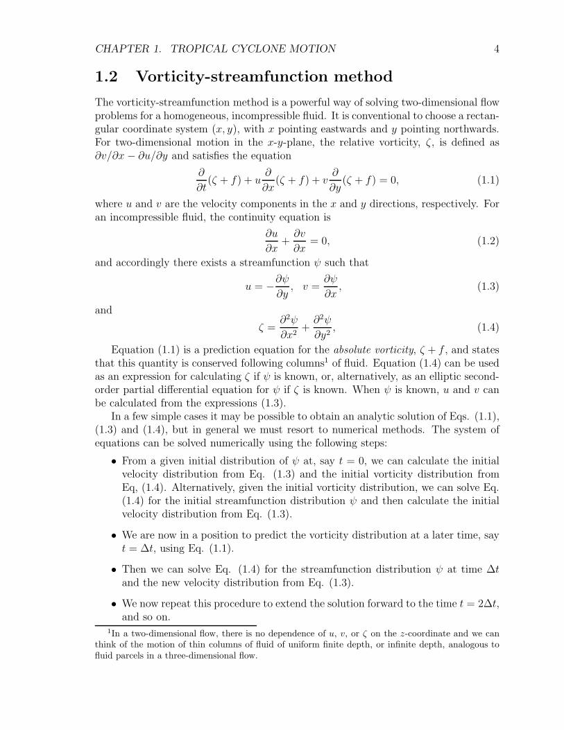
The vorticity-streamfunction method is a powerful way of solving two-dimensional flowproblems for a homogeneous, incompressible fluid. It is conventional to choose a rectan-gular coordinate system (x, y), with x pointing eastwards and y pointing northwards.For two-dimensional motion in the x-y-plane, the relative vorticity, ζ , is defined as∂v/∂x − ∂u/∂y and satisfies the equation

∂

∂t(ζ + f) + u

∂

∂x(ζ + f) + v

∂

∂y(ζ + f) = 0, (1.1)

where u and v are the velocity components in the x and y directions, respectively. Foran incompressible fluid, the continuity equation is

∂u

∂x+∂v

∂x= 0, (1.2)

and accordingly there exists a streamfunction ψ such that

u = −∂ψ∂y, v =

∂ψ

∂x, (1.3)

and

ζ =∂2ψ

∂x2+∂2ψ

∂y2, (1.4)

Equation (1.1) is a prediction equation for the absolute vorticity, ζ + f , and statesthat this quantity is conserved following columns1 of fluid. Equation (1.4) can be usedas an expression for calculating ζ if ψ is known, or, alternatively, as an elliptic second-order partial differential equation for ψ if ζ is known. When ψ is known, u and v canbe calculated from the expressions (1.3).

In a few simple cases it may be possible to obtain an analytic solution of Eqs. (1.1),(1.3) and (1.4), but in general we must resort to numerical methods. The system ofequations can be solved numerically using the following steps:

• From a given initial distribution of ψ at, say t = 0, we can calculate the initialvelocity distribution from Eq. (1.3) and the initial vorticity distribution fromEq, (1.4). Alternatively, given the initial vorticity distribution, we can solve Eq.(1.4) for the initial streamfunction distribution ψ and then calculate the initialvelocity distribution from Eq. (1.3).

• We are now in a position to predict the vorticity distribution at a later time, sayt = Δt, using Eq. (1.1).

• Then we can solve Eq. (1.4) for the streamfunction distribution ψ at time Δtand the new velocity distribution from Eq. (1.3).

• We now repeat this procedure to extend the solution forward to the time t = 2Δt,and so on.

1In a two-dimensional flow, there is no dependence of u, v, or ζ on the z-coordinate and we canthink of the motion of thin columns of fluid of uniform finite depth, or infinite depth, analogous tofluid parcels in a three-dimensional flow.


1.3 The partitioning problem

An important issue that arises in the study of tropical cyclone motion is the so-calledpartitioning problem, i.e. the problem of deciding what is the cyclone and what is itsenvironment. Of course, Nature makes no distinction so that any partitioning thatwe make to enable us to discuss the interaction between the tropical cyclone and itsenvironment is necessarily non-unique.

Various methods have been proposed to isolate the cyclone from its environmentand each may have their merits in different applications. One obvious possibility isto define the cyclone as the azimuthally-averaged flow about the vortex centre, andthe residual flow (i.e. the asymmetric component) as ”the environment”. But thenthe question arises: which centre? We show below that, in general, the location ofthe minimum surface pressure and the centre of the vortex circulation at any levelare not coincident in general. Many theoretical studies consider the motion of aninitially symmetric vortex in some analytically-prescribed environmental flow. If theflow is assumed to be barotropic, there is no mechanism to change the vorticity of aircolumns as they move around. In this case it is advantageous to define the vortex tobe the initial relative vorticity distribution, appropriately relocated, in which case allthe flow changes accompanying the vortex motion reside in the residual flow that isconsidered to be the vortex environment. We choose also the position of the relativevorticity maximum as the ’appropriate location’ for the vortex. An advantage of thismethod is that all the subsequent flow changes are contained in one component of thepartition and the vortex remains ”well-behaved” at large radial distances. Further, onedoes not have to be concerned with vorticity transfer between the symmetric vortexand the environment as this is zero, by definition. The method has advantages also forunderstanding the motion of initially asymmetric vortices in Section 2.1.

The partitioning method can be illustrated mathematically as follows. Let the totalwind be expressed as u = us + U, where us denotes the symmetric velocity field andU is the velocity associated with the vortex environment. We define correspondingvorticities ζs = k · ∇∧us and Γ = k · ∇∧U, where k is the unit vector in the vertical.Then Eq. (1.1) can be partitioned into two equations:

∂ζs∂t

+ c(t) · ∇ζs = 0, (1.5)

and∂Γ

∂t= −us · ∇(Γ + f) − (U − c) · ∇ζs −U · ∇(Γ + f), (1.6)

Note that us · ∇ζs = 0, because for a symmetric vortex us is normal to ∇ζs. Equation(1.5) states that the symmetric vortex translates with speed c and Eq. (1.6) is anequation for the evolution of the asymmetric vorticity. Having solved the latter equa-tion for Γ(x, t), we can obtain the corresponding asymmetric streamfunction by solvingEq. (1.4) in the form ∇2ψa = Γ. The vortex translation velocity c may be obtainedby calculating the speed Uc = k ∧ ∇ψa at the vortex centre. In some situations it isadvantageous to transform the equations of motion into a frame of reference moving


with the vortex2. Then Eq. (1.5) becomes ∂ζs/∂t ≡ 0 and the vorticity equation (1.6)becomes

∂Γ

∂t= −us · ∇(Γ + f) − (U − c) · ∇ζs − (U − c) · ∇(Γ + f). (1.7)

1.4 Prototype problems

1.4.1 Symmetric vortex in a uniform flow

Consider a barotropic vortex with an axisymmetric vorticity distribution embedded ina uniform zonal air stream on an f -plane. The streamfunction for the flow has theform:

ψ(x, y) = −Uy + ψ′(r), (1.8)

where r2 = (x− Ut)2 + y2. The corresponding velocity field is

u = (U, 0) +

(−∂ψ

′

∂y,∂ψ′

∂x

), (1.9)

The relative vorticity distribution, ζ = ∇2ψ, is symmetric about the point (x −Ut, 0), which translates with speed U in the x-direction. However, neither the stream-function distribution ψ(x, y, t), nor the pressure distribution p(x, y, t), are symmetricand, in general, the locations of the minimum central pressure, maximum relativevorticity, and minimum streamfunction (where u = 0) do not coincide. In particular,there are three important deductions from (1.9):

• The total velocity field of the translating vortex is not symmetric, and

• The maximum wind speed is simply the arithmetic sum of U and the maximumtangential wind speed of the symmetric vortex, Vm = (∂ψ′/∂r)max.

• The maximum wind speed occurs on the right-hand-side of the vortex in thedirection of motion in the northern hemisphere and on the left-hand-side in thesouthern hemisphere.

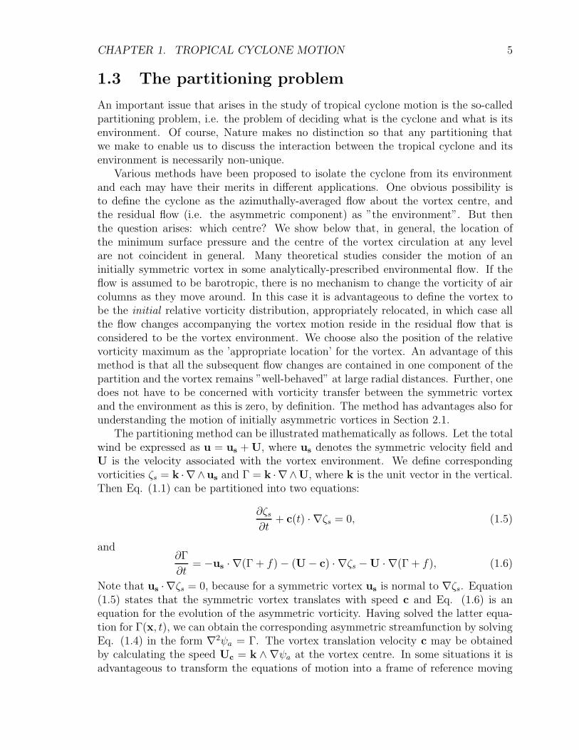
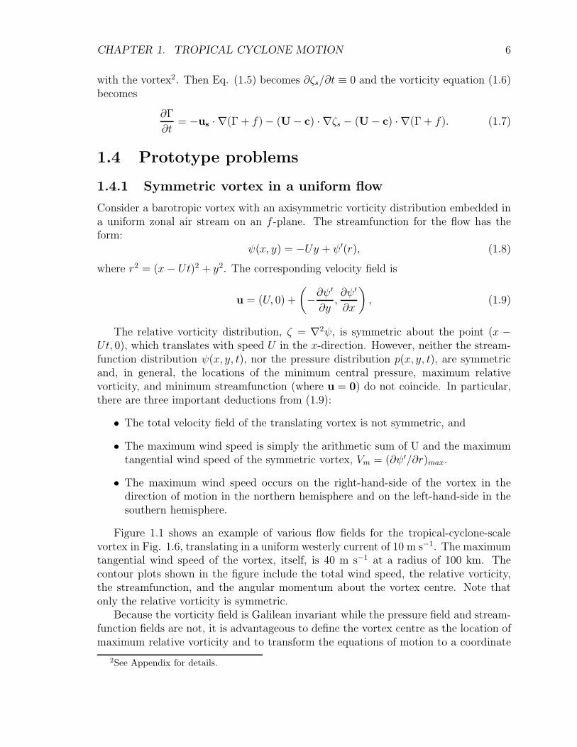
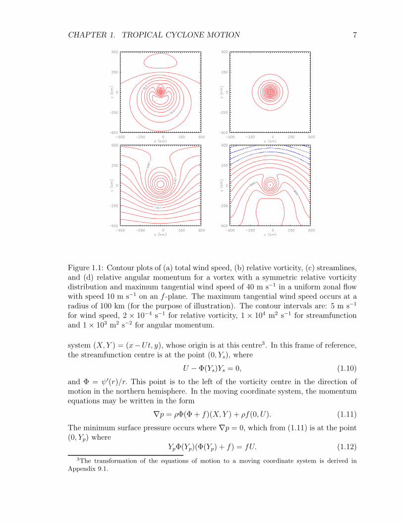
Figure 1.1 shows an example of various flow fields for the tropical-cyclone-scalevortex in Fig. 1.6, translating in a uniform westerly current of 10 m s−1. The maximumtangential wind speed of the vortex, itself, is 40 m s−1 at a radius of 100 km. Thecontour plots shown in the figure include the total wind speed, the relative vorticity,the streamfunction, and the angular momentum about the vortex centre. Note thatonly the relative vorticity is symmetric.

Because the vorticity field is Galilean invariant while the pressure field and stream-function fields are not, it is advantageous to define the vortex centre as the location ofmaximum relative vorticity and to transform the equations of motion to a coordinate

2See Appendix for details.


Figure 1.1: Contour plots of (a) total wind speed, (b) relative vorticity, (c) streamlines,and (d) relative angular momentum for a vortex with a symmetric relative vorticitydistribution and maximum tangential wind speed of 40 m s−1 in a uniform zonal flowwith speed 10 m s−1 on an f -plane. The maximum tangential wind speed occurs at aradius of 100 km (for the purpose of illustration). The contour intervals are: 5 m s−1

for wind speed, 2 × 10−4 s−1 for relative vorticity, 1 × 104 m2 s−1 for streamfunctionand 1 × 103 m2 s−2 for angular momentum.

system (X, Y ) = (x−Ut, y), whose origin is at this centre3. In this frame of reference,the streamfunction centre is at the point (0, Ys), where

U − Φ(Ys)Ys = 0, (1.10)

and Φ = ψ′(r)/r. This point is to the left of the vorticity centre in the direction ofmotion in the northern hemisphere. In the moving coordinate system, the momentumequations may be written in the form

∇p = ρΦ(Φ + f)(X, Y ) + ρf(0, U). (1.11)

The minimum surface pressure occurs where ∇p = 0, which from (1.11) is at the point(0, Yp) where

YpΦ(Yp)(Φ(Yp) + f) = fU. (1.12)

3The transformation of the equations of motion to a moving coordinate system is derived inAppendix 9.1.


We show that, although Yp and Ys are not zero and not equal, they are for practicalpurposes relatively small.

Consider the case where the inner core is in solid body rotation out to the radiusrm, of maximum tangential wind speed vm, with uniform angular velocity Ω = vm/rm.Then ψ′(r) = Ωr and Φ = Ω. It follows readily that Ys/rm = U/vm and Yp/rm =U/(vmRom), where Rom = vm/(rmf) is the Rossby number of the vortex core whichis large compared with unity in a tropical cyclone. Taking typical values: f = 5 ×10−5 s−1, U = 10 m s−1, vm = 50 m s−1, rm = 50 km, Rom = 20 and Ys = 10 km,Yp = 0.5 km, the latter being much smaller than rm. Clearly, for weaker vortices(smaller vm) and/or stronger basic flows (larger U), the values of Ys/rm and Yp/rm arecomparatively larger and the difference between the various centres may be significant.

1.4.2 Vortex motion on a beta-plane

Another prototype problem for tropical-cyclone motion considers the evolution of aninitially-symmetric barotropic vortex on a Northern Hemisphere β-plane in a quiescentenvironment. In this problem, the initial absolute vorticity distribution, ζ + f is notsymmetric about the vortex centre: a fluid parcel at a distance yo poleward of the vortexcentre will have a larger absolute vorticity than one at the same distance equatorwardsof the centre. Now Eq. (1.1) tells us that ζ+ f is conserved following fluid parcels andinitially at least these will move in circular trajectories about the centre. Clearly allparcels initially west of the vortex centre will move equatorwards while those initiallyon the eastward side will move polewards. Since the planetary vorticity decreases forparcels moving equatorwards, their relative vorticity must increase and conversely forparcels moving polewards. Thus we expect to find a cyclonic vorticity anomaly to thewest of the vortex and an anticyclonic anomaly to the east.

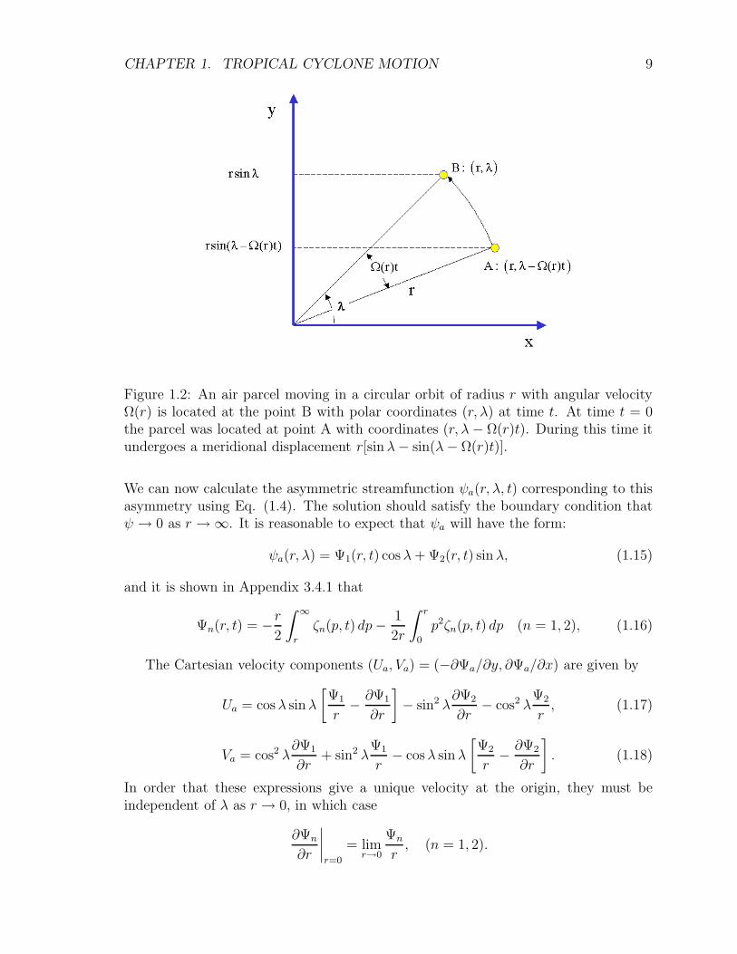
To a first approximation we can determine the evolution of the vorticity asymme-tries by assuming that the flow about the vortex motion remains circular relative to themoving vortex (we discuss the reason for the vortex movement below). Consider an airparcel that at time t is at the point with polar coordinate (r, λ) located at the (moving)vortex centre (Fig. 1.2). This parcel would have been at the position (r, λ − Ω(r)t)at the initial instant, where Ω(r) = V (r)/r is the angular velocity at radius r andV (r) is the tangential wind speed at that radius. The initial vorticity of the parcel isζs(r) + f0 + βr sin(λ − Ω(r)t) while the vorticity of a parcel at its current location isζ(r) + f0 + βr sin λ. Therefore the vorticity perturbation ζa(r, λ) at the point (r, λ) attime t is ζ(r) − ζs(r), or

ζa(r, λ) = βr[sinλ− sin(λ− Ω(r)t)]

orζa(r, λ) = ζ1(r, t) cosλ+ ζ2(r, t) sinλ, (1.13)

whereζ1(r, t) = −βr sin(Ω(r)t), ζ2(r, t) = −βr[1 − cos(Ω(r)t)]. (1.14)


Figure 1.2: An air parcel moving in a circular orbit of radius r with angular velocityΩ(r) is located at the point B with polar coordinates (r, λ) at time t. At time t = 0the parcel was located at point A with coordinates (r, λ− Ω(r)t). During this time itundergoes a meridional displacement r[sinλ− sin(λ− Ω(r)t)].

We can now calculate the asymmetric streamfunction ψa(r, λ, t) corresponding to thisasymmetry using Eq. (1.4). The solution should satisfy the boundary condition thatψ → 0 as r → ∞. It is reasonable to expect that ψa will have the form:

ψa(r, λ) = Ψ1(r, t) cosλ+ Ψ2(r, t) sinλ, (1.15)

and it is shown in Appendix 3.4.1 that

Ψn(r, t) = −r2

∫ ∞

r

ζn(p, t) dp− 1

2r

∫ r

0

p2ζn(p, t) dp (n = 1, 2), (1.16)

The Cartesian velocity components (Ua, Va) = (−∂Ψa/∂y, ∂Ψa/∂x) are given by

Ua = cosλ sinλ

[Ψ1

r− ∂Ψ1

∂r

]− sin2 λ

∂Ψ2

∂r− cos2 λ

Ψ2

r, (1.17)

Va = cos2 λ∂Ψ1

∂r+ sin2 λ

Ψ1

r− cosλ sinλ

[Ψ2

r− ∂Ψ2

∂r

]. (1.18)

In order that these expressions give a unique velocity at the origin, they must beindependent of λ as r → 0, in which case

∂Ψn

∂r

∣∣∣∣r=0

= limr→0

Ψn

r, (n = 1, 2).


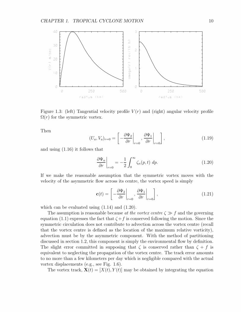
Figure 1.3: (left) Tangential velocity profile V (r) and (right) angular velocity profileΩ(r) for the symmetric vortex.

Then

(Ua, Va)r=0 =

[−∂Ψ2

∂r

∣∣∣∣r=0

,∂Ψ1

∂r

∣∣∣∣r=0

], (1.19)

and using (1.16) it follows that

∂Ψn

∂r

∣∣∣∣r=0

= −1

2

∫ ∞

0

ζn(p, t) dp. (1.20)

If we make the reasonable assumption that the symmetric vortex moves with thevelocity of the asymmetric flow across its centre, the vortex speed is simply

c(t) =

[−∂Ψ2

∂r

∣∣∣∣r=0

,∂Ψ1

∂r

∣∣∣∣r=0

], (1.21)

which can be evaluated using (1.14) and (1.20).The assumption is reasonable because at the vortex centre ζ � f and the governing

equation (1.1) expresses the fact that ζ+f is conserved following the motion. Since thesymmetric circulation does not contribute to advection across the vortex centre (recallthat the vortex centre is defined as the location of the maximum relative vorticity),advection must be by the asymmetric component. With the method of partitioningdiscussed in section 1.2, this component is simply the environmental flow by definition.The slight error committed in supposing that ζ is conserved rather than ζ + f isequivalent to neglecting the propagation of the vortex centre. The track error amountsto no more than a few kilometers per day which is negligible compared with the actualvortex displacements (e.g., see Fig. 1.6).

The vortex track, X(t) = [X(t), Y (t)] may be obtained by integrating the equation


dX/dt = c(t), and using (1.20) and (1.21), we obtain

[X(t)Y (t)

]=

⎡⎣ 1

2

∫∞0

{∫ 1

0ζ2(p, t)dt

}dp

−12

∫∞0

{∫ 1

0ζ1(p, t)dt

}dp

⎤⎦ . (1.22)

With the expressions for ζn in (1.14), this expression reduces to

[X(t)Y (t)

]=

⎡⎣ −1

2β∫∞

0r[t− sin(Ω(r)t)

Ω(r)

]dr

12β∫∞

0r[

1−cos(Ω(r)t)Ω(r)

]dr

⎤⎦ . (1.23)

This expression determines the vortex track in terms of the initial angular velocityprofile of the vortex. To illustrate the solutions we choose the vortex profile shown inFig. 1.3. The velocity profile V (r) and corresponding angular velocity profile Ω(r) areshown as solid lines in Fig. 1.3. The maximum wind speed of 40 m s−1 occurs at aradius of 100 km and the region of approximate gale force winds (> 15 m s−1) extendsto 300 km. The angular velocity has a maximum at the vortex center and decreasesmonotonically with radius. Figure 1.4 shows the asymmetric vorticity field calculatedfrom (1.14) and the corresponding streamfunction field from (1.16) at selected times,while Fig. 1.5 compares the analytical solutions with numerical solutions at 24 h.

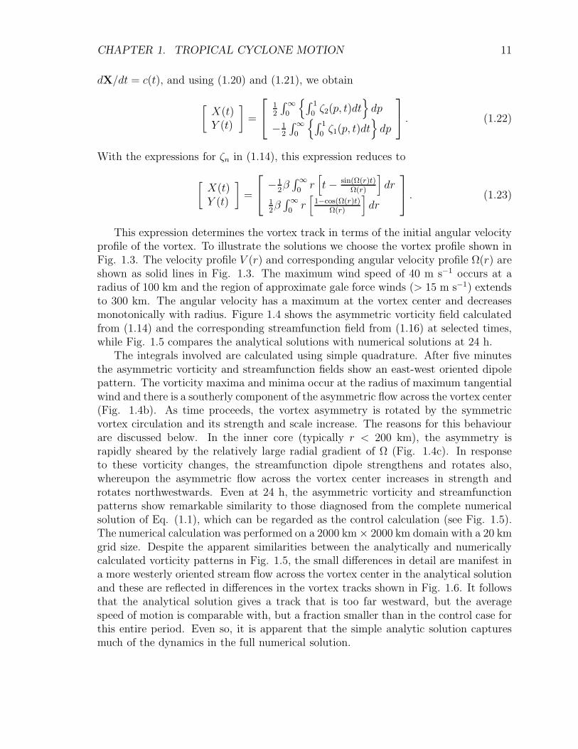
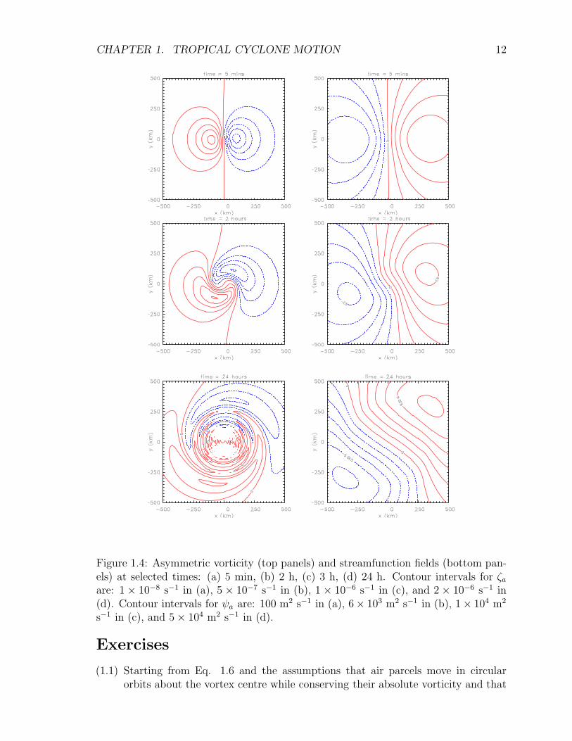
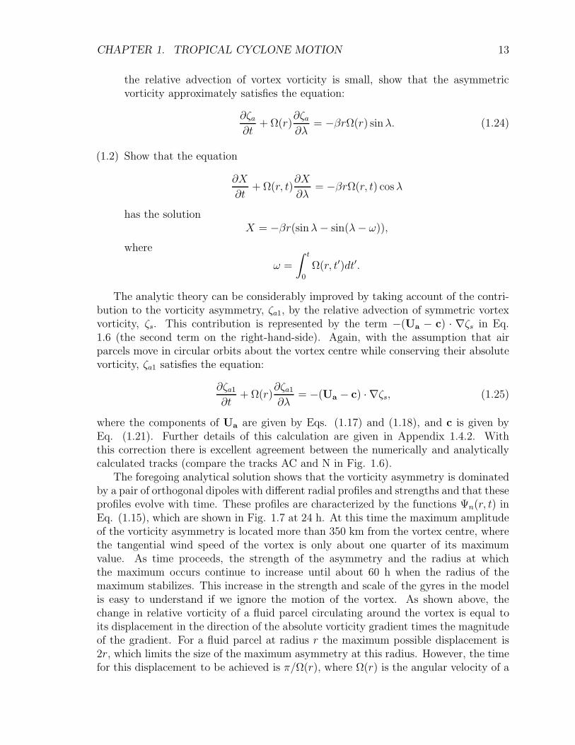
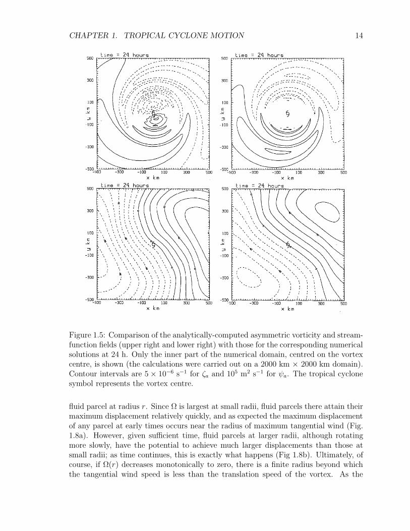
The integrals involved are calculated using simple quadrature. After five minutesthe asymmetric vorticity and streamfunction fields show an east-west oriented dipolepattern. The vorticity maxima and minima occur at the radius of maximum tangentialwind and there is a southerly component of the asymmetric flow across the vortex center(Fig. 1.4b). As time proceeds, the vortex asymmetry is rotated by the symmetricvortex circulation and its strength and scale increase. The reasons for this behaviourare discussed below. In the inner core (typically r < 200 km), the asymmetry israpidly sheared by the relatively large radial gradient of Ω (Fig. 1.4c). In responseto these vorticity changes, the streamfunction dipole strengthens and rotates also,whereupon the asymmetric flow across the vortex center increases in strength androtates northwestwards. Even at 24 h, the asymmetric vorticity and streamfunctionpatterns show remarkable similarity to those diagnosed from the complete numericalsolution of Eq. (1.1), which can be regarded as the control calculation (see Fig. 1.5).The numerical calculation was performed on a 2000 km × 2000 km domain with a 20 kmgrid size. Despite the apparent similarities between the analytically and numericallycalculated vorticity patterns in Fig. 1.5, the small differences in detail are manifest ina more westerly oriented stream flow across the vortex center in the analytical solutionand these are reflected in differences in the vortex tracks shown in Fig. 1.6. It followsthat the analytical solution gives a track that is too far westward, but the averagespeed of motion is comparable with, but a fraction smaller than in the control case forthis entire period. Even so, it is apparent that the simple analytic solution capturesmuch of the dynamics in the full numerical solution.


Figure 1.4: Asymmetric vorticity (top panels) and streamfunction fields (bottom pan-els) at selected times: (a) 5 min, (b) 2 h, (c) 3 h, (d) 24 h. Contour intervals for ζaare: 1 × 10−8 s−1 in (a), 5 × 10−7 s−1 in (b), 1 × 10−6 s−1 in (c), and 2 × 10−6 s−1 in(d). Contour intervals for ψa are: 100 m2 s−1 in (a), 6× 103 m2 s−1 in (b), 1× 104 m2

s−1 in (c), and 5 × 104 m2 s−1 in (d).

Exercises

(1.1) Starting from Eq. 1.6 and the assumptions that air parcels move in circularorbits about the vortex centre while conserving their absolute vorticity and that


the relative advection of vortex vorticity is small, show that the asymmetricvorticity approximately satisfies the equation:

∂ζa∂t

+ Ω(r)∂ζa∂λ

= −βrΩ(r) sinλ. (1.24)

(1.2) Show that the equation

∂X

∂t+ Ω(r, t)

∂X

∂λ= −βrΩ(r, t) cosλ

has the solutionX = −βr(sinλ− sin(λ− ω)),

where

ω =

∫ t

0

Ω(r, t′)dt′.

The analytic theory can be considerably improved by taking account of the contri-bution to the vorticity asymmetry, ζa1, by the relative advection of symmetric vortexvorticity, ζs. This contribution is represented by the term −(Ua − c) · ∇ζs in Eq.1.6 (the second term on the right-hand-side). Again, with the assumption that airparcels move in circular orbits about the vortex centre while conserving their absolutevorticity, ζa1 satisfies the equation:

∂ζa1

∂t+ Ω(r)

∂ζa1

∂λ= −(Ua − c) · ∇ζs, (1.25)

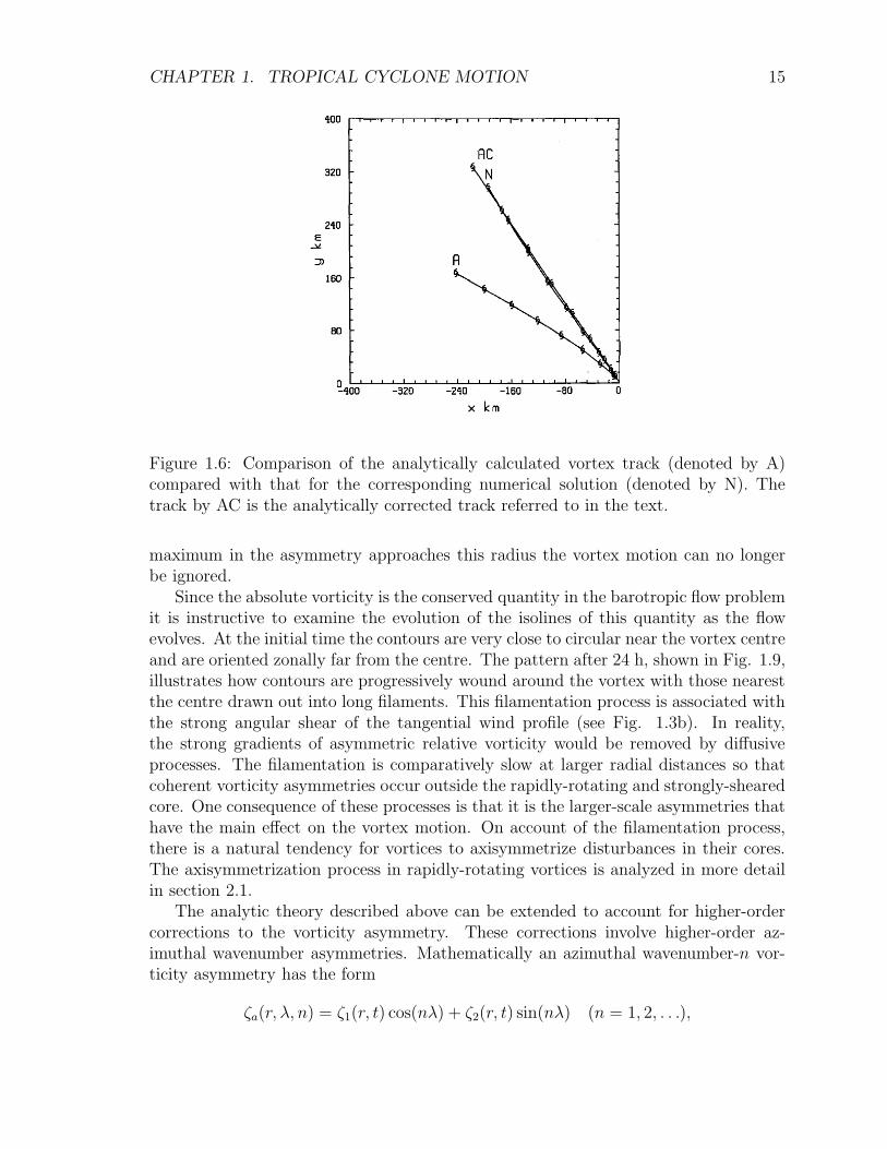
where the components of Ua are given by Eqs. (1.17) and (1.18), and c is given byEq. (1.21). Further details of this calculation are given in Appendix 1.4.2. Withthis correction there is excellent agreement between the numerically and analyticallycalculated tracks (compare the tracks AC and N in Fig. 1.6).

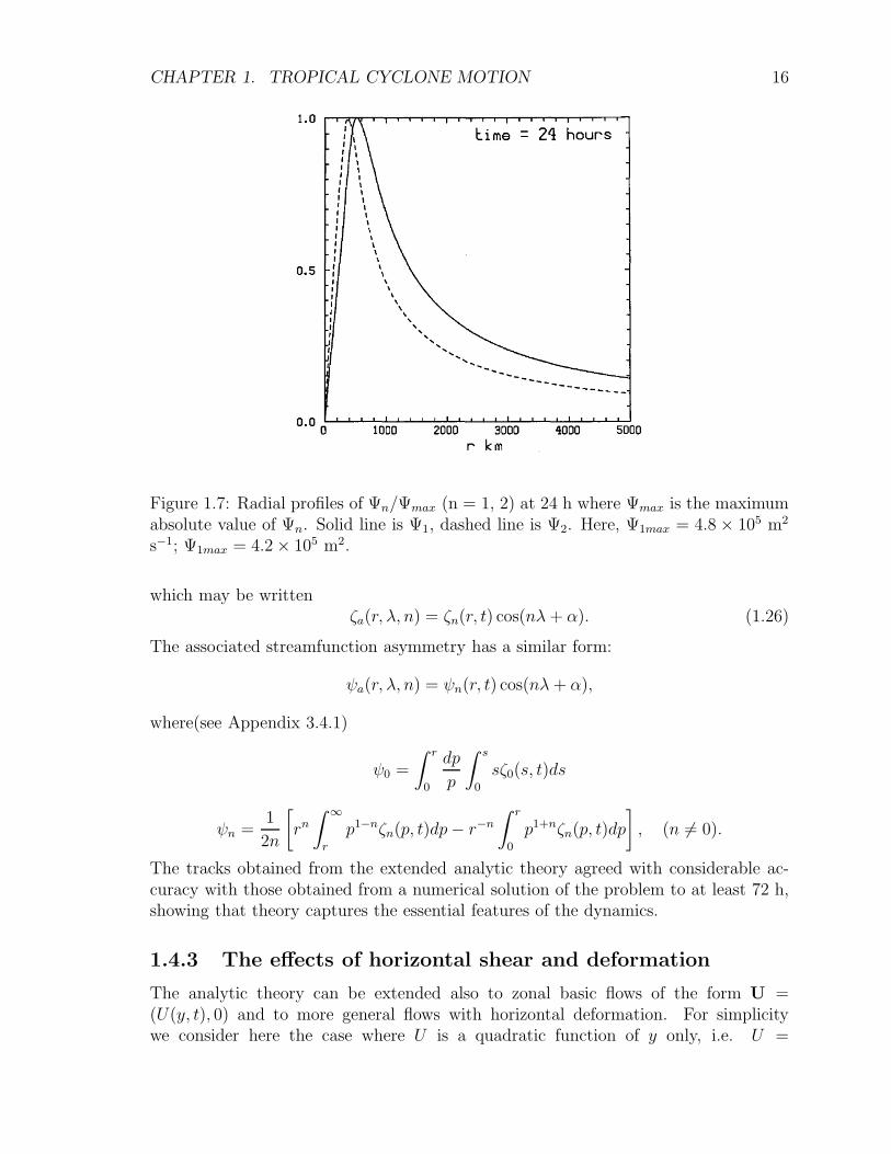
The foregoing analytical solution shows that the vorticity asymmetry is dominatedby a pair of orthogonal dipoles with different radial profiles and strengths and that theseprofiles evolve with time. These profiles are characterized by the functions Ψn(r, t) inEq. (1.15), which are shown in Fig. 1.7 at 24 h. At this time the maximum amplitudeof the vorticity asymmetry is located more than 350 km from the vortex centre, wherethe tangential wind speed of the vortex is only about one quarter of its maximumvalue. As time proceeds, the strength of the asymmetry and the radius at whichthe maximum occurs continue to increase until about 60 h when the radius of themaximum stabilizes. This increase in the strength and scale of the gyres in the modelis easy to understand if we ignore the motion of the vortex. As shown above, thechange in relative vorticity of a fluid parcel circulating around the vortex is equal toits displacement in the direction of the absolute vorticity gradient times the magnitudeof the gradient. For a fluid parcel at radius r the maximum possible displacement is2r, which limits the size of the maximum asymmetry at this radius. However, the timefor this displacement to be achieved is π/Ω(r), where Ω(r) is the angular velocity of a


Figure 1.5: Comparison of the analytically-computed asymmetric vorticity and stream-function fields (upper right and lower right) with those for the corresponding numericalsolutions at 24 h. Only the inner part of the numerical domain, centred on the vortexcentre, is shown (the calculations were carried out on a 2000 km × 2000 km domain).Contour intervals are 5 × 10−6 s−1 for ζa and 105 m2 s−1 for ψa. The tropical cyclonesymbol represents the vortex centre.

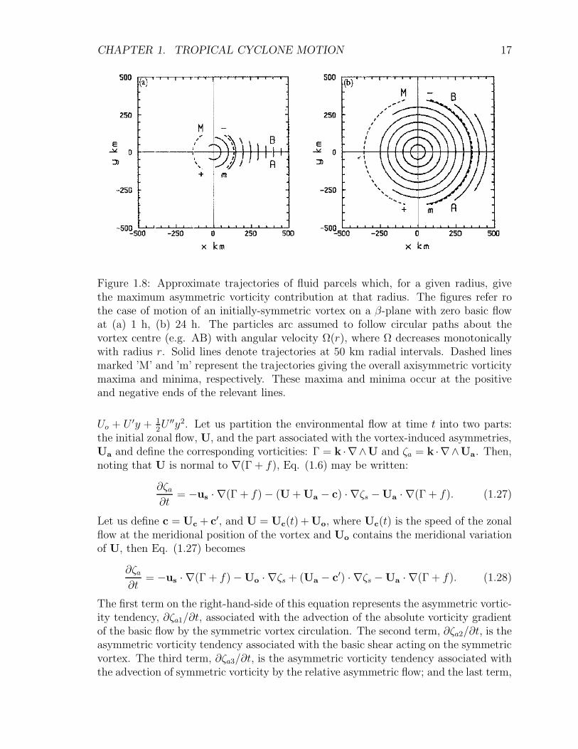
fluid parcel at radius r. Since Ω is largest at small radii, fluid parcels there attain theirmaximum displacement relatively quickly, and as expected the maximum displacementof any parcel at early times occurs near the radius of maximum tangential wind (Fig.1.8a). However, given sufficient time, fluid parcels at larger radii, although rotatingmore slowly, have the potential to achieve much larger displacements than those atsmall radii; as time continues, this is exactly what happens (Fig 1.8b). Ultimately, ofcourse, if Ω(r) decreases monotonically to zero, there is a finite radius beyond whichthe tangential wind speed is less than the translation speed of the vortex. As the


Figure 1.6: Comparison of the analytically calculated vortex track (denoted by A)compared with that for the corresponding numerical solution (denoted by N). Thetrack by AC is the analytically corrected track referred to in the text.

maximum in the asymmetry approaches this radius the vortex motion can no longerbe ignored.

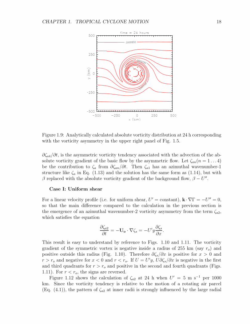
Since the absolute vorticity is the conserved quantity in the barotropic flow problemit is instructive to examine the evolution of the isolines of this quantity as the flowevolves. At the initial time the contours are very close to circular near the vortex centreand are oriented zonally far from the centre. The pattern after 24 h, shown in Fig. 1.9,illustrates how contours are progressively wound around the vortex with those nearestthe centre drawn out into long filaments. This filamentation process is associated withthe strong angular shear of the tangential wind profile (see Fig. 1.3b). In reality,the strong gradients of asymmetric relative vorticity would be removed by diffusiveprocesses. The filamentation is comparatively slow at larger radial distances so thatcoherent vorticity asymmetries occur outside the rapidly-rotating and strongly-shearedcore. One consequence of these processes is that it is the larger-scale asymmetries thathave the main effect on the vortex motion. On account of the filamentation process,there is a natural tendency for vortices to axisymmetrize disturbances in their cores.The axisymmetrization process in rapidly-rotating vortices is analyzed in more detailin section 2.1.

The analytic theory described above can be extended to account for higher-ordercorrections to the vorticity asymmetry. These corrections involve higher-order az-imuthal wavenumber asymmetries. Mathematically an azimuthal wavenumber-n vor-ticity asymmetry has the form

ζa(r, λ, n) = ζ1(r, t) cos(nλ) + ζ2(r, t) sin(nλ) (n = 1, 2, . . .),


Figure 1.7: Radial profiles of Ψn/Ψmax (n = 1, 2) at 24 h where Ψmax is the maximumabsolute value of Ψn. Solid line is Ψ1, dashed line is Ψ2. Here, Ψ1max = 4.8 × 105 m2

s−1; Ψ1max = 4.2 × 105 m2.

which may be writtenζa(r, λ, n) = ζn(r, t) cos(nλ + α). (1.26)

The associated streamfunction asymmetry has a similar form:

ψa(r, λ, n) = ψn(r, t) cos(nλ+ α),

where(see Appendix 3.4.1)

ψ0 =

∫ r

0

dp

p

∫ s

0

sζ0(s, t)ds

ψn =1

2n

[rn

∫ ∞

r

p1−nζn(p, t)dp− r−n

∫ r

0

p1+nζn(p, t)dp

], (n �= 0).

The tracks obtained from the extended analytic theory agreed with considerable ac-curacy with those obtained from a numerical solution of the problem to at least 72 h,showing that theory captures the essential features of the dynamics.

1.4.3 The effects of horizontal shear and deformation

The analytic theory can be extended also to zonal basic flows of the form U =(U(y, t), 0) and to more general flows with horizontal deformation. For simplicitywe consider here the case where U is a quadratic function of y only, i.e. U =


Figure 1.8: Approximate trajectories of fluid parcels which, for a given radius, givethe maximum asymmetric vorticity contribution at that radius. The figures refer rothe case of motion of an initially-symmetric vortex on a β-plane with zero basic flowat (a) 1 h, (b) 24 h. The particles arc assumed to follow circular paths about thevortex centre (e.g. AB) with angular velocity Ω(r), where Ω decreases monotonicallywith radius r. Solid lines denote trajectories at 50 km radial intervals. Dashed linesmarked ’M’ and ’m’ represent the trajectories giving the overall axisymmetric vorticitymaxima and minima, respectively. These maxima and minima occur at the positiveand negative ends of the relevant lines.

Uo + U ′y + 12U ′′y2. Let us partition the environmental flow at time t into two parts:

the initial zonal flow, U, and the part associated with the vortex-induced asymmetries,Ua and define the corresponding vorticities: Γ = k ·∇∧U and ζa = k ·∇∧Ua. Then,noting that U is normal to ∇(Γ + f), Eq. (1.6) may be written:

∂ζa∂t

= −us · ∇(Γ + f) − (U + Ua − c) · ∇ζs −Ua · ∇(Γ + f). (1.27)

Let us define c = Uc + c′, and U = Uc(t) + Uo, where Uc(t) is the speed of the zonalflow at the meridional position of the vortex and Uo contains the meridional variationof U, then Eq. (1.27) becomes

∂ζa∂t

= −us · ∇(Γ + f) − Uo · ∇ζs + (Ua − c′) · ∇ζs − Ua · ∇(Γ + f). (1.28)

The first term on the right-hand-side of this equation represents the asymmetric vortic-ity tendency, ∂ζa1/∂t, associated with the advection of the absolute vorticity gradientof the basic flow by the symmetric vortex circulation. The second term, ∂ζa2/∂t, is theasymmetric vorticity tendency associated with the basic shear acting on the symmetricvortex. The third term, ∂ζa3/∂t, is the asymmetric vorticity tendency associated withthe advection of symmetric vorticity by the relative asymmetric flow; and the last term,


Figure 1.9: Analytically calculated absolute vorticity distribution at 24 h correspondingwith the vorticity asymmetry in the upper right panel of Fig. 1.5.

∂ζa4/∂t, is the asymmetric vorticity tendency associated with the advection of the ab-solute vorticity gradient of the basic flow by the asymmetric flow. Let ζan(n = 1 . . . 4)be the contribution to ζa from ∂ζan/∂t. Then ζa1 has an azimuthal wavenumber-1structure like ζa in Eq. (1.13) and the solution has the same form as (1.14), but withβ replaced with the absolute vorticity gradient of the background flow, β − U ′′.

Case I: Uniform shear

For a linear velocity profile (i.e. for uniform shear, U ′ = constant), k ·∇Γ = −U ′′ = 0,so that the main difference compared to the calculation in the previous section isthe emergence of an azimuthal wavenumber-2 vorticity asymmetry from the term ζa2,which satisfies the equation

∂ζa2

∂t= −Uo · ∇ζs = −U ′y

∂ζs∂x

.

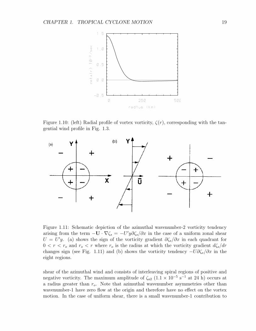
This result is easy to understand by reference to Figs. 1.10 and 1.11. The vorticitygradient of the symmetric vortex is negative inside a radius of 255 km (say ro) andpositive outside this radius (Fig. 1.10). Therefore ∂ζs/∂x is positive for x > 0 andr > ro and negative for x < 0 and r < ro. If U = U ′y, U∂ζs/∂x is negative in the firstand third quadrants for r > ro and positive in the second and fourth quadrants (Figs.1.11). For r < ro, the signs are reversed.

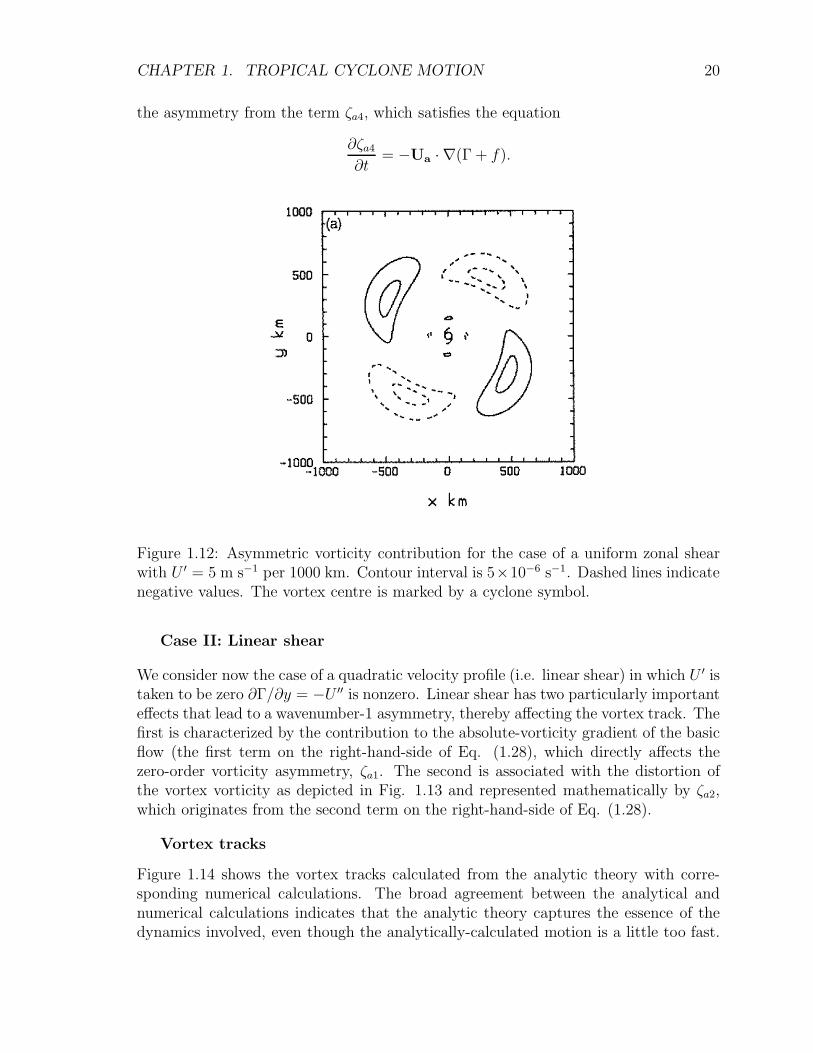
Figure 1.12 shows the calculation of ζa2 at 24 h when U ′ = 5 m s−1 per 1000km. Since the vorticity tendency is relative to the motion of a rotating air parcel(Eq. (4.1)), the pattern of ζa2 at inner radii is strongly influenced by the large radial


Figure 1.10: (left) Radial profile of vortex vorticity, ζ(r), corresponding with the tan-gential wind profile in Fig. 1.3.

Figure 1.11: Schematic depiction of the azimuthal wavenumber-2 vorticity tendencyarising from the term −U · ∇ζs = −U ′y∂ζs/∂x in the case of a uniform zonal shearU = U ′y. (a) shows the sign of the vorticity gradient ∂ζs/∂x in each quadrant for0 < r < ro and ro < r where ro is the radius at which the vorticity gradient dζs/drchanges sign (see Fig. 1.11) and (b) shows the vorticity tendency −U∂ζs/∂x in theeight regions.

shear of the azimuthal wind and consists of interleaving spiral regions of positive andnegative vorticity. The maximum amplitude of ζa2 (1.1 × 10−5 s−1 at 24 h) occurs ata radius greater than ro. Note that azimuthal wavenumber asymmetries other thanwavenumber-1 have zero flow at the origin and therefore have no effect on the vortexmotion. In the case of uniform shear, there is a small wavenumber-1 contribution to


the asymmetry from the term ζa4, which satisfies the equation

∂ζa4

∂t= −Ua · ∇(Γ + f).

Figure 1.12: Asymmetric vorticity contribution for the case of a uniform zonal shearwith U ′ = 5 m s−1 per 1000 km. Contour interval is 5×10−6 s−1. Dashed lines indicatenegative values. The vortex centre is marked by a cyclone symbol.

Case II: Linear shear

We consider now the case of a quadratic velocity profile (i.e. linear shear) in which U ′ istaken to be zero ∂Γ/∂y = −U ′′ is nonzero. Linear shear has two particularly importanteffects that lead to a wavenumber-1 asymmetry, thereby affecting the vortex track. Thefirst is characterized by the contribution to the absolute-vorticity gradient of the basicflow (the first term on the right-hand-side of Eq. (1.28), which directly affects thezero-order vorticity asymmetry, ζa1. The second is associated with the distortion ofthe vortex vorticity as depicted in Fig. 1.13 and represented mathematically by ζa2,which originates from the second term on the right-hand-side of Eq. (1.28).

Vortex tracks

Figure 1.14 shows the vortex tracks calculated from the analytic theory with corre-sponding numerical calculations. The broad agreement between the analytical andnumerical calculations indicates that the analytic theory captures the essence of thedynamics involved, even though the analytically-calculated motion is a little too fast.


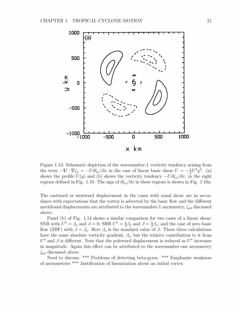
Figure 1.13: Schematic depiction of the wavenumber-1 vorticity tendency arising fromthe term −U · ∇ζs = −U∂ζs/∂x in the case of linear basic shear U = −1

2U ′′y2. (a)

shows the profile U(y) and (b) shows the vorticity tendency −U∂ζs/∂x, in the eightregions defined in Fig. 1.10. The sign of ∂ζs/∂x in these regions is shown in Fig. 1.10a.

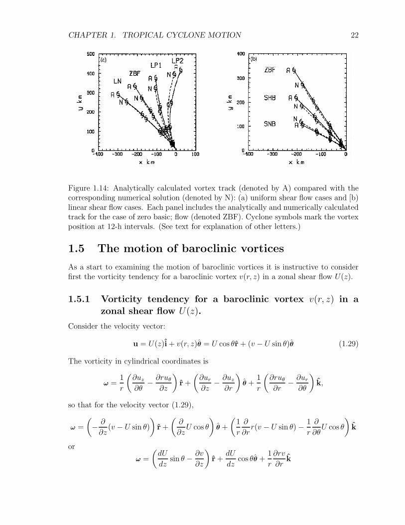
The eastward or westward displacement in the cases with zonal shear are in accor-dance with expectations that the vortex is advected by the basic flow and the differentmeridional displacements are attributed to the wavenumber-1 asymmetry, ζa4 discussedabove.

Panel (b) of Fig. 1.14 shows a similar comparison for two cases of a linear shear:SNB with U ′′ = βo and β = 0; SHB U ′′ = 1

2βo and β = 1

2βo; and the case of zero basic

flow (ZBF) with β = βo. Here βo is the standard value of β. These three calculationshave the same absolute vorticity gradient, βo, but the relative contribution to it fromU ′′ and β is different. Note that the poleward displacement is reduced as U ′′ increasesin magnitude. Again this effect can be attributed to the wavenumber-one asymmetryζa2 discussed above.

Need to discuss: *** Problems of detecting beta-gyres. *** Emphasize weaknessof asymmetries *** Justification of linearization about an initial vortex


Figure 1.14: Analytically calculated vortex track (denoted by A) compared with thecorresponding numerical solution (denoted by N): (a) uniform shear flow cases and [b)linear shear flow cases. Each panel includes the analytically and numerically calculatedtrack for the case of zero basic; flow (denoted ZBF). Cyclone symbols mark the vortexposition at 12-h intervals. (See text for explanation of other letters.)

1.5 The motion of baroclinic vortices

As a start to examining the motion of baroclinic vortices it is instructive to considerfirst the vorticity tendency for a baroclinic vortex v(r, z) in a zonal shear flow U(z).

1.5.1 Vorticity tendency for a baroclinic vortex v(r, z) in a

zonal shear flow U(z).

Consider the velocity vector:

u = U(z)̂i + v(r, z)θ̂ = U cos θr̂ + (v − U sin θ)θ̂ (1.29)

The vorticity in cylindrical coordinates is

ω =1

r

(∂uz

∂θ− ∂ruθ

∂z

)r̂ +

(∂ur

∂z− ∂uz

∂r

)θ̂ +

1

r

(∂ruθ

∂r− ∂ur

∂θ

)k̂,

so that for the velocity vector (1.29),

ω =

(− ∂

∂z(v − U sin θ)

)r̂ +

(∂

∂zU cos θ

)θ̂ +

(1

r

∂

∂rr(v − U sin θ) − 1

r

∂

∂θU cos θ

)k̂

or

ω =

(dU

dzsin θ − ∂v

∂z

)r̂ +

dU

dzcos θθ̂ +

1

r

∂rv

∂rk̂


Let us write

ω =

(ξ +

dU

dzsin θ

)r̂ +

dU

dzcos θθ̂ + ζk̂ (1.30)

Now, in cylindrical coordinates (see Batchelor, 1970, p602)

u.∇ω =(u.∇ωr − uθωθ

r

)r̂ +

(u.∇ωθ +

uθωr

r

)θ̂ + (u.∇ωz) k̂

Then for the velocity vector (1.29),

u.∇ω =

(u.∇

(ξ +

dU

dzsin θ

)− uθ

r

dU

dzsin θ

)r̂ +

(u.∇ωθ +

uθ

r

(ξ +

dU

dzsin θ

))θ̂ + (u.∇ζ) k̂

The three components of this equation are:

(u.∇ξ − uθωθ

r

)= U cos θ

∂

∂r

(ξ +

dU

dzsin θ

)

+ (v − U sin θ)1

r

∂

∂θ

(ξ +

dU

dzsin θ

)− (v − U sin θ)

r

dU

dzcos θ

= U cos θ∂ξ

∂r

(u.∇ωθ +

uθωr

r

)= U cos θ

∂

∂r

(dU

dzcos θ

)

+ (v − U sin θ)1

r

∂

∂θ

(dU

dzcos θ

)+

(v − U sin θ)

r

(ξ +

dU

dzsin θ

)

=(v − U sin θ)

rξ

u.∇ωz = U cos θ∂ζ

∂r+

(v − U sin θ)

r

∂ζ

∂θ= U cos θ

∂ζ

∂r

Therefore

u.∇ω = U cos θ∂ξ

∂rr̂ +

(v − U sin θ)

rξθ̂ + U cos θ

∂ζ

∂rk̂ (1.31)

Nowω.∇u =

(ω.∇ur − ωθuθ

r

)r̂ +

(ω.∇uθ +

ωθur

r

)θ̂ + (ω.∇uz) k̂. (1.32)

The first component of this equation is

ω.∇ur − ωθuθ

r=

[(ξ +

dU

dzsin θ

)r̂ +

dU

dzcos θθ̂ + ζk

]×


(∂

∂r(U cos θ)r̂ +

1

r

∂

∂θ(U cos θ)θ̂ +

∂

∂z(U cos θ)k̂

)− v − U sin θ

r

dU

dzcos θ

= −Ur

dU

dzcos θ sin θ + ζ

dU

dzcos θ − v − U sin θ

r

dU

dzcos θ

or, finally

ω.∇ur − ωθuθ

r= ζ

dU

dzcos θ − v

r

dU

dzcos θ =

dv

dr

dU

dzcos θ (1.33)

The second component of (1.33) is

ω.∇uθ +ωθur

r=

[(ξ +

dU

dzsin θ

)r̂ +

dU

dzcos θθ̂ + ζk

]×

[∂

∂r(v − U sin θ)r̂ +

1

r

∂

∂θ(v − U sin θ)θ̂ +

∂

∂z(v − U sin θ)k̂

]+U cos θ

r

dU

dzcos θ

=

[(ξ +

dU

dzsin θ

)r̂ +

dU

dzcos θθ̂ + ζk

]×

[∂v

∂rr̂ − U

rcos θθ̂ +

(∂v

∂z− dU

dzsin θ

)k̂

]+U

r

dU

dzcos2 θ

=

(ξ +

dU

dzsin θ

)∂v

∂r− ζ

(ξ +

dU

dzsin θ

)=

(∂v

∂r− ζ

)(ξ +

dU

dzsin θ

),

or, finally,

ω.∇uθ +ωθur

r= −v

r

(ξ +

dU

dzsin θ

)(1.34)

The third component of (1.33) is simply

ω.∇uz = 0 (1.35)

The (1.32) may be written

ω.∇u =dv

dr

dU

dzcos θr̂ − v

r

(ξ +

dU

dzsin θ

)θ̂ (1.36)

∂ω

∂t= −u·∇ω + ω·∇u

u.∇ω = U cos θ∂ξ

∂rr̂ +

(v − U sin θ)

r

(ξ − dU

dzsin θ

)θ̂ + U cos θ

∂ζ

∂rk̂

∂ω

∂t= −

(U cos θ

∂ξ

∂rr̂ +

(v − U sin θ)

rξθ̂ + U cos θ

∂ζ

∂rk̂

)+

dv

dr

dU

dzcos θr̂ − v

r

(ξ +

dU

dzsin θ

)θ̂


=

(−U ∂ξ

∂r+dv

dr

dU

dz

)cos θr̂ −

[(v

r+

(v − U sin θ)

r

)ξ − v

r

dU

dzsin θ

]θ̂ − U cos θ

∂ζ

∂rk̂,

or finally,

∂ω

∂t=

(−U ∂ξ

∂r+dv

dr

dU

dz

)cos θr̂ −

[(2v

r− U sin θ

r

)ξ +

v

r

dU

dzsin θ

]θ̂ − U cos θ

∂ζ

∂rk̂

(1.37)

Special cases:

1. Uniform flow (U = constant), barotropic vortex, v = v(r) ⇒ ξ = 0

∂ω

∂t= −U cos θ

∂ζ

∂rk̂ ⇒ ∂ζ

∂t= −U ∂ζ

∂x

In this case there is only vertical vorticity and this is simply advected by thebasic flow as discussed in Chapter 1.

2. No basic flow (U = 0), baroclinic vortex, v = v(r, z)

∂ω

∂t= −2v

rξθ̂

∂ξ

∂t= 0,

∂η

∂t= −2v

rξ,

∂ζ

∂t= 0

In this case there are initially two components of vorticity, a radial component andvertical vertical component, but in general, the vortex does not remain stationaryas there is generation of toroidal vorticity. The exception is, of course, when thevortex is in thermal-wind balance in which case there is generation of toroidalvorticity of the opposite sign by the horizontal density gradient so that the netrate-of-generation of toroidal vorticity is everywhere zero.

3. Uniform flow (U = constant), baroclinic vortex, v = v(r, z)

∂ω

∂t= −U cos θ

∂ξ

∂rr̂ −

(2v

r− U sin θ

r

)ξθ̂ − U cos θ

∂ζ

∂rk̂

∂ξ

∂t= −U ∂ξ

∂x

∂η

∂t= −

(2v

r− U sin θ

r

)ξ

∂ζ

∂t= −U ∂ζ

∂x

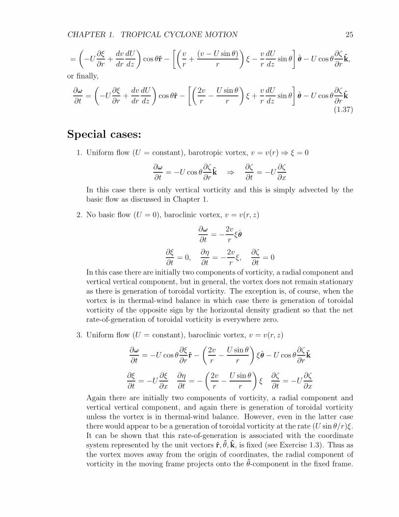
Again there are initially two components of vorticity, a radial component andvertical vertical component, and again there is generation of toroidal vorticityunless the vortex is in thermal-wind balance. However, even in the latter casethere would appear to be a generation of toroidal vorticity at the rate (U sin θ/r)ξ.It can be shown that this rate-of-generation is associated with the coordinatesystem represented by the unit vectors r̂, θ̂, k̂, is fixed (see Exercise 1.3). Thus asthe vortex moves away from the origin of coordinates, the radial component ofvorticity in the moving frame projects onto the θ̂-component in the fixed frame.


4. Uniform shear flow (dU/dz = constant = U ′), barotropic vortex, v = v(r) ⇒ ξ =0

∂ω

∂t=dv

dr

dU

dzcos θr̂ +

v

r

dU

dzsin θθ̂ + U cos θ

∂ζ

∂rk̂

∂ξ

∂t= −U ∂ξ

∂x+dv

dr

dU

dzcos θ

∂η

∂t=v

r

dU

dzsin θ

∂ζ

∂t= −U ∂ζ

∂x

Translation of the balanced density field

Let ρ = p0(r, z) at time t = 0. Then

∂ρ

∂t= −∇ · (ρu) = −u · ∇ρ− ρ(∇ · u).

Now the velocity field u = (U cos θ, v − U sin θ, 0) is nondivergent (∇ · u = 0) andtherefore

∂ρ

∂t= −U cos θ

∂ρ

∂r− (v − U sin θ)

r

∂ρ

∂θ.

The second term on the right-hand-side is zero because ρ is dependent of θ whereupon

∂ρ

∂t= −U ∂ρ

∂x

and the density field is simply advected at speed U .

Exercise 1.3 Show that the term (U sin θ/r)ξ in Eq. (1.37) is the rate-of-generation

of toroidal vorticity in the fixed coordinate system represented by the unit vectors r̂, θ̂, k̂due to the subsequent displacement of the vortex centre from the coordinate origin.

Exercise 1.4 Show that

∂

∂r=

∂

∂x

∂x

∂r+

∂

∂y

∂y

∂r= cos θ

∂

∂x+ sin θ

∂

∂y,

and1

r

∂

∂θ=

1

r

∂

∂x

∂x

∂θ+

1

r

∂

∂y

∂y

∂θ= − sin θ

∂

∂x+ cos θ

∂

∂y,

Deduce that∂

∂x= cos θ

∂

∂r− sin θ

r

∂

∂θ,

and∂

∂y= sin θ

∂

∂r+

cos θ

r

∂

∂θ.


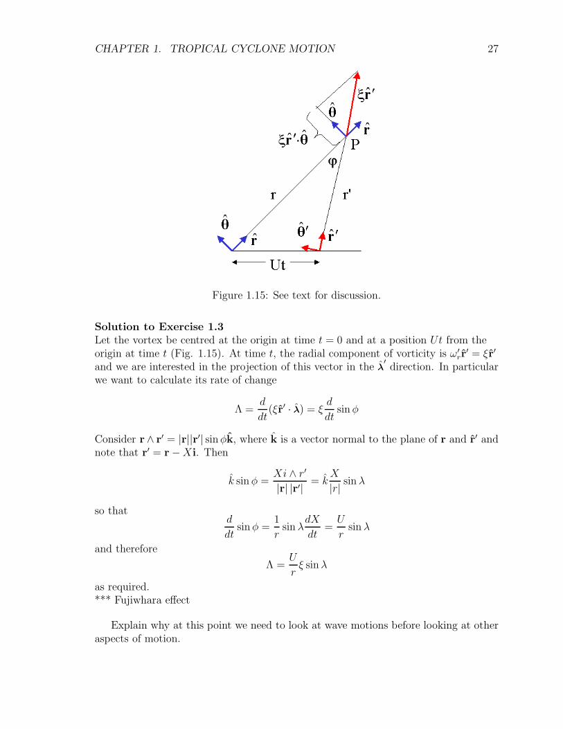
Figure 1.15: See text for discussion.

Solution to Exercise 1.3Let the vortex be centred at the origin at time t = 0 and at a position Ut from theorigin at time t (Fig. 1.15). At time t, the radial component of vorticity is ω′

rr̂′ = ξr̂′

and we are interested in the projection of this vector in the λ̂′direction. In particular

we want to calculate its rate of change

Λ =d

dt(ξr̂′ · λ̂) = ξ

d

dtsinφ

Consider r∧ r′ = |r||r′| sinφk̂, where k̂ is a vector normal to the plane of r and r̂′ andnote that r′ = r −Xi. Then

k̂ sinφ =Xi ∧ r′|r| |r′| = k̂

X

|r| sin λ

so thatd

dtsinφ =

1

rsin λ

dX

dt=U

rsin λ

and therefore

Λ =U

rξ sinλ

as required.*** Fujiwhara effect

Explain why at this point we need to look at wave motions before looking at otheraspects of motion.


1.6 Appendices to Chapter 1

1.6.1 Derivation of Eq. 1.16

We require the solution of ∇2ψa = ζ , when ζa(r, θ) = ζ̂(r)einθ. Now

∇2ψa =∂2ψa

∂r2+

1

r

∂ψa

∂r+

1

r2

∂2ψa

∂θ2= ζ̂(r)einθ

Put ψ = ψ̂(r)einθ, then

d2ψ̂

dr2+

1

r

dψ̂

dr− n2

r2ψ̂ = ζ̂(r). (1.38)

When ζ̂(r) = 0, the equation has solutions ψ̂ = rα where

[α(α− 1) + α− n2]rα−2 = 0,

which givesα2 − n2 = 0 or α = ±n.

Therefore, for a solution of (1.38), try ψ̂ = rnφ(r). Then

ψr = rnφr + nrn−1φ, ψrr = rnφrr + 2nrn−1φr + n(n− 1)rn−2φ (1.39)

whereupon (1.38) gives

rnφrr + 2nrn−1φr + n(n− 1)rn−2φ

+ rn−1φr + nrn−2φ− n2rn−2φ = ζ̂ ,

orrnφrr + (2n+ 1)rn−1φr = ζ̂ .

Multiply by rβ and choose β so that n+ β = 2n+ 1, i.e., β = n+ 1. Thus rn+1 is theintegrating factor. Then

d

dr

[r2n+1φ(r)

]= rn+1ζ̂(r), (1.40)

which may ne integrated to give

r2n+1dφ

dr=

∫ ∞

r

pn+1ζ̂(p)dp+ A,

where A is a constant. Therefore

dφ

dr=

1

r2n+1

∫ ∞

r

pn+1ζ̂(p)dp+A

r2n+1

Finally,

φ =

∫ ∞

r

dq

q2n+1

∫ ∞

q

pn+1ζ̂(p)dp+

∫ ∞

q

Adq

q2n+1+B, (1.41)


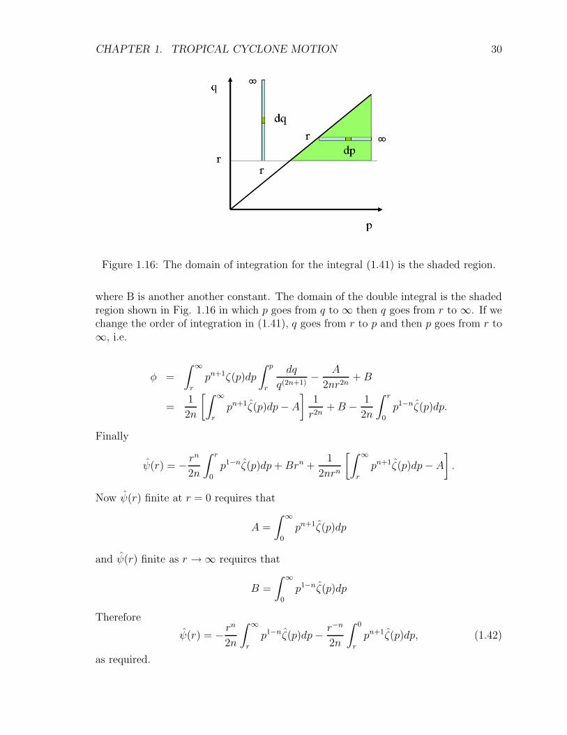
Figure 1.16: The domain of integration for the integral (1.41) is the shaded region.

where B is another another constant. The domain of the double integral is the shadedregion shown in Fig. 1.16 in which p goes from q to ∞ then q goes from r to ∞. If wechange the order of integration in (1.41), q goes from r to p and then p goes from r to∞, i.e.

φ =

∫ ∞

r

pn+1ζ(p)dp

∫ p

r

dq

q(2n+1)− A

2nr2n+B

=1

2n

[∫ ∞

r

pn+1ζ̂(p)dp− A

]1

r2n+B − 1

2n

∫ r

0

p1−nζ̂(p)dp.

Finally

ψ̂(r) = − rn

2n

∫ r

0

p1−nζ̂(p)dp+ Brn +1

2nrn

[∫ ∞

r

pn+1ζ̂(p)dp− A

].

Now ψ̂(r) finite at r = 0 requires that

A =

∫ ∞

0

pn+1ζ̂(p)dp

and ψ̂(r) finite as r → ∞ requires that

B =

∫ ∞

0

p1−nζ̂(p)dp

Therefore

ψ̂(r) = − rn

2n

∫ ∞

r

p1−nζ̂(p)dp− r−n

2n

∫ 0

r

pn+1ζ̂(p)dp, (1.42)

as required.


1.6.2 Solution of Eq. 1.25

The asymmetric flow Ua is obtained from Eqs. (1.17) and (1.18) and c is obtainedfrom (1.21). We can calculate the streamfunction Ψ′

a of the vortex-relative flow Ua−c,from

ψ′n = ψa − ψc,

where

ψ′c = r(Va cos λ− Ua sinλ) = r

[∂Ψ1

∂r

∣∣∣∣r=0

cosλ+∂Ψ2

∂r

∣∣∣∣r=0

sin λ

]. (1.43)

Then using (1.15), (1.16), (1.20) and (1.43) we obtain

ψ′a = Ψ′

1(r, t) cos θ + Ψ′2(r, t) sin θ, (1.44)

where

Ψ′n(r, t) = Ψn − r

[∂Ψn

∂r

]r=0

, (n = 1, 2)

=1

2r

∫ r

0

(1 − p2

r2

)ζn(p, t)dp. (1.45)

After a little more algebra it follows using (1.17), (1.18), (1.21) and (1.45) that

−(Ua − c) · ∇ζs = χ1(r, t) cosλ+ χ2(r, t) sin λ, (1.46)

where [χ1(r, t)χ2(r, t)

]=

1

r

dζsdr

×[ψ′

2(r, t)−ψ′

1(r, t)

]. (1.47)

Now using (1.46) and (1.47), Eq. (1.45) can be written as

dζa1

dT=

1

r

dζsdr

(Ψ′2(r, t) cosλ− Ψ′

1(r, t) sinλ) ,

where d/dt denotes integration following a fluid parcel moving in a circular path ofradius r about the vortex centre with angular velocity Ω(r). It follows that

ζa1 =1

r

dζsdr

∫ t

0

[Ψ′2(r, t

′) cosλ(t′) − Ψ′1(r, t

′) sinλ(t′)]dt′,

where λ(t′) = λ− Ω(r)(t− t′). Using Eq. (1.45), this expression becomes

ζa1 =1

2

dζsdr

∫ t

0

∫ r

0

(1 − p2

r2

)× [ζ2(p, t

′) cosλ(t′) − ζ1(p, t′) sinλ(t′)] dpdt′,

and it reduces further on substitution for ζn from (1.14) and the above expression forλ(t′) giving

ζa1 =1

2βdζsdr

∫ r

0

p

(1 − p2

r2

)

×∫ t

0

[cos {λ− Ω(r)(t− t′)} − cos {λ− Ω(r)(t− t′) − Ω(p)t′}]dt′dp.


On integration with respect to t′ we obtain

ζa1(r, θ, t) = ζ11(r, t) cosλ+ ζ12(r, t) sinλ (1.48)

where

ζ1n(r, t) =

∫ t

0

χn(r, t)dt

= −1

2βdζsdr

∫ r

0

p

(1 − p2

r2

)ηn(r, p, t)dp, (1.49)

and

η1(r, p, t) =sin {Ω(r)t}

Ω(r)− sin {Ω(r)t} − sin {Ω(p)t}

Ω(r) − Ω(p), (1.50)

η2(r, p, t) =1 − cos {Ω(r)t}

Ω(r)+

cos {Ω(r)t} − cos {Ω(p)t}Ω(r) − Ω(p)

, (1.51)

The integrals in (1.50) can be readily evaluated using quadrature.

Documents

1.2 Vorticity-streamfunction method - uni-muenchen.deroger/Lectures/Tropical... · 1.2 Vorticity-streamfunction method The vorticity-streamfunction method is a powerful way of solving