TRANSPORTATION RESEARCH RECORD 1216 29
A Simplified Pavement Maintenance Cost Model
SAMEH M. ZAGHLOUL, EssAM A. SHARAF, AND AHMED A. GADALLAH
This paper presents a summary of an effort to develop a simplified pavement maintenance cost model for the Roads and Bridges Authority (RBA) of Egypt. The model was based primarily on modeling maintenance costs as a function of pavement condition. The study site included the highway network of the East-Delta district as well as several individual highways in the Delta region. The data collected for this study included information on pavement condition in terms of distress type and class. Pavement condition data were obtained from a previous large- cale ludy conducted in Egypt. Maintenance pra ·tices and unit costs were obtained from RBA's fiJes, as well as from extensive interviews with experts from highway construction com1>anies. The results indicated a significant sensitivity of maintenance costs to pavement condition at a certain condition range. It was determined that substantial savings in maintenance costs can be obtained by keeping pavement condition from reaching this condition range or at least by prolonging the period before this range is reached. In addition, it was recommended that the presence of such maintenance cost models can draw the attention of top management, particularly in developing countries, to the importance of the systematic monitoring of pavement condition as well as to the fact that maintenance budget allocation should not always follow the rule of "the worst is first."
Pavement maintenance management (PMM) is the process of coordinating and controlling a comprehensive set of activities to maintain pavements. Simply stated, it enables the best use of available resources by minimizing costs and maximizing benefits (1).
A successful PMM scheme should include a maintenance cost model that is sensitive and responsive to pavement condition. Reliable cost estimates can then be obtained based on actual factors affecting pavement condition (such as materials, design, quality control, and policies).
In some U.S. highway departments and in Egypt, as well as in several other developing countries, pavement maintenance cost estimates are often based primarily on previous experience. This usually leads to a wide gap between the estimates and actual project costs. It is believed that the use of a successful cost model can reduce this gap. A cost model can quantify the consequences of different pavement maintenance activities. In addition, it can specify those condition regions at which pavement maintenance costs are most sensitive to pavement condition. Policies can be set to keep pavements from reaching these critical regions or at least to prolong the period before they are reached.
This study was initiated to develop a simplified pavement
Public Works Department, Cairo University, Giza, Egypt.
maintenance cost model to be. used by the Egyptian Roads and Bridges Authority (RBA) in the development of a Maintenance Management System (MMS). The model presented in this paper employs condition data (represented by the most common method of pavement evaluation-pavement surface condition assessment) and detailed costing of different maintenance activities and practices.
DEVELOPMENT OF MAINTENANCE COST MODEL
Purpose of Model
The main purpose of the maintenance cost model is to determine the costs required to restore pavement surface condition to its "as-constructed state" for various levels of serviceability. This information is important as feedback for planning, design, and construction. The type and degree of maintenance can influence the rate of serviceability loss of pavement. The maintenance cost model can help pavement managers plan, direct, and control maintenance activities so an acceptable level of service, consistent with the class of pavement, can be achieved. In addition, it can assist in evaluating the methods and materials used in maintenance so that efficient, economical practices can be developed.
Network and Section Identification
The network considered in the development of this model included all paved highways in the East-Delta District as well as a set of individual highways representing different areas of the overall Delta paved network. The network length was 1592 km, of which 1547 km were managed by RBA and 45 km by the Ministry of Reconstruction. The network was divided into 327 homogeneous sections on the basis of the following factors:
• Pavement types and age, • Layer types and thicknesses, • Traffic volumes, • Geometric characteristics (such as number of lanes, lane
width, and shoulders), and • Highway class.
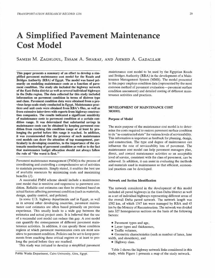
Table 1 shows the highway network links considered in this study, while Figure 1 presents a map of the study network.
30 TRANSPORTATION RESEARCH RECORD 1216
TABLE 1 HIGHWAY NETWORK LINKS
Highway Name Length Authority District Name (km)
Cairo-Alex. 204 x 2 RBA 14611.m c. Delta Dis. (Agriculture) (2-Wa y) , 26km 11 . Delta Dis.
20011.m w. Delta Dis.
Cairo-Alex 205 RBA 90.5km c. Delta Dis. (Desert) 114.5kmW. Delta Dis.
Cairo-Ism. 96 RBA 34.0km c. Delta Dis (Desert) 64.0km I. Delta Dis
Cairo-Suez 116 RBA 40km c. Delta Dis. 76km I. Delta Dis.
Bnha-11ansoura , 49 RBA East-Delta Damietta
Damietta-Dibh 45 Ministry of ---------Reconstruction
Dibh-Port Said 16
eanha-Zagaz ig - 106 Sa I eh i a
Hawata-Sherbin- 79 Blqas
Talkha-Sherbin- 90 Damietta
Abu Hammad-Zagazig 53 -11 it Ghamr
Belbis-11ansoura 75
Abu Kebir-Senbe 26 11 awen
Dekerness-11ansoura 26
raqous-Hessenia 25
Talkha-etqas 16
Es bt Ba ta - 49 Daher i a
Total=1592
Condition Data
The data included in this study were based on a condition survey conducted in the Delta Study (2) in 1981. In this study, the most common distress types in Egypt were found to be
• Crackmg (longitudinai, transverse, map 1.:1a1.:ks), • Surface damage (holes, bleeding, crumbling edge), and • Deformations (rutting, unevenness) .
The distress types and their codes are shown in Table 2. The Texas condition survey method (3) was used in the
Delta Study. The original Texas method defined the distress by its type, severity, and den ity. However, in the Delta Study the distress severity and the distress density were combined
RBA East-Delta
RBA East-Delta
RBA East-Delta
RBA East-Delta
RBA East-Delta
RBA East-Delta
RBA East-Delta
RBA East-Delta
RBA East-Delta
RBA East-Delta
RBA East-Delta
and called the distress class (in other words, the distress was defined by its type and class only) . Pavement distress class ranged from 0 lo 3 where 0 meant no distress, 1 meant low density , 2 meant medium density , and 3 meant high density. Table 3 show the percentages of deteriorated areas (densities) corresponding to each distress (type and class) , known
In the research described in this paper, the 327 sections were evaluated separately, and a condition rating index (CRI) was calculated. The CRI followed the survey method used in the Delta Study.
On the basis of professional judgment, the Texas "scores" were modified as shown in Table 4. The RI can be calculated by summing the score for each distress (in the same section) and determining a general rating for the section (see Table
Zaghlou/ et al.
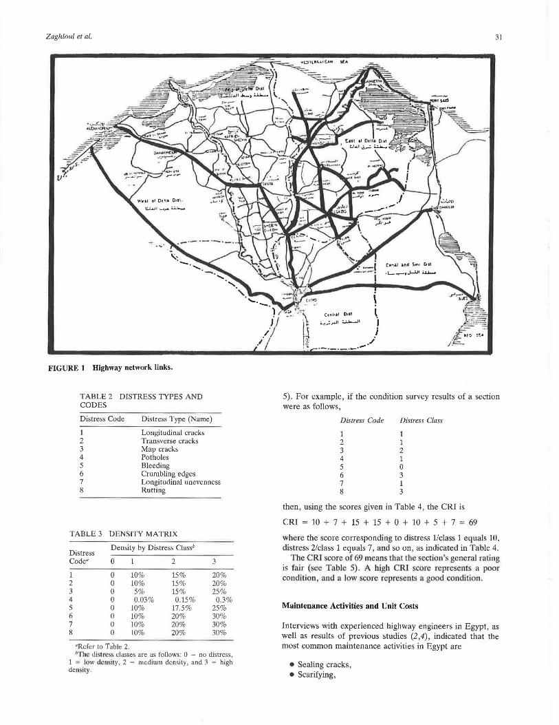
FIGURE 1 Highway network links.
TABLE 2 DISTRESS TYPES AND CODES
Distress Code Distress Type (Name)
Longitudinal cracks Transverse cracks Map cracks Potholes Bleeding
1 2 3 4 5 6 7 8
Crumbling edges Longitudinal unevenness Rutting
TABLE 3 DENSITY MATRIX
Distress Density by Distress Classh
Code" 0 2 3
1 0 10% 15% 20% 2 0 10% 15% 20% 3 0 5% 15% 25% 4 0 0.03% 0.15 % 0.3 % 5 0 10% 17.5% 25% 6 0 10% 20% 30% 7 0 10% 20% 30% 8 0 10% 20% 30%
•Refer to Table 2. "!'he di trc s classes are as follows: 0 = no distress,
1 = low density, 2 = medium density, and 3 = high density.
....... -. ) '.'.".. ' .. \ Y ., ..
/ j
("'11111 0·•' 4-:"_,.!,.JI :.;..a......JI
\ l I i
31
I 1-1.-. I ·~ --·-·- .. -·-- .. i
5). For example, if the condition survey results of a section were as follows,
Distress Code
1 2 3 4 5 6 7 8
Distress Class
1 1 2 1 0 3 1 3
then, using the scores given in Table 4, the CRI is
CRI = 10 + 7 + 15 + 15 + 0 + 10 + 5 + 7 = 69
where the score corresponding to distress l/class 1 equals 10, distress 2/class 1 equals 7, and so on, as indicated in Table 4.
The CRT core of 69 means that the section's gencraJ rating is fair ( ee Table 5). A high CRI core represent a poor condition and a low score represent a good condition.
Maintenance Activities and Unit Costs
Interviews with experienced highway engineers in Egypt, as well as results of previous studies (2,4), indicated that the most common maintenance activities in Egypt are
• Sealing cracks, • Scarifying,
32
TABLE 4 WEIGHTING FACTORS FOR DIFFERENT DISTRESS TYPES
Distress Code"
1 2 3 4 5 6 7 8
Modified Score by Distress Classb
0
0 0 0 0 0 0 0 0
10 7
10 15 2 5 5 2
2
15 12 15 20 5 7 7 5
"Refer to Table 2.
3
20 15 25 25 7
10 10 7
bThe distress classes are as follows: 0 = no distress, 1 = low density, 2 = medium density, and 3 = high density .
TABLE 5 SECTION RATINGS
CRI Section Class
s30 Very good 30-60 Good 60-70 Fair 70-85 Poor 2:85 Very poor
TABLE 6 AVAILABLE MAINTENANCE ACTIVITIES
Maintenance Activity Code
Xl X2 X3 X4
X5 X6
X7 XS
• Seal coating, • Skin patching, • Deep patching, and
Maintenance Activity Name
Sealing cracks Scarifying Seal coating Skin patching without applying
wearing surface Skin patching Deep patching without
applying wearing surface Deep patching Overlay
• Overlaying (see Table 6).
Unit cost computation approaches for each of these activities are briefly described in the following sections.
Sealing Cracks
Cracks Less Than 3 mm in Width The common practice is to fill cracks less than 3 mm wide with a rapid-curing cutback liquid asphalt (RC-5) or with an asphalt cement (60/70 or 80/100 penetration grades). The rate of application used is approximately 0.25 kg/m2 •
TRANSPORTATION RESEARCH RECORD 1216
Cracks Wider Than 3 mm Two methods are commonly used for cracks wider than 3 mm. In the first method, a liquid asphalt or an asphalt cement is applied, then clean sand is spread over the cracked area. The second method uses a sand mix to fill the cracks. The unit cost calculation for this activity is based on an average condition; therefore , the cost is calculated for an application of 0.25 kg/m2 of asphalt cement and 0.5 cm of clean sand.
Scarifying
Scarifying is defined as spreading a fine aggregate (sand) during hot weather and then scarifying this aggregate using a scraper. The cost calculation is based on the cost of spreading the sand (at an average depth of 2 cm) and the cost of scarifying the sand.
Seal Coating (Surface Dressing)
Two alternatives are given for seal coating:
1. Sand coat (1 cm sand + 1.5 kg/m2 of liquid asphalt), and
2. Seal coat (1 cm crushed stone + 1.5 kg/m2) of liquid asphalt.
Skin Patching
Skin patching is defined as removing the top 5 cm of the deteriorated surface and replacing it with a new asphalt concrete surface mix. Cost calculations are based on three items:
1. Cost of removing, loading, and transporting the top 5 cm of the old surface,
2. Cost of tack coating the vertical sides of the cut with asphalt (0.5 kg/m2), and
3. Cost of securing, placing, and compacting the new asphalt concrete surface mix.
Deep Patching
In Egypt, deep patching is defined as the removal of the full pavement depth (surface, binder, base course layers, and 15 cm of the upper portion of the subgrade) and the placement of new courses. Cost items include the following:
• Cost of removing, loading, and transporting the full depth of pavement (approximately 45 cm thick),
• Cost of tack coating the vertical sides of the cut with asphalt (0.5 kg/m2),
~ Cc~! cf seC!!!i~g, p!9.cing, !l!!d romrrnr.tine 20 cm of pitrun gravel as a base course,
• Cost of prime coating the base course surface with a liquid asphalt (1.5 kg/m2),
• Cost of securing, placing, and compacting 5 cm of an asphalt concrete binder course mix,
• Cost of tack coating the binder course surface with a liquid asphalt (0.5 kg/m2), and
• Cost of securing, placing, and compacting 5 cm of an asphalt concrete surface course mix.
Zaghloul et al.
I. ~. Oreok1 z_ Tr111 .. oraek1 I. M1p Craok1 4- itotholH e- llH ding e .. cr..elilg Edge T • L.Ht.UNftMt l·lhlttlng
Malnttnonot Act Iv itJ Matri1
Maintenance Analy1l1 Matria
If T ht re Is Ovtrla y No Scarifying
_ Crack Stolingin1ttd of Stal Cooting
- No Wtorlno Surface In Skin or Dttp P atchlno
- 0 verlaJ over Th• a II Section
M o 1 t ColMltn Dl1trt11 (Type ~:::::::jJ)t ondC1011)ln"' naity M•trix Egrpt II Otter. 111intd
Ava ilob4t Moinie. nonce Actlvltltl In Egypt i 1 Deter. lftlntd and Their Unit Co 1t1
Row ~======::::::! Co nd.
it ion
Sultablt Mainte. nonce Actlvltiu are Sugg11ttd
__ ,......., For Elle h Di1tr. tll (TJpt &Clo
Check thl Over-
lap Condi t ion•
Required Maint Cott ( L.E I "'2)
Data
Condition Progra111
c1e/ ~CRI
33
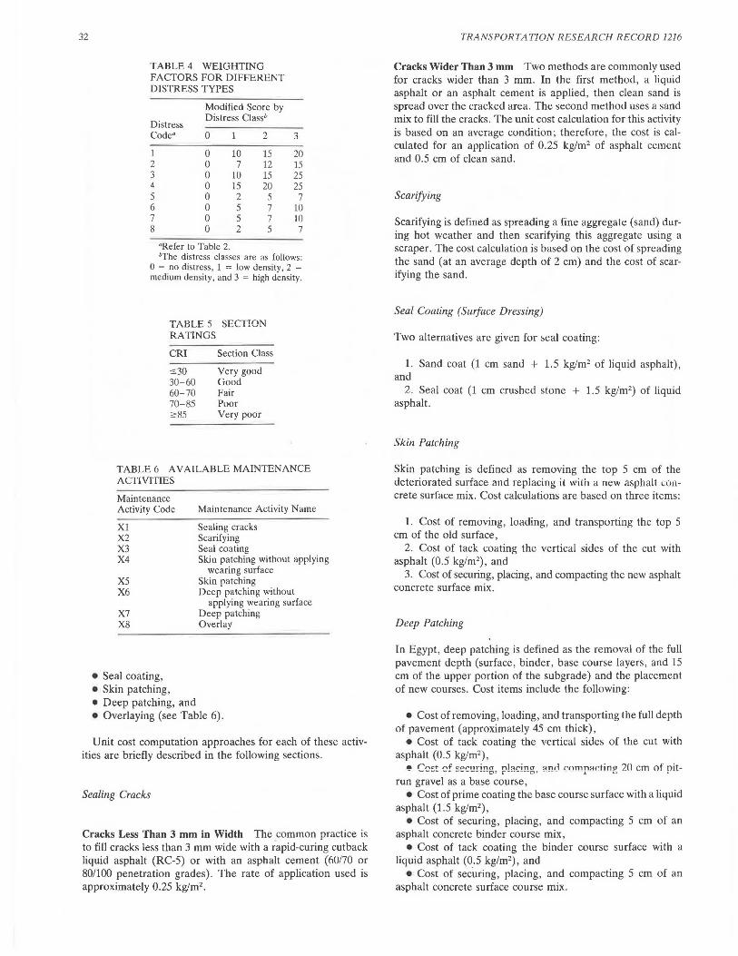
Scor11
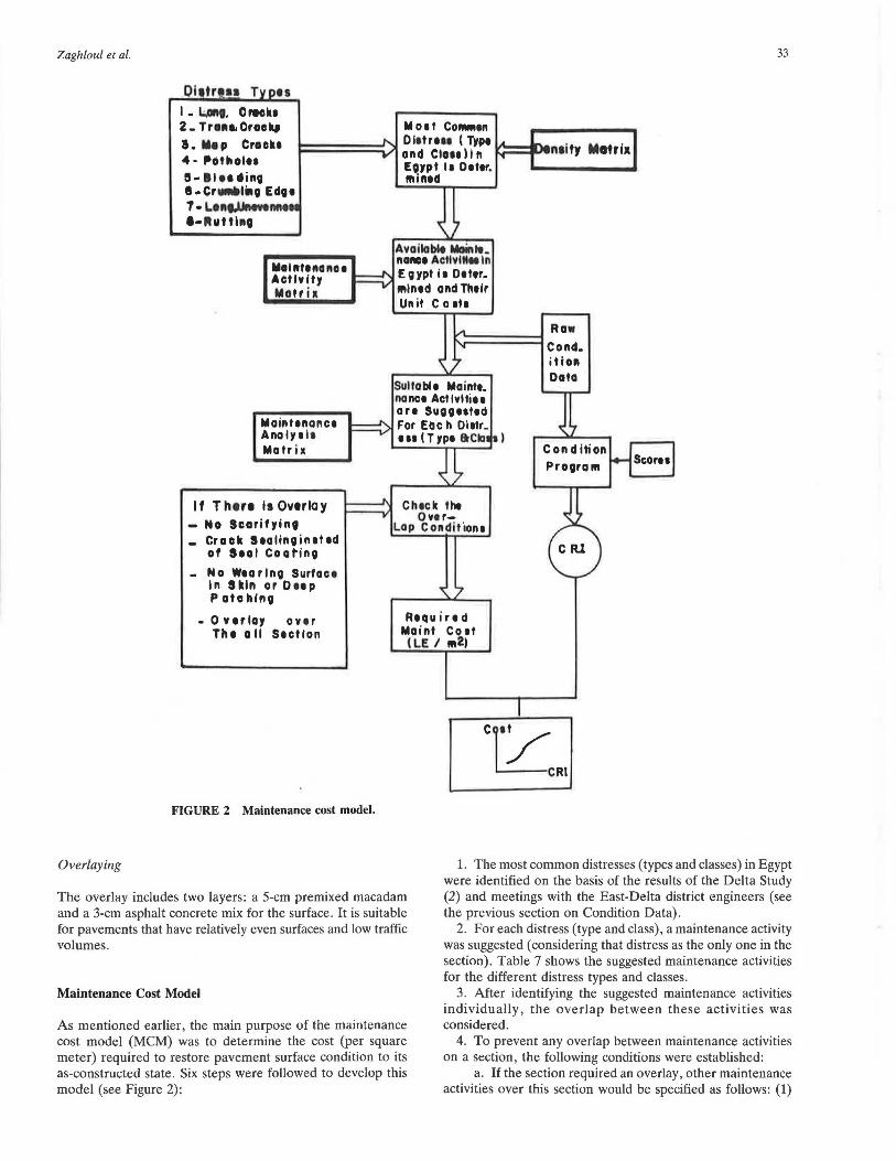
FIGURE 2 Maintenance cost model.
Overlaying
The overlay includes two layers: a 5-cm premixed macadam and a 3-cm asphalt concrete mix for the surface. It is suitable for pavements that have relatively even surfaces and low traffic volumes.
Maintenance Cost Model
As mentioned earlier, the main purpose of the maintenance cost model (MCM) was to determine the cost (per square meter) required to restore pavement surface condition to its as-constructed state. Six steps were followed to develop this model (see Figure 2):
1. The most common distresses (types and classes) in Egypt were identified on the basis of the results of the Delta Study (2) and meetings with the East-Delta district engineers (see the previous section on Condition Data) .
2. For each distress (type and class), a maintenance activity was suggested (considering that distress as the only one in the section). Table 7 shows the suggested maintenance activities for the different distress types and classes.
3. After identifying the suggested maintenance activities individually, the overlap between these activities was considered.
4. To prevent any overlap between maintenance activities on a section, the following conditions were established:
a. If the section required an overlay, other maintenance activities over this section would be specified as follows: (1)
34
TABLE 7 SUGGESTED MAINTENANCE ACTIVITIES FOR EACH DISTRESS (TYPE AND CLASS)
Maintenance Activity Code by
Distress Distress Classb
Code" 0 2 3
1 None Xl Xl X3 2 None Xl Xl X3 3 None XS XS XS 4 None X7 X7 X7 s None None X2 X2 6 None None XS XS 7 None XS XS XS 8 None None XS XS
"Refer lo Table 2. "The distress classes arc as follows: 0 = no
distress , 1 = low density , 2 = medium density, and 3 = high density.
TABLE 8 MAINTENANCE ACTIVITY UNIT COSTS
Maintenance Activity Code"
Xl X2 X3 X4 XS X6 X7 X8
"Refer to Table 6.
Maintenance Activity Cost (£E/m2
)
0.18 0.20 0.92 l.lS S.30 7.50
22.SO 6.90
no scarifying would be conducted; (2) sealing cracks would replace seal coating; and (3) skin or deep patching would be applied without a wearing surface.
b. The overlay would be carried over the entire section (density equals 1.0).
The mathematical representation of these conditions is as follows:
If there is X8, then
X2 = 0
X3 = Xl
X5 X4
X7 X6
D8 = 1.0
5. Tht: maimt:nanct: adivity cusis (Egyptian puumi £Eim~) were obtained from the East-Delta district files and were verified by the Arab Contractors Company engineers. Table 8 shows the unit cost (£E/m2) associated with the different maintenance activities.
6. The section maintenance cost (£E/m2) was then calculated as follows:
TRANSPORTATION RESEARCH RECORD 1216
where
Cr = total unit cost (£E/m2) of the entire section,
D; density of the ith distress type class (from Table 3), and
c, maintenance unit cost corresponding to the ith distress type class (from Table 8).
Application of the MCM
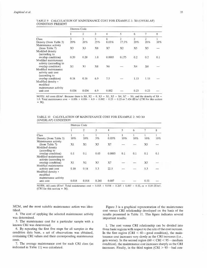
The application of the MCM can be best illustrated through examples. The two examples provided below include actual condition cases. In each example, the distress data (type and class) are presented first. The steps described above are applied in a systematic manner to determine the section maintenance unit cost.
Example 1, Highway 5, Station 38.6
Distress Code
1 2 3 4 s 6 7 8
Distress Class
3 3 3 1 2 2 2 1
The maintenance cost was calculated as in Table 9. Because there was an X8 maintenance activity code , X2 = 0, X3 = Xl, X5 = X4, and X7 = X6, and the density of X8 = 1.0 (overlap condition).
Example 2, Highway 50, Station 159
The distress class was 1 for all distress codes. The maintenance cost was calculated as shown in Table 10. There was no X8 maintenance activity code (overlap condition) .
RELATIONSHIP BETWEEN PAVEMENT CONDITION AND MAINTENANCE COST
Although a pavement condition rating can provide the decision maker with a clear picture of how the network is behaving, it does not indicate how much it will cost to repair the network . Without a clear model of the relationship between pavement condition and repair cost, the ultimate goal of pavement condition assessment cannot be achieved.
The purpose of this study, therefore, was to develop the n >:IMinnship hP.tWP.P.n the CRT and the corresoondin!! reoair and maintenance cost based on the MCM. Th~ following procedure was used to develop this relationship:
1. Each of the samples stored in the condition data base was considered.
2. The existing distresses and their corresponding classes were identified, and the CRI was calculated.
3. The identified distresses were processed through the
Zaghloul et al. 3S
TABLE 9 CALCULATION OF MAINTENANCE COST FOR EXAMPLE 1: XS (OVERLAP) CONDITION PRESENT
Distress Code
2 3 4 s 6 7 s Class 3 3 3 1 2 2 2 1 Density (from Table 3) 20% 20% 2S% 0.03 % 17.S% 20% 20% 10% Maintenance activity
(from Table 7) X3 X3 XS X7 X2 XS XS Modified density
(according to overlap condition) 0.20 0.20 1.0 0.0003 0.17S 0.2 0.2 0.1
Modified maintenance activity (according to overlap condition) Xl Xl XS X6 X4 X4
Modified maintenance activity unit cost (according to overlap condition) O.lS O.lS 6.9 7.S l.lS l.lS
Modified density • modified maintenance activity unit cost 0.036 0.036 6.9 0.002 0.23 0.23
NOTE: All costs £Elm2. Because there is XB, X2 = 0, X3 = Xl , XS = X4, X7 = X6, and the density of X8 =
1.0. Total maintenance cost = 0.036 + 0.036 + 6.9 + 0.002 + 0.23 + 0.23 or 7.434 £Elm2 (CRI for this section = 96).
TABLE 10 CALCULATION OF MAINTENANCE COST FOR EXAMPLE 2: NO XS (OVERLAP) CONDITION
Distress Code
2 3 4 s 6 7 s Class 1 1 1 l 1 1 1 Density (from Table 3) 10% 10% S% 0.03 % 10% 10% 10% 10% Maintenance activity
(from Table 7) Xl Xl XS X7 XS Modified density
(according to overlap condition) 0.1 0.1 o.os 0.0003 0.1 0.1 0.1 0.1
Modified maintenance activity (according to overlap condition) Xl Xl XS X7 XS
Modified maintenance activity unit cost O.lS O.lS S.3 22 .S S.3
Modified density • modified maintenance activity unit cost O.DlS O.Dl S 0.26S 0.007 O.S3
NOTE: All costs £Elm2 • Total maintenance cost = 0.018 + 0.018 + 0.265 + 0.007 + 0.53, or = 0.84 £Elm2•
( CRI for this section = S6).
MCM, and the most suitable maintenance action was identified.
4. The cost of applying the selected maintenance activity was determined.
5. The maintenance cost for a particular sample with a known CRI was determined.
6. By repeating the first five steps for all samples in the condition data base, a set of observations was obtained, containing CRI values and their corresponding maintenance costs .
7. The average maintenance cost for each CRI class (as indicated in Table 11) was calculated.
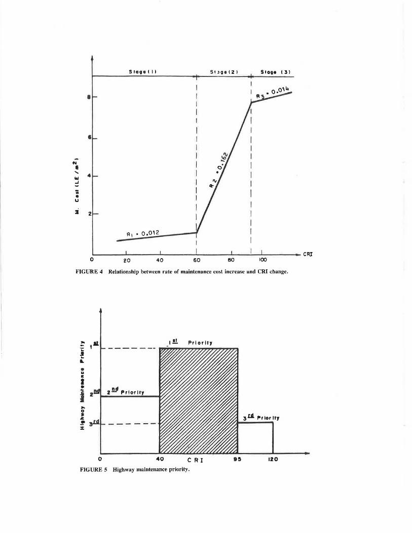
Figure 3 is a graphical representation of the maintenance cost versus CRI relationship developed on the basis of the results presented in Table 11. This figure indicates several important results:
1. The cost versus CRI relationship can be divided into three basic regions with respect to the rate of the cost increase. In the first region (CRI < 60-good condition), the maintenance cost increases very slowly as the CRI increases (i.e. , gets worse) . In the second region (60 < CRI < 95-medium condition), the maintenance cost increases sharply as the CRI increases. Finally, in the third region (CRI > 95-bad con-
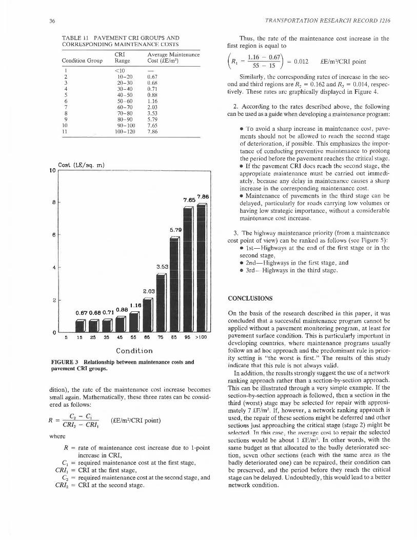
36
TABLE 11 PAVEMENT CRI GROUPS AND CORRESPONDING MAINTENANCE COSTS
Condition Group
1 2 3 4 5 6 7 8 9
10 11
Cosl (LE/sq. m)
CRI Range
< 10 10-20 20-30 30-40 40-50 50-60 60-70 70-80 80-90 90-100
100-120
Average Maintenance Cost (£E/m2
)
0.67 0.68 0.71 0.88 1.16 2.03 3.53 5.79 7.65 7.86
10 ,....-~~~~~~~~.~~~~~~~~~~-
8 7 .65 7.86
6
4
2
0 5 15 25 35 45 55 65 75 85 95 >100
Condition
FIGURE 3 Relationship between maintenance costs and pavement CRI groups.
dition), the rate of the maintenance cost increase becomes small again. Mathematically, these three rate.s can be considered as follows:
(£E/m2/CRI point)
where
R = rate of maintenance cost increase due to 1-point increase in CRI,
C1 = required maintenance cost at the first stage, CR/1 = CRI at the first stage,
C2 = required maintenance cost at the second stage, and CR/2 = CRI at the second stage.
TRANSPORTATION RESEARCH RECORD 1216
Thus, the rate of the maintenance cost increase in the first region is equal to
( R = l.lG - 0·67) = 0 012 I 55 - 15 , £E/m2/CRI point
Similarly, the corresponding rates of increase in the second and third regions are R2 = 0.162 and R3 = 0.014, respectively. These rates are graphically displayed in Figure 4.
2. According to the rates described above, the following can be used as a guide when developing a maintenance program:
• To avoid a sharp increase in maintenance cost, pavements should not be allowed to reach the second stage of deterioration, if possible . This emphasizes the importance of conducting preventive maintenance to prolong the period before the pavement reaches the critical stage. • If the pavement CRI does reach the second stage , the appropriate maintenance must be carried out immediately, because any delay in maintenance causes a sharp increase in the corresponding maintenance cost. • Maintenance of pavements in the third stage can be delayed, particularly for roads carrying low volumes or having low strategic importance , without a considerable maintenance cost increase.
3. The highway maintenance priority (from a maintenance cost point of view) can be ranked as follows (see Figure 5):
• 1st-Highways at the end of the first stage or in the second stage, • 2nd-Highways in the first stage, and e 3rd-Highways in the third stage.
CONCLUSIONS
On the basis of the research described in this paper, it was concluded that a successful maintenance program cannot be applied without a pavement monitoring program, at least for pavement surface condition. This is particularly important in developing countries, where maintenance programs usually follow an ad hoc approach and the predominant rule in priority setting is "the worst is first." The results of this study indicate that this rule is not always valid.
In addition, the results strongly suggest the use of a network ranking approach rather than a section-by-section approach. This can be illustrated through a very simple example. If the section-by-section approach is followed, then a section in the third (worst) stage may be selected for repair with approximately 7 £E/m2 • If, however, a network ranking approach is used, the repair of these sections might be deferred and otht!r sections just approaching the critical stage (stage 2) might be sP.lP.rtP.cl Tn this rase, the avernge cost to repair the selected sections would be about 1 £E/m2 • In other words, with the same budget as that allocated to the badly deteriorated section, seven other sections (each with the same area as the badly deteriorated one) can be repaired, their condition can be preserved, and the period before they reach the critical stage can be delayed. Undoubtedly, this would lead to a better network condition.
S IOCJ• t 11 SllOet21 SIOCJ• t 3l
I
I
N E .... ... 4 .J
-• • u
2 2
R1 • 0.012
0 20 40 60 80 100
FIGURE 4 Relationship between rate of maintenance cost increase and CRI change.
,.. ,• I.!!. Priority -...::: ---- ---.I .. L
• u c I • nd
i z 2- Priority
,.. Cl • 3 Lil P"r lor lty .c ~ ~ --- ---
:I:
0 120
FIGURE 5 Highway maintenance priority.

38
REFERENCES
1. Pavement Management Systems. Organization of Economic Cooperation and Development, 1987.
2. Optimum Maintenance Policies for the Delta Paved Road Network . Vol. 1. Development Research and Technological Planning Center, 1981.
3. Texas Transportation Institute and Center of Highway Research.
TRANSPORTATION RESEARCH RECORD 1216
Texas Flexible Pavement System, FPS . Texas Department of Transportation, 1975.
4. Egyptian National Transportation Study, Phase II. Transport Planning Authority, Ministry of Transportation, Cairo, 1981.
Publication of this paper sponsored by Committee on Maintenance and Operations Management.
Recommended