THE JOURNAL OF FINANCE • VOL. LIV, NO. 4 • AUGUST 1999
A Critique of the Stochastic Discount Factor Methodology
RAYMOND KAN and GUOFU ZHOU*
ABSTRACT
In this paper, we point out that the widely used stochastic discount factor (SDF)
methodology ignores a fully specified model for asset returns. As a result, it suffers
from two potential problems when asset returns follow a linear factor model. The
first problem is that the risk premium estimate from the SDF methodology is
unreliable. The second problem is that the specification test under the SDF meth
odology has very low power in detecting misspecified models. Traditional method
ologies typically incorporate a fully specified model for asset returns, and they can
perform substantially better than the SDF methodology.
AssET PRICING THEORIES, such as those of Sharpe (1964), Lintner (1965), Black (1972), Merton (1973), Ross (1976) , and Breeden (1979) , show that the expected return on a financial asset is a linear function of its covariances (or betas) with some systematic risk factors . This implication has been tested extensively in the finance literature by the so-called "traditional methodologies." In the traditional methodologies, a data-generating process is first proposed for the returns, and then the restrictions imposed by an asset pricing model are tested as parametric constraints on the return-generating process . The approach taken by the traditional methodologies has a potential problem, which is that when the proposed return-generating process is misspecified the test results could be misleading. Therefore, in applying the traditional methodologies, researchers typically have to justify that the proposed data-generating process provides a good description of the returns . For example, when the proposed return-generating process is a factor model, one would like the model to have high R2 in explaining the returns on the test assets , especially when the test assets are well-diversified portfolios.
As many of the earlier theories are special cases of the stochastic discount factor (SDF) model, recent empirical asset pricing studies have been focused on testing the pricing restrictions in terms of the SDF model, rather
*Kan is from the University of Toronto, Zhou is from Washington University in St. Louis. We
thank Kerry Back, Philip Dybvig, Heber Farnsworth, Wayne Ferson, Campbell Harvey, Roger
Huang, Ravi Jagannathan, Mark Loewenstein, Deborah Lucas, Akhtar Siddique, Hans Stoll,
Zhenyu Wang, Chu Zhang, seminar participants at the National Central University of Taiwan,
the University of Texas at Dallas, Washington University in St. Louis, and participants at the
1999 American Finance Association Meetings in New York for their helpful discussions and comments. Kan gratefully acknowledges financial support from the Social Sciences and Hu
manities Research Council of Canada.
1221
1222 The Journal of Finance
than on the traditional risk measures such as the beta and the Sharpe ratio. One of the most prominent papers in this line of research is Cochrane (1996) , where the SDF methodology is fully explained. The formulation typically estimates the parameters and tests the pricing implications without a fully specified model of how the asset retums are generated in the economy. On the one hand, this appears very general and requires fewer assumptions and parameters than the traditional methodologies . On the other hand, it seems counterintuitive that one can be sure the pricing restrictions are true even if one knows little about the dynamics of the returns-that is, without a fully specified model (either parametric or nonparametric) of the returns.
This paper shows that if asset returns are generated by a linear factor model, then by ignoring the full dynamics of asset returns , as is currently done in empirical studies using the SDF methodology, two potential problems arise. The first problem is that the accuracy of the parameter estimation can be poor: the standard error of the estimated risk premium is often more than 40 times greater than that of the traditional methodologies, which should make one extra cautious when applying the SDF methodology. The second problem with the SDF methodology is that its specification test has very low power against misspecified models . With the usual sample size that we encounter in empirical studies , our simulation evidence suggests that the SDF methodology is not very reliable in detecting even gross misspecifications in an asset pricing model, especially when the proposed factors are not highly correlated with the retums.
The rest of the paper is organized as follows . The next section presents the traditional beta pricing model and the SDF model , and the empirical methodologies that are typically used to estimate and test such models. Though these are standard in the literature, the purpose here is to introduce notations and to facilitate later discussions . We also provide the intuition why the SDF methodology may not perform well when there is a lack of a fully specified model for the asset returns . In Sections II and III, we use asymptotic theory and Monte Carlo simulations to compare the performance of the traditional and SDF methodologies. The conclusions are in the final section.
I. Traditional and SDF Methodologies
A. Tests of the Traditional Beta Pricing Model
In order to make the results more easily understood, we present them in the simplest form. Let rt be the excess retum (in excess of the risk-free rate) on N risky assets at timet. Traditional methodologies begin by proposing a retum-generating process for the excess returns, typically one that provides good explanatory power on the excess returns. For example, one may propose that excess retums are generated by a one-factor model
rt = a + f:Jft + Bt' (1)
A Critique of the Stochastic Discount Factor Methodology 1223
where ft is the realized value of a systematic risk factor at time t, Bt is the idiosyncratic risk of the assets with E[etlfncl»t-d = ON and Var[ s t] = I, where ON is anN-vector of zeros, cl»t_1 is the information set at t - 1, and fJ =
Cov[rn ftlcl»t_ t J/Var[ ftlcl»t_1] is the factor loadings of the returns with respect to the common factor. Since only unexpected shocks matter for unexpected returns, ft can be modeled as a martingale difference sequence; that is, E[ftl4»t_1] = 0. Under these assumptions, a = E[rtlcl»t-d is the expected excess returns on the N assets . In the rest of the paper, the trivial case a = ON is precluded. In general, a and fJ can be functions of information variables at t - 1, but for the purpose of simplifYing technical details and focusing on the main point of this paper, we assume they are constants . Nevertheless, we do not assume Var[ s t I cl»t_1 , ft] = I, so conditional heteroskedasticity in Bt is allowed in our setup.
A beta pricing model, in the exact form, suggests that the expected excess return of an asset is a linear function of its betas with respect to the systematic factors . In our one-factor case, the beta pricing model suggests
a = fJA, (2)
where A is the risk premium. This clearly imposes a testable restriction on the parameters of the return-generating process in equation (1) . Traditional tests of beta pricing model are basically done by carrying out various statistical tests of this restriction.
There are many alternatives to estimate the risk premium A and test the beta pricing model. We describe two representative approaches here . If one is willing to make distributional assumptions on Bt, one can use the maximum likelihood approach. A popular choice is to assume conditional onft, Bt � N(ON,I). Following Zhou (1991, 1995) , we define f = [{1, {2, ... ,fT]', X = [IT,f], Y= [r1 , r2 , ... ,rT]', where T is the number of time series observations, and IT is aT-vector of ones. Let �1::::: �2 > 0 be the two eigenvalues of
A = (X'X)-1(X'Y)(Y'Y)-1(Y'X). (3)
Under the normality assumption, the maximum likelihood estimator of A is given by
(4)
where a;i are the (i,j) th elements of A. The likelihood ratio test (with the Bartlett correction) of equation (2) is1
( N + 3 ) A LRT = - T- -2- log (1- �2) � x�-1,
where � means an asymptotic distribution.
(5)
1 Based on simulation evidence, Zhou (1995) shows that the Bartlett correction can improve
the small sample properties of the likelihood ratio test. The exact small sample distribution of
the likelihood ratio test is also available from Zhou (1991, 1995).
1224 The Journal of Finance
If one does not wish to make any strong distributional assumptions on et , then an alternative approach is to use the generalized method of moments (GMM) of Hansen (1982) to estimate the parameters and test the beta pricing model . Following, for example , MacKinlay and Richardson (1991) or Harvey and Zhou ( 1993) , the GMM test of equation (2) uses the following moment conditions :
To apply the GMM methodology, we define the sample moments as
(8)
where Zt = [ 1.ft ] ' . We assume ft and Bt are jointly stationary and ergodic with finite fourth moments, and under the true parameters ,
(9)
where S1 is a 2N X 2N positive definite constant matrix. This condition is much weaker than those assumed in other methods of testing asset pricing models. It allows for a variety of forms of autocorrelation and heteroskedasticity in zt ® Bt . In the GMM methodology, the estimators of the true parameters A and fJ of the one-factor model, A* and /J*, are given by the solution of the following minimization problem,
( 10)
where W1r is a (possibly stochastic) 2N X 2N positive definite weighting matrix with a limit W that is positive definite and nonstochastic . The standard approach is to choose an optimal weighting matrix equal to a consistent estimate of 811•2 Although there are N + 1 parameters in the beta pricing model and the optimization problem is a nonlinear one, it does not present as a serious problem to the estimation because, conditional on a given value of A, the objective function is linear in fJ and the minimization problem can
2 When the optimal weighting matrix depends on parameters, an iterative method has to be
used. In the first round, a positive definite matrix, say, the identity matrix, is used as the
weighting matrix to estimate the parameters. In the second round, the model is reestimated
using the optimal weighting matrix based on the estimated parameters from the first round.
A Critique of the Stochastic Discount Factor Methodology 1225
be solved analytically. As a result, the estimation problem can be written as a function of..\ alone and a simple line search can be used to find the optimal .A· .a
A test of the traditional beta pricing model a = fJ..\ can be carried out by using Hansen's (1982) overidentification test. Since we have 2N moment conditions and only N + 1 parameters , there are N - 1 overidentification conditions, and hence
(11)
where W1r is a consistent estimate of the optimal weighting matrix.4 However, as Cochrane (1996) and Jagannathan and Wang (1996) suggest, it is sometimes desirable, for good economic reasons, to use a nonoptimal weighting matrix. In this case, J1 will no longer have a simple chi-square distribution, but rather will be a weighted sum of chi-square distributions. Zhou (1994) provides a simple chi-square GMM test for an arbitrary weighting matrix, which can be used to bypass the difficulty of having to calculate a weighted sum of chi-square distributions. A numerically identical test is also proposed by Cochrane (1996) . But an alternative optimal chi-square test can be obtained from the scoring algorithm, as presented by Newey (1985) and analyzed by Zhou (1994) .
B. SDF Model
As discussed by Cochrane (1996) , the beta pricing model is a special case of the SDF model. Under the SDF model, there exists a random variable mt,
the stochastic discount factor, such that
(12)
When the exact one-factor asset pricing model in equation (2) holds, the stochastic discount factor is given by
(13)
for some constants 80 and (\. As an econometric model, the parameters in equation (13) are not uniquely defined. If (80,81) satisfies the equation, so does any multiplier of it. Therefore, it is common to normalize the parameters by writing
(14)
3 Details of the optimization are available upon request. For some special weighting matri
ces, Zhou (1994) even obtains an analytical solution to this optimization problem.
4 Another way of testing a = fJJo. is to estimate a and fJ in equations (6) and (7) as a fully
specified model and test the nonlinear restriction on the parameters using a Wald test.
1226 The Journal of Finance
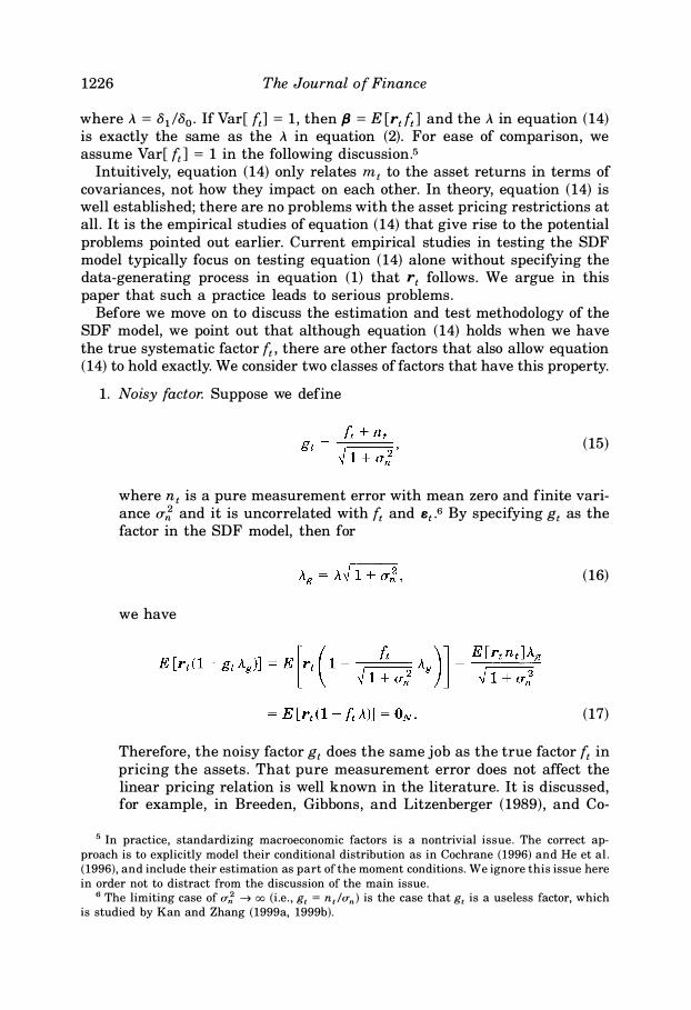
where A = 81 /80. If Var[ ft] = 1, then fJ = E [rt ft] and the A in equation (14) is exactly the same as the A in equation (2). For ease of comparison, we assume Var[ ft ] = 1 in the following discussion.5
Intuitively, equation (14) only relates mt to the asset returns in terms of covariances, not how they impact on each other. In theory, equation (14) is well established; there are no problems with the asset pricing restrictions at all. It is the empirical studies of equation (14) that give rise to the potential problems pointed out earlier. Current empirical studies in testing the SDF model typically focus on testing equation (14) alone without specifying the data-generating process in equation (1) that rt follows. We argue in this paper that such a practice leads to serious problems .
Before we move on to discuss the estimation and test methodology of the SDF model, we point out that although equation (14) holds when we have the true systematic factor ft , there are other factors that also allow equation (14) to hold exactly. We consider two classes of factors that have this property.
1. Noisy factor. Suppose we define
(15)
where nt is a pure measurement error with mean zero and finite variance a; and it is uncorrelated with ft and et .6 By specifying gt as the factor in the SDF model, then for
(16)
we have
(17)
Therefore, the noisy factor gt does the same job as the true factor ft in pricing the assets . That pure measurement error does not affect the linear pricing relation is well known in the literature. It is discussed, for example, in Breeden, Gibbons , and Litzenberger (1989) , and Co-
5 In practice, standardizing macroeconomic factors is a nontrivial issue. The correct ap
proach is to explicitly model their conditional distribution as in Cochrane (1996) and He et al.
(1996), and include their estimation as part of the moment conditions. We ignore this issue here
in order not to distract from the discussion of the main issue. 6 The limiting case of u; � oo (i.e., g, = n,lun ) is the case that g, is a useless factor, which
is studied by Kan and Zhang (1999a, 1999b).
A Critique of the Stochastic Discount Factor Methodology 1227
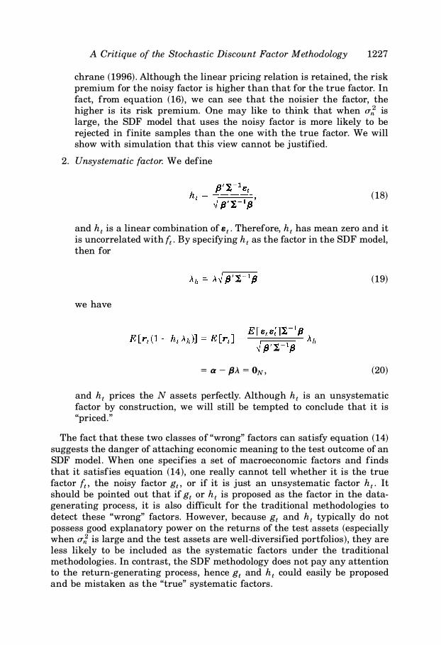
chrane (1996) . Although the linear pricing relation is retained, the risk premium for the noisy factor is higher than that for the true factor. In fact, from equation (16) , we can see that the noisier the factor, the higher is its risk premium. One may like to think that when u; is large, the SDF model that uses the noisy factor is more likely to be rejected in finite samples than the one with the true factor. We will show with simulation that this view cannot be justified.
2. Unsystematic factor. We define
(18)
and ht is a linear combination of Bt. Therefore, ht has mean zero and it is uncorrelated with ft . By specifying ht as the factor in the SDF model, then for
(19)
we have
= a - fJA. = ON, (20)
and ht prices the N assets perfectly. Although ht is an unsystematic factor by construction, we will still be tempted to conclude that it is "priced."
The fact that these two classes of "wrong" factors can satisfy equation (14) suggests the danger of attaching economic meaning to the test outcome of an SDF model . When one specifies a set of macroeconomic factors and finds that it satisfies equation (14), one really cannot tell whether it is the true factor ft , the noisy factor gt, or if it is just an unsystematic factor ht . It should be pointed out that if gt or ht is proposed as the factor in the datagenerating process, it is also difficult for the traditional methodologies to detect these "wrong" factors. However, because gt and ht typically do not possess good explanatory power on the returns of the test assets (especially when u; is large and the test assets are well-diversified portfolios) , they are less likely to be included as the systematic factors under the traditional methodologies . In contrast, the SDF methodology does not pay any attention to the return-generating process , hence gt and ht could easily be proposed and be mistaken as the "true" systematic factors .
1228 The Journal of Finance
Recognizing that there are countless SDFs that represent countless asset pricing models for a given set of asset returns , Hansen and Jagannathan (1991) solve explicitly the SDF that has the minimum variance among all the SDFs. Hansen and Jagannathan (1997) further show how to use SDFs to assess specification errors of asset pricing models. What we have shown here is that there are in fact many SDFs for a given linear factor model. Therefore , explicitly constructed "wrong" factors can potentially help to explain the failure of an asset pricing model. This highlights the danger of using factors in the SDF framework without a careful examination of the explanatory power of the factors.
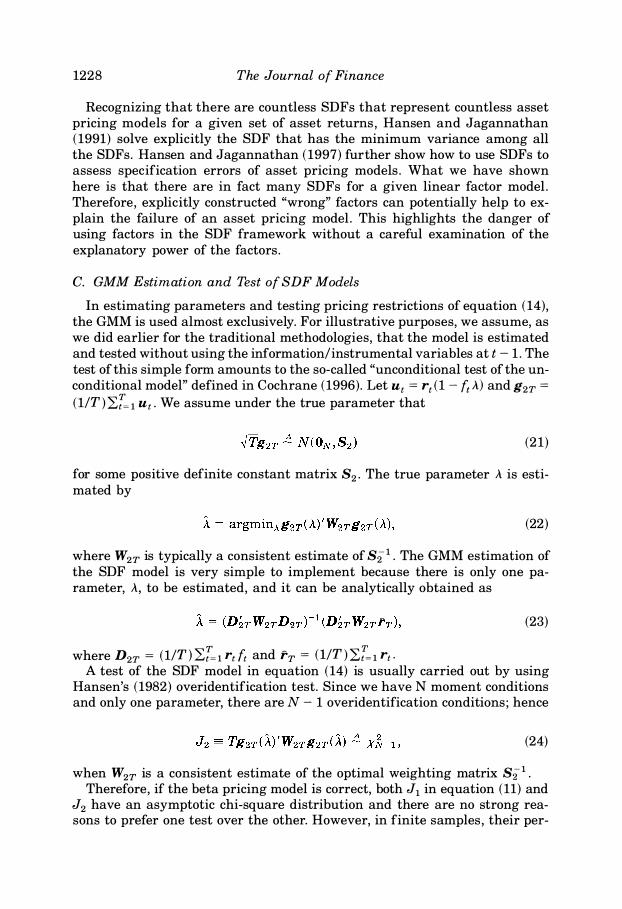
C. GMM Estimation and Test of SDF Models
In estimating parameters and testing pricing restrictions of equation (14), the GMM is used almost exclusively. For illustrative purposes, we assume, as we did earlier for the traditional methodologies, that the model is estimated and tested without using the information/instrumental variables at t - 1. The test of this simple form amounts to the so-called "unconditional test of the unconditional model" defined in Cochrane (1996). Let ut = rt(1- ft A) andg2r =
(1/T)2}�1 Ut. We assume under the true parameter that
(21)
for some positive definite constant matrix 82. The true parameter A is estimated by
(22)
where W2r is typically a consistent estimate of 8:;:1• The GMM estimation of the SDF model is very simple to implement because there is only one parameter, A, to be estimated, and it can be analytically obtained as
(23)
where D2r = (1/T)"'i.[�trdt and i'r = (l!T)'i.'{�lrt. A test of the SDF model in equation (14) is usually carried out by using
Hansen's (1982) overidentification test. Since we have N moment conditions and only one parameter, there are N - 1 overidentification conditions ; hence
(24)
when W2r is a consistent estimate of the optimal weighting matrix 821• Therefore, if the beta pricing model is correct, both J1 in equation (11) and
J2 have an asymptotic chi-square distribution and there are no strong reasons to prefer one test over the other. However, in finite samples , their per-
A Critique of the Stochastic Discount Factor Methodology 1229
formance could differ. More importantly, when the model is misspecified, J1 and J2 could have very different power. We study these issues by simulation in Section III.
Although the estimation problem of the SDF methodology is very simple, ignoring the full dynamics of asset returns introduces serious problems . Intuitively, equation (14) is a restriction on part of the first and second moments between the asset returns and the factor. Testing equation (14) alone without using a fully specified model amounts to ignoring many other first and second moments entirely. As a result, it is not surprising that the estimation error of A can be substantially large . It is also not surprising that a tested factor can be important in equation (14) , but in fact may have little to do with the returns. This is the fundamental reason that causes the problems emphasized by this paper. In the following sections, we provide a comparison of the traditional methodologies with the SDF methodology in terms of the estimation accuracy of risk premium, and in terms of the size and the power of their tests of the asset pricing model .
II. Estimation Accuracy of Risk Premium
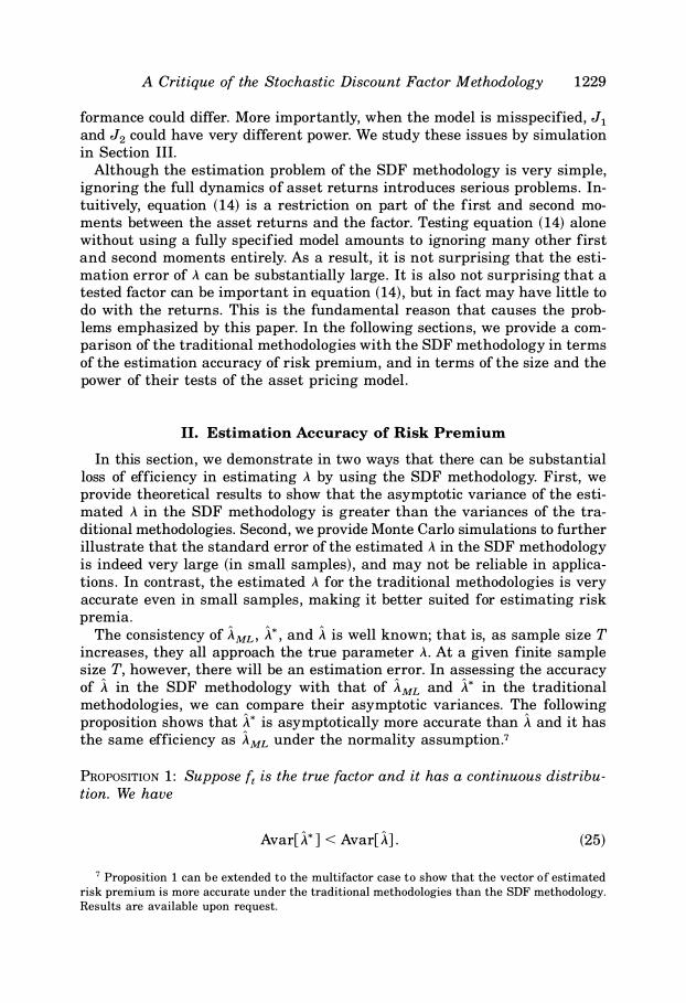
In this section, we demonstrate in two ways that there can be substantial loss of efficiency in estimating A by using the SDF methodology. First, we provide theoretical results to show that the asymptotic variance of the estimated A in the SDF methodology is greater than the variances of the traditional methodologies. Second, we provide Monte Carlo simulations to further illustrate that the standard error of the estimated A in the SDF methodology is indeed very large (in small samples) , and may not be reliable in applications . In contrast, the estimated A for the traditional methodologies is very accurate even in small samples , making it better suited for estimating risk premia.
The consistency of AML• A* , and A is well known; that is, as sample size T increases, they all approach the true parameter A. At a given finite sample size T, however, there will be an estimation error. In assessing the accuracy of A in the SDF methodology with that of AML and A* in the traditional methodologies , we can compare their asymptotic variances. The following proposition shows that A* is asymptotically more accurate than A and it has the same efficiency as AML under the normality assumption.7
PROPOSITION 1: Suppose ft is the true factor and it has a continuous distribution. We have
Avar[ A* ] < Avar[ A] . (25)
7 Proposition 1 can be extended to the multifactor case to show that the vector of estimated
risk premium is more accurate under the traditional methodologies than the SDF methodology.
Results are available upon request.
1230 The Journal of Finance
For the case that Bt has a multivariate normal distribution conditional on ft, we have
(26)
Proposition 1 suggests that regardless of the distribution that Bt follows, with or without conditional heteroskedasticity, traditional methodologies that incorporate the return-generating process will always provide an estimated risk premium that is asymptotically more efficient than that from the SDF methodology. One may like to think that the reason we achieve higher accuracy in A* is that we use more moment conditions than the SDF methodology. However, this is not the main reason for the improvement because, although we do have more moment conditions in the traditional methodology, we also have more parameters to estimate.
There are two main reasons why the full GMM estimator A* in the traditional methodology is more efficient than the SDF estimator A. The first reason is that the full GMM uses jj* to explain average excess returns, whereas the SDF methodology uses D2r = (1/T)2.[=1rtft to explain average excess returns. Both /J* and D2r are consistent estimates of 13 when Var[ ft] = 1; however, in general, /J* is a more accurate estimator of 13 than D2r . For example, under the multivariate normality assumption on ft and Bt, it can be shown that Avar[D2r] = I+ 1313' , which is much larger than
A*
1 [ A21313' ] Avar[ l3 ] = --2 I + ,� 1 < I.8
1+A 13�-13
In the traditional methodology, the moment conditions in equation (7) and the restriction a = I3A allow us to obtain an estimate of 13 with high degree of accuracy. In contrast, the SDF methodology abandons the more accurate beta estimation and only relates the average returns to the average covariances.
The second reason the full GMM estimator A* in the traditional methodology is more efficient than the SDF estimator A is that the realized return is a very noisy measure of expected return. The traditional methodology makes use of the factor structure of the return-generating process by taking away the systematic component 13ft from rt in the moment conditions . When 13ft accounts for a significant portion of the variations of rt, then rt - 13ft is
8 The expression for AvarUJ*] can be obtained from the proof of Proposition 1. The inequality follows because
1 [ A2fJfJ' ] A2 __ I+ __ = I ___ I1;2[I _ I-112fJ(fJ'I-1fJ)-1fJ'I-112]Ill2 1 + A2 fJ'I-1/J 1 + A2 N
and the second term is a positive semidefinite matrix.
A Critique of the Stochastic Discount Factor Methodology 1231
a much less noisy measure of expected return than rt. The SDF methodology, however, does not incorporate the return-generating process in its moment conditions and only relates realized excess returns rt to realized covariance rtf t. When both of these two measures are very noisy, it is not surprising that the SDF methodology does not deliver a very accurate estimate of the risk premium.
The above analysis shows that the traditional methodology, which utilizes the fully specified asset return model, helps to substantially improve the estimation accuracy of A. As a result, it may be tempting to. estimate A by using all of the moment conditions , those of the traditional ones in equations (6) and (7) , and those of the SDF ones in equation ( 14) . It turns out that there is some overlap between these moment conditions. Out of the 3N moment conditions , N - 1 of them are redundant. For example , if we know Bt,
stft , and u lt = rlt( 1 - ft A) where /31 i= 0, then we can obtain the other elements of ut by using the relation
/3i = [rit - /3i (A + ft )] ( 1 - ft A) + - f3t(A + ft ) (1 - ft A)
f3t = rit( 1 - ft A)
= uit , for i = 2 , . . . ,N. (2 7)
Therefore, one can use at most 2N + 1 moment conditions to estimate A. Denote A** and fJ** as the estimator of A and fJ using any 2N + 1 of the combined 3N moment conditions. The following proposition suggests that once the moment conditions in the traditional methodology are used, the additional one from the SDF model does not help to improve the accuracy of the estimation.
PROPOSITION 2: Suppose ft is the true factor. We have
[ A* ] [ A** ] Avar
A = Avar
A •
fJ* fJ** (28)
Note that Proposition 2 does not suggest that any 2N out of the combined 3N moment conditions will do the same job as the traditional methodology. For example , if we combine the N moment conditions in equation (6) (or the N moment conditions in equation (7)) with theN moment conditions in equation ( 14) of the SDF methodology to estimate A, it can be shown that the asymptotic variance of the estimated A using these 2N moment conditions is still the same as that of A from the SDF methodology. Therefore , it is important to choose the proper set of moment conditions to obtain a good estimate of A. Proposition 2 suggests the moment conditions used by the
1232 The Journal of Finance
traditional methodology are the best and they are sufficient to learn almost everything about the parameters . Adding the SDF moment conditions into the traditional ones provides only redundant information.9
Although Proposition 1 suggests that the estimated risk premium in the traditional methodologies is asymptotically more accurate than that of the SDF methodology, it does not tell us the magnitude of improvement, nor does it tell us whether this result holds in finite samples . We address these issues by simulation. The setup of our simulation experiment is as follows. In our simulation, we generate excess returns on 10 assets using a onefactor model. The factor is generated independently from a standard normal distribution and it is designed to capture the behavior of the standardized excess return on the value-weighted market portfolio of the NYSE; that is,
r - E [r ] ft = mt mt
� N(0,1), (29) O"
m
where r mt is the excess return on the market portfolio and O"m is its standard deviation. The betas of the 10 assets are set to equal the sample betas of the 10 size-ranked portfolios of the NYSE with respect to ft, estimated using monthly returns from January 1926 to December 1997. The true risk premium is chosen to make the expected excess returns close to the average excess returns of the 10 size portfolios over the sample period; that is,
A = argmin .. (i• - /3A) ' (r - /3A) , (30)
where r and f3 are the average returns and sample betas of the 10 sizeranked portfolios. Finally, the model disturbances are independently generated from a multivariate normal distribution
(31)
where I is chosen to be the sample covariance matrix of the market model residuals of the 10 size-ranked portfolios . In Table I, Panel A, we present the parameters a, /3, and A of the 10 assets we use in our simulation. Note that the value we choose for A (0.1373) is very close to the sample Sharpe ratio for the value-weighted market portfolio of the NYSE, which is equal to 0.1248 for the period January 1926 to December 1997.10
We generate returns from this one-factor model for different lengths of time series and apply the traditional and the SDF methodologies to estimate the risk premium A. In Panel B of Table I, we present a summary of the
9 Similar to Proposition 1, Proposition 2 continues to hold for the multifactor case. When there are k-factors, only k of the SDF moment conditions can be added to the traditional moment conditions, and they do not improve the estimation accuracy of the risk premium and the betas. Results are available upon request.
10 Under our definition of{,, A is equal to the Sharpe ratio of the market portfolio if the CAPM holds.
A Critique of the Stochastic Discount Factor Methodology 1233
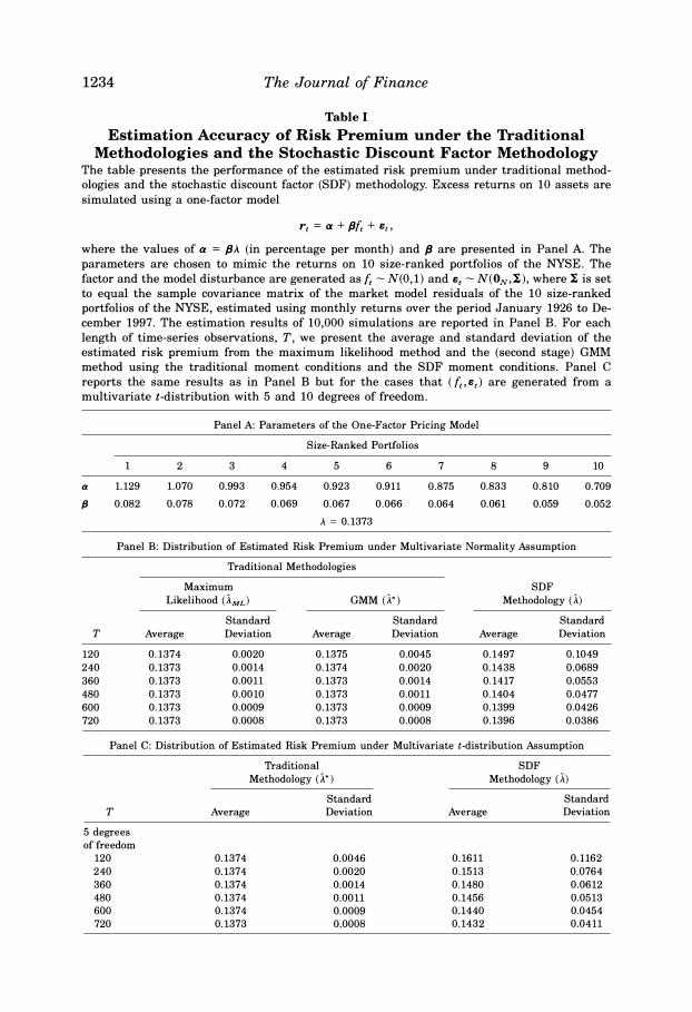
estimation results in 10,000 simulations . For the traditional methodologies , we report the average and standard deviation of the estimated risk premium using the maximum likelihood approach and the GMM approach.U Both the maximum likelihood approach and the GMM approach that uses the traditional moment conditions produce very reliable estimates of risk premium. Their estimated risk premia are almost unbiased and they are tightly distributed around the true A. Although Proposition 1 suggests that under normality assumption on Bt, we have Avar[ 1ML] = Avar[ 1* ] , the maximum likelihood estimator is better behaved than the full GMM estimator when the sample size T is small .
The last two columns of Panel B report the average and standard deviation of 1, the estimated risk premium from the SDF methodology. The difference between the performance of the estimation risk premium in the SDF and the traditional methodologies is striking. The estimated risk premium using the SDF methodology is biased and volatile . For example , when T = 120, the average 1 in our 10,000 simulations is 0.1497, quite far from the true value of A =
0.1373. Furthermore, the standard deviation of 1 is 0.1049, so the estimated risk premium from the SDF methodology could easily be negative. Although the bias and the standard deviation of 1 reduce as T increases , 1 is still volatile forT as large as 720. On average, the standard deviation of the estimated risk premium under the SDF methodology is more than 40 times larger than that of the traditional methodologies. Therefore, for the purpose of estimating risk premium, the traditional methodologies are much better suited for the job than the SDF methodology.
Before we move on to discuss the size and power of the tests in the traditional and the SDF methodologies , we should note that the excess returns in our simulation experiment for Panel B are generated in a way that is most favorable to the maximum likelihood approach. When Bt is not normally distributed or its distribution is unknown, the maximum likelihood approach is difficult to apply. However, the results based on the GMM approach remain fairly robust to the distributional assumption on Bt. So the advantage of using the traditional moment conditions over the SDF moment conditions is still important, even when Bt is not normally distributed. To illustrate this, we generate ft and Bt from a multivariate t-distribution with v degrees offreedom and mean zero. The covariance matrix of ft and Bt stays the same as in the multivariate normal case (i .e . , Var[ ft] = 1, Var [st] = I) , and they are uncorrelated with each other. The reason we choose the multivariate t-distribution is that it offers an opportunity for us to investigate the effect of conditional heteroskedasticity on our results. When ft and Bt have a multivariate t-distribution, the conditional variance of st depends on ft. More specifically, when v > 2 , we have
( v - 2 + ft2 ) Var[stlftJ = I
v - 1 (32)
11 The GMM estimation results are based on the second stage GMM with the identity matrix as the initial weighting matrix. Simulation results of the third and fourth stage GMM are mostly similar to the ones using the second stage GMM, therefore they are not separately reported.
1234 The Journal of Finance
Table I Estimation Accuracy of Risk Premium under the Traditional
Methodologies and the Stochastic Discount Factor Methodology The table presents the performance of the estimated risk premium under traditional methodologies and the stochastic discount factor (SDF) methodology. Excess returns on 10 assets are simulated using a one-factor model
r, = a + {Jf, + s,,
where the values of a = {JA (in percentage per month) and fJ are presented in Panel A. The parameters are chosen to mimic the returns on 10 size-ranked portfolios of the NYSE. The factor and the model disturbance are generated as{,- N(0,1) and s,- N(ON,'i.), where!, is set to equal the sample covariance matrix of the market model residuals of the 10 size-ranked portfolios of the NYSE, estimated using monthly returns over the period January 1926 to December 1997. The estimation results of 10,000 simulations are reported in Panel B. For each length of time-series observations, T, we present the average and standard deviation of the estimated risk premium from the maximum likelihood method and the (second stage) GMM method using the traditional moment conditions and the SDF moment conditions. Panel C reports the same results as in Panel B but for the cases that (f,,s,) are generated from a multivariate t-distribution with 5 and 10 degrees of freedom.
Panel A: Parameters of the One-Factor Pricing Model
Size-Ranked Portfolios
1 2 3 4 5 6 7 8 9 10 a 1.129 1.070 0.993 0.954 0.923 0.911 0.875 0.833 0.810 0.709 fJ 0.082 O.o78 0.072 0.069 0.067 0.066 0.064 0.061 0.059 0.052
A = 0.1373
Panel B: Distribution of Estimated Risk Premium under Multivariate Normality Assumption
Traditional Methodologies
Maximum SDF
Likelihood (iML) GMM (A*) Methodology (A) Standard Standard Standard
T Average Deviation Average Deviation Average Deviation
120 0.1374 0.0020 0.1375 0.0045 0.1497 0.1049 240 0.1373 0.0014 0.1374 0.0020 0.1438 0.0689 360 0.1373 0.0011 0.1373 0.0014 0.1417 0.0553 480 0.1373 0.0010 0.1373 0.0011 0.1404 0.0477 600 0.1373 0.0009 0.1373 0.0009 0.1399 0.0426 720 0.1373 0.0008 0.1373 0.0008 0.1396 0.0386
Panel C: Distribution of Estimated Risk Premium under Multivariate t-distribution Assumption
Traditional SDF
Methodology (i *) Methodology (A) Standard Standard
T Average Deviation Average Deviation
5 degrees
of freedom
120 0.1374 0.0046 0.1611 0.1162 240 0.1374 0.0020 0.1513 0.0764 360 0.1374 0.0014 0.1480 0.0612 480 0.1374 0.0011 0.1456 0.0513 600 0.1374 0.0009 0.1440 0.0454 720 0.1373 0.0008 0.1432 0.0411
T 10 degrees
of freedom
120 240 360 480 600 720
A Critique of the Stochastic Discount Factor Methodology 1235
Table !-Continued
Traditional SDF
Methodology (A*) Methodology (A) Standard Standard
Average Deviation Average Deviation
0.1374 0.0045 0.1511 0.1088 0.1373 0.0020 0.1448 0.0713 0.1373 0.0014 0.1422 0.0567 0.1373 0.0011 0.1409 0.0486 0.1373 0.0009 0.1401 0.0431 0.1373 0.0008 0.1395 0.0394
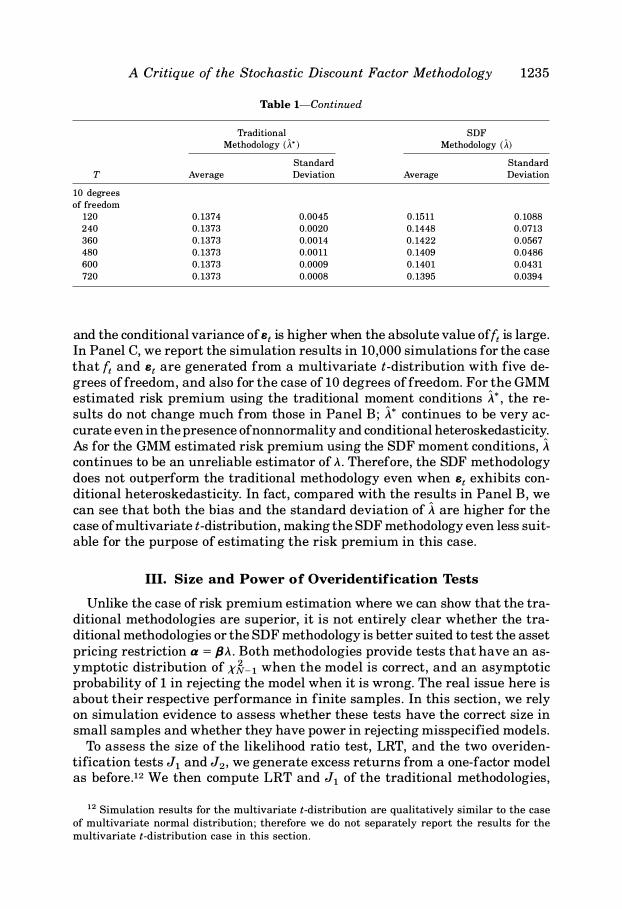
and the conditional variance of Bt is higher when the absolute value of ft is large. In Panel C, we report the simulation results in 10,000 simulations for the case that ft and et are generated from a multivariate t-distribution with five degrees of freedom, and also for the case of 10 degrees of freedom. For the GMM estimated risk premium using the traditional moment conditions A*, the results do not change much from those in Panel B; A* continues to be very accurate even in the presence ofnonnormality and conditional heteroskedasticity. As for the GMM estimated risk premium using the SDF moment conditions, A continues to be an unreliable estimator of..\. Therefore, the SDF methodology does not outperform the traditional methodology even when et exhibits conditional heteroskedasticity. In fact, compared with the results in Panel B, we can see that both the bias and the standard deviation of A are higher for the case of multivariate t-distribution, making the SDF methodology even less suitable for the purpose of estimating the risk premium in this case.
III. Size and Power of Overidentification Tests
Unlike the case of risk premium estimation where we can show that the traditional methodologies are superior, it is not entirely clear whether the traditional methodologies or the SDF methodology is better suited to test the asset pricing restriction a = fJ..\. Both methodologies provide tests that have an asymptotic distribution of x�-l when the model is correct, and an asymptotic probability of 1 in rejecting the model when it is wrong. The real issue here is about their respective performance in finite samples . In this section, we rely on simulation evidence to assess whether these tests have the correct size in small samples and whether they have power in rejecting misspecified models.
To assess the size of the likelihood ratio test, LRT, and the two overidentification tests J1 and J2, we generate excess returns from a one-factor model as before .12 We then compute LRT and J1 of the traditional methodologies,
12 Simulation results for the multivariate t-distribution are qualitatively similar to the case of multivariate normal distribution; therefore we do not separately report the results for the multivariate t-distribution case in this section.
1236 The Journal of Finance
and J2 of the SDF methodology for three different models. In the first model, we use the true factor ft to construct the sample moments and the test statistics . In the second model, we use a noisy factor gt = ( ft + nt )I .f5 instead of ft to compute the sample moment and the test statistics, where nt is a measurement error that is generated from a normal distribution with mean 0 and variance 4. In the final model, we specify the unsystematic factor ht = fJI-1etl� fJ'I-1fJ as the true factor to perform the test. Although economically these three factors are very different, statistically they are all considered to be correctly specified models.13 Therefore, asymptotically, all three tests should have an asymptotic distribution of x�-1 for the three correctly specified models .
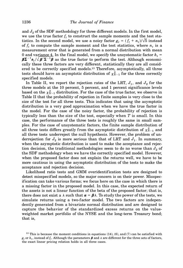
In Table II, we report the rejection rates of the LRT, J1, and J2 for the three models at the 10 percent, 5 percent, and 1 percent significance levels based on the x�-l distribution. For the case of the true factor, we observe in Table II that the probability of rejection in finite samples is very close to the size of the test for all three tests . This indicates that using the asymptotic distribution is a very good approximation when we have the true factor in the model. For the case of the noisy factor, the probability of rejection is typically less than the size of the test, especially when T is small. In this case, the performance of the three tests is roughly the same in small samples. For the case of unsystematic factors, the finite sample distribution of all three tests differs greatly from the asymptotic distribution of x�-1 and all three tests underreject the null hypothesis. However, the problem of underrejection for J2 is more serious than that of LRT and J1. In summary, when the asymptotic distribution is used to make the acceptance and rejection decision, the traditional methodologies seem to do no worse than J2 of the SDF methodology when we have the correctly specified model . However, when the proposed factor does not explain the returns well, we have to be more cautious in using the asymptotic distribution of the tests to make the acceptance and rejection decision.
Likelihood ratio tests and GMM overidentification tests are designed to detect misspecified models, so the major concern is on their power. Misspecification can take various forms; we focus here on the case in which there is a missing factor in the proposed model . In this case, the expected return of the assets is not a linear function of the beta of the proposed factor; that is, there does not exist a .A such that a = fl.-\. To study the power of the tests, we simulate returns using a two-factor model . The two factors are independently generated from a bivariate normal distribution and are designed to capture the behavior of the standardized excess returns on the valueweighted market portfolio of the NYSE and the long-term Treasury bond; that is,
13 This is because the moment conditions in equations (14), (6), and (7) can be satisfied with
g, or h,, instead of{,. Although the parameters fJ and A are different for the three sets of factors,
the exact linear pricing relation holds in all three cases.
A Critique of the Stochastic Discount Factor Methodology
Table II Size of the Likelihood Ratio Test and the GMM
Overidentification Tests of Traditional and Stochastic Discount Factor Methodologies
1237
The table presents the probability of rejecting three correctly specified models using the
likelihood ratio test (LRT) and the (second stage) GMM overidentification tests using the
traditional moment conditions and the SDF moment conditions. Excess returns on 10
assets are simulated using a one-factor model
r, = a + {Jf, + e,,
where the values of a = f3A (in percentage per month) and f3 are presented in Table I. The
factor and the model disturbance are generated as{,� N(0,1) and e, � N(ON,I), where I is set to equal the sample covariance matrix of the market model residuals of the 10
size-ranked portfolios of the NYSE, estimated using monthly returns over the period Jan
uary 1926 to December 1997. For each length of time-series observations, T, we present
the probability of rejecting three different models at various significance levels in 10,000 simulations. The three models differ in terms of the factor they use. The first model uses
the true factor {,. The second model uses a noisy factor g, = (f, + n ,)!J5, where n, is
measurement error, distributed as N(0,4). The third model uses an unsystematic factor
h, = f3'I,-le,!� {3'!.-l/3.
True Noisy Unsystematic
Significance Level Significance Level Significance Level
T 10% 5% 1% 10% 5% 1% 10% 5% 1%
Panel A: Maximum Likelihood Method (LRT)
120 0.099 0.048 0.010 0.082 0.037 0.007 0.013 0.003 0.001
240 0.098 0.047 0.008 0.090 0.042 0.007 0.026 0.008 0.001
360 0.098 0.048 0.010 0.093 0.043 0.008 0.035 0.012 0.001
480 0.098 0.048 0.009 0.090 0.046 0.007 0.040 0.015 0.002
600 0.099 0.049 0.011 0.092 0.047 0.009 0.052 0.022 0.002
720 0.101 0.050 0.012 0.098 0.048 0.011 0.059 0.024 0.004
Panel B: GMM Using Traditional Moment Conditions (J1)
120 0.093 0.043 0.007 0.076 0.032 0.006 0.017 0.004 0.000
240 0.097 0.046 0.009 0.088 0.042 0.008 0.025 0.007 0.000
360 0.099 0.049 0.010 0.095 0.045 0.008 0.031 0.010 0.000
480 0.099 0.049 0.010 0.095 0.048 0.009 0.041 0.016 0.001
600 0.097 0.046 0.010 0.096 0.046 0.008 0.048 0.017 0.002
720 0.102 0.048 0.010 0.098 0.047 0.009 0.053 0.020 0.002
Panel C: Stochastic Discount Factor Methodology (J2)
120 0.097 0.046 0.007 0.079 0.037 0.006 0.017 0.008 0.001
240 0.098 0.047 0.009 0.086 0.041 0.007 0.013 0.006 0.001
360 0.102 0.048 0.008 0.092 0.043 0.008 0.010 0.006 0.001
480 0.101 0.048 0.009 0.094 0.043 0.007 0.012 0.007 0.002
600 0.101 0.051 0.011 0.093 0.046 0.010 0.012 0.007 0.003
720 0.104 0.051 0.009 0.098 0.047 0.010 0.011 0.008 0.004
1238 The Journal of Finance
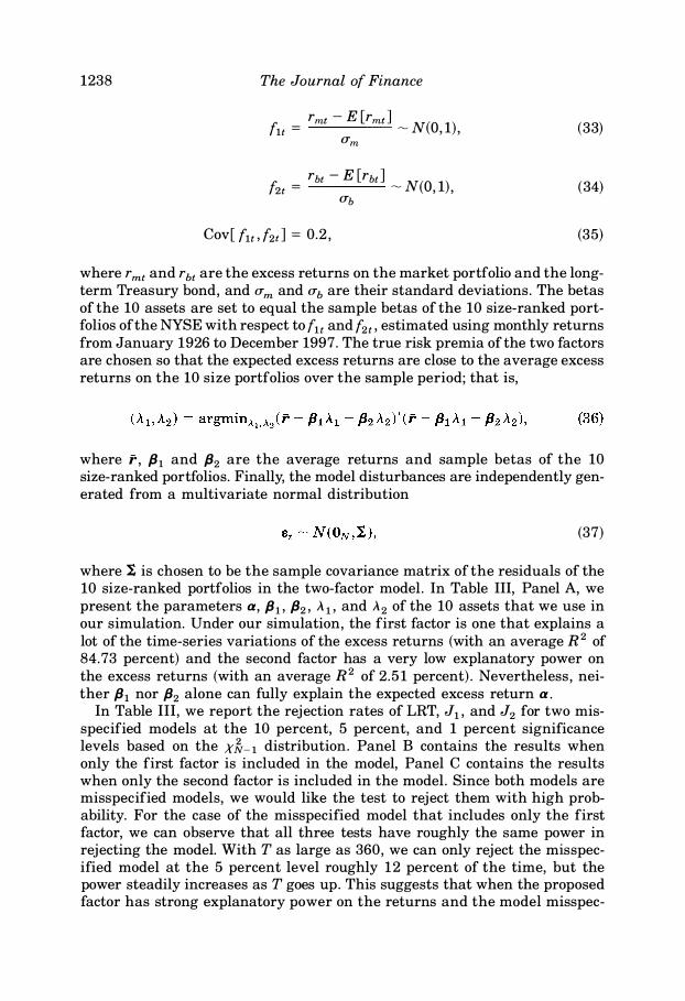
r - E[r ] f =
mt mt � N(O 1) 1 t ' '
Um
r - E[r ] f =
bt bt � N(O 1) 2t ' ' ub
Cov[ f1 tJ2t] = 0.2 ,
(33)
(34)
(35)
where r mt and rbt are the excess returns on the market portfolio and the longterm Treasury bond, and um and ub are their standard deviations . The betas of the 10 assets are set to equal the sample betas of the 10 size-ranked portfolios of the NYSE with respect to f1 t and f2t, estimated using monthly returns from January 1926 to December 1997. The true risk premia of the two factors are chosen so that the expected excess returns are close to the average excess returns on the 10 size portfolios over the sample period; that is,
where r, /31 and /32 are the average returns and sample betas of the 10 size-ranked portfolios. Finally, the model disturbances are independently generated from a multivariate normal distribution
(37)
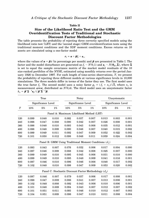
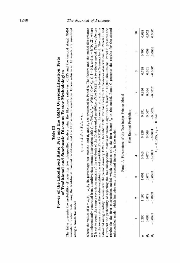
where I is chosen to be the sample covariance matrix of the residuals of the 10 size-ranked portfolios in the two-factor model . In Table III, Panel A, we present the parameters a, {31 , /32, A 1 , and A 2 of the 10 assets that we use in our simulation. Under our simulation, the first factor is one that explains a lot of the time-series variations of the excess returns (with an average R2 of 84.73 percent) and the second factor has a very low explanatory power on the excess returns (with an average R2 of 2 .51 percent) . Nevertheless , neither /31 nor /32 alone can fully explain the expected excess return a.
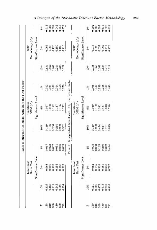
In Table III, we report the rejection rates of LRT, J1 , and J2 for two misspecified models at the 10 percent, 5 percent, and 1 percent significance levels based on the xlr- 1 distribution. Panel B contains the results when only the first factor is included in the model, Panel C contains the results when only the second factor is included in the model . Since both models are misspecified models, we would like the test to reject them with high probability. For the case of the misspecified model that includes only the first factor, we can observe that all three tests have roughly the same power in rejecting the model. With T as large as 360, we can only reject the misspecified model at the 5 percent level roughly 12 percent of the time, but the power steadily increases as T goes up. This suggests that when the proposed factor has strong explanatory power on the returns and the model misspec-
A Critique of the Stochastic Discount Factor Methodology 1239
ification is not serious, there is not much of a difference between the traditional methodologies and the SDF methodology.
Ironically, when the proposed factor in the model is a weak factor, the misspecified model becomes even more difficult to detect for the SDF methodology. This can be seen from our simulation results in Panel C of Table III. In this case, LRT and J1 have reasonably good power in rejecting this misspecified model. When T = 360, these two tests reject the misspecified model at the 5 percent level for approximately 34 percent of the time. However, J2 of the SDF methodology performs much worse than LRT and J1. Even for T = 360, we still find that J2 rejects the misspecified model less often than the size of the test, making it almost impossible to reject such a misspecified model . The poor performance of J2 in finite samples is due to the fact that 82 is unknown and has to be estimated. When the model is misspecified, the estimated 82 will tend to be large because of the pricing error, and hence its inverse will be small . Since the inverse of estimated 82 is used to compute J2, the test statistic can be very small for grossly misspecified models, especially when the factor does not explain much of the return. Asymptotically, this is not a concern because eventually the pricing errors will dominate as T increases, but in finite samples, using an estimated 82 makes the overidentification test J2 very unreliable. Although the same problem also plagues LRT and J1 of the traditional methodologies, we can see in Panel C that its impact on LRT and J1 is much less severe . Therefore, if one has to pick a specification test to use, it appears that the ones from the traditional methodologies are superior to the one from the SDF methodology.
We should also note that J2 of the SDF methodology seems to prefer models with a poor factor to the model with a good factor. This suggests, among other things, the danger of using the p-value of the likelihood ratio test or GMM overidentification test to choose models. In this regard, the traditional methodologies are superior because a poor factor is less likely to be proposed to be the only factor in the return-generating process. The SDF methodology does not specify a return-generating process and a poor factor could potentially be chosen as the only factor in the model . As our simulation experiment shows, such poor factors could make the model pass the GMM overidentification test of the SDF methodology easily, even though they do not explain much of the excess returns and their betas do not fully explain the expected excess returns.
As always, simulation evidence cannot be generalized to other scenarios, so our recommendation should be taken with caution. Nevertheless, from our simulation evidence, it does appear that there are compelling reasons to prefer the traditional methodologies to the SDF methodology. A more rigorous analysis of the size and power of these tests would go a long way in settling these issues.
Finally, we remark that even though nonstandard GMM overidentification tests, such as the one suggested by Jagannathan and Wang (1996), do not use the estimated covariance matrix of the sample moments to compute the test statistic, the estimated covariance matrix is still used in computing
Tabl
e II
I P
ow
er
of
the
Lik
eli
ho
od
Ra
tio
Te
st
an
d t
he
GM
M O
ve
rid
en
tifi
ca
tio
n T
es
ts
of
Tra
dit
ion
al
an
d S
toc
ha
sti
c D
isc
ou
nt
Fa
cto
r M
eth
od
olo
gie
s
Th
e t
ab
le
pre
sen
ts
the
pro
ba
bil
ity
o
f re
ject
ing
tw
o
mis
spe
cifi
ed
m
od
els
u
sin
g
the
li
ke
lih
oo
d r
ati
o
test
(L
RT
) a
nd
th
e
(se
con
d
sta
ge
) G
MM
ov
eri
de
nti
fica
tio
n t
est
s u
sin
g t
he
tra
dit
ion
al
mo
me
nt
con
dit
ion
s a
nd
th
e
SD
F m
om
en
t co
nd
itio
ns.
Ex
cess
re
turn
s o
n 1
0 a
sse
ts a
re s
imu
late
d
usi
ng
a t
wo
-fa
cto
r m
od
el
r, =
a+
fJ1f
11 +
fJ2f
2 t +
s,,
wh
ere
th
e v
alu
es
of
a =
A1
{J1 +
A2{J
2 (i
n p
erc
en
tag
e p
er
mo
nth
), a
nd
{J1
an
d {J
2 a
re p
rese
nte
d i
n P
an
el
A.
Th
e f
act
ors
an
d t
he
mo
de
l d
istu
rba
nce
are
in
de
pe
nd
en
tly
ge
ne
rate
d f
rom
a m
ult
iva
ria
te n
orm
al
dis
trib
uti
on
wit
h {1
, � N
(0,1
), { 2
, � N
(0,1
), C
ov
[ {1
1,{2,
] = 0
.2,
an
d s
, � N
(ON
,I),
wh
ere
I is
se
t to
eq
ua
l th
e s
am
ple
co
va
ria
nce
ma
trix
of
the
re
sid
ua
ls o
f th
e 1
0 s
ize
-ra
nk
ed
po
rtfo
lio
s o
f th
e NY
SE
in
a t
wo
-fa
cto
r m
od
el.
Th
e t
wo
fa
cto
rs
are
th
e e
xce
ss r
etu
rn o
n t
he
va
lue
-we
igh
ted
ma
rke
t p
ort
foli
o o
f th
e NY
SE
an
d t
he
ex
cess
re
turn
on
th
e l
on
g-t
erm
Tre
asu
ry b
on
d.
Th
e m
od
el
is
est
ima
ted
usi
ng
mo
nth
ly r
etu
rns
ov
er
the
pe
rio
d J
an
ua
ry 1
92
6 t
o D
ece
mb
er
19
97
. F
or
ea
ch l
en
gth
of
tim
e-s
eri
es
ob
serv
ati
on
s, T
, P
an
els
B a
nd
C p
rese
nt
the
pro
ba
bil
ity
of
reje
ctin
g t
he
tw
o m
issp
eci
fie
d m
od
els
at
va
rio
us
sig
nif
ica
nce
le
ve
ls i
n 1
0,0
00
sim
ula
tio
ns.
Pa
ne
l B
pre
sen
ts t
he
resu
lts
for
the
fi
rst
mis
spe
cifi
ed
m
od
el
wh
ich
in
clu
de
s o
nly
th
e
firs
t fa
cto
r {1
, in
th
e
mo
de
l.
Pa
ne
l C
p
rese
nts
th
e
resu
lts
for
the
se
con
d
mis
spe
cifi
ed
mo
de
l w
hic
h i
ncl
ud
es
on
ly t
he
se
con
d f
act
or
{ 21 i
n t
he
mo
de
l.
Pa
ne
l A
: P
ara
me
ters
of
the
Tw
o-f
act
or
Pri
cin
g M
od
el
Siz
e-R
an
ke
d P
ort
foli
os
1
2
3
4
5
6
7
8
9
10
a 1
.28
0
1.1
63
1
.00
1
0.9
40
0
.92
6
0.8
91
0
.83
6
0.7
48
0
.70
3
0.6
28
{J l
0.0
84
0
.07
9
0.0
73
0
.07
0
0.0
68
0
.06
7
0.0
64
0
.06
1
0.0
59
0
.05
2
fJ2
-0
.00
83
-
0.0
06
3
-0
.00
35
-
0.0
02
7
-0
.00
31
-
0.0
02
4
-0
.00
17
-
0.0
00
1
0.0
00
6
0.0
00
1
A1 =
0
.12
25
, A2
=
-0
.30
47
......
tv
>1>--
0 � (':)
�
;:: '1 � (:l .,_
�
'"lj
;:;·
(:l � �
(':)
Pa
ne
l B
: M
issp
eci
fie
d M
od
el
wit
h O
nly
th
e F
irst
Fa
cto
r
Lik
eli
ho
od
T
rad
itio
na
l S
DF
Ra
tio
Tes
t G
MM
(J1
) M
eth
od
olo
gy
(J2
) S
ign
ific
an
ce L
ev
el
Sig
nif
ica
nce
Le
ve
l S
ign
ific
an
ce L
ev
el
>
(")
T
10
%
5%
1
%
10
%
5%
1
%
10
%
5%
1
%
-; .....
.,.,.
12
0
0.1
29
0
.06
8
0.0
17
0
.11
9
0.0
57
0
.01
2
0.1
31
0
.06
6
0.0
12
.o
· !:: 2
40
0
.16
6
0.0
96
0
.02
3
0.1
66
0
.08
8
0.0
21
0
.16
2
0.0
88
0
.02
2
(I)
36
0
0.2
12
0
.12
3
0.0
37
0
.20
6
0.1
22
0
.03
2
0.2
07
0
.12
0
0.0
32
�
4
80
0
.24
5
0.1
53
0
.05
1
0.2
44
0
.14
7
0.0
44
0
.24
4
0.1
50
0
.04
2
.,.,.
�
60
0
0.2
90
0
.18
8
0.0
66
0
.28
9
0.1
85
0
.05
8
0.2
88
0
.18
0
0.0
57
(I)
72
0
0.3
34
0
.22
2
0.0
83
0
.33
2
0.2
22
0
.07
8
0.3
29
0
.21
3
0.0
78
\f.)
.,.,.
0
P
an
el
C:
Mis
spe
cifi
ed
Mo
de
l w
ith
On
ly t
he
Se
con
d F
act
or
("") �
Q L
ike
lih
oo
d
Tra
dit
ion
al
SD
F
"' .,.,.
Ra
tio
Tes
t G
MM
(J1
) M
eth
od
olo
gy
(J 2
) r;·
Sig
nif
ica
nce
Le
ve
l �
S
ign
ific
an
ce L
ev
el
Sig
nif
ica
nce
Le
ve
l c;;·
("")
T
10
%
5%
1
%
10
%
5%
1
%
10
%
5%
1
%
0 !:: ;:l
12
0
0.1
11
0
.05
2
0.0
08
0
.11
0
0.0
50
0
.00
6
0.0
38
0
.01
7
0.0
02
.,.,.
2
40
0
.29
5
0.1
85
0
.05
3
0.2
99
0
.18
2
0.0
47
0
.05
9
0.0
23
0
.00
3
� 3
60
0
.47
2
0.3
38
0
.13
5
0.4
74
0
.34
1
0.1
39
0
.08
1
0.0
37
0
.00
7
("") .,.,.
48
0
0.6
13
0
.48
1
0.2
46
0
.61
7
0.4
87
0
.24
8
0.1
34
0
.06
2
0.0
11
0
-; 6
00
0
.73
0
0.6
08
0
.36
2
0.7
31
0
.61
3
0.3
67
0
.21
9
0.1
10
0
.02
0
� 7
20
0
.81
6
0.7
17
0
.48
4
0.8
15
0
.71
0
0.4
80
0
.31
9
0.1
76
0
.03
9
.,.,.
�
0 Q...
0 ......
�
'<
f-'
l'V
....
f-'
1242 The Journal of Finance
the eigenvalues to construct the weights of the linear combination of x� distribution that the test statistic is compared with. Therefore, the nonstandard GMM overidentification test does not escape from the problem that plagues the standard GMM. Although not reported, simulation evidence suggests that the nonstandard GMM overidentification test that uses the identity matrix as the weighting matrix generally has lower power than that of the standard GMM overidentification test in detecting our misspecified models .
Iv. Conclusions
This paper exploits the fact that current empirical studies of asset pricing models using the SDF methodology typically ignore a fully specified model for asset returns . When asset returns are generated by a linear factor model, there are two potential problems associated with the use of the SDF methodology: (1) the accuracy of the estimated risk premium can be very poor and (2) its overidentification test has very little power in detecting misspecified models . These problems arise because the moment conditions the SDF methodology uses are very volatile, making accurate estimation and testing difficult under this methodology.
By specifying the return-generating process of the asset returns as in the traditional methodologies, these two potential problems can be mitigated. We demonstrate that, under the assumption that assets returns are generated by a linear factor model, the standard error of the risk premium under the traditional methodologies is much lower than that of the SDF methodology. The reason for such improvement is that the traditional methodologies use moment conditions that are much less volatile than that of the SDF methodology, and as a result they provide far more reliable inferences on the parameters . Moreover, the specification tests in the traditional methodologies generally have higher power in rejecting misspecified models than the SDF methodology. Our analysis focuses exclusively on linear factor models. This is not only due to their tractability, but also their premier importance in asset pricing. However, to the extent that any nonlinear model can be well approximated by a linear one, our results should also have implications on the use of the SDF methodology in nonlinear models where one must be cautious about the explanatory power of the factors, the parameter estimation error, the size, and the power of the tests .
Despite the fact that the SDF methodology has an interesting perspective to offer and a parsimonious model to estimate, there are costs associated with these benefits . In any event, it appears safe to say that the traditional methodologies are here to stay. In particular, traditional tests of asset pricing models will continue to play important roles in understanding the risks associated with investing, and perhaps even more so than the stochastic discount factor methodology for portfolio choice and performance evaluation problems .
A Critique of the Stochastic Discount Factor Methodolog y 1243
Appendix
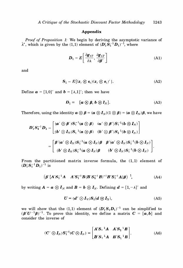
Proof of Proposition 1: We begin by deriving the asymptotic variance of A*, which is given by the (1,1) element of (Di S1 1 D1 )-\ where
and
D = E [ i)g1T i)g1T ] 1 i)A. ' iJfJ '
Define a = [1,0] ' and b = [A.,1] ' ; then we have
(A1)
(A2)
(A3)
Therefore, using the identity a ® fJ = (a ® IN) (1 ® fJ) = (a ® IN)fJ, we have
= [fJ ' (a ' @ IN)S11 (a @ IN)fJ fJ ' (a ' @ IN)S11 (b @ IN) ]
. (b ' @ IN)S1 1 (a @ IN)fJ (b ' @ IN)S1 1 (b @ IN)
From the partitioned matrix inverse formula, the (1, 1) element of (D)_ 81 1 D1 )-1 is
(A4)
by writing A = a ® IN and B = b ® IN . Defining d = [1, - A.] ' and
(A5)
we will show that the (1,1) element of (Dl_ S1D1 )- 1 can be simplified to ( fJ ' U- 1/J )-1 . To prove this identity, we define a matrix C = [a, b] and consider the inverse of
(A6)
1244 The Journal of Finance
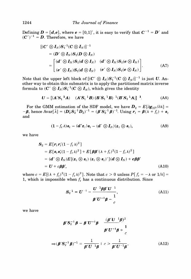
Defining D = [d, e] , where e = [0, 1] ' , it is easy to verify that c - 1 = D ' and (C ' )- 1 = D. Therefore, we have
[(C ' (8)1N)S1 1 (C (8)/N)] - 1
= (D ' @ IN)S1 (D @ IN)
= [ (d ' @ IN)S1 (d @ IN) (d ' ® IN)S1 (e ® IN) ]
. (A7) (e ' @ IN)S1(d @ IN) (e ' @ IN)S1(e @ IN)
Note that the upper left block of [(C ' ® IN)S11 (C ® IN)r 1 i s just U. Another way to obtain this submatrix is to apply the partitioned matrix inverse formula to (C ' ® IN)S1 1 (C ® IN) , which gives the identity
For the GMM estimation of the SDF model, we have D2 = E [dg2r/dA.] = -fJ, hence Avar[A] = (D2 Si. 1 D2 )-1 = (fJ 'Si. 1 fJ )- 1. Using r1 = fJ (.A + ft ) + 81 and
we have
82 = E [r1 r; ( 1 - {1 .A) 2 ]
= E [e1 e; ( l - ft .A) 2 ] + E [fJfJ ' (A. + ft ) 2 ( 1 - ft .A) 2 ]
= (d ' ® IN)E [(z1 ® 81 ) (z 1 ® B1 ) ' ] (d ® IN) + cfJfJ '
= U + cfJfJ ',
(A9)
(A10)
where c = E [(.A + ft ) 2 ( 1 - {1 .A) 2 ] . Note that c > 0 unless P [ {1 = - A. or 1/.A] = 1 , which is impossible when ft has a continuous distribution. Since
(All)
we have
(A12)
A Critique of the Stochastic Discount Factor Methodolog y 1245
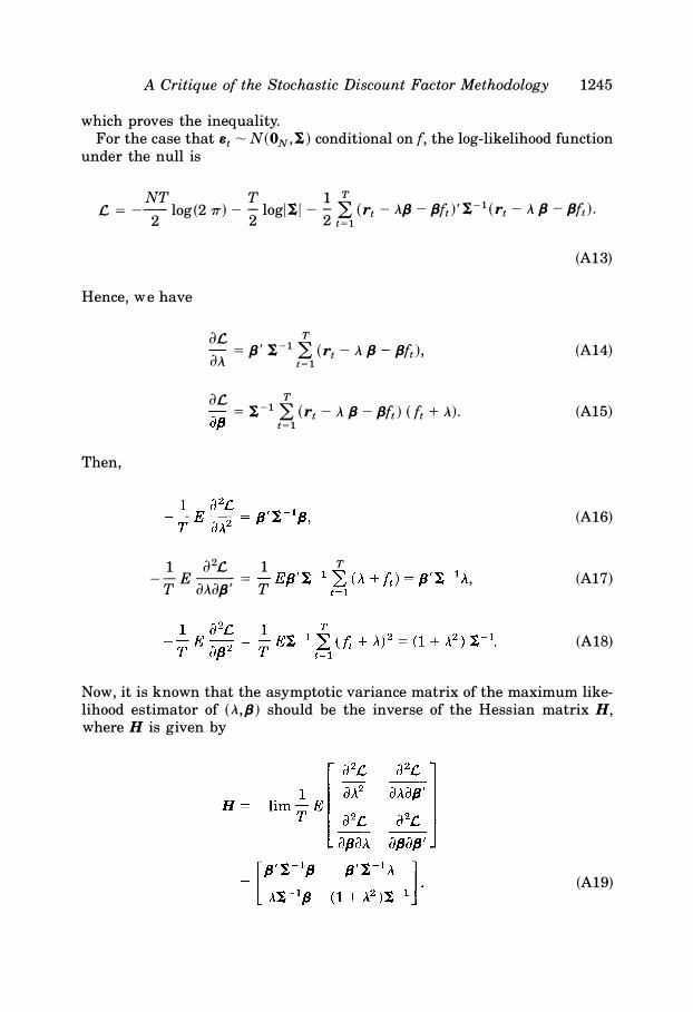
which proves the inequality. For the case that e1 � N(ON, I) conditional on {, the log-likelihood function
under the null is
NT T 1 T ' -1 £ = -2 log (2 1r ) - 2 log i i i - 2 �� (r1 - A{J - fJ{1 ) I ( r1 - A fJ - fJ{1 ) .
Hence, w e have
Then,
(JC T
dA = fJ ' I-1 � ( rt - A fJ - fJft ) ,
()£ T -;-- = I-1 2: (rt - A fJ - fJft ) ( ft + A) . ufJ t� 1
1 () 2£ 1 T - - E -- = - EfJ' I - 1 " ( A + -�" ) = fJ ' I- 1A
T dAdfJ ' T � I t '
(A13)
(A14)
(A15)
(A16)
(A17)
(A18)
Now, it is known that the asymptotic variance matrix of the maximum likelihood estimator of (A , fJ ) should be the inverse of the Hessian matrix H, where H is given by
(A19)
1246 The Journal of Finance
When Bt - N(ON , I ) conditional on f, we have 81 = 12 ® I and H has the same expression as D)_ 811 D1 . This completes the proof. Note that our proof only depends on rt having a factor structure and the beta pricing model holding; it does not require the true factor ft . Therefore, Proposition 1 continues to hold when gt or ht is used as the factor. •
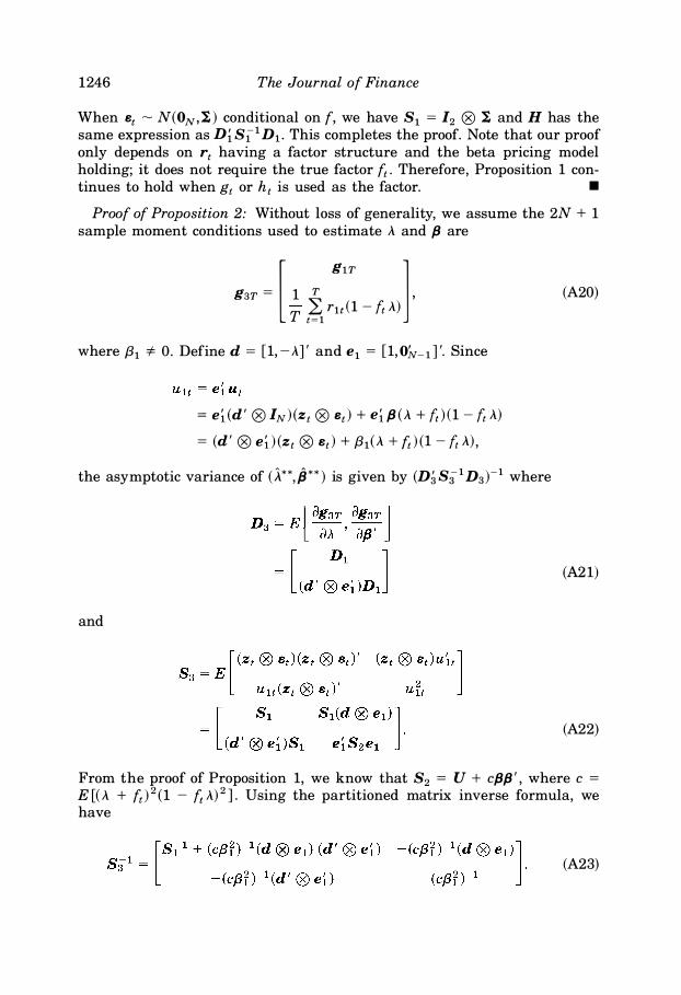
Proof of Proposition 2: Without loss of generality, we assume the 2N + 1 sample moment conditions used to estimate .A and fJ are
r glT
1 g3T = 1 T ,
T t� r lt(1 - ft .A)
where {31 * 0. Define d = [ 1, - .A] ' and e1 = [ 1, 01v- d '. Since
= ei_ (d ' <8) /N ) (Z t <8) Bt ) + ei_ fJ (.A + ft)(1 - ft .A)
= (d ' ® ei_ ) (zt ® Bt ) + {31 (.A + ft ) (1 - ft .A) ,
the asymptotic variance of (A**, fj**) is given by (D3 S3 1 D3 )- 1 where
and
(A20)
(A2 1)
(A22)
From the proof of Proposition 1, we know that 82 = U + cfJfJ ' , where c = E [( .A + ft ) 2 ( 1 - ft .A) 2 ] . Using the partitioned matrix inverse formula, we have
(A23)
A Critique of the Stochastic Discount Factor Methodology
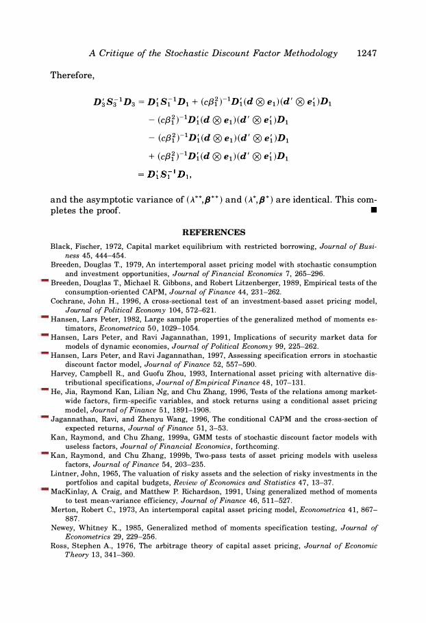
Therefore,
D3 S3 1 D3 = Di S! 1 D1 + (c{3[ )-1Di (d ® e1 ) (d ' ® ei )D1
- (cf3f )-1Dl_ (d ® e1 ) (d ' ® ei )D1
- (cf3f )-1Dl_ (d ® e1 ) (d ' ® ei )D1
+ (c{3f )-1Di (d ® e1 ) (d ' ® ei )D1
1247
and the asymptotic variance of (Jt.**, /J * * ) and (Jt.*, /J * ) are identical . This completes the proof. •
REFERENCES
Black, Fischer, 1972, Capital market equilibrium with restricted borrowing, Journal of Busi
ness 45, 444--454.
Breeden, Douglas T., 1979, An intertemporal asset pricing model with stochastic consumption
and investment opportunities, Journal of Financial Economics 7, 265-296.
Breeden, Douglas T., Michael R. Gibbons, and Robert Litzenberger, 1989, Empirical tests of the
consumption-oriented CAPM, Journal of Finance 44, 231-262.
Cochrane, John H., 1996, A cross-sectional test of an investment-based asset pricing model,
Journal of Political Economy 104, 572--621.
Hansen, Lars Peter, 1982, Large sample properties of the generalized method of moments es
timators, Econometrica 50, 1029-1054.
Hansen, Lars Peter, and Ravi Jagannathan, 1991, Implications of security market data for
models of dynamic economies, Journal of Political Economy 99, 225-262.
Hansen, Lars Peter, and Ravi Jagannathan, 1997, Assessing specification errors in stochastic
discount factor model, Journal of Finance 52, 557-590.
Harvey, Campbell R., and Guofu Zhou, 1993, International asset pricing with alternative dis
tributional specifications, Journal of Empirical Finance 48, 107-131.
He, Jia, Raymond Kan, Lilian Ng, and Chu Zhang, 1996, Tests of the relations among market
wide factors, firm-specific variables, and stock returns using a conditional asset pricing
model, Journal of Finance 51, 1891-1908.
Jagannathan, Ravi, and Zhenyu Wang, 1996, The conditional CAPM and the cross-section of
expected returns, Journal of Finance 51, 3-53.
Kan, Raymond, and Chu Zhang, 1999a, GMM tests of stochastic discount factor models with
useless factors, Journal of Financial Economics, forthcoming.
Kan, Raymond, and Chu Zhang, 1999b, Two-pass tests of asset pricing models with useless
factors, Journal of Finance 54, 203-235.
Lintner, John, 1965, The valuation of risky assets and the selection of risky investments in the
portfolios and capital budgets, Review of Economics and Statistics 47, 13-37.
MacKinlay, A. Craig, and Matthew P. Richardson, 1991, Using generalized method of moments
to test mean-variance efficiency, Journal of Finance 46, 511-527.
Merton, Robert C., 1973, An intertemporal capital asset pricing model, Econometrica 41, 867-
887.
Newey, Whitney K., 1985, Generalized method of moments specification testing, Journal of
Econometrics 29, 229-256.
Ross, Stephen A., 1976, The arbitrage theory of capital asset pricing, Journal of Economic Theory 13, 341-360.

1248 The Journal of Finance
Sharpe, William F., 1964, Capital asset prices: A theory of market equilibrium under conditions
of risk, Journal of Finance 19, 425-442.
Zhou, Guofu, 1991, Small sample tests of portfolio efficiency, Journal of Financial Economics
30, 165-191.
Zhou, Guofu, 1994, Analytical GMM tests: Asset pricing with time-varying risk premiums, Re
view of Financial Studies 7, 687-709.
Zhou, Guofu, 1995, Small sample rank tests with applications to asset pricing, Journal of Em
pirical Finance 2, 71-93.
Recommended