Embed Size (px)
Citation preview

A Stochastic Discount Factor Approach to Asset
Pricing using Panel Data Asymptotics∗
Fabio Araujo
Department of Economics
Princeton University
email: [email protected]
João Victor Issler
Graduate School of Economics —EPGE
Getulio Vargas Foundation
email: [email protected]†
This Draft: August, 2012.
Keywords: Stochastic Discount Factor, No-Arbitrage, Common
Features, Panel-Data Econometrics.
J.E.L. Codes: C32, C33, E21, E44, G12.
Abstract∗This paper circulated in 2005-6 as “A Stochastic Discount Factor Approach without a Utility Func-
tion.”Marcelo Fernandes was also a co-author in it. Since then, Fernandes has withdrawn from the paperand this draft includes solely the contributions of Araujo and Issler to that previous effort. We thank thecomments given by Jushan Bai, Marco Bonomo, Luis Braido, Xiaohong Chen, Valentina Corradi, CarlosE. Costa, Daniel Ferreira, Luiz Renato Lima, Oliver Linton, Humberto Moreira, Walter Novaes, andFarshid Vahid. We also thank José Gil Ferreira Vieira Filho and Rafael Burjack for excellent researchassistance. The usual disclaimer applies. Fabio Araujo and João Victor Issler gratefully acknowledgesupport given by CNPq-Brazil and Pronex. Issler also thanks INCT and FAPERJ for financial support.†Corresponding author: Graduate School of Economics, Getulio Vargas Foundation, Praia de Botafogo
190 s. 1100, Rio de Janeiro, RJ 22253-900, Brazil.
1

Using the Pricing Equation in a panel-data framework, we construct a novel
consistent estimator of the stochastic discount factor (SDF) which relies on the fact
that its logarithm is the “common feature” in every asset return of the economy.
Our estimator is a simple function of asset returns and does not depend on any
parametric function representing preferences.
The techniques discussed in this paper were applied to two relevant issues in
macroeconomics and finance: the first asks what type of parametric preference-
representation could be validated by asset-return data, and the second asks whether
or not our SDF estimator can price returns in an out-of-sample forecasting exercise.
In formal testing, we cannot reject standard preference specifications used in
the macro/finance literature. Estimates of the relative risk-aversion coeffi cient are
between 1 and 2, and statistically equal to unity.
We also show that our SDF proxy can price reasonably well the returns of stocks
with a higher capitalization level, whereas it shows some diffi culty in pricing stocks
with a lower level of capitalization.
2

1 Introduction
In this paper, we derive a novel consistent estimator of the stochastic discount factor (or
pricing kernel) that takes seriously the consequences of the Pricing Equation established
by Harrison and Kreps (1979), Hansen and Richard (1987), and Hansen and Jagannathan
(1991), where asset prices today are a function of their expected future payoffs discounted
by the stochastic discount factor (SDF). If the Pricing Equation is valid for all assets at
all times, it can serve as a basis to construct an estimator of the SDF in a panel-data
framework when the number of assets and time periods is suffi ciently large. This is exactly
the approach taken here.
We start with a general Taylor Expansion of the Pricing Equation to derive the de-
terminants of the logarithm of returns once we impose the moment restriction implied by
the Pricing Equation. The identification strategy employed to recover the logarithm of
the SDF relies on one of its basic properties —it is a “common feature,” in the sense of
Engle and Kozicki (1993), of every asset return of the economy. Under mild restrictions
on the behavior of asset returns, used frequently elsewhere, we show how to construct a
consistent estimator for the SDF which is a simple function of the arithmetic and geo-
metric averages of asset returns alone, and does not depend on any parametric function
used to characterize preferences.
A major benefit of our approach is that we are able to study intertemporal asset pricing
without the need to characterize preferences or to use of consumption data; see a similar
approach by Hansen and Jagannathan (1991, 1997). This yields several advantages of
our SDF estimator over possible alternatives. First, since it does not depend on any
parametric assumptions about preferences, there is no risk of misspecification in choosing
an inappropriate functional form for the estimation of the SDF. Moreover, our estimator
can be used to test directly different parametric-preference specifications commonly used
in finance and macroeconomics. Second, since it does not depend on consumption data,
our estimator does not inherit the smoothness observed in previous consumption-based
estimates which generated important puzzles in finance and in macroeconomics, such
as excess smoothness (excess sensitivity) in consumption, the equity-premium puzzle,
3

etc.; see Hansen and Singleton (1982, 1983, 1984), Mehra and Prescott (1985), Campbell
(1987), Campbell and Deaton (1989), and Epstein and Zin (1991).
Our approach is related to research done in three different fields. From econometrics,
it is related to the common-features literature after Engle and Kozicki (1993). Indeed,
we attempt to bridge the gap between a large literature on serial-correlation common
features applied to macroeconomics, e.g., Vahid and Engle (1993, 1997), Engle and Issler
(1995), Issler and Vahid (2001, 2006), Vahid and Issler (2002), Hecq, Palm and Urbain
(2005), Issler and Lima (2009), Athanasopoulos et al. (2011), and the financial econo-
metrics literature related to the SDF approach, perhaps best represented by Chapman
(1998), Aït-Sahalia and Lo (1998, 2000), Rosenberg and Engle (2002), Garcia, Luger, and
Renault (2003), Garcia, Renault, and Semenov (2006), Hansen and Scheinkman (2009),
and Hansen and Renault (2009). It is also related respectively to work on common fac-
tors in macroeconomics and in finance; see Geweke (1977), Stock and Watson (1989,
1993, 2002) Forni et al. (2000), and Bai and Ng (2004) as examples of the former, and
a large literature in finance perhaps best exemplified by Fama and French (1992, 1993),
Lettau and Ludvigson (2001), Sentana (2004), and Sentana, Calzolari, and Fiorentini
(2008) as examples of the latter. In financial econometrics, we propose an alternative way
of imposing no-arbitrage in constructing important estimators, which became popular in
through the work of Diebold and Li (2006), Christensen, Diebold, and Rudebusch (2009,
2011), and Diebold and Rudebusch (2013). From macroeconomics, it is related to the
work using panel data for testing optimal behavior in consumption, e.g., Runkle (1991),
Blundell, Browning, and Meghir (1994), Attanasio and Browning (1995), Attanasio and
Weber (1995), and to the work of Mulligan (2002) on cross-sectional aggregation and
intertemporal substitution.
The set of assumptions needed to derive our results are common to many papers in
financial econometrics: the lack of arbitrage opportunities in pricing securities is assumed
in virtually all studies estimating the SDF, and the restrictions (discipline) we impose on
the stochastic behavior of asset returns are fairly standard. What we see as non-standard
in our approach is an attempt to bridge the gap between economic and econometric theory
4

in devising an econometric estimator of a random process which has a straightforward
economic interpretation: it is the common feature of asset returns. Once the estimation
problem is put in these terms, it is straightforward to apply panel-data techniques to
construct a consistent estimator for the SDF. By construction, it will not depend on any
parametric function used to characterize preferences, which we see as a major benefit
following the arguments in the seminal work of Hansen and Jagannathan (1991, 1997).
In a first application, with quarterly data on U.S.$ real returns, ultimately using thou-
sands of assets available to the average U.S. investor, our estimator of the SDF is close
to unity most of the time and bound by the interval [0.85, 1.15], with an equivalent av-
erage annual discount factor of 0.9711, or an average annual real discount rate of 2.97%.
When we examined the appropriateness of different functional forms to represent prefer-
ences, we concluded that standard preference representations cannot be rejected by the
data. Moreover, estimates of the relative risk-aversion coeffi cient are close to what can
be expected a priori —between 1 and 2, statistically significant, and not different from
unity in statistical tests. In a second application, we tried to approximate the asymptotic
environment directly, working with monthly U.S. time-series return data with T = 336
observations, collected for a total of N = 16, 193 assets. Using the δ distance measure of
Hansen and Jagannathan (1997), we show that our SDF proxy can price reasonably well
the returns of stocks with a high capitalization value, although it shows some diffi culty in
pricing stocks of firms with a low level of capitalization.
The next Section presents basic theoretical results, our estimation techniques, and a
discussion of our main result. Section 3 shows the results of empirical tests in macro-
economics and finance using our estimator: estimating preference parameters using the
Consumption-based Capital Asset-Pricing Model (CCAPM) and out-of-sample evaluation
of the Asset-Pricing Equation. Section 4 concludes.
5

2 Economic Theory and SDF Estimator
2.1 A Simple Consistent Estimator
Harrison and Kreps (1979), Hansen and Richard (1987), and Hansen and Jagannathan
(1991) describe a general framework to asset pricing, associated to the stochastic discount
factor (SDF), which relies on the Pricing Equation1:
Et {Mt+1xi,t+1} = pi,t, i = 1, 2, . . . , N, or (1)
Et {Mt+1Ri,t+1} = 1, i = 1, 2, . . . , N, (2)
where Et(·) denotes the conditional expectation given the information available at time
t, Mt is the stochastic discount factor, pi,t denotes the price of the i-th asset at time t,
xi,t+1 denotes the payoff of the i-th asset in t+ 1, Ri,t+1 =xi,t+1pi,t
denotes the gross return
of the i-th asset in t+ 1, and N is the number of assets in the economy.
The existence of a SDF Mt+1 that prices assets in (1) is obtained under very mild
conditions. In particular, there is no need to assume a complete set of security markets.
Uniqueness of Mt+1, however, requires the existence of complete markets. If markets
are incomplete, i.e., if they do not span the entire set of contingencies, there will be an
infinite number of stochastic discount factors Mt+1 pricing all traded securities. Despite
that, there will still exist a unique discount factorM∗t+1, which is an element of the payoff
space, pricing all traded securities. Moreover, any discount factorMt+1 can be decomposed
as the sum of M∗t+1 and an error term orthogonal to payoffs, i.e., Mt+1 = M∗
t+1 + νt+1,
where Et (νt+1xi,t+1) = 0. The important fact here is that the pricing implications of any
Mt+1 are the same as those of M∗t+1, also known as the mimicking portfolio.
We now state the four basic assumptions needed to construct our estimator:
Assumption 1: We assume the absence of arbitrage opportunities in asset pricing, c.f.,
Ross (1976). This must hold instantaneously for all t = 1, 2, ..., T , i.e., it must hold
at all times and for all lapses of time, however small.
1See also Rubinstein(1976) and Ross(1978).
6

Assumption 2: Let Rt = (R1,t, R2,t, ... RN,t)′ be an N × 1 vector stacking all asset
returns in the economy and consider the vector process {ln (MtRt)}. In the time
(t) dimension, we assume that {ln (MtRt)}∞t=1 is covariance-stationary and ergodic
with finite first and second moments uniformly across i.
At a basic level, Assumption 1 is a necessary and suffi cient condition for the Pric-
ing Equation (2) to hold; see Cochrane (2002). Under the assumptions in Hansen and
Renault (2009), Assumption 1 implies (2). In any case, (2) is present, either implicitly
or explicitly, in virtually all studies in finance and macroeconomics dealing with asset
pricing and/or with intertemporal substitution; see, e.g., Hansen and Singleton (1982,
1983, 1984), Mehra and Prescott (1985), Epstein and Zin (1991), Fama and French (1992,
1993), Attanasio and Browning (1995), Lettau and Ludvigson (2001), Garcia, Renault,
and Semenov (2006), Hansen and Scheinkman (2009) and Hansen and Renault (2009). It
is essentially equivalent to the “law of one price”—where securities with identical payoffs
in all states of the world must have the same price. We impose its validity instantaneously
since we will derive a logarithmic representation for (2), which allows exact measure of
instantaneous returns for all assets.
The absence of arbitrage opportunities has also two other important implications. The
first is there exists at least one stochastic discount factorMt, for whichMt > 0; see Hansen
and Jagannathan (1997). This is due to the fact that, when we consider the existence
derivatives on traded assets, arbitrage opportunities will arise if Mt ≤ 0. Positivity of
some Mt is required here because we will take logs of Mt in proving our asymptotic
results2. The second is that the absence of arbitrage requires that a weak law-of-large
numbers (WLLN) holds in the cross-sectional dimension for the level of gross returns Ri,t
(Ross (1976, p. 342)). This controls the degree of cross-sectional dependence in the data
and constitutes the basis of the arbitrage pricing theory (APT). Applying the Ergodic
Theorem in the cross-sectional dimension, implies that we should also expect a WLLN to
hold for its logarithmic counterpart (lnRi,t), forming the basis of our asymptotic results.
2Recall that all CCAPM studies implicitly assume Mt > 0, since Mt = β u′(ct)u′(ct−1)
> 0, where ct isconsumption, β ∈ (0, 1) and u′ (·) > 0.
7

Assumption 2 controls the degree of time-series dependence in the data. Across time
(t), asset returns have clear signs of heterogeneity: different means and variances, and con-
ditional heteroskedasticity; as examples of the latter see Bollerslev, Engle and Wooldridge
(1988) and Engle and Marcucci (2006). Of course, weak-stationary processes can display
conditional heteroskedasticity as long as second moments are finite; see Engle (1982).
Therefore, Assumption 2 allows for heterogeneity in mean returns and conditional het-
eroskedasticity in returns used in computing our estimator. Uniformity across (i) is re-
quired for technical reasons, since we want the mean across first and second moments of
returns to be defined.
To construct a consistent estimator for {Mt} we consider a second-order Taylor Ex-
pansion of the exponential function around x, with increment h, as follows:
ex+h = ex + hex +h2ex+λ(h)·h
2, (3)
with λ(h) : R→ (0, 1) . (4)
It is important to stress that (3) is an exact relationship and not an approximation. This
is due to the nature of the function λ(h) : R → (0, 1), which maps into the open unit
interval. Thus, the last term is evaluated between x and x+h, making (3) to hold exactly.
For the expansion of a generic function, λ(·) would depend on x and h. However,
dividing (3) by ex:
eh = 1 + h+h2eλ(h)·h
2, (5)
shows that (5) does not depend on x. Therefore, we get a closed-form solution for λ(·) as
function of h alone:
λ(h) =
1h× ln
[2×(eh−1−h)
h2
], h 6= 0
1/3, h = 0,
where λ(·) maps from the real line into (0, 1). To connect (5) with the Pricing Equation
(2), we impose h = ln(MtRi,t) in (5) to obtain:
MtRi,t = 1 + ln(MtRi,t) +[ln(MtRi,t)]
2 eλ(ln(MtRi,t))·ln(MtRi,t)
2, (6)
8

which shows that the behavior of MtRi,t will be governed solely by that of ln(MtRi,t).
It is useful to define the random variable collecting the higher order term of (6):
zi,t ≡1
2× [ln(MtRi,t)]
2 eλ(ln(MtRi,t))·ln(MtRi,t).
Taking the conditional expectation of both sides of (6) gives:
Et−1 (MtRi,t) = 1 + Et−1 (ln(MtRi,t)) + Et−1 (zi,t) . (7)
As a direct consequence of the Pricing Equation, the left-hand side cancels with the first
term of the right-hand side of (7), yielding:
Et−1 (zi,t) = −Et−1 {ln(MtRi,t)} . (8)
This first shows that Et−1 (zi,t) will be solely a function of Et−1 {ln(MtRi,t)} if the
Pricing Equation holds, otherwise it will also be a function of Et−1(MtRi,t). Second,
zi,t ≥ 0 for all (i, t). Therefore, Et−1 (zi,t) ≡ γ2i,t ≥ 0, and we denote it as γ2i,t to stress the
fact that it is non-negative.
Let γ2t ≡(γ21,t, γ
22,t , ..., γ
2N,t
)′and εt ≡ (ε1,t, ε2,t, ..., εN,t)
′ stack respectively the condi-
tional means γ2i,t and the forecast errors εi,t. Then, from the definition of εt we have:
ln(MtRt) = Et−1{ln(MtRt)}+ εt
= −γ2t + εt. (9)
Denoting by rt = ln (Rt), which elements are denoted by ri,t = ln (Ri,t), and by mt =
ln (Mt), (9) yields the following system of equations:
ri,t = −mt − γ2i,t + εi,t, i = 1, 2, . . . , N. (10)
The system (10) shows that the (log of the) SDF is a common feature, in the sense
of Engle and Kozicki (1993), of all (logged) asset returns. For any two economic series,
9

a common feature exists if it is present in both of them and can be removed by linear
combination. Hansen and Singleton (1983) were the first authors to exploit this property
of (logged) asset returns, although the concept was only proposed 10 years later by Engle
and Kozicki.
Looking at (10), asset returns are decomposed into three terms, but we focus on the
first — the logarithm of the SDF, mt, which is common to all returns and has random
variation only across time. Notice that mt can be removed by linearly combining returns:
for any two assets i and j, ri,t − rj,t will not contain the feature mt, which makes (1,−1)
a “cofeature vector”for all asset pairs.
We label (10) as a quasi-structural system for logged returns, since its foundation is
the Asset-Pricing Equation (1). Equation (10) can be thought as a factor model for ri,t,
where the common factormt has only time-series variation. Indeed, this is the logarithmic
counterpart of the common-factor model assumed by Ross (1976) for the level of returns
Ri,t, where here the Pricing Equation (1) provides a solid structural foundation to it.
The sources of cross-sectional variation in every equation of the system (10) are εi,t
and γ2i,t. However, as we show next, the terms γ2i,t are a linear function of lagged εi,t, tying
the cross-sectional variation in (10) ultimately to εi,t.
Start with Assumption 2. Because ln(MtRt) is weakly stationary, for every one of its
elements ln(MtRi,t), there exists a Wold representation, which is a linear function of the
innovation in ln(MtRi,t), defined as εi,t = ln(MtRi,t) − Et−1{ln(MtRi,t)} and stacked in
εt ≡ (ε1,t, ε2,t, ..., εN,t)′. Therefore, the individual Wold representations can be written
as:
ln(MtRi,t) = µi +∞∑j=0
bi,jεi,t−j, i = 1, 2, . . . , N, (11)
where, for all i, bi,0 = 1, |µi| < ∞,∑∞
j=0 b2i,j < ∞, and εi,t is a multivariate white noise.
Using (8), in light of (11), leads to:
γ2i ≡ E(zi,t) = −E {ln(MtRi,t)} = −µi, (12)
which is well defined and time-invariant under Assumption 2. Taking conditional expec-
10

tations Et−1 (·) of (11), allows computing γ2i,t = Et−1 (zi,t) = −E {ln(MtRi,t)}, leading to
the following system, once we consider (10):
ri,t = −mt − γ2i + εi,t −∞∑j=1
bi,jεi,t−j, i = 1, 2, . . . , N. (13)
This is just a different way of writing (10)3. Because mt is devoid of cross-sectional
variation, (13) shows that the ultimate source of cross-sectional variation for ri,t is εi,t
(and its lags). This paves the way to derive a consistent estimator for Mt based on the
existence of a WLLN for {εi,t}Ni=1. This is consistent with limN→∞
V AR(1N
∑Ni=1 εi,t
)= 0,
but the critical issue is whether or not 1N
∑Ni=1 εi,t
p−→ 0. If that were the case, it would
be straightforward to compute plimN→∞
1N
∑Ni=1 ri,t + mt and then construct a a consistent
estimator for Mt.
Convergence in probability for logged returns ri,t is not surprising, given the assump-
tion of convergence in probability for the levels of returns Ri,t behind the APT. After all,
ri,t = ln (Ri,t) is a measurable transformation of Ri,t. By applying the Ergodic Theorem
in the cross-sectional dimension, we should also expect that a WLLN holds for {ri,t}Ni=1as well. Despite that, one may be skeptical of:
1
N
N∑i=1
εi,tp−→ 0. (14)
Equation (14) may seem restrictive because we can always decompose εi,t as:
εi,t = ln(MtRi,t)− Et−1{ln(MtRi,t)} (15)
= [mt − Et−1 (mt)] + [ri,t − Et−1 (ri,t)] = qt + vi,t, (16)
3Here it becomes obvious that:
γ2i,t = γ2i +
∞∑j=1
bi,jεi,t−j
= −µi +∞∑j=1
bi,jεi,t−j .
11

where qt = [mt − Et−1 (mt)] is the innovation in mt and vi,t = [ri,t − Et−1 (ri,t)] is the
innovation in ri,t. Therefore, to get plimN→∞
1N
∑Ni=1 εi,t = 0, we need,
plimN→∞
1
N
N∑i=1
vi,t = −qt, (17)
which may seem like a knife-edge restriction on the cross-sectional distribution of vi,t.
Indeed, it is not. To show it, consider the argument of projecting vi,t into qt, collecting
terms, and decomposing εi,t as follows:
εi,t = δiqt + ξi,t, where δi ≡COV (εi,t, qt)
VAR (qt)= 1 +
COV (vi,t, qt)
VAR (qt). (18)
Here, we collect all that is pervasive in qt and thus it is reasonable to assume that
plimN→∞
1N
∑Ni=1 ξi,t = 0. In this context of the factor model (18), in order to get plim
N→∞
1N
∑Ni=1 εi,t =
0, we must have:
plimN→∞
1
N
N∑i=1
ξi,t = −δqt, where limN→∞
1
N
N∑i=1
δi = δ. Thus, (19)
limN→∞
1
N
N∑i=1
δi = δ = 0, or limN→∞
1
N
N∑i=1
COV (vi,t, qt)
VAR (qt)= −1. (20)
Equation (20) highlights that the issue is not one of a knife-edge restriction. In order
to obtain plimN→∞
1N
∑Ni=1 εi,t = 0, and use plim
N→∞
1N
∑Ni=1 ri,t + mt to construct a consistent
estimator for Mt, the average factor loading must obey limN→∞
1N
∑Ni=1 δi = 0. Notice that
vi,t is an innovation coming from data (ri,t), but qt is an innovation coming from the latent
variable mt, which makes this an issue of separate identification of the factor (qt) and of
its respective factor loadings (δi).
Next, we state our most important result: a novel consistent estimator of the sto-
chastic process {Mt}∞t=1. Instead of using the Ergodic Theorem, we chose a more intuitive
asymptotic approach based on no-arbitrage, where the quasi-structural system (10) serves
as a basis to measure instantaneous returns of no-arbitrage portfolios. In our proof, we
12

use directly the projection argument in (18) to show that no-arbitrage will indeed deliver
the seemingly knife-edge restriction limN→∞
1N
∑Ni=1 δi = 0. In our discussion of the main
result below, we exploit further the econometric identification issue raised above.
Theorem 1 Under Assumptions 1 and 2, as N, T → ∞, with N diverging at a rate at
least as fast as T , the realization of the SDF at time t, denoted by Mt, can be consistently
estimated using:
Mt =RG
t
1T
T∑j=1
(RG
j RA
j
) ,
where RG
t =∏N
i=1R− 1N
i,t and RA
t = 1N
N∑i=1
Ri,t are respectively the geometric average of the
reciprocal of all asset returns and the arithmetic average of all asset returns.
Proof. Consider a cross-sectional average of (13):
1
N
N∑i=1
ri,t +mt = − 1
N
N∑i=1
γ2i +1
N
N∑i=1
εi,t −1
N
N∑i=1
∞∑j=1
bi,jεi,t−j, (21)
and examine convergence in probability of 1N
∑Ni=1 ri,t +mt using (21).
First, because every term ln(MtRi,t) has a finite mean µi = − γ2i , uniformly across i,
the limit of their average must be finite, i.e.,
limN→∞
− 1
N
N∑i=1
γ2i ≡ −γ2 <∞. (22)
Second, there is no correlation across time for the elements in εt ≡ (ε1,t ε2,t ... εN,t)′,
due to the assumption of weak stationarity for the vector process {ln (MtRt)}. Hence,
E (εi,t εh,t−j) = 0, for all i and h, and all j ≥ 1. Therefore, the asymptotic variance of1N
∑Ni=1 ri,t +mt in the cross-sectional dimension has the following form:
limN→∞
V AR
(1
N
N∑i=1
εi,t
)+ limN→∞
V AR
(1
N
N∑i=1
bi,1εi,t−1
)+ limN→∞
V AR
(1
N
N∑i=1
bi,2εi,t−2
)+· · · .
(23)
13

Below, we will exploit the form of (23) in proving consistency of our estimator.
Notice that we have assumed that the absence of arbitrage opportunities must hold
instantaneously, where the level of returns Ri,t and its instantaneous counterpart ri,t are
identical. It is then intuitive that if a WLLN applies to {Ri,t}Ni=1 it should apply to
{ri,t}Ni=1 as well.
Large-sample arbitrage portfolios are characterized by weights wi, all of order N−1 in
absolute value, stacked in a vector W = (w1, w2, ..., wN)′, with the following properties:
(a) limN→∞
W ′
1
1...
1
= 0, and (b) limN→∞
VAR
W′
r1,t
r2,t...
rN,t
= 0. (24)
Condition (a) implies that these portfolios cost nothing. Condition (b) implies that their
return is not random. In this context, no-arbitrage requires that all large-sample portfolios
W must also have a zero limit return, in probability:
plimN→∞
W ′
r1,t
r2,t...
rN,t
= 0. (25)
Notice that we need strict equality in (25). Condition plimN→∞
W ′
r1,t
r2,t...
rN,t
≤ 0 does not
work because if we find a portfolioW for which plimN→∞
W ′
r1,t
r2,t...
rN,t
< 0, we could violate no
14

arbitrage by using portfolio −W : it obeys (24) and would have plimN→∞
−W ′
r1,t
r2,t...
rN,t
> 0.
Start with the stacked quasi-structural form for logged returns:r1,t
r2,t...
rN,t
= −mt
1
1...
1
−
γ21
γ22...
γ2N
+
ε1,t
ε2,t...
εN,t
+
∑∞j=1 b1,jε1,t−j∑∞j=1 b2,jε2,t−j
...∑∞j=1 bN,jεN,t−j
From condition (a) in (24), every large-sample arbitrage portfolios removes the termmt
from the linear combination. From condition (b), in the limit, the variance of the arbitrage
portfolio must be zero, which poses a constraint on the cross-sectional dependence of
{εi,t}Ni=1.
In what follows, we will prove that (23) is zero. Moreover, we will also prove that
plimN→∞
1N
∑Ni=1 εi,t = 0, plim
N→∞
1N
∑Ni=1 bi,1εi,t−1 = 0, etc., using the factor model (18) for εi,t.
To do so, we construct no-arbitrage portfolios and investigate what type of restriction
they impose on the cross-sectional dependence of {εi,t}Ni=1. We also show that portfolios
W , which obey (24) and for which plimN→∞
W ′
r1,t
r2,t...
rN,t
= 0, are inconsistent with:
εi,t = δiqt + ξi,t, where1
N
N∑i=1
ξi,tp−→ 0. (26)
Thus, a necessary condition for no-arbitrage is that εi,t does not contain a factor qt as in
(26) above.
We start with the simplest form of limit arbitrage portfolios —buying 1/N units of
even assets and selling 1/N units of odd assets; see the example in Chamberlain and
15

Rothschild (1983). We have two equally weighted portfolios (bought and sold assets)
whose instantaneous returns are, respectively:
re,t = −mt −1
N/2
N/2∑i=1
γ22i +1
N/2
N/2∑i=1
ε2i,t −1
N/2
N/2∑i=1
∞∑j=1
b2i,jε2i,t−j.
ro,t = −mt −1
N/2
N/2∑i=1
γ22i−1 +1
N/2
N/2∑i=1
ε2i−1,t −1
N/2
N/2∑i=1
∞∑j=1
b2i−1,jε2i−1,t−j
The instantaneous return of the arbitrage portfolio is:
re,t − ro,t = − 1
N/2
N/2∑i=1
(γ22i − γ22i−1
)+
1
N/2
N/2∑i=1
(ε2i,t − ε2i−1,t)
− 1
N/2
N/2∑i=1
∞∑j=1
(b2i,jε2i,t−j − b2i−1,jε2i−1,t−j) , (27)
which clearly eliminates the common-factor mt in the linear combination of instantaneous
returns. From (25), no arbitrage in large samples implies:
0 = plimN→∞
1
N/2
N/2∑i=1
(ε2i,t − ε2i−1,t) ,
0 = plimN→∞
1
N/2
N/2∑i=1
(b2i,1ε2i,t−1 − b2i−1,1ε2i−1,t−1) ,
0 = plimN→∞
1
N/2
N/2∑i=1
(b2i,2ε2i,t−2 − b2i−1,2ε2i−1,t−2) , · · · etc. (28)
Notice that (28) requires convergence in probability for all stochastic terms in (27), since
there is no cross-correlation of errors across lags of εi,t. Indeed, this is the only way their
sum could converge to zero, in probability.
We look now at the first term of (28) in isolation, accounting for the factor structure
16

in (26):
0 = plimN→∞
1
N/2
N/2∑i=1
(ε2i,t − ε2i−1,t)
= plimN→∞
1
N/2
N/2∑i=1
[(δ2iqt + ξ2i,t
)−(δ2i−1qt + ξ2i−1,t
)]=
limN→∞
1
N/2
N/2∑i=1
(δ2i − δ2i−1)
qt + plimN→∞
1
N/2
N/2∑i=1
(ξ2i,t − ξ2i−1,t
)
=
limN→∞
1
N/2
N/2∑i=1
(δ2i − δ2i−1)
qt. (29)
The cross-sectional dimension offers no natural order of assets, which is taken to be
arbitrary here. Since (29) must hold for every possible permutation of odd and even
assets, and for all possible realizations of qt, in order to (29) to hold, we must have:
0 = limN→∞
1
N/2
N/2∑i=1
(δ2i − δ2i−1) , (30)
i.e., limit weights of all permutations of odd and even assets must cancel out. Notice
that this condition does not preclude the existence of a factor model as in (26) above.
However, the factor model must have the following structure:
εi,t = δqt + ξi,t,
i.e., we must have δi = δ across all assets. In this context, in order to rule out a factor
structure we must have δ = 0. This will indeed be the case, as we show below.
To exclude a factor structure for εi,t, we now look into the all the other (infinite) terms
in (27). For lag one and for higher lags of εi,t, notice that we have potentially different
loadings for the odd and even error terms in (32) above, due to the existence of the double
17

array {bi,j}. This requires:
0 =
limN→∞
1
N/2
N/2∑i=1
(δ2ib2i,1 − δ2i−1b2i−1,1)
qt−1,0 =
limN→∞
1
N/2
N/2∑i=1
(δ2ib2i,2 − δ2i−1b2i−1,2)
qt−2,...
etc. (31)
Notice that, if εi,t contains a common factor qt, even if is eliminated for a given lag of εi,t,
and all permutations of assets, it will not be eliminated at other lags, because the limit
loadings will not necessarily match4. In this case,
plimN→∞
(re,t − ro,t)
will necessarily be a linear function of qt and (of some or all) of its lags. Hence, for some
realization of the random process {qt}∞t=1, we could not prevent that
plimN→∞
(re,t − ro,t) > 0 or plimN→∞
(re,t − ro,t) < 0 holds.
However, this violates no arbitrage: there exists a portfolio W (or −W ), which obeys
(24) —cost nothing and have no uncertain return —and for which plimN→∞
W ′
r1,t
r2,t...
rN,t
> 0.
Considering all possible realizations {qt}∞t=1, the only way to get plimN→∞
(re,t − ro,t) = 0
4Of course, we can always impose a structure to the double array {bi,j} such that the terms in bracketsin (31) all cancel out. However, the {bi,j} come from the Wold decomposition, so we must treat them asgiven.
18

is to rule out completely any common factor qt in εi,t. This leads to:
εi,t = ξi,t, with1
N
N∑i=1
ξi,tp−→ 0,
implying:
plimN→∞
1
N
N∑i=1
εi,t = plimN→∞
1
N
N∑i=1
ξi,t = 0,
plimN→∞
1
N
N∑i=1
bi,1εi,t−1 = plimN→∞
1
N
N∑i=1
bi,1ξi,t−1 = 0,
...
etc. (32)
Up to now, we only discussed one possible large-sample arbitrage portfolio —buying
1/N units of even assets and selling 1/N units of odd assets. But this is suffi cient to show
that (32) holds and we need not discuss any further other no-arbitrage portfolios5.
Indeed, (32) proves that:
1
N
N∑i=1
ri,t +mtp−→ lim
N→∞− 1
N
N∑i=1
γ2i ≡ γ2. (33)
From (33), using Slutsky’s Theorem, we can then propose a consistent estimator for
a tilted version of Mt (eγ2 ×Mt = Mt):
M t =
N∏i=1
R− 1N
i,t . (34)
We now show how to estimate eγ2consistently and therefore how to find a consistent
5Considering all possible arbitrage portfolios only reinforces the previous result of ruling out a commonfactor model for εi,t, since we will necessarlily have to consider alternative weighting schemes to 1
N and− 1N for even and odd assets, respectively. If the number of assets is “large,”there is an infinite number
of arbitrage portfolios.
19

estimator for Mt. Multiply the Pricing Equation for every asset by eγ2to get:
eγ2
= Et−1{eγ2
2 MtRi,t
}= Et−1
{MtRi,t
}.
Take now the unconditional expectation, use the law-of-iterated expectations, and average
across i = 1, 2, ..., N to get:
eγ2
=1
N
N∑i=1
E{MtRi,t
}.
Because of Assumption 2, where {ln (MtRt)}∞t=1 is covariance-stationary and ergodic,
MtRi,t will keep these properties due to the Ergodic Theorem. Thus, it is straightforward
to obtain a consistent estimator for eγ2using (34):
eγ2 =1
N
N∑i=1
(1
T
T∑t=1
M tRi,t
)=
1
T
T∑t=1
(N∏i=1
R− 1N
i,t
1
N
N∑i=1
Ri,t
)=
1
T
T∑t=1
RG
t RA
t ,
where, in this last step, N must diverge at a rate at least as fast as T , otherwise we would
not be able to exchange Mt byM t.
We can finally propose a consistent estimator for Mt:
Mt =M t
eγ2=
RG
t
1T
∑Tj=1R
G
j RA
j
,
which is a simple function of asset returns.
2.2 Discussion
The Asset-Pricing Equation is a non-linear function of the SDF and of returns, which
may question the assumption of the existence of a linear factor model relating returns
to SDF factors. We show above how to derive an exact log-linear relationship between
returns and the SDF, which allows a natural one-factor model linking ri,t, i = 1, 2, · · · and
mt. Under the assumption that no-arbitrage holds instantaneously for all periods of time,
20

large-sample arbitrage portfolios may be constructed using this one-factor model. They
remove the common-factor component of returns, but must also remove any common
component of the pricing errors εi,t, since their returns must be non-random in the limit
and their limit returns must be zero. Hence, a WLLN applies to the simple average of
the cross-sectional errors of the exact log-linear models for returns. It is key to our proof
to assume that no-arbitrage holds instantaneously. Indeed, there is no reason why one
should dispense with this assumption.
Although our discussion in the previous section points out some skepticism regarding
whether or not one should expect 1N
∑Ni=1 εi,t
p−→ 0 to hold, since a natural decomposition
of εi,t entails the factor qt, we show that, the weights of qt on this decomposition must all
be nil, otherwise we violate no-arbitrage. It is perhaps more instructive to discuss this
issue using the quasi-structural system (10), where we try to separately identify mt and
its respective factor loadings. Applying a projection argument to (10), consider the factor
model relating ri,t and mt, which are demeaned versions of ri,t and mt respectively:
ri,t = −βimt + ηi,t, (35)
Average (35) across i, taking the probability limit to obtain:
plimN→∞
1
N
N∑i=1
ri,t = −(
limN→∞
1
N
N∑i=1
βi
)mt = −β · mt, (36)
where the last equality defines notation. Equation (36) shows that we cannot separately
identify β and mt. We have only one equation: the left-hand-side has observables, but
the right-hand-side has two unknowns (β and mt). Therefore, we need an additional
equation (restriction) to uniquely identify mt. As shown above, no-arbitrage offers β = 1.
This happens either directly, by forming arbitrage portfolios and imposing no arbitrage,
or indirectly, by consequence of differentiating the Pricing Equation with respect to mt,
recalling that no arbitrage implies the existence of the Pricing Equation. The unit elas-
ticity is a natural consequence of the Asset Pricing Equation, since the product MtRi,t
must be unity, on average. Hence, increases in Mt must be offset by decreases in Ri,t in
21

the same magnitude, on average.
As is well known, an alternative route to separately identify factors and factor loadings
is the application of large-sample principal-component and factor analyses; see, e.g., Stock
and Watson (2002). However, there is an indeterminacy problem implicit in these meth-
ods; see Lawley and Maxwell (1971) for a classic discussion. Denote by Σr = E(rtrt
′) thevariance-covariance matrix of logged returns, where rt stacks demeaned logged returns ri,t.
The first principal component of rt is a linear combination α′rt with maximal variance.
As discussed in Dhrymes (1974), since its variance is α′Σrα, the problem has no unique
solution —we can make α′Σrα as large as we want by multiplying α by a constant κ > 1.
Indeed, we are facing a scale problem, which is solved by imposing unit norm for α: in
a fixed N setting we have α′α = 1, and in a large-sample setting we have limN→∞
α′α = 1.
Alternatively, the no-arbitrage solution to the indeterminacy problem is to set the mean
factor loading in (35) to unity: limN→∞
1N
N∑i=1
βi = β = 1. Intuitively, this is equivalent to
perform a reparameterization of the factor loadings from βi to βi/β.
2.3 Properties of the Mt Estimator
The first property of our estimator of Mt, labelled Mt, is that it is a function of asset-
return data alone. No assumptions whatsoever about preferences have been made so far.
Moreover, it is completely non-parametric.
Second, because Mt is a consistent estimator, it is interesting to discuss to what it
converges to. Of course, the SDF is a stochastic process: {Mt}. Since convergence in
probability requires a limiting degenerate distribution, our estimator Mt converges to the
realization of M at time t. One important issue is that of identification: to what type
of SDF Mt converges to? Here, we must distinguish between complete and incomplete
markets for securities. In the complete markets case, there is a unique positive SDF
pricing all assets, which is identical to the mimicking portfolio M∗t . Since our estimator
is always positive, Mt converges to this unique pricing kernel. Under incomplete markets,
no-arbitrage implies that there exists at least one SDF Mt such that Mt > 0. There may
be more than one. If there is only one positive SDF, then Mt converges to it. If there are
22

more than one, then Mt converges to a convex combination of those positive SDFs. In
any case, since all of them have identical pricing properties, the pricing properties of Mt
will approach those of all of these positive SDFs.
Third, from a different angle, it is straightforward to verify that our estimator was
constructed to obey:
plimN,T→∞
1
N
N∑i=1
1
T
T∑t=1
MtRi,t = 1, (37)
which is a natural property arising from the moment restrictions entailed by the Asset-
Pricing Equation (2), when populational means of the time-series and of the cross-sectional
distributions are replaced by sample means. In finite samples, it does not price correctly
any specific asset, but it will price correctly all the assets used in computing it.
2.4 Comparisons with the Literature
As far as we are aware of, early studies in finance and macroeconomics dealing with the
SDF did not try to obtain a direct estimate of it as we do: we treated {Mt} as a stochastic
process and constructed an estimate Mt, such that Mt −Mtp→ 0. Conversely, most of
the previous literature estimated the SDF indirectly as a function of consumption data
from the National Income and Product Accounts (NIPA), using a parametric function to
represent preferences; see Hansen and Singleton (1982, 1983, 1984), Brown and Gibbons
(1985) and Epstein and Zin (1991). As noted by Rosenberg and Engle (2002), there
are several sources of measurement error for NIPA consumption data that can pose a
significant problem for this type of estimate. Even if this were not the case, there is always
the risk that an incorrect choice of parametric function used to represent preferences will
contaminate the final SDF estimate.
Hansen and Jagannathan (1991, 1997) point out that early studies imposed potentially
stringent limits on the class of admissible asset-pricing models. They avoid dealing with a
direct estimate of the SDF, but note that the SDF has its behavior (and, in particular, its
variance) bounded by two restrictions. The first is Pricing Equation (2) and the second
is Mt > 0. They exploit the fact that it is always possible to project M onto the space of
23

payoffs, which makes it straightforward to express M∗, the mimicking portfolio, only as
a function of observable returns:
M∗t+1 = ι′N
[Et(Rt+1R
′t+1
)]−1Rt+1, (38)
where ιN is a N × 1 vector of ones, and Rt+1 is a N × 1 vector stacking all asset returns.
Although they do not discuss it at any length in their paper, equation (38) shows that it
is possible to identify M∗t+1 in the Hansen and Jagannathan framework. As in our case,
(38) delivers an estimate of the SDF that is solely a function of asset returns and can
therefore be used to verify whether preference-parameter values are admissible or not.
If one regards (38) as a means to identify M∗, there are some limitations that must
be pointed out. First, it is obvious from (38) that a conditional econometric model
is needed to implement an estimate for M∗t+1, since one has to compute the condi-
tional moment Et(Rt+1R
′t+1
). To go around this problem, one may resort to the use
of the unconditional expectation instead of conditional expectation, leading to M∗t+1 =
ι′N[E(Rt+1R
′t+1
)]−1Rt+1. Second, as the number of assets increases (N →∞), the use
of (38) will suffer numerical problems in computing an estimate of[Et(Rt+1R
′t+1
)]−1. In
the limit, the matrix Et(Rt+1R
′t+1
)will be of infinite order. Even for finite but large N
there will be possible singularities in it, as the correlation between some assets may be very
close to unity. Moreover, the number of time periods used in computing Et(Rt+1R
′t+1
)or E
(Rt+1R
′t+1
)must be at least as large as N , which is infeasible for most datasets of
asset returns.
Our approach is related to the return to aggregate capital. For algebraic convenience,
we use the log-utility assumption for preferences —where Mt+j = β ctct+j
—as well as the
assumption of no production in the economy in illustrating their similarities. Under the
Asset-Pricing Equation, since asset prices are the expected present value of the dividend
flows, and since with no production dividends are equal to consumption in every period,
24

the price of the portfolio representing aggregate capital pt is:
pt = Et
{ ∞∑i=1
βictct+i
ct+i
}=
β
1− β ct.
Hence, the return on aggregate capital Rt+1 is given by:
Rt+1 =pt+1 + ct+1
pt=βct+1 + (1− β)ct+1
βct=ct+1βct
=1
Mt+1
, (39)
which is the reciprocal of the SDF.
Our approach is also related to several articles that have in common the fact that
they reveal a trend in the SDF literature —proposing less restrictive estimates of the SDF
compared to the early functions of consumption growth; see, among others, Chapman
(1998), Aït-Sahalia and Lo (1998, 2000), Rosenberg and Engle (2002), Garcia, Luger,
and Renault (2003), Sentana (2004), Garcia, Renault, and Semenov (2006), and Sentana,
Calzolari, and Fiorentini (2008). In some of these papers a parametric function is still used
to represent the SDF, although the latter does not depend on consumption at all or only
depends partially on consumption; see Rosenberg and Engle, who project the SDF onto
the payoffs of a single traded asset; Aït-Sahalia and Lo (1998, 2000), who rely on equity-
index option prices to nonparametrically estimate the projection of the average stochastic
discount factor onto equity-return states; Sentana (2004), who uses factor analysis in
large asset markets where the conditional mean and covariance matrix of returns are
interdependently estimated using the kalman filter; Garcia, Renault and Semenov (2006),
who introduce an exogenous reference level related to expected future consumption in
addition to the standard consumption term; and Sentana, Calzolari, and Fiorentini (2008),
who propose indirect estimators of common and idiosyncratic factors that depend on their
past unobserved values in a constrained Kalman-filter setup. Sometimes non-parametric
or semi-parametric methods are used, but the SDF is still a function of current or lagged
values of consumption; see Chapman, among others, who approximates the pricing kernel
using orthonormal Legendre polynomials in state variables that are functions of aggregate
consumption.
25

Although our approach shares with these papers the construction of less stringent
SDF estimators, we do not need to characterize preferences or to use consumption data.
On the contrary, our approach is entirely based on prices of financial securities. Besides
the regularity conditions we assume on the stochastic process of returns, we only assume
the absence of arbitrage opportunities (the Asset-Pricing Equation). Compared with the
group of papers cited above, this setup is a step forward in relaxing the assumptions
needed to recover SDF estimates, while keeping a sensible balance with theory, since we
are still using a structural basis for SDF estimation.
3 Empirical Applications in Macroeconomics and Fi-
nance
3.1 From Asset Prices to Preferences
An important question that can be addressed with our estimator ofMt is how to test and
validate specific preference representations. Here we focus on three different preference
specifications: the CRRA specification, which has a long tradition in the finance and
macroeconomic literatures, the external-habit specification of Abel (1990), and the Kreps
and Porteus (1978) specification used in Epstein and Zin (1991), which are respectively:
MCRRAt+1 = β
(ct+1ct
)−γ(40)
MEHt+1 = β
(ct+1ct
)−γ (ctct−1
)κ(γ−1)(41)
MKPt+1 =
[β
(ct+1ct
)−γ] 1−γρ (
1
Bt
)1− 1−γρ
, (42)
where ct denotes consumption, Bt is the return on the optimal portfolio, β is the discount
factor, γ is the relative risk-aversion coeffi cient, and κ is the time-separation parameter in
the habit-formation specification. Notice that MEHt+1 is a weighted average of M
CRRAt+1 and
26
(ctct−1
). In the Kreps-Porteus specification the intertemporal elasticity of substitution in
consumption is given by 1/(1−ρ) and α = 1−γ determines the agent’s behavior towards
risk. If we denote θ = 1−γρ, it is clear that MKP
t+1 is a weighted average of MCRRAt+1 and(
1Bt
), with weights θ and 1− θ, respectively.
For consistent estimates, we can always write:
mt+1 = mt+1 + ηt+1, (43)
where ηt+1 is the approximation error between mt+1 and its estimate mt+1.
The properties of ηt+1 will depend on the properties ofMt+1 and Ri,t+1, and, in general,
it will be serially dependent and heterogeneous. Using (43) and the expressions in (40),
(41) and (42), we arrive at:
mt+1 = ln β − γ∆ ln ct+1 − ηCRRAt+1 , (44)
mt+1 = ln β − γ∆ ln ct+1 + κ (γ − 1) ∆ ln ct − ηEHt+1, (45)
mt+1 = θ ln β − θγ∆ ln ct+1 − (1− θ) lnBt+1 − ηKPt+1, (46)
Perhaps the most appealing way of estimating (44), (45) and (46), simultaneously
testing for over-identifying restrictions, is to use the generalized method of moments
(GMM) proposed by Hansen (1982). Lagged values of returns, consumption and income
growth, and also of the logged consumption-to-income ratio can be used as instruments
in this case. Since (44) is nested into (45), we can also perform a redundancy test for
∆ ln ct in (44). The same applies regarding (44) and (46), since the latter collapses to the
former when lnBt+1 is redundant.
In our first empirical exercise, we apply our techniques to returns available to the
average U.S. investor, who has increasingly become more interested in global assets over
time. Real returns were computed using the consumer price index in the U.S. Our data
base covers U.S.$ real returns on G7-country stock indices and short-term government
bonds, where exchange-rate data were used to transform returns denominated in foreign
currency into U.S.$. In addition to G7 returns on stocks and bonds, we also use U.S.$
27

real returns on gold, U.S. real estate, bonds on AAA U.S. corporations, and on the SP
500. The U.S. government bond is chosen to be the 90-day T-Bill, considered by many to
be a “riskless asset.”All data were extracted from the DRI database, with the exception
of real returns on real-estate trusts, which are computed by the National Association of
Real-Estate Investment Trusts in the U.S.6 Our sample period starts in 1972:1 and ends
in 2000:4. Overall, we averaged the real U.S.$ returns on these 18 portfolios or assets7,
which are, in turn, a function of thousands of assets. These are predominantly U.S. based,
but we also cover a wide spectrum of investment opportunities across the globe. This is
an important element of our choice of assets, since diversification allows reducing the
degree of correlation of returns across assets, whereas too much correlation may generate
no convergence in probability for sample means.
In estimating equations (44) and (45), we must use additional series. Real per-capita
consumption growth was computed using private consumption of non-durable goods and
services in constant U.S.$. We also used real per-capita GNP as a measure of income —
an instrument in running some of these regressions. Consumption and income series were
seasonally adjusted.
Figure 1 below shows our estimator of the SDF —Mt —for the period 1972:1 to 2000:4.
It is close to unity most of the time and bounded by the interval [0.85, 1.15]. The sample
mean of Mt is 0.9927, implying an annual discount factor of 0.9711, or an annual discount
rate of 2.97%, a very reasonable estimate.
6Data on the return on real estate are measured using the return of all publicly traded REITs —Real-Estate Investment Trusts.
7The complete list of the 18 portfolio- or asset-returns, all measured in U.S.$ real terms, is: returnson the NYSE, Canadian Stock market, French Stock market, West Germany Stock market, Italian Stockmarket, Japanese Stock market, U.K. Stock market, 90-day T-Bill, Short-Term Canadian GovernmentBond, Short-Term French Government Bond, Short-Term West Germany Government Bond, Short-TermItalian Government Bond, Short-Term Japanese Government Bond, Short-Term U.K. Government Bond.As well as on the return of all publicly traded REITs —Real-Estate Investment Trusts in the U.S., onBonds of AAA U.S. Corporations, Gold, and on the SP 500.
28

0.85
0.90
0.95
1.00
1.05
1.10
1.15
1975 1980 1985 1990 1995 2000
Figure 1: Stochastic Discount Factor
Tables 1, 2, and 3 present GMM estimation of equations (44), (45) and (46), re-
spectively. We used as a basic instrument list two lags of all real returns employed in
computing Mt, two lags of ln(
ctct−1
), two lags of ln
(ytyt−1
), and one lag of ln
(ctyt
). This
basic list was altered in order to verify the robustness of empirical results. We also include
OLS estimates to serve as benchmarks in all three tables.
Table 1Power-Utility Function Estimatesmt = ln β − γ∆ ln ct − ηCRRAt
Instrument Set β γ OIR Test(SE) (SE) (P-Value)
OLS Estimate 1.002 1.979 —(0.006) (0.884)
ri,t−1, ri,t−2,∀i = 1, 2, · · ·N. 0.999 1.125 (0.9953)(0.003) (0.517)
ri,t−1, ri,t−2,∀i = 1, 2, · · ·N, 1.001 1.370 (0.9964)∆ ln ct−1,∆ ln ct−2. (0.003) (0.511)ri,t−1, ri,t−2,∀i = 1, 2, · · ·N, 1.000 1.189 (0.9958)∆ ln yt−1,∆ ln yt−2. (0.003) (0.523)ri,t−1, ri,t−2,∀i = 1, 2, · · ·N,∆ ln ct−1, 0.999 1.204 (0.9985)∆ ln ct−2,∆ ln yt−1,∆ ln yt−2, ln
ct−1yt−1
. (0.003) (0.514)
Notes: (1) Except when noted, all estimates are obtained using the generalized methodof moments (GMM) of Hansen (1982), with robust Newey and West (1987) estimates for thevariance-covariance matrix of estimated parameters. (2) OIR Test denotes the over-identifyingrestrictions test discussed in Hansen (1982). (3) A constant is included as instrument in GMM
29

estimation.
Table 1 reports results obtained using a power-utility specification for preferences. The
first thing to notice is that there is no evidence of rejection in over-identifying restrictions
tests in any GMM regression we have run. Moreover, all of them showed sensible estimates
for the discount factor and the risk-aversion coeffi cient: β ∈ [0.999, 1.001], where in all
cases the discount factor is not statistically different from unity and γ ∈ [1.125, 1.370],
where in all cases the relative risk-aversion coeffi cient is likewise not statistically different
from unity. Our preferred regression is the last one in Table 1, where all instruments
are used in estimation. There, β = 0.999 and γ = 1.204. These numbers are close to
what could be expected a priori when power utility is considered; see the discussion in
Mehra and Prescott (1985). They are in line with several panel-data estimates of the
relative risk-aversion coeffi cient, such as Runkle (1991), Attanasio and Weber (1985) and
Blundell, Browning and Meghir (1994).
Our estimates β and γ in Table 1 are somewhat different from early estimates of
Hansen and Singleton (1982, 1984). As is well known, the equity-premium puzzle emerged
as a result of rejecting the over-identifying restrictions implied by the complete system
involving real returns on equity and on the T-Bill: Hansen and Singleton’s estimates of γ
are between 0.09 and 0.16, with a median of 0.14, all statistically insignificant in testing.
All of our estimates are statistically significant, and their median estimate is 1.20 —almost
ten times higher.
30

Table 2External-Habit Utility-Function Estimates
mt = ln β − γ∆ ln ct + κ (γ − 1) ∆ ln ct−1 − ηEHtInstrument Set β γ κ OIR Test
(SE) (SE) (SE) (P-Value)OLS Estimate 1.002 1.975 -0.008 —
(0.006) (0.972) (0.997)ri,t−1, ri,t−2,∀i = 1, 2, · · ·N. 1.005 1.263 -2.847 (0.9911)
(0.003) (0.618) (8.333)ri,t−1, ri,t−2,∀i = 1, 2, · · ·N, 0.9954 1.308 1.997 (0.9954)∆ ln ct−1,∆ ln ct−2. (0.003) (0.562) (3.272)ri,t−1, ri,t−2,∀i = 1, 2, · · ·N, 0.987 1.592 3.588 (0.9951)∆ ln yt−1,∆ ln yt−2. (0.003) (0.688) (3.742)ri,t−1, ri,t−2,∀i = 1, 2, · · ·N,∆ ln ct−1, 0.987 1.161 8.834 (0.9980)∆ ln ct−2,∆ ln yt−1,∆ ln yt−2, ln
ct−1yt−1
. (0.002) (0.621) (32.769)Notes: Same as Table 1.
Table 2 reports results obtained when (external) habit formation is considered in
preferences. Results are very similar to those obtained with power utility. A slight
difference is the fact that, with one exception, all estimates of the discount factor are
smaller than unity. We cannot reject time-separation for all regressions we have run —
κ is statistically zero in testing everywhere. In this case, the external-habit specification
collapses to that of power-utility, which should be preferred as a more parsimonious model.
Table 3Kreps—Porteus Utility-Function Estimatesmt = θ ln β − θγ∆ ln ct − (1− θ) lnBt − ηKPt
Instrument Set β γ θ OIR Test(SE) (SE) (SE) (P-Value)
OLS Estimate 1.007 3.141 0.831 —(0.006) (0.886) (0.022)
ri,t−1, ri,t−2,∀i = 1, 2, · · ·N. 1.001 1.343 0.933 (0.9963)(0.004) (0.723) (0.014)
ri,t−1, ri,t−2,∀i = 1, 2, · · ·N, 1.003 1.360 0.922 (0.9980)∆ ln ct−1,∆ ln ct−2. (0.004) (0.768) (0.012)ri,t−1, ri,t−2,∀i = 1, 2, · · ·N, 1.000 0.926 0.927 (0.9969)∆ ln yt−1,∆ ln yt−2. (0.004) (0.756) (0.013)ri,t−1, ri,t−2,∀i = 1, 2, · · ·N,∆ ln ct−1, 0.997 0.362 0.901 (0.9996)∆ ln ct−2,∆ ln yt−1,∆ ln yt−2, ln
ct−1yt−1
. (0.004) (0.761) (0.012)Notes: Same as Table 1.
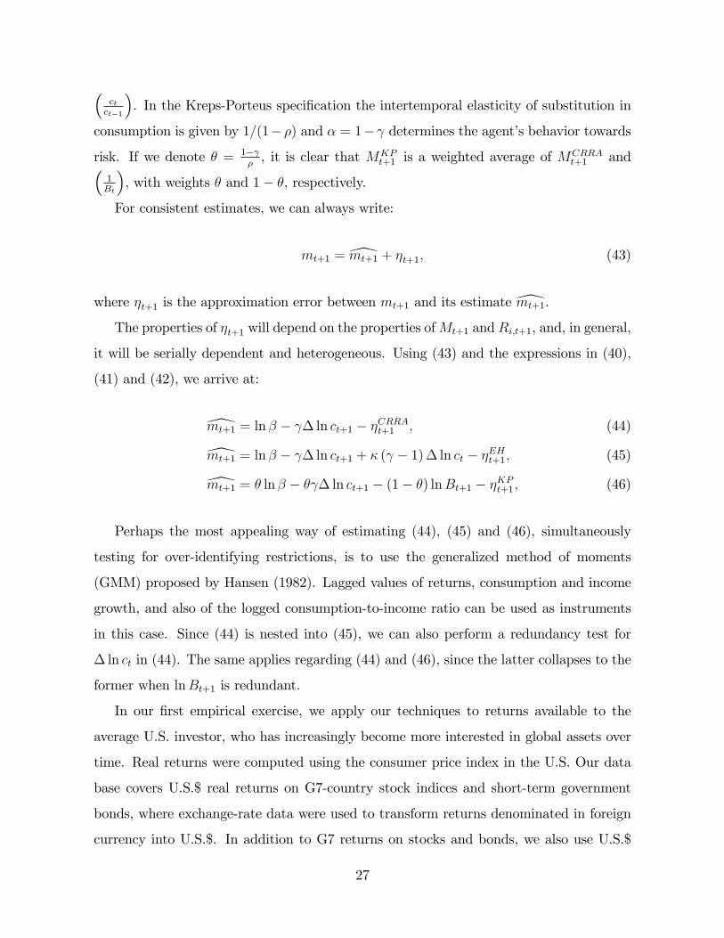
Results using the Kreps-Porteus specification are reported in Table 3. To implement its
31
estimation a first step is to find a proxy to the optimal portfolio. We followed Epstein and
Zin (1991) in choosing the NYSE for that role, although we are aware of the limitations
they raise for this choice. With that caveat, we find that the optimal portfolio term has a
coeffi cient that is close to zero in value (θ close to unity), although (1− θ) is not statically
zero in any regressions we have run. If it were, then the Kreps-Porteus would collapse
to the power-utility specification. The estimates of the relative risk-aversion coeffi cient
are not very similar across regressions, ranging from 0.362 to 1.360. Moreover, they
are not statistically different from zero at the 5% significance level, which differs from
previous estimates in Tables 1 and 2. There is no evidence of rejection in over-identifying
restrictions tests in any GMM regression we have run, which is in sharp contrast to the
early results of Epstein and Zin using this same specification.
Since the Kreps-Porteus encompasses the power utility specification, the former should
be preferred to the latter in principle because (1− θ) is not statistically zero. A reason
against it is the limitation in choosing a proxy for the optimal portfolio. Therefore, the
picture that emerges from the analysis of Tables 1, 2 and 3 is that both the power-utility
and the Kreps-Porteus specifications fit the CCAPM reasonably well when our estimator
of the SDF is employed in estimation. Since κ is statistically zero, we find little evidence
in favor of external habit formation using our data.
3.2 Out-of-Sample Asset-Pricing Forecasting Exercise
Next, we present the results of an asset-pricing out-of-sample forecasting exercise in the
panel-data dimension. In constructing our estimator of the SDF, we try to approxi-
mate the asymptotic environment with monthly U.S. time-series return data from 1980:1
through 2007:12 (T = 336 observations), collected for N = 16, 193 assets, grouped in
the following four categories: mutual funds (7, 932), stocks (6, 009), real estate (383),
and government bonds (1, 869). After computing Mt, we price individual return data not
used in constructing it, measuring the distance between forecast prices and 1 using the δ
pricing-error measure proposed in Hansen and Jagannathan (1997).
All return data used in this exercise come from CRSP. Mutual-Fund return data
32

comes from the CRSP Mutual Fund Database, which reports open-ended mutual-fund
returns using survivor-bias-free data. Bias can arise, for example, when a older fund
splits into other share classes, each new share class being permitted to inherit the entire
return/performance history of the older fund. Stock return data comes from the CRSP
U.S. Stock and CRSP U.S. Indices, which collects returns from NYSE, AMEX, NASDAQ,
and, more recently, NYSE Arca. Real-Estate return data comes from the CRSP/Ziman
Real Estate Data Series. It collects return data on real-estate investment trusts (REITs)
that have traded on the NYSE, AMEX and NASDAQ exchanges. Finally, government-
bond return data comes from CRSP Monthly Treasury U.S. Database, which collects
monthly returns of U.S. Treasury bonds with different maturities.
The first step to perform our exercise is computing Mt. Since we do not have a random
sample of returns, we decided to work with each of the four categories above, weighting
them by their respective importance in the median U.S. household portfolio. For each of
the four asset categories (mutual funds, stocks, real estate, and government bonds) we
computed the geometric average of the reciprocal of all asset returns and the arithmetic
average of all asset returns. Based on the “Wealth and Asset Ownership”tables of 2004,
provided by the U.S. Census Bureau, we decided to weight the returns in each of the
four categories as follows: Mutual Funds (10%), Stocks (10%), Real Estate (60%), and
Government Bonds (20%)8. They are a close approximation of the median (and also the
mean) value of assets owned by U.S. households in these four categories. Local changes
in these weights (from 5 up to 20 percentage points for individual categories) produce no
virtual change on the results of our exercise. Our final estimate Mt results from weighting
geometric and arithmetic averages of returns in each of these four categories.
Once we obtain Mt, we forecast a group of returns not included in computing it for
all the 336 observations in the time-series dimension, comparing our results with unity.
Under the law of one price this exercise is similar in spirit to the one in Hansen and
Jagannathan (1997). Our forecasting exercise is performed using nominal returns either
8These tables can be downloaded from http://www.census.gov/hhes/www/wealth/2004_tables.html.These weights we propose using come from Table 1, which has the “Median Value of Assets for Households,by Type of Asset Owned and Selected Characteristics.”
33

in constructing the SDF or in out-of-sample evaluation of returns. Obviously, the product
MtRi,t is invariant to price inflation as long as the same price index is used in deflating
Mt and Ri,t.
Our estimate of Mt has a nominal mean of 0.9922 in a monthly basis, which amounts
to 0.9106 in a yearly basis. In comparison, average yearly CPI inflation for the same
period is 3.85%. The plot of Mt follows below in Figure 2.
0.92
0.96
1.00
1.04
1.08
1.12
80 82 84 86 88 90 92 94 96 98 00 02 04 06
SDF
Figure 2: Stochastic Discount Factor
We want our forecasting exercise to be out of sample. In choosing the group of assets
which will have their returns priced, we require that they have not been included in com-
puting Mt. To cover a wide spectrum of assets to be priced, we chose to work with stocks,
divided in 10 categories of capitalization, according to the CRSP Stock File Capitaliza-
tion Decile Indices. Their returns are calculated for each of the Stock File Indices market
groups. All securities, excluding ADRs on a given exchange or combination of exchanges,
are ranked according to capitalization and then divided into ten equal parts, each rebal-
34

ancing every year using the security market capitalization at the end of the previous year
to rank securities. The largest securities are placed in portfolio 10 and the smallest in
portfolio 1. Value-Weighted Index Returns including all dividends are calculated on each
of the ten portfolios. Because of the value-weighted character of these portfolios, and the
fact that they are rebalanced every year, their returns cannot be written as a fixed-weight
linear combination of the returns used in computing Mt —therefore do not lie in the space
of returns used in computing Mt. This makes our forecasting exercise out-of-sample in
the panel-data dimension.
We evaluate our estimator Mt in terms of its ability to price the returns of these ten
portfolios divided into capitalization categories. We use the distance measure δ proposed
in Hansen and Jagannathan, which represents the smallest adjustment required in our
estimator to bring it to an admissible SDF. Results are presented in Table 4.
Table 4Out-of-Sample Asset-Pricing Forecast Evaluation
SDF Proxy: Mt
Returns of Capitalization Capitalization CapitalizationPortfolios 1-10 Portfolios 1-5 Portfolios 6-10
Distance Measure δ δ δ(Robust SE) (Robust SE) (Robust SE)0.1493 0.0912 0.0677(0.0483) (0.0442) (0.0589)
Notes: The capitalization portfolios tested in the first three columns come form the CRSPStock File Capitalization Decile Indices. These are divided into 10 capitalization groups, bydecile of capitalization. The largest securities are placed in portfolio 10 and the smallest inportfolio 1. Estimates of the Hansen and Jagannathan distance δ and its respective robuststandard error are computed using the MATLAB code made available by Mike Cliff9. RobustSE are computed using the procedure proposed by Newey and West (1987).
When pricing all 10 capitalization portfolios, the performance of our estimator comes
short of expected. The distance δ is significant at the usual levels of significance. In
trying to understand the reasons for rejecting admissibility, we divided the 10 portfolios
into two groups: “smaller caps,”with deciles of capitalization from 1 to 5, and “larger
caps,”with deciles of capitalization from 6 to 10. In pricing the smaller caps portfolios,
9The code can now be downloaded from:http://sites.google.com/site/mcliffweb/programs
35

δ is still significant at the usual levels, although only marginally so. However, when the
larger caps are priced, our estimator of the SDF is admissible and δ is far from significant;
see also the cross-plot of the required adjustment vs. the SDF value depicted in Figure 3.
Finally, the evidence in Table 4 leads to the conclusion that our initial rejection was
due to misspricing smaller-cap stocks. We do not see this result as a serious drawback for
our estimator. As is well known, there is a much greater volatility in terms of entry and
exit of smaller firms into the marketplace, whose historical positive returns are always
recorded, but some negative results are not recorded due to bankruptcy. Hence, one may
expect some bias in using smaller-cap firms historical returns in asset-pricing tests, which
may be the case here when using capitalization deciles 1 to 5.
0.9 0.95 1 1.05 1.1 1.150.25
0.2
0.15
0.1
0.05
0
0.05
0.1
0.15
0.2
HJ Distance: LOP Kernelδ = 0.0677 se = 0.0589
Candidate (Model) SDF
Adj
ustm
ent t
o M
ake
SD
F V
alid
Figure 3: Admissibility Adjustment vs. SDF Value
36

4 Conclusions
In this paper, we propose a novel consistent estimator for the stochastic discount factor
(SDF), or pricing kernel, that exploits both the time-series and the cross-sectional dimen-
sions of asset prices. We treat the SDF as a random process that can be estimated con-
sistently as the number of time periods and assets in the economy grow without bounds.
To construct our estimator, we basically rely on standard regularity conditions on the
stochastic processes of asset returns and on the absence of arbitrage opportunities in
asset pricing. Our SDF estimator depends exclusively on appropriate averages of asset
returns, which makes its computation a simple and direct exercise. Because it does not
depend on any assumptions on preferences, or on consumption data, we are able to use
our SDF estimator to test directly different preference specifications which are commonly
used in finance and in macroeconomics. We also use it in an out-of-sample asset-pricing
forecasting exercise.
A key feature of our approach is that it combines a general Taylor Expansion of the
Pricing Equation with standard panel-data asymptotic theory to derive a novel consistent
estimator for the SDF. In this context, we show that the econometric identification of the
SDF only requires using the “common-feature property”of the logarithm of the SDF. We
have followed two literature trends here: first, in financial econometrics, recent work avoids
imposing stringent functional-form restrictions on preferences prior to estimation of the
SDF; see Chapman (1998), Aït-Sahalia and Lo (1998, 2000), Rosenberg and Engle (2002),
Garcia, Luger, and Renault (2003), Sentana (2004), Garcia, Renault, and Semenov (2006),
and Sentana, Calzolari, and Fiorentini (2008); second, in macroeconomics, early rejections
of the optimal behavior for consumption using time-series data found by Hall(1978),
Flavin(1981, 1993), Hansen and Singleton(1982, 1983, 1984), Mehra and Prescott(1985),
Campbell (1987), Campbell and Deaton(1989), and Epstein and Zin(1991) were overruled
by subsequent results using panel data by Runkle (1991), Blundell, Browning, and Meghir
(1994), Attanasio and Browning (1995), and Attanasio and Weber (1995), among others.
The techniques discussed in this paper were applied to two relevant issues in macro-
economics and finance: the first asks what type of parametric preference-representation
37

could be valid using our SDF estimator, and the second asks whether or not our SDF
estimator can price returns in an out-of-sample forecasting exercise. In the first appli-
cation, we used quarterly data of U.S.$ real returns from 1972:1 to 2000:4 representing
investment opportunities available to the average U.S. investor. They cover thousands of
assets worldwide, but are predominantly U.S.-based. Our SDF estimator —Mt —is close to
unity most of the time and bounded by the interval [0.85, 1.15], with an equivalent average
annual discount factor of 0.9711, or an annual discount rate of 2.97%. When we examined
the appropriateness of different functional forms to represent preferences, we concluded
that standard preference representations used in finance and in macroeconomics cannot
be rejected by the data. Moreover, estimates of the relative risk-aversion coeffi cient are
close to what can be expected a priori —between 1 and 2, statistically significant and not
different from unity in statistical tests. In the second application, we tried to approxi-
mate the asymptotic environment by working with monthly U.S. time-series return data
from 1980:1 through 2007:12 (T = 336 observations), which were collected for a total of
N = 16, 193 assets. We showed that our SDF proxy can price reasonably well the returns
of stocks with a higher capitalization level, whereas it shows some diffi culty in pricing
stocks with a lower level of capitalization. Because there is more volatility in terms of en-
try and exit of smaller firms into the marketplace, which may generate a bias in historical
returns for “lower cap”returns, rejection in this case may not be too problematic.
References
[1] Abel, A., 1990, “Asset Prices under Habit Formation and Catching Up with the
Joneses,“American Economic Review Papers and Proceedings, 80, 38-42.
[2] Athanasopoulos, G., Guillen, O.T.C., Issler, J.V., and Vahid, F. (2011), “Model
Selection, Estimation and Forecasting in VAR Models with Short-run and Long-run
Restrictions,”forthcoming, Journal of Econometrics.
[3] Attanasio, O., and M. Browning, 1995, “Consumption over the Life Cycle and over
the Business Cycle,”American Economic Review, vol. 85(5), pp. 1118-1137.
38

[4] Attanasio, O., and G. Weber, 1995, “Is Consumption Growth Consistent with In-
tertemporal Optimization? Evidence from the Consumer Expenditure Survey,”Jour-
nal of Political Economy, vol. 103(6), pp. 1121-1157.
[5] Bai, J. and Serena Ng, 2004, “Evaluating Latent and Observed Factors in Macroeco-
nomics and Finance,”Working Paper: University of Michigan.
[6] Blundell, Richard, Martin Browning, and Costas Meghir, 1994, “Consumer Demand
and the Life-Cycle Allocation of Household Expenditures,”Review of Economic Stud-
ies, Vol. 61, No. 1, pp. 57-80 .
[7] Bollerslev, T., Engle, R.F. and Wooldridge, J., 1988, “A Capital Asset Pricing Model
with Time Varying Covariances”, Journal of Political Economy, vol. 96, pp.116-131.
[8] Brown, D.P. and Gibbons, M.R. (1985). “A Simple Econometric Approach for Utility-
based Asset Pricing Models,”Journal of Finance, 40(2): 359-81.
[9] Campbell, J.Y. (1987), “Does Saving Anticipate Declining Labor Income? An Al-
ternative Test of the Permanent Income Hypothesis,”Econometrica, vol. 55(6), pp.
1249-73.
[10] Campbell, J.Y. and Deaton, A. (1989), “Why is Consumption so Smooth?”. Review
of Economic Studies, 56:357-374.
[11] Campbell, J.Y. and Mankiw, G. (1989), “Consumption, Income and Interest Rates:
Reinterpreting the Time Series Evidence”, NBER Macroeconomics Annual, 4:185-
216.
[12] Chapman, David A. (1997), “Approximating the asset pricing kernel”, Journal of
Finance, Vol. 52, pp. 1383-1410.
[13] Christensen, J.H.E., Diebold, F.X. and Rudebusch, G.D. (2009), "An Arbitrage-Free
Generalized Nelson-Siegel Term Structure Model," The Econometrics Journal, 12,
33-64.
39
[14] Christensen, J.H.E., Diebold, F.X. and Rudebusch, G.D. (2011), "The Affi ne
Arbitrage-Free Class of Nelson-Siegel Term Structure Models," Journal of Econo-
metrics, 164, 4-20.
[15] Cochrane, J.H. (2002). Asset Pricing, Princeton and Oxford: Princeton University
Press. Revised Edition.
[16] Diebold, F.X. and Li, C. (2006), "Forecasting the Term Structure of Government
Bond Yields," Journal of Econometrics, 130, 337-364.
[17] Diebold, F.X. and Rudebusch, G.D. (2013), Yield Curve Modeling and Forecast-
ing: The Dynamic Nelson-Siegel Approach (The Econometrics Institute / Tinbergen
Instiitute Lectures). Princeton: Princeton University Press.
[18] Engle, R.F. (1982), “Autoregressive Conditional Heteroskedasticity with Estimates
of the Variance of United Kingdom Inflation,”Econometrica, 50, pp. 987-1006.
[19] Engle, R. F., Issler, J. V., 1995, “Estimating common sectoral cycles,” Journal of
Monetary Economics, vol. 35, 83—113.
[20] Engle, R.F. and Kozicki, S. (1993). “Testing for Common Features”, Journal of
Business and Economic Statistics, 11(4): 369-80.
[21] Engle, R. and Marcucci, J. (2006), “A long-run Pure Variance Common Features
model for the common volatilities of the Dow Jones,”Journal of Econometrics, Vol-
ume 132(1), pp. 7-42.
[22] Epstein, L. and S. Zin, 1991, “Substitution, Risk Aversion, and the Temporal Be-
havior of Consumption and Asset Returns: An Empirical Investigation,”Journal of
Political Economy, 99, 263-286.
[23] Fama, E.F. and French, K.R. (1992).”The Cross-Section of Expected Stock Returns”.
Journal of Finance, 47(2): 427-65.
[24] Fama, E.F. and French, K.R. (1993). “Common Risk Factors in the Returns on Stock
and Bonds”. Journal of Financial Economics, 33(1): 3-56.
40
[25] Flavin, M. (1981), “The Adjustment of Consumption to Changing Expectations
About Future Income”. Journal of Political Economy, 89(5):974-1009.
[26] Forni, M., Hallin, M., Lippi, M. and Reichlin, L. (2000), “The Generalized Dynamic
Factor Model: Identification and Estimation”, Review of Economics and Statistics,
2000, vol. 82, issue 4, pp. 540-554.
[27] Garcia, René, and Eric Renault, 2001, “Latent Variables Models for Stochastic Dis-
count Factors”, in Handbook of Mathematical Finance, E. Jouini, J. Cvitanic and M.
Musiela (Eds.), Cambridge University Press, pp. 159-184.
[28] Garcia, René, Richard Luger, and Eric Renault, 2003, “Empirical Assessment of an
Intertemporal Option Pricing Model with Latent Variables”, Journal of Economet-
rics, 116, pp. 49-83.
[29] Garcia, René, Eric Renault, and Andrei Semenov, 2006, “Disentangling Risk Aver-
sion and Intertemporal Substitution Through a Reference Utility Level.” Finance
Research Letters 3:181, 193.
[30] Geweke, J. (1977), “The Dynamic Factor Analysis of Economic Time Series,”Chapter
19 in D.J. Aigner and A.S. Goldberger (eds.) Latent Variables in Socio-Economic
Models, Amsterdam: North Holland.
[31] Hall, R. (1978), “Stochastic Implications of the Life Cycle Permanent Income Hy-
pothesis: Theory and Evidence”. Journal of Political Economy, 86(6), 971-987.
[32] Hansen, L., 1982, “Large Sample Properties of Generalized Method of Moments
Estimators,”Econometrica, 50, 1029-1054.
[33] Hansen, L. P. and Jagannathan, R. (1991), “Implications of Security Market Data
for Models of Dynamic Economies”, Journal of Political Economy, 99(2):225-262.
[34] Hansen, L. P. and Jagannathan, R. (1997), “Assessing Specification Errors in Sto-
chastic Discount Factor Models.”Journal of Finance, 1997, 52(2), pp. 557-590.
[35] Hansen, Lars Peter and Eric Renault (2009), “Pricing Kernels and Stochastic Dis-
count Factors,”forthcoming in the Encyclopedia of Quantitative Finance.
41

[36] Hansen, L.P. and Scott F. Richard, 1987, “The role of conditioning information in de-
ducing testable restrictions implied by dynamic asset pricing models,”Econometrica,
55:587-613.
[37] Hansen, Lars Peter and José A. Scheinkman (2009), “Long-Term Risk: An Operator
Approach,”Econometrica, 77(1), pp. 177 - 234.
[38] Hansen, L. and K. Singleton, 1982,“Generalized Instrumental Variables Estimation
of Nonlinear Expectations Models,”Econometrica, 50(5), pp. 1269-1286.
[39] Hansen, L. and Singleton, K. (1983), “Stochastic Consumption, Risk Aversion and
the Temporal Behavior of Asset Returns”. Journal of Political Economy, 91(2):249-
265.
[40] Hansen, L. and K. Singleton, 1984, Erratum of the article “Generalized Instrumental
Variables Estimation of Nonlinear Expectations Models,”Econometrica, 52(1), pp.
267-268.
[41] Harrison, J.M. and Kreps, D.M. (1979), “Martingales and arbitrage in multiperiod
securities markets”. Journal of Economic Theory, 20, 381—405.
[42] Hecq, A., Palm, F.C., Urbain, J.-P., 2006, “Testing for common cyclical features
in VAR models with cointegration,” Journal of Econometrics, Volume 132(1), pp.
117-141.
[43] Issler, J. V., Vahid, F., 2001, “Common cycles and the importance of transitory
shocks to macroeconomic aggregates,”Journal of Monetary Economics, vol. 47, 449—
475.
[44] Issler, J.V. and Vahid, F. (2006), “The Missing Link: Using the NBER Recession In-
dicator to Construct Coincident and Leading Indices of Economic Activity,”Journal
of Econometrics, vol. 132(1), pp. 281-303.
[45] Issler, J.V. and Lima, L.R. (2009), “A Panel-Data Approach to Economic Forecast-
ing: The Bias-Corrected Average Forecast,” Journal of Econometrics, Vol. 152(2),
pp. 153-164.
42

[46] Kreps, D. and E. Porteus, 1978, “Temporal Resolution of Uncertainty and Dynamic
Choice Theory,”Econometrica, 46, 185-200.
[47] Lawley, D. N. and Maxwell, A. E. (1971), “Factor Analysis as a Statistical Method.”
Second edition. London: Butterworths.
[48] Lettau, M. and Ludvigson, S. (2001). “Resurrecting the (C)CAPM: A Cross-Sectional
Test When Risk Premia Are Time-Varying,”Journal of Political Economy, 109(6):
1238-87.
[49] Mehra, R., and Prescott, E., 1985, “The Equity Premium: A Puzzle,” Journal of
Monetary Economics, 15, 145-161.
[50] Mulligan, C. (2002), “Capital, Interest, and Aggregate Intertemporal Substitution,”
Working Paper # w9373: National Bureau of Economic Research.
[51] Newey, W. K., West, K. D., 1987, “A simple, positive semi-definite, heteroskedasticity
and autocorrelation consistent covariance matrix,”Econometrica, vol. 55, 703—708.
[52] Rosenberg, J. and Engle, R.F. (2002), “Empirical Pricing Kernels”, Journal of Fi-
nancial Economics, Vol. 64, 3, pp. 341-372.
[53] Ross, S.A. (1976), “The arbitrage pricing of capital asset pricing”, Journal of Eco-
nomic Theory, 13, pp. 341-360.
[54] Runkle, D. (1991), “Liquidity Constraints and the Permanent Income Hypothesis:
Evidence from Panel Data”. Journal of Monetary Economics, 27(1):73-98.
[55] Sentana, Enrique, 2004, “Factor representing portfolios in large asset markets,”Jour-
nal of Econometrics, Volume 119, Issue 2, pp. 257-289.
[56] Sentana, Enrique, Giorgio Calzolari, Gabriele Fiorentini, 2008, “Indirect estimation
of large conditionally heteroskedastic factor models, with an application to the Dow
30 stocks,”Journal of Econometrics, Volume 146, Issue 1, pp. 10-25.
[57] Sentana, Enrique, Gabriele Fiorentini, 2001, Identification, estimation and testing of
conditionally heteroskedastic factor models, Journal of Econometrics, Volume 102,
Issue 2, pp. 143-164.
43

[58] Stock, J. and Watson, M. (1989) “New Indexes of Leading and Coincident Economic
Indicators”, NBER Macroeconomics Annual, pp. 351-95.
[59] Stock, J. andWatson, M. (1993), Eds., “New Research on Business Cycles, Indicators
and Forecasting”Chicago: University of Chicago Press, for NBER.
[60] Stock, J. and Watson, M. (2002) “Forecasting Using Principal Components From a
Large Number of Predictors,”Journal of the American Statistical Association, Vol.
97, pp. 1167-1179.
[61] Vahid, F. and Engle, R. F., 1993, “Common trends and common cycles,”Journal of
Applied Econometrics, vol. 8, 341—360.
[62] Vahid, F., Engle, R. F., 1997, “Codependent cycles,”Journal of Econometrics, vol.
80, 199—221.
[63] Vahid, F., Issler, J. V., 2002, “The importance of common cyclical features in VAR
analysis: A Monte Carlo study,”Journal of Econometrics, 109, 341—363.
44


![GSA - Microsoft...6.Discount from list prices: 52.64% Discount off Commercial List [0.4736 factor] 7.Quantity discounts: (based on total net price) $10,001 - $25,000 55.01% Discount](https://img.pdfslide.us/doc/110x75/601c4243cfcb20377c048115/gsa-microsoft-6discount-from-list-prices-5264-discount-off-commercial.jpg)