A BODY-EXACT STRIP THEORY APPROACHTO SHIP MOTION COMPUTATIONS
by
Piotr Jozef Bandyk
A dissertation submitted in partial fulfillmentof the requirements for the degree of
Doctor of Philosophy(Naval Architecture and Marine Engineering)
in The University of Michigan2009
Doctoral Committee:
Professor Robert F. Beck, ChairProfessor Smadar KarniProfessor Armin W. TroeschAssociate Reseach Scientist Okey Nwogu

c© Piotr Jozef Bandyk 2009
All Rights Reserved
ACKNOWLEDGEMENTS
I would like to give a special thanks to Prof. Beck for being my thesis adviser
and a great friend. From early on as an undergraduate in his courses, to the days
when we would spend hours discussing research, his vast insight, attention to detail,
and guidance have made this dissertation possible. A very special thanks to my
committee members, Dr. Nwogu, Prof. Troesch, and Prof. Karni, for their individual
contributions to my education and helpful discussions about research.
I also want to thank my family, especially my parents, Jerzy and Maria Bandyk, for
their continuous support, encouragement, and understanding throughout my entire
academic career. From a home-cooked meal, to helping with work around the car, it
makes life is a little more enjoyable and less stressful.
I want to thank my friends, in and outside school, for being there when I needed
them and being patient with me when research required all of my attention. I would
especially like to thank my colleagues and office-mates, Jim Bretl, Ellie Nick, and
Chris Hart, for countless meaningful conversations, whether they be about schoolwork
or not.
I want to thank the Naval Architecture and Marine Engineering department fac-
ulty and staff for providing an excellent environment for learning and helping with
funding along the way. My continuous career from undergraduate to graduate school
is a testament to their dedication to the students.
This dissertation was primarily funded by the Office of Naval Research and it is
gratefully acknowledged.
ii

TABLE OF CONTENTS
ACKNOWLEDGEMENTS . . . . . . . . . . . . . . . . . . . . . . . . . . ii
LIST OF FIGURES . . . . . . . . . . . . . . . . . . . . . . . . . . . . . . . v
LIST OF TABLES . . . . . . . . . . . . . . . . . . . . . . . . . . . . . . . . ix
LIST OF APPENDICES . . . . . . . . . . . . . . . . . . . . . . . . . . . . x
ABSTRACT . . . . . . . . . . . . . . . . . . . . . . . . . . . . . . . . . . . xi
CHAPTER
I. Introduction . . . . . . . . . . . . . . . . . . . . . . . . . . . . . . 1
1.1 Background . . . . . . . . . . . . . . . . . . . . . . . . . . . . 11.2 Overview . . . . . . . . . . . . . . . . . . . . . . . . . . . . . 5
II. Problem Formulation . . . . . . . . . . . . . . . . . . . . . . . . . 7
2.1 Conventions and Coordinate Systems . . . . . . . . . . . . . . 72.2 The Governing Equations . . . . . . . . . . . . . . . . . . . . 92.3 Strip Theory Approximation . . . . . . . . . . . . . . . . . . 122.4 Boundary Integral Method . . . . . . . . . . . . . . . . . . . 152.5 Velocity Potential Decomposition . . . . . . . . . . . . . . . . 162.6 Mixed Boundary Value Problem . . . . . . . . . . . . . . . . 172.7 Forces and Moments . . . . . . . . . . . . . . . . . . . . . . . 202.8 Equations of Motion . . . . . . . . . . . . . . . . . . . . . . . 212.9 The Acceleration Potential . . . . . . . . . . . . . . . . . . . 232.10 Viscous Forces . . . . . . . . . . . . . . . . . . . . . . . . . . 27
III. Numerical Techniques . . . . . . . . . . . . . . . . . . . . . . . . 31
3.1 Source Distribution Method . . . . . . . . . . . . . . . . . . . 313.2 Domain Discretization . . . . . . . . . . . . . . . . . . . . . . 34
iii
3.3 Time-Stepping . . . . . . . . . . . . . . . . . . . . . . . . . . 363.4 Body and Free Surface Intersection . . . . . . . . . . . . . . . 373.5 Section Exit and Entry . . . . . . . . . . . . . . . . . . . . . 383.6 Radial Basis Functions . . . . . . . . . . . . . . . . . . . . . . 393.7 Computation Time . . . . . . . . . . . . . . . . . . . . . . . . 43
IV. Two-Dimensional Results . . . . . . . . . . . . . . . . . . . . . . 45
4.1 Validation of the Acceleration Potential . . . . . . . . . . . . 454.2 Convergence Studies . . . . . . . . . . . . . . . . . . . . . . . 484.3 Small Amplitude Radiation . . . . . . . . . . . . . . . . . . . 524.4 Large Amplitude Oscillations of a Circular Cylinder . . . . . 55
V. Strip Theory Results . . . . . . . . . . . . . . . . . . . . . . . . . 63
5.1 Small Amplitude Radiation . . . . . . . . . . . . . . . . . . . 645.2 Wave Exciting Forces . . . . . . . . . . . . . . . . . . . . . . 715.3 Large Amplitude Radiation . . . . . . . . . . . . . . . . . . . 71
VI. Free Motions . . . . . . . . . . . . . . . . . . . . . . . . . . . . . . 80
6.1 Nonlinear Equations of Motion . . . . . . . . . . . . . . . . . 80
VII. Discussion . . . . . . . . . . . . . . . . . . . . . . . . . . . . . . . . 89
7.1 Conclusions . . . . . . . . . . . . . . . . . . . . . . . . . . . . 897.2 Recommendations . . . . . . . . . . . . . . . . . . . . . . . . 90
APPENDICES . . . . . . . . . . . . . . . . . . . . . . . . . . . . . . . . . . 92
BIBLIOGRAPHY . . . . . . . . . . . . . . . . . . . . . . . . . . . . . . . . 117
iv
LIST OF FIGURES
Figure
2.1 Coordinate Systems . . . . . . . . . . . . . . . . . . . . . . . . . . . 8
2.2 Two-Dimensional Boundary Value Problem . . . . . . . . . . . . . . 19
3.1 RBF cj comparison, φ ∝ x2 . . . . . . . . . . . . . . . . . . . . . . . 41
3.2 RBF cj comparison, φ ∝ x2 + x3 . . . . . . . . . . . . . . . . . . . . 41
4.1 Circular Cylinder Forced Heave, a = 2m, R = 10m, ω2R/g = 1.5 . . 46
4.2 Circular Cylinder Forced Heave, a = 4m, R = 10m, ω2R/g = 1.5 . . 47
4.3 Circular Cylinder Forced Heave, a = 6m, R = 10m, ω2R/g = 1.5 . . 47
4.4 Convergence of Circular Cylinder in Heave, ω = 0.6 . . . . . . . . . 50
4.5 Convergence of Circular Cylinder in Heave, ω = 1.6 . . . . . . . . . 51
4.6 Circular Cylinder Heave Added Mass and Damping . . . . . . . . . 53
4.7 Circular Cylinder Sway Added Mass and Damping . . . . . . . . . . 54
4.8 Box Barge Heave Added Mass and Damping . . . . . . . . . . . . . 56
4.9 Box Barge Sway Added Mass and Damping . . . . . . . . . . . . . 57
4.10 Box Barge Roll Added Mass and Damping . . . . . . . . . . . . . . 58
4.11 Box Barge Roll-Sway Added Mass and Damping . . . . . . . . . . . 59
4.12 Box Barge Sway-Roll Added Mass and Damping . . . . . . . . . . . 60
v

5.1 Wigley I Heave Hydrodynamic Coefficients, Fn = 0.3 . . . . . . . . 66
5.2 Wigley I Pitch Hydrodynamic Coefficients, Fn = 0.3 . . . . . . . . 67
5.3 Wigley I Pitch-Heave Hydrodynamic Coefficients, Fn = 0.3 . . . . . 67
5.4 Wigley I Heave-Pitch Hydrodynamic Coefficients, Fn = 0.3 . . . . . 68
5.5 Wigley III Heave Hydrodynamic Coefficients, Fn = 0.3 . . . . . . . 69
5.6 Wigley III Pitch Hydrodynamic Coefficients, Fn = 0.3 . . . . . . . 69
5.7 Wigley III Pitch-Heave Hydrodynamic Coefficients, Fn = 0.3 . . . . 70
5.8 Wigley III Heave-Pitch Hydrodynamic Coefficients, Fn = 0.3 . . . . 70
5.9 Wigley I Heave Exciting Force in Head Seas, Fn = 0.3 . . . . . . . 72
5.10 Wigley I Pitch Exciting Moment in Head Seas, Fn = 0.3 . . . . . . 72
5.11 Views of m5514 (Naval Destroyer) Hull . . . . . . . . . . . . . . . . 73
5.12 m5514 Forced Pitch, ω = 0.3831rad/s . . . . . . . . . . . . . . . . . 75
5.13 m5514 Forced Pitch, ω = 1.1000rad/s . . . . . . . . . . . . . . . . . 75
5.14 m5514 Forced Pitch (Backward Diff), ω = 0.3831rad/s . . . . . . . 76
5.15 m5514 Forced Pitch (Backward Diff), ω = 1.1000rad/s . . . . . . . 76
5.16 Views of m5613 (ONR Tumblehome) Hull . . . . . . . . . . . . . . 78
5.17 m5613 Forced Pitch, ω = 0.3831rad/s . . . . . . . . . . . . . . . . . 79
5.18 m5613 Forced Pitch, ω = 1.1000rad/s . . . . . . . . . . . . . . . . . 79
6.1 Series-60 (CB=0.7) Heave RAO in Head Seas, Fn = 0.2 . . . . . . . 81
6.2 Series-60 (CB=0.7) Pitch RAO in Head Seas, Fn = 0.2 . . . . . . . 82
6.3 S-175 Surge RAO in Head Seas . . . . . . . . . . . . . . . . . . . . 83
6.4 S-175 Heave RAO in Head Seas . . . . . . . . . . . . . . . . . . . . 84
6.5 S-175 Pitch RAO in Head Seas . . . . . . . . . . . . . . . . . . . . . 84
vi

6.6 S-175 Surge RAO in Stern Quartering Seas . . . . . . . . . . . . . . 85
6.7 S-175 Sway RAO in Stern Quartering Seas . . . . . . . . . . . . . . 86
6.8 S-175 Heave RAO in Stern Quartering Seas . . . . . . . . . . . . . . 86
6.9 S-175 Roll RAO in Stern Quartering Seas . . . . . . . . . . . . . . . 87
6.10 S-175 Pitch RAO in Stern Quartering Seas . . . . . . . . . . . . . . 87
6.11 S-175 Yaw RAO in Stern Quartering Seas . . . . . . . . . . . . . . . 88
A.1 Pressure and Momentum Comparison - Large Amplitude HeavingCircular Section . . . . . . . . . . . . . . . . . . . . . . . . . . . . . 95
A.2 Pressure and Momentum Comparison - Heaving Circular Section at1.0m Amplitude . . . . . . . . . . . . . . . . . . . . . . . . . . . . . 96
A.3 Pressure and Momentum Comparison - Heaving Circular Section at4.0m Amplitude . . . . . . . . . . . . . . . . . . . . . . . . . . . . . 96
A.4 Pressure and Momentum Comparison - Heaving Circular Section at7.0m Amplitude . . . . . . . . . . . . . . . . . . . . . . . . . . . . . 97
B.1 Parameterization of panel integrals using t, the tangent variable . . 101
C.1 φ on Body, Deeply Submerged Heaving Circular Cylinder . . . . . . 104
C.2 φy, φz on Body, Deeply Submerged Heaving Circular Cylinder . . . 104
C.3 φyy, φyz on Body, Deeply Submerged Heaving Circular Cylinder . . . 105
C.4 φyy, φyz Comparison at Field Points in Fluid Domain, in Radial Di-rection from Body, Panel Length dl = 0.042R . . . . . . . . . . . . . 106
C.5 Corrected φyy, φyz on Body . . . . . . . . . . . . . . . . . . . . . . . 107
D.1 S-175 Surge RAO in Following Seas . . . . . . . . . . . . . . . . . . 109
D.2 S-175 Heave RAO in Following Seas . . . . . . . . . . . . . . . . . . 109
D.3 S-175 Pitch RAO in Following Seas . . . . . . . . . . . . . . . . . . 110
D.4 S-175 Surge RAO in Beam Seas . . . . . . . . . . . . . . . . . . . . 110
vii

D.5 S-175 Sway RAO in Beam Seas . . . . . . . . . . . . . . . . . . . . 111
D.6 S-175 Heave RAO in Beam Seas . . . . . . . . . . . . . . . . . . . . 111
D.7 S-175 Roll RAO in Beam Seas . . . . . . . . . . . . . . . . . . . . . 112
D.8 S-175 Pitch RAO in Beam Seas . . . . . . . . . . . . . . . . . . . . 112
D.9 S-175 Yaw RAO in Beam Seas . . . . . . . . . . . . . . . . . . . . . 113
D.10 S-175 Surge RAO in Bow Quartering Seas . . . . . . . . . . . . . . 113
D.11 S-175 Sway RAO in Bow Quartering Seas . . . . . . . . . . . . . . . 114
D.12 S-175 Heave RAO in Bow Quartering Seas . . . . . . . . . . . . . . 114
D.13 S-175 Roll RAO in Bow Quartering Seas . . . . . . . . . . . . . . . 115
D.14 S-175 Pitch RAO in Bow Quartering Seas . . . . . . . . . . . . . . . 115
D.15 S-175 Yaw RAO in Bow Quartering Seas . . . . . . . . . . . . . . . 116
viii
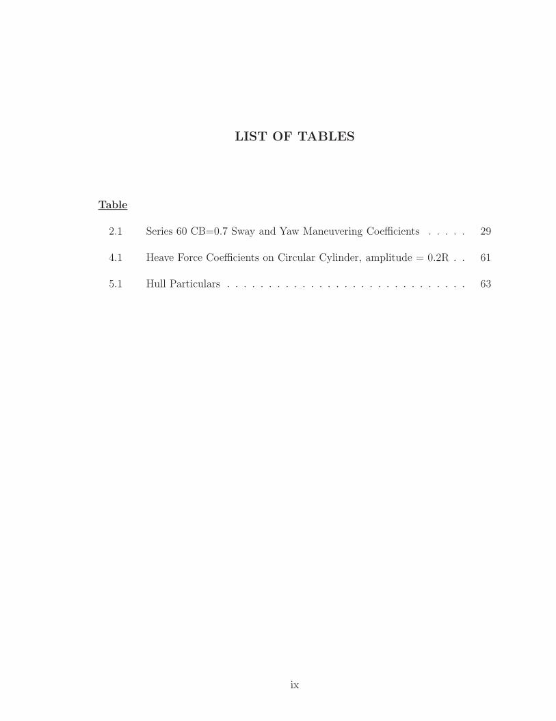
LIST OF TABLES
Table
2.1 Series 60 CB=0.7 Sway and Yaw Maneuvering Coefficients . . . . . 29
4.1 Heave Force Coefficients on Circular Cylinder, amplitude = 0.2R . . 61
5.1 Hull Particulars . . . . . . . . . . . . . . . . . . . . . . . . . . . . . 63
ix
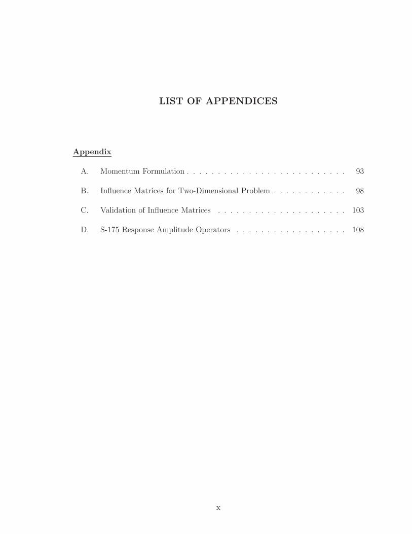
LIST OF APPENDICES
Appendix
A. Momentum Formulation . . . . . . . . . . . . . . . . . . . . . . . . . . 93
B. Influence Matrices for Two-Dimensional Problem . . . . . . . . . . . . 98
C. Validation of Influence Matrices . . . . . . . . . . . . . . . . . . . . . 103
D. S-175 Response Amplitude Operators . . . . . . . . . . . . . . . . . . 108
x
ABSTRACT
A BODY-EXACT STRIP THEORY APPROACH TO SHIP MOTIONCOMPUTATIONS
by
Piotr Jozef Bandyk
Chair: Robert F. Beck
A body-exact strip theory is developed to solve nonlinear ship motion problems
in the time-domain. The hydrodynamic model uses linearized free surface conditions
for computational efficiency and stability, and exact body boundary conditions to
capture events such as slamming and submergence. The strip theory approach is used
to speed up computations and reduce the difficulty in modeling complex geometries.
A nonlinear rigid body equation of motion solver is coupled to the hydrodynamic
model to predict ship responses in large waves.
Constant source strength flat panels are used to model the body and desingularized
sources are used on the free surface. At each time-step, a mixed boundary value
problem is solved. The free surface and rigid body motions are evolved using a fourth-
order Adams-Bashforth time-stepping technique. The acceleration potential is used
to increase numerical accuracy and highlight the coupling between the hydrodynamic
and rigid body motion problems, improving stability.
The problem formulation is comprehensive, and details of numerical techniques are
xi
included. Two-dimensional problems are used to study the accuracy and convergence
of the method. Strip theory results include a variety of hull forms: two Wigley
models (I and III), a Series-60 hull, the ITTC standard S-175 containership, and two
naval vessels. This emphasizes the robust capabilities of the method and presents
a variety of analyses for discussion. The two-dimensional and strip theory results
include small and large amplitude motions. Comparisons to experiments and other
numerical methods are shown and discussed, when possible. In several cases, a variety
of alternative solution techniques are shown to highlight improvements or differences
in problem formulation.
The results obtained show good agreement with previous computational and ex-
perimental results. The method developed is accurate, robust, very computationally
efficient, and can predict nonlinear ship motions. It is well suited to be used as a tool
in ship design or as part of a path optimization model.
xii

CHAPTER I
Introduction
There are various aspects to ship design, such as strength, stability, resistance
and propulsion, seakeeping, maneuvering and controls. Tools and techniques are
available to assess the qualities or characteristics of these components, but very few
of them overlap and take other components into consideration. There are “total”
design packages which estimate all of these aspects at the most primitive level and
offer a well-balanced design. In certain cases, it is perhaps unnecessary or impractical
to delve too deeply into how these pieces of ship design fit together and influence
one another. However, certain relationships can not be treated independently. In
particular, the seakeeping performance of a ship will have significant impact on the
rest of the design.
Linear strip theory can provide quick answers for preliminary design, but is unable
to predict behavior for extreme events which are often of interest. The goal of this
dissertation is to formulate an approach that can predict nonlinear events while being
computationally efficient and robust. This approach can then be used in the design
stage or for real-time simulations to predict vessel loading and responses.
1.1 Background
Wehausen and Laitone (1960) give a detailed overview of various analytical meth-
1

ods for fluid problems. The governing equations and certain ideas have remained
unchanged, such as the use of potential flow theory. The boundary element method
is the most common technique to solve these problems. However, the implementation
of the ideas has been evolving.
Modern seakeeping computations date back to the 1950’s. Korvin-Kroukovsky
and Jacobs (1957) discuss a slender-body approach to model heave and pitch motions.
Gerritsma and Beukelman (1967) validated a strip theory with experimental results.
These resulted in one of the most significant developments, the classical strip theory
by Salvesen et al. (1970), including forward speed effects using the methods derived by
Ogilvie and Tuck (1969). They extended the frequency-domain strip theory approach
to five degrees-of-freedom. The surge degree-of-freedom was added in a consistent
manner by Beck (1989).
Several attempts were made to combine the low-frequency slender-body theory
with the high-frequency strip theory. The unified theory of Newman (1978) and the
asymptotic matching method of Yeung and Kim (1985) are just two examples.
These frequency-domain methods are used extensively for linear calculations and
are very satisfactory for small amplitudes. In order to capture nonlinearities, more
work must be done. The increase in computational power has made it feasible to solve
the viscous problem in the time-domain, as is done in unsteady Reynolds-Averaged
Navier-Stokes (RANS) codes. The computational effort perhaps outweighs the results,
even on modern computers. A one-minute time history of a ship in a seaway may
take hundreds or thousands of CPU hours to simulate.
The time-domain approach has been applied to the potential flow theory for com-
putational efficiency and capturing of nonlinear effects. The Mixed Euler-Lagrange
(MEL) approach was developed by Longuet-Higgins and Cokelet (1976), solving the
fully nonlinear two-dimensional water wave problem. MEL methods have been used
to solve the fully nonlinear three-dimensioanl wave and wave-body interactions, Cao
2
et al. (1990), Cao (1991), Scorpio et al. (1996). A mixed boundary value problem is
set up by knowing the instantaneous body velocity and free surface elevation. Non-
linear free surface boundary conditions are used to update the wave amplitude and
an equation of motion solver may be used to update the body velocity and position.
Free surface instabilities have been found in many cases, and wave breaking may oc-
cur. Techniques to overcome these issues have been proposed, but they are not very
robust. Results of the MEL method are discussed by Beck (1999).
Sclavounos et al. (1997) discuss the developement of SWAN-1 and SWAN-2 based
on the linearized double-body formulation, originally presented by Dawson (1977).
Both codes are three-dimensional. SWAN-1 is linearized about the calm water surface,
while SWAN-2 utilizes the weak scatterer hypothesis by Pawlowski (1992), in which
the ship is assumed to be a weak scatterer whose presence has negligible effects on the
incident and steady wave field. Kring et al. (1996) present results using this approach,
and they appear to be an improvement on motion prediction over linear theory.
The 2D+t approach has been developed by Maruo and Song (1994) and Tulin
and Wu (1996). The two-dimensional flow problem is solved at cross-sections of the
ship. Hyperbolic marching is used in the longitudinal direction, starting at the bow,
to account for the free surface interactions between the two-dimensional sections. A
similar approach was developed by Faltinsen and Zhao (1991). These methods show
significant improvements over strip theory for high-speed ships. The 2D+t methods
may still utilize the fully nonlinear free surface conditions. The difficulty in evolving
the nonlinear free surface is when large amplitude motions cause waves to break.
In potential flow, large amplitude motion problems are most easily dealt with
by using linearized free surface and exact body boundary conditions. This so called
body-exact problem was developed by Beck and Magee (1990) using a time-domain
Green’s function. A similar approach for a surface-piercing body was developed by
Lin and Yue (1990). The variability of wetted surface and hull shape changes due to
3
incident waves and ship motions can be modeled accurately. Beck and Reed (2001)
give a good overview of the state-of-the-art for ship motion computations, describing
some of the methods listed here.
In the simplest case of the body-exact blended method, exact hydrostatics and
Froude-Krylov exciting forces can be combined with linear diffraction and radiation
forces, as the latter two are more expensive to calculate. Finn et al. (2003) present a
strip theory approach where the nonlinear radiation forces are calculated in geomet-
rically complex sections where nonlinearities occur, such as the bow.
Zhang and Beck (2007) discuss two-dimensional large amplitude motions of circu-
lar, box, and wedge shapes. The slamming problem is presented with encouraging re-
sults. Zhang (2007) continues to extend the body-exact approach to three-dimensions
and good results are shown for a Wigley Hull and S-175 Containership when compared
to other codes and experiments. Zhang et al. (2007) extend the two-dimensional code
to a strip theory for arbitrary hull geometries and an extensive comparison is done
between the strip theory and three-dimensional results. The methods compare well,
although the advantages of the strip theory are evident: computation time is an order
of magnitude faster and modeling arbitrary hull geometries is not as complicated.
Fossen (1991) describes the six degree-of-freedom rigid body equations of motions
for underwater and surface marine vehicles. Fossen (2005) uses this approach for non-
linear ship motion predictions. However, the linear frequency-domain hydrodynamic
coefficients are used. Using the time-domain approach, numerical instabilities may
arise in the equations of motion. A possible solution to this is to determine the fluid
acceleration directly. The utilization of the so called “acceleration potential” can be
found in Vinje and Brevig (1981) for the two-dimensional problem, and extended to
three-dimensions by Kang and Gong (1990) and Tanizawa (1995).
The acceleration potential can be used along with the body equations of motion
to improve numerical stability. Examples of this can be seen in Yang (2004) and van
4

Daalen (1993). Most of these methods utilize linear hydrodynamic models. Kang and
Gong (1990) show some interesting nonlinear results for large amplitude motions of
a sphere.
Bishop and Price (1981) presented one of the first comparisons of the seakeep-
ing and maneuvering formulations, in their classical sense. Later, Bailey et al.
(1998) made an attempt at combining seakeeping and maneuvering into a unified
model. They describe some techniques to correct the hydrodynamic coefficients and
account for the viscous characteristics found in maneuvering. Fossen and Smogeli
(2004) describe a combined approach for the equations of motion, linear hydrody-
namics, and viscous maneuvering term corrections. Fang et al. (2005) and Sutulo
and Guedes Soares (2008) describe similar methods to model a ship undergoing a
turning circle in a wave field. In both cases, the hydrodynamic model is based on a
linear strip theory.
1.2 Overview
This dissertation presents the development of a blended method that captures the
nonlinearities of the loads acting on the ship while using linear free surface conditions.
The nonlinear hydrodynamic model is coupled to a nonlinear rigid body equation
of motion solver. Aspects of maneuvering theory may be carefully added to the
seakeeping model to demonstrate how they affect one another. Traditionally, the
seakeeping and maneuvering are treated separately. Care must be taken to account
for the overlap between the high-frequency potential flow seakeeping model and the
low-frequency maneuvering model, where viscous terms are important.
The combination of a body-nonlinear time-domain approach coupled with non-
linear equations of motion and some maneuvering corrections is unique. The strip
theory approximation allows for faster computations and simplified body geometry
definition. The result is a hydrodynamic model that allows the prediction of nonlin-
5

ear loads and motions in a very efficient and robust manner. The theory, numerical
methods, validations, and discussion will be broken up as follows.
Chapter II describes the problem formulation. This includes the conventions used,
explanation and justification of the assumptions made, and description of the bound-
ary conditions. The coupling between the equations of motion and acceleration po-
tential is described in detail.
Chapter III describes the details of the numerical techniques used, including the
discretization of the two-dimensional boundary, time marching and stability, and
treatment of the forward speed terms.
Chapter IV presents the two-dimensional results. This includes convergence stud-
ies, linear validations, and large amplitude validations.
Chapter V presents the strip theory results for prescribed motions. A variety of
hull forms are used to validate the linear hydrodynamic coefficients, exciting forces,
and some discussion of large amplitude motions.
Chapter VI validates the equations of motion using the body-exact hydrodynamic
model. Small wave amplitudes are used to compare the results to the response am-
plitude operators of linear theory.
Chapter VII discusses the contributions of this dissertation and possible consid-
erations for future work.
6
CHAPTER II
Problem Formulation
2.1 Conventions and Coordinate Systems
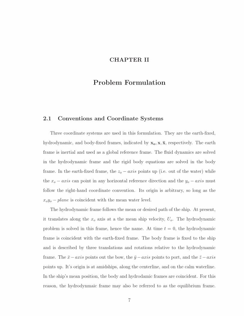
Three coordinate systems are used in this formulation. They are the earth-fixed,
hydrodynamic, and body-fixed frames, indicated by xo,x, x, respectively. The earth
frame is inertial and used as a global reference frame. The fluid dynamics are solved
in the hydrodynamic frame and the rigid body equations are solved in the body
frame. In the earth-fixed frame, the zo − axis points up (i.e. out of the water) while
the xo − axis can point in any horizontal reference direction and the yo − axis must
follow the right-hand coordinate convention. Its origin is arbitrary, so long as the
xoyo − plane is coincident with the mean water level.
The hydrodynamic frame follows the mean or desired path of the ship. At present,
it translates along the xo axis at a the mean ship velocity, Uo. The hydrodynamic
problem is solved in this frame, hence the name. At time t = 0, the hydrodynamic
frame is coincident with the earth-fixed frame. The body frame is fixed to the ship
and is described by three translations and rotations relative to the hydrodynamic
frame. The x−axis points out the bow, the y−axis points to port, and the z−axis
points up. It’s origin is at amidships, along the centerline, and on the calm waterline.
In the ship’s mean position, the body and hydrodamic frames are coincident. For this
reason, the hydrodynmaic frame may also be referred to as the equilibrium frame.
7

xy
z
—x—y
—z
xoyo
zo
Figure 2.1: Coordinate Systems
The relationship of the three frames to one another is illustrated in Figure 2.1
The use of several reference frames requires a clear and consistent statement about
gradients and derivatives. The hydrodynamics and rigid body dynamics are solved
in different frames. Bernoulli’s equation is derived in the hydrodynamic frame, while
the rigid body equations of motion are solved in the body frame.
Three time-derivative conventions are described. The partial ∂, substantial D,
and prescribed path δ time-derivates will be used regularly in the derivation of the
problem. In terms of the velocity potential, the partial time-derivative, ∂φ∂t
, is fixed in
the hydrodynamic frame. This is the same term as appears in Bernoulli’s equation,
as written in the hydrodynamic frame. The other time-derivatives are related by
D
Dt=
∂
∂t+ u · ∇ (2.1)
δ
δt=
∂
∂t+ V · ∇ (2.2)
where u is the fluid velocity and V is a prescribed velocity, all in the hydrodynamic
frame.
8
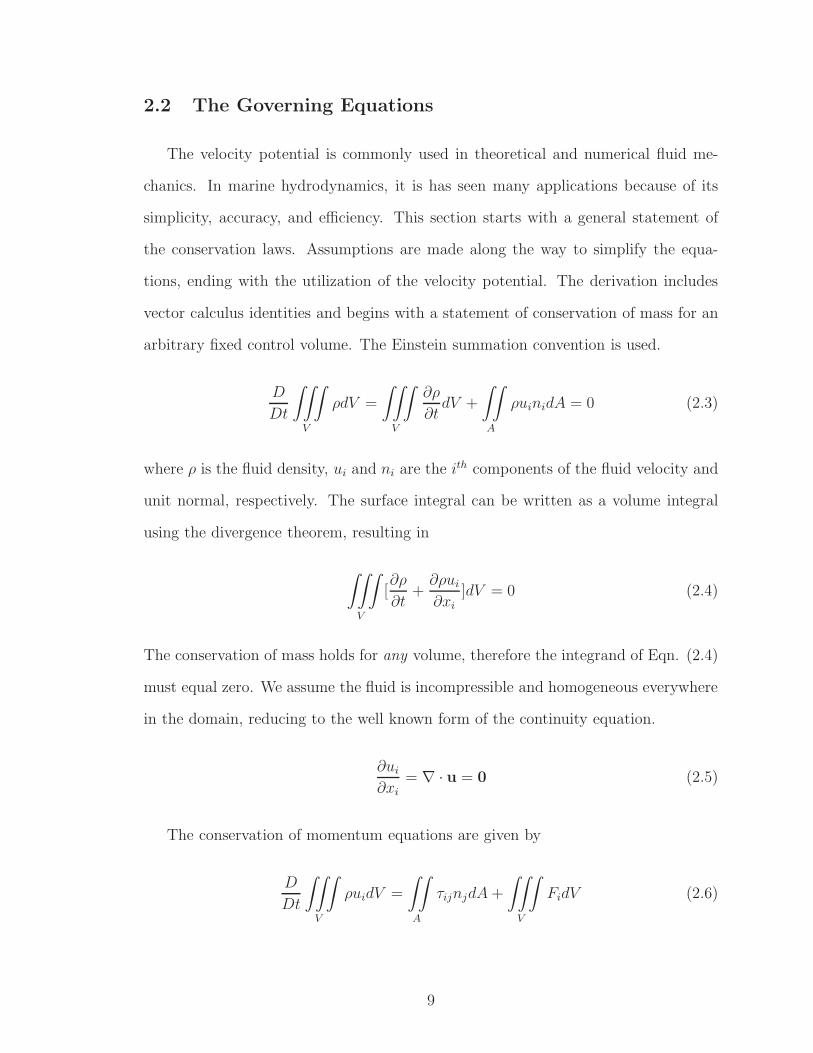
2.2 The Governing Equations
The velocity potential is commonly used in theoretical and numerical fluid me-
chanics. In marine hydrodynamics, it is has seen many applications because of its
simplicity, accuracy, and efficiency. This section starts with a general statement of
the conservation laws. Assumptions are made along the way to simplify the equa-
tions, ending with the utilization of the velocity potential. The derivation includes
vector calculus identities and begins with a statement of conservation of mass for an
arbitrary fixed control volume. The Einstein summation convention is used.
D
Dt
∫∫∫
V
ρdV =
∫∫∫
V
∂ρ
∂tdV +
∫∫
A
ρuinidA = 0 (2.3)
where ρ is the fluid density, ui and ni are the ith components of the fluid velocity and
unit normal, respectively. The surface integral can be written as a volume integral
using the divergence theorem, resulting in
∫∫∫
V
[∂ρ
∂t+∂ρui
∂xi]dV = 0 (2.4)
The conservation of mass holds for any volume, therefore the integrand of Eqn. (2.4)
must equal zero. We assume the fluid is incompressible and homogeneous everywhere
in the domain, reducing to the well known form of the continuity equation.
∂ui
∂xi= ∇ · u = 0 (2.5)
The conservation of momentum equations are given by
D
Dt
∫∫∫
V
ρuidV =
∫∫
A
τijnjdA+
∫∫∫
V
FidV (2.6)
9
where τij is the stress tensor, and Fi is an external force. The surface integral term in
Eqn. (2.6) can be transformed into a volume integral using the divergence theorem.
The left hand side of Eqn. (2.6) can be rewritten similarly to Eqn. (2.4)
∫∫∫
V
[∂ρui
∂t+∂ρuiuj
∂xj
− ∂τij∂xj
− Fi]dV = 0 (2.7)
and since it holds for any volume, the integrand in Eqn. (2.7) must equal zero. The
stress-strain relation for an incompressible Newtonian fluid is given by
τij = −pδij + µ(∂ui
∂xj
+∂uj
∂xi
) (2.8)
where δij is the Kronecker delta function (δij = 1 if i = j, δij = 0 if i 6= j), p is the
pressure, µ is the viscosity of the fluid. This relation can be used to rewrite the third
term in Eqn. (2.7)
∂τij∂xj
= − ∂p
∂xi+ µ
∂2ui
∂xj∂xj(2.9)
The result is a form of the incompressible Navier-Stokes equations, written below
using tensor and vector notation
ρ∂ui
∂t+ ρuj
∂ui
∂xj= − ∂p
∂xi+ µ
∂2ui
∂x2j
+ Fi (2.10)
ρ∂u
∂t+ ρ(u · ∇)u = −∇p + µ∇2u + F (2.11)
Next, we replace the conservative force F with a scalar function Υ = −ρgz, such
that ∇Υ = F. The vorticity is given by Ω = ∇× u and the following vector identity
is used
(u · ∇)u =1
2∇(u · u) − u× Ω (2.12)
10
For incompressible fluids, the vorticity transport equation is given by
DΩ
Dt= (Ω · ∇)u +
µ
ρ∇2Ω (2.13)
We assume the fluid is inviscid (µ = 0) and starts from rest with (Ω = 0 at t = 0).
Therefore Ω will always be zero, or the fluid is irrotational. Eqn. (2.11) then simplifies
to
∂u
∂t+ ∇(
1
2u · u +
p
ρ+ gz) = 0 (2.14)
Irrotational flows are conveniently described by a scalar function, the velocity poten-
tial, Φ, where ∇Φ = u.
∇(∂Φ
∂t+
1
2∇Φ · ∇Φ +
p
ρ+ gz) = 0 (2.15)
Integrating Eqn. (2.15) in space gives the unsteady form of Bernoulli’s equation, for
an incompressible, homogeneous, inviscid, irrotational flow
∂Φ
∂t+
1
2∇Φ · ∇Φ +
p
ρ+ gz = B(t) (2.16)
where B(t) is a constant, independent of the space variables, but dependent on time.
For completeness, we can rewrite the continuity equation, Eqn. (2.5), using the
velocity potential. The result is the recognizable Laplace equation
∇2Φ = 0 (2.17)
Eqns. (2.16) and (2.17) are the basis of the potential flow theory. Assuming the
fluid is incompressible, homogenous, inviscid, and starts from rest greatly reduces
the complexity of the problem. More importantly, the numerical methods to solve
problems based on potential flow have proven to be accurate and efficient.
11

The total potential, Φ, can be decomposed into a free stream and perturbation
potential, φ. The free stream potential is useful when the ship has a mean speed as-
sociated with it, such as constant forward speed. The perturbation velocity potential
must satisfy Laplace’s equation.
Φ(x, y, z, t) = −Uox+ φ(x, y, z, t) (2.18)
∇2φ(x, y, z, t) = 0 (2.19)
The boundary integral problem can be solved once the appropriate boundary
conditions have been defined. The total pressure is given by Bernoulli’s equation,
written in the hydrodynamic frame. We can assume the atmospheric pressure is zero.
The Bernoulli constant is determined by finding the pressure far away from the body
on z = 0, such that B(t) = 12U2
o .
p = −ρ(∂φ∂t
+1
2|∇φ|2 − Uo
∂φ
∂x+ gz) (2.20)
This derivation assumes that the hydrodynamic frame translates at a constant
velocity, Uo, along the xo direction and is therefore inertial. An alternative formulation
may be derived, including an accelerating or rotating hydrodynamic frame, but will
result in a different form of Bernoulli’s equation.
2.3 Strip Theory Approximation
The hull surface can be defined by y = ±b(x, z). Three-dimensional unit normals
to the body surface can be found as
n = (n1, n2, n3) =(bx,∓1, bz)
√
b2x + 1 + b2z(2.21)
12

where the normal direction points into the body, and bx = ∂b∂x
, bz = ∂b∂z
. It is convenient
to define (n4, n5, n6) = r × n where r is a position vector from a ship-fixed origin
pointing to a node on the hull surface. The forces and moments on the ship can be
found by integrating the pressure around the instantaneous hull wetted surface.
Fj =
∫∫
S
pnjdS (2.22)
Under the slender-body assumption, the length (L) is large compared to the beam
(B) and draft (T) of the vessel, or L = O(1);B, T = O(ǫ), where ǫ is some small
parameter. Therefore, bx << (1, bz), the strip theory unit normals are given by
N = (N1, N2, N3) =(bx,∓1, bz)√
1 + b2z(2.23)
where the two-dimensional unit normal, (0, N2, N3), has unity magnitude and is used
to satisfy the two-dimensional body boundary conditions. N1 is a fictitious normal in
the x−direction, used to solve the surge problem. It is useful to define (N4, N5, N6)
as
(N4, N5, N6) = r × N (2.24)
where r is the position vector of the node, as defined earlier.
The exact forces and moments can be rewritten in terms of the parametrically
defined hull surface, where dS =√
b2x + 1 + b2zdxdz
Fj =
∫∫
A
pnj
√
b2x + 1 + b2zdxdz (2.25)
and we write dz in terms of the two-dimensional definition
dz
dl=
−N2
1⇒ dz =
dl√
1 + b2z(2.26)
13
where dl is the integration variable along the tangential direction of the two-dimensional
hull section contour.
Now, we can separate the integral into an integral along the contour CH , defining
the wetted two-dimensional hull section, and L, along the length of the ship
Fj =
∫
L
dx
∫
CH
pnj
√
b2x + 1 + b2z√
1 + b2zdl (2.27)
recalling that bx = −n1
n2and bz = −n3
n2
Fj =
∫
L
dx
∫
CH
pnj
√
n21 + n2
2 + n23
√
n22 + n2
3
dl =
∫
L
dx
∫
CH
pnj1
√
1 − n21
dl (2.28)
which is an approximation if only nj is used. Since the two-dimensional normals Nj ,
defined in Eqn. 2.23, scale nj by exactly this amount, no approximation has been
made in the integration of the pressure.
nj = Nj
√
1 − n21 (2.29)
Fj =
∫
L
dx
∫
CH
pNjdl (2.30)
However, the pressure p comes from the exact solution of the three-dimensional
boundary value problem. We further use the slender-body assumption to reduce
the three-dimensional Laplace equation into a series of two-dimensional problems, to
leading order. Each two-dimensional problem must satisfy the Laplace equation on
each transverse strip. For simplicity of notation, the potential φ will refer to the
14

two-dimensional value from here onward.
φ ≡ φ(y, z, t; x) (2.31)
∇2φ(y, z, t; x) = 0 (2.32)
p = −ρ(∂φ∂t
− Uo∂φ
∂x+
1
2|∇φ|2 + gz) (2.33)
Eqn. (2.33) is an approximation of Eqn. (2.20), since it is based on the solution
of the two-dimensional potential. The details of the components in the the pressure
equation (2.33) will be discussed in the following sections.
2.4 Boundary Integral Method
We can use Green’s theorem to write the fluid problem as a set of boundary inte-
gral equations, solving the two-dimensional problem. We use the source distribution
method in this formulation, where the perturbation potential is given by
φ(x) =
∫
C
σ(ξ)G(x; ξ)dC (2.34)
where C is the contour defining the perimeter of the two-dimensional boundary, x is a
point anywhere in the fluid, and ξ are source points located on the boundary C, with
some unknown strength σ. C includes all the contours or boundaries surrounding
the fluid domain. G is a Green function that satisfies the Laplace equation. The
two-dimensional Rankine source Green function used is
G(x; ξ) = ln |x − ξ| (2.35)
15

and has the following properties
∇2G = 2πδ(x − ξ) (2.36)
∇G→ 0 as x → ∞ (2.37)
where δ is the Dirac delta function. The source strength must be found such that the
appropriate boundary conditions are satisfied. Numerically, an influence matrix can
be determined where the discretized boundary elements have prescribed boundary
conditions, and the source strengths can be determined. Once these are known, the
potential and its spatial derivatives can be computed using the given Green function.
Details are discussed in the next chapter.
2.5 Velocity Potential Decomposition
The perturbation potential on each section is broken up into four components
φ(y, z, t; x) = φI + φD + φR + φA
where φI = incident wave potential, known a priori
φD = diffracted potential
φR = radiated potential
φA = non-zero angle potential
In the earth-fixed frame, the incident potential and elevation, linearized about
z = 0, are given by
φI =iga
ωoe−ik(xocosβ+yosinβ)eiwotekz (2.38)
ηI = ae−ik(xocosβ+yosinβ)eiwot (2.39)
16

where a is the wave amplitude, ωo is the absolute wave frequency, k = 2πλ
is the wave
number corresponding to a wavelength λ, and β is the heading angle, the angle of
the wave propagation relative to ship heading. β = 180o is the case of head seas,
for example. Since the incident wave is defined analytically, so are the values of its
derivatives in space and time, which are needed for boundary conditions and to find
the incident wave, or Froude-Krylov, pressure.
The resulting exact body boundary conditions are re-written in two-dimensions
using the strip theory approach
N·∇φD = −N·∇φI on CH (2.40)
N·∇φR =
6∑
i=1
viNi on CH (2.41)
N·∇φA = Uo(−η6N2 + η5N3) on CH (2.42)
where vi = (v1, v2, v3, ω1, ω2, ω3) includes the three translational and rotational ve-
locities of the body. The terms on the right-hand sides of Eqns. (2.40) and (2.41)
represent the instantaneous velocity of the fluid in order to satisfy the corresponding
body boundary conditions. The terms on the right-hand side of Eqn. (2.42) are the
two-dimensional corrections when there is a non-zero pitch angle, η5, or non-zero yaw
angle, η6, in the case of forward speed. This correction assumes small angles relative
to the hydrodynamic frame, such that sin(η5,6) ≈ η5,6.
2.6 Mixed Boundary Value Problem
The exact two-dimensional body boundary conditions are given in Eqns. (2.40)
through (2.42). Each of these potentials must satisfy the same set of remaining
boundary conditions. On the mean free surface, the linearized kinematic and dynamic
17

free surface boundary conditions are used to march the free surface in time
(∂
∂t− Uo
∂
∂x)ζ =
∂φ
∂zon CF (z = 0) (2.43)
(∂
∂t− Uo
∂
∂x)φ = −gζ on CF (z = 0) (2.44)
where z = ζ(y, t; x) is the free surface elevation, g is the acceleration due to gravity,
and CF is the contour defining the free surface, or z = 0 in this linearized case.
Consistent with strip theory, we assume the encounter frequency is high, ∂∂t>> Uo
∂∂x
,
and ignore the downstream free surface effects resulting in
∂ζ
∂t=∂φ
∂zon CF (z = 0) (2.45)
∂φ
∂t= −gζ on CF (z = 0) (2.46)
The velocity potential is known on the mean free surface. In the far field, a
radiation boundary condition is imposed such that only the incident waves are in-
coming. This is done numerically by incorporating an outer “beach” region, with
exponentially increasing node spacing, that absorbs outgoing waves. Also, the water
is assumed deep and the gradient of the perturbation potential vanishes as z → −∞.
This condition is automatically satisfied by the selection of the Green function, G,
given in Eqn. (2.35). The incident wave potential is known, while the other potentials
must be computed. They are initially set to zero and the dynamics (ship motions
or incident wave elevation) are gradually increased using a linear or hyperbolic tan-
gent ramp function. Figure 2.2 presents a schematic of the two-dimensional boundary
value problem. Once the mixed boundary value problem is solved, the velocity poten-
tial and its derivatives can be determined anywhere in the fluid domain. The pressure
on the body can be determined by using Eqn. (2.33). The free surface conditions are
stepped in time using Eqns. (2.45) and (2.46).
18

Two-Dimensional Body-Exact Computation Model
outer
domain
dyouti = dyin *1.0378i(i-1)
2 ,i =1..20z
¶=
¶-=
¶ fzz
f
t ,g
t
N
¶f
Free Surface Conditions
02 =Ñ f
panel distribution on exact
position of body
sourcesnodes
applied on z=0
BBC
outer
domain
Laplace
FSBC f on z=0
on exact body
z
y
Deep Water 0®Ñf as -¥®z
Figure 2.2: Two-Dimensional Boundary Value Problem
19

2.7 Forces and Moments
The forces and moments on the body are given by
F =
∫
L
dx
∫
CH
pN dl (2.47)
M =
∫
L
dx
∫
CH
pr × N dl (2.48)
and the pressure p, given by Eqn. (2.33), can be separated into hydrostatic and
hydrodynamic components
p = pHS + pDY N (2.49)
pHS = −ρgz (2.50)
pDY N = pI + pD + pR + pA + pS (2.51)
where pI , pD, pR, pA are first-order, −ρ(∂φ∂t
− Uo∂φ∂x
), terms of the incident (also called
Froude-Krylov), diffracted, radiated, and angle components of the pressure. pS is the
second-order term, −ρ12|∇φ|2, and includes the entire perturbation velocity, ∇φ, from
all the components.
After the two-dimensional mixed boundary value problems have been solved, φ
and ∇φ of each component can be found anywhere in the domain. The ∂φ∂x
term
is not solved for since it is not a part of the two-dimensional problem, and must
be estimated numerically. This can be done by numerical differentiation or using
interpolation schemes, such as radial basis functions. More details will be given in
Chapter III.
The proposed pressure formulation solves for ∂φ∂t
directly, instead of numerically
differentiating, as will be discussed later. An advantage of this method is that it is
not sensitive to the time-step size when computing the pressure on the body, since
20
∂φ∂t
is solved for directly. Another advantage is that this method is robust for large
amplitude motions and indifferent to panel variations between time-steps.
An alternative to the pressure formulation is the momentum formulation, which
is computationally less expensive but seems to have problems for larger amplitudes
when then sectional areas change. A summary is presented in Appendix A, including
its origins, a brief derivation, and a sample case where the formulation breaks down.
2.8 Equations of Motion
The equations are set up by determining the vessels position and velocity, including
rotational effects. The time-derivatives of these values, along with the forces acting on
the vessel, are necessary to drive the equations of motion. The formulation followed
here uses the conventions similar to those found in Fossen (1991) and Fossen (1994).
The vessel’s location and orientation can be described by three translations and three
rotations, given by ηi. The coordinates are in the hydrodynamic frame and the
rotations are Euler angles. The vessel’s linear and angular velocity are described in
the body-fixed frame, given by vi. The forces and moments on the vessel are described
in the body-fixed frame, given by Fi.
ηi = [η1, η2, η3, η4, η5, η6]T (2.52)
vi = [v1, v2, v3, ω1, ω, ω3]T (2.53)
Fi = [F1, F2, F3,M1,M2,M3]T (2.54)
The equations of motion are then be given by
6∑
j=1
[Mij +M∗ij]vj = FHS
i + F Ii + FD
i + FR∗i + FA
i + F Si + FEXT
i (2.55)
ηi = [T ]vj (2.56)
21
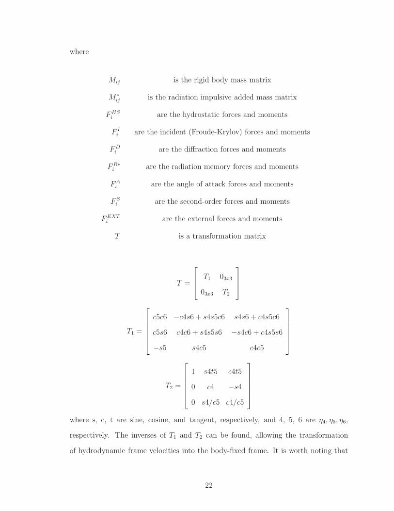
where
Mij is the rigid body mass matrix
M∗ij is the radiation impulsive added mass matrix
FHSi are the hydrostatic forces and moments
F Ii are the incident (Froude-Krylov) forces and moments
FDi are the diffraction forces and moments
FR∗i are the radiation memory forces and moments
FAi are the angle of attack forces and moments
F Si are the second-order forces and moments
FEXTi are the external forces and moments
T is a transformation matrix
T =
T1 03x3
03x3 T2
T1 =
c5c6 −c4s6 + s4s5c6 s4s6 + c4s5c6
c5s6 c4c6 + s4s5s6 −s4c6 + c4s5s6
−s5 s4c5 c4c5
T2 =
1 s4t5 c4t5
0 c4 −s4
0 s4/c5 c4/c5
where s, c, t are sine, cosine, and tangent, respectively, and 4, 5, 6 are η4, η5, η6,
respectively. The inverses of T1 and T2 can be found, allowing the transformation
of hydrodynamic frame velocities into the body-fixed frame. It is worth noting that
22

T−11 = T T
1 , but T−12 6= T T
2 since the Euler angle rates are not orthogonal.
The radiation terms, M∗ij and FR∗
i , arise from the fact that the acceleration po-
tential is used to move the body acceleration dependent component of the force to
the other side of the rigid body equations of motion. The derivation of this term is
described in the next section.
2.9 The Acceleration Potential
The “acceleration potential”, given by ψ, is defined as ψ = ∂φ∂t
. Its use in this
formulation is driven by two motivations. First, it allows the direct solution of the
∂φ∂t
term in the pressure equation (2.33). This is very beneficial when using the
body-exact approach, as the time-derivative of the potential is solved for at each
time-step. This avoids numerical difficulties with repanelization techniques and using
finite differencing schemes. Some examples of this are given later.
The second motivation of this method is that the acceleration potential can be
written in terms of the body acceleration, vi. Since this is an unknown, special care
may be taken to move this term to the other side of the rigid body equations of
motion. Similar work has been done by Vinje and Brevig (1981) and Kang and Gong
(1990), including applications of prescribed motions. Beck et al. (1994) present a
similar method, including an iterative method to solve for the body acceleration.
Tanizawa (1995) and van Daalen (1993) discuss the special case of the acceleration
potential and how it couples to the rigid body equations of motion.
The objective is to set up a boundary value problem for the acceleration potential,
as was done for the velocity potential, since the acceleration potential also satisfies
the Laplace equation. The appropriate boundary conditions must be determined.
The deep water and far field conditions are the same as described for the velocity
potential. The free surface condition requires a knowledge of ∂φ∂t
on z = 0. This
is known from the linearized free surface conditions, Eqns. (2.45) and (2.46). The
23

corresponding body boundary conditions are more difficult to derive, as they involve
time-derivatives in the hydrodynamic and body frames.
The body boundary conditions given in Eqns. (2.40) through (2.42) are used, and
the appropriate time-derivatives are taken. Two identities are used in this derivation.
δ
δt=
∂
∂t+ V · ∇ (2.57)
(∂
∂t)hydrodnymic = (
∂
∂t)body + ω× (2.58)
where V is the body node velocity, given by V = v + ω × r, and δδt
is the time-
derivative, in the body frame, following the body node. The second equation relates
time-derivatives between two frames.
The diffraction body boundary condition is found by partial differentiation with
respect to time, in the hydrodynamic frame, of Eqn. (2.40)
∂
∂t(N·∇φD) =
∂
∂t(−N·∇φI) (2.59)
the chain rule is applied, and Eqn. (2.58) is applied to the unit normals. Realizing
that (∂N
∂t)body = 0, the resulting equation is
N·∇ψD = −N·∇ψI − (ω × N) · (∇φD + ∇φI) on CH (2.60)
The radiation body boundary condition is found by taking the time-derivative of
Eqn. (2.41) in the body frame, following the node.
δ
δt(N·∇φR) =
δ
δt(V · N) =
δ
δt[v ·N + ω · (r × N)] (2.61)
24

and since ( δNδt
)body = 0, the left and right-hand sides can be rewritten
(δ
δt)body(v · N + ω · (r × N)) = v · N + ω · (r × N) (2.62)
(δ
δt)body(N·∇φR) = N · [( ∂
∂t)body(∇φR) + (V · ∇)∇φR] (2.63)
where (∂
∂t)body(∇φR) = (
∂
∂t)hydrodynamic(∇φR) − ω×(∇φR) (2.64)
resulting in
N·∇ψR = v · N + ω · (r ×N) − (ω ×N) · ∇φR −N · (V · ∇)∇φR on CH (2.65)
The angle of attack body boundary condition is derived similarly to the radiation
condition, by taking the body frame time-derivative of Eqn. (2.42).
δ
δt(N·∇φA) =
δ
δt(Uo(−η6N2 + η5N3)) (2.66)
and, assuming Uo to be constant, results in
N·∇ψA = −(ω ×N) · (∇φA −Uo) on CH (2.67)
where Uo = (Uo, 0, 0) for the case of constant forward speed.
Eqns. (2.60), (2.65), and (2.67) are the equivalent diffraction, radiation, and angle
body boundary conditions for the acceleration potential. The right-hand sides of these
equations can all be determined once the φ problem is solved. The result is a mixed
boundary value problem for ψ written in the hydrodynamic frame.
At this point, the acceleration potential has been described such that the ∂φ∂t
term in the pressure equation (2.33) can be solved for directly. This next step is
to move the body acceleration terms, v and ω, to the other side of the rigid body
equations of motion. This is done by splitting the radiation acceleration potential
25

into two components, impulsive (ψR,I) and memory (ψR,M), subject to the following
boundary conditions.
ψR = ψR,I + φR,M (2.68)
N·∇ψR,I = v · N + ω · (r ×N) on CH (2.69)
N·∇ψR,M = −(ω × N) · ∇φR − N · (V · ∇)∇φR on CH (2.70)
ψR,I = 0 on CF (2.71)
ψR,M = ψR on CF (2.72)
Combining the boundary conditions, we recover the original radiation acceleration
potential problem. For simplicity of notation, let χ ≡ ψR,I . This impulsive problem,
which is only a function of the body accelerations, is further reduced into six canonical
problems.
χ =
6∑
i=1
viχi (2.73)
where vi and χi are the acceleration and the scaled acceleration potential, due to a
unit body acceleration, in the ith mode of motion. They must satisfy the following
boundary conditions
N · ∇χi = Ni for i = 1..6 on CH (2.74)
χi = 0 for i = 1..6 on CF (2.75)
The solution of this boundary value problem is where the M∗ij and FR∗
i terms
originate. The ψR,M solution goes into the pressure equation and is then integrated
around the entire body, resulting in an expression for FR∗i that excludes the body
acceleration component. The solution of χi everywhere on the body can be used to
find the radiation impulsive added mass matrix, M∗ij , and the components are given
26
by
M∗ij = ρ
∫
L
dx
∫
CH
χjNi dl (2.76)
Breaking down the radiation acceleration potential in such a way allows moving
the unknown body acceleration terms to the other side of the equations of motion,
as given in Eqn. 2.55. This reduces numerical instabilities and increases accuracy in
the coupled hydrodynamic and rigid body equations.
2.10 Viscous Forces
The effects of viscosity are not captured in potential flow theory. Usually these
effects are small enough that ignoring viscosity is justified. However, there are in-
stances where they must be included, such as additional viscous roll damping. The
model used in this formulation is that of Himeno (1981), where emprical corrections
are added for viscosity. The amount of additional damping is dependent on the hull
form or section shape, and is usually determined from experimental results.
Besides viscous roll damping, other motions must be considered. Surge, sway, and
yaw have no restoring mechanisms. Adding viscous damping terms in those degrees of
freedom is important, especially in the case of free motions, where the vessel may drift
off. Especially important is the case of zero encounter frequency, where potential flow
predicts zero damping. The maneuvering equations and coefficients suggest otherwise,
because they include viscous effects. The goal is to include these effects in a viscous
forcing model, while not “double counting” the potential flow results.
An approach to solve this problem is discussed by Bailey et al. (1998). They
include an additional damping component, due to viscosity, based on the assumption
that B22 = −Yv and B66 = −Nr at the zero frequency limit. B22 and B66 are the
sway-sway and yaw-yaw damping coefficients in seakeeping theory, respectively. Yv
and Nr are the sway-sway and yaw-yaw stability derivatives in maneuvering theory,
27
respectively. Bailey et al. (1998) propose a linear ramp function, up to some limiting
frequency, where this viscous term is simply added to the potential flow results. Fossen
and Smogeli (2004) and Fossen (2005) present a similar approach, but extend it to
all six degrees of freedom by adding a viscous addition to all the diagonal terms of
the damping matrix.
The simplified method used here resembles that in Bailey et al. (1998). Addi-
tionally, we use a semi-empirical method for calculating the stability derivatives of
interest. As discussed by Clarke et al. (1983), the hull is assumed to be a low as-
pect ratio wing and the maneuvering coefficients are a function of the length to draft
ratio of the ship. A more advanced method includes regression analysis to develop
empirical formulas to correct the simplified coefficients.
Y ′v = Co(A1 +B1) (2.77)
Y ′r = Co(A2 +B2) (2.78)
N ′v = Co(A3 +B3) (2.79)
N ′r = Co(A4 +B4) (2.80)
where C0 = −π(TL)2 (2.81)
A1 = 1.0 B1 = 0.4CBB
T(2.82)
A2 = −0.5 B2 = 2.2B
L− 0.08
B
T(2.83)
A3 = 0.5 B3 = 2.4T
L(2.84)
A4 = 0.25 B4 = 0.039B
T− 0.56
B
L(2.85)
where L,B, T, CB are the length, beam, draft, and block coefficient of the hull. The
Ai coefficients come from the low aspect ratio wing theory, and the Bi coefficients
come the linear regression analysis of the velocity derivatives. The dimensional values
28

Y ′v Y ′
r N ′v N ′
r
Low AR wing (B coeff =0) -0.01025 0.00513 -0.00513 -0.00256Semi-empirical -0.01743 0.00396 -0.00653 -0.00274Experiments -0.0164 0.00291 -0.00691 -0.0032
Table 2.1: Series 60 CB=0.7 Sway and Yaw Maneuvering Coefficients
of these coefficients are given by
Yv = Y ′v0.5ρL
2U (2.86)
Yr = Y ′r0.5ρL
3U (2.87)
Nv = N ′v0.5ρL
3U (2.88)
NR = N ′r0.5ρL
4U (2.89)
where ρ is the fluid density and U is approximated to be the mean ship speed, or Uo.
The Series-60 hull (with 0.7 block coefficient) is used to check this semi-emperical
method. The comparisons between the predicted values using low aspect ratio wing
theory, the semi-emperical method (low aspect ratio plus regression), and experimen-
tal results are shown in Table 2.1.
The results indicate that the semi-emperical formulation improves the estimate
of the coefficients. These estimates do not have to be exact. The maneuvering
coefficients are added to the potential flow damping up to a certain frequency, ωv,
using a linear ramp. Fossen and Smogeli (2004) use the following
Fi,visc = −Bii,viscvi(1 − ωe
ωv
), ωe ≤ ωv (2.90)
Fi,visc = 0, ωe > ωv (2.91)
for i = 2, 6 or in sway, and yaw, and B22,visc = −Yv, B66,visc = −Nr. ωv is based
on comparing the potential flow damping coefficients with experiments, and can be
given by the non-dimensional value of 12.5, or ωv = 12.5√
gL≈ 3rad/s for the S-175,
29

for example. This gives a form of a viscous force that can be added to the rigid body
equations of motion, as presented earlier.
30
CHAPTER III
Numerical Techniques
3.1 Source Distribution Method
At each time-step a mixed boundary value problem must be solved; the potential
is given on the free surface and the normal derivative of the potential is given on
the body surface. In this formulation, the source distribution technique is used.
Desingularized sources are used to model the free surface, while constant strength
flat panels are used to model the body wetted surface. The potential at any point in
the fluid domain can be found by
φi =∑
CF
σjG(xi; ξj) +
∫
CH
σjG(xi; ξj)dl (3.1)
where φi can be the velocity or acceleration potential at some field point, xi, anywhere
in the domain. ξj is the location of a source point with corresponding source strength
σj . The first term on the right-hand side of Eqn. (3.1) is the summation of the
influence of the isolated desingularized sources on the free surface, while the second
term includes the integral over the panels on the body. G(xi; ξj) is a Rankine source
31

Green function
G(xi; ξj) = ln r (3.2)
r = |xi − ξj| (3.3)
where r is the distance between a field point and a source point
Applying the boundary conditions and using Eqn. (3.1), the integral mixed bound-
ary value equations can be discretized to form a system of linear equations, shown
in Eqns. (3.4) and (3.5). On the free surface, desingularized sources are distributed
outside of the domain such that the the source points never coincide with collocation
or node points, avoiding singularities. Isolated sources are used rather than a distri-
bution, reducing the complexity of the influence matrix. The desingularized distance
is given by the square root of the local mesh size.
∑
CF
σj ln |xi − ξj| +∫
CH
σj ln |xi − ξj |dl = φi xi ∈ CF (3.4)
∑
CF
σj
∂ ln |xi − ξj|∂N
+
∫
CH
σj
∂ ln |xi − ξj |∂N
dl =∂φi
∂Nxi ∈ CH (3.5)
32

where xi = a point on the boundary of the domain
ξj = a source point
σj = the source strength
φi = the given potential on the free surface
∂φi
∂N= the given normal derivative of the potential on the body
CF = the free surface contour
CH = the hull contour
∂∂N
= N · ∇
The body surface is modeled using panels, which are more suitable for arbitrarily
shaped bodies. The resulting discretized equations are given by
NF∑
j=1
σj ln |xi − ξj | +NB∑
j=1
σj
∫
∆lj
ln |xi − ξj|dl = φi xi ∈ CF (3.6)
−πσi +
NF∑
j=1
σj
(xi − ξj) ·Ni
|xi − ξj |2+
NB∑
j=1,j 6=i
σj
∫
∆lj
(xi − ξj) · Ni
|xi − ξj|2dl =
∂φi
∂Nxi ∈ CH (3.7)
where Ni is the unit normal on body panel i, NF is the number of free surface nodes,
and NB is the number of body nodes.
Eqns. (3.6) and (3.7) can be written in matrix form, Aijσj = bi, where Aij is
the influence matrix, determined by the left hand sides of the equations, σj are the
unknown source strengths, and bi is the right-hand side of the equations. The matrix
is inverted using Gaussian elimination and the source strengths can be determined.
Once the source strengths are known, the potential and its derivatives can be
computed anywhere in the domain. In particular, we are interested in φ and its
33

gradients on the body and free surface boundaries. Similar influence matrices can be
set up to determine these values, given the source strengths. Details can be found in
Appendix B. This approach can be used to solve the velocity potential or acceleration
potential, including each of the individual components.
The case of a deeply submerged body can be used as a preliminary validation of
the influence matrices. There is no free surface and the velocity potential can often
be given analytically, depending on the body shape. Appendix C provides a detailed
verification of the influence matrices derived in Appendix B, using a known analytic
solution for the velocity potential for the case of a deeply submerged circular section.
Some interesting results arise, suggesting that a constant strength flat panel method
cannot be used to compute the second space derivatives of the velocity potential
on the body. These values are required to set up the boundary value problem for
the radiation acceleration potential, given in Eqn. (2.65). The alternative is to
numerically estimate these values using the fluid velocity, or ∇φ, on adjacent panels
and differentiate them along the tangential direction. Details and validations are
presented in Appendix C.
3.2 Domain Discretization
There are a variety of ways to discretize the domain boundaries, depending on
the problem being addressed. In this formulation the free surface is broken up into
an inner and outer region, where the inner region resolves the waves and the outer
region is used as a numerical beach. For single frequency oscillations at ω, the inner
region can span several wavelengths on either side of the body, where the wavelength
is given by the deep water dispersion relation, λ = 2πgω2 . To resolve the radiated waves,
typically 30 nodes are distributed per wavelength in the inner region. The number
of wavelengths and nodes per wavelength can be varied. For multiple frequencies, a
discretization can be derived where the node spacing gradually increases as the points
34

are farther from the body. This can resolve short waves near the body and long waves
farther away. Convergence and validations are presented later.
The outer region acts as a numerical beach to prevent wave reflection. 20 nodes are
distributed over 80 wavelengths with exponentially increasing spacing, as determined
by Lee (1992), with the following distribution
dy2i = dy ∗ 1.0378i(i−1)
2 for i = 1..20 (3.8)
where dy is the spacing of the outermost nodes in the inner domain. This distribution
is sufficient to effectively delay wave reflection for about 15 periods of oscillation. If
a longer time simulation is desired, the coefficient and number of outer domain nodes
must be adjusted. Lee (1992) discusses this in detail for the two-dimensional problem.
The desingularized sources on the free surface are distributed outside the domain
a small distance above the calm water surface. The desingularized distance, ld, is
given by
ld =√
lcdy (3.9)
where lc is some characteristic length scale of the problem, the panel size or smallest
node spacing, for example. This problem is discussed by Cao et al. (1991).
The body is modeled using flat panels because they are more suitable for arbi-
trary body shapes. The two-dimensional method by Zhang (2007) utilizes a “rubber-
banding” scheme, where the number of panels remains the same, and the influence
matrix size is constant. This has significant benefits, including the ability to use an
iterative solver. However, for the body-exact approach, we must allow sections to
come out of the water entirely. This would result in body panel resolution that could
be orders of magnitude smaller than free surface resolution, leading to ill-conditioned
matrices, and resulting in poor numerics.
The alternate approach is to use a “fixed” panelization, in which the body is pan-
35

elized once, using a preprocessor. This produces better influence matrices and there is
never a need to curve fit the the body between time-steps, saving some computation
time. This method requires direct matrix inversion, which is the most computation-
ally expensive step in the entire formulation. However, with the problems stated in
this formulation, that is beneficial. Since each of the components of the velocity po-
tential (3 total) and acceleration potential (10 total) have the same influence matrix,
a single inverted matrix can be used multiple times to solve for each component. The
computational time to back-substitute is far less than that to iteratively solve the
matrix problem for each component.
3.3 Time-Stepping
The free surface elevation and potential are updated using the kinematic (2.45)
and dynamic (2.46) free surface boundary conditions. The rigid body equations of
motion, Eqns. (2.55) and (2.56) must also be integrated in time for the case of free
motions. Time-stepping is done using a fourth-order Adams-Bashforth scheme
P 1 = P 0 +∆t
24(55P 0
t − 59P−1t + 37P−2
t − 9P−3t ) (3.10)
where P is the function being numerically integrated, Pt is the time-derivative, and
the superscripts indicate which time-step the values are taken from, i.e. 0 is the
current time-step. The quantities that are integrated in such a manner are P = φ, ζ
for the free surface conditions and P = v, η for the body equations of motion.
The time-step size can be chosen as a number of time-steps per period. For
example, using T/100 ≤ ∆t ≤ T/200 is usually sufficient. The spatial resolution,
especially on the free surface, can introduce stability problems if the time-step is too
coarse. This is discussed by Park and Troesch (1992) and Wang and Troesch (1997),
36

including a description of a free surface stability index, FSS.
FSS = πg∆t2/∆x (3.11)
An acceptable value for the stability index is dependent on the discretization and
integration schemes used on the free surface. It is aslo dependent on the types of
boundary conditions. As a conservative estimate, a value of FSS ≤ 1 will ensure a
stable free surface throughout the computations.
3.4 Body and Free Surface Intersection
In linear theory, the free surface conditions are satisfied on the calm water surface,
z = 0, and the body boundary conditions are satisfied on the mean position of the
body. In the body-exact formulation, the body geometry changes depending on the
motions, and we want to integrate the pressure on the actual wetted surface of the
hull. This requires a knowledge of the intersection points between the body and the
free surface. Using the exact free surface would be very challenging, since only the
incident wave is well defined. As a compromise, we can model the intersection of
the body up to the incident free surface. The remaining perturbation free surface
conditions are linearized about a plane defined by the intersection of the exact body
and the incident wave. This differs from the weak-scatterer formulation of Pawlowski
(1992), which linearizes the free surface conditions about the incident wave profile.
We want to integrate up to z = ηI , and the linear incident potential in Eqn. (2.38)
is only valid up to z = 0. Using this potential and the linearized form of the pressure
equation, p = −ρ(∂φ∂t
+ gz), from Eqn. (2.33), we find that p 6= 0 on z = ηI and the
dynamic free surface condition is violated. A simple correction, widely used in the
offshore industry, is to scale the incident wave potential by modifying the ekz term
37

with ek(z−ηI ) when evaluating the pressure, resulting in
φI =iga
ωoe−ik(xocosβ+yosinβ)eiwotek(z−ηI ) (3.12)
This formulation is similar to that of Wheeler (1970), but assumes deep water. We
can verify the dynamic free surface condition using this form of the incident potential.
For example, linear waves traveling in the xo-direction (β = 0) are given by
φI =iga
ωo
ei(wot−kxo)ek(z−ηI ) (3.13)
ηI = aei(wot−kxo) (3.14)
We can evaluate the linear incident pressure by examining
p∗ =p
ρg= aei(wot−kxo)ek(z−ηI ) − z (3.15)
and verify that p∗ = 0 on the incident wave elevation. It is evident that solving for the
pressure on z = ηI results in zero pressure, thus satisfying the dynamic free surface
condition. This modification to the incident potential is sufficient to allow integration
up to the incident wave using the body-exact approach.
3.5 Section Exit and Entry
One of the main reasons for using the body-exact approach is the ability to get
accurate solutions for large amplitude motions. This includes allowing sections to
come out of and go back into the water. This is done simply by stopping calculations
as a section comes out of the water, then re-initializing φ and φt to zero at that
section. As the section enters the water, the two-dimensional problem is solved as
usual. This often leads to spikes in the pressure, as you would expect from an impact
problem.
38

3.6 Radial Basis Functions
The ∂φ∂x
term in the pressure equation (2.33) can be approximated by using radial
basis functions (RBF). Using this method to numerically solve partial differential
equations is discussed by Kansa (1999). A more general discussion of RBFs is pre-
sented by Buhmann (2000).
Once the two-dimensional problem is solved for each section, the velocity poten-
tials at nodes on the entire body are given as a function of the Euclidean distance
between the nodes.
fj(xi) ≡ f(|xi − xj |) (3.16)
φ(xi) =
N∑
j=1
αjfj(xi) + αN+1 (3.17)
N∑
j=1
αj = 0 (3.18)
where f is one of many possible basis functions. The final equation (3.18) for the
coefficients αj is to ensure uniqueness. These expansion coefficients are found by
setting up a system of N + 1 equations, such that
P =
1
...
1
∈ RN
F =
f1(x1) . . . fN (x1)
... fj(xi)...
f1(xN ) . . . fN (xN)
∈ RNxN
H =
F P
P T 0
∈ R(N+1)x(N+1)
39
and the N + 1 system can be rewritten in matrix form
Hijαj = φi (3.19)
with φN+1 = 0. The interpolation expansion coefficients can be found after matrix
inversion
αj = [Hij]−1φi (3.20)
These coefficients can be used to interpolate the data in three-dimensional space
and to find derivatives at any point. The x-velocity of the fluid is found by taking
the partial derivative of the basis function with respect to the x-direction.
∂φ(xi)
∂x=
N∑
j=1
αj∂fj(xi)
∂x(3.21)
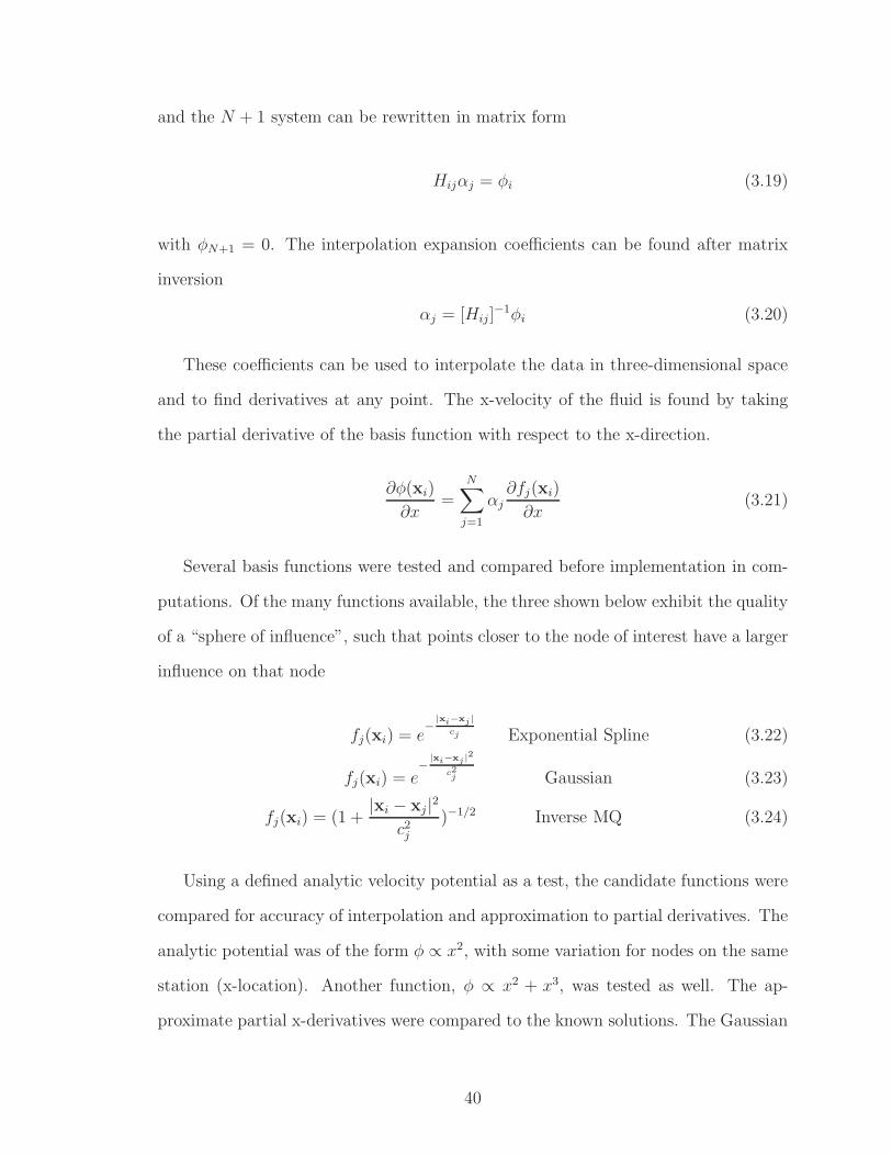
Several basis functions were tested and compared before implementation in com-
putations. Of the many functions available, the three shown below exhibit the quality
of a “sphere of influence”, such that points closer to the node of interest have a larger
influence on that node
fj(xi) = e−
|xi−xj |
cj Exponential Spline (3.22)
fj(xi) = e−
|xi−xj |2
c2j Gaussian (3.23)
fj(xi) = (1 +|xi − xj |2
c2j)−1/2 Inverse MQ (3.24)
Using a defined analytic velocity potential as a test, the candidate functions were
compared for accuracy of interpolation and approximation to partial derivatives. The
analytic potential was of the form φ ∝ x2, with some variation for nodes on the same
station (x-location). Another function, φ ∝ x2 + x3, was tested as well. The ap-
proximate partial x-derivatives were compared to the known solutions. The Gaussian
40

0 0.2 0.4 0.6 0.8 10
1
2
3
4
5
6
7
8
9
10
cj as a fraction of the ship length, L
% m
ean
erro
r and
sta
ndar
d de
viat
ion
RBF sphere of influence: accuracy comparison with ψ = x2
Gaussian errorGaussian stddevInv. MQ errorInv. MQ stddev
Figure 3.1: RBF cj comparison, φ ∝ x2
0 0.2 0.4 0.6 0.8 10
1
2
3
4
5
6
7
8
9
10
cj as a fraction of the ship length, L
% m
ean
erro
r and
sta
ndar
d de
viat
ion
RBF sphere of influence: accuracy comparison with ψ = x2 + x3
Gaussian errorGaussian stddevInv. MQ errorInv. MQ stddev
Figure 3.2: RBF cj comparison, φ ∝ x2 + x3
41

(3.23) and Inverse Multi-Quadratic (3.24) functions proved to be the more accurate
basis functions. Their accuracy depends on the “sphere of influence” term, cj. Sev-
eral tests cases were run to determine an the optimum value of this variable. The
test cases involved computing the partial x-derivative of the RBF approximation and
comparing it to the known solution. Both the Gaussian and Inverse Multi-Quadratic
functions were evaluated. Mean error and standard deviation were considered as
benchmarks of comparison. The percentages (based on the mean absolute value of
the exact solutions) of mean error and standard deviation are shown as functions of
cj in Figures 3.1 and 3.2. They indicate that using approximately L/4 yields good
results for both functions. The estimation at the end sections is not as good because
the interpolation is only one-sided.
Implementing this basis function in the computations resulted in occasional in-
stabilities, especially for extreme amplitude motions at higher frequency. The source
of the instability is the ∂φ∂x
term estimated by the RBF. It is a result of very high
condition numbers in the matrix inversion routines, which use Gaussian elimination.
Several attempts were made to correct this, but some instabilities remained. The
Exponential Spline function, Eqn. (3.22), although less accurate, had much better
condition numbers. The final selection for use in the code was an exponential function
of power 1.5, as shown in Eqn. (3.25). This function was much more accurate than
the Exponential Spline while being better conditioned for matrix inversion than the
Gaussian function.
fj(xi) = e−
|xi−xj |1.5
c1.5j (3.25)
The results were again verified against analytic velocity potentials. This RBF
gives accurate approximations to ∂φ∂x
, while remaining stable when implemented in
the real code for actual ship hulls.
42

3.7 Computation Time
An important aspect of this work is computational efficiency. The code can achieve
real-time simulations on a high-end desktop computer with multiple cores, which are
common today. The implementation of a strip theory allows very efficient use of multi-
core machines. The most computationally expensive portion is matrix inversion,
followed by back-substitution of the many right-hand sides, that must be done at
each time-step. Most of these matrix operations can be done independently for each
station. The matrix inversion and back-substitution routines used are available in
LINPACK, written in Fortran. They are efficient, accurate, and well-suited for this
type of problem.
For example, consider a ship with 20 stations, where each station has 100 free
surface nodes on either side of the body (including the beach) and 50 panels to
model the body. This requires inverting 20 influence matrices with size 250x250
at each time-step. In this example, it takes approximately 0.02sec/station/time-
step of wall-clock time using an Intel R©CoreTM2 2.4GHz processor and Intel R©Fortran
compiler, without parallelization. Solving the forward speed problem with radial basis
functions introduces more matrix inversions, and an additional 0.4sec/time-step. All
computations take 0.8sec/time-step in this example. If the period of oscillation is
about T = 15sec and the time-step size is about T/100 (typical values for real ship
simulations), the simulation will execute five times slower than real-time. However,
if the compiler supports multi-core directives, significant improvements can be made.
The two-dimensional problems are independent of one another, and can be solved in
parallel.
The OpenMP architecture supported in the Intel R©Fortran compiler is ideal for
these sort of computations. The execution speed scales very well with the number of
processors or cores, up to the number of stations. The current code has been tested
for parallelization performance on two-, four-, and eight- core machines, common for
43

present-day desktops. There is some overhead that will not scale with the number
of cores, unless the code is optimized in more detail. Regardless, exploiting the
independence of the two-dimensional problems offers significant speed gains. For
example, running the same test case with parallelization on an eight-core machine
shows 85 − 90% average CPU utilization, resulting in simulations faster than real-
time.
44

CHAPTER IV
Two-Dimensional Results
The origin of this section is based on the two-dimensional boundary element
method developed by Zhang (2007). One fundamental departure from that work
is the direct solution the acceleration potential, instead of numerical differentiation
of the velocity potential, which is a significant improvement. It offers better solutions
of ∂φ∂t
and can be coupled with the equations of motions, as described earlier. Many
other aspects, such as panelization models, spatial and temporal discretization, and
numerical techniques, have been developed to better suit the body-exact approach.
These factors complicate a direct comparison of the current and original methods.
The following sections go through a range of test cases to verify the two-dimensional
computations. In many cases, select results are shown using the approach originally
given by Zhang (2007).
4.1 Validation of the Acceleration Potential
The form of the acceleration potential derived in this approach can be compared
with other methods. Two methods are chosen in this case. The first is the original
numerical differentiation of ∂φ∂t
using central or backwards differencing schemes, as
originally done in Zhang (2007). The second is the method discussed by Kang and
Gong (1990), in which a boundary value problem is set up to solve for δφδt
, as defined
45

-5e+07
-4e+07
-3e+07
-2e+07
-1e+07
0
1e+07
2e+07
3e+07
4e+07
5e+07
6e+07
0 5 10 15 20 25
sect
iona
l for
ce [k
N/m
]
time [s]
Sectional Heave Force on Circular Cylinder
rad-numdiffrad-delta t
rad-partial tv2-numdiffv2-delta t
v2-partial t
Figure 4.1: Circular Cylinder Forced Heave, a = 2m, R = 10m, ω2R/g = 1.5
in Eqn. (2.57).
The sectional heave force on a two-dimensional circular cylinder is calculated at a
range of amplitudes. The non-dimensional frequency is ω2R/g = 1.5 where R = 10m.
The amplitudes of motion are at a = 2, 4, 6m. Figures 4.1 through 4.3 show the
radiation, “rad”, and second order, “v2”, components of the force on the section in
each of these cases. These components correspond to the first and second order terms
found in the pressure equation (2.33). The three methods are labeled “numdiff”,
“delta”, and “partial” for the numerical differentiation, δφδt
, and ∂φ∂t
formulations,
respectively. The hydrostatic force is not shown, since it would be identical between
the methods.
In Figure 4.1, all three sets of results agree well. There are some spikes in the
radiation force from numerical differentiation. They are due the fact that the dif-
ferencing scheme has difficulties if the number of panels changes between time-steps.
As the amplitude increases, significant nonlinearities start to arise in the radiation
46

-1e+08
-5e+07
0
5e+07
1e+08
1.5e+08
0 5 10 15 20 25
sect
iona
l for
ce [k
N/m
]
time [s]
Sectional Heave Force on Circular Cylinder
rad-numdiffrad-delta t
rad-partial tv2-numdiffv2-delta t
v2-partial t
Figure 4.2: Circular Cylinder Forced Heave, a = 4m, R = 10m, ω2R/g = 1.5
-2e+08
-1.5e+08
-1e+08
-5e+07
0
5e+07
1e+08
1.5e+08
2e+08
0 5 10 15 20 25
sect
iona
l for
ce [k
N/m
]
time [s]
Sectional Heave Force on Circular Cylinder
rad-numdiffrad-delta t
rad-partial tv2-numdiffv2-delta t
v2-partial t
Figure 4.3: Circular Cylinder Forced Heave, a = 6m, R = 10m, ω2R/g = 1.5
47

component, and these spikes get more severe. In the body-exact formulation, some
of the advantages of a direct solution for ∂φ∂t
can be seen in these results, especially in
Figures 4.2 and 4.2
The method proposed by Kang and Gong (1990) offers the same advantages and
compares very well with the current method. However, the problem becomes diffi-
cult when considering how the free surface conditions must be specified. The entire
boundary value problem is written in terms of body-frame time-derivatives, including
the free surface. For example, in six degree-of-freedom motions, the body rotation
rates become part of the free surface conditions. Numerical accuracy becomes a con-
cern, as there would be sums and differences of large numbers, coming from ω × r
contribution to the free surface conditions. Therefore, the approach derived earlier,
to set up a boundary value problem for ψ (or ∂φ∂t
) is a better alternative.
4.2 Convergence Studies
The convergence characteristics of the numerical methods used must be examined.
This gives an idea about what sort of parameter ranges are acceptable for compu-
tational simulations. The studies here are for a two-dimensional circular section of
radius R = 10m, with a forced heave motion amplitude of 1m. The mean position
coincides with half of the cylinder being submerged. Two oscillation frequencies are
used, ω(R/g)0.5 = 0.6, 1.6, in order to observe convergence a case of long and short
wavelengths generated on the free surface. Using R = 10m is convenient in that the
non-dimensional frequency is approximately equal to the dimensional value. After
the time simulation, the resulting heave force time series are Fourier transformed.
Corresponding to linear seakeeping theory, the first-order component of the hydro-
dynamic force is divided into added mass and damping coefficients; the components
that are in phase with the acceleration and velocity of the body, respectively.
Four parameters are studied: time-step size, body panel resolution, inner free
48

surface resolution, and free surface domain size. The time-step size is based on the a
fraction of the period of oscillation. Body panel resolution is based on the number of
panels used to model the circular section. Inner free surface resolution is the number
of nodes on the free surface near the body with spacing comparable to the body panel
spacing. Free surface domain size is the length the free surface extends to, excluding
the numerical beach.
Each parameter is analyzed by changing its value while leaving the others fixed.
The benchmark is a high resolution set of parameters where a converged solution
exists. This can be determined by trial and error, using multiple iterations. The con-
vergence of each parameter can be checked by decreasing that parameter’s resolution.
The convergence of the coefficients is presented in Figures 4.4 and 4.5. The coeffi-
cients are non-dimensionalized using ρ, g, R, and A, the fluid density, gravitational
acceleration, cylinder radius, and submerged area, respectively.
The four parameters are plotted together against the fraction of the high resolu-
tion, or benchmark, values. The benchmark values used are a time-step of T/400,
250 total body panels (half are submerged in the body’s mean position), 40 inner free
surface nodes, and free surface length of 1000m or 100R. The body panel number
shows the same type of convergence in the Figures, and is important to get accu-
rate solutions. The time-step and inner free surface resolution converge much faster,
and appear to be almost constant. The time-step converges so quickly because of
the acceleration potential formulation and higher order schemes used to evolve the
free surface conditions. The free surface extent converges more slowly in the low
frequency case, shown in Figure 4.4, because the radiated wavelength is significantly
longer. The long and short wavelengths are approximately 172m and 24m. This
suggests that the numerical techniques described can be used to model a range of
wavelengths accurately.
49

0.725
0.73
0.735
0.74
0.745
0.75
0.755
0.1 0.2 0.3 0.4 0.5 0.6 0.7 0.8 0.9 1
Add
ed M
ass,
a33
/(ρA
)
Fraction of High Resolution Value
Convergence: Circular Cylinder Added Mass at ω(R/g)0.5=0.6
time-steppanel size
FS resFS extent
0.61
0.611
0.612
0.613
0.614
0.615
0.616
0.617
0.618
0.619
0.62
0.621
0.1 0.2 0.3 0.4 0.5 0.6 0.7 0.8 0.9 1
Dam
ping
, b33
/(ρA
) (R
/g)0.
5
Fraction of High Resolution Value
Convergence: Circular Cylinder Damping at ω(R/g)0.5=0.6
time-steppanel size
FS res.FS extent
Figure 4.4: Convergence of Circular Cylinder in Heave, ω = 0.6
50

0.785
0.79
0.795
0.8
0.805
0.81
0.815
0.82
0.1 0.2 0.3 0.4 0.5 0.6 0.7 0.8 0.9 1
Add
ed M
ass,
a33
/(ρA
)
Fraction of High Resolution Value
Convergence: Circular Cylinder Added Mass at ω(R/g)0.5=1.6
time-steppanel size
FS resFS extent
0.1
0.102
0.104
0.106
0.108
0.11
0.112
0.114
0.1 0.2 0.3 0.4 0.5 0.6 0.7 0.8 0.9 1
Dam
ping
, b33
/(ρA
) (R
/g)0.
5
Fraction of High Resolution Value
Convergence: Circular Cylinder Damping at ω(R/g)0.5=1.6
time-steppanel size
FS res.FS extent
Figure 4.5: Convergence of Circular Cylinder in Heave, ω = 1.6
51

4.3 Small Amplitude Radiation
The numerical results must be validated against experiments. Vugts (1968) offers
a range of experimental data on various two-dimensional cross-sections. The sections
compared are the circular cylinder and box barge types. The circular section has a
radius R = 10m, and the box barge used has beam B = 20m and draft T = 10m.
In either case, the non-dimensional frequency is given as ω(B/2g)0.5, consistent with
the conventions used by Vugts (1968).
The circular cylinder hydrodynamic coefficients are compared using the current
method, an alternate free surface spacing, and the experimental results, as shown in
Figures 4.6 and 4.7. The “current method” uses the incrementally increasing node
spacing technique for the inner free surface and is independent of the frequency of
oscillation. The initial node spacing is comparable to the body panel size while the
outermost is comparable to the radius, and 80 nodes are distributed with increasing
spacing. This is the same scheme used in the convergence studies. The “Alt. FS
Grid” solutions use a constant node spacing, λ/40 in this case, to model the free
surface over two wavelengths. Both methods use the same numerical beach. The
two methods use the same number of points to model the boundaries and require the
same amount of computational effort.
The results shown agree very well with the experimental data. Moreover, they
justify the use of the free surface node distribution. The current method shows better
agreement than the computationally comparable alternate free surface grid, when
using the same number of nodes. This is especially evident at lower frequencies. The
alternate method could use a higher resolution to resolve longer waves, but this would
require more computation time.
The same set of computations can be carried out for the box barge section. The
roll problem is also examined, including the coupling between roll and sway motions.
The same sets of results are shown, in addition to “Viscous” simulations, which add
52

0.4
0.6
0.8
1
1.2
1.4
1.6
1.8
0 0.5 1 1.5 2
a 33/
(ρA
)
ω (B/2g)0.5
2D Circular Cylinder: Heave Added Mass
Current MethodAlt. FS GridVugts Exp.
0
0.1
0.2
0.3
0.4
0.5
0.6
0.7
0 0.5 1 1.5 2
b 33/
(ρA
) (B
/2g)
0.5
ω (B/2g)0.5
2D Circular Cylinder: Heave Damping
Current MethodAlt. FS GridVugts Exp.
Figure 4.6: Circular Cylinder Heave Added Mass and Damping
53

0
0.2
0.4
0.6
0.8
1
1.2
1.4
0 0.5 1 1.5 2
a 22/
(ρA
)
ω (B/2g)0.5
2D Circular Cylinder: Sway Added Mass
Current MethodAlt. FS GridVugts Exp.
0
0.1
0.2
0.3
0.4
0.5
0.6
0.7
0.8
0 0.5 1 1.5 2
b 22/
(ρA
) (B
/2g)
0.5
ω (B/2g)0.5
2D Circular Cylinder: Sway Damping
Current MethodAlt. FS GridVugts Exp.
Figure 4.7: Circular Cylinder Sway Added Mass and Damping
54

the viscous roll correction described earlier and only affect the roll moment due to
roll. The heave, sway, roll, roll due to sway, and sway due to roll result comparisons
are shown in Figures 4.8 through 4.12.
The characteristics between the current method and alternate free surface grid
technique are similar to those for the circular cylinder. The addition of the viscous
roll correction term only affects the roll due to roll damping coefficient in Figure 4.10,
as expected, improving the agreement with experiments. The roll due to roll added
mass differs from the experimental value, showing similar trends to linear theory
results. The coupling coefficients show good agreement, with the exception of the roll
due to sway damping shown in Figure 4.11. The computational results maintain the
symmetry of the coupling coefficients, a24 = a42, b24 = b42. The experiments differ,
mainly due to the effects of viscosity, especially in the damping coefficients.
Overall, the agreement with experimental results for the two-dimensional prob-
lems studied is very satisfactory. The method of gridding the free surface, as described
earlier, has also been justified. The same numerical discretization of the boundaries
is used in all the simulations. It accurately predicts the forces for a variety of oscil-
lation frequencies in all modes of motion, emphasizing the robust capabilities of the
numerical methods.
4.4 Large Amplitude Oscillations of a Circular Cylinder
The body-exact method can be validated by using test cases in which the wetted
geometry of a section changes significantly. This is especially important in sections
whose sides are not vertical, or “wall-sided”. The forced heave oscillation of a cir-
cular cylinder is a classic example of this. Yamashita (1977) presented a range of
experimental and theoretical results for this type of problem. Kent (2005) devel-
oped a numerical method using a third-order pseudo-spectral method. Zhang (2007)
also presents numerical results for this problem, using the body-exact time-domain
55

0
0.5
1
1.5
2
0 0.5 1 1.5 2
a 33/
(ρA
)
ω (B/2g)0.5
2D Box Barge (B/T=2): Heave Added Mass
Current MethodAlt. FS GridVugts Exp.
0
0.1
0.2
0.3
0.4
0.5
0 0.5 1 1.5 2
b 33/
(ρA
) (B
/2g)
0.5
ω (B/2g)0.5
2D Box Barge (B/T=2): Heave Damping
Current MethodAlt. FS GridVugts Exp.
Figure 4.8: Box Barge Heave Added Mass and Damping
56

0
0.5
1
1.5
2
0 0.5 1 1.5 2
a 22/
(ρA
)
ω (B/2g)0.5
2D Box Barge (B/T=2): Sway Added Mass
Current MethodAlt. FS GridVugts Exp.
0
0.2
0.4
0.6
0.8
1
1.2
1.4
0 0.5 1 1.5 2
b 22/
(ρA
) (B
/2g)
0.5
ω (B/2g)0.5
2D Box Barge (B/T=2): Sway Damping
Current MethodAlt. FS GridVugts Exp.
Figure 4.9: Box Barge Sway Added Mass and Damping
57
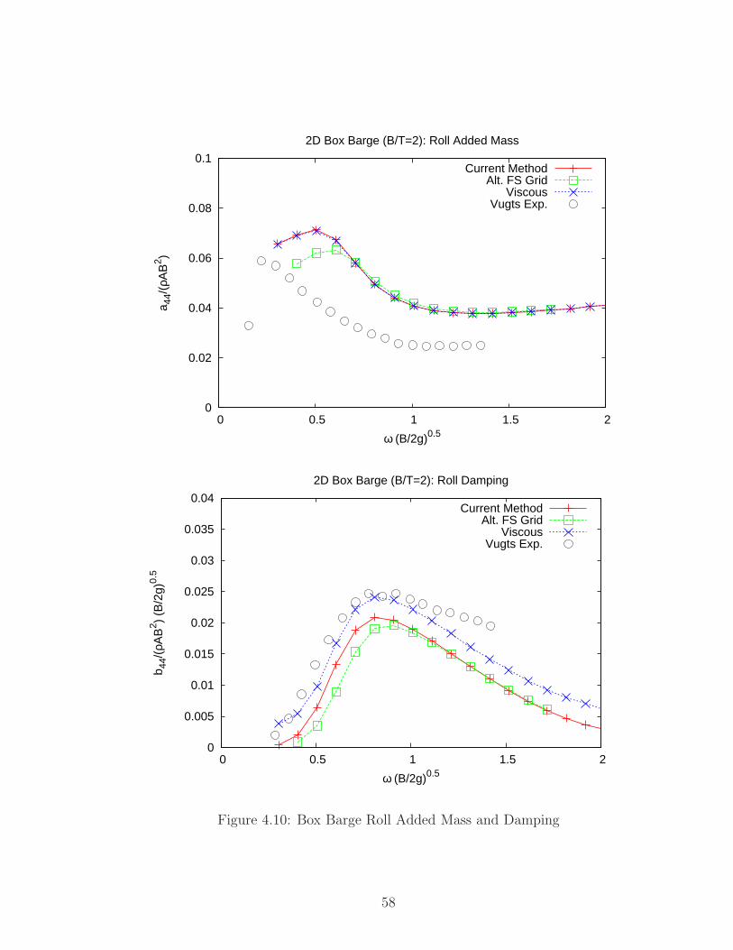
0
0.02
0.04
0.06
0.08
0.1
0 0.5 1 1.5 2
a 44/
(ρA
B2 )
ω (B/2g)0.5
2D Box Barge (B/T=2): Roll Added Mass
Current MethodAlt. FS Grid
ViscousVugts Exp.
0
0.005
0.01
0.015
0.02
0.025
0.03
0.035
0.04
0 0.5 1 1.5 2
b 44/
(ρA
B2 )
(B/2
g)0.
5
ω (B/2g)0.5
2D Box Barge (B/T=2): Roll Damping
Current MethodAlt. FS Grid
ViscousVugts Exp.
Figure 4.10: Box Barge Roll Added Mass and Damping
58

0
0.05
0.1
0.15
0.2
0.25
0.3
0 0.5 1 1.5 2
a 42/
(ρA
B)
ω (B/2g)0.5
2D Box Barge (B/T=2): Roll-Sway Added Mass
Current MethodAlt. FS GridVugts Exp.
0
0.02
0.04
0.06
0.08
0.1
0.12
0.14
0.16
0.18
0.2
0 0.5 1 1.5 2
b 42/
(ρA
B)
(B/2
g)0.
5
ω (B/2g)0.5
2D Box Barge (B/T=2): Roll-Sway Damping
Current MethodAlt. FS GridVugts Exp.
Figure 4.11: Box Barge Roll-Sway Added Mass and Damping
59
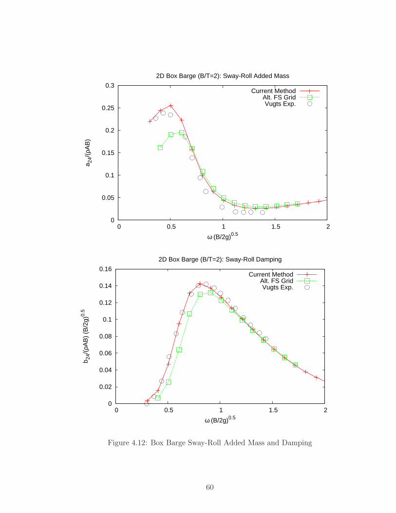
0
0.05
0.1
0.15
0.2
0.25
0.3
0 0.5 1 1.5 2
a 24/
(ρA
B)
ω (B/2g)0.5
2D Box Barge (B/T=2): Sway-Roll Added Mass
Current MethodAlt. FS GridVugts Exp.
0
0.02
0.04
0.06
0.08
0.1
0.12
0.14
0.16
0 0.5 1 1.5 2
b 24/
(ρA
B)
(B/2
g)0.
5
ω (B/2g)0.5
2D Box Barge (B/T=2): Sway-Roll Damping
Current MethodAlt. FS GridVugts Exp.
Figure 4.12: Box Barge Sway-Roll Added Mass and Damping
60

a/R=0.2 ω2R/g a33 b33 F 20 F 1
A F 2A
Yamashita (1977) 0.5 0.66 0.504 -0.01 / 0.15Kent (2005) 0.5 0.600 0.557 -0.010 0.821 0.194Zhang (2007) 0.5 0.630 0.574 -0.013 0.815 0.163Current Method 0.5 0.649 0.573 -0.014 0.808 0.202Yamashita (1977) 1.0 0.60 0.386 -0.08 / 0.45Kent (2005) 1.0 0.580 0.371 -0.086 0.615 0.491Zhang (2007) 1.0 0.600 0.406 -0.086 0.632 0.428Current Method 1.0 0.611 0.398 -0.095 0.607 0.409Yamashita (1977) 1.5 0.69 0.267 -0.15 / 0.8Kent (2005) 1.5 0.620 0.254 -0.160 0.360 0.796Zhang (2007) 1.5 0.670 0.279 -0.190 0.378 0.620Current Method 1.5 0.671 0.262 -0.193 0.327 0.590
Table 4.1: Heave Force Coefficients on Circular Cylinder, amplitude = 0.2R
approach. Their results, along with the current method, are presented as force coef-
ficients in Table 4.1.
The results are given for three non-dimensional frequencies, ω2R/g, where ω is the
circular frequency of oscillation, R is the radius, and g is the gravitational constant.
Coefficients are given for: the non-dimensional sectional added mass and damping,
a33 and b33; the second-order mean force, F 20 ; the first-order harmonic force, F 1
A; and
the second order harmonic force, F 2A. The coefficients are defined in Eqns. 4.1 through
4.5, consistent with Yamashita (1977).
a33 =Re[f(ω)]
ω2a(4.1)
b33 =Im[f(ω)]
ωa(4.2)
F 20 =
|f(0)| − ρgA
2ρga2(4.3)
F 1A =
|f(ω)|2ρgRa
(4.4)
F 2A =
|f(2ω)|2ρga2
(4.5)
where f is the sectional force time-series, Re and Im represent its real and imagi-
61

nary Fourier components, |f(ω)| indicates the amplitude of the Fourier component at
frequency ω, ρ is the water density, a is the amplitude of motion, A is the submerged
sectional area. It is worth noting that the added mass and damping are defined in
the classical sense, meaning only the first-order radiation force, while the force coeffi-
cients include the entire sectional force. The difference between the two, in this case,
is the body-exacty hydrostatic force. We do not expect the magnitude of a33 and b33
to equal F 1A, especially for increasing amplitudes of motion.
62

CHAPTER V
Strip Theory Results
The two-dimensional body-exact techniques described earlier can be extended to
three-dimensions using the strip theory approximation. In the following sections, a
variety of hull forms will be used for validations and discussion of results using the
body-exact strip theory approach. The main particulars of these vessels are listed
in Table 5.1, where L,B, T are the length, beam, and draft (all in meters). CB and
CWP are the block and waterplane coefficients of the hull, defined by
CB =V ol
LBT(5.1)
CWP =AWP
BT(5.2)
where V ol and AWP are the submerged volume and waterplane area, respectively,
when the hull is in its mean position.
L B T CB CWP
[m] [m] [m] (nd) (nd)Wigley I 3.00 0.300 0.1875 0.557 0.689Wigley III 3.00 0.300 0.1875 0.459 0.689Series 60 (0.7) 121.9 17.42 6.97 0.700 0.793m5514 (Destroyer) 142.0 19.10 6.50 0.518 0.790m5613 (Tumblehome) 154.0 18.80 5.50 0.536 0.790S-175 Containership 175.0 25.40 9.50 0.570 0.723
Table 5.1: Hull Particulars
63

The validations included are separated into radiation and wave excitation prob-
lems. The radiation problem includes isolated forced motions in one degree of free-
dom with no incident wave field, while the wave excitation problem fixes the ship and
exposes it to an incident wave field. This allows the isolation of the boundary condi-
tions, validating each separately. In both cases, the forces and moments acting on the
hull are calculated into a time-history. The amplitudes are kept small so that time-
histories may be Fourier transformed into linear components, either classical added
mass and damping terms (in phase with the acceleration and velocity, respectively)
or an amplitude and phase (typically done for exciting forces).
5.1 Small Amplitude Radiation
The body-exact strip theory approach must first be validated for small amplitude
motions. The hydrodynamic coefficients from forced motions can be compared to lin-
ear theory or experimental results. The “Wigley” hull forms have extensive numerical
and experimental results available, and will be used as test hulls. The Wigley I and
III models will be used in forced heave and pitch simulations with forward speed of
Fn = 0.3, where
Fn =Uo√gL
(5.3)
The hydrodynamic coefficients, added mass and damping, are calculated for heave
and pitch motions of the Wigley I hull and compared to other computational and
experimental results. The current method results are given, as well as a five degree-
of-freedom strip theory developed at MIT (as referenced by Nakos and Sclavounos
(1990)) based on the work of Salvesen et al. (1970), the three-dimensional code
SWAN described by Nakos (1990), and experimental results from Gerritsma (1988)
and Journee (1992).
The linear strip theory results, based on the Salvesen et al. (1970) formulation,
64

might be expected to agree exactly with the current method, given that the amplitude
of motion is small. However, we briefly examine a key difference in the treatment of
the forward speed correction to the strip theory. In the linear strip theory, a variant
of Stokes’ theorem is used to replace the ∂φ∂x
term in the pressure equation (2.33).
This was originally derived by Ogilvie and Tuck (1969), and resulting expressions for
the coefficients in heave and pitch are given by
A33 = A033 (5.4)
B33 = B033 (5.5)
A35 = A035 − B0
33Uo/ω2 (5.6)
B35 = B035 + A0
33Uo (5.7)
A53 = A053 +B0
33Uo/ω2 (5.8)
B53 = B053 −A0
33Uo (5.9)
A55 = A055 + A0
33U2o /ω
2 (5.10)
B55 = B055 − A0
33U2o /ω
2 (5.11)
where the left hand sides are the forward speed coefficients, and the superscript 0 on
the right-hand sides indicate the zero speed coefficients. The formulation is based
on the assumption that the steady velocity potential is given by Uox, ignoring the
steady perturbation potential introduced by the presence of the ship. Also, everything
is based on the mean position of the hull, consistent with linear strip theory. The
first assumption has since been shown to lead to errors, in certain cases.
The diagonal coefficients in Figures 5.1 and 5.2 show good agreement between all
the results, with the exception of pitch-pitch damping. The coupling coefficients show
better agreement in pitch due to heave (Figure 5.3) than heave due to pitch (Figure
5.4). For a symmetric hull, it is common to observe symmetry in the forward speed
coupling coefficients (Aij = −Aji, Bij = −Bji for i 6= j). This is exactly the case
65

0 0.2 0.4 0.6 0.8
1 1.2 1.4 1.6
1 2 3 4 5 6
A33
/(ρV
ol)
Wigley I Heave due to Heave Added Mass and Damping, Fn=0.3
Current MethodStrip Theory
SWAN-NakosGerritsma Exp.
Journee Exp.
0
0.5
1
1.5
2
1 2 3 4 5 6
B33
/(ρV
ol(g
/L)1/
2 )
ω (L/g)1/2
Figure 5.1: Wigley I Heave Hydrodynamic Coefficients, Fn = 0.3
for linear strip theory, as can be seen in the equations above. Timman and Newman
(1962) also showed this holds for symmetric, slender hull shapes, where the error is of
the same order as the slenderness of the hull. The current method does not exhibit
this property. The differences may be due to the use of numerical estimation of the
∂φ∂x
term in the pressure equation.
The same coefficients are calculated for the Wigley III hull form and shown in
Figures 5.5 through 5.8. An alternative set of solutions is shown using the formulation
of Ogilvie and Tuck (1969), as described earlier. Other comparisons include the code
SHIPMO, a six dogree-of-freedom linear strip theory based on Salvesen et al. (1970)
developed by Beck and Troesch (1989), the three-dimensional body-exact method of
Zhang (2007), and experimental results by Journee (1992).
The diagonal coefficients, in Figures 5.5 and 5.6 show good agreement, again
with the exception of the pitch-pitch damping coefficient. The pitch-heave coupling
66

0 0.01 0.02 0.03 0.04 0.05 0.06 0.07 0.08
1 2 3 4 5 6
A55
/(L2 ρV
ol)
Wigley I Pitch due to Pitch Added Mass and Damping, Fn=0.3
Current MethodStrip Theory
SWAN-NakosGerritsma Exp.
Journee Exp.
0
0.02
0.04
0.06
0.08
0.1
1 2 3 4 5 6
B55
/(L2 ρV
ol(g
/L)1/
2 )
ω (L/g)1/2
Figure 5.2: Wigley I Pitch Hydrodynamic Coefficients, Fn = 0.3
-0.05 0
0.05 0.1
0.15 0.2
0.25 0.3
0.35
1 2 3 4 5 6
A53
/(Lρ
Vol
)
Wigley I Pitch due to Heave Added Mass and Damping, Fn=0.3
Current MethodStrip Theory
SWAN-NakosGerritsma Exp.
Journee Exp.
-0.35-0.3
-0.25-0.2
-0.15-0.1
-0.05 0
0.05
1 2 3 4 5 6
B53
/(Lρ
Vol
(g/L
)1/2 )
ω (L/g)1/2
Figure 5.3: Wigley I Pitch-Heave Hydrodynamic Coefficients, Fn = 0.3
67

-0.35-0.3
-0.25-0.2
-0.15-0.1
-0.05 0
0.05
1 2 3 4 5 6
A35
/(Lρ
Vol
)
Wigley I Heave due to Pitch Added Mass and Damping, Fn=0.3
Current MethodStrip Theory
SWAN-NakosGerritsma Exp.
Journee Exp.
-0.05 0
0.05 0.1
0.15 0.2
0.25 0.3
0.35
1 2 3 4 5 6
B35
/(Lρ
Vol
(g/L
)1/2 )
ω (L/g)1/2
Figure 5.4: Wigley I Heave-Pitch Hydrodynamic Coefficients, Fn = 0.3
terms in Figure 5.7 show improved agreement over strip threory when compaing to
experiments, while the opposite is true for the heave-pitch coupling terms in Figure
5.8. The current results do not exhibit the symmetric property of A53 = −A35, B53 =
−B35, as is the case for linear theory.
In all the Wigley III results, Figures 5.5 through 5.8, excellent agreement can
be seen between the Ogilvie-Tuck method and linear strip theory SHIPMO. This
isolates the difference between the current method and classical strip theory in how
the forward speed effects are handled. Although the symmetry property may be
appealing from a validation standpoint, it is based on assumptions and linearizations
which are inconsistent, especially when considering a body-nonlinear approach. For
these reasons, we justify the use of the current method, being cautious of the use of
numerical techniques to estimate ∂φ∂x
. Perhaps a more sophisticated method might be
used to improve the results.
68

0 0.2 0.4 0.6 0.8
1 1.2 1.4 1.6
1 2 3 4 5 6
A33
/(ρV
ol)
Wigley III Heave due to Heave Added Mass and Damping, Fn=0.3
Current MethodOgilvie-Tuck
SHIPMO3D Zhang
Journee Exp.
0
0.5
1
1.5
2
1 2 3 4 5 6
B33
/(ρV
ol(g
/L)1/
2 )
ω (L/g)1/2
Figure 5.5: Wigley III Heave Hydrodynamic Coefficients, Fn = 0.3
0
0.02
0.04
0.06
0.08
0.1
1 2 3 4 5 6
A55
/(L2 ρV
ol)
Wigley III Pitch due to Pitch Added Mass and Damping, Fn=0.3
Current MethodOgilvie-Tuck
SHIPMO3D Zhang
Journee Exp.
0
0.05
0.1
0.15
0.2
1 2 3 4 5 6
B55
/(L2 ρV
ol(g
/L)1/
2 )
ω (L/g)1/2
Figure 5.6: Wigley III Pitch Hydrodynamic Coefficients, Fn = 0.3
69

-0.05 0
0.05 0.1
0.15 0.2
0.25 0.3
0.35
1 2 3 4 5 6
A53
/(Lρ
Vol
)
Wigley III Pitch due to Heave Added Mass and Damping, Fn=0.3
Current MethodOgilvie-Tuck
SHIPMO3D Zhang
Journee Exp.
-0.35-0.3
-0.25-0.2
-0.15-0.1
-0.05 0
0.05
1 2 3 4 5 6
B53
/(Lρ
Vol
(g/L
)1/2 )
ω (L/g)1/2
Figure 5.7: Wigley III Pitch-Heave Hydrodynamic Coefficients, Fn = 0.3
-0.35-0.3
-0.25-0.2
-0.15-0.1
-0.05 0
0.05
1 2 3 4 5 6
A35
/(Lρ
Vol
)
Wigley III Heave due to Pitch Added Mass and Damping, Fn=0.3
Current MethodOgilvie-Tuck
SHIPMO3D Zhang
Journee Exp.
-0.05 0
0.05 0.1
0.15 0.2
0.25 0.3
0.35
1 2 3 4 5 6
B35
/(Lρ
Vol
(g/L
)1/2 )
ω (L/g)1/2
Figure 5.8: Wigley III Heave-Pitch Hydrodynamic Coefficients, Fn = 0.3
70
5.2 Wave Exciting Forces
The exciting force problem is validated using the Wigley I hull with forward speed
of Fn = 0.3. The hull is fixed to the translating hydrodynamic frame. The incident
wave field is for regular head seas, where the waves travel from the bow to the stern
with some given wavelength or frequency. The heave force and pitch moment time-
series are transformed into an amplitude and phase, relative to the wave crest at the
origin. The results are shown in Figures 5.9 and 5.10.
The current method is compared to the strip theory and SWAN codes from MIT,
as described earlier and available in Nakos (1990), and experimental results from
Gerritsma (1988) and Journee (1992). Two sets of experimental results are available
from Journee (1992), corresponding to “small” and “large” average wave amplitudes
across the range of wavelengths. Even the large wave amplitudes, which are less
than 30% of the draft, may be considered for linear comparisons since the Wigley
models have a constant draft along their length, are wall-sided above the waterline,
and nearly wall-sided below the waterline.
All the results show very good agreement, and the current method shows better
comparison to experimental results than the linear strip theory for the pitch moment.
5.3 Large Amplitude Radiation
The body-exact approach is able to capture nonlinear forces due to large ampli-
tude motions. This was validated for the two-dimensional problem earlier. The same
approach is used in the strip theory model. We examine the effects of motion am-
plitude on the forces and moments acting on the body. The vessel used is a naval
destroyer, hull model m5514. The particulars are listed in Table 5.1 and some images
are shown in Figure 5.11. The bulbous bow and flat transom stern make this hull a
good choice to test the effects of body shape on nonlinear forcing.
71

0
2
4
6
8
10
12
14
0.4 0.6 0.8 1 1.2 1.4 1.6
F3
L / (
a ρ
g V
ol)
Wigley I Heave Exciting Forces, Fn=0.3
Current MethodStrip Theory
SWAN-NakosGerritsma Exp.
Journee Exp.(small)Journee Exp.(large)
-150-100-50
0 50
100 150
0.4 0.6 0.8 1 1.2 1.4 1.6
Pha
se [d
eg]
L / λ
Figure 5.9: Wigley I Heave Exciting Force in Head Seas, Fn = 0.3
0.4 0.6 0.8
1 1.2 1.4 1.6 1.8
2 2.2 2.4 2.6
0.4 0.6 0.8 1 1.2 1.4 1.6
F5
/ (a
ρ g
Vol
)
Wigley I Pitch Exciting Moments, Fn=0.3
Current MethodStrip Theory
SWAN-NakosGerritsma Exp.
Journee Exp.(small)Journee Exp.(large)
-150-100-50
0 50
100 150
0.4 0.6 0.8 1 1.2 1.4 1.6
Pha
se [d
eg]
L / λ
Figure 5.10: Wigley I Pitch Exciting Moment in Head Seas, Fn = 0.3
72

Figure 5.11: Views of m5514 (Naval Destroyer) Hull
73
The test case will be forced pitch motions with varying amplitudes of 1, 2.5, and
5 degrees. The results of the time-simulations are shown in Figures 5.12 and 5.13,
for a low and high frequency case. The low frequency (ω = 0.3831) corresponds to
ship generated, or radiated, wavelengths of 420m, while the high frequency (ω = 1.1)
corresponds to 50m radiated wavelengths. In each figure, the heave force and pitch
moment is plotted against time, and separated into hydrostatic (HS) and radiated
(RAD) components. The three cases are plotted together, and scaled by dividing the
forces and moments by the amplitude of motion.
The hydrostatic terms are independent of frequency, while the radiation terms
are more significant at the higher frequency, as expected. The hydrodynamic terms
become more asymmetric and nonlinear as the amplitude of motion increases. The
high frequency heave force due to pitch, shown at the top of Figure 5.13, shows
significant nonlinearities with increasing amplitude because of the changing body
shape. The flat transom stern sections exit (around 11.5s) and re-enter (around 14s)
the water. The bulb nearly comes out of the water when the pitch angle reaches its
negative maximum (around 10s). The body geometry must be considered in these
large motions.
As an example of the improved techniques presented in this approach, the same
computations are performed using the simplified method of numerically differentiating
to find ∂φ∂t
. The backwards differencing scheme used produces a very noisy time-series,
as shown in Figures 5.14 and 5.15. More spikes are present due to the adding and
removing of panels. These problems can be addressed by using better numerical
techniques, or using the acceleration potential, as described earlier.
The final case for comparison uses the same test conditions with a different hull
form. The hull used here is an ONR tumblehome model, m5613. The particulars
can be found in Table 5.1, and images are given in Figure 5.16. This hull has similar
bulbous bow and transom stern characteristics, while also having a very pronounced
74

-4e+06
-2e+06
0
2e+06
4e+06
25 30 35 40 45 50 55
F3
/ am
p [N
/deg
]
F-HS 1.0 degF-HS 2.5 degF-HS 5.0 deg
F-RAD 1.0 degF-RAD 2.5 degF-RAD 5.0 deg
-4e+08
-2e+08
0
2e+08
4e+08
25 30 35 40 45 50 55
F5
/ am
p [N
m/d
eg]
Time [s]
F-HS 1.0 degF-HS 2.5 degF-HS 5.0 deg
F-RAD 1.0 degF-RAD 2.5 degF-RAD 5.0 deg
Figure 5.12: m5514 Forced Pitch, ω = 0.3831rad/s
-4e+06
-2e+06
0
2e+06
4e+06
10 12 14 16 18 20
F3
/ am
p [N
/deg
]
F-HS 1.0 degF-HS 2.5 degF-HS 5.0 deg
F-RAD 1.0 degF-RAD 2.5 degF-RAD 5.0 deg
-4e+08
-2e+08
0
2e+08
4e+08
10 12 14 16 18 20
F5
/ am
p [N
m/d
eg]
Time [s]
F-HS 1.0 degF-HS 2.5 degF-HS 5.0 deg
F-RAD 1.0 degF-RAD 2.5 degF-RAD 5.0 deg
Figure 5.13: m5514 Forced Pitch, ω = 1.1000rad/s
75

-4e+06
-2e+06
0
2e+06
4e+06
25 30 35 40 45 50 55
F3
/ am
p [N
/deg
]
F-HS 1.0 degF-HS 2.5 degF-HS 5.0 deg
F-RAD 1.0 degF-RAD 2.5 degF-RAD 5.0 deg
-4e+08
-2e+08
0
2e+08
4e+08
25 30 35 40 45 50 55
F5
/ am
p [N
m/d
eg]
Time [s]
F-HS 1.0 degF-HS 2.5 degF-HS 5.0 deg
F-RAD 1.0 degF-RAD 2.5 degF-RAD 5.0 deg
Figure 5.14: m5514 Forced Pitch (Backward Diff), ω = 0.3831rad/s
-4e+06
-2e+06
0
2e+06
4e+06
10 12 14 16 18 20
F3
/ am
p [N
/deg
]
F-HS 1.0 degF-HS 2.5 degF-HS 5.0 deg
F-RAD 1.0 degF-RAD 2.5 degF-RAD 5.0 deg
-4e+08
-2e+08
0
2e+08
4e+08
10 12 14 16 18 20
F5
/ am
p [N
m/d
eg]
Time [s]
F-HS 1.0 degF-HS 2.5 degF-HS 5.0 deg
F-RAD 1.0 degF-RAD 2.5 degF-RAD 5.0 deg
Figure 5.15: m5514 Forced Pitch (Backward Diff), ω = 1.1000rad/s
76
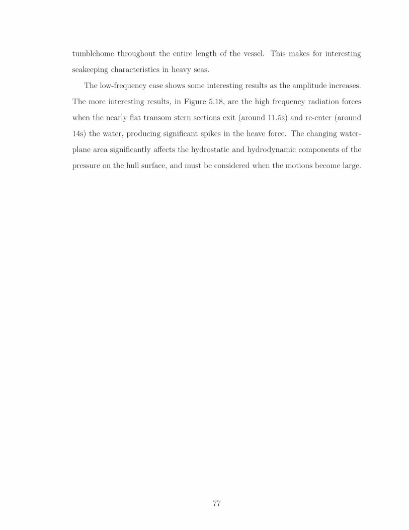
tumblehome throughout the entire length of the vessel. This makes for interesting
seakeeping characteristics in heavy seas.
The low-frequency case shows some interesting results as the amplitude increases.
The more interesting results, in Figure 5.18, are the high frequency radiation forces
when the nearly flat transom stern sections exit (around 11.5s) and re-enter (around
14s) the water, producing significant spikes in the heave force. The changing water-
plane area significantly affects the hydrostatic and hydrodynamic components of the
pressure on the hull surface, and must be considered when the motions become large.
77

Figure 5.16: Views of m5613 (ONR Tumblehome) Hull
78

-4e+06
-3e+06
-2e+06
-1e+06
0
1e+06
2e+06
3e+06
4e+06
5e+06
25 30 35 40 45 50 55
F3
/ am
p [N
/deg
]
F-HS 1.0 degF-HS 2.5 degF-HS 5.0 deg
F-RAD 1.0 degF-RAD 2.5 degF-RAD 5.0 deg
-6e+08
-4e+08
-2e+08
0
2e+08
4e+08
6e+08
25 30 35 40 45 50 55
F5
/ am
p [N
m/d
eg]
Time [s]
F-HS 1.0 degF-HS 2.5 degF-HS 5.0 deg
F-RAD 1.0 degF-RAD 2.5 degF-RAD 5.0 deg
Figure 5.17: m5613 Forced Pitch, ω = 0.3831rad/s
-6e+06
-4e+06
-2e+06
0
2e+06
4e+06
6e+06
10 12 14 16 18 20
F3
/ am
p [N
/deg
]
F-HS 1.0 degF-HS 2.5 degF-HS 5.0 deg
F-RAD 1.0 degF-RAD 2.5 degF-RAD 5.0 deg
-6e+08
-4e+08
-2e+08
0
2e+08
4e+08
6e+08
10 12 14 16 18 20
F5
/ am
p [N
m/d
eg]
Time [s]
F-HS 1.0 degF-HS 2.5 degF-HS 5.0 deg
F-RAD 1.0 degF-RAD 2.5 degF-RAD 5.0 deg
Figure 5.18: m5613 Forced Pitch, ω = 1.1000rad/s
79

CHAPTER VI
Free Motions
6.1 Nonlinear Equations of Motion
The hydrodynamic problem and rigid body equations of motion are solved si-
multaneously in the time-domain. The nonlinear equations of motion described in
Chapter II must be validated. Small amplitude waves can be used to excite the body,
which is now free to move. The type of ramp function used to evolve the free surface
(which begins by being completely calm) will affect the resulting motions. Typically,
a ramp over at least three periods is used for free motion problems. Several periods
later, the body starts to settle into sinusoidal motion and an amplitude and phase
can be determined.
The first model used for comparison is the Series-60 hull form with a block coef-
ficient CB = 0.70. The particulars can be found in Table 5.1. The vessel is exposed
to regular head seas, and will begin to surge, heave, and pitch. The current method
is compared to the strip theory and SWAN codes from MIT, as described earlier
and available in Nakos (1990), and experimental results from Gerritsma et al. (1974).
The surge results are not available because the model was restrained in surge, so only
heave and pitch are shown in Figures 6.1 and 6.2.
The current method shows good agreement, except for over-estimating the reso-
nant peak in heave. This may be related to inaccuracies in the hydrodynamic coupling
80

0
0.2
0.4
0.6
0.8
1
1.2
1.4
1.6
1.8
0.4 0.6 0.8 1 1.2 1.4 1.6
Am
plitu
de [m
/a]
Series-60 (CB=0.7) Heave Response Amplitude Operator, Fn=0.2
Current MethodStrip Theory
SWAN-NakosGerritsma Exp.
-150-100-50
0 50
100 150
0.4 0.6 0.8 1 1.2 1.4 1.6
Pha
se [d
eg]
L / λ
Figure 6.1: Series-60 (CB=0.7) Heave RAO in Head Seas, Fn = 0.2
terms, as discussed in Chapter V. The pitch motions are predicted very accurately,
showing better agreement than the SWAN code. It also seems that the pitch peak
has been shifted in the right direction using the current method, as compared to the
linear strip theory.
An extensive comparison of experimental and computational results for this Series-
60 hull is available in Bailey et al. (2001), including the hydrodynamic coefficients,
exciting forces, and response amplitude operators.
Typically, experimental results for free motions are limited to the vertical plane,
or surge, heave, and pitch. The remaining horizontal plane motions, namely sway and
yaw, have no restoring mechanisms and viscosity is very important. This is especially
true for the cases with forward speed, where the vessel would drift off course if it
weren’t restrained in sway and/or yaw. With that in mind, the remaining degrees-
of-freedom may be validated by comparing to linear theory.
81

0
1
2
3
4
5
6
7
8
0.4 0.6 0.8 1 1.2 1.4 1.6
Am
plitu
de [r
ad L
/a]
Series-60 (CB=0.7) Pitch Response Amplitude Operator, Fn=0.2
Current MethodStrip Theory
SWAN-NakosGerritsma Exp.
-150-100-50
0 50
100 150
0.4 0.6 0.8 1 1.2 1.4 1.6
Pha
se [d
eg]
L / λ
Figure 6.2: Series-60 (CB=0.7) Pitch RAO in Head Seas, Fn = 0.2
The next series of results are for the S-175 containership in regular waves with and
without forward speed. SHIPMO, developed by Beck and Troesch (1989), is the six
degree-of-freedom linear strip theory code used as a comparison. The current method,
Ogilvie-Tuck approximation, and the momentum formulation results are computed
and compared. The Ogilvie-Tuck approximation is the same method as described in
Chapter V and the momentum formulation is described in Appendix A.
The current method and its two alternatives are subject to exactly the same
boundary conditions and numerical schemes, differing only in how they treat the
speed-dependent components of the problem. An extensive set of test parameters
are used, including wave heading angles around the entire ship at increments or 45o,
forward speeds of Fn = 0.0, 0.2, and absolute wavelengths of from L/3 to 5L.
Figures 6.3 through 6.5 show the responses for head seas. The zero-speed results,
shown in blue, are nearly identical. The forward speed results show fairly good
82

0
0.1
0.2
0.3
0.4
0.5
0.6
0.7
0.8
0.9
0 0.5 1 1.5 2 2.5 3
Am
plitu
de [m
/m]
S-175 Surge Response Amplitude Operators
Fn=0.0 Current MethodFn=0.0 Momentum
Fn=0.0 Ogilvie-TuckFn=0.0 SHIPMO
Fn=0.2 Current MethodFn=0.2 Momentum
Fn=0.2 Ogilvie-TuckFn=0.2 SHIPMO
-150-100-50
0 50
100 150
0 0.5 1 1.5 2 2.5 3
Pha
se [d
eg]
L / λ
Figure 6.3: S-175 Surge RAO in Head Seas
agreement between all the methods, except at the resonant peaks of heave and pitch.
The momentum formulation overestimates both of the peaks. The current method,
using direct pressure integration, overestimates the peak heave motions. Using the
Ogilvie-Tuck approach highlights the difference between the two: the treatment of
speed-dependent terms.
Figures 6.6 through 6.11 show a more interesting case of stern-quartering seas,
where all six degrees-of-freedom are excited and unrestrained. The surge, heave, roll,
and pitch motions agree very well. The sway and yaw, in Figures 6.7 and 6.11,
show some significant differences. This is due to the fact that the current method is
a time-domain initial boundary value problem. The viscous corrections and simple
controllers for sway and yaw motions should not affect the motions too significantly.
However, any differences introducing during the startup or ramping phase will prop-
agate in time, and affect the resulting long-term responses. The horizontal modes
83

0
0.2
0.4
0.6
0.8
1
1.2
1.4
1.6
1.8
0 0.5 1 1.5 2 2.5 3
Am
plitu
de [m
/m]
S-175 Heave Response Amplitude Operators
Fn=0.0 Current MethodFn=0.0 Momentum
Fn=0.0 Ogilvie-TuckFn=0.0 SHIPMO
Fn=0.2 Current MethodFn=0.2 Momentum
Fn=0.2 Ogilvie-TuckFn=0.2 SHIPMO
-150-100-50
0 50
100 150
0 0.5 1 1.5 2 2.5 3
Pha
se [d
eg]
L / λ
Figure 6.4: S-175 Heave RAO in Head Seas
0
0.5
1
1.5
2
2.5
0 0.5 1 1.5 2 2.5 3
Am
plitu
de [d
eg/m
]
S-175 Pitch Response Amplitude Operators
Fn=0.0 Current MethodFn=0.0 Momentum
Fn=0.0 Ogilvie-TuckFn=0.0 SHIPMO
Fn=0.2 Current MethodFn=0.2 Momentum
Fn=0.2 Ogilvie-TuckFn=0.2 SHIPMO
-150-100-50
0 50
100 150
0 0.5 1 1.5 2 2.5 3
Pha
se [d
eg]
L / λ
Figure 6.5: S-175 Pitch RAO in Head Seas
84

0
0.1
0.2
0.3
0.4
0.5
0.6
0.7
0.8
0.9
1
0 0.5 1 1.5 2 2.5 3
Am
plitu
de [m
/m]
S-175 Surge Response Amplitude Operators
Fn=0.0 Current MethodFn=0.0 Momentum
Fn=0.0 SHIPMOFn=0.2 Current Method
Fn=0.2 MomentumFn=0.2 SHIPMO
-150-100-50
0 50
100 150
0 0.5 1 1.5 2 2.5 3
Pha
se [d
eg]
L / λ
Figure 6.6: S-175 Surge RAO in Stern Quartering Seas
have no restoring mechanisms. Any differences are difficult to control and may lead
to significantly different motions.
The remaining runs (for following, beam, and bow quartering seas) are available in
Appendix D. The direct pressure and momentum formulations agree fairly well. The
agreement with SHIPMO must be considered on a case-by-case basis. However, the
momentum formulation, as derived, may not be suitable for large amplitude motions.
This is briefly discussed in Appendix A
85

0
0.1
0.2
0.3
0.4
0.5
0.6
0.7
0.8
0.9
0 0.5 1 1.5 2 2.5 3
Am
plitu
de [m
/m]
S-175 Sway Response Amplitude Operators
-150-100-50
0 50
100 150
0 0.5 1 1.5 2 2.5 3
Pha
se [d
eg]
L / λ
Figure 6.7: S-175 Sway RAO in Stern Quartering Seas
0
0.1
0.2
0.3
0.4
0.5
0.6
0.7
0.8
0.9
1
0 0.5 1 1.5 2 2.5 3
Am
plitu
de [m
/m]
S-175 Heave Response Amplitude Operators
-150-100-50
0 50
100 150
0 0.5 1 1.5 2 2.5 3
Pha
se [d
eg]
L / λ
Figure 6.8: S-175 Heave RAO in Stern Quartering Seas
86
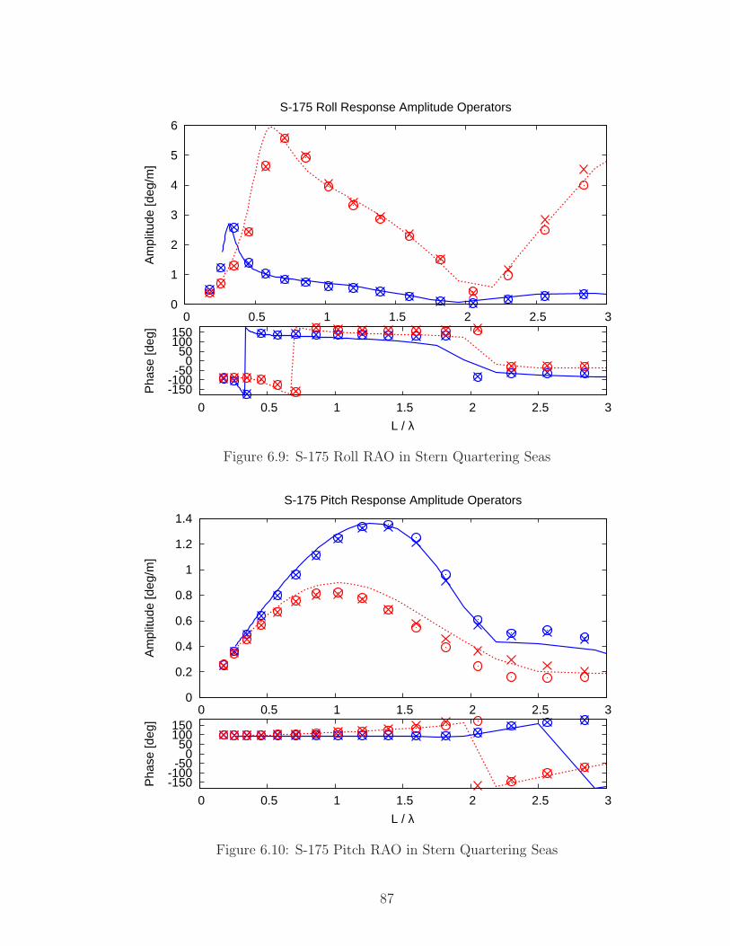
0
1
2
3
4
5
6
0 0.5 1 1.5 2 2.5 3
Am
plitu
de [d
eg/m
]
S-175 Roll Response Amplitude Operators
-150-100-50
0 50
100 150
0 0.5 1 1.5 2 2.5 3
Pha
se [d
eg]
L / λ
Figure 6.9: S-175 Roll RAO in Stern Quartering Seas
0
0.2
0.4
0.6
0.8
1
1.2
1.4
0 0.5 1 1.5 2 2.5 3
Am
plitu
de [d
eg/m
]
S-175 Pitch Response Amplitude Operators
-150-100-50
0 50
100 150
0 0.5 1 1.5 2 2.5 3
Pha
se [d
eg]
L / λ
Figure 6.10: S-175 Pitch RAO in Stern Quartering Seas
87
0
0.2
0.4
0.6
0.8
1
1.2
0 0.5 1 1.5 2 2.5 3
Am
plitu
de [d
eg/m
]
S-175 Yaw Response Amplitude Operators
-150-100-50
0 50
100 150
0 0.5 1 1.5 2 2.5 3
Pha
se [d
eg]
L / λ
Figure 6.11: S-175 Yaw RAO in Stern Quartering Seas
88

CHAPTER VII
Discussion
7.1 Conclusions
The body-exact strip theory presented shows very encouraging results. Conver-
gence tests have been carried out, as well as small and large amplitude validations for
the two-dimensional problem. The strip theory has been demonstrated to give good
predictions, with a few exceptions. Some of these poor comparisons might be im-
proved if better techniques were used to account for the interaction between sections,
which becomes important with forward speed.
The computation speed is very fast, executing near real-time (or better) on a
high-end desktop PC. The numerical methods still have room for improvement as far
as speed is concerned. The single most intensive portion of the code is the influence
matrix inversion. This is needed for the two-dimensional boundary value problem(s)
and the influence matrix when using Radial Basis Functions. The latter has the most
room for improvements.
The robust capabilities of this method make it a good candidate for large motion
simulations of any hull form that meets the slender-body requirements. Loading the
hull offsets is straightforward, and a wide range of analyses is available.
89
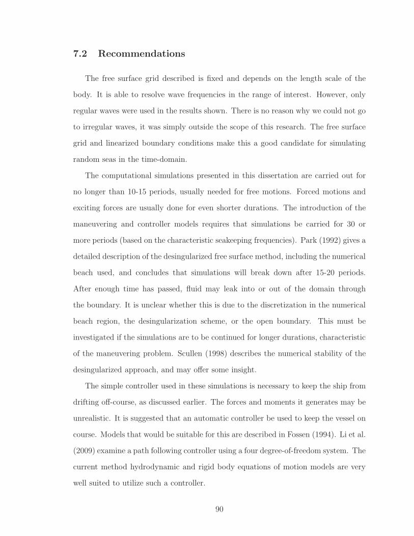
7.2 Recommendations
The free surface grid described is fixed and depends on the length scale of the
body. It is able to resolve wave frequencies in the range of interest. However, only
regular waves were used in the results shown. There is no reason why we could not go
to irregular waves, it was simply outside the scope of this research. The free surface
grid and linearized boundary conditions make this a good candidate for simulating
random seas in the time-domain.
The computational simulations presented in this dissertation are carried out for
no longer than 10-15 periods, usually needed for free motions. Forced motions and
exciting forces are usually done for even shorter durations. The introduction of the
maneuvering and controller models requires that simulations be carried for 30 or
more periods (based on the characteristic seakeeping frequencies). Park (1992) gives a
detailed description of the desingularized free surface method, including the numerical
beach used, and concludes that simulations will break down after 15-20 periods.
After enough time has passed, fluid may leak into or out of the domain through
the boundary. It is unclear whether this is due to the discretization in the numerical
beach region, the desingularization scheme, or the open boundary. This must be
investigated if the simulations are to be continued for longer durations, characteristic
of the maneuvering problem. Scullen (1998) describes the numerical stability of the
desingularized approach, and may offer some insight.
The simple controller used in these simulations is necessary to keep the ship from
drifting off-course, as discussed earlier. The forces and moments it generates may be
unrealistic. It is suggested that an automatic controller be used to keep the vessel on
course. Models that would be suitable for this are described in Fossen (1994). Li et al.
(2009) examine a path following controller using a four degree-of-freedom system. The
current method hydrodynamic and rigid body equations of motion models are very
well suited to utilize such a controller.
90
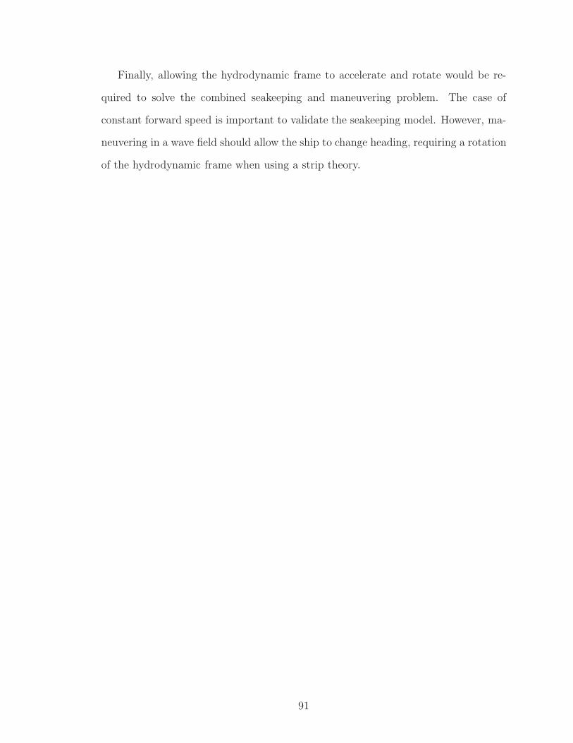
Finally, allowing the hydrodynamic frame to accelerate and rotate would be re-
quired to solve the combined seakeeping and maneuvering problem. The case of
constant forward speed is important to validate the seakeeping model. However, ma-
neuvering in a wave field should allow the ship to change heading, requiring a rotation
of the hydrodynamic frame when using a strip theory.
91

APPENDICES
92

APPENDIX A
Momentum Formulation
The momentum formulation requires solving the φ problem first. However, the
resulting formulas do not calculate the pressure on the body to find the forces and
moments. This was derived as an alternative to the direct pressure integration for the
“swimming fish” problem by Newman and Wu (1973). The derivation, including a
free surface, is shown in Sclavounos (2008). The main difference is the use of z = 0 for
the free surface conditions, instead of the weak scatterer assumption by Sclavounos.
For the two-dimensional problem, the dynamic sectional forces can be approximated
by
fDY Ni =
∫
CH
pDY NNidl (A.1)
fDY Ni = −ρ d
dt
∫
CH
φNidl − ρ
∫
CWP
(gζI +∂φI
∂t)Nidl (A.2)
where CWP is the exact waterplane contour intersecting the body at that section
For the strip theory approximation, the total dynamic forces and moments can be
93

written in terms of the perturbation potential
FDY Ni = −ρ
∫
L
dx[∂
∂t
∫
CH
φNidl−Uo∂
∂x
∫
CH
φNidl+
∫
CWP
(gζI+∂φI
∂t−Uo
∂φI
∂x)Nidl] (A.3)
where the sectional integrals are functions of both time and the longitudinal direction
(or t and x), so partial derivates must be used.
The speed dependent component of the force is apparent in the second term.
Numerically, this is much simpler than approximating ∂φ∂x
at every node. A drawback
of the momentum approach is that the pressure distribution is not known.
The momentum formulation works well for small amplitude motions. When the
motions get large, and the sectional areas change, the evaluation of the time-derivative
(or x-derivative if the sections change shape rapidly along the length) becomes prob-
lematic. The partial derivatives are brought outside of the sectional integrals, and
now the changing integrals along the contour maybe be a function of time, t (or x)
themselves.
As an example of this, a simple two-dimensional circular section is used. Oscillat-
ing at a frequency ω(R/g)0.5 = 1.0, and a radius R = 10m, a range of heave amplitudes
are used and the added mass and damping are plotted versus amplitude. The results
are presented in Figure A.1, where a′33 = a33/(ρA) and b′33 = b33(R/2)0.5/(ρA). The
pressure and momentum results are presented, along with experimental results of
Vugts (1968). The experimental results were done for small amplitudes, and compare
well with linear theory. The linear result is plotted as a constant, independent of
motion amplitude.
The results compare well up to about 20% of the radius. This might still be con-
sidered a “small” amplitude, especially for the a circular section where the waterplane
intersection does not change significantly. As expected, the added mass and damping
decrease with amplitude when compared to linear theory. However, the heave damp-
94

0.2
0.3
0.4
0.5
0.6
0.7
0.8
0 1 2 3 4 5 6 7
a’33
, b’ 3
3
Heave Amplitude [m] (R=10m)
Large Amplitude Comparison: Pressure and Momentum Formulations
a’33 - Pressurea’33 - Momentuma’33 - Vugts Exp.
b’33 - Pressureb’33 - Momentumb’33 - Vugts Exp.
Figure A.1: Pressure and Momentum Comparison - Large Amplitude Heaving Circu-lar Section
ing coefficient, b33, seems to change much more significantly with the momentum
approach. This emphasizes a possible problem with the method, as derived.
As the amplitude of motion increases, the force time-series should become more
nonlinear and the linear coefficients are no longer sufficient to describe them. Fig-
ures A.2 through A.4 show the total hydrodynamic heave force acting on the two-
dimesnional section with increasing amplitudes of motion (1.0, 4.0, and 7.0m, where
the cylinder radius R = 10.0m). As can be seen for the small amplitude case in Figure
A.2, the methods agree well and may accurately be described using linear coefficients.
However, as the amplitude increases, the force time-series comparisons begin to show
significant differences. This confirms the results of the Fourier transform of the first-
order terms, shown in Figure A.1. The momentum formulation, as derived, may have
some difficulties when the amplitude of motion becomes significant. Further research
is needed to investigate these differences.
95
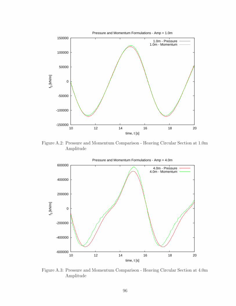
-150000
-100000
-50000
0
50000
100000
150000
10 12 14 16 18 20
f 3 [k
N/m
]
time, t [s]
Pressure and Momentum Formulations - Amp = 1.0m
1.0m - Pressure1.0m - Momentum
Figure A.2: Pressure and Momentum Comparison - Heaving Circular Section at 1.0mAmplitude
-600000
-400000
-200000
0
200000
400000
600000
10 12 14 16 18 20
f 3 [k
N/m
]
time, t [s]
Pressure and Momentum Formulations - Amp = 4.0m
4.0m - Pressure4.0m - Momentum
Figure A.3: Pressure and Momentum Comparison - Heaving Circular Section at 4.0mAmplitude
96
-1.5e+06
-1e+06
-500000
0
500000
1e+06
1.5e+06
10 12 14 16 18 20
f 3 [k
N/m
]
time, t [s]
Pressure and Momentum Formulations - Amp = 7.0m
7.0m - Pressure7.0m - Momentum
Figure A.4: Pressure and Momentum Comparison - Heaving Circular Section at 7.0mAmplitude
97

APPENDIX B
Influence Matrices for Two-Dimensional Problem
In the two-dimensional boundary value problem, we use a source distribution to
satisfy the free surface and body boundary conditions. The free surface is modeled
using desingularized sources, while the body is modeled using constant strength flat
panels. In this section, the influence of a source point or panel on any field point is
derived. This includes the influence to get the potential and it’s derivatives in space at
any field point. Along the way, common variables will be introduced that frequently
appear in the derivations. These are intended to make more compact formulas, and
are also helpful in terms of computational effort. The variables can be computed for
each source influence on a field point and then used to determine the proper influence
coefficients. It reduces the computational effort in setting up the influence matrices.
The Rankine source Green function used in the two-dimensional problem is
G(xi; ξj) = ln r is the Green function (B.1)
xi = (yi, zi) is the field point (B.2)
ξj = (ηj, ζj) is the source point (B.3)
r = |xi − ξj | is the distance between the points (B.4)
98
Now, we derive the influence of one source point on one field point, so the in-
dices can be dropped. This simplifies the mathematical notation in the following
derivations. The following terms are also defined
∆y = y − η (B.5)
∆z = z − ζ (B.6)
N = (N2, N3) is the two-dimensional unit normal (B.7)
r =√
∆y2 + ∆z2 (B.8)
where N will be the unit normal on the field point. It is well-defined on the body,
and equal to (0, 1) on the linearized free surface.
The derivation for desingularized point sources and panels is slightly different. Let
GS be the point source influence, and GP be the line source influence on a panel of
length L.
GS = ln r (B.9)
GP =∫
L
ln rdl (B.10)
The space derivatives are found by simply taking the partial derivatives with respect
to the variables y, z. The notation will be such that GSy, GSz are the y− and z−
partial derivatives of GS. Second derivatives follow a similar notation. The gradient
of GP , for example, would be given by ∇GP = (GPy, GPz).
First, we derive the influence of a desingularized point source. Finding the po-
tential from the influence is trivial, given by Eqn. B.9. Its derivatives are given
99

by
GSy =∆y
r2(B.11)
GSz =∆z
r2(B.12)
GSyy = −GSzz =∆z2 − ∆y2
r4(B.13)
GSyz = GSzy =−2∆y∆z
r4(B.14)
The derivation of the constant strength flat panel, or line source, influence is a
bit more cumbersome. Since the integrals are along the panel, we introduce a new
variable t that is tangent to the panel in the yz − plane, in a direction of negative
rotation about x, using the right-hand rule. The integration is now in one space
dimension, and goes from −L/2 to L/2, as shown in Figure B.1. The variables η, ζ
have been parameterized by the single variable t, such that
η∗ = η − tN3 (B.15)
ζ∗ = ζ + tN2 (B.16)
GP =
L/2∫
−L/2
1
2ln([y − (η − tN3)]
2 + [z − (ζ + tN2)]2)dt (B.17)
GP = L(c1 + c2
4− 1 − ln 2) + a2c0 + a1
c1 − c22
(B.18)
100

z
y
i
i+1
N
t
t=L/2
t=-L/2
( η , ζ )
N
N2
N3
Figure B.1: Parameterization of panel integrals using t, the tangent variable
where a1 = −∆yN3 + ∆zN2
a2 = −∆yN2 − ∆zN3
b1 = r2 +L2
4
b2 = a1L
c0 = arctan(L2− a1
a2) + arctan(
L2
+ a1
a2)
c1 = ln(4(r2 + a1L) + L2)
c2 = ln(4(r2 − a1L) + L2)
And the derivatives are given by
GPy = −N3c1 − c2
2−N2c0 (B.19)
GPz = N2c1 − c2
2−N3c0 (B.20)
GPyy = −GPzz = L∆z2 − ∆y2 + L2
4(N2
3 −N22 )
(b1 + b2)(b1 − b2)(B.21)
GPyz = GPzy = 2L−L2
4N3N2 − ∆y∆z
(b1 + b2)(b1 − b2)(B.22)
101
Finally, the limiting case of x = ξ must be examined. This is not an issue in the
point source derivation, since they are desingularized. For the panel influence, we
observe the following when considering a panel’s influence on itself: ∆y = ∆z = r =
a1 = a2 = b2 = 0 and c1 = c2. This simplifies the coefficients, and we must be careful
of the arctan terms in c0. Taking the limit as x → ξ (from the fluid domain towards
the boundary), we get c0 = π, and the following coefficients for the panel’s influence
on itself
GPy = −πN2 (B.23)
GPz = −πN3 (B.24)
(B.25)
which results in the −π term in Eqn. 3.7, the special case of the panel’s influence on
itself.
102

APPENDIX C
Validation of Influence Matrices
The velocity potential for a circular section translating vertically an infinite fluid
is given by
φ = −W R2z
y2 + z2(C.1)
where W is the vertical velocity, R is the radius, and y, z are the location of a point
in the fluid domain, in the body-axis system. As a preliminary check, the influence
matrices derived in Appendix B can be verified. The velocity potential and it’s
derivatives using the influence matrices can be compared to the analytic solutions.
The velocity potential and its derivatives in space (first and second) are compared.
The panel method, desingularized method, and analytic solutions are compared. Fig-
ures C.1 through C.3 show the potential, its gradient, and gradient of the gradient.
The values are plotted against the location on the body, in radians, measured clock-
wise from the positive z−axis. Note that Figure C.3 only shows φyy and φyz, since the
following relations hold for the two-dimensional potential: φzz = −φyy and φzy = φyz.
The potential and its gradient, shown in Figures C.1 and C.2, match exactly using
all three solutions. This validates the influence matrices that were derived earlier. The
second space derivatives are needed for the body boundary conditions of the radiation
acceleration potential, as can be seen in Eqn. (2.65). Determining these values using
103

-25
-20
-15
-10
-5
0
5
10
15
20
25
0 1 2 3 4 5 6 7
φ [m
2 /s]
Node location relative to vertical [rad]
φ - Velocity Potential on Body
PanelDesingularized
Analytic
Figure C.1: φ on Body, Deeply Submerged Heaving Circular Cylinder
-2.5
-2
-1.5
-1
-0.5
0
0.5
1
1.5
2
2.5
0 1 2 3 4 5 6 7
φ y,φ
z [m
/s]
Node location relative to vertical [rad]
φy,φz - Velocity on Body
φy Panelφy Desingularized
φy Analyticφz Panel
φz Desingularizedφz Analytic
Figure C.2: φy, φz on Body, Deeply Submerged Heaving Circular Cylinder
104

-0.5
-0.4
-0.3
-0.2
-0.1
0
0.1
0.2
0.3
0.4
0.5
0 1 2 3 4 5 6 7
φ yy,
φ yz
[1/s
]
Node location relative to vertical [rad]
φyy,φyz - Grad(Velocity) on Body
φyy Panelφyy Desingularized
φyy Analyticφyz Panel
φyz Desingularizedφyz Analytic
Figure C.3: φyy, φyz on Body, Deeply Submerged Heaving Circular Cylinder
the influence matrices is shown in Figure C.3, and there are significant differences
when using the panel method. The influence matrices have been checked for errors,
and are correct. The reason for this difference appears to be inherent to the panel
method itself. Each individual panel is flat and has a constant source strength along
its length. As partial derivatives are taken and found in the limit of the panel control
point, or midpoint, the panel method will not provide good results for the gradient
of the fluid velocity. If a field point somewhere off the panel were chosen instead, the
solution would improve. An example of this can be seen in Figure C.4, plotting the
second space derivates as a function of the radial distance from the control point. In
this case, the panel size is 0.42m and R = 10m, and the solutions start to diverge for
values of r/R < 0.05, or r < 0.5m. This suggests that using the influence matrices to
find ∇(∇φ) in the vicinity of the panel will yield bad results. As this distance of the
field point from the panel increases, the solution approaches that of the desingularized
method (assuming the desingularized point is on the “inside” of the body, while the
105

-0.1
-0.05
0
0.05
0.1
0.15
0.2
0.25
0.3
0.001 0.01 0.1 1
φ yy,
φ yz
[1/s
]
Radial distance from control point, r/R
φyy,φyz - Grad(Fluid Velocity)
φyy Panelφyy Desingularized
φyy Analyticφyz Panel
φyz Desingularizedφyz Analytic
Figure C.4: φyy, φyz Comparison at Field Points in Fluid Domain, in Radial Directionfrom Body, Panel Length dl = 0.042R
field point is in the fluid domain).
As an alternative solution, we use the panel method solution of the gradient of
phi, φy, φz, and numerically differentiate it between adjacent panels to estimate φyt
and φzt, where the t subscript indicates a partial derivative in the tangential direction.
The results can then be transformed back into φyy, φyz coordinates, as needed. Figure
C.5 shows the improved results.
This numerical approach is accurate as long as the angle between panels does not
change significantly. In most ship stations, there will only be a few “corners” (at
most) where this may not work too well. Overall, since there will be 50-100 panels on
a section, it will not significantly affect the solution, since this value is a higher order
component in the boundary value problem and only problematic for small fraction of
points.
106

-0.5
-0.4
-0.3
-0.2
-0.1
0
0.1
0.2
0.3
0.4
0.5
0 1 2 3 4 5 6 7
φ yy,
φ yz
[1/s
]
Node location relative to vertical [rad]
φyy,φyz - Grad(Velocity) on Body, alternative
φyy Panelφyy Desingularized
φyy Analyticφyz Panel
φyz Desingularizedφyz Analytic
Figure C.5: Corrected φyy, φyz on Body
107

APPENDIX D
S-175 Response Amplitude Operators
The remaining cases of S-175 response validations are presented, completing the
set of results shown in Chapter VI.
Following Seas
Beam Seas
Bow Quartering Seas
108

0
0.2
0.4
0.6
0.8
1
1.2
1.4
1.6
1.8
0 0.5 1 1.5 2 2.5 3
Am
plitu
de [m
/m]
S-175 Surge Response Amplitude Operators
Fn=0.0 Current MethodFn=0.0 Momentum
Fn=0.0 SHIPMOFn=0.2 Current Method
Fn=0.2 MomentumFn=0.2 SHIPMO
-150-100-50
0 50
100 150
0 0.5 1 1.5 2 2.5 3
Pha
se [d
eg]
L / λ
Figure D.1: S-175 Surge RAO in Following Seas
0
0.1
0.2
0.3
0.4
0.5
0.6
0.7
0.8
0.9
1
0 0.5 1 1.5 2 2.5 3
Am
plitu
de [m
/m]
S-175 Heave Response Amplitude Operators
-150-100-50
0 50
100 150
0 0.5 1 1.5 2 2.5 3
Pha
se [d
eg]
L / λ
Figure D.2: S-175 Heave RAO in Following Seas
109

0
0.2
0.4
0.6
0.8
1
1.2
1.4
0 0.5 1 1.5 2 2.5 3
Am
plitu
de [d
eg/m
]
S-175 Pitch Response Amplitude Operators
-150-100-50
0 50
100 150
0 0.5 1 1.5 2 2.5 3
Pha
se [d
eg]
L / λ
Figure D.3: S-175 Pitch RAO in Following Seas
0
0.01
0.02
0.03
0.04
0.05
0.06
0.07
0.08
0 0.5 1 1.5 2 2.5 3
Am
plitu
de [m
/m]
S-175 Surge Response Amplitude Operators
Fn=0.0 Current MethodFn=0.0 Momentum
Fn=0.0 SHIPMOFn=0.2 Current Method
Fn=0.2 MomentumFn=0.2 SHIPMO
-150-100-50
0 50
100 150
0 0.5 1 1.5 2 2.5 3
Pha
se [d
eg]
L / λ
Figure D.4: S-175 Surge RAO in Beam Seas
110

0.4
0.5
0.6
0.7
0.8
0.9
1
0 0.5 1 1.5 2 2.5 3
Am
plitu
de [m
/m]
S-175 Sway Response Amplitude Operators
-150-100-50
0 50
100 150
0 0.5 1 1.5 2 2.5 3
Pha
se [d
eg]
L / λ
Figure D.5: S-175 Sway RAO in Beam Seas
0.5
0.6
0.7
0.8
0.9
1
1.1
1.2
1.3
1.4
1.5
0 0.5 1 1.5 2 2.5 3
Am
plitu
de [m
/m]
S-175 Heave Response Amplitude Operators
-150-100-50
0 50
100 150
0 0.5 1 1.5 2 2.5 3
Pha
se [d
eg]
L / λ
Figure D.6: S-175 Heave RAO in Beam Seas
111
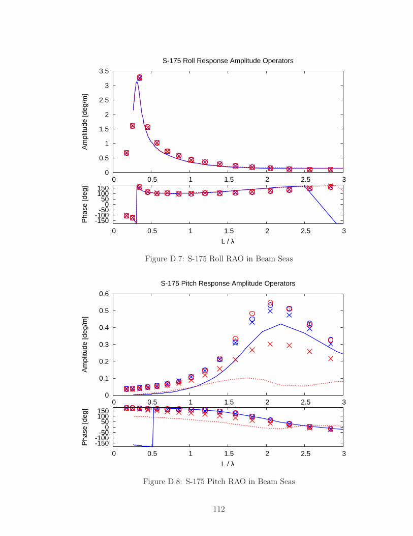
0
0.5
1
1.5
2
2.5
3
3.5
0 0.5 1 1.5 2 2.5 3
Am
plitu
de [d
eg/m
]
S-175 Roll Response Amplitude Operators
-150-100-50
0 50
100 150
0 0.5 1 1.5 2 2.5 3
Pha
se [d
eg]
L / λ
Figure D.7: S-175 Roll RAO in Beam Seas
0
0.1
0.2
0.3
0.4
0.5
0.6
0 0.5 1 1.5 2 2.5 3
Am
plitu
de [d
eg/m
]
S-175 Pitch Response Amplitude Operators
-150-100-50
0 50
100 150
0 0.5 1 1.5 2 2.5 3
Pha
se [d
eg]
L / λ
Figure D.8: S-175 Pitch RAO in Beam Seas
112

0
0.01
0.02
0.03
0.04
0.05
0.06
0.07
0 0.5 1 1.5 2 2.5 3
Am
plitu
de [d
eg/m
]
S-175 Yaw Response Amplitude Operators
-150-100-50
0 50
100 150
0 0.5 1 1.5 2 2.5 3
Pha
se [d
eg]
L / λ
Figure D.9: S-175 Yaw RAO in Beam Seas
0
0.1
0.2
0.3
0.4
0.5
0.6
0.7
0 0.5 1 1.5 2 2.5 3
Am
plitu
de [m
/m]
S-175 Surge Response Amplitude Operators
Fn=0.0 Current MethodFn=0.0 Momentum
Fn=0.0 SHIPMOFn=0.2 Current Method
Fn=0.2 MomentumFn=0.2 SHIPMO
-150-100-50
0 50
100 150
0 0.5 1 1.5 2 2.5 3
Pha
se [d
eg]
L / λ
Figure D.10: S-175 Surge RAO in Bow Quartering Seas
113

0
0.1
0.2
0.3
0.4
0.5
0.6
0.7
0 0.5 1 1.5 2 2.5 3
Am
plitu
de [m
/m]
S-175 Sway Response Amplitude Operators
-150-100-50
0 50
100 150
0 0.5 1 1.5 2 2.5 3
Pha
se [d
eg]
L / λ
Figure D.11: S-175 Sway RAO in Bow Quartering Seas
0
0.2
0.4
0.6
0.8
1
1.2
1.4
1.6
1.8
2
0 0.5 1 1.5 2 2.5 3
Am
plitu
de [m
/m]
S-175 Heave Response Amplitude Operators
-150-100-50
0 50
100 150
0 0.5 1 1.5 2 2.5 3
Pha
se [d
eg]
L / λ
Figure D.12: S-175 Heave RAO in Bow Quartering Seas
114

0
0.5
1
1.5
2
2.5
3
0 0.5 1 1.5 2 2.5 3
Am
plitu
de [d
eg/m
]
S-175 Roll Response Amplitude Operators
-150-100-50
0 50
100 150
0 0.5 1 1.5 2 2.5 3
Pha
se [d
eg]
L / λ
Figure D.13: S-175 Roll RAO in Bow Quartering Seas
0 0.2 0.4 0.6 0.8
1 1.2 1.4 1.6 1.8
2 2.2
0 0.5 1 1.5 2 2.5 3
Am
plitu
de [d
eg/m
]
S-175 Pitch Response Amplitude Operators
-150-100-50
0 50
100 150
0 0.5 1 1.5 2 2.5 3
Pha
se [d
eg]
L / λ
Figure D.14: S-175 Pitch RAO in Bow Quartering Seas
115

0
0.05
0.1
0.15
0.2
0.25
0.3
0.35
0.4
0.45
0.5
0 0.5 1 1.5 2 2.5 3
Am
plitu
de [d
eg/m
]
S-175 Yaw Response Amplitude Operators
-150-100-50
0 50
100 150
0 0.5 1 1.5 2 2.5 3
Pha
se [d
eg]
L / λ
Figure D.15: S-175 Yaw RAO in Bow Quartering Seas
116

BIBLIOGRAPHY
117
BIBLIOGRAPHY
Bailey, P. A., D. A. Hudson, W. G. Price, and P. Temarel (2001). Comparisonsbetween theory and experiment in a seakeeping validation study. TransactionsRINA.
Bailey, P. A., W. G. Price, and P. Temarel (1998). A unified mathematical modeldescribing the manoeuvring of a ship travelling in a seaway. Transactions RINA 140,131–149.
Beck, R. F. (1989). Ship responses to regular waves. In Principles of Naval Architec-ture, Volume III, Chapter 8, pp. 41–83. SNAME.
Beck, R. F. (1999). Fully nonlinear water wave computations using a desingularizedeuler-lagrange time-domain approach. In Nonlinear Water Wave Interaction, pp.1–58. WIT Press.
Beck, R. F., Y. Cao, S. Scorpio, and W. W. Schultz (1994). Nonlinear ship mo-tion computations using the desingularized method. In 20th Symposium on NavalHydrodynamics. National Academies Press.
Beck, R. F. and A. R. Magee (1990). Time-domain analysis for predicting shipmotions. In Symposium on the Dynamics of Marine Vehicles and Structures inWaves, Brunel University, Amsterdam, the Netherlands, pp. 49–65.
Beck, R. F. and A. M. Reed (2001). Modern computational methods for ships in aseaway. Transactions SNAME 109, 1–51.
Beck, R. F. and A. W. Troesch (1989). Documentation and users manual for the com-puter program shipmo. Technical report, The University of Michigan, Departmentof Naval Architecture and Marine Engineering.
Bishop, R. E. D. and W. G. Price (1981). On the use of equilibrium axes and body axesin the dynamics of a rigid ship. Journal of Mechanical Engineering Science 23 (5),243–256.
Buhmann, M. D. (2000). Radial basis functions. Acta Numerica, 1–38.
Cao, Y. (1991). Computation of nonlinear gravity waves by a desingularized boundaryintegral method. Ph. D. thesis, The University of Michigan, Department of NavalArchitecture and Marine Engineering.
118

Cao, Y., W. W. Schultz, and R. F. Beck (1990). Three-dimensional, unsteady compu-tations of nonlinear waves caused by underwater disturbances. In 18th Symposiumon Naval Hydrodynamics, pp. 417–425. National Academies Press.
Cao, Y., W. W. Schultz, and R. F. Beck (1991). Three-dimensional desingularizedboundary integral methods for potential problems. International Journal for Nu-merical Methods in Fluids 12, 785–803.
Clarke, D., P. Gedling, and G. Hine (1983). The application of maneuvering criteriain hull design using linear theory. Transactions RINA, 45–68.
Dawson, C. W. (1977). A practical computer method for solving ship-wave problems.In 2nd International Conference on Numerical Ship Hydrodynamics, Berkeley, Cal-ifornia.
Faltinsen, O. M. and R. Zhao (1991). Numerical predictions of ship motions athigh forward speed. Philosophical Transactions A: Physical Sciences and Engi-neering 334, 241–252.
Fang, M. C., J. H. Luo, and M. L. Lee (2005). A nonlinear mathematical model forship turning circle simulation in waves. Journal of Ship Research 49 (2), 69–79.
Finn, P. J., R. F. Beck, A. W. Troesch, and Y. S. Shin (2003). Nonlinear impactloading in an oblique seaway. Journal of Offshore Mechanics and Arctic Engineer-ing 125 (3), 190–197.
Fossen, T. I. (1991). Nonlinear modelling and control of underwater vehicles. Ph. D.thesis, Norwegian Institute of Technology, Department of Engineering Cybernetics.
Fossen, T. I. (1994). Modeling of marine vehicles. In Guidance and Control of OceanVehicles, Chapter 2, pp. 5–56. John Wiley and Sons.
Fossen, T. I. (2005). A nonlinear unified state-space model for ship maneuvering andcontrol in a seaway. 15 (9), 2717–2746. International Journal of Bifurcation andChaos.
Fossen, T. I. and O. N. Smogeli (2004). Nonlinear time-domain strip theory formu-lation for low-speed manoeuvring and station-keeping. Modeling Identification andControl 25 (4), 201–221.
Gerritsma, J. (1988). Motions, wave loads and added resistance in waves of twowigley hull forms. Delft University of Technology, Shiphydromechanics laboratory,Report 804.
Gerritsma, J. and W. Beukelman (1967). Analysis of the modified strip theory for thecalculation of ship motions and wave bending moments. International ShipbuildingProgress 14 (156), 319–337.
119

Gerritsma, J., W. Beukelman, and C. C. Glansdorp (1974). The effect of beamon the hydrodynamic characteristics of ship hulls. In 10th Symposium on NavalHydrodynamics, Boston, USA.
Himeno, Y. (1981). Prediction of ship roll damping-state of the art. Technical Report239, University of Michigan, Dept. of Naval Architecture and Marine Engineering.
Journee, J. M. (1992). Experiments and calculations on four wigley hullforms,technical report 909. Technical report, Delft University of Technology, ShipHydromechanics Laboratory, Delft, The Netherlands.
Kang, C. G. and I. Y. Gong (1990). A numerical solution method for three-dimensional nonlinear free surface problems. In 18th Symposium on Naval Hy-drodynamics, pp. 427–438. National Academies Press.
Kansa, E. J. (1999). Motivation for using radial basis functions to solve pdes. Tech-nical report, Lawrence Livermore National Laboratory, Livermore, Ca.
Kent, C. P. (2005). A pseudo-spectral method for calculating wave-body interaction us-ing an explicit free-surface formulation. Ph. D. thesis, The University of Michigan,Department of Naval Architecture and Marine Engineering.
Korvin-Kroukovsky, B. V. and W. R. Jacobs (1957). Pitching and heaving motionsof a ship in regular waves. Transactions SNAME 65, 590–632.
Kring, D., Y. Huang, P. Sclavounos, T. Vada, and A. Braathen (1996). Nonlinearship motions and wave-induced loads by a rankine method. In 21st Symposium onNaval Hydrodynamics, pp. 45–63. National Academies Press.
Lee, T. H. (1992). Nonlinear radiation problems for a surface-piercing body. Ph. D.thesis, The University of Michigan, Department of Naval Architecture and MarineEngineering.
Li, Z., J. Sun, and S. Oh (2009). Design, analysis and experimental validation of arobust nonlinear path following controller for marine surface vessels. Automatica.
Lin, W. M. and D. K. P. Yue (1990). Numerical solutions for large-amplitude shipmotions in the time-domain. In 18th Symposium on Naval Hydrodynamics, pp.41–66. National Academies Press.
Longuet-Higgins, M. S. and E. D. Cokelet (1976). The deformation of steep surfacewaves on water. i. a numerical method of computation. In Royal Society of London.Series A: Mathematical and Physical Sciences, Volume 350, pp. 1–26.
Maruo, H. and W. Song (1994). Nonlinear analysis of bow wave breaking and deckwetness of a high-speed ship by the parabolic approximation. In 20th Symposiumon Naval Hydrodynamics. National Academies Press.
120

Nakos, D. and P. D. Sclavounos (1990). Ship motions by a three-dimensional rankinepanel method. In 18th Symposium on Naval Hydrodynamics, pp. 21–40. NationalAcademies Press.
Nakos, D. E. (1990). Ship wave patterns and motions by a three dimensional Rankinepanel method. Ph. D. thesis, Massachusetts Institute of Technology, Department ofOcean Engineering.
Newman, J. N. (1978). The theory of ship motions. Advances in Applied Mechan-ics 18, 221–283.
Newman, J. N. and T. Y. Wu (1973). A generalized slender-body theory for fish-likeforms. Journal of Fluid Mechanics Digital Archive 57 (04), 673–693.
Ogilvie, T. F. and E. O. Tuck (1969). A rational strip theory of ship motions: Parti. Technical Report 013, University of Michigan, Dept. of Naval Architecture andMarine Engineering.
Park, J. H. (1992). The numerical stability of nonlinear floating body calculations.Ph. D. thesis, The University of Michigan, Department of Naval Architecture andMarine Engineering.
Park, J. H. and A. W. Troesch (1992). Numerical modeling of short-time scale non-linear water waves generated by large vertical motions of non-wallsided bodies. In19th Symposium on Naval Hydrodynamics, pp. 143–158. National Academies Press.
Pawlowski, J. (1992). A nonlinear theory of ship motion in waves. In 19th Symposiumon Naval Hydrodynamics, pp. 33–58. National Academies Press.
Salvesen, N., E. O. Tuck, and O. M. Faltinsen (1970). Ship motions and sea loads.Transactions SNAME 78, 250–287.
Sclavounos, P. D. (2008). Nonlinear response modeling of a vessel in steep randomwaves. Personal Correspondence with R. F. Beck.
Sclavounos, P. D., D. C. Kring, Y. Huang, D. A. Mantzaris, S. Kim, and Y. W. Kim(1997). A computational method as an advanced tool of ship hydrodynamic design.Transactions SNAME 105, 378–397.
Scorpio, S., R. F. Beck, and F. Korsmeyer (1996). Nonlinear water wave computationsusing a multipole accelerated, desingularized method. In 21st Symposium on NavalHydrodynamics, pp. 64–74. National Academies Press.
Scullen, D. C. (1998). Accurate computation of steady nonlinear free-surface flows.Ph. D. thesis, The University of Adelaide, Department of Applied Mathematics.
Sutulo, S. and C. Guedes Soares (2008). A generalized strip theory for curvilin-ear motion in waves. In 27th Int’l Conference on Offshore Mechanics and ArcticEngineering. ASME.
121
Tanizawa, K. (1995). A nonlinear simulation method of 3-d body motions in waves:formulation with the acceleration potential. In Proceedings of 10th InternationalWorkshop on Water Waves and Floating Bodies, pp. 235–239.
Timman, R. and J. N. Newman (1962). The coupled damping coefficients of a sym-metric ship. Journal of Ship Research 5 (4), 1–7.
Tulin, M. and M. Wu (1996). Divergent bow waves. In 21st Symposium on NavalHydrodynamics, pp. 661–679. National Academies Press.
van Daalen, E. F. G. (1993). Numerical and theoretical studies of water waves andfloating bodies. Ph. D. thesis, University of Twente, Enschede, The Netherlands.
Vinje, T. and P. Brevig (1981). Nonlinear ship motions. In 3rd International Con-ference on Numerical Ship Hydrodynamics, Paris, France, pp. 257–268.
Vugts, J. H. (1968). The hydrodynamic coefficients for swaying, heaving and rollingcylinders in a free surface. International Shipbuilding Progress 15, 251–276.
Wang, M. and A. W. Troesch (1997). Numerical stability analysis for free surfaceflows. International Journal for Numerical Methods in Fluids 24 (9), 893–912.
Wehausen, J. V. and E. V. Laitone (1960). Surface waves. In S. Flugge and C. Trues-dell (Eds.), Handbuch der Physik, Volume IX, pp. 446–778. Springer Verlag.
Wheeler, J. D. (1970). Method for calculating forces produced by irregular waves.Journal of Petroleum Technology , 359–367.
Yamashita, S. (1977). Calculations of the hydrodynamic forces acting upon thincylinders oscillating vertically with large amplitude. The Society of Naval Architectsof Japan 141, 61–70.
Yang, J. (2004). Time domain, nonlinear theories on ship motions. Master’s thesis,University of Hawaii.
Yeung, R. W. and S. H. Kim (1985). A new development in the theory of oscillatingand translating slender ships. In 15th Symposium on Naval Hydrodynamics, pp.195–218. National Academies Press.
Zhang, X. S. (2007). Large amplitude ship motion computations using a time de-pendent body geometry. Ph. D. thesis, The University of Michigan, Department ofNaval Architecture and Marine Engineering.
Zhang, X. S., P. J. Bandyk, and R. F. Beck (2007). Large amplitude body motioncomputations in the time-domain. In 9th International Conference on NumericalShip Hydrodynamics, Ann Arbor, MI, USA.
Zhang, X. S. and R. F. Beck (2007). Computations for large-amplitude two-dimensional body motions. Journal of Engineering Mathematics (Special Volumein Honor of J. N. Newman).
122
Recommended