6.02 Fall 2012 Lecture 3, Slide #1
6.02 Fall 2012 Lecture #3
• Communication network architecture • Analog channels • The digital abstraction • Binary symmetric channels • Hamming distance • Channel codes

6.02 Fall 2012 Lecture 3, Slide #2
The System, End-to-End
Digitize (if needed)
Original source
iti
Source coding
Source binary digits (“message bits”)
Bit stream
COMMUNICATION NETWORK
Render/display, etc.
Receiving app/user g a
Source decoding
etc
de
Bit stream
• The rest of 6.02 is about the colored oval • Simplest network is a single physical communication link • We’ll start with that, then get to networks with many links

6.02 Fall 2012 Lecture 3, Slide #3
Physical Communication Links are Inherently Analog
Analog = continuous-valued, continuous-time
Voltage waveform on a cable Light on a fiber, or in free space Radio (EM) waves through the atmosphere Acoustic waves in air or water Indentations on vinyl or plastic Magnetization of a disc or tape … © Sources unknown. All rights reserved. This content is excluded from our Creative
Commons license. For more information, see http://ocw.mit.edu/fairuse.

6.02 Fall 2012 Lecture 3, Slide #4
or … Mud Pulse Telemetry, anyone?!
“This is the most common method of data transmission used by MWD (Measurement While Drilling) tools. Downhole a valve is operated to restrict the flow of the drilling mud (slurry) according to the digital�information to be transmitted. This creates pressure fluctuations representing the information. The pressure fluctuations propagate within the drilling fluid towards the surface where they are received from pressure sensors. On the surface, the received pressure signals are processed by computers to reconstruct the information. The technology is available in three varieties -�positive pulse,�negative�pulse, and�continuous wave.”
(from Wikipedia)

6.02 Fall 2012 Lecture 3, Slide #5
or … Mud Pulse Telemetry, anyone?!
“This is the most common method of data transmission used by MWD (Measurement While Drilling) tools. Downhole a valve is operated to restrict the flow of the drilling mud (slurry) according to the digital�information to be transmitted. This creates pressure fluctuations representing the information. The pressure fluctuations propagate within the drilling fluid towards the surface where they are received from pressure sensors. On the surface, the received pressure signals are processed by computers to reconstruct the information. The technology is available in three varieties -�positive pulse,�negative�pulse, and�continuous wave.”
(from Wikipedia)

6.02 Fall 2012 Lecture 8, Slide #2 6.02 Fall 2012 LeLeLLeLeLe ttcture 3, Slide #6
Single Link Communication Model
Digitize (if needed)
Original source
Source coding
Source binary digits (“message bits”)
Bit stream
Render/display, etc.
Receiving app/user
Source decoding
Bit stream
Channel Coding
(bit error correction)
Recv samples
+ Demapper
Mapper +
Xmit samples
Bits Signals (Voltages)
over physical link
Signals (Voltages)
Channel Decoding
(reducing or removing bit errors)
Render/display, etc.
Receiving app/user g a
Source decoding
etc
de
BBiitt ssttream B
Digitize (if needed)
Original source
iti
Source coding
SSoouurrccee bbiinnaarryy ddiiggiittss SS(“message bits”)
BBiitt sttreamm BB
End-host computers
(Bits

6.02 Fall 2012 Lecture 3, Slide #7 6.02 Fall 2012 Lecture 3, Slide #7
Network Communication Model Three Abstraction Layers: Packets, Bits, Signals
Digitize (if needed)
Original source
iti
Source coding
Source binary digits (“message bits”)
Packets
Render/display, etc.
Receiving app/user g a
Source decoding
etc
de
Bit stream
End-host computers
Packetize
Pa
Switch Switch Switch
Switch
Buffer + stream
S SS
uffer + s
LINK LINK LINK
LINK
Packets � Bits � Signals � Bits � Packets
Bit stream

6.02 Fall 2012 Lecture 3, Slide #8
Digital Signaling: Map Bits to Signals Key Idea: “Code” or map or modulate the desired bit sequence onto a (continuous-time) analog signal, communicating at some bit rate (in bits/sec). To help us extract the intended bit sequence from the noisy received signals, we’ll map bits to signals using a fixed set of discrete values. For example, in a bi-level signaling (or bi-level mapping) scheme we use two “voltages”:
V0 is the binary value “0” V1 is the binary value “1”
If V0 = -V1 (and often even otherwise) we refer to this as bipolar signaling. At the receiver, process and sample to get a “voltage” • Voltages near V0 would be interpreted as representing “0” • Voltages near V1 would be interpreted as representing “1” • If we space V0 and V1 far enough apart, we can tolerate
some degree of noise --- but there will be occasional errors!

6.02 Fall 2012 Lecture 3, Slide #9
Digital Signaling: Receiving
We can specify the behavior of the receiver with a graph that shows how incoming voltages are mapped to 0 and 1 . One possibility:
V0 volts
V1
1
0 V1+V02
The boundary between 0 and 1 regions is called the threshold voltage.
If received voltage between V0 & � “0”, else “1”
V1+V02

6.02 Fall 2012 Lecture 3, Slide #10
Bit-In, Bit-Out Model of Overall Path: Binary Symmetric Channel
Suppose that during transmission a 0 is turned into a 1 or a 1 is turned into a 0 with probability p,
independently of transmissions at other times This is a binary symmetric channel (BSC) --- a useful and widely used abstraction
0
1 with prob p
heads tails
6.02 Fall 2012 Lecture 3, Slide #11
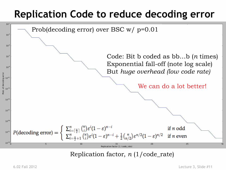
Replication Code to reduce decoding error
Replication factor, n (1/code_rate)
Prob(decoding error) over BSC w/ p=0.01
Code: Bit b coded as bb…b (n times) Exponential fall-off (note log scale) But huge overhead (low code rate)
We can do a lot better!
6.02 Fall 2012 Lecture 3, Slide #12
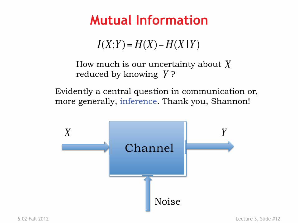
Mutual Information
Channel X Y
Noise
I(X;Y ) = H (X)−H (X |Y )
How much is our uncertainty about reduced by knowing ?
XY
Evidently a central question in communication or, more generally, inference. Thank you, Shannon!

6.02 Fall 2012 Lecture 3, Slide #13
Evaluating conditional entropy and mutual information
H (X |Y = yj ) = p(xii=1
m
∑ | yj )log21
p(xi | yj )
⎛
⎝⎜⎜
⎞
⎠⎟⎟
To compute conditional entropy:
H (X |Y ) = H (X |Y = yj )p(i=1
m
∑ yj )
because p(xi, yj ) = p(xi )p(yj | xi )
= p(yj )p(xi | y j )
I(X;Y ) = I(Y ;X)
H (X,Y ) = H (X)+H (Y | X)
= H (Y )+H (X |Y )so
mutual information is symmetric

6.02 Fall 2012 Lecture 3, Slide #14
e.g., Mutual information between input and output of
binary symmetric channel (BSC)
Channe l X ∈ {0,1} Y ∈ {0,1}
p
With probability the input binary digit gets flipped before being presented at the output.
p
I(X;Y ) = I(Y ;X) = H (Y )−H (Y | X)
=1−H (Y | X = 0)pX (0)−H (Y | X =1)pX (1)
=1− h(p)
Assume 0 and 1 are equally likely

6.02 Fall 2012 Lecture 3, Slide #15
Binary entropy function
Heads (or C=1) with probability Tails (or C=0) with probability
p
1− p
h(p)h(p)
p
H (C) = −p log2 p− (1− p)log2(1− p) = h(p)
1.0
0.5
1.0
0 0 0.5 1.0

6.02 Fall 2012 Lecture 3, Slide #16
So mutual information between input and output of the BSC with equally likely
inputs looks like this:
0.5 1.0
1.0 1− h(p)
p
For low-noise channel, significant reduction in uncertainty about the input after observing the output. For high-noise channel, little reduction.

6.02 Fall 2012 Lecture 3, Slide #17
Channel capacity
C =max I(X;Y ) =max H (X)−H (X |Y )}{
To characterize the channel, rather than the input and output, define where the maximization is over all possible distributions of . X
This is the most we can expect to reduce our uncertainty about through knowledge of , and so must be the most information we can expect to send through the channel on average, per use of the channel. Thank you, Shannon!
X Y
Channel X Y
Noise

6.02 Fall 2012 Lecture 3, Slide #18
C =1− h(p)�
0.5 1.0
1.0
Cha
nnel
cap
acity
p
e.g., capacity of the binary symmetric channel
C =max H (Y )−H (Y | X )}{Easiest to compute as , still over all possible probability distributions for . The second term doesn’t depend on this distribution, and the first term is maximized when 0 and 1 are equally likely at the input. So invoking our mutual information example earlier:
Channel X Y
p
X

6.02 Fall 2012 Lecture 3, Slide #19
What channel capacity tells us about how fast and how accurately we can communicate
…

6.02 Fall 2012 Lecture 3, Slide #20
The magic of asymptotically error-free transmission at any rate R <C
Shannon showed that one can theoretically transmit information (i.e., message bits) at an average rate per use of the channel, with arbitrarily low error. (He also showed the converse, that transmission at an average rate incurs an error probability that is lower-bounded by some positive number.)
R <C
R ≥C
The secret: Encode blocks of message bits into -bit codewords, so , with and very large.
k nR = k / n nk
Encoding blocks of message bits into -bit codewords to protect against channel errors is an example of channel coding
k n

6.02 Fall 2012 Lecture 3, Slide #21
Hamming Distance
The number of bit positions in which the corresponding bits of two encodings of the same length are different
The Hamming Distance (HD) between a valid binary codeword and the same codeword with e errors is e. The problem with no coding is that the two valid codewords ( 0 and 1 ) also have a Hamming distance of 1. So a single-bit error changes a valid codeword into another valid codeword… What is the Hamming Distance of the replication code?
1 0 heads tails
single-bit error
Th H i Di t (HD) b t
I wish he d increase his Hamming distance
����������������������� ��� ������������������������ ���������������

6.02 Fall 2012 Lecture 3, Slide #22
Idea: Embedding for Structural Separation Encode so that the codewords are far enough from each other Likely error patterns shouldn’t transform one codeword to another
11 00 0 1
01
10 single-bit error may cause 00 to be 10 (or 01)
110
000 0
1
100
010
111
001
101
011
Code: nodes chosen in hypercube + mapping of message bits to nodes
If we choose 2k out of 2n nodes, it means we can map all k-bit message strings in a space of n-bit codewords. The code rate is k/n.

6.02 Fall 2012 Lecture 3, Slide #23
Minimum Hamming Distance of Code vs. Detection & Correction Capabilities
If d is the minimum Hamming distance between codewords, we can detect all patterns of <= (d-1) bit errors
If d is the minimum Hamming distance between codewords, we can correct all patterns of
or fewer bit errors
d −12
⎢
⎣⎢⎥
⎦⎥

6.02 Fall 2012 Lecture 3, Slide #24
How to Construct Codes?
Want: 4-bit messages with single-error correction (min HD=3) How to produce a code, i.e., a set of codewords, with this property?

6.02 Fall 2012 Lecture 3, Slide #25
A Simple Code: Parity Check
• Add a parity bit to message of length k to make the total number of 1 bits even (aka even parity ).
• If the number of 1 s in the received word is odd, there there has been an error. 0 1 1 0 0 1 0 1 0 0 1 1 → original word with parity bit 0 1 1 0 0 0 0 1 0 0 1 1 → single-bit error (detected) 0 1 1 0 0 0 1 1 0 0 1 1 → 2-bit error (not detected)
• Minimum Hamming distance of parity check code is 2
– Can detect all single-bit errors
– In fact, can detect all odd number of errors – But cannot detect even number of errors
– And cannot correct any errors

6.02 Fall 2012 Lecture 3, Slide #26
Binary Arithmetic
• Computations with binary numbers in code construction will involve Boolean algebra, or algebra in “GF(2)” (Galois field of order 2), or modulo-2 algebra:
0+0=0, 1+0=0+1=1, 1+1=0
0*0=0*1=1*0 =0, 1*1=1

6.02 Fall 2012 Lecture 3, Slide #27
Linear Block Codes Block code: k message bits encoded to n code bits, i.e., each of 2k messages encoded into a unique n-bit combination via a linear transformation, using GF(2) operations: C=D.G C is an n-element row vector containing the codeword D is a k-element row vector containing the message G is the kxn generator matrix Each codeword bit is a specified linear combination of message bits. Key property: Sum of any two codewords is also a codeword � necessary and sufficient for code to be linear. (So the all-0 codeword has to be in any linear code --- why?) More on linear block codes in recitation & next lecture!!

6.02 Fall 2012 Lecture 3, Slide #28
Minimum HD of Linear Code
• (n,k) code has rate k/n
• Sometimes written as (n,k,d), where d is the minimum HD of the code.
• The “weight” of a code word is the number of 1’s in it.
• The minimum HD of a linear code is the minimum weight found in its nonzero codewords

6.02 Fall 2012 Lecture 3, Slide #29
Examples: What are n, k, d here?
{000, 111} {0000, 1100, 0011, 1111}
{1111, 0000, 0001}
{1111, 0000, 0010, 1100}
Not linear codes! Nc The HD of a
linear code is the number of “1”s in the non-zero codeword with the smallest # of “1”s
(3,1,3). Rate= 1/3. (4,2,2). Rate = ½.
(7,4,3) code. Rate = 4/7.
6.02 Fall 2012 Lecture 3, Slide #30
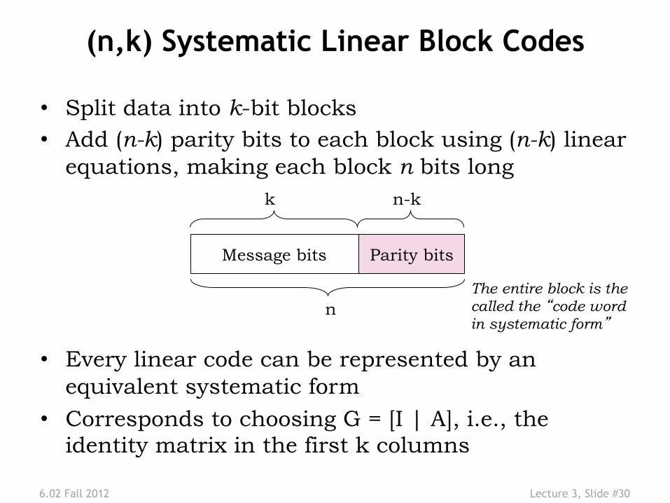
(n,k) Systematic Linear Block Codes
• Split data into k-bit blocks • Add (n-k) parity bits to each block using (n-k) linear
equations, making each block n bits long
• Every linear code can be represented by an equivalent systematic form
• Corresponds to choosing G = [I | A], i.e., the identity matrix in the first k columns
Message bits Parity bits
k
n The entire block is the called the code word in systematic form
n-k

MIT OpenCourseWarehttp://ocw.mit.edu
6.02 Introduction to EECS II: Digital Communication SystemsFall 2012
For information about citing these materials or our Terms of Use, visit: http://ocw.mit.edu/terms.
Recommended