16.1 Van Horne and Wachowicz, Fundamentals of Financial Management, 13th edition. © Pearson Education Limited 2009. Created by Gregory Kuhlemeyer.
Capítulo 16
Operating and Financial Leverage
Operating and Financial Leverage

16.2 Van Horne and Wachowicz, Fundamentals of Financial Management, 13th edition. © Pearson Education Limited 2009. Created by Gregory Kuhlemeyer.
1. Define operating and financial leverage and identify causes of both.
2. Calculate a firm’s operating break-even (quantity) point and break-even (sales) point .
3. Define, calculate, and interpret a firm's degree of operating, financial, and total leverage.
4. Understand EBIT-EPS break-even, or indifference, analysis, and construct and interpret an EBIT-EPS chart.
5. Define, discuss, and quantify “total firm risk” and its two components, “business risk” and “financial risk.”
6. Understand what is involved in determining the appropriate amount of financial leverage for a firm.
After Studying Chapter 16, you should be able to:

16.3 Van Horne and Wachowicz, Fundamentals of Financial Management, 13th edition. © Pearson Education Limited 2009. Created by Gregory Kuhlemeyer.
• Operating Leverage• Financial Leverage• Total Leverage• Cash-Flow Ability to Service Debt• Other Methods of Analysis• Combination of Methods
Operating and Financial Leverage

16.4 Van Horne and Wachowicz, Fundamentals of Financial Management, 13th edition. © Pearson Education Limited 2009. Created by Gregory Kuhlemeyer.
• One potential “effect” caused by the presence of operating leverage is that a change in the volume of sales results in a “more than proportional” change in operating profit (or loss).
Operating Leverage – The use of fixed operating costs by the firm.
Operating Leverage

16.5 Van Horne and Wachowicz, Fundamentals of Financial Management, 13th edition. © Pearson Education Limited 2009. Created by Gregory Kuhlemeyer.
Firm F Firm V Firm 2F
Sales $10 $11 $19.5Operating Costs
Fixed 7 2 14 Variable 2 7 3Operating Profit $ 1 $ 2 $
2.5
FC/total costs 0.78 0.22 0.82 FC/sales 0.70 0.18 0.72
(in thousands)
Impact of Operating Leverage on Profits

16.6 Van Horne and Wachowicz, Fundamentals of Financial Management, 13th edition. © Pearson Education Limited 2009. Created by Gregory Kuhlemeyer.
• Now, subject each firm to a 50% increase in sales for next year.
• Which firm do you think will be more “sensitive” to the change in sales (i.e., show the largest percentage changein operating profit, EBIT)?
[ ] Firm F; [ ] Firm V; [ ] Firm 2F.
Impact of Operating Leverage on Profits

16.7 Van Horne and Wachowicz, Fundamentals of Financial Management, 13th edition. © Pearson Education Limited 2009. Created by Gregory Kuhlemeyer.
Firm F Firm V Firm 2F
Sales $15 $16.5 $29.25Operating Costs Fixed 7 2 14 Variable 3 10.5 4.5Operating Profit $ 5 $ 4 $10.75
Percentage Change in EBIT* 400% 100% 330%
(in thousands)
* (EBITt - EBIT t-1) / EBIT t-1
Impact of Operating Leverage on Profits

16.8 Van Horne and Wachowicz, Fundamentals of Financial Management, 13th edition. © Pearson Education Limited 2009. Created by Gregory Kuhlemeyer.
• Firm F is the most “sensitive” firm – for it,a 50% increase in sales leads to a400% increase in EBIT.
• Our example reveals that it is a mistake to assume that the firm with the largest absolute
• or relative amount of fixed costs automatically shows the most dramatic effects of operating leverage.
• Later, we will come up with an easy way tospot the firm that is most sensitive to the presence of operating leverage.
Impact of Operating Leverage on Profits

16.9 Van Horne and Wachowicz, Fundamentals of Financial Management, 13th edition. © Pearson Education Limited 2009. Created by Gregory Kuhlemeyer.
• When studying operating leverage, “profits” refers to operating profits before taxes (i.e., EBIT) and excludes debt interest and dividend payments.
Break-Even Analysis – A technique for studying the relationship among fixed
costs, variable costs, sales volume, and profits. Also called cost/volume/profit
analysis (C/V/P) analysis.
Break-Even Analysis
16.10 Van Horne and Wachowicz, Fundamentals of Financial Management, 13th edition. © Pearson Education Limited 2009. Created by Gregory Kuhlemeyer.
QUANTITY PRODUCED AND SOLD
0 1,000 2,000 3,000 4,000 5,000 6,000 7,000
Total Revenues
Profits
Fixed Costs
Variable CostsLosses
RE
VE
NU
ES
AN
D C
OS
TS
($ t
ho
usa
nd
s)
175
250
100
50
Total Costs
Break-Even Chart

16.11 Van Horne and Wachowicz, Fundamentals of Financial Management, 13th edition. © Pearson Education Limited 2009. Created by Gregory Kuhlemeyer.
How to find the quantity break-even point:
EBIT = P(Q) – V(Q) – FC EBIT = Q(P – V) – FC
P = Price per unit V = Variable costs per unit FC = Fixed costs Q = Quantity (units)
produced and sold
Break-Even Point – The sales volume required so that total revenues and total costs are equal; may be in units or in sales dollars.
Break-Even (Quantity) Point

16.12 Van Horne and Wachowicz, Fundamentals of Financial Management, 13th edition. © Pearson Education Limited 2009. Created by Gregory Kuhlemeyer.
Breakeven occurs when EBIT = 0
Q (P – V) – FC = EBIT
QBE (P – V) – FC = 0
QBE (P – V) = FC
QBE = FC / (P – V)
a.k.a. Unit Contribution Margin
Break-Even (Quantity) Point

16.13 Van Horne and Wachowicz, Fundamentals of Financial Management, 13th edition. © Pearson Education Limited 2009. Created by Gregory Kuhlemeyer.
How to find the sales break-even point:
SBE = FC + (VCBE)
SBE = FC + (QBE )(V)
or
SBE*= FC / [1 – (VC / S) ]
* Refer to text for derivation of the formula
Break-Even (Sales) Point
16.14 Van Horne and Wachowicz, Fundamentals of Financial Management, 13th edition. © Pearson Education Limited 2009. Created by Gregory Kuhlemeyer.
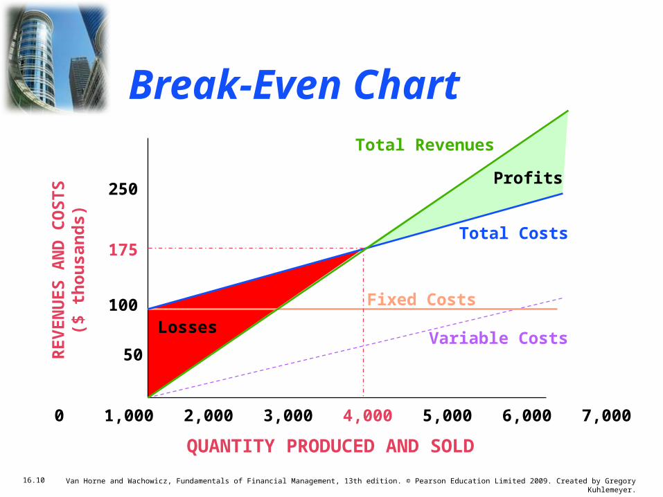
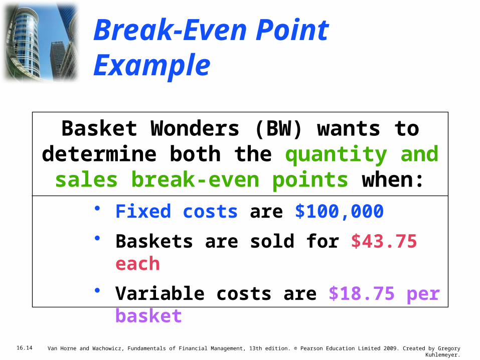
Basket Wonders (BW) wants to determine both the quantity and sales
break-even points when:• Fixed costs are $100,000
• Baskets are sold for $43.75 each
• Variable costs are $18.75 per basket
Break-Even Point Example

16.15 Van Horne and Wachowicz, Fundamentals of Financial Management, 13th edition. © Pearson Education Limited 2009. Created by Gregory Kuhlemeyer.
Breakeven occurs when:
QBE = FC / (P – V) QBE = $100,000 / ($43.75 – $18.75)QBE = 4,000 Units
SBE = (QBE )(V) + FCSBE = (4,000 )($18.75) + $100,000SBE = $175,000
Break-Even Point (s)

16.16 Van Horne and Wachowicz, Fundamentals of Financial Management, 13th edition. © Pearson Education Limited 2009. Created by Gregory Kuhlemeyer.
QUANTITY PRODUCED AND SOLD
0 1,000 2,000 3,000 4,000 5,000 6,000 7,000
Total Revenues
Profits
Fixed Costs
Variable CostsLosses
RE
VE
NU
ES
AN
D C
OS
TS
($ t
ho
usa
nd
s)
175
250
100
50
Total Costs
Break-Even Chart

16.17 Van Horne and Wachowicz, Fundamentals of Financial Management, 13th edition. © Pearson Education Limited 2009. Created by Gregory Kuhlemeyer.
DOL at Q units of output
(or sales)
Degree of Operating Leverage – The percentage change in a firm’s operating profit (EBIT) resulting from a 1 percent
change in output (sales).
=
Percentage change in operating profit (EBIT)
Percentage change in output (or sales)
Degree of Operating Leverage (DOL)

16.18 Van Horne and Wachowicz, Fundamentals of Financial Management, 13th edition. © Pearson Education Limited 2009. Created by Gregory Kuhlemeyer.
DOLQ units
Calculating the DOL for a single product or a single-product firm.
=Q (P – V)
Q (P – V) – FC
= Q
Q – QBE
Computing the DOL

16.19 Van Horne and Wachowicz, Fundamentals of Financial Management, 13th edition. © Pearson Education Limited 2009. Created by Gregory Kuhlemeyer.
DOLS dollars of
sales
Calculating the DOL for a multiproduct firm.
=S – VC
S – VC – FC
=EBIT + FC
EBIT
Computing the DOL

16.20 Van Horne and Wachowicz, Fundamentals of Financial Management, 13th edition. © Pearson Education Limited 2009. Created by Gregory Kuhlemeyer.
Lisa Miller wants to determine the degree of operating leverage at sales levels of 6,000 and 8,000 units. As we did earlier,
we will assume that:• Fixed costs are $100,000
• Baskets are sold for $43.75 each
• Variable costs are $18.75 per basket
Break-Even Point Example
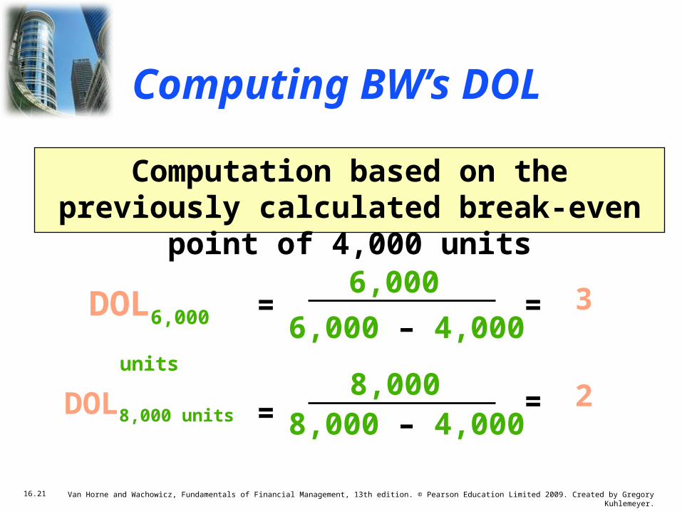
16.21 Van Horne and Wachowicz, Fundamentals of Financial Management, 13th edition. © Pearson Education Limited 2009. Created by Gregory Kuhlemeyer.
DOL6,000 units
Computation based on the previously calculated break-even point of 4,000 units
=6,000
6,000 – 4,000
=
= 3
DOL8,000 units
8,0008,000 – 4,000
= 2
Computing BW’s DOL

16.22 Van Horne and Wachowicz, Fundamentals of Financial Management, 13th edition. © Pearson Education Limited 2009. Created by Gregory Kuhlemeyer.
A 1% increase in sales above the 8,000 unit level increases EBIT by 2%
because of the existing operating leverage of the firm.
=DOL8,000 units
8,0008,000 – 4,000
= 2
Interpretation of the DOL

16.23 Van Horne and Wachowicz, Fundamentals of Financial Management, 13th edition. © Pearson Education Limited 2009. Created by Gregory Kuhlemeyer.
2,000 4,000 6,000 8,000
12345
QUANTITY PRODUCED AND SOLD
0–1–2–3
–4–5
DE
GR
EE
OF
OP
ER
AT
ING
LE
VE
RA
GE
(D
OL
)
QBE
Interpretation of the DOL

16.24 Van Horne and Wachowicz, Fundamentals of Financial Management, 13th edition. © Pearson Education Limited 2009. Created by Gregory Kuhlemeyer.
• DOL is a quantitative measure of the “sensitivity”of a firm’s operating profit to a change in the firm’s sales.
• The closer that a firm operates to its break-even point, the higher is the absolute value of its DOL.
• When comparing firms, the firm with the highest DOL is the firm that will be most “sensitive” to a change in sales.
Key Conclusions to be Drawn from the previous slide and our Discussion of DOL
Interpretation of the DOL

16.25 Van Horne and Wachowicz, Fundamentals of Financial Management, 13th edition. © Pearson Education Limited 2009. Created by Gregory Kuhlemeyer.
• DOL is only one component of business risk and becomes “active” only in the presence of sales and production cost variability.
• DOL magnifies the variability of operating profits and, hence, business risk.
Business Risk – The inherent uncertainty in the physical operations of the firm. Its impact is shown in the variability of the
firm’s operating income (EBIT).
DOL and Business Risk

16.26 Van Horne and Wachowicz, Fundamentals of Financial Management, 13th edition. © Pearson Education Limited 2009. Created by Gregory Kuhlemeyer.
Use the data in Slide 16–5 and the following formula for Firm F :
DOL = [(EBIT + FC)/EBIT]
=DOL$10,000 sales
1,000 + 7,0001,000
= 8.0
Application of DOL for Our Three Firm Example

16.27 Van Horne and Wachowicz, Fundamentals of Financial Management, 13th edition. © Pearson Education Limited 2009. Created by Gregory Kuhlemeyer.
Use the data in Slide 16–5 and the following formula for Firm V :
DOL = [(EBIT + FC)/EBIT]
=DOL$11,000 sales
2,000 + 2,0002,000
= 2.0
Application of DOL for Our Three Firm Example

16.28 Van Horne and Wachowicz, Fundamentals of Financial Management, 13th edition. © Pearson Education Limited 2009. Created by Gregory Kuhlemeyer.
Use the data in Slide 16–5 and the following formula for Firm 2F :
DOL = [(EBIT + FC)/EBIT]
=DOL$19,500 sales
2,500 + 14,0002,500
= 6.6
Application of DOL for Our Three-Firm Example

16.29 Van Horne and Wachowicz, Fundamentals of Financial Management, 13th edition. © Pearson Education Limited 2009. Created by Gregory Kuhlemeyer.
The ranked results indicate that the firm most sensitive to the presence of operating leverage
is Firm F.
Firm F DOL = 8.0Firm V DOL = 6.6Firm 2F DOL = 2.0
Firm F will expect a 400% increase in profit from a 50% increase in sales (see Slide 16–7 results).
Application of DOL for Our Three-Firm Example

16.30 Van Horne and Wachowicz, Fundamentals of Financial Management, 13th edition. © Pearson Education Limited 2009. Created by Gregory Kuhlemeyer.
• Financial leverage is acquired by choice.
• Used as a means of increasing the return to common shareholders.
Financial Leverage – The use of fixed financing costs by the firm. The British expression is gearing.
Financial Leverage
16.31 Van Horne and Wachowicz, Fundamentals of Financial Management, 13th edition. © Pearson Education Limited 2009. Created by Gregory Kuhlemeyer.
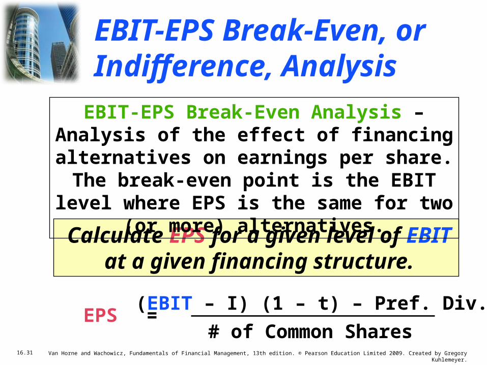
Calculate EPS for a given level of EBIT at a given financing structure.
EBIT-EPS Break-Even Analysis – Analysis of the effect of financing alternatives on
earnings per share. The break-even point is the EBIT level where EPS is the same for
two (or more) alternatives.
(EBIT – I) (1 – t) – Pref. Div.
# of Common SharesEPS =
EBIT-EPS Break-Even, or Indifference, Analysis

16.32 Van Horne and Wachowicz, Fundamentals of Financial Management, 13th edition. © Pearson Education Limited 2009. Created by Gregory Kuhlemeyer.
• Current common equity shares = 50,000
• $1 million in new financing of either:• All C.S. sold at $20/share (50,000 shares)• All debt with a coupon rate of 10%• All P.S. with a dividend rate of 9%
• Expected EBIT = $500,000• Income tax rate is 30%
Basket Wonders has $2 million in LT financing (100% common stock equity).
EBIT-EPS Chart

16.33 Van Horne and Wachowicz, Fundamentals of Financial Management, 13th edition. © Pearson Education Limited 2009. Created by Gregory Kuhlemeyer.
EBIT $500,000 $150,000*
Interest 0 0
EBT $500,000 $150,000
Taxes (30% x EBT) 150,000 45,000
EAT $350,000 $105,000
Preferred Dividends 0 0
EACS $350,000 $105,000
# of Shares 100,000 100,000
EPS $3.50 $1.05
Common Stock Equity Alternative
* A second analysis using $150,000 EBIT rather than the expected EBIT.
EBIT-EPS Calculation with New Equity Financing

16.34 Van Horne and Wachowicz, Fundamentals of Financial Management, 13th edition. © Pearson Education Limited 2009. Created by Gregory Kuhlemeyer.
0 100 200 300 400 500 600 700
EBIT ($ thousands)
Ear
nin
gs
per
Sh
are
($)
0
1
2
3
4
5
6
Common
EBIT-EPS Chart
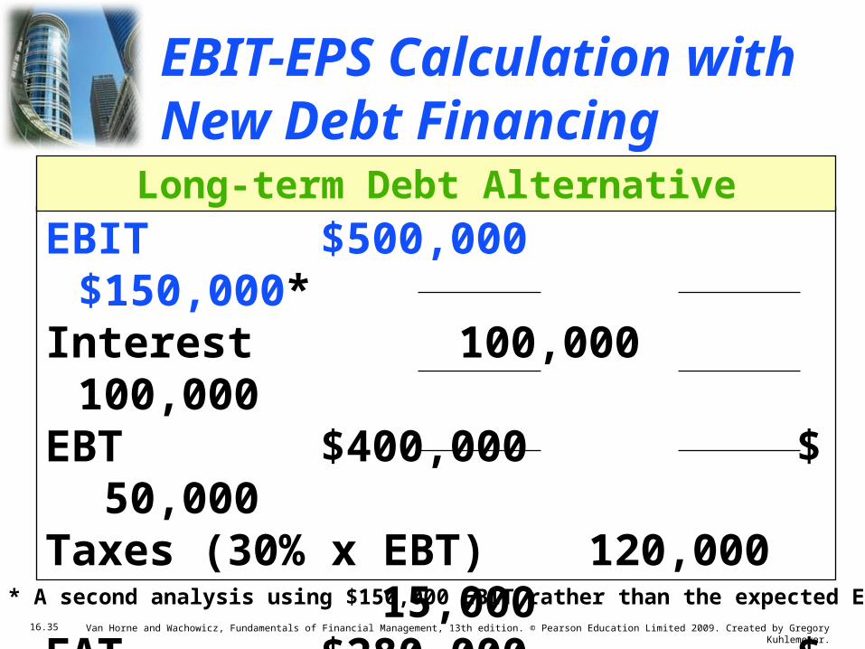
16.35 Van Horne and Wachowicz, Fundamentals of Financial Management, 13th edition. © Pearson Education Limited 2009. Created by Gregory Kuhlemeyer.
EBIT $500,000 $150,000*
Interest 100,000 100,000
EBT $400,000 $ 50,000
Taxes (30% x EBT) 120,000 15,000
EAT $280,000 $ 35,000
Preferred Dividends 0 0
EACS $280,000 $ 35,000
# of Shares 50,000 50,000
EPS $5.60 $0.70
Long-term Debt Alternative
* A second analysis using $150,000 EBIT rather than the expected EBIT.
EBIT-EPS Calculation with New Debt Financing

16.36 Van Horne and Wachowicz, Fundamentals of Financial Management, 13th edition. © Pearson Education Limited 2009. Created by Gregory Kuhlemeyer.
0 100 200 300 400 500 600 700
EBIT ($ thousands)
Ear
nin
gs
per
Sh
are
($)
0
1
2
3
4
5
6
Common
Debt
Indifference pointbetween debt and
common stockfinancing
EBIT-EPS Chart

16.37 Van Horne and Wachowicz, Fundamentals of Financial Management, 13th edition. © Pearson Education Limited 2009. Created by Gregory Kuhlemeyer.
EBIT $500,000 $150,000*
Interest 0 0
EBT $500,000 $150,000
Taxes (30% x EBT) 150,000 45,000
EAT $350,000 $105,000
Preferred Dividends 90,000 90,000
EACS $260,000 $ 15,000
# of Shares 50,000 50,000
EPS $5.20 $0.30
Preferred Stock Alternative
* A second analysis using $150,000 EBIT rather than the expected EBIT.
EBIT-EPS Calculation with New Preferred Financing

16.38 Van Horne and Wachowicz, Fundamentals of Financial Management, 13th edition. © Pearson Education Limited 2009. Created by Gregory Kuhlemeyer.
0 100 200 300 400 500 600 700
EBIT ($ thousands)
Ear
nin
gs
per
Sh
are
($)
0
1
2
3
4
5
6
Common
Debt
Indifference pointbetween preferred stock and common
stock financing
Preferred
EBIT-EPS Chart

16.39 Van Horne and Wachowicz, Fundamentals of Financial Management, 13th edition. © Pearson Education Limited 2009. Created by Gregory Kuhlemeyer.
0 100 200 300 400 500 600 700
EBIT ($ thousands)
Ear
nin
gs
per
Sh
are
($)
0
1
2
3
4
5
6
Common
Debt
Lower risk. Only a smallprobability that EPS willbe less if the debtalternative is chosen.
Pro
bab
ility of O
ccurren
ce(fo
r the p
rob
ability d
istribu
tion
)What About Risk?

16.40 Van Horne and Wachowicz, Fundamentals of Financial Management, 13th edition. © Pearson Education Limited 2009. Created by Gregory Kuhlemeyer.
0 100 200 300 400 500 600 700
EBIT ($ thousands)
Ear
nin
gs
per
Sh
are
($)
0
1
2
3
4
5
6
Common
Debt
Higher risk. A much largerprobability that EPS willbe less if the debtalternative is chosen.
Pro
bab
ility of O
ccurren
ce(fo
r the p
rob
ability d
istribu
tion
)What About Risk?

16.41 Van Horne and Wachowicz, Fundamentals of Financial Management, 13th edition. © Pearson Education Limited 2009. Created by Gregory Kuhlemeyer.
DFL at EBIT of
X dollars
Degree of Financial Leverage – The percentage change in a firm’s earnings
per share (EPS) resulting from a 1 percent change in operating profit.
=
Percentage change in earnings per share (EPS)
Percentage change in operating profit (EBIT)
Degree of Financial Leverage (DFL)

16.42 Van Horne and Wachowicz, Fundamentals of Financial Management, 13th edition. © Pearson Education Limited 2009. Created by Gregory Kuhlemeyer.
DFL EBIT of $X
Calculating the DFL
=EBIT
EBIT – I – [ PD / (1 – t) ]
EBIT = Earnings before interest and taxesI = InterestPD = Preferred dividendst = Corporate tax rate
Computing the DFL

16.43 Van Horne and Wachowicz, Fundamentals of Financial Management, 13th edition. © Pearson Education Limited 2009. Created by Gregory Kuhlemeyer.
DFL $500,000
Calculating the DFL for NEW equity* alternative
=$500,000
$500,000 – 0 – [0 / (1 – 0)]
* The calculation is based on the expected EBIT
= 1.00
What is the DFL for Each of the Financing Choices?

16.44 Van Horne and Wachowicz, Fundamentals of Financial Management, 13th edition. © Pearson Education Limited 2009. Created by Gregory Kuhlemeyer.
DFL $500,000
Calculating the DFL for NEW debt * alternative
=$500,000
{ $500,000 – 100,000 – [0 / (1 – 0)] }
* The calculation is based on the expected EBIT
= $500,000 / $400,000
1.25=
What is the DFL for Each of the Financing Choices?

16.45 Van Horne and Wachowicz, Fundamentals of Financial Management, 13th edition. © Pearson Education Limited 2009. Created by Gregory Kuhlemeyer.
DFL $500,000
Calculating the DFL for NEW preferred * alternative
=$500,000
{ $500,000 – 0 – [90,000 / (1 – 0.30)] }
* The calculation is based on the expected EBIT
= $500,000 / $371,429
1.35=
What is the DFL for Each of the Financing Choices?
16.46 Van Horne and Wachowicz, Fundamentals of Financial Management, 13th edition. © Pearson Education Limited 2009. Created by Gregory Kuhlemeyer.
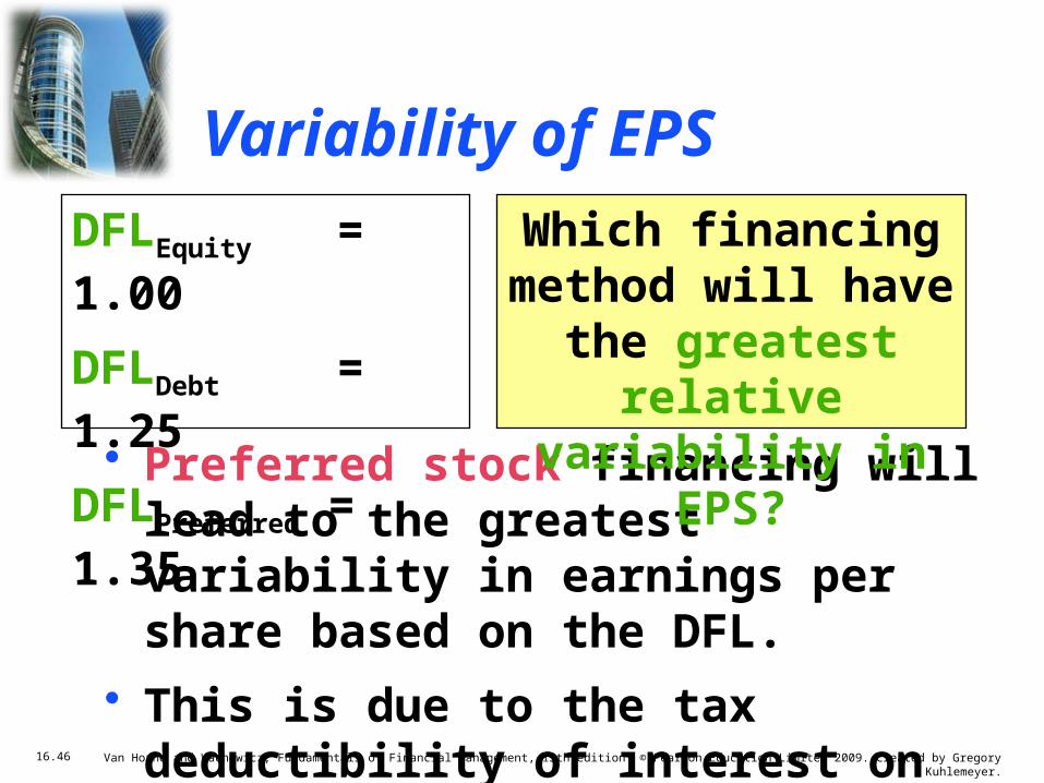
• Preferred stock financing will lead to the greatest variability in earnings per share based on the DFL.
• This is due to the tax deductibility of interest on debt financing.
DFLEquity = 1.00
DFLDebt = 1.25
DFLPreferred = 1.35
Which financing method will have
the greatest relative variability in EPS?
Variability of EPS

16.47 Van Horne and Wachowicz, Fundamentals of Financial Management, 13th edition. © Pearson Education Limited 2009. Created by Gregory Kuhlemeyer.
• Debt increases the probability of cash insolvency over an all-equity-financed firm. For example, our example firm must have EBIT of at least $100,000 to cover the interest payment.
• Debt also increased the variability in EPS as the DFL increased from 1.00 to 1.25.
Financial Risk – The added variability in earnings per share (EPS) – plus the risk of
possible insolvency – that is induced by the use of financial leverage.
Financial Risk

16.48 Van Horne and Wachowicz, Fundamentals of Financial Management, 13th edition. © Pearson Education Limited 2009. Created by Gregory Kuhlemeyer.
• CVEPS is a measure of relative total firm risk
• CVEBIT is a measure of relative business risk
• The difference, CVEPS – CVEBIT, is a measure of relative financial risk
Total Firm Risk – The variability in earnings per share (EPS). It is the sum of business plus
financial risk.
Total firm risk = business risk + financial risk
Total Firm Risk
16.49 Van Horne and Wachowicz, Fundamentals of Financial Management, 13th edition. © Pearson Education Limited 2009. Created by Gregory Kuhlemeyer.
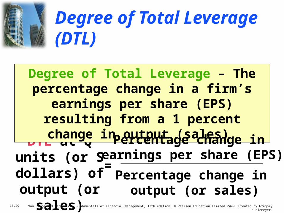
DTL at Q units (or S dollars) of output (or
sales)
Degree of Total Leverage – The percentage change in a firm’s earnings
per share (EPS) resulting from a 1 percent change in output (sales).
=
Percentage change in earnings per share (EPS)
Percentage change in output (or sales)
Degree of Total Leverage (DTL)

16.50 Van Horne and Wachowicz, Fundamentals of Financial Management, 13th edition. © Pearson Education Limited 2009. Created by Gregory Kuhlemeyer.
DTL S dollars
of sales
DTL Q units (or S dollars) = ( DOL Q units (or S dollars) ) x ( DFL EBIT of X dollars )
=EBIT + FC
EBIT – I – [ PD / (1 – t) ]
DTL Q unitsQ (P – V)
Q (P – V) – FC – I – [ PD / (1 – t) ]=
Computing the DTL

16.51 Van Horne and Wachowicz, Fundamentals of Financial Management, 13th edition. © Pearson Education Limited 2009. Created by Gregory Kuhlemeyer.
Lisa Miller wants to determine the Degree of Total Leverage at
EBIT=$500,000. As we did earlier, we will assume that:
• Fixed costs are $100,000
• Baskets are sold for $43.75 each
• Variable costs are $18.75 per basket
DTL Example

16.52 Van Horne and Wachowicz, Fundamentals of Financial Management, 13th edition. © Pearson Education Limited 2009. Created by Gregory Kuhlemeyer.
DTL S dollars
of sales
=$500,000 + $100,000
$500,000 – 0 – [ 0 / (1 – 0.3) ]
DTLS dollars = (DOL S dollars) x (DFLEBIT of $S )
DTLS dollars = (1.2 ) x ( 1.0* ) = 1.20
= 1.20*Note: No financial leverage.
Computing the DTL for All-Equity Financing
16.53 Van Horne and Wachowicz, Fundamentals of Financial Management, 13th edition. © Pearson Education Limited 2009. Created by Gregory Kuhlemeyer.
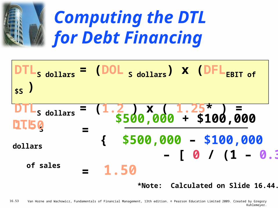
DTL S dollars
of sales
=$500,000 + $100,000
{ $500,000 – $100,000 – [ 0 / (1 – 0.3) ] }
DTLS dollars = (DOL S dollars) x (DFLEBIT of $S )
DTLS dollars = (1.2 ) x ( 1.25* ) = 1.50
= 1.50*Note: Calculated on Slide 16.44.
Computing the DTL for Debt Financing

16.54 Van Horne and Wachowicz, Fundamentals of Financial Management, 13th edition. © Pearson Education Limited 2009. Created by Gregory Kuhlemeyer.
Compare the expected EPS to the DTL for the common stock equity financing
approach to the debt financing approach.
Financing E(EPS) DTL
Equity $3.50 1.20 Debt $5.60 1.50Greater expected return (higher EPS) comes at the
expense of greater potential risk (higher DTL)!
Risk versus Return

16.55 Van Horne and Wachowicz, Fundamentals of Financial Management, 13th edition. © Pearson Education Limited 2009. Created by Gregory Kuhlemeyer.
• Firms must first analyze their expected future cash flows.
• The greater and more stable the expected future cash flows, the greater the debt capacity.
• Fixed charges include: debt principal and interest payments, lease payments, and preferred stock dividends.
Debt Capacity – The maximum amount of debt (and other fixed-charge financing) that a firm
can adequately service.
What is an Appropriate Amount of Financial Leverage?
16.56 Van Horne and Wachowicz, Fundamentals of Financial Management, 13th edition. © Pearson Education Limited 2009. Created by Gregory Kuhlemeyer.
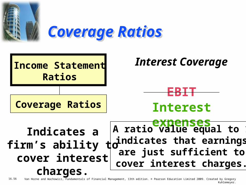
Interest Coverage
EBITInterest expenses
Interest Coverage
EBITInterest expenses
Indicates a firm’s ability to cover
interest charges.
Income StatementRatios
Coverage Ratios
A ratio value equal to 1indicates that earnings
are just sufficient tocover interest charges.
Coverage RatiosCoverage Ratios
16.57 Van Horne and Wachowicz, Fundamentals of Financial Management, 13th edition. © Pearson Education Limited 2009. Created by Gregory Kuhlemeyer.
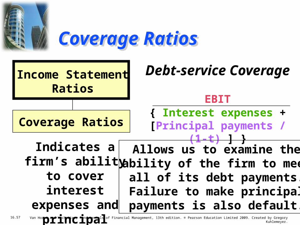
Debt-service Coverage
EBIT{ Interest expenses +
[Principal payments / (1-t) ] }
Debt-service Coverage
EBIT{ Interest expenses +
[Principal payments / (1-t) ] }
Indicates a firm’s ability to cover
interest expenses and principal
payments.
Income StatementRatios
Coverage Ratios
Allows us to examine theability of the firm to meetall of its debt payments.Failure to make principalpayments is also default.
Coverage RatiosCoverage Ratios
16.58 Van Horne and Wachowicz, Fundamentals of Financial Management, 13th edition. © Pearson Education Limited 2009. Created by Gregory Kuhlemeyer.
Make an examination of the coverage ratios for Basket Wonders when
EBIT=$500,000. Compare the equity and the debt financing alternatives.
Assume that:• Interest expenses remain at $100,000
• Principal payments of $100,000 are made yearly for 10 years
Coverage Example

16.59 Van Horne and Wachowicz, Fundamentals of Financial Management, 13th edition. © Pearson Education Limited 2009. Created by Gregory Kuhlemeyer.
Compare the interest coverage and debt burden ratios for equity and debt financing.
Interest Debt-service Financing Coverage Coverage
Equity Infinite Infinite Debt 5.00 2.50The firm actually has greater risk than the interest
coverage ratio initially suggests.
Coverage Example

16.60 Van Horne and Wachowicz, Fundamentals of Financial Management, 13th edition. © Pearson Education Limited 2009. Created by Gregory Kuhlemeyer.
-250 0 250 500 750 1,000 1,250
EBIT ($ thousands)
Firm B has a much smaller probability
of failing to meet its obligations than Firm A.
Firm B
Firm A
Debt-service burden= $200,000
PR
OB
AB
ILIT
Y O
F O
CC
UR
RE
NC
ECoverage Example

16.61 Van Horne and Wachowicz, Fundamentals of Financial Management, 13th edition. © Pearson Education Limited 2009. Created by Gregory Kuhlemeyer.
• A single ratio value cannot be interpreted identically for all firms as some firms have greater debt capacity.
• Annual financial lease payments should be added to both the numerator and denominator of the debt-service coverage ratio as financial leases are similar to debt.
• A single ratio value cannot be interpreted identically for all firms as some firms have greater debt capacity.
• Annual financial lease payments should be added to both the numerator and denominator of the debt-service coverage ratio as financial leases are similar to debt.
• The debt-service coverage ratio accounts for required annual principal payments.
• The debt-service coverage ratio accounts for required annual principal payments.
Summary of the Coverage Ratio DiscussionSummary of the Coverage Ratio Discussion

16.62 Van Horne and Wachowicz, Fundamentals of Financial Management, 13th edition. © Pearson Education Limited 2009. Created by Gregory Kuhlemeyer.
• Often, firms are compared to peer institutions in the same industry.
• Large deviations from norms must be justified.
• For example, an industry’s median debt-to-net-worth ratio might be used as a benchmark for financial leverage comparisons.
Capital Structure – The mix (or proportion) of a firm’s permanent long-term financing
represented by debt, preferred stock, and common stock equity.
Other Methods of Analysis

16.63 Van Horne and Wachowicz, Fundamentals of Financial Management, 13th edition. © Pearson Education Limited 2009. Created by Gregory Kuhlemeyer.
• Firms may gain insight into the financial markets’ evaluation of their firm by talking with:
• Investment bankers• Institutional investors• Investment analysts• Lenders
Surveying Investment Analysts and Lenders
Other Methods of Analysis

16.64 Van Horne and Wachowicz, Fundamentals of Financial Management, 13th edition. © Pearson Education Limited 2009. Created by Gregory Kuhlemeyer.
• Firms must consider the impact of any financing decision on the firm’s security rating(s).
Security Ratings
Other Methods of Analysis
Recommended