1ENTS689L: Packet Processing and SwitchingBuffer-less Switch Fabric Architectures
Buffer-less Switch Fabric Architectures
Vahid Tabatabaee
Fall 2006

2ENTS689L: Packet Processing and SwitchingBuffer-less Switch Fabric Architectures
References
Light Reading Report on Switch Fabrics, available online at: http://www.lightreading.com/document.asp?doc_id=25989
Title: Network Processors Architectures, Protocols, and PlatformsAuthor: Panos C. LekkasPublisher: McGraw-Hill
I. Elhanany, D. Chiou, V. Tabatabaee, R. Noro, A. Poursepanj, “The Network Processing Forum Switch Fabric Benchmark Specifications: An Overview”, IEEE Network Magazine, March/April 2005.

3ENTS689L: Packet Processing and SwitchingBuffer-less Switch Fabric Architectures
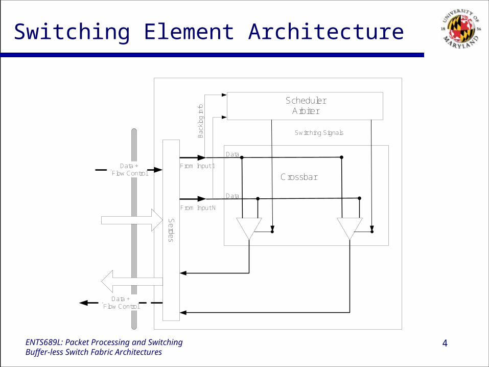
Buffer-less Switching Element
There is no major buffering in the switching element. The only buffering is for alignment of the cells. Incoming cells after alignment are simultaneously
switched to the output ports The performance of the switch is very much dependent
on the scheduling algorithm.
4ENTS689L: Packet Processing and SwitchingBuffer-less Switch Fabric Architectures
Switching Element Architecture
Se
rde
s
Data +Flow Control
Data +Flow Control
SchedulerArbiter
CrossbarFrom Input 1
From Input N
Data
DataB
ackl
og in
fo
Switching Signals

5ENTS689L: Packet Processing and SwitchingBuffer-less Switch Fabric Architectures
Data flow in the switching element
Cells are continuously sent from line card to the switch card and from the switch card to the line card.
Transmitted cells may not have valid data. Switch scheduler decides about connection between input and
output port and then send the corresponding command to the line interface chip.
The line interface chip send one cell destined to the corresponding output port to the switch.
The switching element needs to have some information about the backlogged cells in the input ports.
The line card interface needs to know about its designated output port in the next time slot.
The last two bullets info. are sent through the cell header from the line interface to the switch and from the switch to the line interface respectively.
6ENTS689L: Packet Processing and SwitchingBuffer-less Switch Fabric Architectures
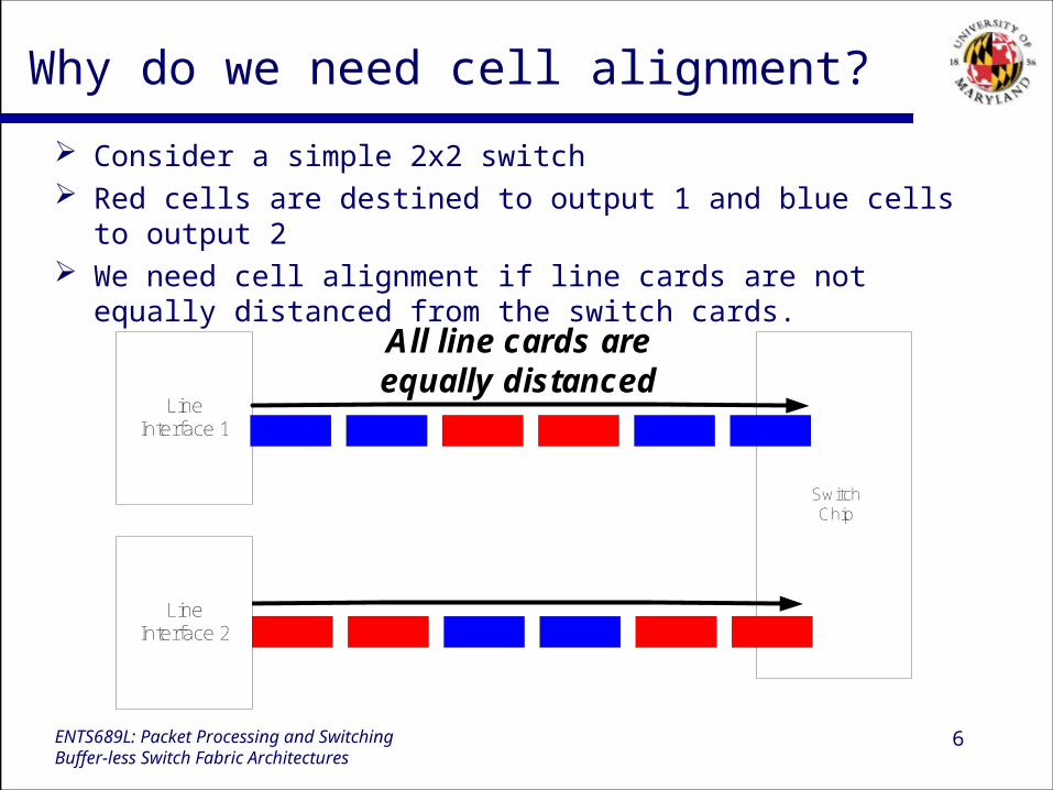
Why do we need cell alignment?
Consider a simple 2x2 switch Red cells are destined to output 1 and blue cells to output 2 We need cell alignment if line cards are not equally distanced from
the switch cards.
LineInterface 1
SwitchChip
All line cards areequally distanced
LineInterface 2

7ENTS689L: Packet Processing and SwitchingBuffer-less Switch Fabric Architectures
Why do we need cell alignment?
If the cells are not aligned we may end up with switching cells to the wrong destination or contention between cells going to the same destination
LineInterface 1
SwitchChip
All line cards are notequally distanced
LineInterface 2
8ENTS689L: Packet Processing and SwitchingBuffer-less Switch Fabric Architectures
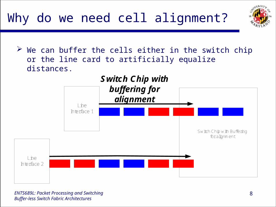
Why do we need cell alignment?
We can buffer the cells either in the switch chip or the line card to artificially equalize distances.
LineInterface 1
Switch Chip with Bufferingfor alignment
Switch Chip withbuffering for
alignment
LineInterface 2
9ENTS689L: Packet Processing and SwitchingBuffer-less Switch Fabric Architectures
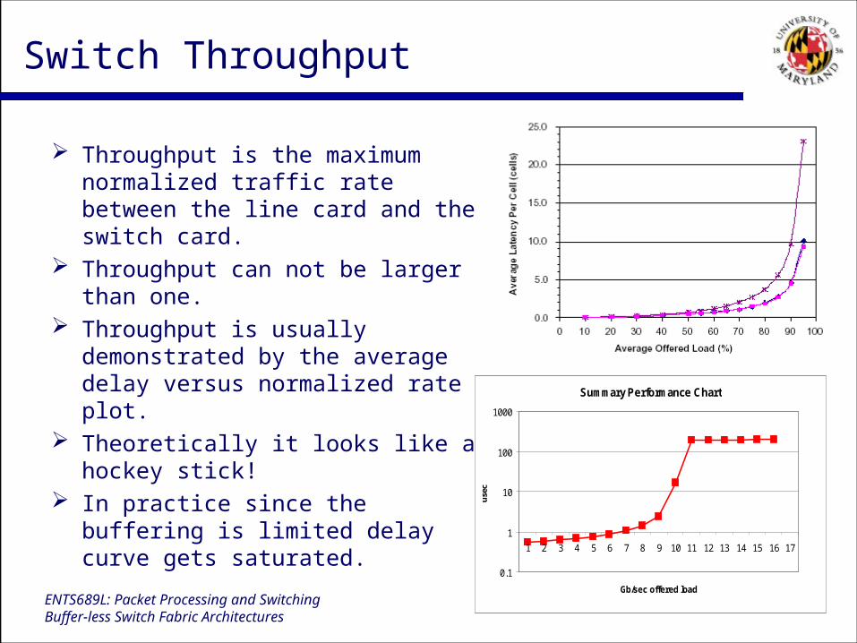
Switch Throughput
Throughput is the maximum normalized traffic rate between the line card and the switch card.
Throughput can not be larger than one.
Throughput is usually demonstrated by the average delay versus normalized rate plot.
Theoretically it looks like a hockey stick!
In practice since the buffering is limited delay curve gets saturated.
Summary Performance Chart
0.1
1
10
100
1000
1 2 3 4 5 6 7 8 9 10 11 12 13 14 15 16 17
Gb/sec offered load
use
c
10ENTS689L: Packet Processing and SwitchingBuffer-less Switch Fabric Architectures
What causes throughput limitation
If there is no contention between the input and output ports throughput can go up to 100%.
Due to contention some ports can remain idle even though they have cell to send/receive.
The scheduling algorithm decides about input-output connection and resolves contentions.
Therefore scheduling algorithm determines throughput of a switch.
11ENTS689L: Packet Processing and SwitchingBuffer-less Switch Fabric Architectures
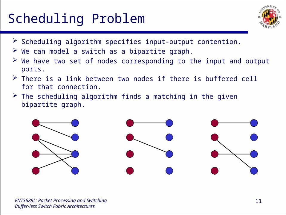
Scheduling Problem
Scheduling algorithm specifies input-output contention. We can model a switch as a bipartite graph. We have two set of nodes corresponding to the input and output ports. There is a link between two nodes if there is buffered cell for that
connection. The scheduling algorithm finds a matching in the given bipartite graph.
12ENTS689L: Packet Processing and SwitchingBuffer-less Switch Fabric Architectures
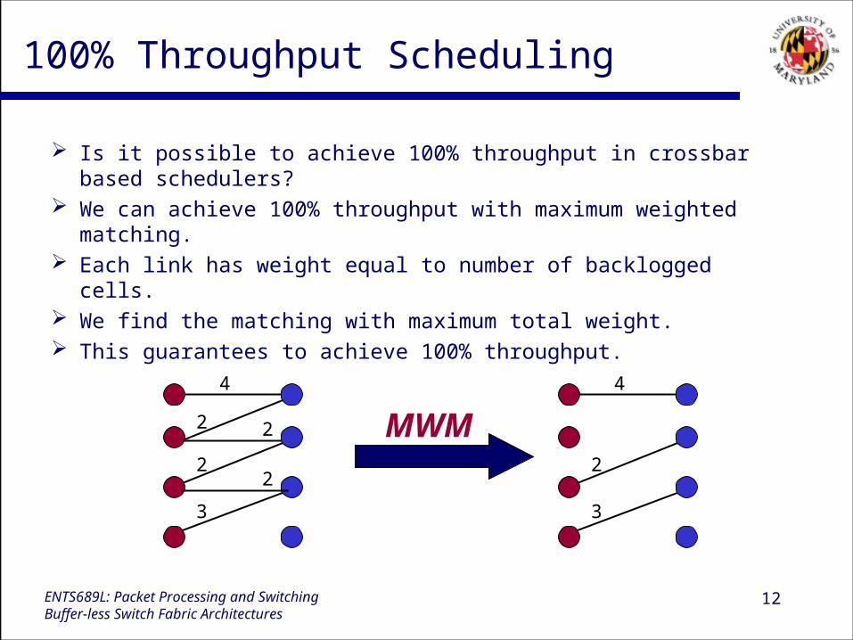
100% Throughput Scheduling
Is it possible to achieve 100% throughput in crossbar based schedulers?
We can achieve 100% throughput with maximum weighted matching.
Each link has weight equal to number of backlogged cells. We find the matching with maximum total weight. This guarantees to achieve 100% throughput.
4
2 2
22
3
4
2
3
MWM

13ENTS689L: Packet Processing and SwitchingBuffer-less Switch Fabric Architectures
Alternative 100% Throughput Algorithms
Alternative algorithms to achieve 100% throughput. Maximum Weighted Matching (MWM): Maximizes total weight of
links; O(N3) complexity. Longest Port First (LPF): Maximizes total weight of nodes; O(N3)
complexity. Maximum Node Containing Matching (MNCM): Includes all nodes
that their weight are greater than (1-1/N) of maximum node weight; O(N2.5) complexity.
4
2 2
22
3
4
2
2
MWM LPF MNCM
14ENTS689L: Packet Processing and SwitchingBuffer-less Switch Fabric Architectures
Practical Approaches
These algorithms are not amenable to hardware implementation
We use simple algorithms that are simple and can be implemented in hardware.
To compensate for their low performance we make the switch works faster than the line-card (speedup).
It is proved that any maximal size matching with 2X speedup can achieve 100% throughput.
A matching is maximal if it is not possible to add anymore link to the matching.
15ENTS689L: Packet Processing and SwitchingBuffer-less Switch Fabric Architectures
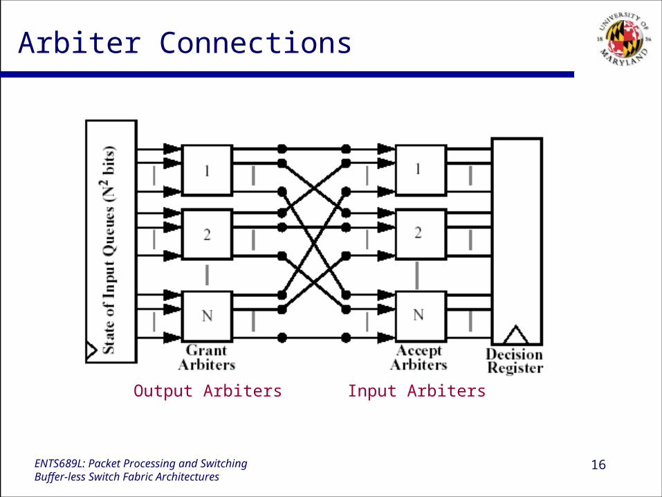
iSLIP Scheduling Algorithm
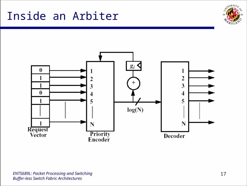
There is an arbiter associated with every input and output node. Every arbiter receives up to N active signals and select one of
them using a round-robin scheduler. Every output arbiter receives request signal from all inputs that
have a backlogged cell. It grants the first request after the previously ACCEPTED grant. Input arbiters accept the first grant after the previously accepted
grant. Every arbiter has a pointer that points to the previously accepted
port.
16ENTS689L: Packet Processing and SwitchingBuffer-less Switch Fabric Architectures
Arbiter Connections
Output Arbiters Input Arbiters
17ENTS689L: Packet Processing and SwitchingBuffer-less Switch Fabric Architectures
Inside an Arbiter
18ENTS689L: Packet Processing and SwitchingBuffer-less Switch Fabric Architectures
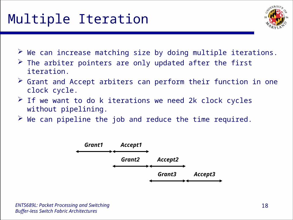
Multiple Iteration
We can increase matching size by doing multiple iterations. The arbiter pointers are only updated after the first iteration. Grant and Accept arbiters can perform their function in one clock
cycle. If we want to do k iterations we need 2k clock cycles without
pipelining. We can pipeline the job and reduce the time required.
Grant1 Accept1
Grant2 Accept2
Grant3 Accept3
19ENTS689L: Packet Processing and SwitchingBuffer-less Switch Fabric Architectures
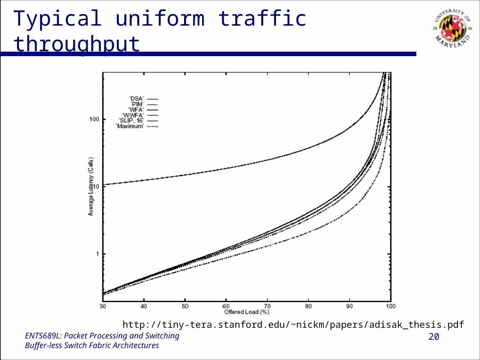
iSLIP Throughput and arrival process
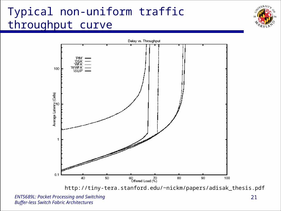
Good performance for uniform traffic. Degraded performance for non-uniform traffic. In general performance of a switch depends on the characteristics of the
input data. In a switch there are three important characteristics: Arrival Pattern:
Uniform: Usually modeled as Bernoulli i.i.d arrivals. At each time slot there is a probability p of new arrival.
Non-uniform: Usually modeled with a two-state Markov Chain If we are in ON state we keep generating packets. If we are in OFF state no packet is generated.
Packet length: Number of bytes in generated packets. Load distribution: Destination of packets generated at each input
Uniform: Packets are divide among destinations with equal probability Non-Uniform: Some destinations are more probable (Hot Spots).
20ENTS689L: Packet Processing and SwitchingBuffer-less Switch Fabric Architectures
Typical uniform traffic throughput
http://tiny-tera.stanford.edu/~nickm/papers/adisak_thesis.pdf
21ENTS689L: Packet Processing and SwitchingBuffer-less Switch Fabric Architectures
Typical non-uniform traffic throughput curve
http://tiny-tera.stanford.edu/~nickm/papers/adisak_thesis.pdf
22ENTS689L: Packet Processing and SwitchingBuffer-less Switch Fabric Architectures
Benchmarking & Comparison of Switch Fabrics
How do we have to compare switch fabrics First we have to compare general design parameters. Second we have to compare performance of the fabrics.
23ENTS689L: Packet Processing and SwitchingBuffer-less Switch Fabric Architectures
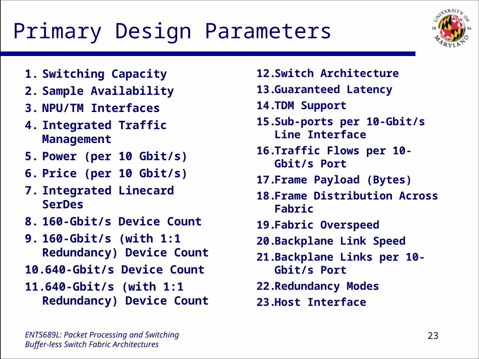
Primary Design Parameters
1. Switching Capacity
2. Sample Availability
3. NPU/TM Interfaces
4. Integrated Traffic Management
5. Power (per 10 Gbit/s)
6. Price (per 10 Gbit/s)
7. Integrated Linecard SerDes
8. 160-Gbit/s Device Count
9. 160-Gbit/s (with 1:1 Redundancy) Device Count
10.640-Gbit/s Device Count
11.640-Gbit/s (with 1:1 Redundancy) Device Count
12. Switch Architecture
13. Guaranteed Latency
14. TDM Support
15. Sub-ports per 10-Gbit/s Line Interface
16. Traffic Flows per 10-Gbit/s Port
17. Frame Payload (Bytes)
18. Frame Distribution Across Fabric
19. Fabric Overspeed
20. Backplane Link Speed
21. Backplane Links per 10-Gbit/s Port
22. Redundancy Modes
23. Host Interface
24ENTS689L: Packet Processing and SwitchingBuffer-less Switch Fabric Architectures
Performance Benchmarking
Traffic Modeling
Performance Metrics
Benchmark Suites
25ENTS689L: Packet Processing and SwitchingBuffer-less Switch Fabric Architectures
Traffic Modeling
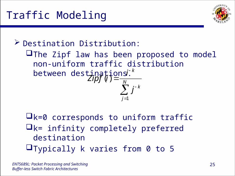
Destination Distribution:The Zipf law has been proposed to model non-
uniform traffic distribution between destinations.
k=0 corresponds to uniform traffick= infinity completely preferred destinationTypically k varies from 0 to 5
N
j
k
k
j
iiZipf
1
)(

26ENTS689L: Packet Processing and SwitchingBuffer-less Switch Fabric Architectures
Traffic Modeling
Packet arrival process: Bernoulli i.i.d. arrivals ON/OFF model ON/OFF model with non-delimited burst streams ON/OFF model with minimum burst size.
Mulitcast Multiplicity factor: Realistically should not exceed 10 with an
average value of 2-4. Distribution of the detinations
QoS Distribution of the traffic among a number of classes
27ENTS689L: Packet Processing and SwitchingBuffer-less Switch Fabric Architectures
Performance Metrics
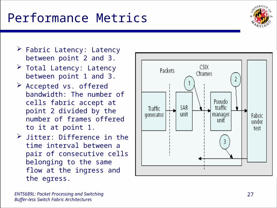
Fabric Latency: Latency between point 2 and 3.
Total Latency: Latency between point 1 and 3.
Accepted vs. offered bandwidth: The number of cells fabric accept at point 2 divided by the number of frames offered to it at point 1.
Jitter: Difference in the time interval between a pair of consecutive cells belonging to the same flow at the ingress and the egress.

28ENTS689L: Packet Processing and SwitchingBuffer-less Switch Fabric Architectures
Benchmark Suites
Hardware Benchmarks: Memory speed, processing speed, port-to-port minimum
latency, switch fabric overhead, internal cell size…. In these test there is no contention between packets to
minimize scheduling and arbitration impacts. Zero load latency, maximum port load
Baisc port pair test with variable size packet
0.88
0.9
0.92
0.94
0.96
0.98
1
1.02
0 20 40 60 80 100 120 140
Packet size
Acc
epte
d t
o o
ffer
ed
ban
dw
idth
29ENTS689L: Packet Processing and SwitchingBuffer-less Switch Fabric Architectures
Benchmark Suites
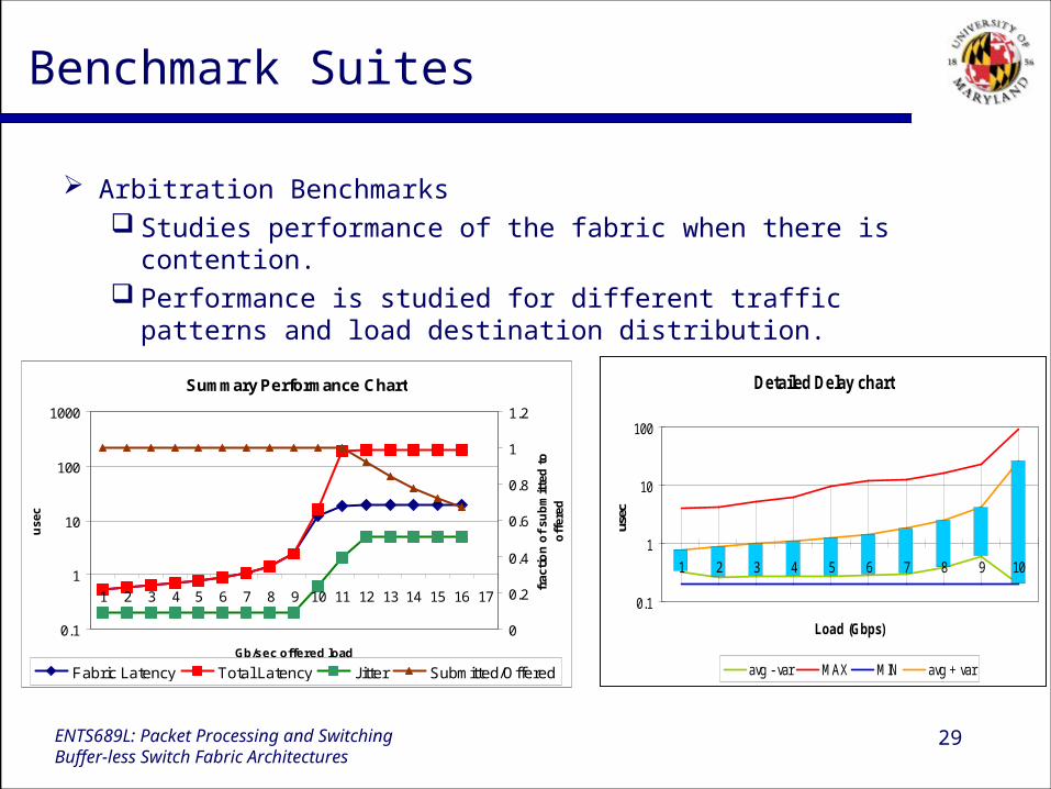
Arbitration Benchmarks Studies performance of the fabric when there is contention. Performance is studied for different traffic patterns and load
destination distribution.
Summary Performance Chart
0.1
1
10
100
1000
1 2 3 4 5 6 7 8 9 10 11 12 13 14 15 16 17
Gb/sec offered load
use
c
0
0.2
0.4
0.6
0.8
1
1.2
frac
tio
n o
f su
bm
itte
d t
o
off
ered
Fabric Latency Total Latency Jitter Submitted/Offered
Detailed Delay chart
0.1
1
10
100
1 2 3 4 5 6 7 8 9 10
Load (Gbps)us
ec
avg - var MAX MIN avg + var
Recommended