1
Ensemble Learning: An Introduction
Adapted from Slides by Tan, Steinbach, Kumar
2
General Idea
OriginalTraining data
....D1D2 Dt-1 Dt
D
Step 1:Create Multiple
Data Sets
C1 C2 Ct -1 Ct
Step 2:Build Multiple
Classifiers
C*Step 3:
CombineClassifiers
3
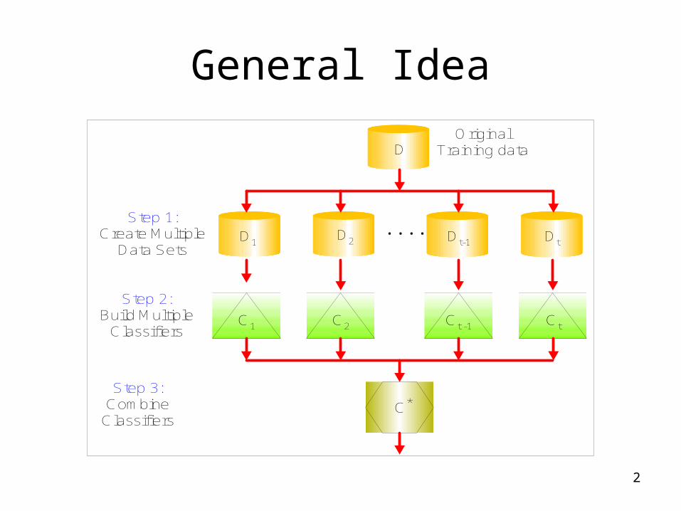
Why does it work?
• Suppose there are 25 base classifiers– Each classifier has error rate, = 0.35– Assume classifiers are independent– Probability that the ensemble classifier makes
a wrong prediction:
25
13
25 06.0)1(25
i
ii
i
4
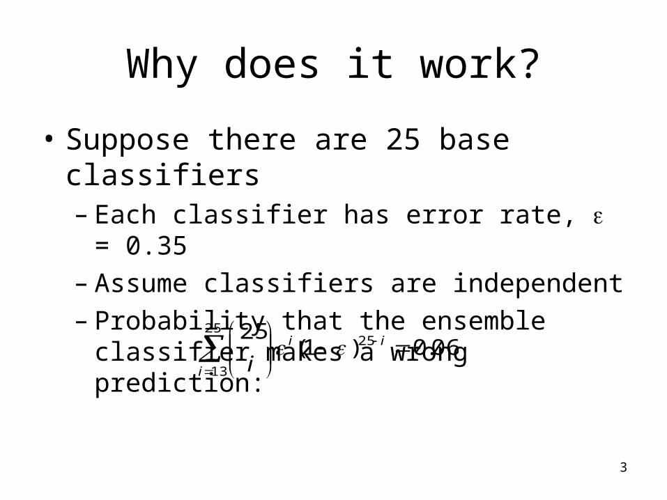
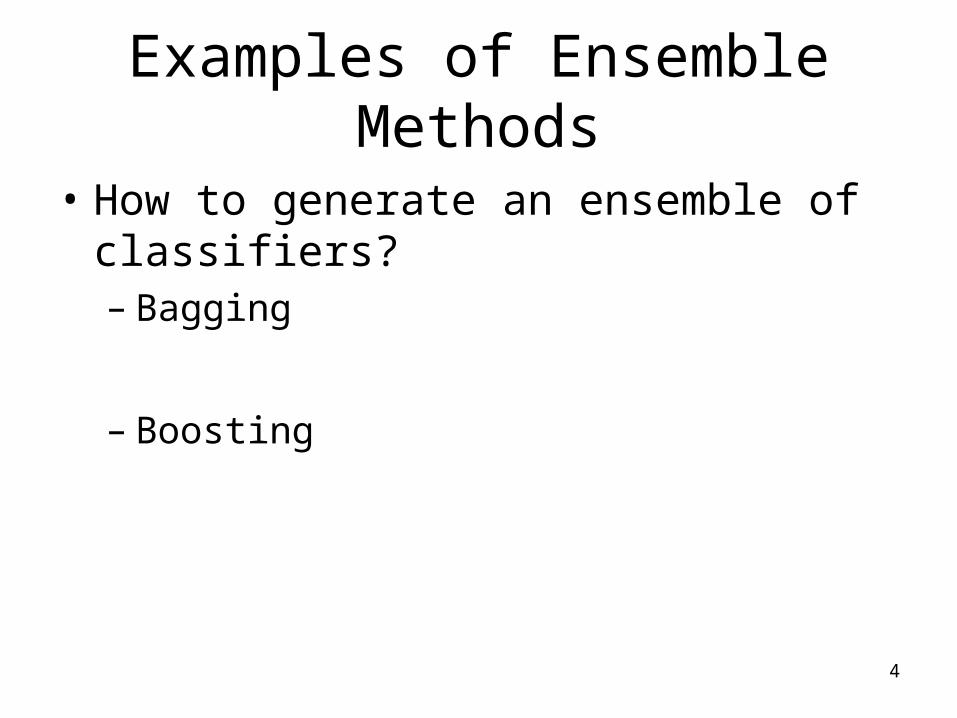
Examples of Ensemble Methods
• How to generate an ensemble of classifiers?– Bagging
– Boosting
5
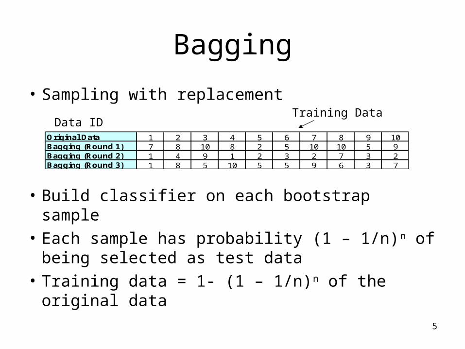
Bagging
• Sampling with replacement
• Build classifier on each bootstrap sample• Each sample has probability (1 – 1/n)n of being
selected as test data• Training data = 1- (1 – 1/n)n of the original data
Original Data 1 2 3 4 5 6 7 8 9 10Bagging (Round 1) 7 8 10 8 2 5 10 10 5 9Bagging (Round 2) 1 4 9 1 2 3 2 7 3 2Bagging (Round 3) 1 8 5 10 5 5 9 6 3 7
Training DataData ID
66
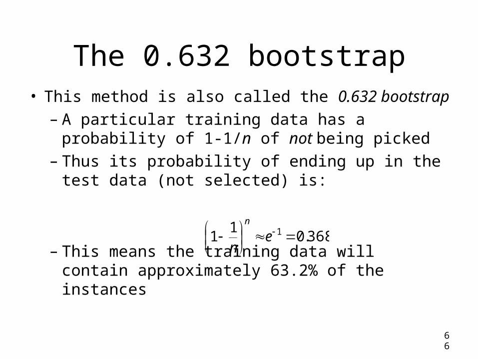
The 0.632 bootstrap• This method is also called the 0.632 bootstrap
– A particular training data has a probability of 1-1/n of not being picked
– Thus its probability of ending up in the test data (not selected) is:
– This means the training data will contain approximately 63.2% of the instances
368.01
1 1
e
n
n
7
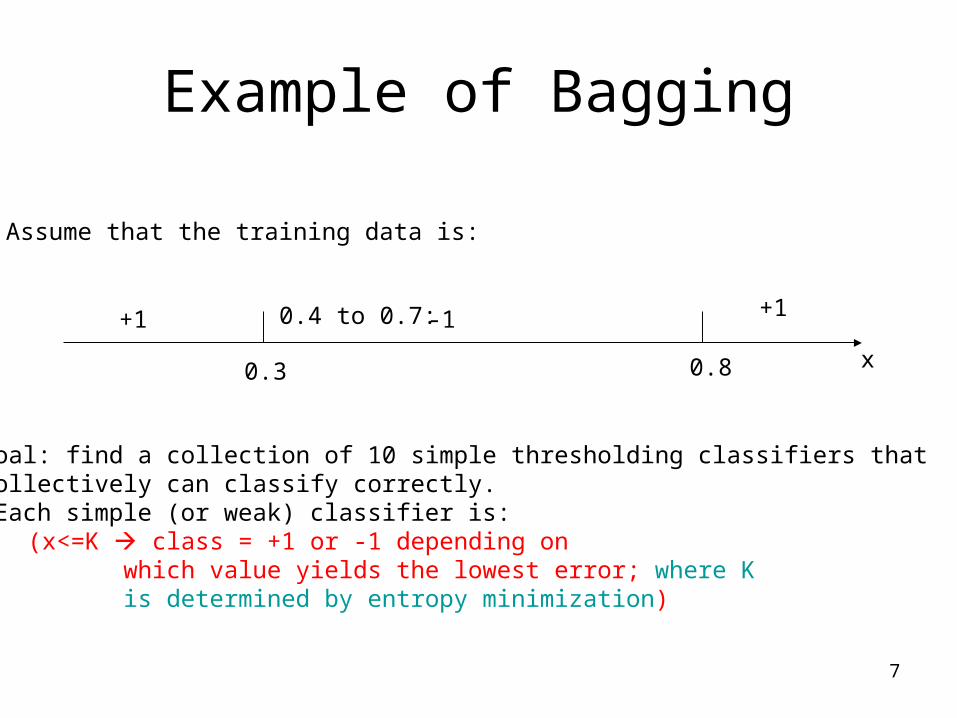
Example of Bagging
0.3 0.8 x
+1 +1-1
Assume that the training data is:
0.4 to 0.7:
Goal: find a collection of 10 simple thresholding classifiers that collectively can classify correctly.-Each simple (or weak) classifier is:
(x<=K class = +1 or -1 depending on which value yields the lowest error; where Kis determined by entropy minimization)
8
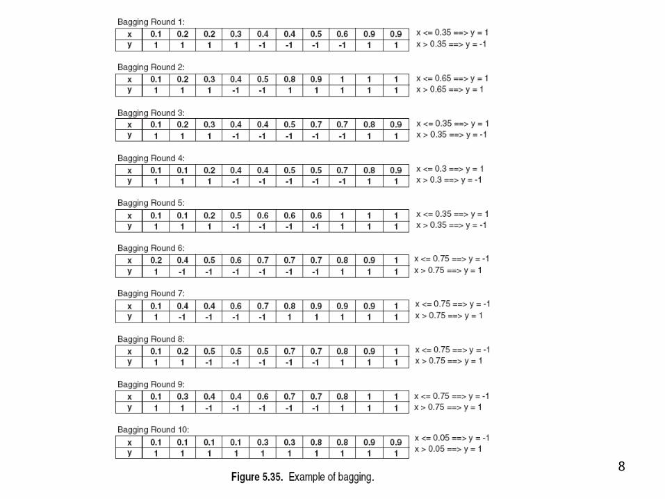
9
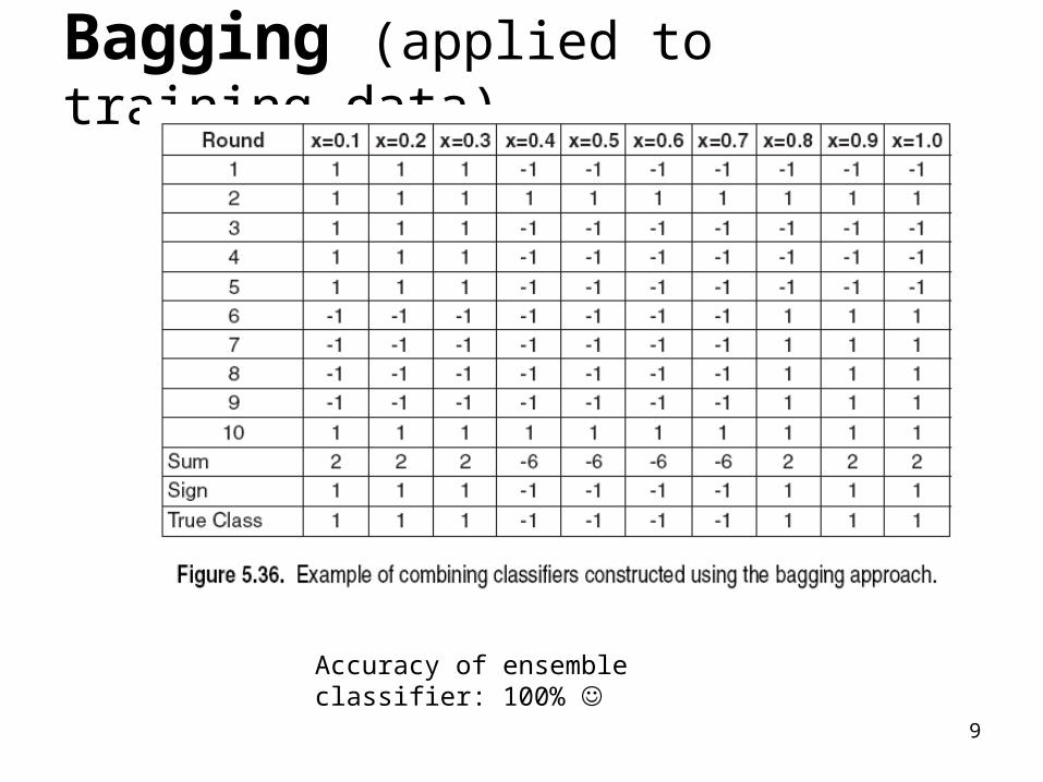
Bagging (applied to training data)
Accuracy of ensemble classifier: 100%
10
Bagging- Summary
• Works well if the base classifiers are unstable (complement each other)
• Increased accuracy because it reduces the variance of the individual classifier
• Does not focus on any particular instance of the training data– Therefore, less susceptible to model over-
fitting when applied to noisy data• What if we want to focus on a particular
instances of training data?
11
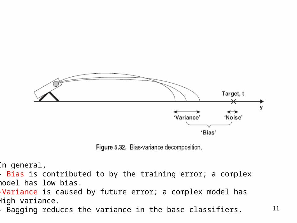
In general, - Bias is contributed to by the training error; a complex model has low bias.-Variance is caused by future error; a complex model hasHigh variance.- Bagging reduces the variance in the base classifiers.
12
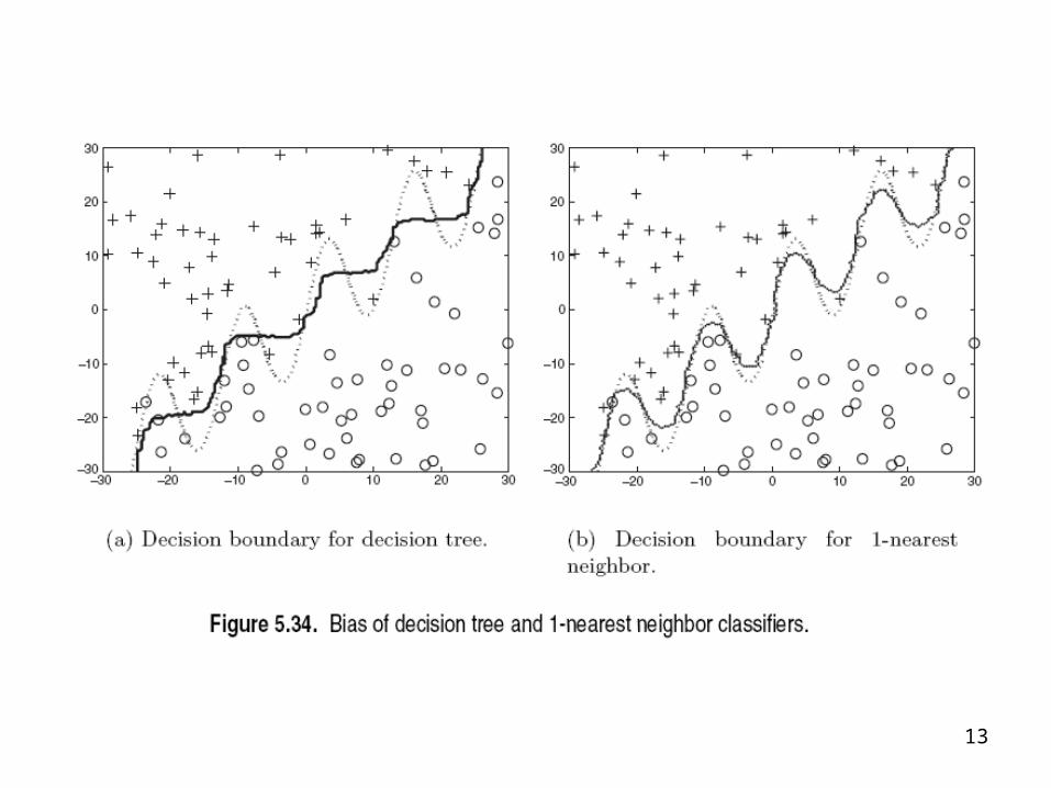
13
14
Boosting
• An iterative procedure to adaptively change distribution of training data by focusing more on previously misclassified records– Initially, all N records are assigned equal
weights– Unlike bagging, weights may change at the
end of a boosting round
15
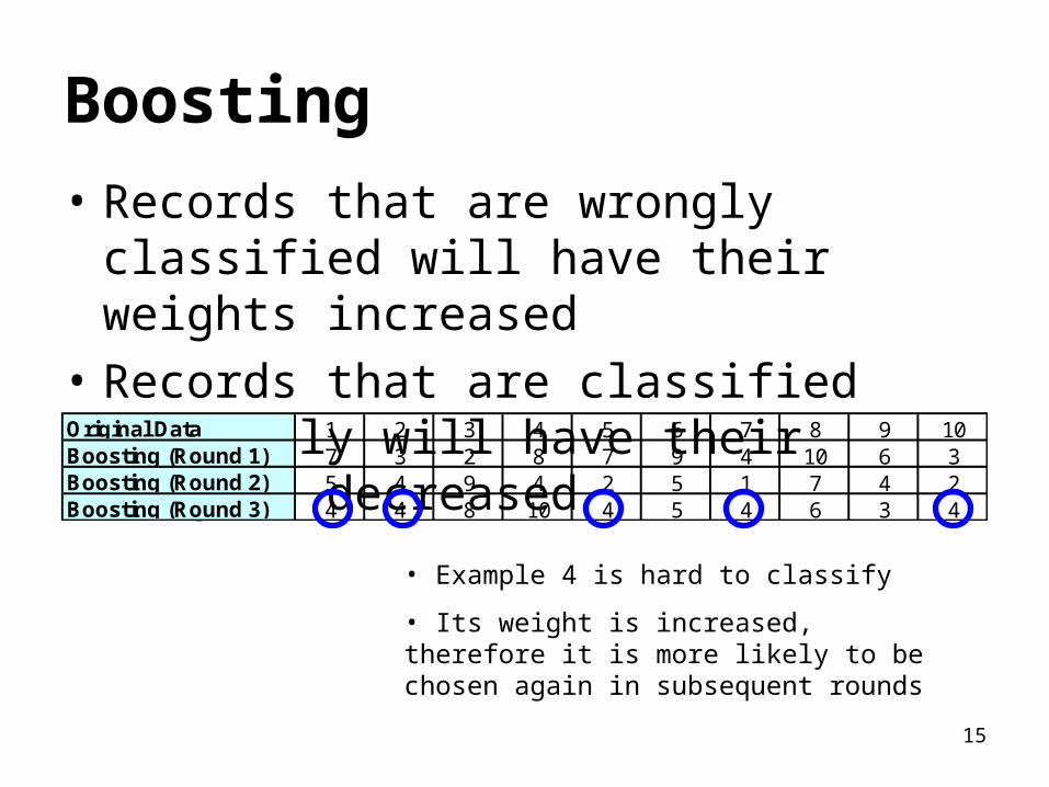
Boosting
• Records that are wrongly classified will have their weights increased
• Records that are classified correctly will have their weights decreased
Original Data 1 2 3 4 5 6 7 8 9 10Boosting (Round 1) 7 3 2 8 7 9 4 10 6 3Boosting (Round 2) 5 4 9 4 2 5 1 7 4 2Boosting (Round 3) 4 4 8 10 4 5 4 6 3 4
• Example 4 is hard to classify
• Its weight is increased, therefore it is more likely to be chosen again in subsequent rounds
16
Boosting• Equal weights are assigned to each training
instance (1/d for round 1) at first• After a classifier Ci is learned, the weights are
adjusted to allow the subsequent classifier Ci+1 to “pay more attention” to data that were
misclassified by Ci.• Final boosted classifier C* combines the
votes of each individual classifier– Weight of each classifier’s vote is a function of its
accuracy• Adaboost – popular boosting algorithm
17
Adaboost (Adaptive Boost)
• Input:– Training set D containing N instances– T rounds– A classification learning scheme
• Output: – A composite model
18
Adaboost: Training Phase • Training data D contain N labeled data (X1,y1),
(X2,y2 ), (X3,y3),….(XN,yN)• Initially assign equal weight 1/d to each data• To generate T base classifiers, we need T
rounds or iterations• Round i, data from D are sampled with
replacement , to form Di (size N)• Each data’s chance of being selected in the next
rounds depends on its weight– Each time the new sample is generated directly from
the training data D with different sampling probability according to the weights; these weights are not zero
19
Adaboost: Training Phase
• Base classifier Ci, is derived from training data of Di
• Error of Ci is tested using Di
• Weights of training data are adjusted depending on how they were classified– Correctly classified: Decrease weight– Incorrectly classified: Increase weight
• Weight of a data indicates how hard it is to classify it (directly proportional)
20
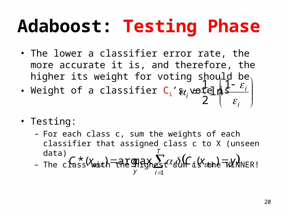
Adaboost: Testing Phase• The lower a classifier error rate, the more accurate it is,
and therefore, the higher its weight for voting should be
• Weight of a classifier Ci’s vote is
• Testing: – For each class c, sum the weights of each classifier that
assigned class c to X (unseen data)– The class with the highest sum is the WINNER!
i
ii
1ln
2
1
T
itestii
ytest yxCxC
1
)(maxarg)(*
21
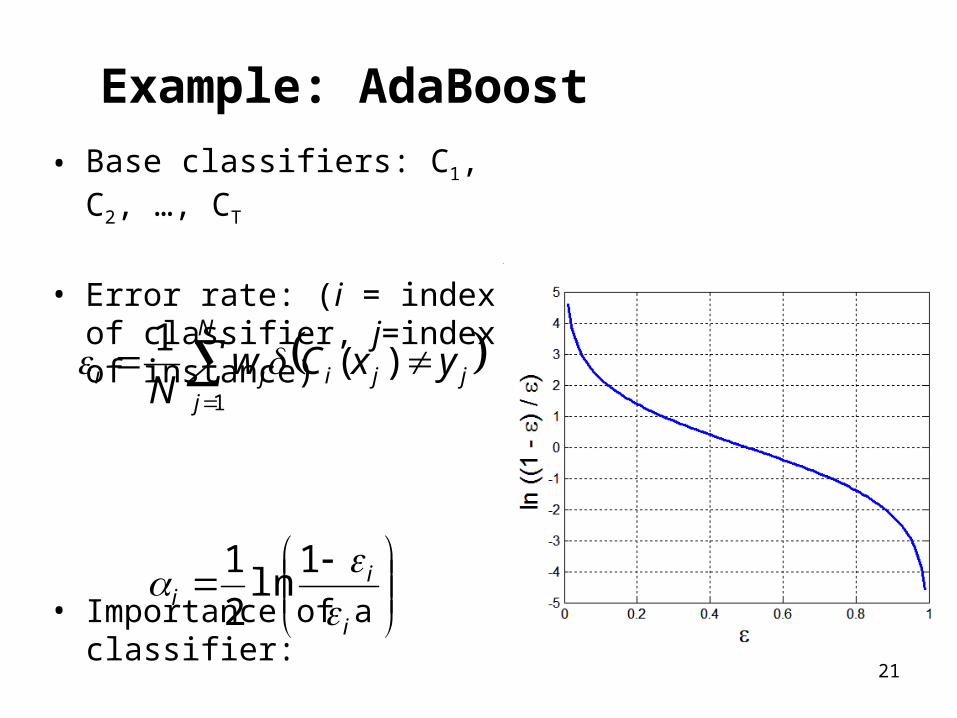
Example: AdaBoost
• Base classifiers: C1, C2, …, CT
• Error rate: (i = index of classifier, j=index of instance)
• Importance of a classifier:
N
jjjiji yxCw
N 1
)(1
i
ii
1ln
2
1
22
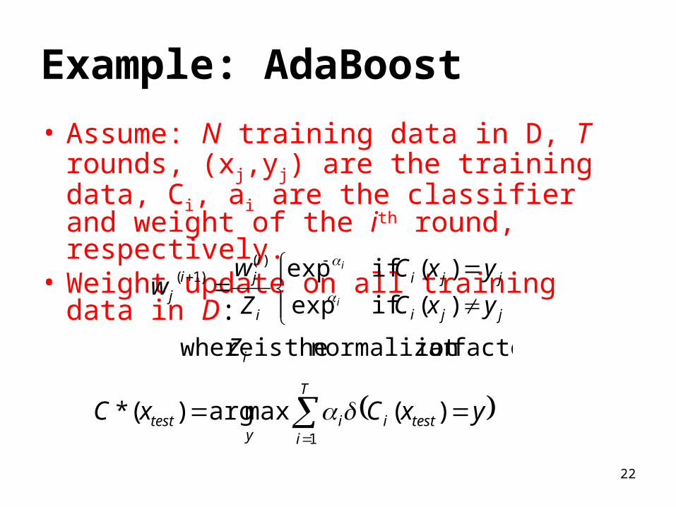
Example: AdaBoost
• Assume: N training data in D, T rounds, (xj,yj) are the training data, Ci, ai are the classifier and weight of the ith round, respectively.
• Weight update on all training data in D:
factorion normalizat theis where
)( ifexp
)( ifexp)()1(
i
jji
jji
i
iji
j
Z
yxC
yxC
Z
ww
i
i
T
itestii
ytest yxCxC
1
)(maxarg)(*
23
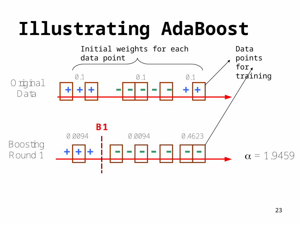
BoostingRound 1 + + + -- - - - - -
0.0094 0.0094 0.4623B1
= 1.9459
Illustrating AdaBoostData points for training
Initial weights for each data point
OriginalData + + + -- - - - + +
0.1 0.1 0.1
24
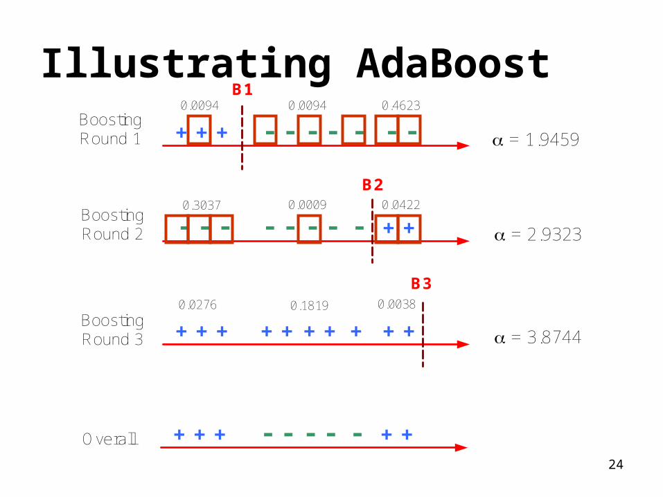
Illustrating AdaBoostBoostingRound 1 + + + -- - - - - -
BoostingRound 2 - - - -- - - - + +
BoostingRound 3 + + + ++ + + + + +
Overall + + + -- - - - + +
0.0094 0.0094 0.4623
0.3037 0.0009 0.0422
0.0276 0.1819 0.0038
B1
B2
B3
= 1.9459
= 2.9323
= 3.8744
25
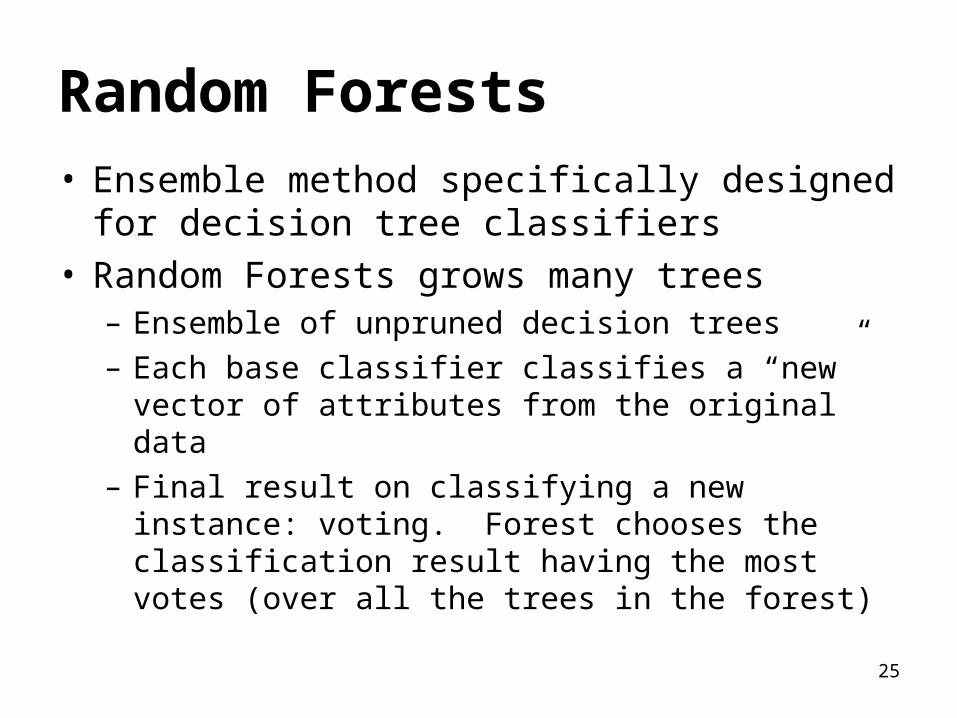
Random Forests• Ensemble method specifically designed for
decision tree classifiers• Random Forests grows many trees
– Ensemble of unpruned decision trees– Each base classifier classifies a “new” vector of
attributes from the original data– Final result on classifying a new instance: voting.
Forest chooses the classification result having the most votes (over all the trees in the forest)
26
Random Forests
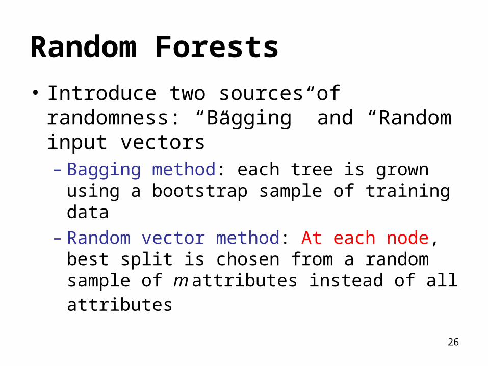
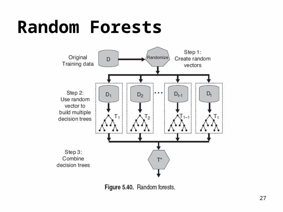
• Introduce two sources of randomness: “Bagging” and “Random input vectors”– Bagging method: each tree is grown using a
bootstrap sample of training data– Random vector method: At each node, best
split is chosen from a random sample of m
attributes instead of all attributes
27
Random Forests
28
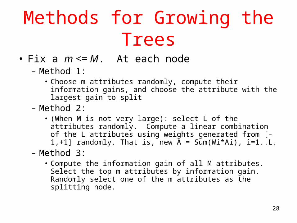
Methods for Growing the Trees
• Fix a m <= M. At each node– Method 1:
• Choose m attributes randomly, compute their information gains, and choose the attribute with the largest gain to split
– Method 2:• (When M is not very large): select L of the attributes
randomly. Compute a linear combination of the L attributes using weights generated from [-1,+1] randomly. That is, new A = Sum(Wi*Ai), i=1..L.
– Method 3: • Compute the information gain of all M attributes. Select the
top m attributes by information gain. Randomly select one of the m attributes as the splitting node.
29
Random Forest Algorithm: method 1 in previous slide• M input features in training data, a number
m<<M is specified such that at each node, m features are selected at random out of the M and the best split on these m features is used to split the node. (In weather data, M=4, and m is between 1 and 4)
• m is held constant during the forest growing• Each tree is grown to the largest extent possible
(deep tree, overfit easily), and there is no pruning
30
Generalization Error of Random Forests (page 291 of Tan book)
• It can be proven that the generalization Error <= (1-s2)/s2, is the average correlation among the trees– s is the strength of the tree classifiers
• Strength is defined as how certain the classification results are on the training data on average
• How certain is measured Pr(C1|X)-Pr(C2-X), where C1, C2 are class values of two highest probability in decreasing order for input instance X.
• Thus, higher diversity and accuracy is good for performance
Recommended
![Chapter DM:II (continued) - webis.de · Cluster Evaluation [Tan/Steinbach/Kumar 2005] Random points DM:II-200 Cluster Analysis ©STEIN 2006-2019](https://img.pdfslide.us/doc/110x75/5e0bb0aabeb12f5aad2f8024/chapter-dmii-continued-webisde-cluster-evaluation-tansteinbachkumar-2005.jpg)