arX
iv:1
409.
3307
v1 [
cs.S
Y]
11 S
ep 2
014
1
A Proximal Dual Consensus ADMM Methodfor Multi-Agent Constrained Optimization
Tsung-Hui Chang⋆, Member, IEEE
Abstract
This paper studies efficient distributed optimization methods for multi-agent networks. Specifically,we consider a convex optimization problem with a globally coupled linear equality constraint and localpolyhedra constraints, and develop distributed optimization methods based on the alternating directionmethod of multipliers (ADMM). The considered problem has many applications in machine learningand smart grid control problems. Due to the presence of the polyhedra constraints, agents in the existingmethods have to deal with polyhedra constrained subproblems at each iteration. One of the key issuesis that projection onto a polyhedra constraint is not trivial, which prohibits from closed-form solutionsor the use of simple algorithms for solving these subproblems. In this paper, by judiciously integratingthe proximal minimization method with ADMM, we propose a newdistributed optimization methodwhere the polyhedra constraints are handled softly as penalty terms in the subproblems. This makes thesubproblems efficiently solvable and consequently reducesthe overall computation time. Furthermore,we propose a randomized counterpart that is robust against randomly ON/OFF agents and imperfectcommunication links. We analytically show that both the proposed methods have a worst-caseO(1/k)
convergence rate, wherek is the iteration number. Numerical results show that the proposed methodsoffer considerably lower computation time than the existing distributed ADMM method.
Keywords− Distributed optimization, ADMM, ConsensusEDICS: OPT-DOPT, MLR-DIST, NET-DISP, SPC-APPL.
The work of Tsung-Hui Chang is supported by Ministry of Science and Technology, Taiwan (R.O.C.), under Grant NSC102-2221-E-011-005-MY3.
⋆Tsung-Hui Chang is the corresponding author. Address: Department of Electronic and Computer Engineering, NationalTaiwan University of Science and Technology, Taipei 10607,Taiwan, (R.O.C.). E-mail: [email protected].
September 12, 2014 DRAFT

2
I. INTRODUCTION
Multi-agent distributed optimization [1] has been of greatinterest due to applications in sensor networks
[2], cloud computing networks [3] and due to recent needs fordistributed large-scale signal processing
and machine learning tasks [4]. Distributed optimization methods are appealing because the agents access
and process local data and communicate with connecting neighbors only [1], thereby particularly suitable
for applications where the local data size is large and the network structure is complex. Many of the
problems can be formulated as the following optimization problem
(P) minx=[xT
1,...,xT
N ]T∈RNKF (x) ,
∑Ni=1 fi(xi) (1a)
s.t.∑N
i=1Eixi = q, (1b)
Cixi di,
xi ∈ Si,
, Xi, i = 1, . . . , N. (1c)
In (1), xi ∈ RK is a local control variable owned by agenti, fi is a local cost function,Ei ∈ R
L×K ,
q ∈ RL, Ci ∈ R
P×K, di ∈ RP andSi ⊆ R
K are locally known data matrices (vectors) and constraint set,
respectively. The constraint (1b) is a global constraint which couples all thexi’s; while eachXi in (1c) is
a local constraint set of agenti which consists of a simple constraint setSi (in the sense that projection
onto Si is easy to implement) and a polyhedra constraintCixi di. It is assumed that each agenti
knows onlyfi, Ei, Xi andq, and the agents collaborate to solve the coupled problem(P). Examples of
(P) include the basis pursuit (BP) [5] and LASSO problems [6] in machine learning, the power flow and
load control problems in smart grid [7], the network flow problem [8] and the coordinated transmission
design problem in communication networks [9], to name a few.
Various distributed optimization methods have been proposed in the literature for solving problems
with the form of (P). For example, the consensus subgradient methods [10]–[13]can be employed to
handle(P) by solving its Lagrange dual problem [1]. The consensus subgradient methods are simple to
implement, but the convergence rate is slow. In view of this,the alternating direction method of multipliers
(ADMM) [14], [15] has been used for fast distributed consensus optimization [16]–[21]. Specifically, the
work [16] proposed a consensus ADMM (C-ADMM) method for solving a distributed LASSO problem.
The linear convergence rate of C-ADMM is further analyzed in[20], and later, in [21], C-ADMM is
extended to that with asynchronous updates. By assuming that a certain coloring scheme is available to
the network graph, the works in [17], [18] proposed several distributed ADMM (D-ADMM) methods
for solving problems with the same form as(P). The D-ADMM methods require each agent either to
September 12, 2014 DRAFT

3
update the variables sequentially (not in parallel) or to solve a min-max (saddle point) subproblem at each
iteration. In the recent work [19], the authors proposed a distributed optimization method, called dual
consensus ADMM (DC-ADMM), which solves(P) in a fully parallel manner over arbitrary networks
as long as the graph is connected. An inexact counterpart of DC-ADMM was also proposed in [19] for
achieving a low per-iteration complexity whenF is complex.
In this paper, we improve upon the works in [19] by presentingnew computationally efficient distributed
optimization methods for solving(P). Specifically, due to the presence of the polyhedra constraints
Cixi di in (1c), the agents in the existing methods have to solve a polyhedra constrained subproblem
at each iteration. Since projection onto the polyhedra constraint is not trivial, closed-form solutions are
not available and, moreover, simple algorithms such as the gradient projection method [22] cannot handle
this constrained subproblem efficiently. To overcome this issue, we propose in this paper a proximal DC-
ADMM (PDC-ADMM) method where each of the agents deals with a subproblem with simple constraints
only, which is therefore more efficiently implementable than DC-ADMM. This is made possible by the
use of the proximal minimization method [14, Sec. 3.4.3] to deal with the dual variables associated with
the polyhedra constrains, so that the constraints can be softly handled as penalty terms in the subproblems.
Our contributions are summarized as follows.
• We propose a new PDC-ADMM method, and show that the proposed method converges to an
optimal solution of(P) with a worst-caseO(1/k) convergence rate, wherek is the iteration number.
Numerical results will show that the proposed PDC-ADMM method exhibits a significantly lower
computation time than DC-ADMM in [19].
• We further our study by presenting a randomized PDC-ADMM method that is tolerable to randomly
ON/OFF agents and robust against imperfect communication links. We show that the proposed
randomized PDC-ADMM method is convergent to an optimal solution of (P) in the mean, with a
worst-caseO(1/k) convergence rate.
The rest of this paper is organized as follows. Section II presents the applications, network model and
assumptions of(P). The PDC-ADMM method and the randomized PDC-ADMM method arepresented
in Section III and Section IV, respectively. Numerical results are presented in Section V and conclusions
are given in Section VI.
Notations: A 0 (≻ 0) means that matrixA is positive semidefinite (positive definite);a d
indicates that(d)i − (a)i ≥ 0 for all i, where(a)i means theith element of vectora. IK is theK ×K
identity matrix;1K is theK-dimensional all-one vector.‖a‖2 denotes the Euclidean norm of vectora,
September 12, 2014 DRAFT

4
‖a‖1 represents the 1-norm, and‖x‖2A , xTAx for someA 0; diaga1, . . . , aN is a diagonal matrix
with the ith diagonal element beingai. Notation⊗ denotes the Kronecker product.λmax(A) denotes the
maximum eigenvalue of the symmetric matrixA.
II. A PPLICATIONS, NETWORK MODEL AND ASSUMPTIONS
A. Applications
Problem (P) has applications in machine learning [4], [6], data communications [8], [9] and the
emerging smart grid systems [7], [13], [23], [24], to name a few. For example, whenfi(xi) = ‖xi‖22 ∀i,
(P) is the least-norm solution problem of the linear system∑N
i=1 Eixi = q; when fi(xi) = ‖xi‖1 ∀i,
(P) is the well-known basis pursuit (BP) problem [5], [17]; and if fi(xi) = ‖xi‖2 ∀i, then(P) is the BP
problem with group sparsity [6]. The LASSO problem can also be recast as the form of(P). Specifically,
consider a LASSO problem [6] with column partitioned data model [17, Fig. 1], [25],
minxi∈Xi,i=1,...,N
∥
∥
∥
∥
N∑
i=1
Aixi − b
∥
∥
∥
∥
2
2
+ λ
N∑
i=1
‖xi‖1, (2)
whereAi’s contain the training data vectors,b is a response signal andλ > 0 is a penalty parameter.
By definingx0 ,∑N
i=1 Aixi − b, one can equivalently write (2) as
minx0∈RL,
xi∈Si,i=1,...,N
‖x0‖22 + λ
N∑
i=1
‖xi‖1 (3a)
s.t.
N∑
i=1
Aixi − x0 = b, (3b)
Cixi di, i = 1, . . . , N, (3c)
which is exactly an instance of(P). The polyhedra constraintCixi di can rise, for example, in the
monotone curvature fitting problem [26]. Specifically, suppose that one wishes to fit a signal vector
b = [b(u1), . . . , b(uL)]T ∈ R
L over some fine grid of pointsu1, . . . , uL, using a set of monotone
vectorsgi = [gi(u1), . . . , gi(uL)]T , i = 1, . . . , N . Here, eachgi is modeled asgi = Aixi where
Ai = [ai(u1), . . . ,ai(uL)]T contains the basis vectors andxi is the fitting parameter vector. To impose
monotonicity ongi(u), one needs constraints of∂gi(uℓ)∂u
= (∂ai(uℓ)∂u
)Txi , cTi,ℓxi ≤ 0, ℓ = 1, . . . , L, if
gi(u) is non-increasing. This constitutes a polyhedra constraint Cixi , [ci,1, . . . , ci,L]Txi 0 on xi.
Readers may refer to [26] for more about constrained LASSO problems.
On the other hand, the load control problems [7], [13], [23] and microgrid control problems [24] in the
smart grid systems are also of the same form as(P). Specifically, consider that a utility company manages
September 12, 2014 DRAFT

5
the electricity consumption ofN customers for power balance. Letq ∈ RL denote the power supply
vector andφi(xi) ∈ RL be the power consumption vector of customeri’s load, wherexi ∈ R
K is the
load control variable. For many types of electricity loads (e.g., electrical vehicle (EV) and batteries), the
load consumptionφi can be expressed as a linear function ofxi [23], [24], i.e.,φi(xi) = Eixi, where
Ei ∈ RL×K is a mapping matrix. Besides, the variablesxi’s are often subject to some control constraints
(e.g., maximum/minimium charging rate and maximum capacity et al.), which can be represented by a
polyhedra constraintCixi di for someCi anddi. Then, the load control problem can be formulated
as
minx0∈RL,
xi∈RK ,i=1,...,N
U(x0) (4a)
s.t.
N∑
i=1
Eixi − x0 = q, (4b)
Cixi di, i = 1, . . . , N, (4c)
wherex0 is a slack variable andU is the cost function for power imbalance. Problem (4) is again an
instance of(P).
B. Network Model and Assumptions
We model the multi-agent network as a undirected graphG = V, E, whereV = 1, . . . , N is the
set of nodes (i.e, agents) andE is the set of edges. In particular, an edge(i, j) ∈ E if and only if agenti
and agentj are neighbors; that is, they can communicate and exchange messages with each other. Thus,
for each agenti, one can define the index subset of its neighbors asNi = j ∈ V | (i, j) ∈ E. Besides,
the adjacency matrix of the graphG is defined by the matrixW ∈ 0, 1N×N , where [W ]i,j = 1 if
(i, j) ∈ E and [W ]i,j = 0 otherwise. The degree matrix ofG is denoted byD = diag|N1|, . . . , |NN |.
We assume that
Assumption 1 The undirected graphG is connected.
Assumption 1 is essential for consensus optimization sinceit implies that any two agents in the network
can always influence each other in the long run. We also have the following assumption on the convexity
of (P).
Assumption 2 (P) is a convex problem, i.e.,fi’s are proper closed convex functions (possibly non-
smooth), andSi’s are closed convex sets; there is no duality gap between(P) and its Lagrange dual;
moreover, the minimum of(P) is attained and so is its optimal dual value.
September 12, 2014 DRAFT

6
III. PROPOSEDPROXIMAL DUAL CONSENSUSADMM M ETHOD
In the section, we propose a distributed optimization method for solving(P), referred to as the proximal
dual consensus ADMM (PDC-ADMM) method. We will compare the proposed PDC-ADMM method with
the existing DC-ADMM method in [19], and discuss the potential computational merit of the proposed
PDC-ADMM.
The proposed PDC-ADMM method considers the Lagrange dual of(P). Let us write(P) as follows
minxi∈Si,ri0,
∀i∈V
N∑
i=1
fi(xi) (5a)
s.t.N∑
i=1
Eixi = q, (5b)
Cixi + ri − di = 0 ∀i ∈ V, (5c)
whereri ∈ RP+, i ∈ V, are introduced slack variables. Denotey ∈ R
L as the Lagrange dual variable
associated with constraint (5b), andzi ∈ RP as the Lagrange dual variable associated with each of the
constraints in (5c). The Lagrange dual problem of (5) is equivalent to the following problem
miny∈RL,zi∈RP
∀i∈V
N∑
i=1
(
ϕi(y,zi) +1
NyTq + zT
i di
)
(6)
where
ϕi(y,zi) , maxxi∈Si,ri≥0
− fi(xi)− yTEixi − zT
i (Cixi + ri)
, (7)
for all i ∈ V. To enable multi-agent distributed optimization, we alloweach agenti to have a local copy
of the variabley, denoted byyi, while enforcing the distributedyi’s to be the same across the network
through proper consensus constraints. This is equivalent to reformulating (6) as the following problem
minyi,zi,si
tij∀i∈V
N∑
i=1
(
ϕi(yi,zi) +1
NyTi q + zT
i di
)
(8a)
s.t. yi = tij ∀j ∈ Ni, i ∈ V, (8b)
yj = tij ∀j ∈ Ni, i ∈ V, (8c)
zi = si, ∀i ∈ V, (8d)
wheretij andsi are slack variables. Constraints (8b) and (8c) are equivalent to the neighbor-wise
consensus constraints, i.e.,yi = yj ∀j ∈ Ni, i ∈ V. Under Assumption 1, neighbor-wise consensus is
equivalent to global consensus; thus (8) is equivalent to (6). It is worthwhile to note that, while constraint
September 12, 2014 DRAFT
7
(8d) looks redundant at this stage, it is a key step that constitutes the proposed method as will be clear
shortly.
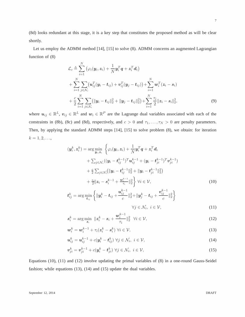
Let us employ the ADMM method [14], [15] to solve (8). ADMM concerns an augmented Lagrangian
function of (8)
Lc ,
N∑
i=1
(
ϕi(yi,zi) +1
NyTi q + zT
i di
)
+
N∑
i=1
∑
j∈Ni
(
uTij(yi − tij) + vT
ij(yj − tij))
+
N∑
i=1
wTi (zi − si)
+c
2
N∑
i=1
∑
j∈Ni
(
‖yi − tij‖22 + ‖yj − tij‖
22
)
+
N∑
i=1
τi2‖zi − si‖
22, (9)
whereuij ∈ RL, vij ∈ R
L andwi ∈ RP are the Lagrange dual variables associated with each of the
constraints in (8b), (8c) and (8d), respectively, andc > 0 and τ1, . . . , τN > 0 are penalty parameters.
Then, by applying the standard ADMM steps [14], [15] to solveproblem (8), we obtain: for iteration
k = 1, 2, . . .,
(yki ,z
ki ) = argmin
yi,zi
ϕi(yi,zi) +1
NyTi q + zT
i di
+∑
j∈Ni((yi − tk−1
ij )Tuk−1ij + (yi − tk−1
ji )Tvk−1ji )
+ c2
∑
j∈Ni
(
‖yi − tk−1ij ‖22 + ‖yi − tk−1
ji ‖22)
+ τi2‖zi − sk−1
i + wk−1
i
τi‖22
∀i ∈ V, (10)
tkij = argmintij
‖yki − tij +
uk−1ij
c‖22+‖yk
j − tij +vk−1ij
c‖22
∀j ∈ Ni, i ∈ V, (11)
ski = argminsi
‖zki − si +
wk−1i
τi‖22 ∀i ∈ V, (12)
wki = wk−1
i + τi(zki − ski ) ∀i ∈ V, (13)
ukij = uk−1
ij + c(yki − tkij) ∀j ∈ Ni, i ∈ V, (14)
vkji = vk−1
ji + c(yki − tkji) ∀j ∈ Ni, i ∈ V, (15)
Equations (10), (11) and (12) involve updating the primal variables of (8) in a one-round Gauss-Seidel
fashion; while equations (13), (14) and (15) update the dualvariables.
September 12, 2014 DRAFT
8
It is shown in Appendix A that
tkij = tkji =yki + yk
j
2, wk
i = 0, ski = zki , (16)
for all k and for all i, j. By (16), equations (10) to (15) can be simplified to the following steps
(yki ,z
ki ) = argmin
yi,zi
ϕi(yi,zi) +1
NyTi q + zT
i di
+ yTi
∑
j∈Ni(uk−1
ij + vk−1ji ) + c
∑
j∈Ni‖yi −
yk−1
i +yk−1
j
2 ‖22
+ τi2‖zi − zk−1
i ‖22
∀i ∈ V, (17)
ukij = uk−1
ij + c(yki −
yki +yk
j
2 ) ∀j ∈ Ni, i ∈ V, (18)
vkji = vk−1
ji + c(yki −
yki +yk
j
2 ) ∀j ∈ Ni, i ∈ V. (19)
By letting
pki ,
∑
j∈Ni(uk
ij + vkji) ∀i ∈ V, (20)
(18) and (19) reduce to
pki = pk−1
i + c∑
j∈Ni(yk
i − ykj ) ∀i ∈ V. (21)
On the other hand, note that the subproblem in (17) is a strongly convex problem. However, it is not
easy to handle as subproblem (17) is in fact a min-max (saddlepoint) problem (see the definition ofϕi
in (7)). Fortunately, by applying the minimax theorem [27, Proposition 2.6.2] and exploiting the strong
convexity of (17) with respect to(yi,zi), one may avoid solving the min-max problem (17) directly. As
we show in Appendix B,(yki ,z
ki ) of subproblem (17) can be conveniently obtained in closed-form as
follows
yki = 1
2|Ni|(∑
j∈Ni(yk−1
i + yk−1j )− 1
cpk−1i
+ 1c(Eix
ki −
1Nq))
, (22a)
zki = zk−1
i +1
τi(Cix
ki + rki − di). (22b)
where(xki , r
ki ) is given by an solution to the following quadratic program (QP)
(xki , r
ki )=arg min
xi∈Si,ri0
fi(xi)+c
4|Ni|
∥
∥
1c(Eixi −
1Nq) − 1
cpki
+∑
j∈Ni(yk−1
i + yk−1j )
∥
∥
2
2
+ 12τi
‖Cixi + ri − di + τizk−1i ‖22
. (23)
September 12, 2014 DRAFT

9
As also shown in Appendix B, the dummy constraintzi = si in (8d) and the augmented term
τi2
∑Ni=1 ‖zi−si‖
22 in (9) are essential for arriving at (22) and (23). Since theyare equivalent to applying
the proximal minimization method [14, Sec. 3.4.3] to the variableszi’s in (8), we name the developed
method above the proximal DC-ADMM method. In Algorithm 1, wesummarize the proposed PDC-
ADMM method. Note that the PDC-ADMM method in Algorithm 1 is fully parallel and distributed
except that, in (29), each agenti requires to exchangeyki with its neighbors.
The PDC-ADMM method in Algorithm 1 is provably convergent, as stated in the following theorem.
Theorem 1 Suppose that Assumptions 1 and 2 hold. Let(x⋆, r⋆i Ni=1) and(y⋆,z⋆), be a pair of optimal
primal-dual solution of(5) (i.e., (P)), wherex⋆ = [(x⋆1)
T , . . . , (x⋆N )T ]T andz⋆ = [(z⋆
1)T , . . . , (z⋆
N )T ]T ,
and let u⋆ = u⋆ij (which stacks allu⋆
ij for all i, j) be an optimal dual variable of problem(8).
Moreover, let
xMi , 1
M
∑Mk=1 x
ki , rMi , 1
M
∑Mk=1 r
ki ∀i ∈ V, (24)
and xM = [(xM1 )T , . . . , (xM
N )T ]T , wherexki , r
ki
Ni=1 are generated by(26). Then, it holds that
|F (xM )− F (x⋆)|+ ‖N∑
i=1
EixMi − q‖2
+
N∑
i=1
‖CixMi + rMi − di‖2 ≤
(1 + δ)C1 + C2
M, (25)
whereδ , max‖y⋆‖2, ‖z⋆1‖2, . . . , ‖z
⋆N‖2, C1 ,
τi2 max‖a‖2≤
√N‖z0 − (z⋆ + a)‖2
Γ+ 1
c‖u1 − u⋆‖22 +
c2 max‖a‖2≤1 ‖y
0 − 1N ⊗ (y⋆ +a)‖2Q andC2 ,τi2 ‖z
0 − z⋆‖2Γ+ c
2‖y0 −1N ⊗y⋆‖2Q + 1
c‖u1 −u⋆‖22 are
constants, in whichΓ , diagτ1, . . . , τN andQ , (D +W )⊗ IL 0.
The proof is presented in Appendix C. Theorem 1 implies that the proposed PDC-ADMM method
asymptotically converges to an optimal solution of(P) with a worst-caseO(1/k) convergence rate.
As discussed in Appendix B, if one removes the dummy constraint zi = si from (8) and the augmented
term∑N
i=1τi2 ‖zi − si‖
22 from (9), then the above development of PDC-ADMM reduces to the existing
DC-ADMM method in [19]. The DC-ADMM method is presented in Algorithm 2. Two important remarks
on the comparison between PDC-ADMM and DC-ADMM are in order.
Remark 1 As one can see from Algorithm 1 and Algorithm 2, except for thestep in (28), the major
difference between PDC-ADMM and DC-ADMM lies in (26) and (30). In particular, subproblem (30) is
explicitly constrained by the polyhedra constraintCixi di; whereas, subproblem (26) has the simple
constraint setsxi ∈ Si andri 0 only, though (26) has an additional penalty term12τi ‖Cixi+ri−di+
September 12, 2014 DRAFT

10
Algorithm 1 PDC-ADMM for solving (P)
1: Given initial variablesx(0)i ∈ R
K , y(0)i ∈ R
L, z(0)i ∈ R
P , r(0)i ∈ RP andp(0)
i = 0 for each agenti,
i ∈ V. Setk = 1.
2: repeat
3: For all i ∈ V (in parallel),
(xki , r
ki )=arg min
xi∈Si,ri0
fi(xi)+c
4|Ni|
∥
∥
1c(Eixi
− 1Nq)− 1
cpk−1i +
∑
j∈Ni(yk−1
i + yk−1j )
∥
∥
2
2
+ 12τi
‖Cixi + ri − di + τizk−1i ‖22
, (26)
yki = 1
2|Ni|(∑
j∈Ni(yk−1
i + yk−1j )− 1
cpk−1i
+ 1c(Eix
ki −
1Nq))
, (27)
zki = zk−1
i +1
τi(Cix
ki + rki − di), (28)
pki = pk−1
i + c∑
j∈Ni(yk
i − ykj ). (29)
4: Set k = k + 1.
5: until a predefined stopping criterion is satisfied.
τizk−1i ‖22. In fact, one can show that, ifτi = 0, then the penalty term functions as an indicator function
enforcingCixi + ri − di = 0 (which is equivalent toCixi di as ri 0). Therefore, (26) boils
down to (30) whenτi = 0; that is to say, the proposed PDC-ADMM can be regarded as a generalization
of DC-ADMM, in the sense that the local polyhedra constraints are handled “softly” depending on the
parameterτi.
Remark 2 More importantly, PDC-ADMM provides extra flexibility for efficient implementation. In
particular, because bothSi and the non-negative orthant are simple to project, subproblem (26) in PDC-
ADMM can be efficiently handled by several simple algorithms. For example, due to the special problem
structure, subproblem (26) can be efficiently handled by theblock coordinate descent (BCD) type methods
[28], [22, Sec. 2.7.1] such as the block successive upper bound minimization (BSUM) method [29].
Specifically, by the BSUM method, one may updatexi andri iteratively in a Gauss-Seidel fashion, i.e.,
September 12, 2014 DRAFT

11
Algorithm 2 DC-ADMM for solving (P) [19]
1: Given initial variablesx(0)i ∈ R
K , y(0)i ∈ R
L andp(0)i = 0 for each agenti, i ∈ V. Setk = 1.
2: repeat
3: For all i ∈ V (in parallel),
xki =arg min
xi∈Si
fi(xi) +c
4|Ni|
∥
∥
1c(Eixi −
1Nq)
− 1cpk−1i +
∑
j∈Ni(yk−1
i + yk−1j )
∥
∥
2
2
s.t. Cixi di, (30)
yki = 1
2|Ni|(∑
j∈Ni(yk−1
i + yk−1j )− 1
cpk−1i
+ 1c(Eix
ki −
1Nq))
, (31)
pki =pk−1
i + c∑
j∈Ni(yk
i − ykj ). (32)
4: Set k = k + 1.
5: until a predefined stopping criterion is satisfied.
for iteration ℓ = 1, 2, . . . ,
xℓ+1i =arg min
xi∈Si
ui(xi; xℓi , r
ℓi ), (33a)
rℓ+1i = maxdi − czk−1
i −Cixℓ+1i ,0, (33b)
whereui(xi; xℓi , r
ℓi ) is a “locally tight” upper bound function for the objective function of (26) given
(xℓi , r
ℓi ), and is chosen judiciously so that (33a) can yield simple closed-form solutions; see [29] for
more details. Since the update ofri in (33b) is also in closed-form, the BSUM method for solving (26)
is computationally efficient. Besides, the (accelerated) gradient projection methods (such as FISTA [30])
can also be employed to solve subproblem (26) efficiently.
On the contrary, since projection onto the polyhedra constraint Cixi di has no closed-form and
is not trivial to implement in general, previously mentioned algorithms cannot deal with subproblem
(30) efficiently. Although primal-dual algorithms [31] (such as ADMM [14]) can be applied, they are
arguably more complex. In particular, since one usually requires a high-accuracy solution to subproblem
(30), DC-ADMM is more time consuming than the proposed PDC-ADMM, as will be demonstrated in
Section V.
September 12, 2014 DRAFT
12
IV. RANDOMIZED PDC-ADMM
The PDC-ADMM method in Algorithm 1 requires all agents to be active, updating variables and
exchanging messages at every iterationk. In this section, we develop an randomized PDC-ADMM method
which is applicable to networks with randomly ON/OFF agentsand non-ideal communication links1.
Specifically, assume that, at each iteration (e.g., time epoch), each agent has a probability, sayαi ∈ (0, 1],
to be ON (active), and moreover, for each link(i, j) ∈ E , there is a probabilitype ∈ (0, 1] to have link
failure (i.e., agenti and agentj cannot successfully exchange messages due to, e.g., communication
errors). So, the probability that agenti and agentj are both active and able to exchange messages is
given byβij = αiαj(1− pe). If this happens, we say that link(i, j) ∈ E is active at the iteration.
For each iterationk, let Ωk ⊆ V be the set of active agents and letΨk ⊆ (i, j) ∈ E |i, j ∈ Ωk be
the set of active edges. Then, at each iterationk of the proposed randomized PDC-ADMM method, only
active agents perform local variable update and they exchange message only with active neighboring
agents with active links in between. The proposed randomized PDC-ADMM method is presented in
Algorithm 3.
Note that, similar to (18), (19) and (21), update (38) equivalently corresponds to
ukij =
uk−1ij + c(yk
i − tkij) if (i, j) ∈ Ψk,
uk−1ij , otherwise,
(40)
vkji =
vk−1ji + c(yk
i − tkji) if (i, j) ∈ Ψk,
vk−1ji , otherwise.
(41)
Besides, ifΩk = V andΨk = E for all k, then the randomized PDC-ADMM reduces to the (deterministic)
PDC-ADMM in Algorithm 1.
There are two key differences between the randomized PDC-ADMM method and its deterministic
counterpart in Algorithm 1. Firstly, in addition to(xki , r
ki ,y
ki ,z
ki ,p
ki ), each agenti in randomized PDC-
ADMM also requires to maintain variablestij , j ∈ Ni. Secondly, variables(xki , r
ki ,y
ki ,z
ki ,p
ki ) are
updated only ifi ∈ Ωk and variables(tkij, ukij ,v
kji) are updated only if(i, j) ∈ Ψk. Therefore, the
randomized PDC-ADMM method is robust against randomly ON/OFF agents and link failures. The
convergence result of randomized PDC-ADMM is given by the following theorem.
Theorem 2 Suppose that Assumptions 1 and 2 hold. Besides, assume that each agenti has an active
probability αi ∈ (0, 1] and, for each link(i, j) ∈ E , there is a link failure probabilitype ∈ (0, 1]. Let
1The proposed randomized method and analysis techniques areinspired by the recent works in [21], [32].
September 12, 2014 DRAFT

13
Algorithm 3 Randomized PDC-ADMM for solving(P)
1: Given initial variablesx0i ∈ R
K , y0i ∈ R
L, z0i ∈ R
P , r0i ∈ RP , p0
i = 0 and
t0ij =y0
i+y0
j
2 ∀j ∈ Ni,
for each agenti, i ∈ V. Setk = 1.
2: repeat
3: For all i ∈ Ωk (in parallel),
(xki , r
ki )=arg min
xi∈Si,ri0
fi(xi)+c
4|Ni|
∥
∥
1c(Eixi −
1Nq)− 1
cpk−1i + 2
∑
j∈Nitk−1ij
+ 12τi
‖Cixi + ri − di + τizk−1i ‖22
, (34)
yki = 1
2|Ni|(
2∑
j∈Nitk−1ij − 1
cpk−1i + 1
c(Eix
ki −
1Nq))
, (35)
zki = zk−1
i + 1τi(Cix
ki + rki − di), (36)
tkij =
yki +yk
j
2 if (i, j) ∈ Ψk,
tk−1ij , otherwise,
(37)
pki = pk−1
i + 2c∑
j|(i,j)∈Ψk(yki − tkij); (38)
whereas for alli /∈ Ωk (in parallel)
xki = xk−1
i , rki = rk−1i , yk
i = yk−1i , zk
i = zk−1i ,
tkij = tk−1ij ∀j ∈ Ni, pk
i = pk−1i . (39)
4: Set k = k + 1.
5: until a predefined stopping criterion is satisfied.
(x⋆, r⋆i Ni=1) and(y⋆,z⋆), be a pair of optimal primal-dual solution of(5) (i.e., (P)), and letu⋆ = u⋆
ij
be an optimal dual variable of problem(8). Moreover, let
xMi , 1
M
∑Mk=1 x
ki , rMi , 1
M
∑Mk=1 r
ki ∀i ∈ V, (42)
wherexki , r
ki
Ni=1 are generated by(34). Then, it holds that
|E[F (xM )− F (x⋆)]|+ ‖E[N∑
i=1
EixMi − q]‖2 +
N∑
i=1
‖E[CixMi + rMi − di]‖2 ≤
(1 + δ)C1 + C2
M, (43)
whereδ is defined as in Theorem 1 andC1 and C2 are constants defined in(A.62) and (A.64).
September 12, 2014 DRAFT

14
The proof is presented in Appendix D. Theorem 2 implies that randomized PDC-ADMM can converge
to the optimal solution of(P) in the mean, with aO(1/k) worst-case convergence rate. It is worthwhile to
note that the constantsC1 andC2 depend on the agent active probability and the link failure probability. In
Section V, we will further investigate the impacts of these parameters on the convergence of randomized
PDC-ADMM by computer simulations.
V. NUMERICAL RESULTS
In this section, we present some numerical results to examine the performance of the proposed PDC-
ADMM and randomized PDC-ADMM methods. We consider the linearly constrained LASSO problem in
(2) and respectively apply DC-ADMM (Algorithm 2), PDC-ADMM(Algorithm 1) and randomized PDC-
ADMM (Algorithm 3) to handle the equivalent formulation (3). The ADMM method [14] is employed
to handle subproblem (30)2 in DC-ADMM (Algorithm 2). In particular,c1 > 0 is denoted as the penalty
parameter used in the ADMM method and the stopping criterionis based on the sum of dimension-
normalized primal and dual residuals [15, Section 3.3] which is denoted byǫ1 > 0. On the other hand,
the BSUM method (i.e., (33)) is used to handle subproblem (26) in PDC-ADMM (Algorithm 1) and,
similarly, subproblem (34) in randomized PDC-ADMM (Algorithm 3). Specifically, the upper bound
functionui(xi; xℓi , r
ℓi ) is obtained by considering the regularized first-order approximation of the smooth
componentg(xi, ri) ,c
4|Ni|∥
∥
1c(Eixi−
1Nq)− 1
cpk−1i +
∑
j∈Ni(yk−1
i +yk−1j )
∥
∥
2
2+ 1
2τi‖Cixi+ ri−di+
τizk−1i ‖22 in the objective function of (26), i.e.,
ui(xi; xℓi , r
ℓi ) = fi(xi) + (∇xg(x
ℓi , r
ℓi ))
T (xi − xℓi)
+βi2‖xi − xℓ
i‖22, (44)
whereβi = 0.4λmax(c
2|Ni|ETi Ei +
1τiCT
i Ci) is a penalty parameter3 and
∇xg(xℓi , r
ℓi ) =
(
c2|Ni|E
Ti Ei +
1τiCT
i Ci
)
xℓi
− c2|Ni|E
Ti (
1Nb+ 1
cpk−1i −
∑
j∈Ni(yk−1
i + yk−1j ))
+ 1τiCT
i (rℓi − di + τiz
k−1i ).
2Due to the page limit, the detailed implementation of ADMM for (30) is omitted here.
3Theoretically, it requires thatβi > λmax(c
2|Ni|E
T
i Ei +1
τiC
T
i Ci) so thatui(xi; xℓ
i , rℓ
i ) is an upper bound function of the
objective function of (26). However, we find in simulations that a smallerβi still works and may converge faster in practice.
September 12, 2014 DRAFT

15
With (44), the subproblem (33a) reduces to the well-known soft-thresholding operator [33], [34]. The
stopping criterion of the BSUM algorithm is based on the difference of variables in two consecutive
iterations, i.e.,ǫ2 ,
√
‖xℓi − xℓ−1
i ‖22 + ‖rℓi − rℓ−1i ‖22/(K + P ). Note that smallerǫ1 and ǫ2 imply that
the agents spend more efforts (computational time) in solving subproblems (30) and (26), respectively.
The stopping criteria of Algorithms 1 to 3 are based on the solution accuracyAcc = (obj(xk)− obj⋆)/obj⋆
and the feasibility for constraintsCixi di, i = 1, . . . , N , i.e., Feas =∑N
i=1
∑Pj=1max(Cix
ki −
di)j, 0/(NP ), whereobj(xk) denotes the objective value of (2) atxk, andobj⋆ is the optimal value of
(2) which was obtained byCVX [35].
The matricesAi’s, Ci’s and vectorsb and di’s in (2) are randomly generated. Moreover, it is set
that Si = RK for all i. The connected graphG was also randomly generated, following the method in
[36]. The average performance of all algorithms under test in Table I are obtained by averaging over 10
random problem instances of (2) and random graphs. The stopping criterion of all algorithms under test
is that the sum of solution accuracy (Acc) and feasibility (Feas) is less than10−4, i.e., Acc + Feas
≤ 10−4. The simulations are performed inMATLAB by a computer with 8 core CPUs and 8 GB RAM.
Example 1: We first consider the performance comparison between DC-ADMM and PDC-ADMM.
Table I(a) shows the comparison results forN = 50, K = 500, L = 100, P = 250 andλ = 10. For
PDC-ADMM, we simply setτ1 = · · · = τN , τ and τ = c. The penalty parametersc of the two
algorithms are respectively chosen so that the two algorithms can exhibit best convergence behaviors4.
One can see from Table I(a) that DC-ADMM (c = 0.01, c1 = 5, ǫ1 = 10−6)5 can achieve the stopping
conditionAcc + Feas ≤ 10−4 with an average iteration number37.7 but spends an average per-agent
computation time of 19.63 seconds. One should note that a naive way to reducing the computation time
of DC-ADMM is to reduce the solution accuracy of subproblem (30), i.e., increasingǫ1. As seen, DC-
ADMM with ǫ1 = 10−5 has a reduced per-agent computation time 9.87 seconds; however, the required
iteration number drastically increases to 980.1. By contrast, one can see from Table I(a) that the proposed
PDC-ADMM (c = τ = 0.01, ǫ2 = 10−6) can achieve the stopping condition with an average iteration
number55.9 and a much less (per-agent) computation time5.76 seconds. If one reduces the solution
accuracy of BSUM for solving subproblem (26) toǫ2 = 10−5, then the computation time of PDC-ADMM
4We did not perform exhaustive search. Instead, we simply pick the value of c from the set
0.0005, 0.001, 0.005, 0.1, 0.5, 1, 5, 10, 50, 100 for which the algorithm can yield best convergence behaviorfor a randomly
generated problem instance and graph. Once the value ofc is determined, it is fixed and tested for another 9 randomly generated
problem instances and graphs.
5The parameterc1 is also chosen in a similar fashion as the parameterc.
September 12, 2014 DRAFT

16
TABLE I: Average performance results of DC-ADMM and PDC-ADMM for achievingAcc + Feas
≤ 10−4.
(a) N = 50, K = 500, L = 100, P = 250, λ = 10.
Ite. Comp. Acc Feas
Num. Time (sec.)
DC-ADMM
(c = 0.01, 37.7 19.63 9.4 · 10−5 3.1 · 10−6
c1 = 5, ǫ1 = 10−6)
DC-ADMM
(c = 0.01, 980.1 9.87 9.0 · 10−5 9.8 · 10−5
c1 = 5, ǫ1 = 10−5)
PDC-ADMM
(c = τ = 0.01, 55.9 5.76 3.9 · 10−5 5.93 · 10−5
ǫ2 = 10−6)
PDC-ADMM
(c = τ = 0.05, 298.8 1.58 1.7 · 10−5 8.1 · 10−5
ǫ2 = 10−5)
(b) N = 50, K = 1, 000, L = 100, P = 500, λ = 100.
Ite. Comp. Acc Feas
Num. Time (sec.)
DC-ADMM
(c = 0.005, 19.5 53.73 8.8 · 10−5 5.1 · 10−6
c1 = 50, ǫ1<10−6)
DC-ADMM
(c = 0.005, 1173 41.39 9.0 · 10−5 9.8 · 10−6
c1 = 50, ǫ1<10−5)
PDC-ADMM
(c = τ = 0.001, 63.8 32.17 4.5 · 10−5 5.3 · 10−5
ǫ2 = 10−6)
PDC-ADMM
(c = τ = 0.005, 265.1 6.18 1.1 · 10−5 8.8 · 10−5
ǫ2 = 10−5)
can further reduce to 1.58 seconds, though the required iteration number is increased to 298.8. Figure 1
displays the convergence curves of DC-ADMM and PDC-ADMM forone of the 10 randomly generated
September 12, 2014 DRAFT
17
0 100 200 300 400 50010
−6
10−5
10−4
10−3
10−2
10−1
100
Iteration
Acc
DC−ADMM (c=0.01,ε1=10−6)
DC−ADMM (c=0.01,ε1=10−5)
PDC−ADMM (c=τ=0.01,ε2=10−6)
PDC−ADMM (c=τ=0.05,ε2=10−5)
(a)
0 10 20 30 40 5010
−6
10−5
10−4
10−3
10−2
10−1
100
Comp. Time per agent (sec)
Acc
DC−ADMM (c=0.01,ε1=10−6)
DC−ADMM (c=0.01,ε1=10−5)
PDC−ADMM (c=τ=0.01,ε2=10−6)
PDC−ADMM (c=τ=0.05,ε2=10−5)
(b)
0 100 200 300 400 50010
−6
10−5
10−4
10−3
10−2
10−1
100
Iteration
Fea
sibi
lity
DC−ADMM (c=0.01,ε1=10−6)
DC−ADMM (c=0.01,ε1=10−5)
PDC−ADMM (c=τ=0.01,ε2=10−6)
PDC−ADMM (c=τ=0.05,ε2=10−5)
(c)
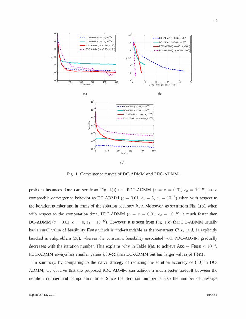
Fig. 1: Convergence curves of DC-ADMM and PDC-ADMM.
problem instances. One can see from Fig. 1(a) that PDC-ADMM (c = τ = 0.01, ǫ2 = 10−6) has a
comparable convergence behavior as DC-ADMM (c = 0.01, c1 = 5, ǫ1 = 10−6) when with respect to
the iteration number and in terms of the solution accuracyAcc. Moreover, as seen from Fig. 1(b), when
with respect to the computation time, PDC-ADMM (c = τ = 0.01, ǫ2 = 10−6) is much faster than
DC-ADMM (c = 0.01, c1 = 5, ǫ1 = 10−6). However, it is seen from Fig. 1(c) that DC-ADMM usually
has a small value of feasibilityFeas which is understandable as the constraintCixi di is explicitly
handled in subproblem (30); whereas the constraint feasibility associated with PDC-ADMM gradually
decreases with the iteration number. This explains why in Table I(a), to achieveAcc + Feas ≤ 10−4,
PDC-ADMM always has smaller values ofAcc than DC-ADMM but has larger values ofFeas.
In summary, by comparing to the naive strategy of reducing the solution accuracy of (30) in DC-
ADMM, we observe that the proposed PDC-ADMM can achieve a much better tradeoff between the
iteration number and computation time. Since the iterationnumber is also the number of message
September 12, 2014 DRAFT

18
0 100 200 300 400 500 600 70010
−6
10−5
10−4
10−3
10−2
10−1
100
Iteration
Acc
α=1, pe=0
α=0.7, pe=0
α=1, pe=0.1
α=0.7, pe=0.1
α=0.7, pe=0.5
(a)
0 100 200 300 400 500 600 70010
−5
10−4
10−3
10−2
10−1
100
Iteration
Fea
sibi
lity
α=1, pe=0
α=0.7, pe=0
α=1, pe=0.1
α=0.7, pe=0.1
α=0.7, pe=0.5
(b)
Fig. 2: Convergence curves of randomized PDC-ADMM.
exchanges between connecting agents, the results equivalently show that the proposed PDC-ADMM
achieves a better tradeoff between communication overheadand computational complexity.
In Table I(b), we present another set of simulation results for N = 50, K = 1, 000, L = 100, P = 500
andλ = 100. One can still observe that the proposed PDC-ADMM has a better tradeoff between the
iteration number and computation time compared to DC-ADMM.In particular, one can see that, for
DC-ADMM with ǫ1 reduced fromǫ1 = 10−6 to ǫ1 = 10−5, reduction of the computation time is limited
but the iteration number increased to a large number of 1173.
Example 2: In this example, we examine the convergence behavior of randomized PDC-ADMM
(Algorithm 3). It is set thatα , α1 = · · · = αN , i.e., all agents have the same active probability.
Note that, forα = 1 andpe = 0, randomized PDC-ADMM performs identically as the PDC-ADMMin
Algorithm 1. Figure 2 presents the convergence curves of randomized PDC-ADMM for different values
of α and pe and for the stopping condition beingAcc + Feas ≤ 10−4. The simulation setting and
problem instance are the same as that used for PDC-ADMM (c = τ = 0.05, ǫ2 = 10−5) in Fig. 1. One
can see from Fig. 2(a) that no matter whenα decreases to0.7 and/orpe increases to0.5, randomized
PDC-ADMM always exhibits consistent convergence behavior, though the convergence speed decreases
accordingly. We also observe from Fig. 2(a) thatAcc may oscillate in the first few iterations whenα < 1
andpe > 0. Interestingly, from Fig. 2(b), one can observe that the values ofα andpe do not affect the
convergence behavior of constraint feasibility much.
September 12, 2014 DRAFT

19
VI. CONCLUSIONS
In this paper, we have proposed two ADMM based distributed optimization methods, namely the PDC-
ADMM method (Algorithm 1) and the randomized PDC-ADMM method (Algorithm 3) for the polyhedra
constrained problem(P). In contrast to the existing DC-ADMM where each agent requires to solve a
polyhedra constrained subproblem at each iteration, agents in the proposed PDC-ADMM and randomized
PDC-ADMM methods deal with a subproblem with simple constraints only, thereby more efficiently
implementable than DC-ADMM. For both proposed PDC-ADMM andrandomized PDC-ADMM, we
have shown that they have a worst-caseO(1/k) convergence rate. The presented simulation results based
on the constrained LASSO problem in (2) have shown that the proposed PDC-ADMM method exhibits
a much lower computation time than DC-ADMM, although the required iteration number is larger. It
has been observed that the tradeoff between communication overhead and computational complexity of
PDC-ADMM is much better, especially when comparing to the naive strategy of reducing the subproblem
solution accuracy of DC-ADMM. It has been also shown that theproposed randomized PDC-ADMM
method can converge consistently in the presence of randomly ON/OFF agents and severely unreliable
links.
VII. A CKNOWLEDGEMENT
The author would like to thank Prof. Min Tao at the Nanjing University for her valuable discussions.
APPENDIX A
PROOF OFEQUATION (16)
It is easy to derive from (10) and (11) thattkij andski have close-form solutions as
tkij =yki + yk
j
2+
uk−1ij + vk−1
ij
2c, (A.1)
ski = zki +
wk−1i
τi, (A.2)
respectively. By substituting (A.1) into (14) and (15), respectively, followed by summing the two equa-
tions, one obtains
ukij + vk
ij = 0, ∀k, i, j. (A.3)
By (A.3), (A.1) reduces to
tkij =yki + yk
j
2∀k, i, j. (A.4)
On the other hand, it directly follows from (A.2) and (13) that wki = 0 andski = zk
i ∀i, k.
September 12, 2014 DRAFT

20
APPENDIX B
PROOF OFEQUATIONS (22) AND (23)
By (7) and (20), subproblem (17) can be explicitly written asa min-max problem as follows
(yki ,z
ki ) = argmin
yi,zi
maxxi∈Si,ri≥0
−fi(xi)−yTi (Eixi −
1Nq−pk−1
i )
+ c∑
j∈Ni‖yi −
yk−1
i +yk−1
j
2 ‖22
− zTi (Cixi + ri − di) +
τi2‖zi − zk−1
i ‖22
,
= argminyi,zi
maxxi∈Si,ri≥0
L(xi, ri,yi,zi) (A.5)
where
L(xi, ri,yi,zi) =−fi(xi)−c
4|Ni|
∥
∥
∥
∥
1c(Eixi −
1Nq)− 1
cpk−1i +
∑
j∈Ni(yk−1
i + yk−1j )
∥
∥
∥
∥
2
2
−1
2τi
∥
∥
∥
∥
Cixi + ri − di + τizk−1i
∥
∥
∥
∥
2
2
+ (c|Ni|)
∥
∥
∥
∥
yi −1
2|Ni|[∑
j∈Ni(yk−1
i + yk−1j )− 1
cpk−1i + 1
c(Eix
ki −
1Nq)]
∥
∥
∥
∥
2
2
+τi2
∥
∥
∥
∥
zi − [zk−1i +
1
τi(Cix
ki + rki − di)]
∥
∥
∥
∥
2
2
. (A.6)
Notice that L(xi, ri,yi,zi) is (strongly) convex with respect to(yi,zi) given any (xi, ri) and is
concave with respect to(xi, ri) given any(yi,zi). Therefore, the minimax theorem [27, Proposition
2.6.2] can be applied so that saddle point exists for (A.5) and it is equivalent to its max-min counterpart
(xki , r
ki ) , arg max
xi∈Si,ri≥0
minyi,zi
L(xi, ri,yi,zi). (A.7)
Let (yki ,z
ki ) and (xk
i , rki ) be a pair of saddle point of (A.5) and (A.7). Then, given(xk
i , rki ), (y
ki ,z
ki )
is the unique inner minimizer of (A.7), which, from (A.6), can be readily obtained as the closed-form
solutions in (22a) and (22b), respectively. By substituting (22a) and (22b) into (A.7),(xki , r
ki ) can be
obtain by subproblem (23).
We remark here that if one removes the dummy constraintzi = si from (8) and the augmented term∑N
i=1τi2 ‖zi − si‖
22 from (9), then the corresponding subproblem (17) reduces to
(yki ,z
ki ) = argmin
yi,zi
maxxi∈Si,ri≥0
−fi(xi)−yTi (Eixi −
1Nq−pk−1
i )
+ c∑
j∈Ni‖yi −
yk−1
i +yk−1
j
2 ‖22 − zTi (Cixi + ri − di)
. (A.8)
September 12, 2014 DRAFT

21
Note that (A.8) is no longer strongly convex with respect tozi as the termτi2‖zi − zk−1
i ‖22 is absent.
After applying the minmax theorem to (A.8):
(xki , r
ki ) , arg max
xi∈Si,ri≥0
minyi,zi
−fi(xi)−yTi (Eixi −
1Nq−pk−1
i )
+ c∑
j∈Ni
(
‖yi −yk−1
i +yk−1
j
2 ‖22 − zTi (Cixi + ri − di)
,
one can see that, to have a bounded optimal value for the innerminimization problem, it must hold
Cixi + ri − di = 0, and thuszi appears redundant. Moreover, one can show that the inner optimal y is
yki = 1
2|Ni|(∑
j∈Ni(yk−1
i + yk−1j )− 1
cpk−1i
+ 1c(Eix
ki −
1Nq))
, (A.9)
where
(xki , r
ki ) = arg max
xi∈Si,ri≥0
fi(xi) +c
4|Ni|
∥
∥
1c(Eixi −
1Nq)
− 1cpki +
∑
j∈Ni(yk−1
i + yk−1j )
∥
∥
2
2
s.t. Cixi + ri = di. (A.10)
The variableri also appears redundant and can be removed from (A.10). The resultant steps of (A.9),
(A.10) and (21) are the DC-ADMM method in [19] (see Algorithm2).
APPENDIX C
PROOF OFTHEOREM 1
Let us equivalently write (26) to (29) as follows:∀i ∈ V,
ukij = uk−1
ij + c(yk−1
i −yk−1
j
2 ) ∀j ∈ Ni, (A.11)
vkji = vk−1
ji + c(yk−1
i −yk−1
j
2 ) ∀j ∈ Ni, (A.12)
(xki , r
ki )=arg min
xi∈Si,ri0
fi(xi)+1
4c|Ni|
∥
∥(Eixi −1Nq)
−∑
j∈Ni(uk
ij + vkji) + c
∑
j∈Ni(yk−1
i + yk−1j )
∥
∥
2
2
+ 12τi
‖Cixi + ri − di + τizk−1i ‖22
, (A.13)
September 12, 2014 DRAFT

22
yki = 1
2c|Ni|(
c∑
j∈Ni(yk−1
i + yk−1j )−
∑
j∈Ni(uk
ij + vkji) + (Eix
ki −
1Nq))
, (A.14)
zki = zk−1
i +1
τi(Cix
ki + rki − di). (A.15)
Notice that we have recovereduk−1ij ,vk−1
ji from pk−1i according to (18), (19), and (21). Besides, the
update orders of(uij,vji) and (xi, ri,yi,zi) are reversed here for ease of the analysis.
According to [14, Lemma 4.1], the optimality condition of (A.13) with respect toxi is given by:
∀xi ∈ Si,
0 ≥ fi(xki )− fi(xi) +
12c|Ni|
(
c∑
j∈Ni(yk−1
i + yk−1j )
−∑
j∈Ni(uk
ij + vkji) + (Eix
ki −
1Nq))T
Ei(xki − xi)
+ 1τi(Cix
ki + rki − di + τiz
k−1i )TCi(x
ki − xi)
= fi(xki )− fi(xi) + (yk
i )TEi(x
ki − xi)
+ (zki )
TCi(xki − xi), (A.16)
where the equality is obtained by using (A.14) and (A.15). Analogously, the optimality condition of
(A.13) with respect tori is given by,∀ri 0,
0 ≥1
τi(Cix
ki + rki − di + τiz
k−1i )(rki − ri)
= (zki )
T (rki − ri), (A.17)
where the equality is owing to (A.15). By summing (A.16) and (A.17), one obtains
0 ≥ fi(xki )− fi(xi) + (yk
i )TEi(x
ki − xi)
+ (zki )
T (Cixki + rki −Cixi − ri) ∀xi ∈ Si, ri 0. (A.18)
By letting xi = x⋆i andri = r⋆i for all i ∈ V in (A.18), where(x⋆
i , r⋆i )
Ni=1 denotes the optimal solution
to problem (5), we have the following chain from (A.18)
0 ≥ fi(xki )− fi(x
⋆i ) + (yk
i )TEi(x
ki − x⋆
i )
+ (zki )
T (Cixki + rki −Cix
⋆i − r⋆i )
= fi(xki )− fi(x
⋆i ) + (yk
i )TEi(x
ki − x⋆
i ) + (zki )
T (Cixki + rki − di)
= fi(xki ) + yT (Eix
ki − q/N) + zT
i (Cixki + rki − di)
− fi(x⋆i )− yT (Eix
⋆i − q/N) + (yk
i − y)TEi(xki − x⋆
i )+(zki − zi)
T (Cixki + rki − di)
(A.19)
September 12, 2014 DRAFT

23
= fi(xki ) + yT (Eix
ki − q/N) + zT
i (Cixki + rki − di)
− fi(x⋆i )− yT (Eix
⋆i − q/N) + (yk
i − y)TEi(xki − x⋆
i )
+τi(zki − zi)
T (zki − zk−1
i ), (A.20)
where the first equality is due to the factCix⋆i +r⋆i = di; the second equality is obtained by adding and
subtracting both termsyTEi(x
ki −x⋆
i ) andzTi (Cix
ki + rki − di) for arbitraryy andzi; the last equality
is due to (A.15).
On the other hand, note that (A.14) can be expressed as
0 = 2c|Ni|yki − c
∑
j∈Ni(yk−1
i + yk−1j )
− (Eixki − q/N) +
∑
j∈Ni(uk
ij + vkji)
= 2c∑
j∈Ni(yk
i −yk
i +ykj
2 ) +∑
j∈Ni(uk
ij + vkji)
+ c∑
j∈Ni(yk
i + ykj − yk−1
i − yk−1j )− (Eix
ki − q/N)
=∑
j∈Ni(uk+1
ij + vk+1ji )− (Eix
ki − q/N)
+ c∑
j∈Ni(yk
i + ykj − yk−1
i − yk−1j ), (A.21)
where the last equality is obtained by applying (A.11) and (A.12). Furthermore, let(y⋆i ,z
⋆i )
Ni=1 be an
optimal solution to problem (8), and denote(u⋆ij, v
⋆ij) be an optimal dual solution of (8). Then,
according to the Karush-Kuhn-Tucker (KKT) condition [31],we have
∂yiϕ(y⋆
i ,z⋆i ) + q/N +
∑
j∈Ni(u⋆
ij + v⋆ji) = 0, (A.22)
where∂yiϕ(y⋆
i ,z⋆i ) denotes a subgradient ofϕ with respect toyi at point(y⋆
i ,z⋆i ). Sincey⋆ , y⋆
i = · · · =
y⋆N under Assumption 1,(x⋆
i , r⋆i )
Ni=1 and(y⋆, z⋆
i Ni=1) form a pair of primal-dual solution to problem (5)
under Assumption 2,(x⋆i , r
⋆i ) is optimal to (7) given(y,zi) = (y⋆
i ,z⋆i ), and thus∂yi
ϕ(y⋆i ,z
⋆i ) = −Eix
⋆i
[37], which and (A.22) give rise to
Eix⋆i − q/N −
∑
j∈Ni(u⋆
ij + v⋆ji) = 0. (A.23)
By combing (A.21) and (A.23) followed by multiplying(yki −y) on both sides of the resultant equation,
one obtains
(yki − y)TEi(x
ki − x⋆
i )
= c∑
j∈Ni(yk
i + ykj − yk−1
i − yk−1j )T (yk
i − y)
+∑
j∈Ni(uk+1
ij + vk+1ji − u⋆
ij − v⋆ji)
T (yki − y). (A.24)
September 12, 2014 DRAFT

24
By further substituting (A.24) into (A.19) and summing fori = 1, . . . , N , one obtains that
F (xk) + yT (∑N
i=1Eixki − q) +
∑Ni=1 z
Ti (Cix
ki + rki − di)
− F (x⋆) +∑N
i=1 τi(zki − zi)
T (zki − zk−1
i )
+ c∑N
i=1
∑
j∈Ni(yk
i + ykj − yk−1
i − yk−1j )T (yk
i − y)
+∑N
i=1
∑
j∈Ni(uk+1
ij + vk+1ji − u⋆
ij − v⋆ji)
T (yki − y)
≤ 0, (A.25)
for arbitraryy andz1, . . . ,zN , wherexk = [(xk1)
T , . . . , (xkN )T ]T .
By following the same idea as in [19, Eqn. (A.16)], one can show that
c∑N
i=1
∑
j∈Ni(yk
i + ykj − yk−1
i − yk−1j )T (yk
i − y)
= c(yk − yk−1)TQ(yk − y), (A.26)
whereyk = [(yk1 )
T , . . . , (ykN )T ]T , y , 1N ⊗ y andQ , (D + W ) ⊗ IL 0 (see [19, Remark 1]).
Moreover, according to [19, Eqn. (A.15)], it can be shown that
∑Ni=1
∑
j∈Ni(uk+1
ij + vk+1ji − u⋆
ij − v⋆ji)
T (yki − y)
= 2c(uk+1 − u⋆)T (uk+1 − uk), (A.27)
whereuk (u⋆) is a vector that stacksukij (u⋆
ij) for all j ∈ Ni and i ∈ V. As a result, (A.25) can be
expressed as
F (xk) + yT (∑N
i=1Eixki − q) +
∑Ni=1 z
Ti (Cix
ki + rki − di)
− F (x⋆) + (zk − z)TΓ(zk − zk−1)
+ c(yk − yk−1)TQ(yk − y)
+ 2c(uk+1 − u⋆)T (uk+1 − uk) ≤ 0, (A.28)
wherezk = [(zk1 )
T , . . . , (zkN )T ]T , z = [zT
1 , . . . ,zTN ]T andΓ , diagτ1, . . . , τN. By applying the fact
of
(ak − ak−1)TA(ak − a⋆)
≥1
2‖ak − a⋆‖2A −
1
2‖ak−1 − a⋆‖2A (A.29)
September 12, 2014 DRAFT

25
for any sequenceak and matrixA 0, to (A.28), we obtain
F (xk) + yT (∑N
i=1Eixki − q) +
∑Ni=1 z
Ti (Cix
ki + rki − di)
− F (x⋆) + 12(‖z
k − z‖2Γ− ‖zk−1 − z‖2
Γ)
+ c2 (‖y
k − y‖2Q − ‖yk−1 − y‖2Q)
+ 1c(‖uk+1 − u⋆‖22 − ‖uk − u⋆‖22) ≤ 0. (A.30)
Summing (A.30) fork = 1, . . . ,M, and taking the average gives rise to
0 ≥ 1M
∑Mk=1[F (xk) + yT (
∑Ni=1 Eix
ki − q)
+∑N
i=1 zTi (Cix
ki + rki − di)]− F (x⋆)
+ 12M (‖zM − z‖2
Γ− ‖z0 − z‖2
Γ)
+ c2M (‖yM − y‖2Q − ‖y0 − y‖2Q)
+ 1c(‖uM+1 − u⋆‖22 − ‖u1 − u⋆‖22)
≥ F (xM ) + yT (∑N
i=1 EixMi − q)
+∑N
i=1 zTi (Cix
Mi + rMi − di)− F (x⋆)− 1
2M ‖z0 − z‖2Γ
− c2M ‖y0 − y‖2Q − 1
cM‖u1 − u⋆‖22, (A.31)
where xMi , 1
M
∑Mk=1 x
ki , rMi , 1
M
∑Mk=1 r
ki , and the last inequality is owing to the convexity ofF
(Assumption 2).
Let y = y⋆ +∑
Ni=1
EixMi −q
‖∑N
i=1EixM
i −q‖2
andzi = z⋆i +
CixMi +rM
i −di
‖CixMi +rM
i −di‖2
∀i ∈ V, in (A.31). Moreover, note that
F (xM ) + (y⋆)T (∑N
i=1 EixMi − q)
+∑N
i=1(z⋆i )
T (CixMi + rMi − di)− F (x⋆) ≥ 0, (A.32)
according to the duality theory [31]. Thus, we obtain that
‖∑N
i=1EixMi − q‖2 +
∑Ni=1 ‖Cix
Mi + rMi − di‖2
≤1
2Mmax
‖a‖2≤√N
‖z0 − (z⋆ + a)‖2Γ +1
cM‖u1 − u⋆‖22
+c
2Mmax
‖a‖2≤1‖y0 − 1N ⊗ (y⋆ + a)‖2Q ,
C1
M. (A.33)
September 12, 2014 DRAFT

26
On the other hand, lety = y⋆ andzi = z⋆i ∀i ∈ V, in (A.31). Then, we have that
1
2M‖z0 − z⋆‖2Γ +
c
2M‖y0 − 1N ⊗ y⋆‖2Q +
1
cM‖u1 − u⋆‖22
≥ F (xM ) + (y⋆)T (∑N
i=1EixMi − q)
+∑N
i=1(z⋆i )
T (CixMi + rMi − di)− F (x⋆)
≥ |F (xM )− F (x⋆)| − δ(‖∑N
i=1EixMi − q‖2
+∑N
i=1 ‖CixMi + rMi − di‖2), (A.34)
whereδ , max‖y⋆‖2, ‖z⋆1‖2, . . . , ‖z
⋆N‖2. Using (A.33), (A.34) implies that
|F (xM )− F (x⋆)| ≤δC1 + C2
M, (A.35)
whereC2 ,12‖z
0 − z⋆‖2Γ+ c
2‖y0 − 1N ⊗ y⋆‖2Q + 1
c‖u1 −u⋆‖22. After summing (A.33) and (A.35), one
obtains (43).
APPENDIX D
PROOF OFTHEOREM 2
The proof is based on the “full iterates” assuming that all agents and all edges are active at iteration
k. Specifically, the full iterates for iterationk are
(xki , r
ki )=arg min
xi∈Si,ri0
fi(xi)+c
4|Ni|
∥
∥
1c(Eixi
− 1Nq) − 1
c
∑
j∈Ni(uk−1
ij + vk−1ji ) + 2
∑
j∈Nitk−1ij
+ 12τi
‖Cixi + ri − di + τizk−1i ‖22
∀i ∈ V, (A.36)
yki = 1
2|Ni|(
2∑
j∈Nitk−1ij − 1
c
∑
j∈Ni(uk−1
ij + vk−1ji )
+ 1c(Eix
ki −
1Nq))
∀i ∈ V, (A.37)
zki = zk−1
i + 1τi(Cix
ki + rki − di) ∀i ∈ V, (A.38)
tkij =yki + yk
j
2∀j ∈ Ni, i ∈ V, (A.39)
ukij = uk−1
ij + c(yki − tkij) ∀j ∈ Ni, i ∈ V, (A.40)
vkji = vk−1
ji + c(yki − tkij) ∀j ∈ Ni, i ∈ V. (A.41)
September 12, 2014 DRAFT
27
It is worthwhile to note that
(xki , r
ki ) = (xk
i , rki ), yk
i = yki , zk
i = zki ∀i ∈ Ωk, (A.42)
tkij = tkij, ukij = uk
ij , vkji = vk
ji ∀(i, j) ∈ Ψk. (A.43)
Let us consider the optimality condition of (A.36). Following similar steps as in (A.16) to (A.19), one
can have that
0 ≥ fi(xki ) + yT (Eix
ki − q/N) + zT
i (Cixki + rki − di)
− fi(x⋆i )− yT (Eix
⋆i − q/N) + (yk
i − y)TEi(xki − x⋆
i )
+τi(zki − zi)
T (zki − zk−1
i ). (A.44)
Besides, note that (A.37) can be expressed as
0 = 2c|Ni|yki − 2c
∑
j∈Nitk−1ij
+∑
j∈Ni(uk−1
ij + vk−1ji )− (Eix
ki − q/N)
= 2c∑
j∈Ni(yk
i − tkij) +∑
j∈Ni(uk−1
ij + vk−1ji )
+ 2c∑
j∈Ni(tkij − tk−1
ij )− (Eixki − q/N)
=∑
j∈Ni(uk
ij + vkji) + 2c
∑
j∈Ni(tkij − tk−1
ij )
− (Eixki − q/N)
= −Eix⋆i + q/N +
∑
j∈Ni(u⋆
ij + v⋆ji), (A.45)
where the third equality is due to (A.40) and (A.41), and the last equality is obtained by invoking (A.23).
By multiplying (yki − y) with the last two terms in (A.45), we obtain
(yki − y)TEi(x
ki − x⋆
i ) = 2c∑
j∈Ni(tkij − tk−1
ij )T (yki − y)
+∑
j∈Ni(uk
ij + vkji − u⋆
ij − v⋆ji)
T (yki − y). (A.46)
By substituting (A.46) into (A.44) and summing the equations for i = 1, . . . , N , one obtains
F (xk) + yT (∑N
i=1Eixki − q) +
∑Ni=1 z
Ti (Cix
ki + rki − di)
− F (x⋆) +∑N
i=1 τi(zki − zi)
T (zki − zk−1
i )
+ 2c∑N
i=1
∑
j∈Ni(tkij − tk−1
ij )T (yki − y)
+∑N
i=1
∑
j∈Ni(uk
ij + vkji − u⋆
ij − v⋆ji)
T (yki − y) ≤ 0. (A.47)
September 12, 2014 DRAFT

28
Also note that
2c∑N
i=1
∑
j∈Ni(tkij − tk−1
ij )T (yki − y)
= c∑N
i=1
∑
j∈Ni(tkij − tk−1
ij )T (yki − y)
+ c∑N
i=1
∑
j∈Ni(tkji − tk−1
ji )T (ykj − y)
= c∑N
i=1
∑
j∈Ni(tkij − tk−1
ij )T (yki + yk
j − 2y)
= 2c∑N
i=1
∑
j∈Ni(tkij − tk−1
ij )T (tkij − y)
= 2c(tk − tk−1)T (tk − 1|E| ⊗ y)
≥ c‖tk − 1|E| ⊗ y‖22 − c‖tk−1 − 1|E| ⊗ y‖22, (A.48)
where the first equality is obtained by the fact that, for anyαij,N∑
i=1
∑
j∈Ni
αij =
N∑
i=1
N∑
j=1
[W ]i,jαij
=
N∑
i=1
N∑
j=1
[W ]i,jαji =
N∑
i=1
∑
j∈Ni
αji, (A.49)
owing to the symmetric property ofW ; the second equality is due to the fact oftkij = tkji andtkij = tkji
for all i, j andk; the third equality is from (A.39); the fourth equality is bydefiningtk (tk−1) as a vector
that stackstkij (tk−1ij ) for all j ∈ Ni, i ∈ V; and the last inequality is obtained by applying (A.29).
Then, similar to the derivations from (A.25) to (A.30), one can deduce from (A.47) and (A.48) that
L(xk, rk,y,z) − L(x⋆, r⋆,y,z)
+ 12(‖z
k − z‖2Γ− ‖zk−1 − z‖2
Γ)
+ c(‖tk − 1|E| ⊗ y‖22 − ‖tk−1 − 1|E| ⊗ y‖22)
+ 1c(‖uk − u⋆‖22 − ‖uk−1 − u⋆‖22) ≤ 0, (A.50)
where
L(xk, rk,y,z) , F (xk) + yT (∑N
i=1 Eixki − q)
+∑N
i=1 zTi (Cix
ki + rki − di). (A.51)
To connect the full iterates with the instantaneous iterates, let us define a weighed Lagrangian as
L(xk, rk,y,z) ,∑N
i=11αifi(x
ki ) + yT
∑Ni=1
1αi(Eix
ki − q)
+∑N
i=11αizTi (Cix
ki + rki − di). (A.52)
September 12, 2014 DRAFT
29
Moreover, letJk−1 , xℓ, rℓ,uℓ,Ψi,Ωi, ℓ = k − 1, . . . , 0 be the set of historical events up to iteration
k − 1. By (A.42) and (39), the conditional expectation ofL(xk, rk,y,z) can be shown as
E[L(xk, rk,y,z)|Jk−1] = L(xk, rk,y,z)
+ L(xk−1, rk−1,y,z) − L(xk−1, rk−1,y,z)
≤ L(xk−1, rk−1,y,z)− L(xk−1, rk−1,y,z)
− L(x⋆, r⋆,y,z)− 12‖z
k − z‖2Γ+ 1
2‖zk−1 − z‖2
Γ)
− c‖tk − 1|E| ⊗ y‖22 + c‖tk−1 − 1|E| ⊗ y‖22
− 1c‖uk − u⋆‖22 +
1c‖uk−1 − u⋆‖22, (A.53)
where the last inequality is due to (A.50). Furthermore, define
Gz(zk,z) ,
∑Ni=1
1αi‖zk
i − z‖2Γ, (A.54)
Gt(tk,y) ,
∑Ni=1
∑
j∈Ni
1βij
‖tkij − 1|E| ⊗ y‖22, (A.55)
Gu(uk,u⋆) ,
∑Ni=1
∑
j∈Ni
1βij
‖ukij − u⋆
ij‖22. (A.56)
Then, by (A.42), (A.43) and (39), one can show that
E[Gz(zk,z)|Jk−1] = Gz(z
k−1,z)
+ ‖zk − z‖2Γ − ‖zk−1 − z‖2Γ, (A.57)
E[Gt(tk,y)|Jk−1] = Gt(t
k−1,y)
+ ‖tk − 1|E| ⊗ y‖22 − ‖tk−1 − 1|E| ⊗ y‖22, (A.58)
E[Gu(uk,u⋆)|Jk−1] = Gu(u
k−1,u⋆),
+ ‖uk − u⋆‖22 − ‖uk−1 − u⋆‖22. (A.59)
By substituting (A.57), (A.58) and (A.59) into (A.53) followed by taking the expectation with respect to
Jk−1, one obtains
E[L(xk−1, rk−1,y,z)] − L(x⋆, r⋆,y,z)
≤ E[L(xk−1, rk−1,y,z)]− E[L(xk, rk,y,z)]
+1
2E[Gz(z
k−1,z)] −1
2E[Gz(z
k,z)] + cE[Gt(tk−1,y)]
− cE[Gt(tk,y)] +
1
cE[Gu(u
k−1,u⋆)]−1
cE[Gu(u
k,u⋆)].
September 12, 2014 DRAFT

30
Upon summing the above equation fromk = 1, . . . ,M , and taking the average, we can obtain the
following bound
0 ≥ E[ 1M
∑Mk=1L(x
k−1, rk−1,y,z)] − L(x⋆, r⋆,y,z)
+ 1M(E[L(xM , rM ,y,z)] − E[L(x0, r0,y,z)])
− 1cM
E[Gu(u0,u⋆)]− c
ME[Gt(t
0,y)]− 12ME[Gz(z
0,z)]
≥ E[L(xM , rM ,y,z)] − L(x⋆, r⋆,y,z)
+ 1M(E[L(xM , rM ,y,z)] − E[L(x0, r0,y,z)])
− 1cM
E[Gu(u0,u⋆)]− c
ME[Gt(t
0,y)]− 12ME[Gz(z
0,z)]. (A.60)
Similar to (A.32) and (A.33), by lettingy = y⋆ +E[∑
N
i=1Eix
Mi −q]
‖E[∑N
i=1EixM
i −q]‖2
andzi = z⋆i + E[Cix
Mi +rM
i −di]‖E[Cix
Mi +rM
i −di]‖2
∀i ∈ V, one can bound the feasibility of(xM , rM ) from (A.60) as
‖E[∑N
i=1EixMi − q]‖2
+∑N
i=1 ‖E[CixMi + rMi − di]‖2 ≤
C1
M, (A.61)
where
C1 , max‖a1‖2≤1,‖a2‖2≤
√N
E[L(x0, r0,y⋆ + a1,z⋆ + a2)]
− E[L(xM , rM ,y⋆ + a1,z⋆ + a2)]
+ cE[Gt(t0,y⋆ + a1)] +
1
2E[Gz(z
0,z⋆ + a2)]
+1
cE[Gu(u
0,u⋆)]. (A.62)
Also similar to (A.34) and (A.35), by lettingy = y⋆ andz = z⋆, one can bound the expected objective
value as
|E[F (xM )− F (x⋆)]| ≤δC1 + C2
M, (A.63)
whereδ , max‖y⋆‖2, ‖z⋆1‖2, . . . , ‖z
⋆N‖2 and
C2 , E[L(x0, r0,y⋆,z⋆)]− E[L(xM , rM ,y⋆,z⋆)]
+ cE[Gt(t0,y⋆ + a1)] +
1
2E[Gz(z
0,z⋆ + a2)]
+1
cE[Gu(u
0,u⋆)]. (A.64)
The proof is complete by adding (A.61) and (A.63).
September 12, 2014 DRAFT
31
REFERENCES
[1] B. Yang and M. Johansson, “Distributed optimization andgames: A tutorial overview,” Chapter 4 ofNetworked Control
Systems, A. Bemporad, M. Heemels and M. Johansson (eds.), LNCIS 406,Springer-Verlag, 2010.
[2] V. Lesser, C. Ortiz, and M. Tambe,Distributed Sensor Networks: A Multiagent Perspective. Kluwer Academic Publishers,
2003.
[3] I. Foster, Y. Zhao, I. Raicu, and S. Lu, “Cloud computing and grid computing 360-degree compared,” inProc. Grid
Computing Environments Workshop, Austin, TX, USA, Nov. 12-16, 2008, pp. 1–10.
[4] R. Bekkerman, M. Bilenko, and J. Langford,Scaling up Machine Learning- Parallel and Distributed Approaches.
Cambridge University Press, 2012.
[5] S. Chen, D. Donoho, and M. Saunders, “Atomic decomposition by basis pursuit,”SIAM J. Sci. Comput., vol. 20, no. 1,
pp. 33–61, 1998.
[6] T. Hastie, R. Tibshirani, and J. Friedman,The Elements of Statistical Learning: Data Mining, Inference, and Prediction.
New York, NY, USA: Springer-Verlag, 2001.
[7] M. Alizadeh, X. Li, Z. Wang, A. Scaglione, and R. Melton, “Demand side management in the smart grid: Information
processing for the power switch,”IEEE Signal Process. Mag., vol. 59, no. 5, pp. 55–67, Sept. 2012.
[8] D. P. Bertsekas,Network Optimization : Contribuous and Discrete Models. Athena Scientific, 1998.
[9] C. Shen, T.-H. Chang, K.-Y. Wang, Z. Qiu, and C.-Y. Chi, “Distributed robust multicell coordianted beamforming with
imperfect CSI: An ADMM approach,”IEEE Trans. Signal Process., vol. 60, no. 6, pp. 2988–3003, 2012.
[10] A. Nedic and A. Ozdaglar, “Distributed subgradient methods for multi-agent optimization,”IEEE Trans. Auto. Control,
vol. 54, no. 1, pp. 48–61, Jan. 2009.
[11] M. Zhu and S. Martınez, “On distributed convex optimization under inequality and equality constraints,”IEEE Trans. Auto.
Control, vol. 57, no. 1, pp. 151–164, Jan. 2012.
[12] J. Chen and A. H. Sayed, “Diffusion adaption strategiesfor distributed optimization and learning networks,”IEEE. Trans.
Signal Process., vol. 60, no. 8, pp. 4289–4305, Aug. 2012.
[13] T.-H. Chang, A. Nedic, and A. Scaglione, “Distributedconstrained optimization by consensus-based primal-dualperturba-
tion method,”IEEE. Trans. Auto. Control., vol. 59, no. 6, pp. 1524–1538, June 2014.
[14] D. P. Bertsekas and J. N. Tsitsiklis,Parallel and distributed computation: Numerical methods. Upper Saddle River, NJ,
USA: Prentice-Hall, Inc., 1989.
[15] S. Boyd, N. Parikh, E. Chu, B. Peleato, and J. Eckstein, “Distributed optimization and statistical learning via thealternating
direction method of multipliers,”Foundations and Trends in Machine Learning, vol. 3, no. 1, pp. 1–122, 2011.
[16] G. Mateos, J. A. Bazerque, and G. B. Giannakis, “Distributed sparse linear regression,”IEEE Trans. Signal Process.,
vol. 58, no. 10, pp. 5262–5276, Dec. 2010.
[17] J. F. C. Mota, J. M. F. Xavier, P. M. Q. Aguiar, and M. Puschel, “Distributed basis pursuit,”IEEE. Trans. Signal Process.,
vol. 60, no. 4, pp. 1942–1956, April 2012.
[18] ——, “D-ADMM: A communication-efficient distributed algorithm for separable optimization,”IEEE. Trans. Signal
Process., vol. 60, no. 10, pp. 2718–2723, May 2013.
[19] T.-H. Chang, M. Hong, and X. Wang, “Multi-agent distributed optimization via inexact consensus ADMM,” submitted to
IEEE Trans. Signal Process.;available on arxiv.org.
[20] W. Shi, Q. Ling, K. Yuan, G. Wu, and W. Yin, “On the linear convergence of the ADMM in decentralized consensus
optimization,” IEEE Trans. Signal Process., vol. 62, no. 7, pp. 1750–1761, April 2014.
September 12, 2014 DRAFT

32
[21] E. Wei and A. Ozdaglar, “On theO(1/K) convergence of asynchronous distributed alternating direction method of
multipliers,” available on arxiv.org.
[22] D. P. Bertsekas,Nonlinear Programming: 2nd Ed.Cambridge, Massachusetts: Athena Scientific, 2003.
[23] T.-H. Chang, M. Alizadeh, and A. Scaglione, “Coordinated home energy management for real-time power balancing,” in
Proc. IEEE PES General Meeting, San Diego, CA, July 22-26, 2012, pp. 1–8.
[24] Y. Zhang and G. B. Giannakis, “Efficient decentralized economic dispatch for microgrids with wind power integration,”
available on arxiv.org.
[25] S. S. Ram, A. Nedic, and V. V. Veeravalli, “A new class ofdistributed optimization algorithm: Application of regression
of distributed data,”Optimization Methods and Software, vol. 27, no. 1, pp. 71–88, 2012.
[26] G. M. James, C. Paulson, and P. Rusmevichientong, “The constrained Lasso,” working paper, available on http://www-bcf.
usc.edu/∼rusmevic/.
[27] D. P. Bertsekas, A. Nedic, and A. E. Ozdaglar,Convex analysis and optimization. Cambridge, Massachusetts: Athena
Scientific, 2003.
[28] L. Grippo and M. Sciandrone, “On the convergence of the block nonlinear gauss-seidel method under convex constraints,”
Operation research letter, vol. 26, pp. 127–136, 2000.
[29] M. Razaviyayn, M. Hong, and Z.-Q. Luo, “A unified convergence analysis of block successive minimization methods for
nonsmooth optimization,”SIAM J. OPtim., vol. 23, no. 2, pp. 1126–1153, 2013.
[30] A. Beck and M. Teboulle, “A fast iterative shrinkage-thresholding algorithm for linear inverse problems,”SIAM J. Imaging
Sci., vol. 2, no. 1, pp. 183–202, 2009.
[31] S. Boyd and L. Vandenberghe,Convex Optimization. Cambridge, UK: Cambridge University Press, 2004.
[32] M. Hong, T.-H. Chang, X. Wang, M. Razaviyayn, S. Ma, and Z.-Q. Luo, “A block successive upper bound minimization
method of multipliers for linearly constrained convex optimization,” submittd toSIAM J. Opt.available on arxiv.org.
[33] Y. Nesterov, “Smooth minimization of nonsmooth functions,” Math. Program., vol. 103, no. 1, pp. 127–152, 2005.
[34] P. L. Combettes and J.-C. Pesquet, “Proximal splittingmethods in signal processing,” available on arxiv.org.
[35] M. Grant and S. Boyd, “CVX: Matlab software for disciplined convex programming, version 1.21,” http://cvxr.com/cvx,
Apr. 2011.
[36] M. E. Yildiz and A. Scaglione, “Coding with side information for rate-constrained consensus,”IEEE Trans. Signal Process.,
vol. 56, no. 8, pp. 3753–3764, 2008.
[37] S. Boyd and A. Mutapcic, “Subgradient methods,” avaliable at www.stanford.edu/class/ee392o/subgradmethod.pdf.
September 12, 2014 DRAFT
Recommended


![Overlapping Schwarz Decomposition for Nonlinear Optimal ... · [17], and Jacobi/Gauss-Seidel methods [18], [19]. Lagrangian dual decomposition, ADMM, and dual dynamic programming](https://img.pdfslide.us/doc/110x75/5f20426a361a060b480a45b0/overlapping-schwarz-decomposition-for-nonlinear-optimal-17-and-jacobigauss-seidel.jpg)