1 Multi-Agent Distributed Optimization via Inexact ... · PDF fileMulti-Agent Distributed Optimization via Inexact Consensus ADMM ... and these variables are coupled together through

arX

iv:1

402.

6065

v1 [

cs.S

Y]

25 F

eb 2

014

1

Multi-Agent Distributed Optimization viaInexact Consensus ADMM

Tsung-Hui Chang⋆, Mingyi Hong† and Xiangfeng Wang‡

Abstract

Multi-agent distributed consensus optimization problemsarise in many signal processing applications.Recently, the alternating direction method of multipliers(ADMM) has been used for solving this familyof problems. ADMM based distributed optimization method isshown to have faster convergence ratecompared with classic methods based on consensus subgradient, but can be computationally expensive,especially for problems with complicated structures or large dimensions. In this paper, we propose low-complexity algorithms that can reduce the overall computational cost of consensus ADMM by an orderof magnitude for certain large-scale problems. Central to the proposed algorithms is the use of an inexactstep for each ADMM update, which enables the agents to perform cheap computation at each iteration.Our convergence analyses show that the proposed methods canconverge well under mild conditions.Numerical results show that the proposed algorithms offer considerably lower computational complexityat the expense of extra communication overhead, demonstrating potential for certain big data scenarioswhere communication between agents can be implemented cheaply.

Keywords− Distributed optimization, ADMM, Consensus

EDICS: OPT-DOPT, MLR-DIST, NET-DISP, SPC-APPL.

The work of Tsung-Hui Chang is supported by National ScienceCouncil, Taiwan (R.O.C.), under Grant NSC 102-2221-E-011-005-MY3. The work of Xiangfeng Wang is supported by Doctoral Fund of the Ministry of Education, China,No.20110091110004. Part of this work was submitted to IEEE ICASSP 2014.

⋆Tsung-Hui Chang is the corresponding author. Address: Department of Electronic and Computer Engineering, NationalTaiwan University of Science and Technology, Taipei 10607,Taiwan, (R.O.C.). E-mail: [email protected].

†Mingyi Hong is with Department of Electrical and Computer Engineering, University of Minnesota, Minneapolis, MN 55455,USA, E-mail: [email protected]

‡Xiangfeng Wang is with Department of Mathematics, Nanjing University, Nanjing 210093, P. R. China, E-mail:[email protected]

March 10, 2018 DRAFT

http://arxiv.org/abs/1402.6065v1

2

I. INTRODUCTION

We consider a network with multiple agents, for example a sensor network with distributed sensor

nodes, a data cloud network with distributed database servers, a communication network with distributed

base stations (mobile users) or even a computer system with distributed microprocessors. We assume

that the network consists ofN agents who collaborate with each other to accomplish certain tasks. For

example, distributed database servers may cooperate for data mining or for parameter learning in order

to fully exploit the data collected from individual servers[1]. Another example arises from big data

applications [2], where a computation task may be executed by collaborative distributed microprocessors

with individual memories and storage spaces [3], [4]. Many of the distributed optimization tasks, such

as those described above, can be cast as a generic optimization problem of the following form

(P1) minx∈X

N∑

i=1

φi(x) (1)

wherex ∈ RK is the decision variable,X ⊆ R

K is the feasible set ofx, andφi : RK → R is the cost

function associated with agenti. Here the functionφi is composed of a smooth componentfi and a

non-smooth componentgi, i.e.,

φi(x) = fi(Aix) + gi(x),

whereAi ∈ RM×K is some data matrix not necessarily of full rank. Such model is common in practice:

the smooth component usually represents the cost function to be minimized, while the non-smooth

component is often used for regularization purposes [5].

In the setting of distributed optimization, it is commonly assumed that each agenti only has knowledge

about the local informationfi, gi andAi. The challenge is to obtain, for each agent in the system, the

optimalx of (P1) using only local information and messages exchanged with neighbors [6]–[9].

Problem(P1) is closely related to the following problem

(P2) minx1∈X1,...,xN∈XN

N∑

i=1

φi(xi) s.t.N∑

i=1

Eixi = q, (2)

whereEi ∈ RM×K , q ∈ R

M andXi ⊆ RK . Unlike (P1), in (P2), each agenti owns a local control

variablexi, and these variables are coupled together through the linear constraint. Examples of(P2)

include the basis pursuit (BP) problem [10], [11], the network flow control problem [12] and interference

management problem in communication networks [13]. To relate (P2) with (P1), let y ∈ RM be the

Lagrange dual variable associated with the linear constraint∑N

i=1Eixi = q. The Lagrange dual problem

of (P2) can be written as


3

miny∈RM

N∑

i=1

(

ϕi(y) +1

NyTq

)

(3)

where

ϕi(y) = maxxi∈Xi

−φi(xi)− yTEixi, i = 1, . . . , N. (4)

Problem (3) thus has the same form as(P1). Given the optimaly of (3) and assuming that(P2) has a

zero duality gap [14], each agenti can obtain the associated optimal variablexi by solving (4). Therefore,

a distributed optimization method that can solve(P1) may also be used for(P2) through solving (3).

There is an extensive literature on distributed consensus optimization methods, such as the consensus

subgradient methods; see [6], [7] and the recent developments in [8], [9], [15], [16]. The consensus

subgradient methods are appealing owing to their simplicity and the ability to handle a wide range of

problems. However, the convergence of the consensus subgradient methods are usually slow.

Recently, the alternating direction method of multipliers(ADMM) [17] has become popular for solving

problems with forms of(P1) and (P2) in a distributed fashion. In [13], distributed transmission designs

for multi-cellular wireless communications were developed based on ADMM. In [18], several ADMM

based distributed optimization algorithms were developedfor solving the sparse LASSO problem [19]. In

[11], using a different consensus formulation from [18] andassuming the availability of a certain coloring

scheme for the graph, ADMM is applied to solving the BP problem [10] for both row partitioned and

column partitioned data models [15]. In [20], the methodologies proposed in [11] are extended to handling

a more general class of problems with forms of(P1) and(P2). The fast practical performance of ADMM

is corroborated by its nice theoretical property. In particular, ADMM was found to converge linearly for

a large class of problems [21], [22], meaning a certain optimality measure can decrease by a constant

fraction in each iteration of the algorithm. In [23], such fast convergence rate has also been built for the

distributed method in [18].

It is important to note that existing ADMM based algorithms can be readily used to solve problems

(P1) and (P2). For example, by applying the consensus formulation proposed in [18] and ADMM to

(P1), a fully parallelized distributed optimization algorithmcan be obtained (where the agents update

their variables in a fully parallel manner), which we refer to as the consensus ADMM (C-ADMM). To

solve (P2), the same consensus formulation and ADMM can be used on its Lagrange dual (3), which

leads to a distributed algorithm different from that in [11], referred to as the dual consensus ADMM

(DC-ADMM). The main drawback of these algorithms lies in thefact that each agent needs to repeatedly


4

solve certain subproblems toglobal optimality. This can be computationally demanding, especially when

the cost functionsfi’s have complicated structures or when the problem size is large [2]. If a low-accuracy

suboptimal solution is used for these subproblems instead,the convergence is no longer guaranteed.

The main objective of this paper is to study algorithms that can significantly reduce the computational

burden for the agents. In particular, we propose two algorithms, named the inexact consensus ADMM

(IC-ADMM) and the inexact dual consensus ADMM (IDC-ADMM), both of which allow the agents

to perform a single proximal gradient (PG) step [24] at each iteration. The benefit of the proposed

approach lies in the fact that the PG step is usually simple, especially whengi’s are structured sparse

promoting functions [5], [24]. Notably, the cheap iterations of the proposed algorithms is made possible

by inexactlysolving the subproblems arising in C-ADMM and DC-ADMM, in a way that is not known

in the ADMM or consensus literature. For example, in IC-ADMM, the proposed method approximates

the smooth functionsfi’s in C-ADMM, which is very different from the known inexact ADMM methods

[25], [26], which only approximate the quadratic penalty (thus does not always result in cheap PG steps).

We summarize our main contributions below.

• For (P1), we propose an IC-ADMM method for reducing the computational complexity of C-

ADMM. Conditions for global convergence of IC-ADMM are analyzed. Moreover, we show that

IC-ADMM converges linearly, under similar conditions as in[23].

• For (P2), we propose a DC-ADMM method which, unlike the methods in [11], [20], can globally

converge without any bipartite network or strongly convexφi’s.

• We further propose an IDC-ADMM method for reducing the computational burden of DC-ADMM.

Conditions for global (linear) convergence are presented.

Numerical examples for solving distributed sparse logistic regression problems [27] will show that the

proposed IC-ADMM and IDC-ADMM methods converge much fasterthan the consensus subgradient

method [6]. Further, compared with the original C-ADMM and DC-ADMM, the proposed method can

reduce the overall computational cost by an order of magnitude, despite using larger numbers of iterations.

The paper is organized as follows. Section II presents the applications and assumptions. The C-ADMM

and IC-ADMM are presented in Section III; while DC-ADMM and IDC-ADMM are presented in Section

IV. Numerical results are given in Section V and conclusionsare drawn in Section VI.


5

II. A PPLICATIONS AND NETWORK MODEL

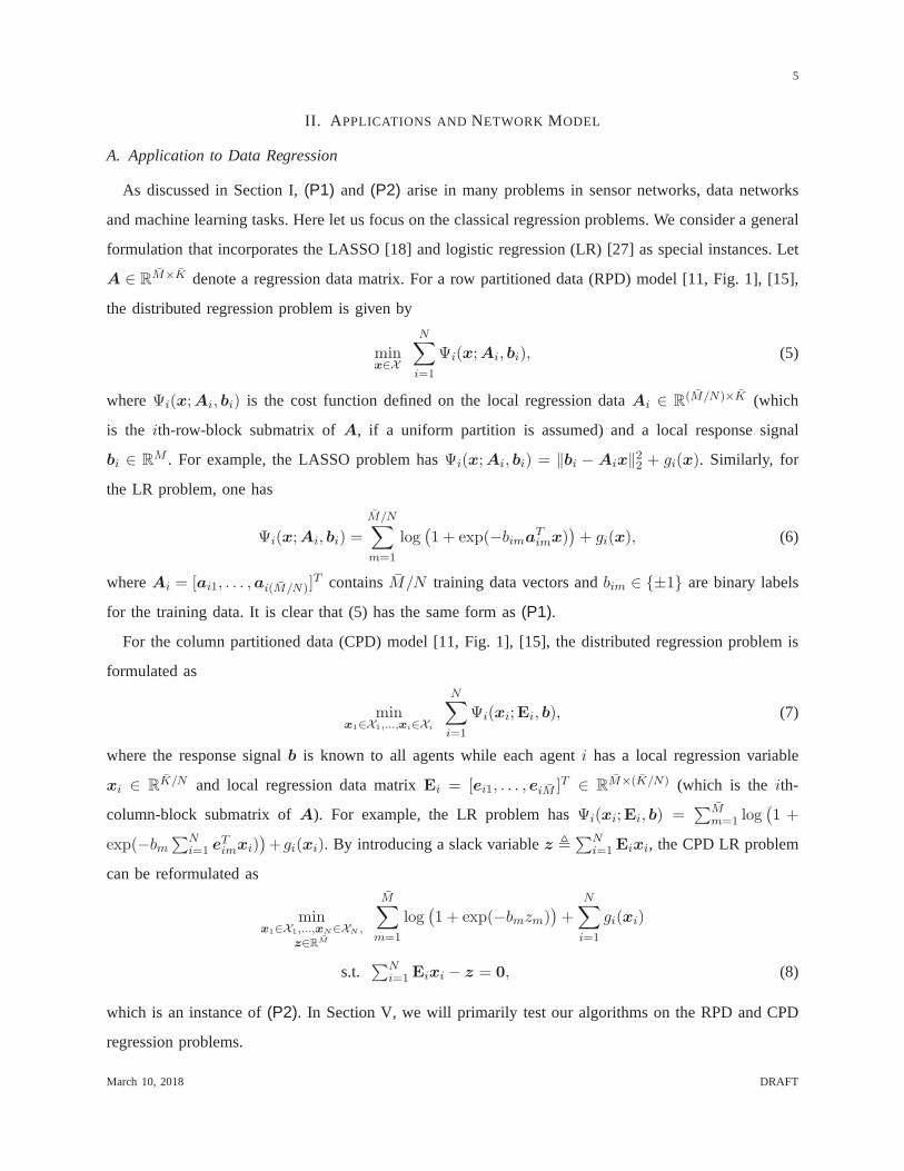
A. Application to Data Regression

As discussed in Section I,(P1) and (P2) arise in many problems in sensor networks, data networks

and machine learning tasks. Here let us focus on the classical regression problems. We consider a general

formulation that incorporates the LASSO [18] and logistic regression (LR) [27] as special instances. Let

A ∈ RM×K denote a regression data matrix. For a row partitioned data (RPD) model [11, Fig. 1], [15],

the distributed regression problem is given by

minx∈X

N∑

i=1

Ψi(x;Ai, bi), (5)

whereΨi(x;Ai, bi) is the cost function defined on the local regression dataAi ∈ R(M/N)×K (which

is the ith-row-block submatrix ofA, if a uniform partition is assumed) and a local response signal

bi ∈ RM . For example, the LASSO problem hasΨi(x;Ai, bi) = ‖bi − Aix‖22 + gi(x). Similarly, for

the LR problem, one has

Ψi(x;Ai, bi) =

M/N∑

m=1

log(

1 + exp(−bimaTimx)

)

+ gi(x), (6)

whereAi = [ai1, . . . ,ai(M/N)]T containsM/N training data vectors andbim ∈ {±1} are binary labels

for the training data. It is clear that (5) has the same form as(P1).

For the column partitioned data (CPD) model [11, Fig. 1], [15], the distributed regression problem is

formulated as

minx1∈X1,...,xi∈Xi

N∑

i=1

Ψi(xi;Ei, b), (7)

where the response signalb is known to all agents while each agenti has a local regression variable

xi ∈ RK/N and local regression data matrixEi = [ei1, . . . ,eiM ]T ∈ R

M×(K/N) (which is the ith-

column-block submatrix ofA). For example, the LR problem hasΨi(xi;Ei, b) =∑M

m=1 log(

1 +

exp(−bm∑N

i=1 eTimxi)

)

+gi(xi). By introducing a slack variablez ,∑N

i=1 Eixi, the CPD LR problem

can be reformulated as

minx1∈X1,...,xN∈XN ,

z∈RM

M∑

m=1

log(

1 + exp(−bmzm))

+

N∑

i=1

gi(xi)

s.t.∑N

i=1Eixi − z = 0, (8)

which is an instance of(P2). In Section V, we will primarily test our algorithms on the RPD and CPD

regression problems.


6

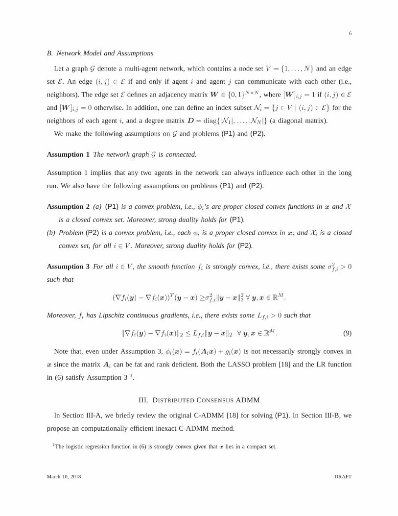
B. Network Model and Assumptions

Let a graphG denote a multi-agent network, which contains a node setV = {1, . . . , N} and an edge

set E . An edge(i, j) ∈ E if and only if agenti and agentj can communicate with each other (i.e.,

neighbors). The edge setE defines an adjacency matrixW ∈ {0, 1}N×N , where[W ]i,j = 1 if (i, j) ∈ Eand [W ]i,j = 0 otherwise. In addition, one can define an index subsetNi = {j ∈ V | (i, j) ∈ E} for the

neighbors of each agenti, and a degree matrixD = diag{|N1|, . . . , |NN |} (a diagonal matrix).

We make the following assumptions onG and problems(P1) and (P2).

Assumption 1 The network graphG is connected.

Assumption 1 implies that any two agents in the network can always influence each other in the long

run. We also have the following assumptions on problems(P1) and (P2).

Assumption 2 (a) (P1) is a convex problem, i.e.,φi’s are proper closed convex functions inx and Xis a closed convex set. Moreover, strong duality holds for(P1).

(b) Problem(P2) is a convex problem, i.e., eachφi is a proper closed convex inxi andXi is a closed

convex set, for alli ∈ V . Moreover, strong duality holds for(P2).

Assumption 3 For all i ∈ V , the smooth functionfi is strongly convex, i.e., there exists someσ2f,i > 0

such that

(∇fi(y)−∇fi(x))T (y − x) ≥σ2

f,i‖y − x‖22 ∀ y,x ∈ RM .

Moreover,fi has Lipschitz continuous gradients, i.e., there exists some Lf,i > 0 such that

‖∇fi(y)−∇fi(x)‖2 ≤ Lf,i‖y − x‖2 ∀ y,x ∈ RM . (9)

Note that, even under Assumption 3,φi(x) = fi(Aix) + gi(x) is not necessarily strongly convex in

x since the matrixAi can be fat and rank deficient. Both the LASSO problem [18] and the LR function

in (6) satisfy Assumption 31.

III. D ISTRIBUTED CONSENSUSADMM

In Section III-A, we briefly review the original C-ADMM [18] for solving(P1). In Section III-B, we

propose an computationally efficient inexact C-ADMM method.

1The logistic regression function in (6) is strongly convex given thatx lies in a compact set.


7

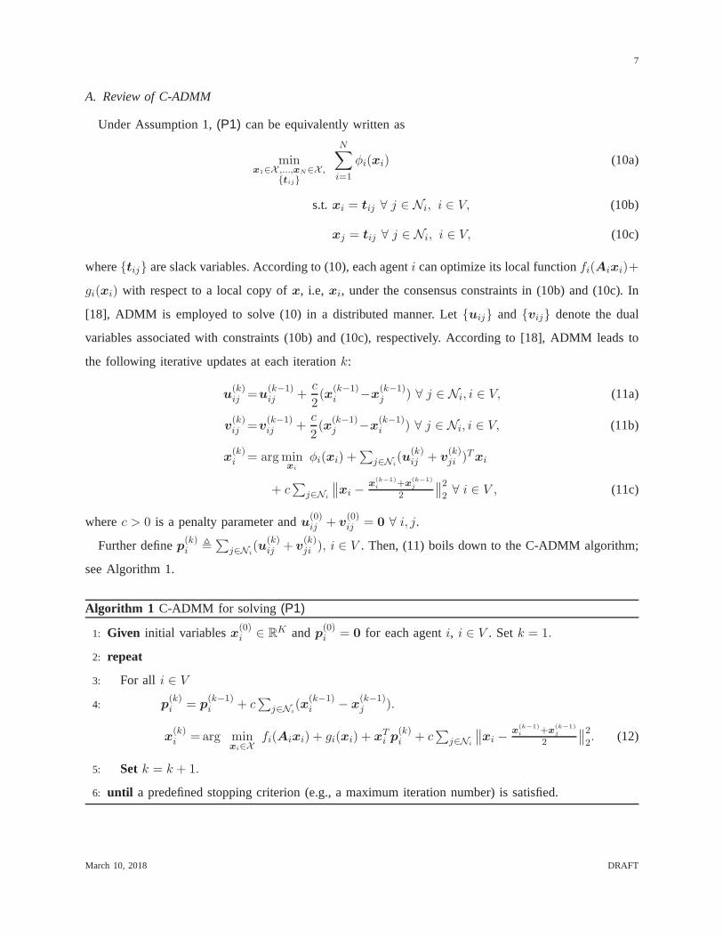
A. Review of C-ADMM

Under Assumption 1,(P1) can be equivalently written as

minx1∈X ,...,xN∈X ,

{tij}

N∑

i=1

φi(xi) (10a)

s.t.xi = tij ∀ j ∈ Ni, i ∈ V, (10b)

xj = tij ∀ j ∈ Ni, i ∈ V, (10c)

where{tij} are slack variables. According to (10), each agenti can optimize its local functionfi(Aixi)+

gi(xi) with respect to a local copy ofx, i.e, xi, under the consensus constraints in (10b) and (10c). In

[18], ADMM is employed to solve (10) in a distributed manner.Let {uij} and {vij} denote the dual

variables associated with constraints (10b) and (10c), respectively. According to [18], ADMM leads to

the following iterative updates at each iterationk:

u(k)ij =u

(k−1)ij +

c

2(x

(k−1)i −x

(k−1)j ) ∀ j ∈ Ni, i ∈ V, (11a)

v(k)ij =v

(k−1)ij +

c

2(x

(k−1)j −x

(k−1)i ) ∀ j ∈ Ni, i ∈ V, (11b)

x(k)i = argmin

xi

φi(xi) +∑

j∈Ni(u

(k)ij + v

(k)ji )Txi

+ c∑

j∈Ni

∥

∥xi − x(k−1)i +x

(k−1)j

2

∥

∥

2

2∀ i ∈ V , (11c)

wherec > 0 is a penalty parameter andu(0)ij + v

(0)ij = 0 ∀ i, j.

Further definep(k)i ,

∑

j∈Ni(u

(k)ij + v

(k)ji ), i ∈ V . Then, (11) boils down to the C-ADMM algorithm;

see Algorithm 1.

Algorithm 1 C-ADMM for solving (P1)

1: Given initial variablesx(0)i ∈ R

K andp(0)i = 0 for each agenti, i ∈ V . Setk = 1.

2: repeat

3: For all i ∈ V

4: p(k)i = p

(k−1)i + c

∑

j∈Ni(x

(k−1)i − x

(k−1)j ).

x(k)i =arg min

xi∈Xfi(Aixi) + gi(xi) + xT

i p(k)i + c

∑

j∈Ni

∥

∥xi − x(k−1)i +x

(k−1)j

2

∥

∥

2

2. (12)

5: Set k = k + 1.

6: until a predefined stopping criterion (e.g., a maximum iteration number) is satisfied.


8

It is important to note from Step 4 and Step 5 of Algorithm 1 that each agenti updates the variables

(x(k)i ,p

(k)i ) in a fully parallel manner, by only using the local functionφi and messages{x(k−1)

j }j∈Ni,

which come from its direct neighbors. It has been shown in [18] that, under Assumptions 1 and 2,

C-ADMM is guaranteed to converge:

limk→∞

x(k)i = x⋆, lim

k→∞(u

(k)ij ,v

(k)ij ) = (u⋆

ij ,v⋆ij), ∀j, i, (13)

wherex⋆ and{u⋆ij ,v

⋆ij} denote the optimal primal solution and dual solution to problem (10) (i.e.,(P1)),

respectively. It is also shown that C-ADMM can converge linearly either whenφi’s are smooth, strongly

convex [23] or whenφi’s satisfy certain error bound assumption [22].

One key issue about C-ADMM is that the subproblem in (12) is not always easy to solve. For instance,

for the LR function in (6), the associated subproblem (12) isgiven by

x(k)i =arg min

xi∈X

M/N∑

m=1

log(

1 + exp(−bimaTimxi)

)

+ gi(xi)

+ xTi p

(k)i + c

∑

j∈Ni

∥

∥xi − x(k−1)i +x

(k−1)j

2

∥

∥

2

2. (14)

As seen, due to the complicated LR cost, problem (14) cannot yield simple solutions, and a numerical

solver has to be employed. Clearly, obtaining a high-accuracy solution of (14) can be computationally

expensive, especially when the problem dimension or the number of training data is large. While a

low-accuracy solution to (14) can be adopted for complexityreduction, it may destroy the convergence

behavior of C-ADMM, as will be shown in Section V.

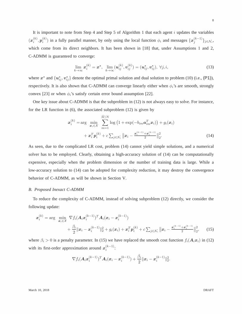
B. Proposed Inexact C-ADMM

To reduce the complexity of C-ADMM, instead of solving subproblem (12) directly, we consider the

following update:

x(k)i = arg min

xi∈X∇fi(Aix

(k−1)i )TAi(xi − x

(k−1)i )

+βi2‖xi − x

(k−1)i ‖22 + gi(xi) + xT

i p(k)i + c

∑

j∈Ni

∥

∥xi − x(k−1)i +x

(k−1)j

2

∥

∥

2

2, (15)

whereβi > 0 is a penalty parameter. In (15) we have replaced the smooth cost functionfi(Aixi) in (12)

with its first-order approximation aroundx(k−1)i :

∇fi(Aix(k−1)i )TAi(xi − x

(k−1)i ) +

βi2‖xi − x

(k−1)i ‖22.


9

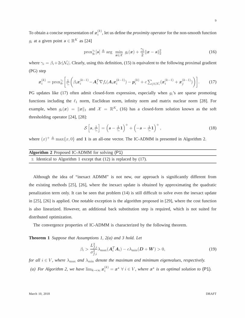
To obtain a concise representation ofx(k)i , let us define theproximity operatorfor the non-smooth function

gi at a given points ∈ RK as [24]

proxγi

gi [s] , arg minx∈X

gi(x) +γi2‖x− s‖22 (16)

whereγi = βi+2c|Ni|. Clearly, using this definition, (15) is equivalent to the following proximal gradient

(PG) step

x(k)i = proxγi

gi

[

1γi

(

βix(k−1)i −AT

i ∇fi(Aix(k−1)i )− p

(k)i + c

∑

j∈Ni(x

(k−1)i + x

(k−1)j )

)]

. (17)

PG updates like (17) often admit closed-form expression, especially whengi’s are sparse promoting

functions including theℓ1 norm, Euclidean norm, infinity norm and matrix nuclear norm [28]. For

example, whengi(x) = ‖x‖1 and X = RK , (16) has a closed-form solution known as the soft

thresholding operator [24], [28]:

S[

s, 1γi

]

=(

s− 1γi1

)++(

−s− 1γi1

)+, (18)

where(x)+ , max{x, 0} and1 is an all-one vector. The IC-ADMM is presented in Algorithm 2.

Algorithm 2 Proposed IC-ADMM for solving(P1)

1: Identical to Algorithm 1 except that (12) is replaced by (17).

Although the idea of “inexact ADMM” is not new, our approach is significantly different from

the existing methods [25], [26], where the inexact update isobtained by approximating the quadratic

penalization term only. It can be seen that problem (14) is still difficult to solve even the inexact update

in [25], [26] is applied. One notable exception is the algorithm proposed in [29], where the cost function

is also linearized. However, an additional back substitution step is required, which is not suited for

distributed optimization.

The convergence properties of IC-ADMM is characterized by the following theorem.

Theorem 1 Suppose that Assumptions 1, 2(a) and 3 hold. Let

βi >L2f,i

σ2f,i

λmax(ATi Ai)− cλmin(D +W ) > 0, (19)

for all i ∈ V , whereλmax and λmin denote the maximum and minimum eigenvalues, respectively.

(a) For Algorithm 2, we havelimk→∞ x(k)i = x⋆ ∀ i ∈ V , wherex⋆ is an optimal solution to(P1).


10

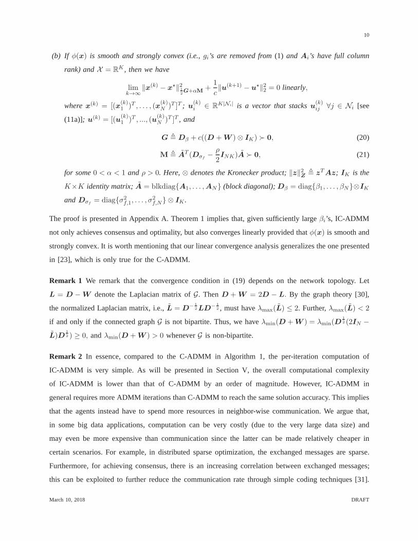
(b) If φ(x) is smooth and strongly convex (i.e.,gi’s are removed from(1) and Ai’s have full column

rank) andX = RK , then we have

limk→∞

‖x(k) − x⋆‖212G+αM +

1

c‖u(k+1) − u⋆‖22 = 0 linearly,

wherex(k) = [(x(k)1 )T , . . . , (x

(k)N )T ]T ; u

(k)i ∈ R

K|Ni| is a vector that stacksu(k)ij ∀j ∈ Ni [see

(11a)]; u(k) = [(u(k)1 )T , ..., (u

(k)N )T ]T , and

G , Dβ + c((D +W )⊗ IK) ≻ 0, (20)

M , AT (Dσf− ρ

2INK)A ≻ 0, (21)

for some0 < α < 1 andρ > 0. Here,⊗ denotes the Kronecker product;‖z‖2Z , zTAz; IK is the

K×K identity matrix;A = blkdiag{A1, . . . ,AN} (block diagonal);Dβ = diag{β1, . . . , βN}⊗IK

andDσf= diag{σ2

f,1, . . . , σ2f,N} ⊗ IK .

The proof is presented in Appendix A. Theorem 1 implies that,given sufficiently largeβi’s, IC-ADMM

not only achieves consensus and optimality, but also converges linearly provided thatφ(x) is smooth and

strongly convex. It is worth mentioning that our linear convergence analysis generalizes the one presented

in [23], which is only true for the C-ADMM.

Remark 1 We remark that the convergence condition in (19) depends on the network topology. Let

L = D −W denote the Laplacian matrix ofG. ThenD + W = 2D − L. By the graph theory [30],

the normalized Laplacian matrix, i.e.,L = D− 1

2LD− 1

2 , must haveλmax(L) ≤ 2. Further,λmax(L) < 2

if and only if the connected graphG is not bipartite. Thus, we haveλmin(D +W ) = λmin(D1

2 (2IN −L)D

1

2 ) ≥ 0, andλmin(D +W ) > 0 wheneverG is non-bipartite.

Remark 2 In essence, compared to the C-ADMM in Algorithm 1, the per-iteration computation of

IC-ADMM is very simple. As will be presented in Section V, theoverall computational complexity

of IC-ADMM is lower than that of C-ADMM by an order of magnitude. However, IC-ADMM in

general requires more ADMM iterations than C-ADMM to reach the same solution accuracy. This implies

that the agents instead have to spend more resources in neighbor-wise communication. We argue that,

in some big data applications, computation can be very costly (due to the very large data size) and

may even be more expensive than communication since the latter can be made relatively cheaper in

certain scenarios. For example, in distributed sparse optimization, the exchanged messages are sparse.

Furthermore, for achieving consensus, there is an increasing correlation between exchanged messages;

this can be exploited to further reduce the communication rate through simple coding techniques [31].


11

Besides, communication via wired links (e.g., database servers connected via dedicated fiber links or

distributed microprocessors connected by data buses) are much more power/time efficient than wireless

links [32]. Therefore, communication are arguably cheaperin these scenarios, and it may be worthy to

trade for complexity reduction.

IV. D ISTRIBUTED DUAL CONSENSUSADMM

In this section, we turn the focus to(P2). In Section IV-A, we present a DC-ADMM method for

solving (P2). In Section IV-B, an inexact DC-ADMM method is proposed.

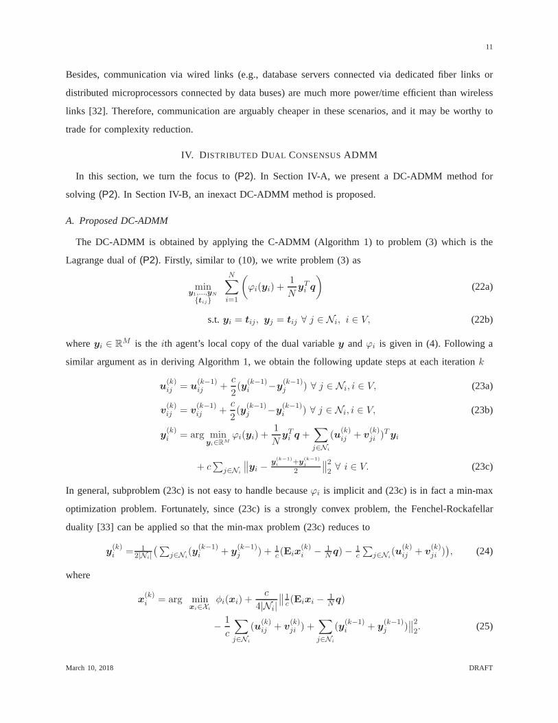
A. Proposed DC-ADMM

The DC-ADMM is obtained by applying the C-ADMM (Algorithm 1)to problem (3) which is the

Lagrange dual of(P2). Firstly, similar to (10), we write problem (3) as

miny1,...,yN

{tij}

N∑

i=1

(

ϕi(yi) +1

NyTi q

)

(22a)

s.t.yi = tij, yj = tij ∀ j ∈ Ni, i ∈ V, (22b)

whereyi ∈ RM is the ith agent’s local copy of the dual variabley andϕi is given in (4). Following a

similar argument as in deriving Algorithm 1, we obtain the following update steps at each iterationk

u(k)ij = u

(k−1)ij +

c

2(y

(k−1)i −y

(k−1)j ) ∀ j ∈ Ni, i ∈ V, (23a)

v(k)ij = v

(k−1)ij +

c

2(y

(k−1)j −y

(k−1)i ) ∀ j ∈ Ni, i ∈ V, (23b)

y(k)i = arg min

yi∈RMϕi(yi) +

1

NyTi q +

∑

j∈Ni

(u(k)ij + v

(k)ji )Tyi

+ c∑

j∈Ni

∥

∥yi − y(k−1)i +y

(k−1)j

2

∥

∥

2

2∀ i ∈ V. (23c)

In general, subproblem (23c) is not easy to handle becauseϕi is implicit and (23c) is in fact a min-max

optimization problem. Fortunately, since (23c) is a strongly convex problem, the Fenchel-Rockafellar

duality [33] can be applied so that the min-max problem (23c)reduces to

y(k)i = 1

2|Ni|

(∑

j∈Ni(y

(k−1)i + y

(k−1)j ) + 1

c (Eix(k)i − 1

N q)− 1c

∑

j∈Ni(u

(k)ij + v

(k)ji )

)

, (24)

where

x(k)i = arg min

xi∈Xi

φi(xi) +c

4|Ni|∥

∥

1c (Eixi − 1

N q)

− 1

c

∑

j∈Ni

(u(k)ij + v

(k)ji ) +

∑

j∈Ni

(y(k−1)i + y

(k−1)j )

∥

∥

2

2. (25)


12

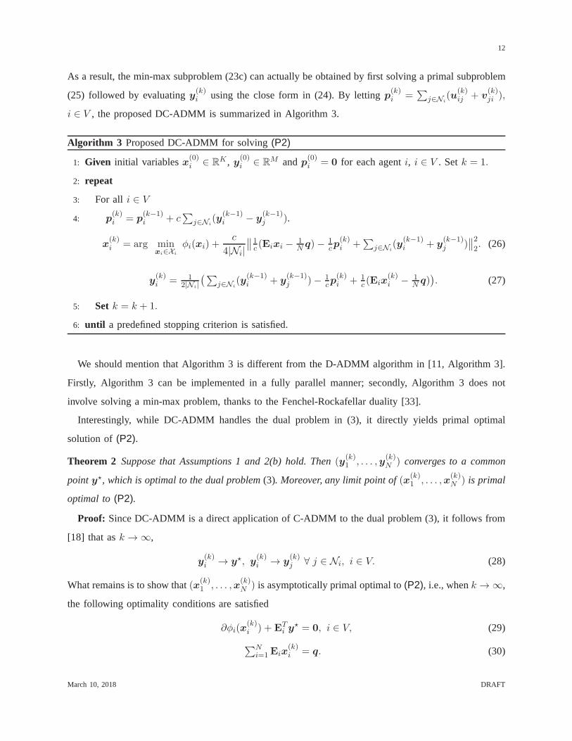
As a result, the min-max subproblem (23c) can actually be obtained by first solving a primal subproblem

(25) followed by evaluatingy(k)i using the close form in (24). By lettingp(k)

i =∑

j∈Ni(u

(k)ij + v

(k)ji ),

i ∈ V , the proposed DC-ADMM is summarized in Algorithm 3.

Algorithm 3 Proposed DC-ADMM for solving(P2)

1: Given initial variablesx(0)i ∈ R

K , y(0)i ∈ R

M andp(0)i = 0 for each agenti, i ∈ V . Setk = 1.

2: repeat

3: For all i ∈ V

4: p(k)i = p

(k−1)i + c

∑

j∈Ni(y

(k−1)i − y

(k−1)j ).

x(k)i = arg min

xi∈Xi

φi(xi) +c

4|Ni|∥

∥

1c (Eixi − 1

N q)− 1cp

(k)i +

∑

j∈Ni(y

(k−1)i + y

(k−1)j )

∥

∥

2

2. (26)

y(k)i = 1

2|Ni|

(∑

j∈Ni(y

(k−1)i + y

(k−1)j )− 1

cp(k)i + 1

c (Eix(k)i − 1

N q))

. (27)

5: Set k = k + 1.

6: until a predefined stopping criterion is satisfied.

We should mention that Algorithm 3 is different from the D-ADMM algorithm in [11, Algorithm 3].

Firstly, Algorithm 3 can be implemented in a fully parallel manner; secondly, Algorithm 3 does not

involve solving a min-max problem, thanks to the Fenchel-Rockafellar duality [33].

Interestingly, while DC-ADMM handles the dual problem in (3), it directly yields primal optimal

solution of (P2).

Theorem 2 Suppose that Assumptions 1 and 2(b) hold. Then(y(k)1 , . . . ,y

(k)N ) converges to a common

pointy⋆, which is optimal to the dual problem(3). Moreover, any limit point of(x(k)1 , . . . ,x

(k)N ) is primal

optimal to (P2).

Proof: Since DC-ADMM is a direct application of C-ADMM to the dual problem (3), it follows from

[18] that ask → ∞,

y(k)i → y⋆, y

(k)i → y

(k)j ∀ j ∈ Ni, i ∈ V. (28)

What remains is to show that(x(k)1 , . . . ,x

(k)N ) is asymptotically primal optimal to(P2), i.e., whenk → ∞,

the following optimality conditions are satisfied

∂φi(x(k)i ) +E

Ti y

⋆ = 0, i ∈ V, (29)

∑Ni=1Eix

(k)i = q. (30)


13

To show (29), consider the optimality condition of (25), i.e.,

0 = ∂φi(x(k)i ) +

1

2|Ni|E

Ti

(

1

c(Eix

(k)i − 1

Nq)

− 1c

∑

j∈Ni(u

(k)ij + v

(k)ji ) +

∑

j∈Ni(y

(k−1)i + y

(k−1)j )

)

= ∂φi(x(k)i ) +E

Ti y

(k)i , (31)

where the second equality is obtained by (24). Equation (31)infers (29) sincey(k)i → y⋆ by (28).

To show (30), rewrite (24) as follows

0 = −(Eix(k)i − 1

Nq) + 2c

∑

j∈Ni

(

y(k)i − y

(k)i +y

(k)j

2

)

+∑

j∈Ni

(u(k)ij + v

(k)ji )+c

∑

j∈Ni

(y(k)i + y

(k)j − y

(k−1)i − y

(k−1)j )

= −(Eix(k)i − 1

Nq) +

∑

j∈Ni

(u(k+1)ij + v

(k+1)ji ) + c

∑

j∈Ni

(y(k)i + y

(k)j − y

(k−1)i − y

(k−1)j ), (32)

where the last equality is obtained by (23a) and (23b). Upon summing (32) overi = 1, . . . , N , and by

applying (A.11) and (A.12), we can obtain

N∑

i=1

Eix(k)i − q = c

N∑

i=1

∑

j∈Ni

(y(k)i + y

(k)j − y

(k−1)i − y

(k−1)j ). (33)

Finally, by applying (28) to (33), one obtains (30). �

Interestingly, from (33), one observes that the primal feasibility of (x(k)1 , . . . ,x

(k)N ) to (P2) depends

on the agents’ consensus on the dual variabley.

B. Proposed Inexact DC-ADMM

In this subsection, we propose an inexact version of DC-ADMM, referred to as the IDC-ADMM. In

view of the fact that solving the subproblem in (25) can be expensive, we consider an inexact update of

x(k)i . Specifically, since a non-trivialEi can also complicate the solution, we propose to approximateboth

fi(Aixi) and the quadratic term c4|Ni|

‖1c (Eixi− 1

N q)− 1c

∑

j∈Ni(u

(k)ij +v

(k)ji )+

∑

j∈Ni(y

(k−1)i +y

(k−1)j )‖22

in (25) by their first-order approximations aroundx(k−1)i . One can show that this is equivalent to the

following update

x(k)i = arg min

xi∈Xi

(∇fi(Aix(k−1)i ))TAi(xi − x

(k−1)i ) + gi(xi)

+ 12(xi − x

(k−1)i )TPi(xi − x

(k−1)i ) + c

4|Ni|

∥

∥

1c (Eixi − 1

N q)

− 1cp

(k)i +

∑

j∈Ni(y

(k−1)i + y

(k−1)j )

∥

∥

2

2, (34)


14

where2

Pi = βiIK − 12c|Ni|

ETi Ei.

By (16), (34) is equivalent to the following PG update

x(k)i = proxβi

gi

[

x(k−1)i − 1

βiAT

i ∇fi(Aix(k−1)i )(Eix

(k−1)i − 1

N q)

− 12βi|Ni|

ETi

(

− p(k)i + c

∑

j∈Ni(y

(k−1)i + y

(k−1)j )

)

]

. (35)

We summarize the proposed IDC-ADMM in Algorithm 4.

Algorithm 4 Proposed IDC-ADMM for solving(P2)

1: Identical to Algorithm 3 except that (26) is replaced by (35).

The convergence property of IDC-ADMM is stated below.

Theorem 3 Suppose that Assumptions 1, 2(b) and 3 hold. Let

Pi −L2f,i

σ2f,i

ATi Ai ≻ 0 ∀ i ∈ V. (36)

(a) The sequence(x(k)1 , . . . ,x

(k)N ) generated from Algorithm 4 converges to an optimal solutionx⋆ =

[(x(k)1 )T , . . . , (x

(k)N )T ]T to (P2) while (y

(k)1 , . . . ,y

(k)N ) converges to a common pointy⋆ which is

optimal to problem(3).

(b) Suppose that eachφi(xi) is smooth and strongly convex inxi, Ei’s have full row rank andXi = RK

for all i ∈ V . Then, for some0 < α < 1 and ρ > 0, we have

‖x(k) − x⋆‖2αM+ 1

2P+

1

c‖u(k+1) − u⋆‖22

+c

2‖y(k) − y⋆‖2(D+W )⊗IM

→ 0 linearly, (37)

whereM is defined in(21), y⋆ , 1N ⊗ y⋆ andP , blkdiag{P1, . . . ,PN} ≻ 0.

The proof is presented in Appendix B. Note that, in addition to the smooth and strongly convex objective

function, IDC-ADMM also requires matricesEi’s to have full row rank in order to have a linear

convergence rate.

2WhenEi has orthogonal columns (e.g.,ET

i Ei = αI for someα ∈ R), then it may not be necessary to approximate the

quadratic term. In that case, one instead setsPi = βiIK .


15

V. NUMERICAL RESULTS

In this section, we examine the numerical performance of Algorithm 1 to 4 presented so far.

A. Performance of C-ADMM and IC-ADMM

To test C-ADMM (Algorithm 1) and IC-ADMM (Algorithm 2), we considered the distributed RPD

LR problem in (5) and (6), withgi(x) = λN ‖x‖1 serving as a sparsity promoting function, where

λ > 0 is a penalty parameter. We considered a simple two image classification task. Specifically, we

used the images D24 and D68 from the Brodatz data set (http://www.ux.uis.no/∼tranden/brodatz.html) to

generate the regression data matrixA. We randomly extractedM/2 overlapping patches with dimension√K ×

√K from the two images, respectively, followed by vectorizingthe M patches into vectors and

stacking all of them into anM × K matrix. The rows of the matrix were randomly shuffled and the

resultant matrix was used as the data matrixA. For the RPD LR problem (5), we horizontally partitioned

the matrixA into N submatricesA1, . . . ,AN , each with dimension(M/N)× K. These matrices were

used as the training data. Note that eachAi contains patches from both images. The binary labelsbi’s

then were generated accordingly with1 for one image and−1 for the other. The feasible set was set to

X = {x ∈ RK | |xi| ≤ a ∀ i} for somea > 0. The graphG was randomly generated.

To implement Algorithm 1, we employed the fast iterative shrinkage thresholding algorithm (FISTA)

[34], [35] to solve subproblem (12) for each agenti. For (12), the associated FISTA steps can be shown

as

x(ℓ)i = max

{

−a,min

{

a,S[

z(ℓ−1)i − ρ

(ℓ)i

[

ATi ∇fi(Aiz

(ℓ−1)i )

+p(k)i +2c

∑

j∈Ni

(z(ℓ−1)i −

x(k−1)i + x

(k−1)j

2)

]

,λρ

(ℓ)i

N

]}}

, (38a)

z(ℓ)i = x

(ℓ)i +

ℓ− 1

ℓ+ 2(x

(ℓ)i − x

(ℓ−1)i ), (38b)

where ℓ denotes the inner iteration index of FISTA,ρ(ℓ)i > 0 is a step size andS is defined in (18).

Suppose that FISTA stops at iterationℓi(k). We then setx(k)i = x

(ℓi(k))i as a solution to subproblem

(12). The stopping criterion of (38) was based on the PG residue (pgr) pgr = ‖z(ℓ−1)i − x

(ℓ)i ‖/(ρ(ℓ)i

√K)

[34], [35]. For obtaining a high-accuracy solution of (12),one may set the stopping criterion as, e.g.,

pgr < 10−5.


16

For IC-ADMM, the corresponding step in (17) is given by

x(k)i =max

{

− a,min

{

a,1

γiS[

βx(k−1)i −AT

i ∇fi(Aix(k−1)i )

− p(k)i + c

∑

j∈Ni

(x(k−1)i + x

(k−1)j ),

λ

N

]}}

. (39)

By comparing (39) with (38a), one can see that, for each agenti, the computational complexity of

Algorithm 1 per iterationk (we refer this as the “ADMM iteration (ADMM Ite.)”) is roughly ℓi(k)

times that of Algorithm 2. To measure the computational complexity of Algorithm 1, we count the total

average number of FISTA iterations implemented by each agent before Algorithm 1 stops. More precisely,

suppose that the total number of ADMM iterations of Algorithm 1 is Icm. The complexity per agent due

to Algorithm 1 is measured by the computation iteration:

Compt. Ite. = 1N

∑Icmk=1

∑Ni=1 ℓi(k). (40)

By contrast, the complexity per agent due to Algorithm 2 is simply given by Icm if the total number

of ADMM iterations of Algorithm 2 is Icm. The stopping criterion of Algorithms 1 and 2 was based

on measuring the solution accuracyacc = (obj(x(k))− obj⋆)/obj⋆ and variable consensus errorcserr =∑N

i=1 ‖x(k) − x(k)i ‖22/N , where x(k) = (

∑Ni=1 x

(k)i )/N , obj(x(k)) denotes the objective value of (5)

given x = x(k), andobj⋆ is the optimal value of (5) which was obtained by FISTA [34], [35] with a

high solution accuracy ofpgr < 10−6. The two algorithms were set to stop wheneveracc andcserr are

both smaller than preset target values.

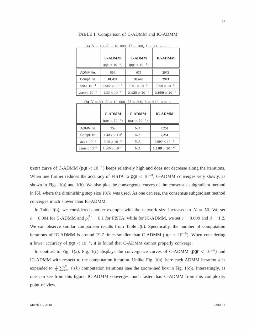
In Table I(a), we considered a simulation example ofN = 10, K = 10, 000, M = 100, λ = 0.1,

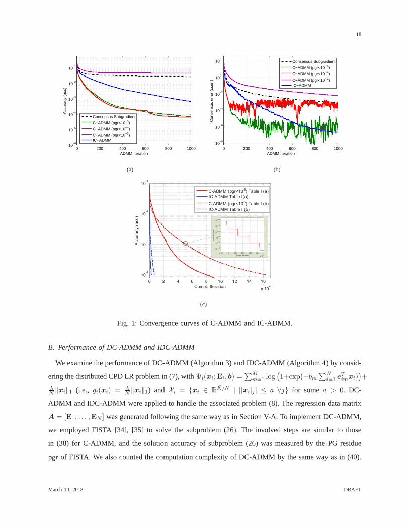
a = 1, and display the comparison results. The convergence curves of C-ADMM and IC-ADMM with

respect to the ADMM iteration are also shown in Figs. 1(a) and1(b). The stopping conditions areacc

< 10−4 and cserr < 10−5. For C-ADMM, we considered two cases, one with the stopping condition

of FISTA for solving subproblem (12) set topgr < 10−5 and the other with that set topgr < 10−4.

The penalty parameterc for C-ADMM was set toc = 0.03 and the step sizeρ(ℓ)i of FISTA (see (38))

was set to a constantρ(ℓ)i = 0.1. The penalty parametersc andβ of IC-ADMM were set toc = 0.01

and β = 1.2. We observe from Table I(a) that IC-ADMM in general requiresmore ADMM iterations

than C-ADMM; however, the required computation complexityis significantly lower. Specifically, the

number of computation iterations of IC-ADMM is around81, 459/2973 ≈ 27.4 times smaller than that of

C-ADMM (pgr < 10−5). We also observe that C-ADMM (pgr < 10−4) consumes a smaller number of

computation iterations for achievingacc < 10−4. However, the associatedcserr = 3.425× 10−4 is quite

large. In fact, C-ADMM (pgr < 10−4) cannot reducecserr properly. As one can see from Fig. 1(b), the


17

TABLE I: Comparison of C-ADMM and IC-ADMM

(a) N = 10, K = 10, 000, M = 100, λ = 0.1, a = 1.

C-ADMM C-ADMM IC-ADMM

(pgr < 10−5) (pgr < 10−4)

ADMM Ite. 810 675 2973

Compt. Ite. 81,459 30,648 2973

acc< 10−4 9.982 × 10−5 9.91 × 10−5 9.99× 10−5

cserr< 10−5 1.53× 10−63.425× 10

−43.859× 10

−9

(b) N = 50, K = 10, 000, M = 500, λ = 0.15, a = 1.

C-ADMM C-ADMM IC-ADMM

(pgr < 10−5) (pgr < 10−4)

ADMM Ite. 952 N/A 7,251

Compt. Ite. 1.432× 105 N/A 7,251

acc< 10−4 9.99× 10−5 N/A 9.999 × 10−5

cserr< 10−5 1.305 × 10−7 N/A 1.169× 10−10

cserr curve of C-ADMM (pgr < 10−4) keeps relatively high and does not decrease along the iterations.

When one further reduces the accuracy of FISTA topgr < 10−3, C-ADMM converges very slowly, as

shown in Figs. 1(a) and 1(b). We also plot the convergence curves of the consensus subgradient method

in [6], where the diminishing step size10/k was used. As one can see, the consensus subgradient method

converges much slower than IC-ADMM.

In Table I(b), we considered another example with the network size increased toN = 50. We set

c = 0.004 for C-ADMM and ρ(ℓ)i = 0.1 for FISTA; while for IC-ADMM, we setc = 0.008 andβ = 1.2.

We can observe similar comparison results from Table I(b). Specifically, the number of computation

iterations of IC-ADMM is around 19.7 times smaller than C-ADMM (pgr < 10−5). When considering

a lower accuracy ofpgr < 10−4, it is found that C-ADMM cannot properly converge.

In contrast to Fig. 1(a), Fig. 1(c) displays the convergencecurves of C-ADMM (pgr < 10−5) and

IC-ADMM with respect to the computation iteration. Unlike Fig. 1(a), here each ADMM iterationk is

expanded to1N

∑Ni=1 ℓi(k) computation iterations (see the zoom-ined box in Fig. 1(c)). Interestingly, as

one can see from this figure, IC-ADMM converges much faster than C-ADMM from this complexity

point of view.


18

0 200 400 600 800 100010

−6

10−5

10−4

10−3

10−2

10−1

ADMM Iteration

Acc

urac

y (a

cc)

Consensus Subgradient

C−ADMM (pgr<10−5)


C−ADMM (pgr<10−3)IC−ADMM

(a)

0 200 400 600 800 100010

−8

10−6

10−4

10−2

100

102

ADMM Iteration

Con

sens

us e

rror

(cs

err)

Consensus Subgradient



C−ADMM (pgr<10−3)IC−ADMM

(b)

0 2 4 6 8 10 12 14 16

x 104

10-4

10-3

10-2

10-1

Compt. Iteration

Accu

racy (

acc)

C-ADMM (pgr<10-5) Table I (a)

IC-ADMM Table I(a)

C-ADMM (pgr<10-5) Table I (b)

IC-ADMM Table I (b)

4.99 5 5.01 5.02 5.03 5.04

x 104

10-3.074

10-3.072

10-3.07

10-3.068

10-3.066

10-3.064

Compt. Iteration

Acc

ura

cy (

acc)

(c)

Fig. 1: Convergence curves of C-ADMM and IC-ADMM.

B. Performance of DC-ADMM and IDC-ADMM

We examine the performance of DC-ADMM (Algorithm 3) and IDC-ADMM (Algorithm 4) by consid-

ering the distributed CPD LR problem in (7), withΨi(xi;Ei, b) =∑M

m=1 log(

1+exp(−bm∑N

i=1 eTimxi)

)

+

λN ‖xi‖1 (i.e., gi(xi) = λ

N ‖xi‖1) and Xi = {xi ∈ RK/N | |[xi]j | ≤ a ∀j} for somea > 0. DC-

ADMM and IDC-ADMM were applied to handle the associated problem (8). The regression data matrix

A = [E1, . . . ,EN ] was generated following the same way as in Section V-A. To implement DC-ADMM,

we employed FISTA [34], [35] to solve the subproblem (26). The involved steps are similar to those

in (38) for C-ADMM, and the solution accuracy of subproblem (26) was measured by the PG residue

pgr of FISTA. We also counted the computation complexity of DC-ADMM by the same way as in (40).


19

Similarly, the stopping criterion of Algorithms 3 and 4 was based on measuring the solution accuracy

acc = (obj(x(k))− obj⋆)/obj⋆, wherex(k) = [(x(k)1 )T , . . . , (x

(k)N )T ]T , obj(x(k)) denotes the objective

value of (7) andobj⋆ is the optimal value of (7) obtained by using FISTA with a highaccuracy of

pgr < 1e−6. Unlike Section V-A, here for problem (7) we did not care the consensus of{y(k)i } or the

satisfaction of constraint∑N

i=1 Eix(k)i = z(k) sincex(k) is always feasible and is an approximate solution

to the original problem (7).

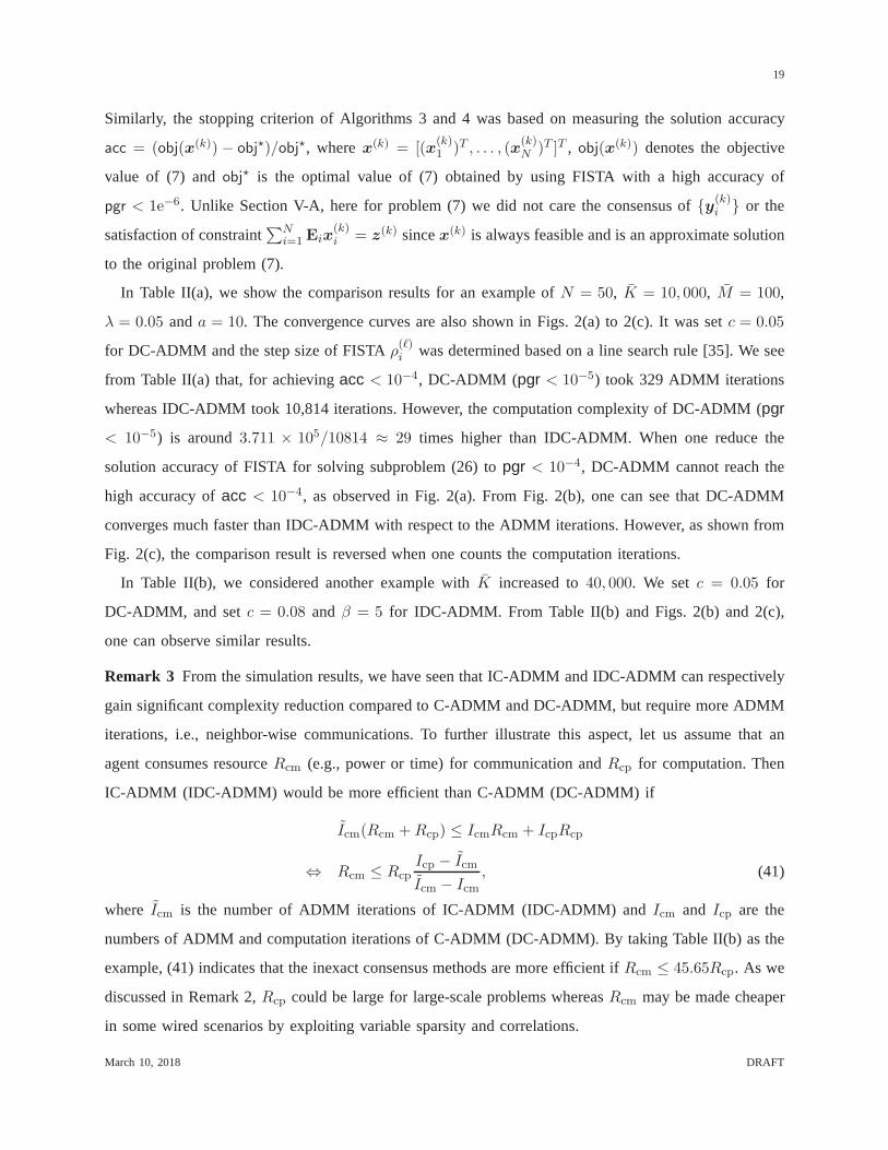
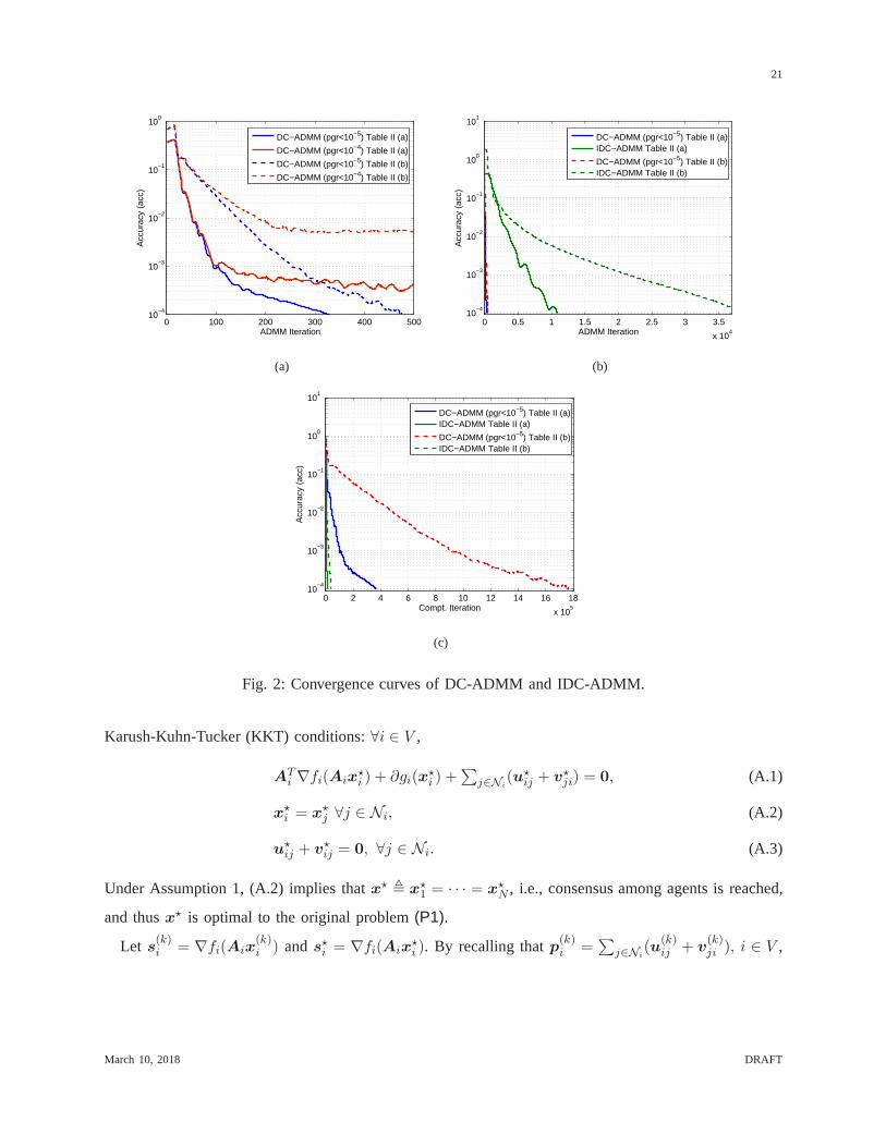
In Table II(a), we show the comparison results for an exampleof N = 50, K = 10, 000, M = 100,

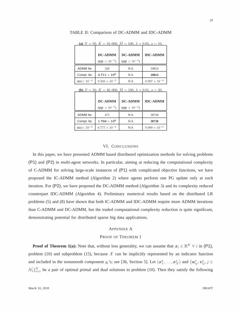
λ = 0.05 anda = 10. The convergence curves are also shown in Figs. 2(a) to 2(c).It was setc = 0.05

for DC-ADMM and the step size of FISTAρ(ℓ)i was determined based on a line search rule [35]. We see

from Table II(a) that, for achievingacc < 10−4, DC-ADMM (pgr < 10−5) took 329 ADMM iterations

whereas IDC-ADMM took 10,814 iterations. However, the computation complexity of DC-ADMM (pgr

< 10−5) is around3.711 × 105/10814 ≈ 29 times higher than IDC-ADMM. When one reduce the

solution accuracy of FISTA for solving subproblem (26) topgr < 10−4, DC-ADMM cannot reach the

high accuracy ofacc < 10−4, as observed in Fig. 2(a). From Fig. 2(b), one can see that DC-ADMM

converges much faster than IDC-ADMM with respect to the ADMMiterations. However, as shown from

Fig. 2(c), the comparison result is reversed when one countsthe computation iterations.

In Table II(b), we considered another example withK increased to40, 000. We setc = 0.05 for

DC-ADMM, and setc = 0.08 andβ = 5 for IDC-ADMM. From Table II(b) and Figs. 2(b) and 2(c),

one can observe similar results.

Remark 3 From the simulation results, we have seen that IC-ADMM and IDC-ADMM can respectively

gain significant complexity reduction compared to C-ADMM and DC-ADMM, but require more ADMM

iterations, i.e., neighbor-wise communications. To further illustrate this aspect, let us assume that an

agent consumes resourceRcm (e.g., power or time) for communication andRcp for computation. Then

IC-ADMM (IDC-ADMM) would be more efficient than C-ADMM (DC-ADMM) if

Icm(Rcm +Rcp) ≤ IcmRcm + IcpRcp

⇔ Rcm ≤ RcpIcp − Icm

Icm − Icm, (41)

where Icm is the number of ADMM iterations of IC-ADMM (IDC-ADMM) andIcm and Icp are the

numbers of ADMM and computation iterations of C-ADMM (DC-ADMM). By taking Table II(b) as the

example, (41) indicates that the inexact consensus methodsare more efficient ifRcm ≤ 45.65Rcp. As we

discussed in Remark 2,Rcp could be large for large-scale problems whereasRcm may be made cheaper

in some wired scenarios by exploiting variable sparsity andcorrelations.


20

TABLE II: Comparison of DC-ADMM and IDC-ADMM

(a) N = 50, K = 10, 000, M = 100, λ = 0.05, a = 10.

DC-ADMM DC-ADMM IDC-ADMM

(pgr < 10−5) (pgr < 10−4)

ADMM Ite. 329 N/A 10814

Compt. Ite. 3.711× 105 N/A 10814

acc< 10−4 9.928 × 10−5 N/A 9.997 × 10−4

(b) N = 50, K = 40, 000, M = 100, λ = 0.01, a = 20.

DC-ADMM DC-ADMM IDC-ADMM

(pgr < 10−5) (pgr < 10−4)

ADMM Ite. 475 N/A 38728

Compt. Ite. 1.768× 106 N/A 38728

acc< 10−4 9.777 × 10−4 N/A 9.999 × 10−5

VI. CONCLUSIONS

In this paper, we have presented ADMM based distributed optimization methods for solving problems

(P1) and (P2) in multi-agent networks. In particular, aiming at reducingthe computational complexity

of C-ADMM for solving large-scale instances of(P1) with complicated objective functions, we have

proposed the IC-ADMM method (Algorithm 2) where agents perform one PG update only at each

iteration. For(P2), we have proposed the DC-ADMM method (Algorithm 3) and its complexity reduced

counterpart IDC-ADMM (Algorithm 4). Preliminary numerical results based on the distributed LR

problems (5) and (8) have shown that both IC-ADMM and IDC-ADMM require more ADMM iterations

than C-ADMM and DC-ADMM, but the traded computational complexity reduction is quite significant,

demonstrating potential for distributed sparse big data applications.

APPENDIX A

PROOF OFTHEOREM 1

Proof of Theorem 1(a): Note that, without loss generality, we can assume thatxi ∈ RK ∀ i in (P1),

problem (10) and subproblem (15), becauseX can be implicitly represented by an indicator function

and included in the nonsmooth componentgi’s; see [36, Section 5]. Let(x⋆1, . . . ,x

⋆N ) and{u⋆

ij ,v⋆ij, j ∈

Ni}Ni=1 be a pair of optimal primal and dual solutions to problem (10). Then they satisfy the following


21

0 100 200 300 400 50010

−4

10−3

10−2

10−1

100

ADMM Iteration

Acc

urac

y (a

cc)

DC−ADMM (pgr<10−5) Table II (a)

DC−ADMM (pgr<10−4) Table II (a)

DC−ADMM (pgr<10−5) Table II (b)

DC−ADMM (pgr<10−4) Table II (b)

(a)

0 0.5 1 1.5 2 2.5 3 3.5

x 104

10−4

10−3

10−2

10−1

100

101

ADMM Iteration

Acc

urac

y (a

cc)

DC−ADMM (pgr<10−5) Table II (a)IDC−ADMM Table II (a)

DC−ADMM (pgr<10−5) Table II (b)IDC−ADMM Table II (b)

(b)

0 2 4 6 8 10 12 14 16 18

x 105

10−4

10−3

10−2

10−1

100

101

Compt. Iteration

Acc

urac

y (a

cc)

DC−ADMM (pgr<10−5) Table II (a)IDC−ADMM Table II (a)

DC−ADMM (pgr<10−5) Table II (b)IDC−ADMM Table II (b)

(c)

Fig. 2: Convergence curves of DC-ADMM and IDC-ADMM.

Karush-Kuhn-Tucker (KKT) conditions:∀i ∈ V ,

ATi ∇fi(Aix

⋆i ) + ∂gi(x

⋆i ) +

∑

j∈Ni(u⋆

ij + v⋆ji) = 0, (A.1)

x⋆i = x⋆

j ∀j ∈ Ni, (A.2)

u⋆ij + v⋆

ij = 0, ∀j ∈ Ni. (A.3)

Under Assumption 1, (A.2) implies thatx⋆ , x⋆1 = · · · = x⋆

N , i.e., consensus among agents is reached,

and thusx⋆ is optimal to the original problem(P1).

Let s(k)i = ∇fi(Aix(k)i ) ands⋆i = ∇fi(Aix

⋆i ). By recalling thatp(k)

i =∑

j∈Ni(u

(k)ij + v

(k)ji ), i ∈ V ,


22

and by the optimality condition of (15) [14] and (A.1), we have that

ATi s

(k−1)i + βi(x

(k)i − x

(k−1)i ) + ∂gi(x

(k)i )

+∑

j∈Ni(u

(k)ij + v

(k)ji ) + 2c

∑

j∈Ni

(

x(k)i − x

(k−1)i +x

(k−1)j

2

)

= 0 = ATi s

⋆i + ∂gi(x

⋆i ) +

∑

j∈Ni(u⋆

ij + v⋆ji). (A.4)

Adding and subtractingATi s

(k)i in the left hand side (LHS) of (A.4) followed by multiplying(x(k)

i −x⋆)

on both sides yields

(s(k−1)i − s

(k)i )TAi(x

(k)i − x⋆) + βi(x

(k)i − x

(k−1)i )T (x

(k)i − x⋆) + (s

(k)i − s⋆i )

TAi(x(k)i − x⋆)

+ (∂gi(x(k)i )− ∂gi(x

⋆))T (x(k)i − x⋆) +

∑

j∈Ni(u

(k)ij − u⋆

ij + v(k)ji − v⋆

ji)T (x

(k)i − x⋆)

+ 2c∑

j∈Ni

(

x(k)i − x

(k−1)i +x

(k−1)j

2

)T

(x(k)i − x⋆) = 0. (A.5)

Note that the first term on the LHS of (A.5) can be lower boundedas

(s(k−1)i − s

(k)i )TAi(x

(k)i − x⋆)

≥ −1

2ρ‖s(k−1)

i − s(k)i ‖22 −

ρ

2‖x(k)

i − x⋆‖2ATi Ai

≥ −L2f,i

2ρ ‖x(k−1)i − x

(k)i ‖2

ATi Ai

− ρ2‖x

(k)i − x⋆‖2

ATi Ai

(A.6)

for anyρ > 0, where the second inequality is due to (9) in Assumption 3. Bythe strong convexity offi

and convexity ofgi, the third and fourth terms of (A.5) can respectively be lower bounded as

(s(k)i − s⋆i )

TAi(x(k)i − x⋆) ≥ σ2

f,i‖x(k)i − x⋆‖2AT

i Ai, (A.7)

(∂gi(x(k)i )− ∂gi(x

⋆))T (x(k)i − x⋆) ≥ 0. (A.8)

Moreover, it follows from (11a) and (11b) that the fifth term of (A.5) can be expressed as

∑

j∈Ni(u

(k)ij − u⋆

ij + v(k)ji − v⋆

ji) =∑

j∈Ni(u

(k+1)ij − u⋆

ij

+ v(k+1)ji − v⋆

ji)− 2c∑

j∈Ni

(

x(k)i − x

(k)i +x

(k)j

2

)

. (A.9)

By substituting (A.6) to (A.9) into (A.5) and summing overi = 1, . . . , N , we obtain

‖x(k) − x⋆‖2M − 1

2ρ‖x(k−1) − x(k)‖2

ATDLfA+ (x(k) − x(k−1))TDβ(x

(k) − x⋆)

+

N∑

i=1

∑

j∈Ni

(u(k+1)ij − u⋆

ij)T (x

(k)i − x⋆

i ) +

N∑

i=1

∑

j∈Ni

(v(k+1)ji − v⋆

ji)T (x

(k)i − x⋆

i )

+ 2c

N∑

i=1

∑

j∈Ni

(

x(k)i + x

(k)j

2−

x(k−1)i + x

(k−1)j

2

)T

(x(k)i − x⋆

i ) ≤ 0, (A.10)


23

wherex(k) = [(x(k)1 )T , . . . , (x

(k)N )T ]T , A = blkdiag{A1, . . . ,AN}, DLf

= diag{L2f,1, . . . , L

2f,N}⊗ IK ,

Dβ = diag{β1, . . . , βN} ⊗ IK andM is defined in (21).

It can be observed from (11a) and (11b) that

u(k)ij + v

(k)ij = 0 ∀j, i, k, (A.11)

given the initialu(0)ij + v

(0)ij = 0 ∀j, i, k. Besides, due to the symmetric property ofW , for any {αij},

we haveN∑

i=1

∑

j∈Ni

αij =

N∑

i=1

N∑

j=1

[W ]i,jαij

=N∑

i=1

N∑

j=1

[W ]i,jαji =N∑

i=1

∑

j∈Ni

αji. (A.12)

By the above two properties and the fact ofu⋆ij + v⋆

ij = 0 ∀j ∈ Ni [Eqn. (A.3)], the fourth and fifth

terms in the LHS of (A.10) can be written as

∑Ni=1

∑

j∈Ni(u

(k+1)ij − u⋆

ij)T (x

(k)i − x⋆)

+∑N

i=1

∑

j∈Ni(v

(k+1)ji − v⋆

ji)T (x

(k)i − x⋆)

=∑N

i=1

∑

j∈Ni(u

(k+1)ij − u⋆

ij)T (x

(k)i − x

(k)j )

= 2c

∑Ni=1

∑

j∈Ni(u

(k+1)ij − u⋆

ij)T (u

(k+1)ij − u

(k)ij )

,2

c(u(k+1) − u⋆)T (u(k+1) − u(k)), (A.13)

where the second equality is owing to (11a), andu(k) is a vector that stacksu(k)ij for all j ∈ Ni,

i = 1, . . . , N . The sixth term in the LHS of (A.10) can be rearranged as follows

c∑N

i=1

∑

j∈Ni(x

(k)i − x

(k−1)i )T (x

(k)i − x⋆)

+ c∑N

i=1

∑

j∈Ni(x

(k)j − x

(k−1)j )T (x

(k)i − x⋆)

= c∑N

i=1 |Ni|(x(k)i − x

(k−1)i )T (x

(k)i − x⋆)

+ c∑N

i=1

∑Nj=1[W ]i,j(x

(k)j − x

(k−1)j )T (x

(k)i − x⋆)

= c(x(k) − x(k−1))T [(D +W )⊗ IK ](x(k) − x⋆), (A.14)

where x⋆ = 1N ⊗ x⋆. Let L = D − W be the Laplacian matrix ofG. By the graph theory [30], the

normalized Laplacian matrix, i.e.,L = D− 1

2LD− 1

2 , haveλmax(L) ≤ 2. Thus, in (A.14),

D +W = 2D −L = D1

2 (2IN − L)D1

2 � 0. (A.15)


24

By substituting (A.13) and (A.14) into (A.10) and by applying the fact of

(a(k) − a(k−1))TQ(a(k) − a⋆) =1

2‖a(k) − a⋆‖2Q

+1

2‖a(k) − a(k−1)‖2Q − 1

2‖a(k−1) − a⋆‖2Q (A.16)

for any sequencea(k) and matrixQ, one obtains that

(x(k) − x⋆)T[

M+1

2G

]

(x(k) − x⋆) +1

c‖u(k+1) − u⋆‖22

≤ 1

2(x(k−1) − x⋆)TG(x(k−1) − x⋆)

+1

c‖u(k) − u⋆‖22 −

1

c‖u(k+1) − u(k)‖22

− (x(k) − x(k−1))T[

1

2G− 1

2ρATDLf

A

]

(x(k) − x(k−1)), (A.17)

whereG , Dβ + c((D+W )⊗ IK) ≻ 0 as defined in (20). It thus follows from (A.17) that, to ensure

x(k) → x⋆, u(k) → u⋆, (A.18a)

x(k) → x(k−1), u(k+1) → u(k), (A.18b)

ask → ∞, it suffices to haveM � 0 andG− 1ρA

TDLfA � 0, which can be achieved by

σ2f,i −

ρ

2> 0 (A.19a)

βiIK + cλmin(D +W )Ik −L2f,i

ρAT

i Ai ≻ 0, (A.19b)

for all i ∈ V . One can verify thatβi in (19) guarantees (A.19) to hold for someρ > 0. Finally, by (A.11)

and by applying (A.18) to (A.4), we conclude that the optimality conditions in (A.1), (A.2) and (A.3)

are satisfied ask → ∞. The proof is thus complete. �

Proof of Theorem 1(b): Let 0 < α < 1 be some positive number and rewrite (A.17) as(

‖x(k) − x⋆‖212G+αM

+1

c‖u(k+1) − u⋆‖22

)

+ ‖x(k) − x⋆‖2(1−α)M

+ ‖x(k−1) − x⋆‖2αM +1

c‖u(k+1) − u(k)‖22

+ (x(k) − x(k−1))T[

1

2G− 1

2ρATDLf

A

]

(x(k) − x(k−1))

≤(

‖x(k−1) − x⋆‖212G+αM

+1

c‖u(k) − u⋆‖22

)

. (A.20)


25

Then, it is sufficient to show that, for someδ > 0,

‖x(k) − x⋆‖2(1−α)M + ‖x(k−1) − x⋆‖2αM +1

c‖u(k+1) − u(k)‖22

+ (x(k) − x(k−1))T[

1

2G− 1

2ρATDLf

A

]

(x(k) − x(k−1))

≥ δ

(

‖x(k) − x⋆‖212G+αM

+1

c‖u(k+1) − u⋆‖22

)

. (A.21)

Recall from (A.4) and (A.9) that

ATi s

(k−1)i −AT

i s⋆i + βi(x

(k)i − x

(k−1)i ) +

∑

j∈Ni

(u(k+1)ij − u⋆

ij)

+∑

j∈Ni

(v(k+1)ji − v⋆

ji) + 2c∑

j∈Ni

(

x(k)i + x

(k)j

2−x(k−1)i + x

(k−1)j

2

)

= 0. (A.22)

By applying (A.3) and (A.11), (A.22) can be expressed as

ATi s

(k−1)i −AT

i s⋆i + βi(x

(k)i − x

(k−1)i ) +

∑

j∈Ni

(u(k+1)ij − u

(k+1)ji

− u⋆ij + u⋆

ji) + c∑

j∈Ni

(

x(k)i − x

(k−1)i + x

(k)j − x

(k−1)j

)

= 0. (A.23)

After stacking (A.23) fori = 1, . . . , N , one obtains

AT (s(k−1) − s⋆) +G(x(k) − x(k−1))

+Ψ(u(k+1) − u⋆) = 0. (A.24)

wheres(k) = ((s(k)1 )T , . . . , (s

(k)N )T )T andΨ ∈ R

KN×2|E|K is a linear mapping matrix satisfying

∑

j∈N1(u

(k+1)1j − u

(k+1)j1 )

...∑

j∈NN(u

(k+1)Nj − u

(k+1)jN )

= Ψu(k+1). (A.25)

According to [23], bothu(k+1) andu⋆ lie in the range space ofΨT . Hence, one can show that

‖Ψ(u(k+1) − u⋆)‖2 ≥ σ2min(Ψ)‖u(k+1) − u⋆‖22 (A.26)

whereσmin(Ψ) > 0 is the minimum nonzero singular value ofΨ. From (A.24), we have the following

chain

‖G(x(k) − x(k−1))‖2 = ‖ − AT (s(k−1) − s⋆)−Ψ(u(k+1) − u⋆)‖2

≥ (1− µ)‖AT (s(k−1) − s⋆)‖2 + (1− 1

µ)‖Ψ(u(k+1) − u⋆)‖2


26

≥ (1− µ)λmax(AT A)‖(s(k−1) − s⋆)‖2 + (1− 1

µ)σ2

min(Ψ)‖u(k+1) − u⋆‖)2

≥ (1− µ)λmax(AT A)‖(x(k−1) − x⋆)‖2

ATDLfA+ (1− 1

µ)σ2

min(Ψ)‖u(k+1) − u⋆‖)2, (A.27)

where the first inequality is due to the fact that

‖a+ q‖22 ≥ (1− µ)‖a‖22 + (1− 1

µ)‖q‖22 (A.28)

for any a, q and µ > 0, the second inequality is obtained by settingµ > 1 and (A.26), and the last

inequality is by (9). Equation (A.27) implies that

δ

c‖u(k+1) − u⋆‖22 ≤ δ

c(1− 1µ)σ

2min(Ψ)

‖x(k) − x(k−1)‖2GTG

+δ(µ − 1)λmax(A

T A)

c(1− 1µ)σ

2min(Ψ)

‖(x(k−1) − x⋆)‖2ATDLf

A. (A.29)

According to (A.29), (A.21) can hold true for someδ > 0 if the following three conditions can be

satisfied

(1− α)M � δ

(

1

2G+ αM

)

, (A.30a)

α(Dσf− ρ

2INK) � δ

(µ− 1)λmax(AT A)

c(1− 1µ)σ2

min(Ψ)DLf

, (A.30b)

1

2G − 1

2ρATDLf

A � δ

c(1− 1µ)σ2

min(Ψ)GTG. (A.30c)

Note that, givenβi’s in (19) and full column rankAi’s, (A.19) holds and, moreover,M ≻ 0, Dσf−

ρ2INK ≻ 0 andG− 1

ρATDLf

A ≻ 0. Hence there must exist someδ > 0 such that the three conditions

in (A.30) hold true. �

APPENDIX B

PROOF OFTHEOREM 3

Proof of Theorem 3(a): Without loss generality, we assume that(P2) and problem (4) are un-

constrained, i.e.,Xi = RK∀ i ∈ V , since they can be implicitly included in the nonsmooth com-

ponentgi’s [36, Section 5]. Let(x⋆1, . . . ,x

⋆N ) be an optimal solution to(P2), and let (y⋆

1 , . . . ,y⋆N )

and {u⋆ij ,v

⋆ij, j ∈ Ni}Ni=1 be a pair of optimal primal and dual solutions to problem (22). Then they

respectively satisfy the following optimality conditions

ATi ∇fi(x

⋆i ) + ∂gi(x

⋆i ) +E

Ti y

⋆ = 0, i ∈ V, (A.31)

∑Ni=1Eix

⋆i = q, (A.32)


27

∂ϕi(y⋆i ) +

1N q +

∑

j∈Niu⋆ij +

∑

j∈Niv⋆ji = 0, i ∈ V, (A.33)

y⋆ , y⋆i = y⋆

j ∀j ∈ Ni, i ∈ V, (A.34)

u⋆ij + v⋆

ij = 0 ∀j ∈ Ni, i ∈ V. (A.35)

where∂ϕi(y⋆i ) = −Eix

⋆i given thatx⋆

i is a maximizer to (4) withy = y⋆i [37].

Firstly, it follows from (32) and (A.33) that

0 =− (Eix(k)i − 1

N q) +∑

j∈Ni(u

(k+1)ij + v

(k+1)ji )

+ c∑

j∈Ni(y

(k)i + y

(k)j − y

(k−1)i − y

(k−1)j )

=−Eix⋆i +

1N q +

∑

j∈Niu⋆ij +

∑

j∈Niv⋆ji. (A.36)

By multiplying y(k)i − y⋆ to the both sides of (A.36), we obtain

∑

j∈Ni

(u(k+1)ij + v

(k+1)ji − u⋆

ij − v⋆ji)

T (y(k)i − y⋆)

+ c∑

j∈Ni

(y(k)i + y

(k)j − y

(k−1)i − y

(k−1)j )T (y

(k)i − y⋆)

− (x(k)i − x⋆

i )TE

Ti (y

(k)i − y⋆) = 0. (A.37)

Secondly, by the optimality of (34) and by (24), we have the following chain

0 = ATi s

(k−1)i + ∂g(x

(k)i ) +

1

2|Ni|E

Ti

[

1

c(Eix

(k)i − 1

Nq)

− 1c

∑

j∈Ni(u

(k)ij + v

(k)ji ) +

∑

j∈Ni(y

(k−1)i + y

(k−1)j )

]

+ Pi(x(k)i − x

(k−1)i )

= ATi s

(k−1)i + ∂g(x

(k)i ) +E

Ti y

(k)i + Pi(x

(k)i − x

(k−1)i ) (A.38)

= ATi (s

(k−1)i − s

(k)i ) +AT

i s(k)i + ∂g(x

(k)i )

+ETi y

(k)i + Pi(x

(k)i − x

(k−1)i ) (A.39)

= ATi s

⋆i + ∂g(x⋆

i ) +ETi y

⋆, (A.40)

wheres(k)i = ∇fi(Aix

(k)i ), s⋆i = ∇fi(Aix

⋆i ) and the last equality is owing to the fact thatx⋆

i is a

maximizer to (4) withy = y⋆. Multiplying both (A.39) and (A.40) withx(k)i − x⋆

i and combining the

resultant equation with (A.37) further yields (A.41) on thetop of the next page. Multiplying both (A.39)


28

and (A.40) withx(k)i − x⋆

i and combining the resultant equation with (A.37) further yields

(s(k−1)i − s

(k)i )TAi(x

(k)i − x⋆

i ) + (s(k)i − s⋆i )

TAi(x(k)i − x⋆

i ) + (∂g(x(k)i )− ∂g(x⋆

i ))T (x

(k)i − x⋆

i )

+ (y(k)i − y⋆

i )TEi(x

(k)i − x⋆

i ) + (x(k)i − x

(k−1)i )TPi(x

(k)i − x⋆

i ) = 0. (A.41)

By summing (A.41) fori = 1, . . . , N , followed by applying results similar to (A.6) to (A.16), one obtains

‖x(k) − x⋆‖2M+ 1

2P+

1

c‖u(k+1) − u⋆‖22 +

c

2‖y(k) − y⋆‖2Q

≤ ‖x(k−1) − x⋆‖212P+

1

c‖u(k) − u⋆‖22 +

c

2‖y(k−1) − y⋆‖2Q

− 1

2‖x(k) − x(k−1)‖2

P− 1

ρATDLf

A− 1

c‖u(k+1) − u(k)‖22

− c

2‖y(k) − y(k−1)‖2Q, (A.42)

whereQ , (D+W )⊗IM , ρ > 0, x⋆ = [(x⋆1)

T , . . . , (x⋆N )T ]T , y⋆ = 1N⊗y⋆, y(k) = [(y

(k)1 )T , . . . , (y

(k)N )T ]T ,

P = blkdiag{P1, . . . ,PN} ≻ 0, andDσf, DLf

, A andM = AT (Dσf− ρ

2INK)A are defined below

(A.10). It therefore follows from (A.42) that if

σ2f,i −

ρ

2> 0, Pi −

L2f,i

ρAT

i Ai ≻ 0, ∀ i ∈ V, (A.43)

then

x(k) → x⋆, u(k) → u⋆,

x(k) → x(k−1), u(k+1) → u(k)

as k → ∞. The result ofu(k+1)ij → u

(k)ij and (23a) imply thaty(k)

i → y(k)j ∀j ∈ Ni, i ∈ V , which,

together with Assumption 1 implies thaty(k) → 1N ⊗ y(k)i for any i ∈ V . Since the Laplacian matrix

L1N = 0 [30], one obtains

‖y(k) − y⋆‖2Q → (1N ⊗ (y(k)i − y⋆))TQ(1N ⊗ (y

(k)i − y⋆))

= (1TN (D +W )1N )‖y(k)i − y⋆‖22

= (1TN (2D −L)1N )‖y(k)i − y⋆‖22

= (2∑N

j=1 |Nj|)‖y(k)i − y⋆‖22, (A.44)

which, when combined with (A.42), further implies thaty(k)i → y⋆ ∀i ∈ V . Finally, recall (A.38) and (33)

which is also valid for IDC-ADMM. We conclude that, ask → ∞, (x(k)1 , . . . ,x

(k)N ) and(y(k)

1 , . . . ,y(k)N )

will satisfy (A.31) and (A.32) asymptotically and convergeto a pair of primal-dual optimal solution of

(P2). �


29

Proof of Theorem 3(b): Now we assume thatφi(xi) = fi(Aixi), Xi = RK for all i ∈ V , Ai’s have

full column rank and thatEi’s have full row rank. Denoter(k) , ‖x(k) − x⋆‖2αM+ 1

2P+ 1

c‖u(k+1) −u⋆‖22 + c

2‖y(k) − y⋆‖2Q for someα > 0. One can write (A.42) as follows

r(k) + ‖x(k) − x⋆‖2(1−α)M + ‖x(k−1) − x⋆‖2αM

≤ r(k−1) − 1

2‖x(k) − x(k−1)‖2

P− 1

ρATDLf

A

− 1

c‖u(k+1) − u(k)‖22 −

c

2‖y(k) − y(k−1)‖2Q.

Therefore, it suffices to show that, for someδ > 0,

‖x(k) − x⋆‖2(1−α)M + ‖x(k−1) − x⋆‖2αM

+1

2‖x(k) − x(k−1)‖2

P− 1

ρATDLf

A+

1

c‖u(k+1) − u(k)‖22

+c

2‖y(k) − y(k−1)‖2Q ≥ δr(k). (A.45)

Firstly, from (A.38) and (A.40), we have that (in the absenceof gi’s)

ATi (s

(k−1)i − s⋆i ) +E

Ti (y

(k)i − y⋆

i )

+ Pi(x(k)i − x

(k−1)i ) = 0. (A.46)

By applying (A.28) to (A.46) and by (9), one can show that, forsomeµ1 > 1,

‖Pi(x(k)i − x

(k−1)i )‖2

≥(1− µ1)‖ATi (s

(k−1)i −s⋆i )‖2+(1− 1

µ1)‖ET

i (y(k)i −y⋆

i )‖22

≥ (1− µ1)Lf,iλ2max(A

Ti Ai)‖x(k−1)

i − x⋆i )‖22

+ (1− 1

µ1)λmin(EiE

Ti )‖y(k)

i − y⋆i ‖22. (A.47)

Note thatD +W = 2D −L � 2D due toL � 0 [30]. Hence, it follows from (A.47) that

cδ

2‖y(k) − y⋆‖2Q ≤ cδ‖y(k) − y⋆‖2D⊗IM

≤ cδτ1‖(x(k) − x(k−1))‖2P TP + cδτ2‖x(k−1) − x⋆)‖22, (A.48)

whereτ1 = maxi∈V{ |Ni|(1− 1

µ1)λmin(EiE

Ti )

}

> 0 andτ2 = maxi∈V{ (µ1−1)λ2

max(ATi Ai)|Ni|Lf,i

(1− 1

µ1)λmin(EiE

Ti )

}

> 0 are finite

given thatEi’s have full row rank.

Secondly, upon stacking (A.36) for alli ∈ V and applying (A.3) and (A.11), one obtains

Ψ(u(k+1) − u⋆) + cQ(y(k) − y(k−1))

−E(x(k) − x⋆) = 0, (A.49)


30

whereE = blkdiag{E1, . . . ,EN} andΨ is given in (A.25). Analogously, by applying (A.28) to (A.49)

and by (A.26), one can show that, for someµ2 > 1,

δ

c‖u(k+1) − u⋆‖22 ≤ δ

cτ3‖x(k) − x⋆‖2

ETE

+δ(µ2 − 1)c

τ3‖y(k) − y(k−1)‖2Q, (A.50)

whereτ3 = (1− 1µ2)σ2

min(Ψ) > 0. By (A.48) and (A.50), sufficient conditions for satisfying(A.45) are

therefore given by,∀i ∈ V,

(1− α− δα)(σ2f,i −

ρ

2)AT

i Ai �δ

2Pi +

δ

cτ3AT

i Ai, (A.51a)

α(σ2f,i −

ρ

2)AT

i Ai � cδτ2IK , (A.51b)

1

2Pi −

L2f,i

2ρAT

i Ai � cδτ1PTi Pi, (A.51c)

1

2≥ δ(µ2 − 1)

τ3. (A.51d)

Under (A.43), we see that (A.51) can be true for someδ > 0. The proof is complete. �

REFERENCES

[1] I. Foster, Y. Zhao, I. Raicu, and S. Lu, “Cloud computing and grid computing 360-degree compared,” inProc. Grid

Computing Environments Workshop, Austin, TX, USA, Nov. 12-16, 2008, pp. 1–10.

[2] R. Bekkerman, M. Bilenko, and J. Langford,Scaling up Machine Learning- Parallel and Distributed Approaches.

Cambridge University Press, 2012.

[3] G. R. Andrews,Foundations of Multithreaded, Parallel, and Distributed Programming. Addison-Wesley, 2007.

[4] S. Ghosh,Distributed Systems- An Algorithmic Approach. Chapman & Hall/CRC Computer & Information Science Series,

2007.

[5] M. Elad, Sparse and Redundant Rerpesentations. New York, NY, USA: Springer Science + Business Media, 2010.

[6] A. Nedic, A. Ozdaglar, , and A. Parrilo, “Constrained consensus and optimization in multi-agent networks,”IEEE Trans.

Automatic Control, vol. 55, no. 4, pp. 922–938, April 2010.

[7] B. Johansson, T. Keviczky, M. Johansson, and K. Johansson, “Subgradient methods and consensus algorithms for solving

convex optimization problems,” inProc. IEEE CDC, Cancun, Mexica, Dec. 9-11, 2008, pp. 4185–4190.

[8] M. Zhu and S. Martınez, “On distributed convex optimization under inequality and equality constraints,”IEEE Trans.

Automatic Control, vol. 57, no. 1, pp. 151–164, Jan. 2012.

[9] J. Chen and A. H. Sayed, “Diffusion adaption strategies for distributed optimization and learning networks,”IEEE. Trans.

Signal Process., vol. 60, no. 8, pp. 4289–4305, Aug. 2012.

[10] S. Chen, D. Donoho, and M. Saunders, “Atomic decomposition by basis pursuit,”SIAM J. Sci. Comput., vol. 20, no. 1,

pp. 33–61, 1998.

[11] J. F. C. Mota, J. M. F. Xavier, P. M. Q. Aguiar, and M. Puschel, “Distributed basis pursuit,”IEEE. Trans. Signal Process.,

vol. 60, no. 4, pp. 1942–1956, April 2012.

[12] D. P. Bertsekas,Network Optimization : Contribuous and Discrete Models. Athena Scientific, 1998.


31

[13] C. Shen, T.-H. Chang, K.-Y. Wang, Z. Qiu, and C.-Y. Chi, “Distributed robust multicell coordianted beamforming with

imperfect CSI: An ADMM approach,”IEEE Trans. Signal Processing, vol. 60, no. 6, pp. 2988–3003, 2012.

[14] S. Boyd and L. Vandenberghe,Convex Optimization. Cambridge, UK: Cambridge University Press, 2004.

[15] S. S. Ram, A. Nedic, and V. V. Veeravalli, “A new class ofdistributed optimization algorithm: Application of regression

of distributed data,”Optimization Methods and Software, vol. 27, no. 1, pp. 71–88, 2012.

[16] T.-H. Chang, A. Nedic, and A. Scaglione, “Distributedconstrained optimization by consensus-based primal-dualperturba-

tion method,” submitted toIEEE Trans. Automatic Control. Available on arxiv.org.

[17] D. P. Bertsekas and J. N. Tsitsiklis,Parallel and distributed computation: Numerical methods. Upper Saddle River, NJ,

USA: Prentice-Hall, Inc., 1989.

[18] G. Mateos, J. A. Bazerque, and G. B. Giannakis, “Distributed sparse linear regression,”IEEE Trans. Signal Process.,

vol. 58, no. 10, pp. 5262–5276, Dec. 2010.

[19] R. Tibshirani, “Regression shrinkage and selection via the LASSO,”J. Roy. Stat. Soc. B, vol. 58, pp. 267–288, 1996.

[20] J. F. C. Mota, J. M. F. Xavier, P. M. Q. Aguiar, and M. Puschel, “D-ADMM: A communication-efficient distributed

algorithm for separable optimization,”IEEE. Trans. Signal Process., vol. 60, no. 10, pp. 2718–2723, May 2013.

[21] W. Deng and W. Yin, “On the global and linear convergenceof the generalized alternating direction method of multipliers,”

Rice CAAM technical report 12-14, 2012.

[22] M. Hong and Z.-Q. Luo, “On the linear convergence of the alternating direction method of multipliers,” available on

arxiv.org.

[23] W. Shi, Q. Ling, K. Yuan, G. Wu, and W. Yin, “On the linear convergence of the ADMM in decentralized consensus

optimization,” available on arxiv.org.

[24] Y. Nesterov, “Smooth minimization of nonsmooth functions,” Math. Program., vol. 103, no. 1, pp. 127–152, 2005.

[25] B. He and X. Yuan, “Linearized alternating direction method of multipliers with gaussian back substitution for separable

convex programming,”Numerial Algebra. Control and Optimization, vol. 3, no. 2, pp. 247–260, 2013.

[26] S. Ma, “Alternating proximal gradient method for convex minimization,” available on http://www.optimization-online.org/.

[27] I. Foster, Y. Zhao, I. Raicu, and S. Lu, “Large-scale sparse logistic regression,” inProc. ACM Int. Conf. on Knowledge

Discovery and Data Mining, New York, NY, USA, June 28 - July 1, 2009, pp. 547–556.

[28] P. L. Combettes and J.-C. Pesquet, “Proximal splittingmethods in signal processing,” available on arxiv.org.

[29] B. He, Z. Peng, and X. Wang, “Proximal alternating direction-based contraction methods for separable linearly constrained

convex optimization,”Frontiers of Math. in China, vol. 6, no. 1, pp. 79–114, 2011.

[30] F. R.-K. Chung,Spectral graph theory. CBMS Regional Conference Series in Mathematics, No. 92, 1996.

[31] M. E. Yildiz and A. Scaglione, “Coding with side information for rate-constrained consensus,”IEEE Trans. Signal

Processing, vol. 56, no. 8, pp. 3753–3764, 2008.

[32] J. Baliga, R. Ayre, and R. S. Tucker, “Energy consumption in wired and wireless access networks,”IEEE Commun. Mag.,

pp. 70–77, June 2011.

[33] R. T. Rockfellar,Convex Aanalysis. Princeton University Press, 1996.

[34] A. Beck and M. Teboulle, “A fast iterative shrinkage-thresholding algorithm for linear inverse problems,”SIAM J. Imaging

Sci., vol. 2, no. 1, pp. 183–202, 2009.

[35] N. Parikh and S. Boyd, “Proximal algorithms,”Foundations and Trends in Optimization, vol. 1, no. 3, pp. 1–112, 2013.

[36] S. Boyd, N. Parikh, E. Chu, B. Peleato, and J. Eckstein, “Distributed optimization and statistical learning via thealternating

direction method of multipliers,”Foundations and Trends in Machine Learning, vol. 3, no. 1, pp. 1–122, 2011.


32

[37] S. Boyd and A. Mutapcic, “Subgradient methods,” avaliable at www.stanford.edu/class/ee392o/subgradmethod.pdf.


Documents

1 Multi-Agent Distributed Optimization via Inexact ... · PDF fileMulti-Agent Distributed Optimization via Inexact Consensus ADMM ... and these variables are coupled together through