Loughborough UniversityInstitutional Repository
Modelling of electrical powersystems
This item was submitted to Loughborough University's Institutional Repositoryby the/an author.
Additional Information:
• A Master's Thesis. Submitted in partial fulfilment of the requirements forthe award of Master of Philosophy at Loughborough University.
Metadata Record: https://dspace.lboro.ac.uk/2134/32886
Publisher: c© Lynn Therese Marion Fernando
Rights: This work is made available according to the conditions of the Cre-ative Commons Attribution-NonCommercial-NoDerivatives 4.0 International(CC BY-NC-ND 4.0) licence. Full details of this licence are available at:https://creativecommons.org/licenses/by-nc-nd/4.0/
Please cite the published version.
LOUGHBOROUGH UNIVERSITY OF TECHNOLOGY
LIBRARY
! AUTHOR/FILING TITLE
\_ __ ------- _f~!-:_~~~-~.:r---.!-,: :I-~----------~-----,.-------------------------------------- ---·----~ ' ACCESSION/COPY NO.
:--voi:~No~-------0-~~~;l-~~~------------------\ .:.---!
-& f£ .. \99'3
-t~
3~5
2 8 JUN 10q5
2 W\1 7<~1 .
1 'j r .. " ,gglj 2 2 ;; nil zono
0 JUI't 1995
Ut\, !12 S JUN \996
- :J JUL 1991
ooo 5571 02
1 I !
' ! .l
. '
LOUGHBOROUGH UNIVERSITY OF TECHNOLOGY
LIBRARY
\ AUTHOR/FILING TITLE I .
1---------- _f~!-:.~/T::'])_~-r---,l.,::I_t1_ ------------
\ __ c --- -----·--------------------- .-----------------~ \ ACCESSION/COPY NO. . .
1--,;,:;~=~~-----==-~-~~~J -~~~------------ ------
.• , IY8g
.,
ooo 5571 02
I
'
i .J l !
i I
. '
. I
' j i .
1 I I I I

' j j
j j j j
j
j j j
j
j j j j
j j
j j j
j j j j j j j
j j j
j j
j j j j
MODELLING OF ELECTRICAL POWER SYSTEMS
by
L. T. M. FERNANDO, B.Sc.(Eng}
A Master's Thesis
submitted in partial fulfilment of the requirements
for the award of the degree of
Master of Philosophy in Engineering
of the Loughborough University of Technology
June, 1984
Supervisors: Professor I.R. Smith
Head of Department of Electronic and
Electrical Engineering
Mr. J.G. Kettleborough
~ by Lynn Therese Marion Fernando
•
l.eug~~o''' of 1 ';I·.
~- '
i
ACKNOWLEDGEMENTS
I wish to express my deepest gratitude to my supervisors,
Professor I. R. Smith (Director of Research) and Mr. J. G. Kettleborough
for their guidance and assistance throughout the period of research and
for painstakingly proof-reading the text of this thesis.
Thanks are due to my husband for his valuable assistance
throughout the research and in the preparation of the drawings.
I also wish to thank Mrs. Ashwell for the typing of this thesis.
Last, but not least, I wish to thank my son for his endurance
during the long hours of preoccupation in my studies.
ii
SYNOPSIS
The work described in this thesis concerns the time-domain simulation
of various items of plant for a limited power system.· Initially, an
isolated 3-phase synchronous generator is considered, with the generator
equations expressed in the phase reference frame since this copes easily
with both balanced and unbalanced fault and load switching conditions.
Various fault and load switching conditions are investigated, with
theoretical results for a 3-phase short circuit being compared with
corresponding results obtained using a classical dq model. The single
generator model is then extended to a multi-generator power system,
comprising 2, 3 or 4 generators connected in parallel and supplying a
common bus bar. A method based on Kron's diakoptic approach is used,
whereby the network is torn into sub-networks, which are solved separately,
and are then re-connected to form the complete system. Comparison between
this approach and results obtained from a conventional mesh analysis of
the system indicates a considerable saving in the computer run-time
required for a diakoptic solution. Finally, mathematical models are
developed for both uncontrolled and controlled bridge converters using
tensor methods to define the circuit equations as the circuit topology
changes. A model for a separately-excited DC motor supplied from a full-
wave.3-phase thyristor bridge is described and theoretical waveforms are
compared with those obtained on a small laboratory-scale machine. Speed
control is incorporated in the system and the theoretical performance is
investigated.
R m
L mm
M mn
M m
R L ~·~
Rt , Lt m m
Re , Le m m
R a
G mm
G mn
E, I
L, R, G,
w
iii
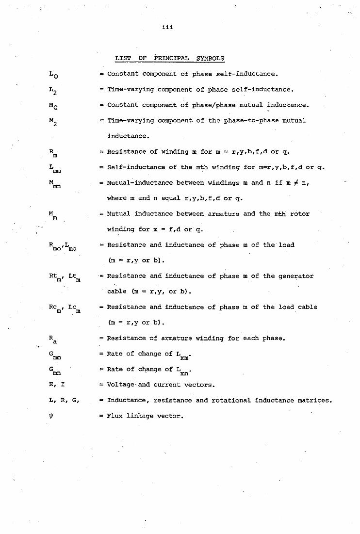
LIST OF PRINCIPAL SYMBOLS
= Constant component of phase self-inductance.
= Time-varying component of phase self-inductance.
= Constant component of phase/phase mutual inductance.
= Time-varying component of the phase-to-phase mutual
inductance.
= Resistance of winding m for m = r,y,b,f,d or q.
= Self-inductance of the m~h winding for m=r,y,b,f,d or q.
=·Mutual-inductance between windings m and n if m~ n,
where m and n equal r,y,b,f,d or q.
= Mutual inductance between armature and the mth rotor
winding for m = f,d or q.
= Resistance and inductance of phase m of the load
(m= r,y or bl.
·= Resistance and inductance of phase m of the generator
cable (m= r,y, or b).
= Resistance and inductance of phase m of the load cable
(m= r,y or b).
= Resistance of armature winding for each phase.
= Rate of change of L • mm
= Rate of change of L • mn
= Voltage·and current vectors.
= Inductance, resistance and rotational inductance matrices.
= Flux linkage vector.
i , E m m
~m
z
V max
xd
X' d
X" d
X q
X" q
X mq
xmd
xf
xkd
xkq
X· a
x2
X z
Lz
Tdo •
T' d
Tdo "
T " d
T " qo
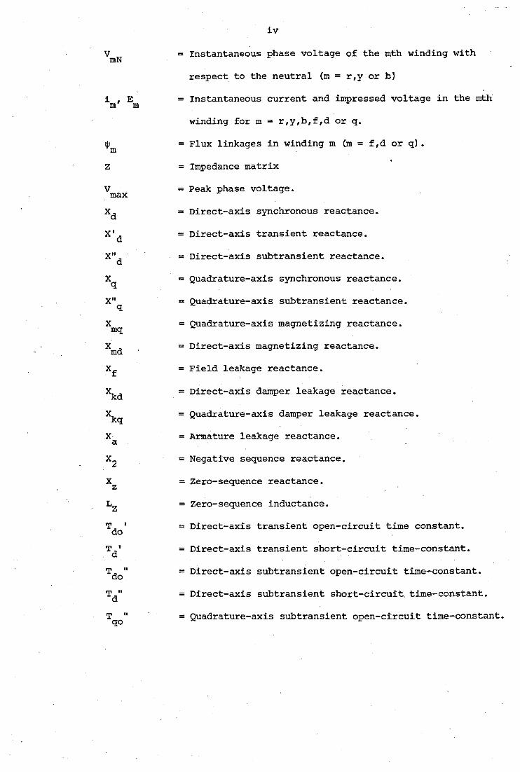
iv
= Instantaneous phase voltage of the mth winding with
respect to the neutral (m= r,y or b)
= Instantaneous current and impressed voltage in the mth
winding for m= r,y,b,f,d or q.
=Flux linkages in winding m (m= f,d or q).
= Impedance matrix
= Peak phase voltage.
= Direct-axis synchronous reactance.
= Direct-axis transient reactance.
= Direct-axis subtransient reactance.
= Quadrature-axis synchronous reactance.
= Quadrature-axis subtransient reactance.
= Quadrature-axis magnetizing reactance.
= Direct-axis magnetizing reactance.
= Field leakage reactance.
= Direct-axis damper leakage reactance.
= Quadrature-axis damper leakage reactance.
= Armature leakage reactance.
= Negative sequence reactance.
= Zero-sequence reactance.
= Zero-sequence inductance.
= Direct-axis transient open-circuit time constant.
= Direct-axis transient short-circuit time-constant.
= Direct-axis subtransient open-circuit time-constant.
= Direct-axis subtransient short-circuit. time-constant.
= Quadrature-axis subtransient open-circuit time-constant.
E , I 0 0
i me
R mm
L mm
~b G mm
E m
M
J
V
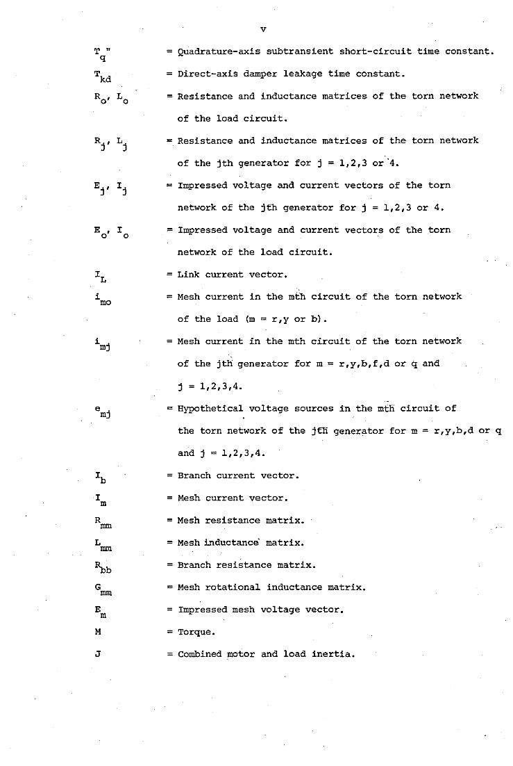
= Quadrature-axis subtransient short-circuit time constant.
= Direct-axis damper leakage time constant.
= Resistance and inductance matrices of the torn network
of the load circuit.
= Resistance and inductance matrices of the torn network
of the jth generator for j = 1,2,3 or'4.
= Impressed voltage and current vectors of the torn
network of the jtb generator for j = 1,2,3 or 4.
= Impressed voltage and current vectors of the torn
network of the load circuit.
= Link current vector.
= Mesh current in the mth circuit of the torn network
of the load (m= r,y or b).
= Mesh current in the mth circuit of the torn network
of the jth generator for m= r,y,b,f,d or q and
j = 1,2,3,4.
= Hypothetical voltage sources in the mth circuit of
the torn network of the jtli generator for m= r,y,b,d or q
and j = 1,2,3,4.
= Branch current vector.
= Mesh current vector.
= Mesh resistance matrix.
= Mesh inductance matrix.
= Branch resistance ·matrix.
= Mesh rotational inductance matrix.
= Impressed mesh voltage vector.
= Torque.
= Combined motor and load inertia.
K m
R arm
L arm
w s
w
z
Subscripts.
r,y,b
f
d
q
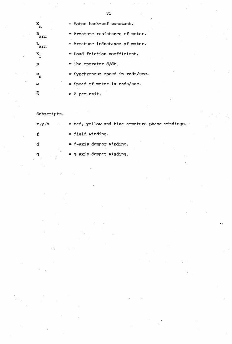
vi
= Motor back-emf constant.
= Armature resistance of motor.
= Armature inductance of motor.
= Load friction coefficient.
= The operator d/dt.
= Synchronous speed in rads/sec.
= Speed of motor in rads/sec.
= Z per-unit.
= red, yellow and blue armature phase windings.
= field winding.
= d-axis damper winding.
= q-axis damper winding.
.,
ACKNOWLEDGEMENTS
SYNOPSIS
LIST OF PRINCIPAL SYMBOLS
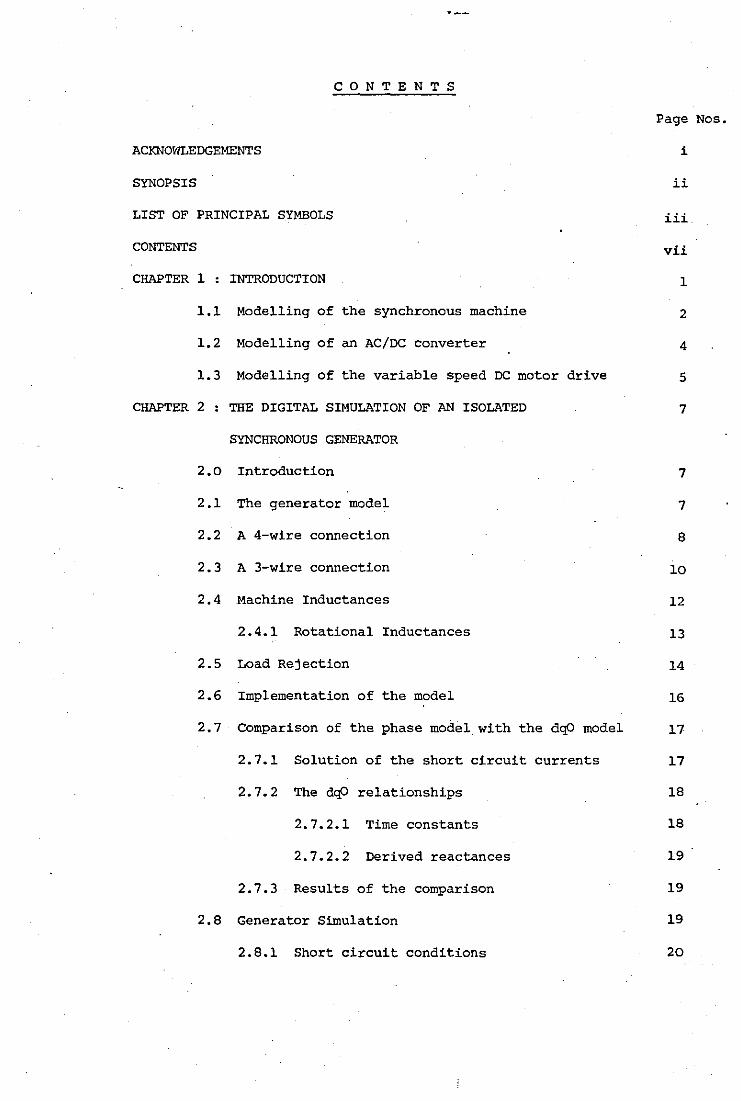
CONTENTS
CHAPTER 1 INTRODUCTION
CONTENTS
1.1 Modelling of the synchronous machine
1.2 Modelling of an AC/DC converter
1.3 Modelling of the variable speed DC motor drive
CHAPTER 2 : THE DIGITAL SIMULATION OF AN ISOLATED
SYNCHRONOUS GENERATOR
2.0 Introduction
2.1 The generator model
2.2 A 4-wire connection
2.3 A 3-wire connection
2.4 Machine Inductances
2.4.1 Rotational Inductances
Page
i
ii
iii
vii
1
2
4
5
7
7
7
8
10
12
13
2.5 Load Rejection 14
2.6 Implementation of the model 16
2. 7 Comparison of the phase model with the dqO model 17
2.7.1 Solution of the short circuit currents
2.7.2 The dqO relationships
2.7.2.1 Time constants
2.7.2.2 Derived reactances
2.7.3 Results of the comparison
2.8 Generator Simulation
2.8.1 Short circuit conditions
17
18
18
19
19
19
20
Nos.
viii
2.8.1.1 The 3-phase short circuit
2.8.1.2 Unbalanced fault situations
2.8.2 Load switching
2.8.3 Load rejection
2.9 Dqo and phase parameters of the machine
CHAPTER 3 : MODELLING OF LARGE INTERCONNECTED NETWORKS -
3.1
3.2
Analysis of a simple electric circuit
3.1.1 A diakoptic approach
3.1.2 A mesh analysis of the network
3.1. 3 Comparison of the new approach with
mesh analysis
Illustration of the diakoptic approach to a
simple multigenerator power system
3.2.1 Two generators in parallel feeding a
passive load
3.2.2 The three generator system
3.2.3 A 3-wire connection
3.2.4 Simulation of faults on the load-side
Page Nos.
20
21
21
22
22
so
51
51
54
55
56
63
65
66
3.3 Mesh analysis of a multigenerator power system 68
3.3.1 The two-generator system
3.3.2 A 3-wire connection
3.3.3 The three generator system
3.3.4 Simulation of faults on the load-side
3.4 Disadvantages of the Mesh analysis approach
3.5 Digital Simulation
69
71
72
72
73
73
3.5.1 Simulation using the Diakoptics formulation 74
3.5.2 Simulation using the Mesh analysis formulation75
3.6 Results and Discussion 76
CHAPTER 4
ix
SIMULATION OF AN AC/DC 3-PHASE FULL-WAVE
BRIDGE CONVERTER
4.1 System equations of the diode bridge model
4.1.1 The primitive reference frame
4.1.2 The mesh reference frame
4.1.3 The branch/mesh transformation
4.2 Solution process for the diode bridge model
4.2.1 Assembly of Cbm
4.2.2 Testing for discontinuities
4.2.2.1 Voltage discontinuity
4.2.2.2 Current discontinuity
4.2.3 Uncontrolled bridge simulation results
4.3 The 3-phase thyristor bridge
4.4 Computer implementation
4.4.1 The solution process
4.4.2 Discontinuity Tests
4.4.2.1 ·Turn-on
4.4.2.2 Turn-off
4.5 Controlled bridge results
CHAPTER 5 : DC MOTOR SPEED CONTROL USING A THYRISTOR CONVERTER
5.1 The system equations
5.1.1 Branch reference frame
5.1.2 Mesh reference frame
5.1.3 Branch/mesh transformation matrix
5.1.4 The complete system equations
·5.2 The computer model
5.2.1 Computer algorithm
5.2.2 Open-loop system verification
Page Nos.
111
111
112
112
114
115
116
117
117
118
118
119
121
121
122
123
123
124
·151
151
152
152
152
152
153
153
155
"
5.3
X
The closed loop system
5.3.1
5.3.2
Control system algorithm
Complete system simulation
CHAPTER 6 : CONCLUSIONS
6.1 Extension of the work for interconnected
items
REFERENCES
DqO/phase transformation
Runge-KUtta numerical integration
Page Nos.
155
157
158.
175
176
182
184
189
APPENDIX 1
APPENDIX 2
APPENDIX 3 Program Description of the 3-phase Thyristor
APPENDIX 4
APPENDIX 5
Bridge Model
The speed control circuit parameters
Listing of Computer Programs
190
193
194
1
CHAPTER 1
--·INTRODUCTION
/' Despite its theoretical abstractions, mathematical modelling has /
proved to be an invaluable aid in the design of electrical power systems,
since it enables designers to undertake detailed investigations and optimise
system parameters, prior to realization of the system. The modelling of
an electrical power system implies the prediction of both transient and
steady-state conditions in the system, adopting the most relevant and
convenient theories and techniques. Following the recent dramatic expansion
in scale and therefore complexity of power systems, a more accurate and
less time-consuming means of studying their behaviour is required than is
currently available.
The conventional mathematical approach to the solution of electrical
networks is by either a nodal or a mesh analysis. Nodal analysis involves
the formation of equations describing the network in the form Ei t=EY (Vi-V.), . ex J
whereas in mesh analysis the corresponding equations have the form
Ee = Ez(.ii-ij). In the past, these sets of equations have required much
simplification to obtain even an approximate solution, using either an
·analog or digital computer. Due to recent analytical developments and to
the present availability of powerful and high-speed digital computers,
accurate investigations of electrical networks by a numerical solution of
the full differential equations of the system are readily achieved. ·-··-
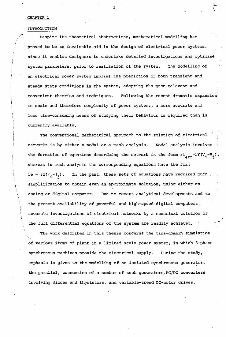
The work described in this thesis concerns the time-domain simulation
of various items of plant in a limited-scale power system, in which 3-phase
synchronous machines provide the electrical supply. During the study,
emphasis is given to the modelling of an isolated synchronous generator,
the parallel, connection of a number of such generators,AC/DC converters
involving diodes and thyristors, and variable-speed DC-motor drives.
I {
\
2
1.1 Modelling of the Synchronous Machine
The prediction of the performance of a synchronous machine has, in
the past, necessarily made use of a number of approximations, since the
solution of the system equations was laborious1 To overcome many of
these difficulties, transformations such as dqO and aSO were introduced.
2 The dqO theory was first put forward by Blonde! , and later developed by
3 4-6 Doherty and Nickle , and R.H. Park • The machine is represented by a
2-phase stationary-axis model, and the employment of various tensor
transformations enables. the time-varying coefficients present in the basic
equations to be eliminated, so as to enable an analytical solution of the
resulting equations to be made possible. Due howeve~ to various simplifying
assumptions inherent in the model, only a limited range of problems involving
balanced conditions of the generator can be easily investigated. Simulation
of the majority of unbalanced conditions the machine may encounter necessitate
a further transformation, involving either symmetrical components or an
7-10 aSO model • Although the aSO model results in differential equations
with variable coefficients, it has been found to be more convenient under
/"certain unbalanced conditions of operation10• Nevertheless, with the
present day availability of digital computers, the simulation of both
balanced and unbalanced operation based on the basic 3-phase equations
for the machine is now easily and conveniently performed, as has been
11 12 shown by many authors ' /
\
To illustrate this latter point, the modelling of an isolated 3-phase,
60 kV~,~400_~z synchronous generator using the phase reference-frame is ...-------- ·--------- ······ ····-···-·······----· discussed in Chapter 2 of the thesis.
/ The only disadvantage of the
phase model is that it involves the inversion of an inductance matrix of - --~-~--- ----------~ -----~-~-------·-···
order 5 or 6, depending on whether a 3-wire or 4-wire connection is in ----- -~- ------- -~-- -------- ---- --- . -----------.,
. use. The advantages and disadvantages of both phase and dqO reference >·---------
3
frames are discussed. The differential equations describing the model
are solved on a step-by-step basis using a fourth-order Runge-Kutta
integration technique. Various fault and load switching conditions ar~
simulated and theoretical results for a 3-phase short circuit are \ compared with the results of a classical dqO model. )
In Chapter 3 of the thesis, the isolated generator model is extended
to a parallel-connected multigenerator arrangement. A mesh or nodal
analysis becomes more complicated as additional generators are added to
the network, and the computational time required by a numerical solution
becomes increasingly significant. 13 14 However, using Kron's ' concept
of diakoptics, which involves the tearing apart of a large-scale network
into smaller sub-networks, the solution for a large network is obtained
more easily than by conventional means. In the diakoptic approach,
each sub-network is solved separately, as if it existed in isolation,
and the individual solutions are then interconnected to provide a solution
for the entire network. Provided the network has constant frequency and
correspondingly constant impedance, ananalyticalsolution for the network
may be obtained. When the network contains generators or motors the
differential equations of the system need to be integrated numerically to
obtain a solution, and the voltages at the points of tear are hence
determined iteratively. If there are too many torn networks, it is
quite possible for a numerical solution to become unstable.
The new diakoptic approach enables an exact solution for the numerical
integration of large-scale electric power networks to be obtained.
Conventional methods applied to large-scale electric power networks
containing motors or generators require a large inductance matrix to be
inverted at every stage of the solution, with the time required for this
inversion being approximately proportional to the cube of the order
4
of the matrix. However, in the new approach it is only the inductance
matrices associated with the torn networks that require to be inverted
and, since the largest of these is of order 6, a considerable saving in
computer run-time results. As the size of the original network increases,
so too does the saving in run-time, and since the large matrices of the
overall network are replaced by sub-matrices corresponding to each of
the torn networks on the leading diagonal, there is also a saving in
the core-storage required by the program.
This new approach is illustrated by applying it to a simple network
comprising two single-phase generators feeding a common passive load,
and its advantages are demonstrated by comparison with a mesh analysis
of the same network. The techniques developed are then applied to a
power system comprising 2, 3 or 4, 3-phase, 60 kVA, 400 Hz synchronous
generators connected in parallel and supplying a common bus bar, when
subjected to various fault and load switching sequences.
1.2 · Modelling of an AC/DC Converter
Although AC electric power systems are almost universally used for
large-scale"power generation and distribution, there is still a need for
conversion from AC to DC and vice-versa in HVDC transmission systems.
With the development of simple, efficient and reliable semitonductor
devices, diode/thyristor converters are commonly used.
The conventional method for solving diode and thyristor circuits
is to obtain the differential equations appropriate for every possible
change in conduction pattern, leading eventually to a large number of
differential equations which become cumbersome to handle unless the network
is simplified. However it has been shown15 that, using Kron's tensor
16 17 approach ' , a digital computer can be programmed to assemble and to
solve automatically the network equations, and this greatly reduces
5
computer run-time.
The simulation of a 3-phase full-wave diode/thyristor bridge
connected to a stiff AC supply through a cable, and supplying a passive
load, is described in Chapter 4. Kron's tensor approach is used to
assemble the relevant mesh differential equations for the changing diode/
thyristor conduction patterns and these are solved on a step~by-step
basis using numerical integration. In the simulation of th~ thyristor
bridge converter, the effect of variations in the trigger angle on the
output voltage and current waveforms is also studied.
1.3 Modelling of the Variable Speed DC Motor Drive
In the past the speed of a DC motor has typically been controlled
by means of a Ward-Leonard system, although static converters based on
18 thyratrons or mercury arc valves have also been used • During the
1960's, various important advances in the control of electrical power
took place following the introduction of the thyristor, and development
has since continued at a great pace. DC motors, combined, with thyristor
converters, provide a flexible and convenient drive system for the majority
of variable speed applications encountered within industry.
Chapter 5 describes a mathematical model for a variable speed drive,
comprising a separately-excited DC motor, with armature voltage control
provided by a 3-phase full-wave thyristor bridge. Theoretical waveforms
derived from this study are compared with corresponding waveforms obtained
on a small laboratory-scale machine. Speed control is incorporated,
and the performance of the speed control system, which controls the firing
angle by sensing the speed, current and armature power, is discussed.
Theoretical waveforms of voltage, current and speed, during steady-state
are obtained.

6
All the individual items simulated in this thesis may be interconnected
to form a typical power supply system. The thesis therefore concludes
with a brief consideration of the use of the diakoptic approach to the
simulation of a combination of all the models described previously, with
conclusions which may be drawn from the work and possible ways in which
it may be extended being discussed in Chapter 6.
The computer programs used for the simulation in Chapters. 2 and 3
were written in Fortran IV and run on an ICL 1904 computer, whilst those
used in the simulations in Chapters 4 and 5 were written in Fortran IV
(FTN77 Version) and run on a Prime computer.
7
CHAPTER 2 \
THE DIGITAL SIMULATION OF AN ISOLATED SYNCHRONOUS GENERATOR
2.0 Introduction
This chapter describes a mathematical model for an isolated 3-phase
synchronous generator with an independent voltage applied to the field
winding. The model is based on the phase reference frame, and a set of
linear differential equations with variable coefficients are presented
which describe the machine behaviour under both steady-state and transient
conditions. The model can cope with any symmetrical or asymmetrical
fault condition, load application or rejection study, for either a 3-wire
or 4-wire armature connection.
2.1 The Generator Model
The mathematical model, which consists of a set of differential
equations, can be expressed either using the dqO reference frame or the
phase reference frame. The dqO reference frame is based on Park's
definition of an ideal synchronous machine4 By making the assumptions
that speed remains constant and that there are negligible space harmonics ~---~
and no magnetic saturation in the machine, the dqO axis theory yields a
set of linear differential equations with constant coefficients, for which
an analytical solution is possible. Although the form of the equations
is simple and the solution time is short, the simulation of unbalanced
conditions is difficult to handle and a further transformation to
19 symmetrical components is necessary Transformation into a,a,o components
is an alternative in this case10•11 • /
Due to the present availability of powerful and high-speed digital ~--.--·-----------..--- .. ----------- ------ ----~ -------~----··· ----· . ----
computers, -~numeric~~- solution for the phase reference differential
equations is now feasible and no transformation is necessary. Unbalanced
faults and load switching conditions can be easily and directly simulated.
8
Higher harmonics presen~in_the air gap mmf may easily be included, as - -- -- - - -.
' -~. - - - --- ----12 is described by
1smith and Snider Although magneti_c saturation may be
included in bot~_~e!~rence frames, the inclusion of_ saturation in the phase ---reference frame is_more accurate, since each i~dividual winding __ of t~e
machin~-~an be_~~~s~~ered, whereas in the dqO reference frame, only the -- - --------------------------------~--
effect of saturation on the direct axis armature reactance is considered. --------- ...
In this thesis, saturation is neglected and only the fundamental component
of the air gap mmf wave is considered. The effects of saturation using a
12 phase reference model is discussed by some authors Saturation is
assumed on the direct axis only, and due entirely to the resultant mmf
on the direct axis. The disadvantage of a phase reference frame model -------------------------- --------- -------------
is that the time-v_aryiJ1g _ _i!1d~ctanc<3__ matrix_ needs_ to __ b: __ 1~:rertE'ld at eac~-
step of the numeric_al_solution and this could introduce long computer --- ---------~----- -~-- --. _______ .. --------·- ------ --
run-times. The disadvantage is insignificant when a high-speed digital ...-·----- --------------------- -~- -------- ---------- ------- .. ., ___________ -- -· ---,. ______ ... computer is used to obtain the solution. Parameters for the phase model
are required and since machine data is usually given in dqO form, a
dqO to phase transformation is necessary, and this is given in Appendix 1.
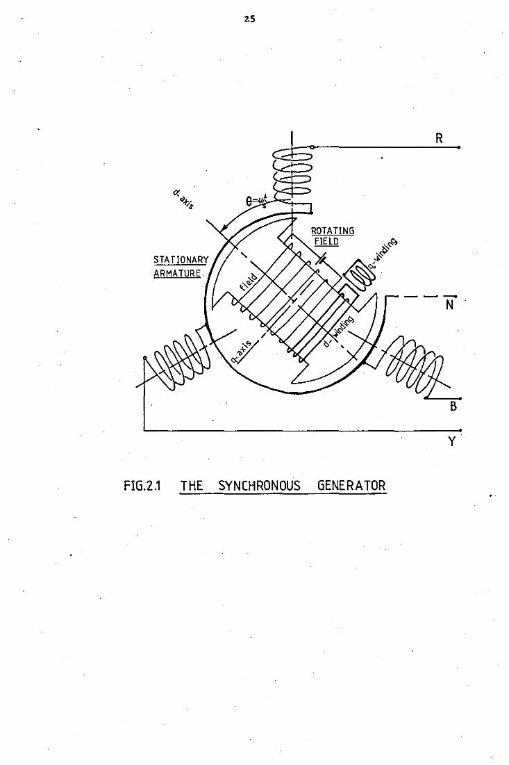
2.2 A 4-Wire Connection
A schematic representation of a synchronous generator with a 3-phase
armature winding on the stator (4-wire connection) and a salient pole (
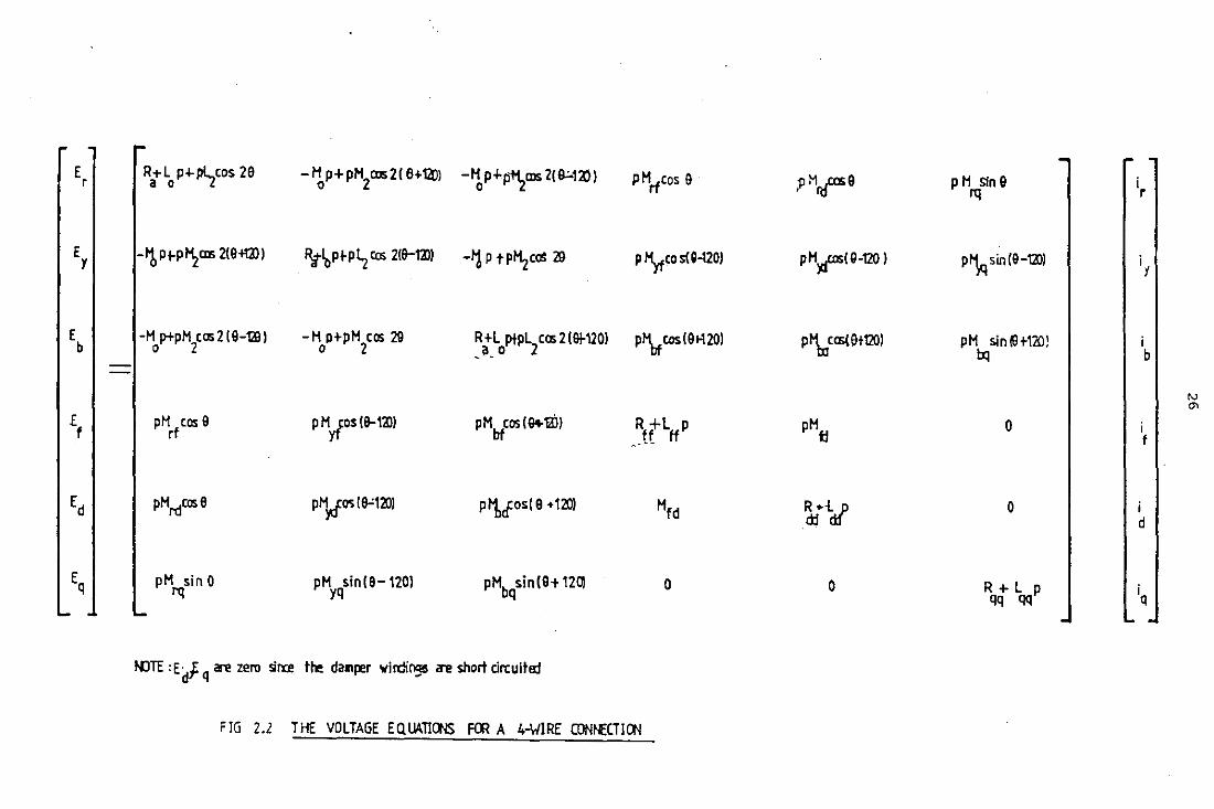
rotor with cage-type pole face damper windings is shown in Fig. 2.1.
The voltage equations describing the corresponding machine behaviour are
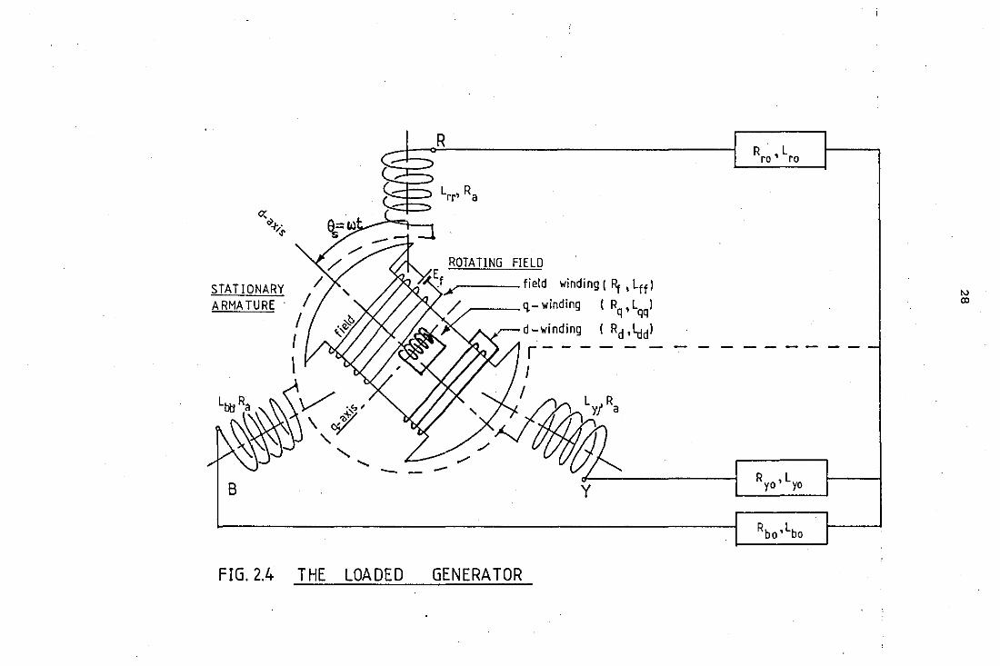
given by Fig. 2.2. When an external load consisting of a resistance R mo
and inductance L is connected in series with each phase of the armature / mo
winding m for m = r,y,b, the impedances of the individual phase windings
are modified to include the load impedances. The resistance Ra and the
self inductance of the armature windings L for m = r,y,b, are replaced mm
respectively by R and L (for m= r,y,b) where: a mm
R a
=R +R a mo
L =Lmm+L mm mo
9
for m = r,y,b
for m = r,y,b
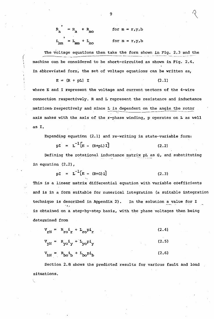
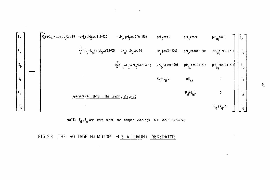
The voltage equat~ons then take the form shown in Fig. 2.3 ·and the
machine can be considered to be short-circuited as shown in Fig. 2.4.
In abbreviated form, the set of voltage equations can be written as,
E = (R + pLl I (2 .1)
where E and I represent the voltage and current vectors of the 4-wire
connection respectively. Rand L represent the resistance and inductance
matrices, respectively and since L is.dependent on the angle the rotor
axis makes with the axis of the r-phase winding, p operates on L as well
as I.
Expanding equation (2.1} and re-writing in state-variable form:
pi = 1[ . L- E - (R+pL) I] (2. 2)
Defining the rotational inductance matrix pL as G, and substituting
in equation (2.2),
pi = (2. 3}
This is a linear matrix differential equation with variable coefficients
and is in a form suitable for numerical integration (a suitable integration
technique is described in Appendix 2). In the solution a value for I .. ' is obtained on a step-by-step basis, with the phase voltages then being
determined from
vrN = R i + L . ro r ropl.r (2 .41
vyN = R i + LY0 piy yo Y (2. SJ
vbN = ~~ + ~pib (2.6}
Section 2.8 shows the predicted results for various fault and load
situations.
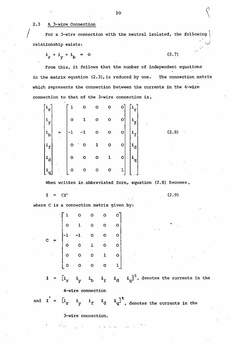
10 \. 2.3 A 3-wire Connection
I For a 3-wire connection with the neutral isolated, the following\ - / I
relationship exists: V
= 0 (2. 7)
From this, it follows that the number of independent equations
in the matrix equation (2.3),is reduced by one. The connection matrix
which represents the connection between the currents in the 4-wire
connection to that of the 3-wire connection is,
i r
i y
i q
=
1 0
0 1
-1 -1
0 0
0 0
0 0
0 0
0 0
0 0
1 0
0 1
0
0
0
0
0
0
1
i r
i y
i q
(2. 8)
When written in abbreviated form, equation (2.8) becomes,
I = CI' (2. 9)
where C is a connection matrix given by:
1 0 0 0 0
0 1 0 0 0
-1 -1 0 0 0 c =
0 0 1 0 0
0 0 0 1 0
0 0 0 0 1
I = [i i ib if id i 1t denotes the currents r y q '
4-wire connection
' =
in
[i i ]t and I i if id r y q ' denotes the currents in the
3-wire connection.
the
11
From the requirement for invariance of power, it follows that
E' = (2 .10)
where;
E' = e ]t, denotes the voltage vector in the q
3-wire connection, with erb and eyb representing the voltages
of the r and y phases taken with reference to the b phase
and E = [er ey eb ef ed. eq]t, denotes the voltage vector in
the 4-wire connection.
Then E = Z I (2 .11!
where Z is the impedance matrix in the 4-wire connection.
Combining equation (2.9) and equation (2.11)
E = Z C I'
Combining equation (2.10! and equation (2.121
et z c I' E' = ,•
(2 .12}
(2 .13)
For the 3-~ire connection, the following relationship holds,
E' = Z'I' (2. 14!
where Z' is the impedance in the 3-wire connection.
Comparison of equations (2.13) and (2.141 yields,
Z' = ctz c (2. 15)
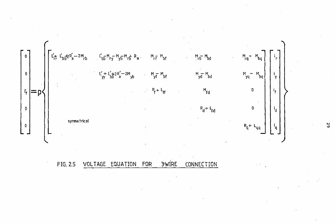
Applying the above transformation and considering the resistance and
inductance of each phase of the load combined with the corresponding
armature terms, the voltage equations take the form shown in Fig. 2.5
and the abbreviated matrix form is,
E' = (R' + PL' l I' (2 .16}
where R' and L' are the resistance and inductance matrices of a 3-wire
connection. As in section (2.2), by defining G' = pL', equation (2.16)
can be re-written,
E' = (R' + G') I' + L' pi' (2 .17)
12
Re-arranging the 3-wire equations in state-variable form, we have
' pi' = "L' ( E' - (R' + G') I' ] (2 .18)
which can be solved, using the numerical integration technique described
in Appendix 2, to arrive at the machine currents. The predicted results
for various fault and load situations are presented later in section 2.8.
2.4 Machine Inductances
(a) Self inductance of the field- and damper- windings
In the absence of stator slot effects, the self-inductances of the
field, d-axis damper and q-axis damper windings, are all independent
of the rotor position and therefore, Lff' Ldd and Lqq are constant.
(b) Rotor/rotor mutual inductances
Since the mutual inductance between the field and d-axis damper
winding is independent of rotor position, Mfd is constant. As there are
no mutual flux linkages in the q-axis winding due to the field and d-axis
damper windings, Mfq and Mdq are both zero.
(c) Stator/rotor mutual inductances
Assuming the space mmf and flux distributions are sinusoidal, the
mutual inductances between the r-phase and the rotor windings are,
Mrf = Mf cos e (2 .19) r
Mrd = Md cos e (2. 201 r
M = M sin e (2. 211 rq q r
where e is the angle the axis of the rotor makes with the axis of the r
r phase armature winding. Similar expressions for phases y and b can
0 be obtained by replacing er by er - 120
(d) Stator self-inductances.~ and e + 120°, respectively.
r
The s·elf inductances of the r-phase winding is given by
L rr = (2.22)
..
0 13 \
Corresponding expressions for L and ~b are obtained by replacing yy b
er in equation (2.22} by er - 120° and er + 120° respectively.
(e) Stator mutual inductances.
The mutual inductance between phases r and y is given by
Mry = -M0 + M2 cos 2(er + 120°} (2. 23}
Mrb and ~y are obtained by replacing er + 120° by er - 120° and
2.4.1
by e respectively. r
Rotational Inductances
Assuming the angular velocity of the rotor is ws' the various ..·
rotational inductances are as follows.
(a} Rotor self-inductances
G qq
=
=
=
0
0
0
(b) Rotor/rotor mutual inductances
(c)
= 0
Gfq = 0
Gdq = 0
Stator/rotor mutual inductances
For the r-phase,
Grf = -w· M sin e s f r
Grd = -w M sin e s d r
G = w M cos e rq s q r
Expressions for phases y and b are obtained by replacing e by r
0 0 e - 120 and e + 120 , respectively. r r .
..
14
(d) Stator self-inductances
G rr =
By replacing a by a - 120° and a + 120° respectively, G and r r r n
Gbb are obtained.
(e) Stator/stator mutual inductances
G = -2w M sin 2(e + 120°) ry s 2 r
Replacing er+ 120° by er - 120° and ar respectively, Grb and
G~ are obtained.
The inductance coefficients L0 , L2 , M0 , M2, Mf' Md and Mq used in
this section are derived in Appendix 1. The inductance matrix L and
the rotational inductance matrix G are symmetrical about their leading
diagonals. (
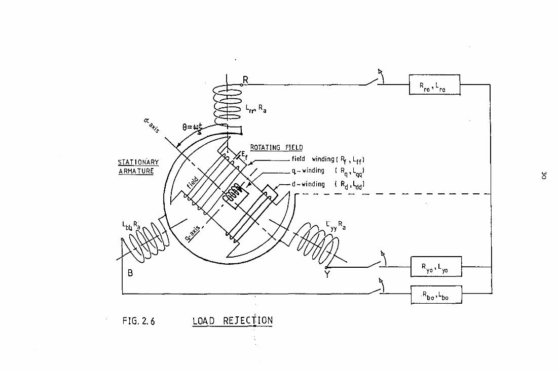
2.5 Load Rejection.
A schematic representation of the machine on load rejection is
given in Fig.~- Since i , i and ib are all zero, elimination of r Y
the rows and columns corresponding to ir' iy and ib yields the voltage
equation,
[Ef Lff
0 = Mfd
0 0 0
0
L qq i
q
l\ \ 'L' (2.24)
The initial currents on load rejection are obtained by applying the
theorem of constant flux linkages, which states that if the resistance of
a closed circuit is zero then the algebraic sum of the flux linkages
must remain constant. Since the currents in the armature windings drop
instantaneously to zero at the instant of load rejection, the currents
in the closed windings of the rotor must rise instantaneously if constant
15
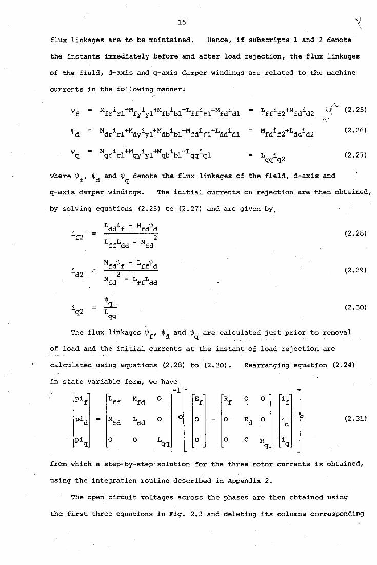
flux linkages are to be maintained. Hence, if subscripts 1 and 2 denote
the instants immediately before and after load rejection, the flux linkages
of the field, d-axis and q-axis damper windings are related to the machine
currents in the following manner:
.pf =
=
=
=
=
= L i qq q2
\..1:_/V (2. 25) f\'
(2.26)
(2.27)
where .Pf' .Pd and .Pq denote the flux linkages of the field, d-axis and
q-axis damper windings. The initial currents on rejection are then obtained,
by solving equations (2.25) to (.2.27) and are given by1
=
= .pq
L qq
(2. 28)
(2.29)
(2. 30)
The flux linkages .pf, .Pd and ljJ are calculated just prior to removal q .
of load and the initial currents at the instant of load rejection are
calculated using equations (2.28) to (2. 30) • Rearranging equation (2. 24)
in state variable form, we have -1 -
pif Lff Mfd 0 Ef Rf 0 0 if
pid = Mfd Ldd 0 0 0 Rd 0 id (2.31)
pi 0 0 L 0 0 0 R i q qq q q
from which a step-by-step solution for the three rotor currents is obtained,
using the integration routine described in Appendix 2.
The open circuit voltages across the phases are then obtained using
the first three equations in Fig. 2.3 and deleting its columns corresponding
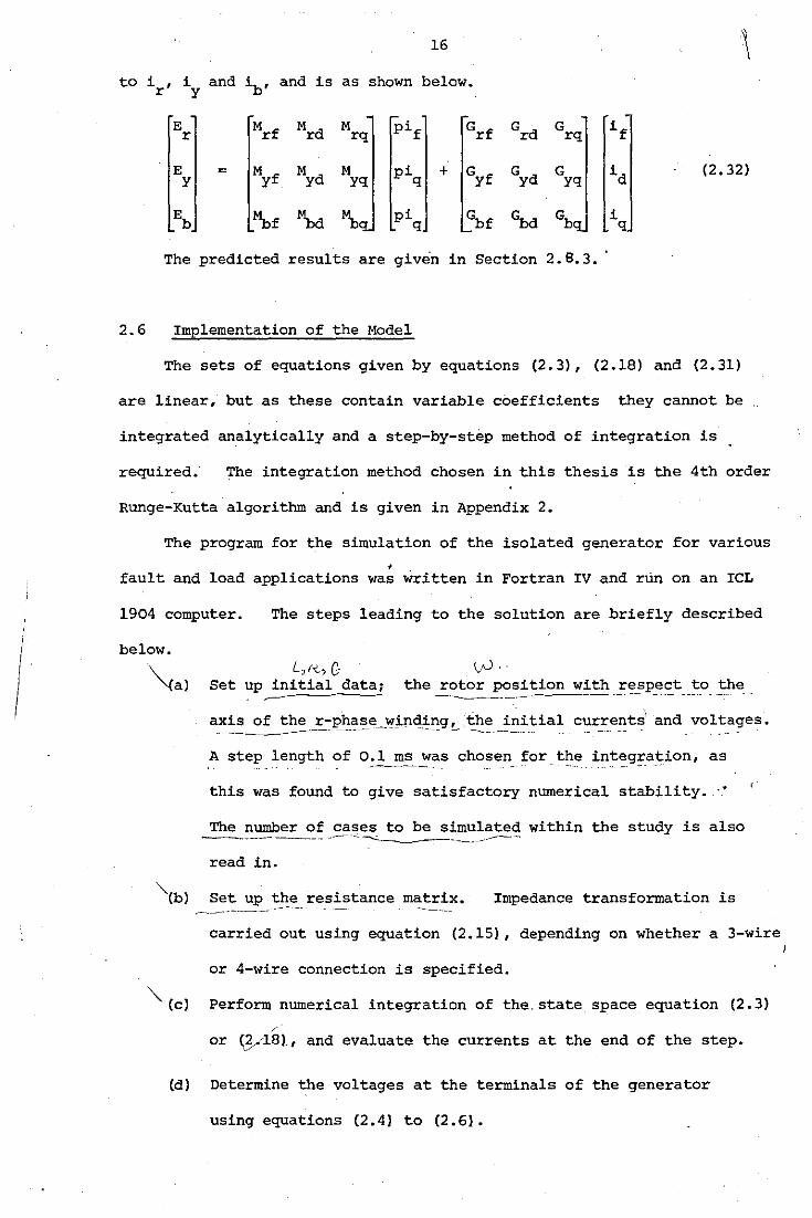
16 \ to i , i and ib' and is as shown below. r y
E Mrf Mrd M pif Grf Grd G if r rq rq
E = Myf Myd M pi + Gyf Gyd G id (2.32) y yq q yq
Eb ~f '\xi !}, pi Gbf Gbd Gb i q q
The predicted results are given in Section 2. s. 3.
2.6 Implementation of the Model
The sets of equations given by equations (2.3), (2.18) and (2.31)
are linear, but as these contain variable coefficients they cannot be
integrated analytically and a step-by-step method of integration is
required; The integration method chosen in this thesis is the 4th order
Runge-Kutta algorithm and is given in Appendix 2.
The program for the simulation of the isolated generator for various
' . fault and load applications was written in Fortran IV and run on an ICL
1904 computer. The steps leading to the solution are briefly described
below.
~a) L,r<., G vv · ·
Set up initial data; the ~osition with~r~_sp_e~t~_j:o_ the
axis of the r-phase_\ol':!.nding, the initial current~' and voltages. -~----~ ---- ----- ~ -------------
A step length of O~]:__m,:; _ __"''aS chosen for. t]l_e integ:ra:tion, as
this was found to give satisfactory numerical stability. ·•
--~-----
read in.
\b) .-------~--
Set up t~e_resistance matrix. - --~----
Impedance transformation is
carried out using equation (2.15}, depending on whether a 3-wire )
or 4-wire connection is specified.
"'-(c) Perform numerical integration of the. state space equation (2.3)
/ or ~181, and evaluate the currents at the end of the step.
(d) Determine the voltages at the terminals of the generator
using equations (2.4] to (2.6}.
17
(e) Calculations are advanced after every step, until the end of
simulation is reached. The initial currents for the next
integration step assume the values calculated at the end of the
previous step. In the case of load rejection, the initial
currents are determined using equations (2.28} to (2.30).
Proceed to step (b) for a new case, and repeat until the study
is completed. ~ \
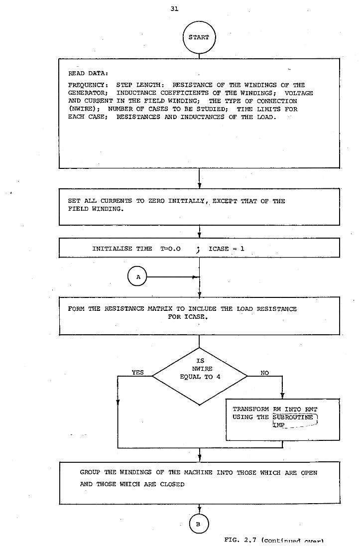
A simplified flow chart of the program is given in Fig.~
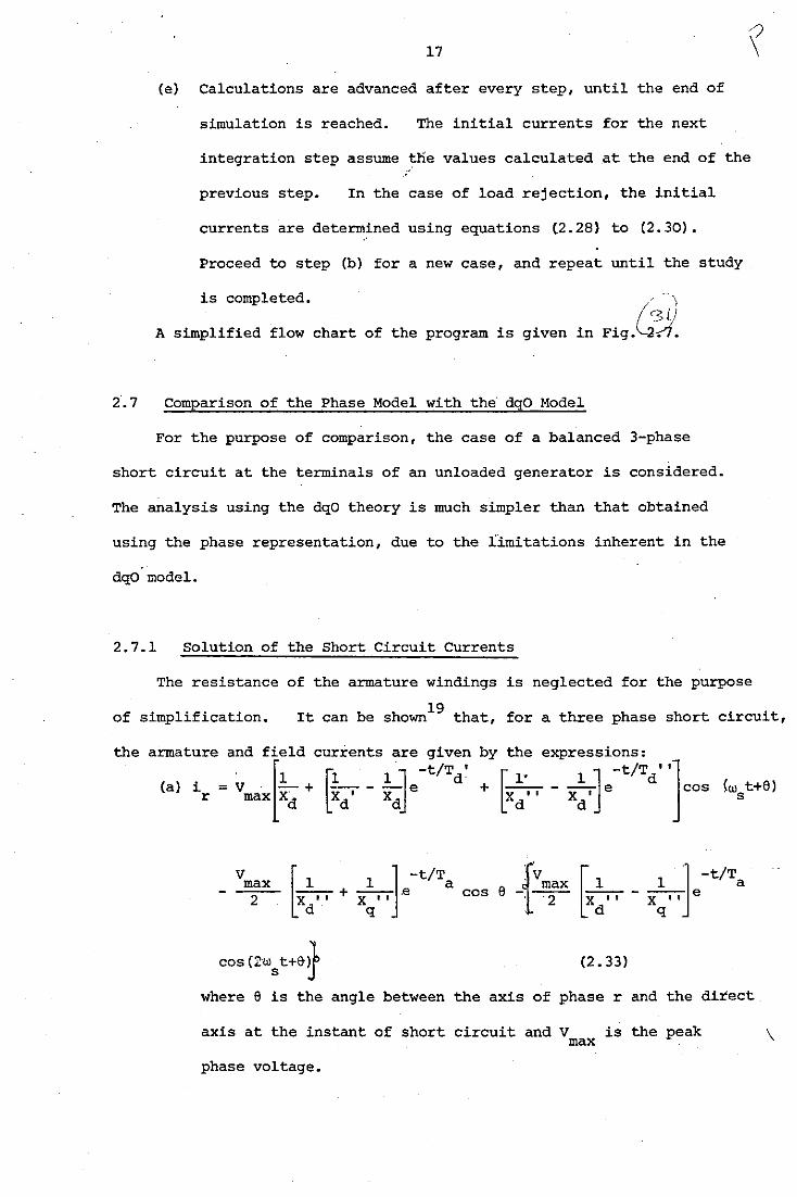
2·. 7 Comparison of the Phase Model with the dqO Model
For the purpose of comparison, the case of a balanced 3-phase
short circuit at the terminals of an unloaded generator is considered.
The analysis using the dqO theory is much simpler than that obtained
using the phase representation, due to the limitations inherent in the
dqO model.
2.7.1 Solution of the Short Circuit Currents
The resistance of the armature windings is neglected for the purpose
of simplification. 19 It can be shown that, for a three phase short circuit,
the
V max ----2
cos (l!·w s t+81 (2. 33)
(w t+8) s
where e is the angle between the axis of phase r and the direct
axis at the instant of short circuit and V is the peak \ max
phase voltage.
18
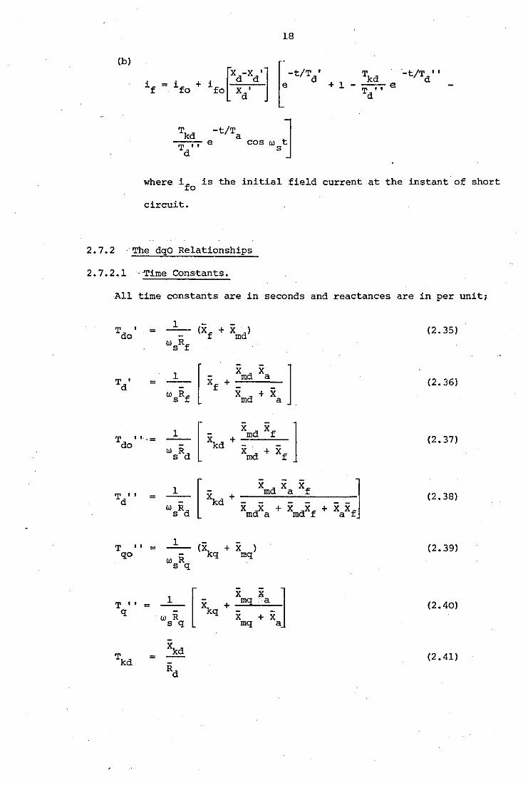
(b)
[
X -X 1
] i _d d fo X 1
d + 1 -
Tkd -t/Ta l -v- e cos w8 tj
where ifo is the initial field current at the instant of short
circuit.
2. 7. 2 -·The dqO Relationships
2. 7. 2.1 -·Time Constants.
All time constants are in seconds and reactances are in per unit;
T I
do =
T I = d
T I'··= do
T I I
d =
T ,, = qo
T I. = q
1
w R s q
1
w R s q
X mq
X mq
(2.35)
(2.36)
(2. 37)
(2. 38)
(2. 39)
(2. 40)
(2. 41)
19
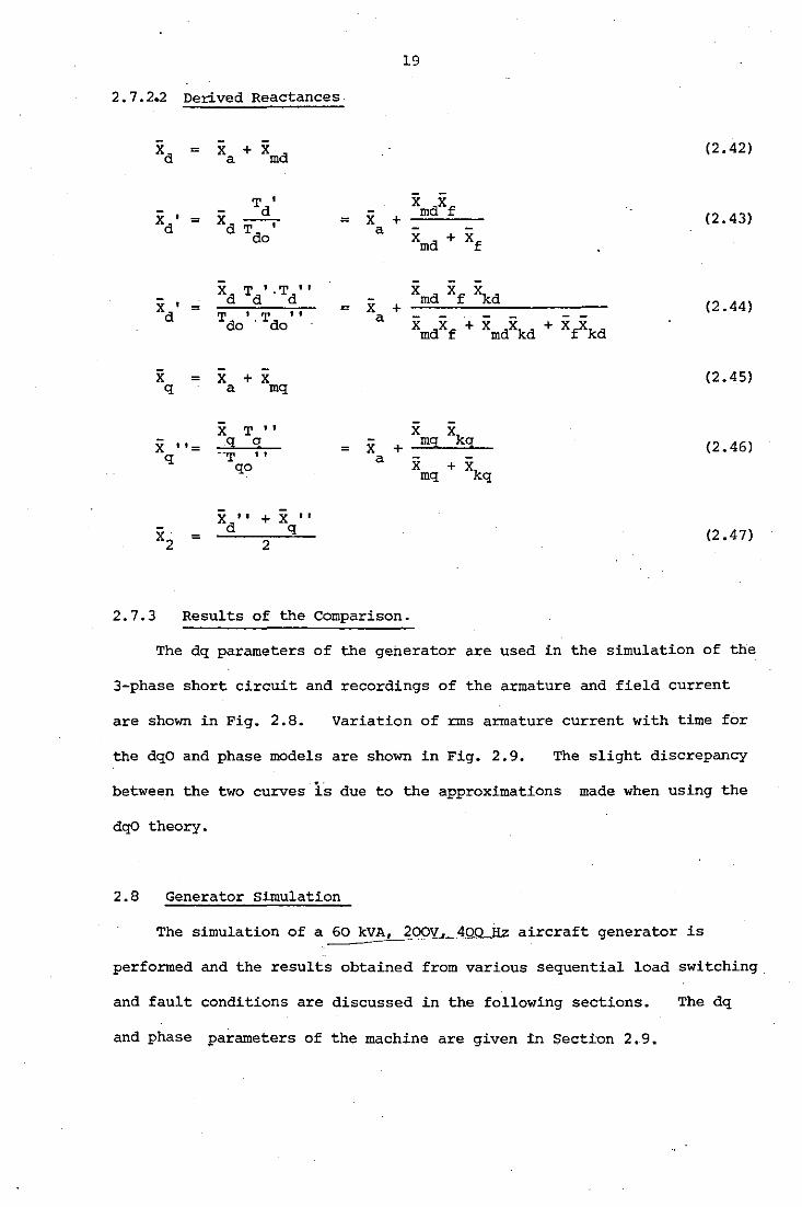
2. 7.2.2 Derived Reactances
xd = X + xmd (2.42) a
- Td I
xmdxf xd
I = xdT' = X + (2. 43) a - -do xmd + xf
xd Td I -Td I I X xf xkd
I md (2.44) xd = = X +
Tdo I
.Tdo I I a - - -
xmdxf + xmdxkd + x~kd
-X = X + X (2. 45) q a mq
X T I I X xkg; X ''= 9: 9: = X + mg; (2.46)
q .. T I I a qo X + xkq mq
xd I I + X I I
x· q (2. 4 7) = 2 2
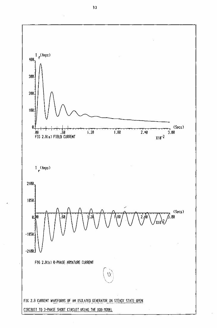
2.7.3 Results of the Comparison.
The dq parameters of the generator are used in the simulation of the
3-phase short circuit and recordings of the armature and field current
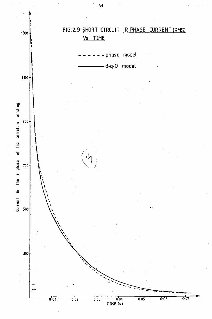
are shown in Fig. 2.8. Variation of rms armature current with time for
the dqO and phase models are shown in Fig. 2.9. The slight discrepancy
between the two curves i:s due to the approximations made when using the
dqO theory.
2.8 Generator Simulation
The simulation of a 60 kVA~_2_0QY~3.QQ.Jl;!: aircraft generator is
performed and the results obtained from various sequential load switching
and fault conditions are discussed in the following sections. The dq
and phase parameters of the machine are given in Secti'On 2 • 9.
20
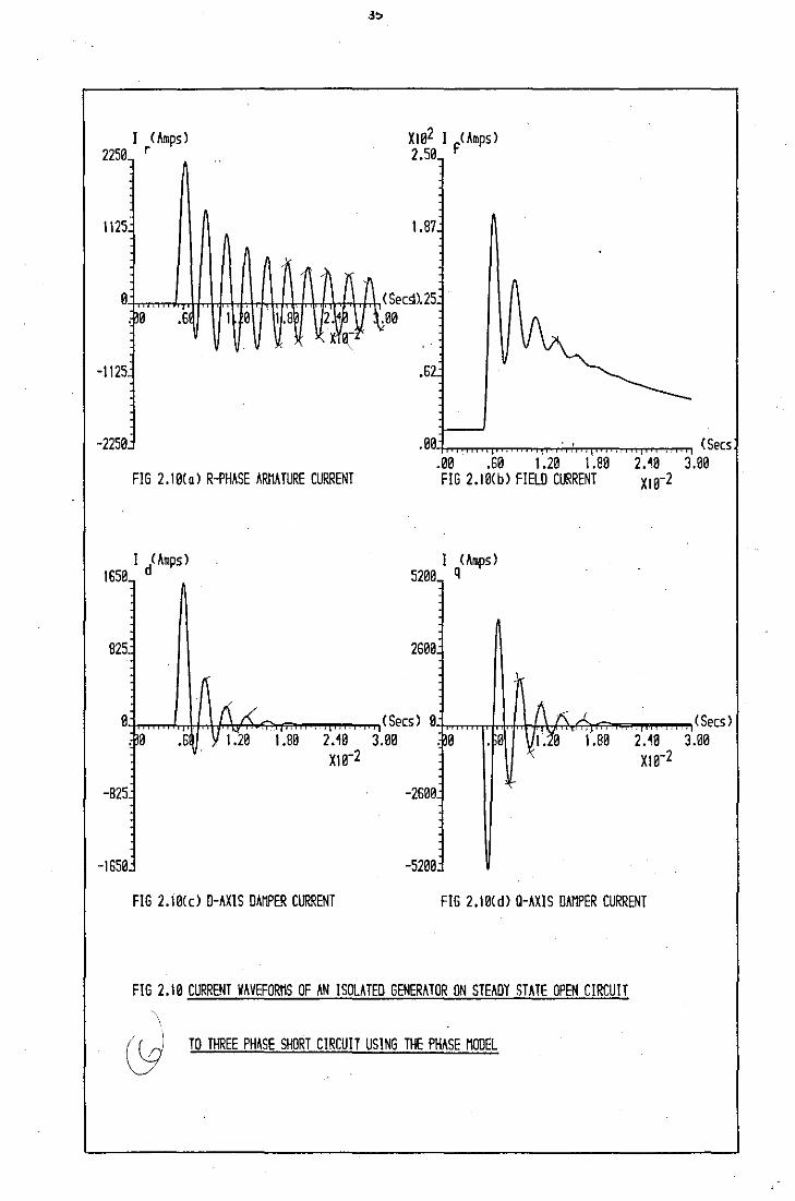
2.8.1 Short Circuit Conditions.
2.8.1.1 The 3-phase Short Circuit.
Figs. 2.iO(a), (b), (c) and (d) show the transient and steady-
state r-phase armature current and field, d-axis and q-axis damper
winding currents which follow a full-short circuit.
,c;:u>:;~;ents_are_dependent_on_the instant in th"_V£l_l_t.<•9:e_s:¥cle_ at which __ _
the.s1lOJOj;~ircuit is_~pplied, and these comprise an alternating
component of fundamental frequency, an asymmetrical component of
zero frequency and a second-harmonic component. Since the second-
harmonic component is dependent on the difference between the sub-
transient reactances of the d and q-axes, it can often be neglected,
since these reactances are very much of the same order. As seen
from Figs.2.10(a), (b), (c) and (d), the DC offset or asymmetrical
component lasts for approximately 0.018 secs. The currents in the
rotor circuits are also seen to consist of an oscillatory component
of fundamental frequency, which dies away as the DC component decays.
This is due to the DC offset component, which can be considered
frozen with' respect to the stator, inducing 400 Hz frequency currents
in the rotor as this revolves at synchronous speed. Maximum short
circuit current is obtained when the short circuit is applied at the -------·-~--- - -- --- ... -- ·- - --- ____________ , ______________ --.. --.. ------- -- - .... --- ---.------
instant the voltage passes through zero. The short circuit currents ------------are seen to decay to their sustained short circuit values due to the
weakening of the field excitation due to armature reaction. - ------------------ ·------
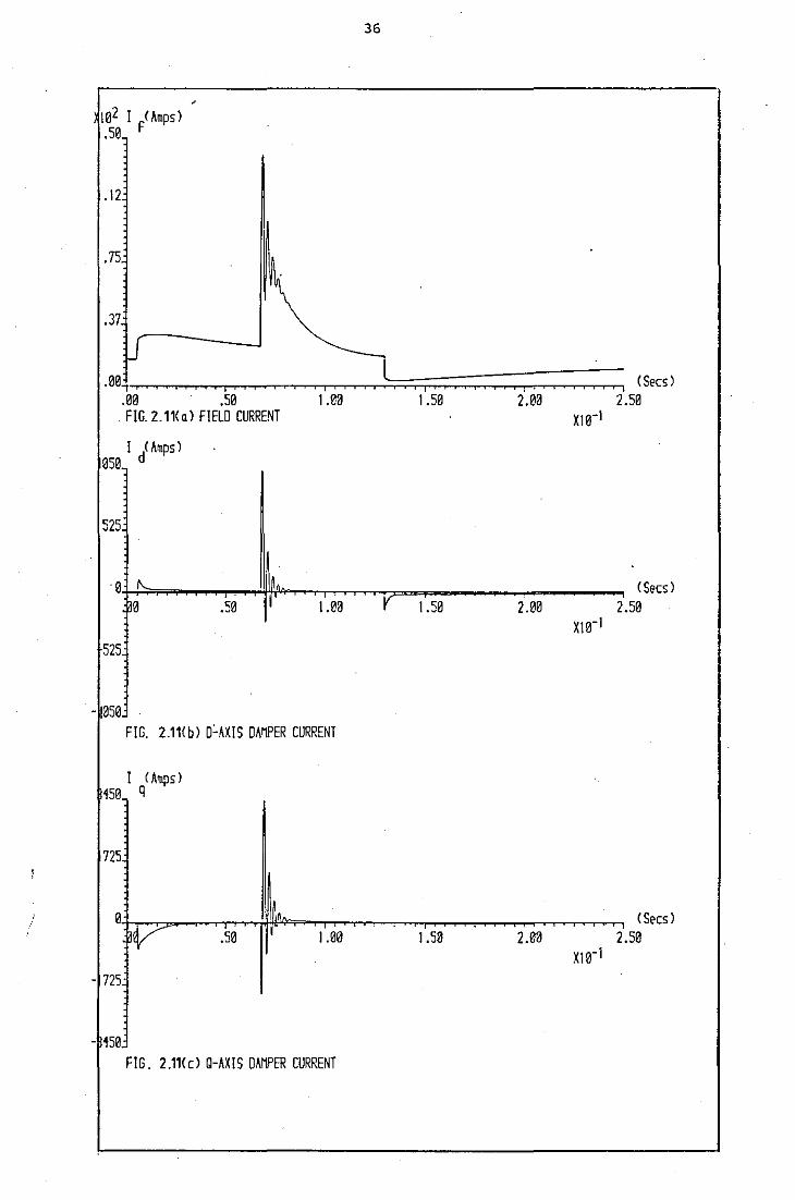
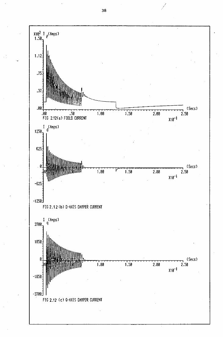
Figs. 2.11, 2.12 and 2.13 show the application of a 3-phase
short circuit following the load application, a line-to-line fault
and 2-phase to earth fault, respectively. In the case of the 3-phase
short circuit on the loaded generator (See Fig. 2.11), the initial
steady currents and voltages under loaded conditions are added to the
transient currents and voltages respectively, to determine the short
21
circuit currents of the generator. The short circuit currents
obtained for a balanced 3-phase short circuit subsequent to an initial
unbalanced fault application, are much less severe than those obtained
from loaded or no load initial condition. The reason is that the
steady-state fault currents have been achieved before the application
of the 3-phase fault.
2.8.1.2 Unbalanced Fault Situations.
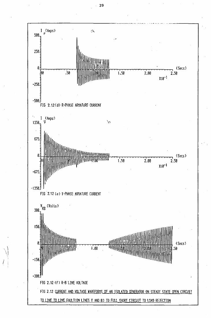
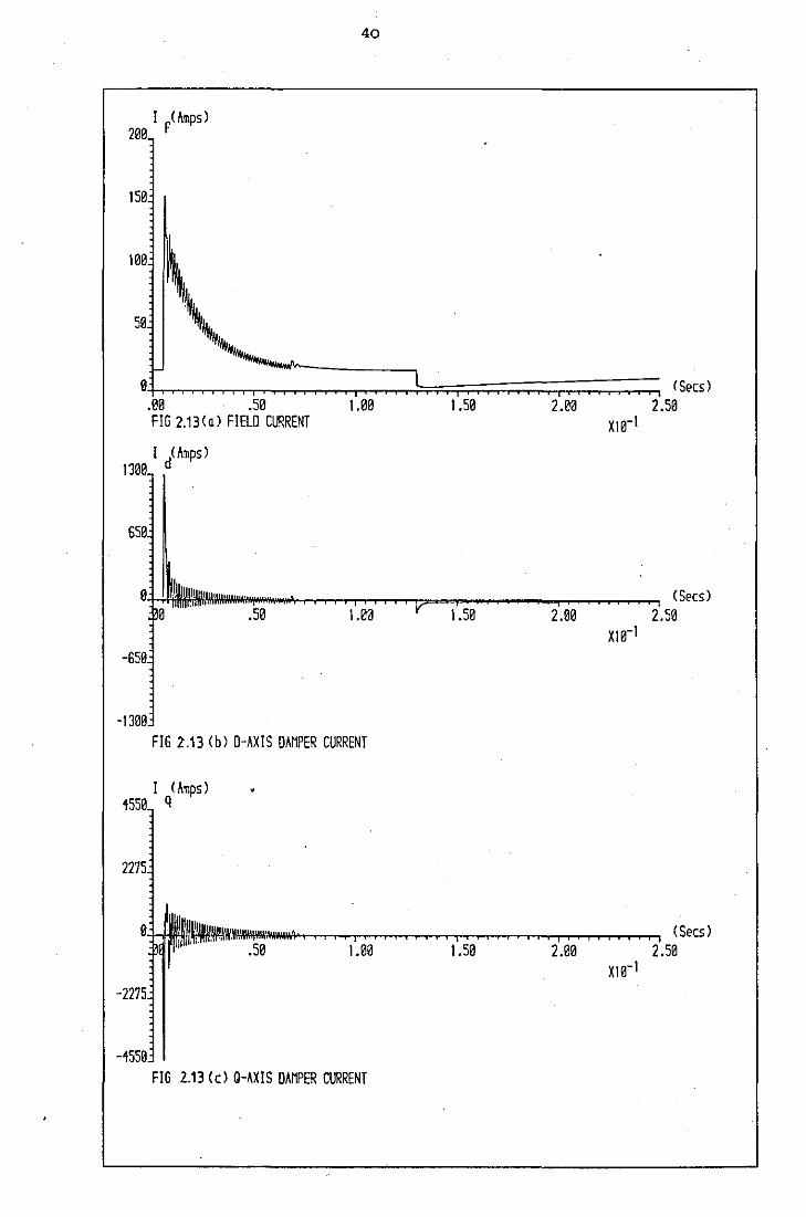
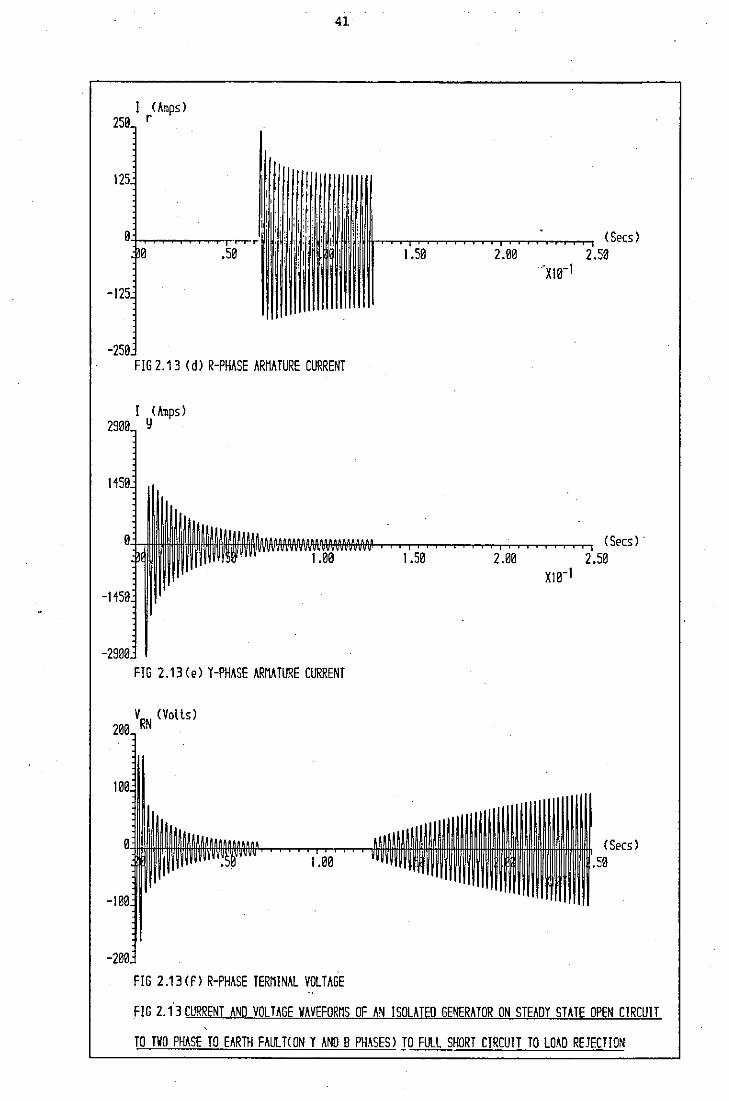
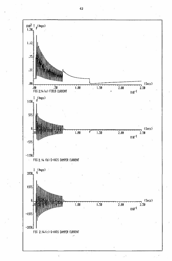
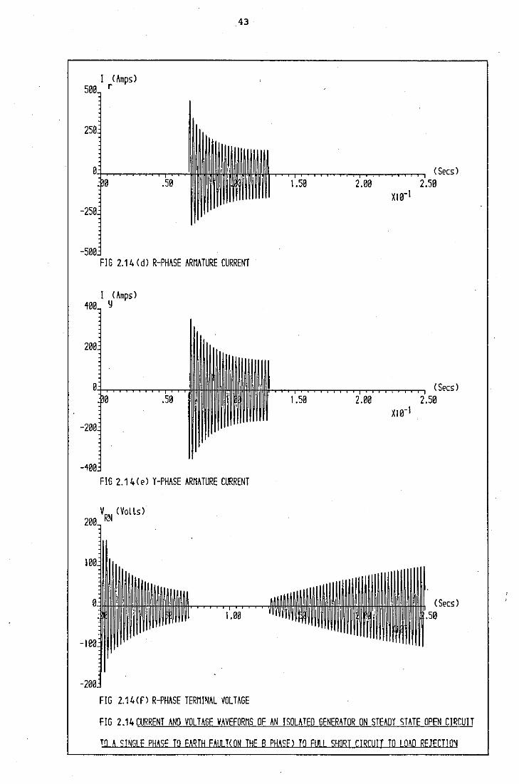
Figs. 2.12, 2.13 and 2.14 show the results obtained when a
line-to-line fault, two phase to earth,·and single phase to earth
fault are simulated, respectively. It is seen that, in the case of
the single phase to earth and the two phase to earth fault, second and
third-harmonic currents are both induced in the rotor windings,
whereas in the line-to-line simulation, no third-harmonic components
can be present, in a 3-wire connection. The presence of higher
harmonics in the unbalanced situation can be explained using the
contra-rotating field theory. Here, the unbalanced mmf of the
stator is resolved into two components, each rotating at synchronous
speed but in opposite directions. Since the rotor also rotates
at synchronous speed, second harmonic currents are induced in the
rotor, which in turn give rise to higher harmonic currents in the
machine.
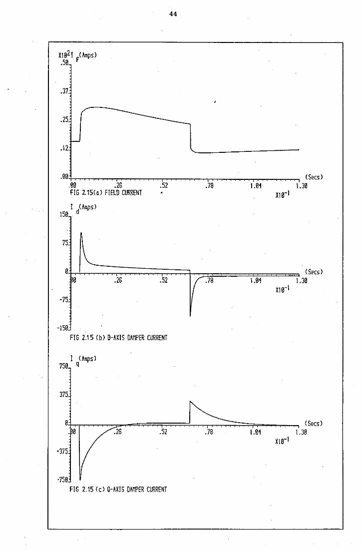
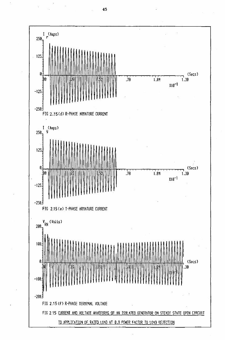
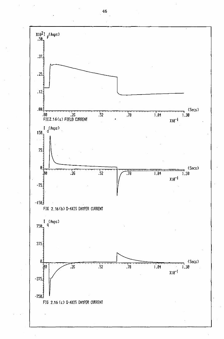
2.8.2 Load Switching.
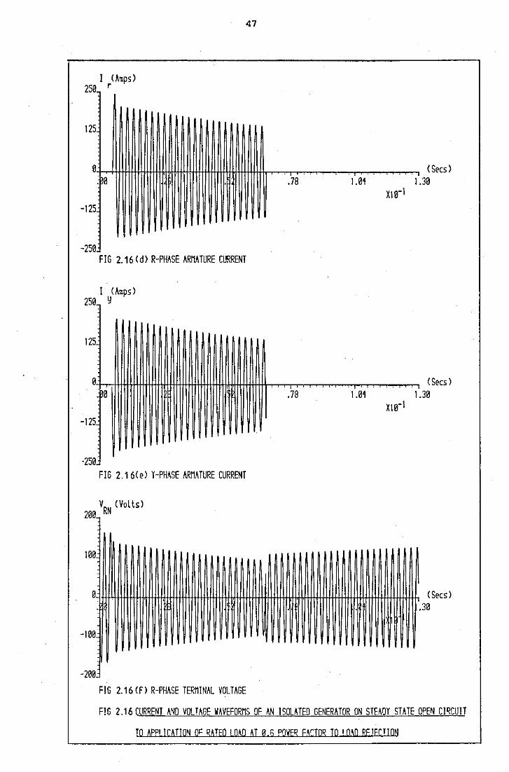
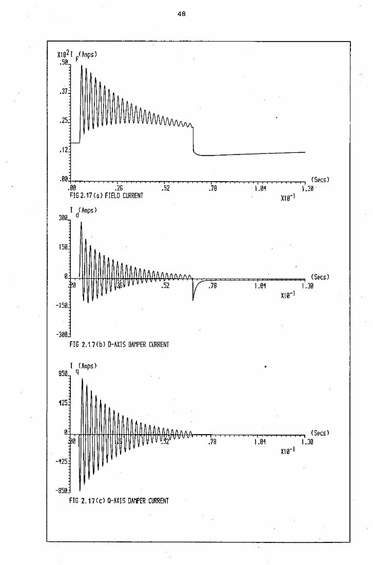
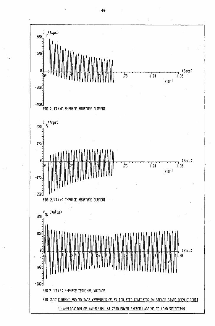
Figs. 2.15 1 2.16 and 2.17 show the currents and terminal voltages
of the machine following the sudden application of rated load at
0.8, 0.6 and zero (lagging} power factors, respectively. It is seen
that, for the case of zero power factor lag, the armature reaction'
22
is centred on the d-axis, so that no q-axis transients are present.
Since the load is very inductive, the DC component tends to decay
slowly whereas in the case of a load of 0.6 power factor or 0.8
power factor, the DC component decays quite rapidly. Oscillatory
currents of fundamental frequency are seen prominently in the zero
power factor lagging load, whereas in the case of the application
of the 0.8 power factor load, no oscillatory currents appear in the
rotor windings.
2.8.3 Load Rejection.
For the simulations considered in Figs. 2.12, 2.13, 2.14, 2.15•
2,16 and 2.17, the final simulation uses load or fault rejection.
Examination of the phase voltages or line voltages {in the case of
a 3-wire connection) indicates that,, at first, .the voltage rises
rapidly and then more slowly until the new steady value is reached.
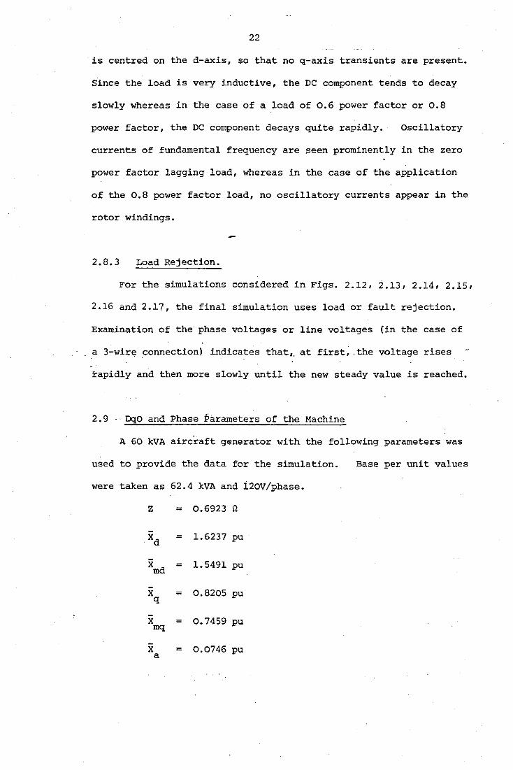
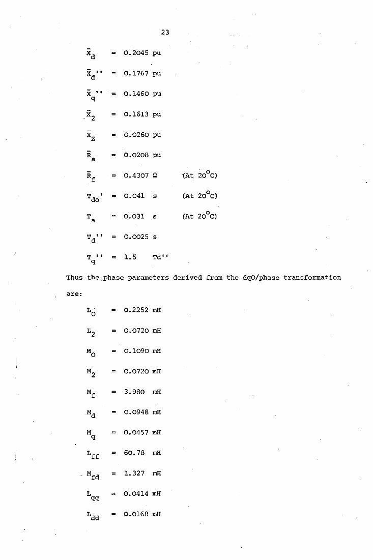
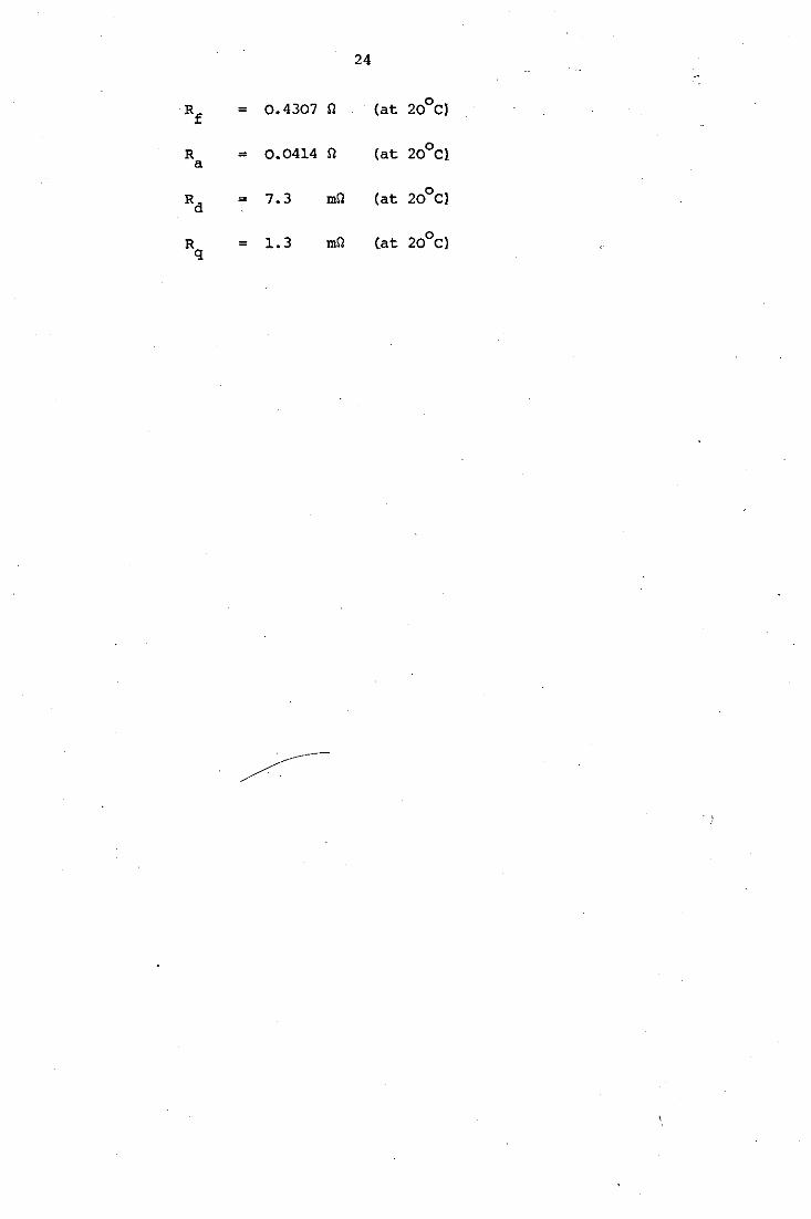
2.9 DqO and Phase Parameters of the Machine
A 60 kVA aircraft generator with the following parameters was
used to provide the data for the simulation. Base per unit values
were taken as 62.4 kVA and 120V/phase.
z = o.6923 n
xd = 1.6237 pu
xmd = 1.5491 pu
X = 0.8205 pu q
X = 0.7459 pu mq
X = 0.0746 pu a
23
xd = 0. 2045 pu
xd •• = 0.1767 pu
X •• = 0.1460 pu q
x2 = 0.1613 pu
xz = 0.0260 pu
R = 0.0208 pu a
Rf = 0.4307 Sl (At 20°C)
Tdo • = 0.041 s (At 20°C)
T = 0.031 s (At 20°C) a
Td •• = 0.0025 s
T •• = 1.5 Td 1' q
Thus the.phase parameters derived from the dqO/phase transformation
are:
Lo = 0.2252 mH
L2 = 0.0720 mH
MO = 0.1090 mH
M2 = 0.0720 mH
Mf = 3.980 mH
Md = 0.0948 mH
M = 0.0457 mH q
Lff = 60.78 mH
Mfd = l. 327 mH
L = 0.0414 mH qq
Ldd = 0.0168 mH
24
Rf = 0.4307 n (at 20°Cl
R = 0.0414 a
n (at 20°Cl
Rd = 7.3 mn (at 20°Cl
R = 1.3 q
mn (at 20°C)
2.5
R
ARMATURE
N .
B
y
FIG.2.1 THE SYNCHRONOUS GENERATOR
E r
E b
R+L p-1-DLcos 29 a o .,
-H p+pH cos2(9-t!ll 0 2
pH cos 9 rf
pH sin 0 rq
- H p+pH cos 29 0 2
pH sinl9-120) yq
Pttcfosl e +1201
I{)TE : E df q <re zero since the da11per Yirdi~ i!'l! short tircuiiB:f
FIG 2.2 THE VOLTAGE EQ~ll~ FCR A 4-WIRE CONI.ECTJ(l.l
pHr1e-120,
p~tC&(9t120)
pHtl
0 0
pH Sfn9 rq
p~sin(9-120)
0
0
R + L p qq qq
i b
I f
i d
" "'
I
Er ~+p(L0 +l_rJ+pL2Cos 29 -pM
0+Ptyos 2(!t<-120) - pM
0+pMzcos 2 ( Q -120) pMrfcos 9 pMrdcos Q pMrqsine ir
I
E R+p(L+L l + p~cos2(9-12ll - pM0+ p~cos 29 pMyfos(9 -120) pMydcos(S -120) pM sin(9-120) i y a o ye yq y
I
Eb Rtp( L0 + LtJ6+PL{os2(6+120) pM cos(9+120) pM cos(9+120) pM sin(9 +120) i
bf td bq b
< Rf+~p pMfd 0 if "f
"' ...,
Ed Rd+~dp 0 id _symmetrical ~bout the leading diagonal
Eq. R ·+L p I q qq q
NOTE: Ed , Eq are zero since the damper windi ngs are short circui ted
FIG. 2.3 THE VOLTAGE EQUATION FOR A LOADED GENERATOR
STATIONARY ARMATURE ·
R
,----field
.----- q.- winding
----B
FIG. 2.4 THE LOADED GENERATOR
R L ro' ro
y
, , , L'-M-M-M,~-R Mrf Mbf Mrb Mbd M Mbq i 0 t::+ Cbft2R -2Mb ~
rr a r bb ry yb rb a· rq r
0 t.' + t.' -HR' -2M Myf Mbf Myd Mbd M - Mbq i yy bo a yb yq y
~ =p Rf + lff Mfd 0 if
0 Rd-t- ldd 0 id
symmetrical "' 0 Rq+ lqq iq "'
FIG. 2.5 VOLT AGE EQUATION FOR 3-WIRE CONNECTION
STATIONARY ARMATURE
B
R
FIELD
..---------field winding ( ~ , Lff)
.r---- q,- winding ( Rq, Lqq)
( Rd•ludl
y
R L ro, ro
~------------------------~--------------------~~ ~~--_;--R_b_o_,L_b_o~~--~
FIG. 2. 6 LOAD REJECTION
w 0
31
-( START ) ~
READ DATA:
FREQUENCY: STEP LENGTH: RESISTANCE OF THE WINDINGS OF THE GENERATOR; INDUCTANCE COEFFICIENTS OF THE WINDINGS; VOLTAGE AND CURRENT IN THE FIELD WINDING; THE TYPE OF CONNECTION (NWIRE); NUMBER OF CASES TO BE STUDIED; TIME LIMITS FOR
EACH CASE; RESISTANCES AND INDUCTANCES OF THE LOAD.
SET ALL CURRENTS TO ZERO INITIALLY 1 . EXCEPT THAT OF THE FIELD WINDING.
~ INITIALISE TIME T=O.O . !CASE = 1 .I
A
FORM THE RESISTANCE MATRIX TO INCLUDE THE LOAD RESISTANCE FOR !CASE.
YES ~ RE NO EQUAL TO 4
TRANSFORM RM INTO RMT USING THE 'SUBROUTINE]
lMP __ - -
I
t GROuP THE WINDINGS OF THE MACHINE INTO THOSE WHICH ARE OPEN
AND THOSE WHICH ARE CLOSED
8 FIG. 2. 7 (conti nnj:lon nul:'l"t"'\
32
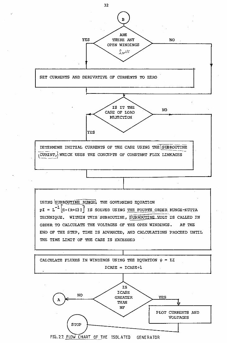
NO
SET CURRENTS AND DERIVATIVE OF CURRENTS TO ZERO
NO
DETERMINE INITIAL CURRENTS OF THE CASE USING TH~ROlJTINE
\_(:_~RIN_:J WHICH USES THE CONCEPTS OF CONSTANT FLUX LI~S
USING ~ROUTINE RU!:I~ THE GOVERNING EQUATION
pi= L-l[E-(R+G)I] IS SOLVED USING THE_~T!{_ORDERRUNGE-KU'!'TA TECHNIQUE. WITHIN THIS . SUBROUTINE, \SUBROUTINE vOLT-IS CALLED IN
ORDER TO CALCULATE THE VOLT AGES OF THE OPEN WINDINGS. AT THE
END OF THE STEP, TIME IS ADVANCED, AND CALCULATIONS PROCEED UNTIL
THE TIME LIMIT OF THE CASE IS EXCEEDED
CALCULATE FLUXES IN WINDINGS USING THE EQUATION ~ = LI
ICASE = ICASE+l
NO YES
PLOT CURRENTS AND VOLTAGES
FIG. 2.7. FLOW CHART OF THE !SOL ATED GENE RA TOR
300
200
100
0~~~~~~~~~~~~~~~~~~~~~ (Secs l 00 .60 1.20 1.80 2.10 3.00
2100
1050
FIG 2.8(al FIELD CURRENT
I (Amps) r
0 0
-1050
-2100
FIG 2.8(bl R-PHASE ARMATURE CURRENT
FIG 2.8 ~URRENT WAVEFORMS OF AN ISOLATED_GEN~R~O~~N STEADY STATE OPE~
CIRCIUIT TO 3-PHASE ~HORT CIRCUIT USING THE OQO MODEL
x10-2
<Secs) .00
en c: '0 c: :0 .. ,_ " ~ "' E ,_ "' .. "" ~ -0
.. "' "' "" a. ,_
.. "" ~ c:
~
c: .. ,_ ,_ " u
• ' ' I 1300 I
1100
900
700
500
300
~ \ I I
0·01
34
FIG. 2;9 SHORT CIRCUIT R PHASE CURRENT (RMSl
Vs TIME
- - - - - - phase model
---- d~q-0 model
/
(
\\ I
t7j \, ' I
'" /
' ... " .... ....
'
----0·02 0·03 0·04 0·05 0·06 0·07
TIME (s)
I <Amps) 2250 r
1125
0 . 0 .6
-1125_
-2250
1 0
1.87
11 (Sec~l.25
1.8 2 .. !j v0 X I(L
.6
.00 . .00 .60 1.20 1.80
FIG 2.10(a) R-PHASE ARMATURE CURRENT FIG 2.10(b) FIELD CURRENT
I iAmpsl 1650
825
I <Amps) 5200 q
2600
(Secs 2.'10 3.00 Xl0-2
0'-j,-.,~l,.,..l.tnt,fr.'ry'rl.<?rf;,.,.,.,........,.,..,.,..,.,...,.,< Secs) 0-f,.,.,~,-/ro!Hn'l-+.\oMAF.>o....,...,..,.,..,.,..., <Secs) . 0 .6 1.80 2.'10 3.00 . 0 . 0 2.'10 3.00
x10-2 x10-2
-825 -2600
-1650 -5200
FIG 2.10(c) D-AXIS DAMPER CURRENT FIG 2.10(d) Q-AXIS DAMPER CURRENT
FIG 2.10 CURRENT WAVEFORMS OF AN ISOLATED GENERATOR ON STEADY STATE OPEN CIRCUIT
TO THREE PHASE SHORT CIRCUIT USING THE PHASE MODEL
36
' 102 I F(hmps) .50
.12
.75
.37
w .00, (Secs)
.00 .50 1.00 1.50 2.00 2.50 FIG.2.11(a) FIELD CURRENT X\0-1
050 1 ihmpsl
525
0 r-. I~, (Secs l 0 .50 1.00 V 1.50 2.00 2.50
X\0-1
525
- 050_ FIG. 2.11(b) D~AXIS DAMPER CURRENT
1 (Amps) 450 q
725
; 0 t (Secs l av .50 1·.00 1.50 2.00 {sa X\0-1
- 725
- 150 FIG. 2.11(c) Q-AXIS DAMPER CURRENT
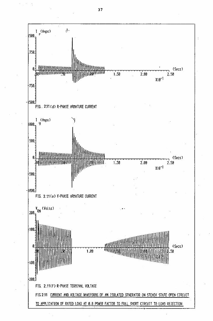
I <A~psl r
FIG. 2.11 ( e l r -PHASE ARMATURE CURRENT
1.00
FIG. 2.11<fl R-PHASE TERMINAL VOLTAGE
37
1.50
1.50
2.00
.00
(Secs l 2.50
(Secs l .50
<Secs l
FIG.2j1 CURRENT ANO VOLTAGE WAVEFORMS OF AN ISOLATED GENERATOR ON STEADT STATE OPEN CIRCUIT
38
1.00 FIG 2.12(a) FIELD CURRENT
1.00
FIG 2.12 (b) D-AXIS DAMPER CURRENT
.00
FIG 2.12 (cl Q-AXIS DAMPER CURRENT
1.50
1.50
.50
2.00
.00
(Secs) .50
(Secs l .50
(Secs) .50
~------------------------------------------------------~
·-. \ \I
I
39
...------------------------------ ------- .. ---.-- ··-·
I (Amps) r
FIG 2.12 (d) R-PHASE ARMATURE CURRENT
FIG 2.12 (e) Y-PH~SE ARMATURE CURRENT
1.00
FIG 2.12 <Fl R-8 LINE VOLTAGE
I I I I
1.50 2.00
' 1.50 .00
••
(Secs) 50
(Secs l
FIG 2.12 CURRENT 6NO VOLTAGE VAVEFORMS OF AN ISOL6TEO GENERATOR ON STEADY STATE OPEN CIRCUIT
TO LINE TO LINE FAULT( ON LINES Y AND Bl TO FULL SHORT CIRCUIT TO LOAD REJECTION
I F(Amps) 200
150
100
50 \
40
~--01~~~~~~~~~~~~~~~ <Secs) .00 .50 1.00 FIG 2.13(a) FIELD CURRENT
u ' ' I I
.50
FIG 2.13 (b) D-AXIS DAMPER CURRENT
I <Amps) q
1.00
FIG 2.13 (c) a-AXIS DAMPER CURRENT
1.50
.50
1.50
2.00 2.50 X10⁻¹
2.00
(Secs) I
.50
(Secs) 2.50
41
I (Amps) r
FIG 2. 13 ( d) R-PHASE ARMATURE CURRENT
FIG 2.13(e) Y-PHASE ARMATURE CURRENT
1.00
FIG 2.13(f) R-PHASE TERMINAL VOLTAGE
1.50 2.00
1.50 2.00
(Secs) 2.50
(Secs)·
(Secs> .50
FIG 2.13 CURRENT AND VOLTAGE WAVEFORMS OF AN ISOLHEO GENERATOR ON STEADY STATE OPEN CIRCUIT
TO TWO PHASE TO EARTH FAULT< ON Y AND B PHASES) JO FULL SHORT CIRCUIT TO LOAD REJECTION
42
.00 .50 1.00 1.50 FIG 2..14(a) FIELD CURRENT
I d(Amps)
1.00 1.50
FIG 2.14 Cbl D-AXIS DAMPER CURRENT
1.00 .50
FIG 2.14(c) 0-AXIS DAMPER CURRENT
43
I <Amps) r
FIG 2.14 ( d l R-PHASE ARMATURE CURRENT
.50
FIG 2. 1 4 ( e l Y -PHASE ARMATURE CURRENT
1.00
FIG 2.14(f) R-PHASE TERMINAL VOLTAGE
1.50
1.50
(Secs l .50
(Secs) .50
(Secs) .50
FIG 2.14CURRENT AND VOLTAGE WAVEFORMS OF AN ISOLATED GENERATOR ON STEADY STATE OPEN CIRCUIT
TO A SING! E PHASE TO EASTH FAin I< ON THE B PHASE> TO FUlL SHORT CIRCUIT TO LOW REJECITON
44
.37
.25
.12
.001.:t-,-~~~T"T"T~~~.,...-~~~___,-~~~,....,~~~..,....,..., (Secs) .00 .26 .52 .78 1.01 1.30 FIG 2. 15( a) FIELD CURRENT Xl0-l
150 I iAmps)
75
eb-L::_::;;::;:::;::;:;::;:~::;::;::;:;:::r::::='~===~:;====;> <Secs> 0 .26 .52 . 78 1.01 1.30
-75
-150 FIG 2.15 (b) 0-AXIS DAMPER CURRENT
l (Amps) 750 q
375
-375
·750 FIG 2.15 (c) Q-AX!S DAMPER CURRENT
45
I <Amps) 250 r
125
0 (Secs) 0 .78 1.0i 1.30
X10-1
-125
-250 FIG:2;1S<d> R-PHASE ARMATURE CURRENT
I (Amps) 250 y
125
0 (Secs) .. 1'.30 ·0 .78 1.01
m-1
-125
-250 FIG 2.15 (e) HHASE ARMATURE CURRENT
200 VRN (Volls)
100
0 (Secs) . ' .30
-100_
-200
FIG 2.15 (f) R-PHASE TERMINAL VOLTAGE
FIG 2.15 CURRENT AND VOLTAGE WAVEFORMS OF AN ISOLATED GENERATOR ON STEADY STATE OPEN CIRCUIT
TQ ~PE!IC~T!ON OF RATED L0\0 AT 0.8 POWER FACTOR TO L0\0 REJECTION
46
X102 I F( Amps l .50
.37
.25 --
.12
.00 (Secs l - ' '
.s2 ' '
.00 .26 .78 1.01 1.30 FIGZ.16(a) FIELD CURRENT . m-1
150 I iAmpsl .
75
0 <Secs l 0 .26
' '~
.78 1.01 1.30 .52 x10-1
-75
-150 FIG 2. 16(bl D-AXIS DAMPER CURRENT
I (Amps) 750 q
375
0 (Secs l
7.26
' ' '
'1·.30 0 .52 .78 1.01 x1e-1
-375
-750 FIG 2_16 (cl Q-AXIS DAMPER CURRENT
47
I (Amps) 250 r
125
0 (Secs) : 0 ·.'7a 1.01 1°.30
x10-1
-125
-250 FIG 2.16 (d) R-PHASE ARMATURE CURRENT
I (Amps) 250 y
125
0 (Secs) ... 0 . 78 1.01 1.30
x10-1
-125,
·250 FIG 2. 1 6 ( e l Y -PHASE ARMATURE CURRENT
200 VRN <Volts)
100,
0 (Secs) . .30
-100
-200,
FIG 2.16 (f) R-PHASE TERMINAL VOLTAGE
FIG 2.16CURRENT AND VOLTAGE WAVEFORMS OF AN ISOLATED GENERATOR ON STEADY STATE OPEN CIRCUIT
TO ~EPI IC~TIQ~ o~ 8~IED LO~D ~I a.S EO~ER E~riOS IQ !OlD ~ETECIIO~
48
.00'.:f-..~~~ ......... ~~~~.,...,.~~~,....,..,~~~~.,...~~~........, (Secs) .00 .26 .52 .78 1.04 1.30 FIG 2.17 (a l FIELD CURRENT
300 I d( Amps l
150
-150
-300 FIG 2.17(bl D-AXIS DAMPER CURRENT
I (Amps) 850 q
425
-425
-850 FIG 2.17(cl Q-AXIS DAMPER CURRENT
49
I (Amps) 100 r
200
0 (Secs l 0 .78 1'.01 1.30
m-1 ' -200
-100 FIG 2. 17 ( d l R-PHASE ARMATURE CURRENT
I <Amps> 350 y
175
0 (Secs l 0 .78 1.01 1.30
m-1 -175
-350 FIG 2.17Cel Y-PHASE ARMATURE CURRENT
200 VRN (Volts)
100
0 (Secs) .30
I
-100
-200 FIG 2.17CPl R-PHASE TERMINAL VOLTAGE
FIG 2.17 CURRENT AND VOLTAGE WAVEFORMS OF AN ISOLATED GENERATOR ON STEADY ST~TE OPEN CIRCUIT
TO APPLICATION OF RATED LOAD AT ZERO POWER FACTOR LAGGING TO LOAD REJECTION
50
CHAPTER 3
MODELLING OF LARGE INTERCONNECTED NETWORKS
The formation and solution of the sets of equations describing
a large network using mesh analysis results in an excessive computational
time. However, an alternative approach using diakoptics was introduced
13 by Kron , and this has been found to offer many advantages. The
approach involves the tearing of the large-scale electrical network into
' an appropriate number of smaller networks, with these being solved
individually as if each existed alone, and the solutions then being
interconnected to obtain a solution for the entire network. Iterative
techniques are necessary for a numerical solution, to solve for the
voltages at the points of tear, and these must be identical on both sides
of the tear. 14 In this chapter a new approach is discussed, which
enables an exact solution to be obtained for any number of torn
networks. The point of tear is always arbitrary, and for convenience
each torn network can be made to comprise an item of plant from the
network, thereby enabling the separate study of an identifiable item.
The solution of a network containing generators yields time-
v~rying inductance matrices, which require the ·inversion of a· large
inductance matrix at every stage of the solution, with the solution
time required being approximately proportional to the cube of the
matrix order. In a diakoptic approach, it is the much smaller
matrices associated with the torn networks that require inversion,
thereby resulting in a considerable saving in computer run-time.
As the size of the original network increases, so too does the saving
brought about by the new approach, a feature which is illustrated by
considerations of several multigenerator power systems.
51
3.1 Analysis of a Simple Electrical Circuit.
3.1.1 A diakoptic approach.
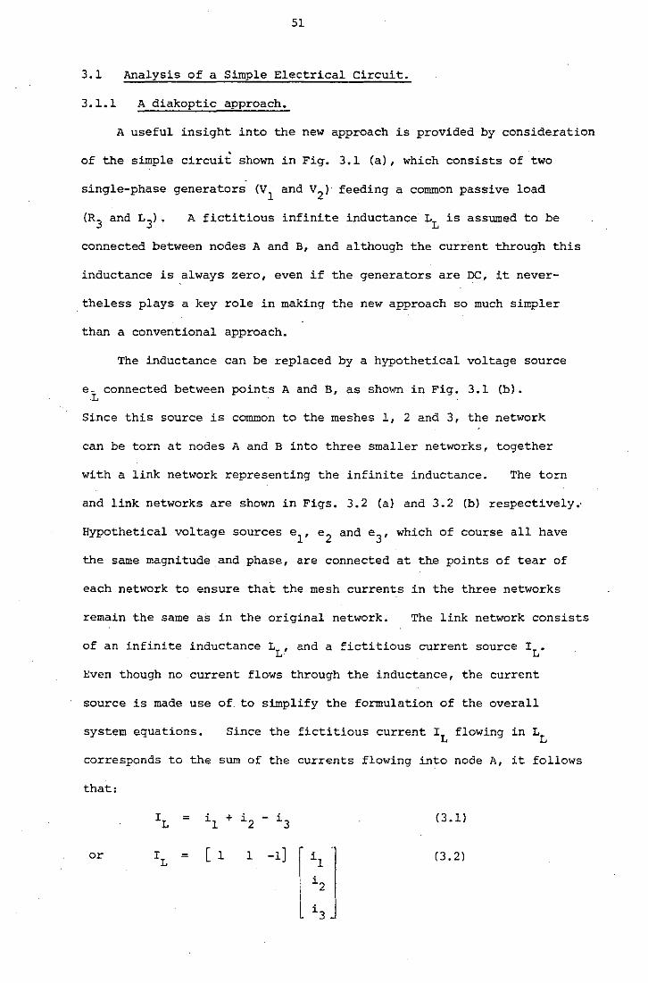
A useful insight into the new approach is provided by consideration
of the simple circuit shown in Fig. 3.1 (a), which consists of two
single-phase generators cv1
and v2 ) feeding a common passive load
A fictitious infinite inductance LL is assumed to be
connected between nodes A and B, and although the current through this
inductance is always zero, even if the generators are DC, it never-
. theless plays a key role in making the new approach so much simpler
than a conventional approach.
The inductance can be replaced by a hypothetical voltage source
e .. connected between points A and B, as shown in Fig. 3.1 (b) • . L
Since this source is common to the meshes 1, 2 and 3, the network
can be torn at nodes A and B into three smaller networks, together
with a link network representing the infinite inductance. The torn
and link networks are shown in Figs. 3.2 (a) and 3.2 (b) respectively.·
Hypothetical voltage sources e1
, e2
and e3
, which of course all have
the same magnitude and phase, are connected at the points of tear of
each network to ensure that the mesh currents in the three networks
remain the same as in the original network. The link network consists
of an infinite inductance LL, and a fictitious current source IL.
Even though no current flows through the inductance, the current
source is made use of. to simplify the formulation of the overall
system equations. Since the fictitious current IL flowing in LL
corresponds to the sum of the currents flm<ing into node A, it follows
that:
IL = il + i2 - i (3 .1) 3
or IL = [ 1 1 -1] r
il (3. 2)
I i2
l i3 J
52
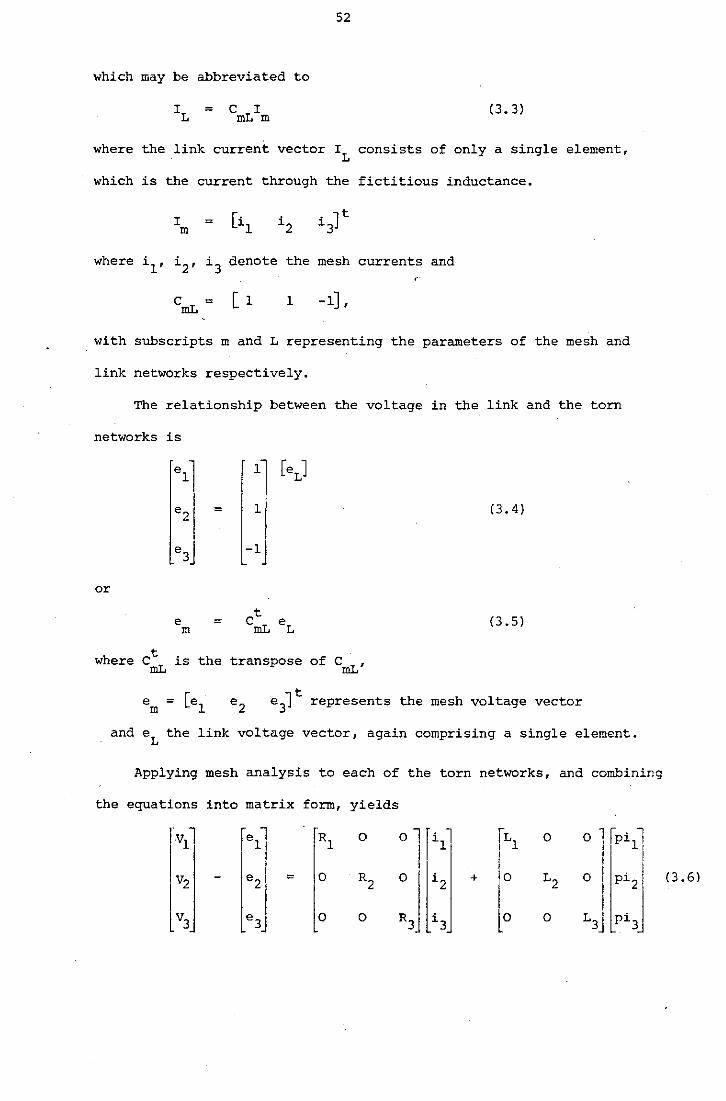
which may be abbreviated to
where
which
where
=
the link
e I mLm
current vector IL
is the current through the
I [il i2 . Jt = ].3 m
il, i2, i3 denote the mesh
emL = [ 1 1 -1],
( 3. 3)
consists of only a single element,
fictitious inductance.
currents and ,.
with subscripts m and.L representing the parameters of the mesh and
link networks respectively.
The relationship between the voltage in the link and the torn
networks is
e1l 1 [eL]
e2 = 1 (3. 4)
e3J -1
or
e = et eL m mL (3.5)
where et mL
is the transpose of emL,
e 3lt represents the mesh voltage vector
and eL the link voltage vector, again comprising a single element.
Applying mesh analysis to each of the torn networks, and combining
the equations into matrix form, yields
lv1 el rR1 0
0 l rill ILl 0 o l fPill
j l' e2 = 0 R2
0 l'' + 0 L2 0 pi2 v2
c, ,j v3 e3 0 0 R3j i3 0 0
(3. 6)
53
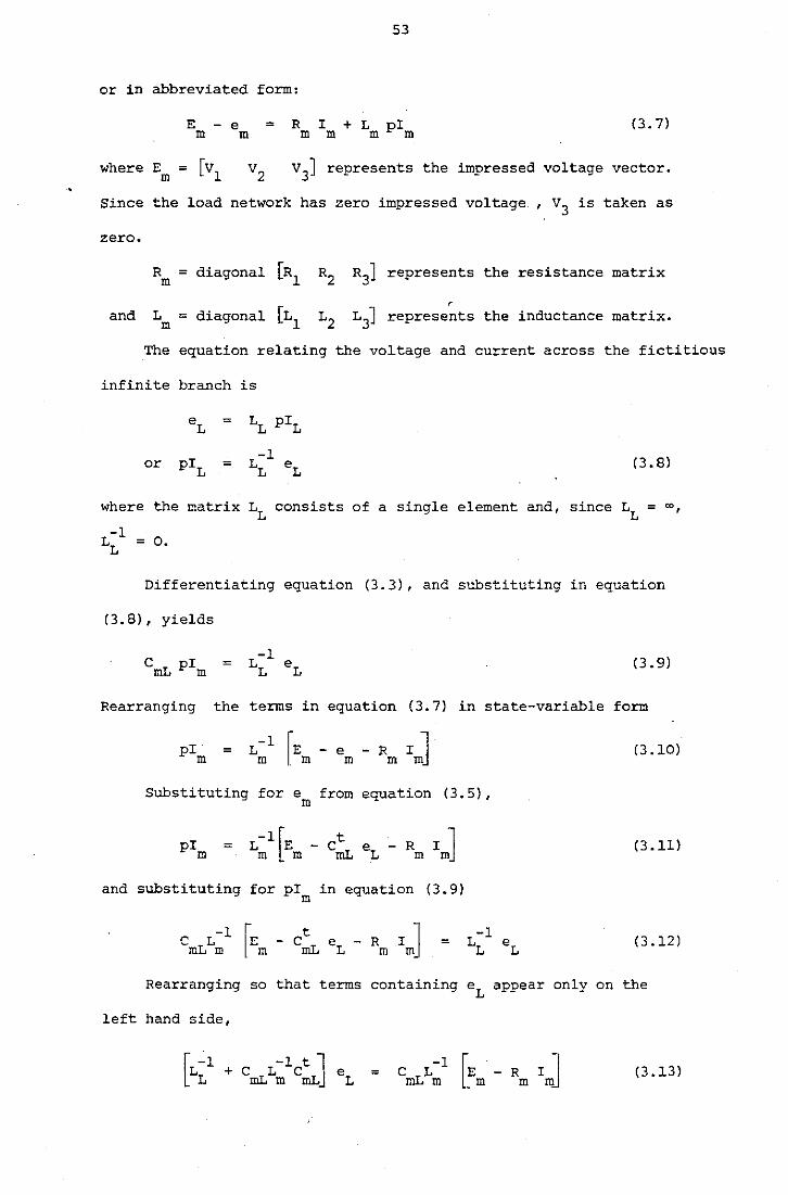
or in abbreviated form:
E - e = R I + L pi m m m m m m
(3. 7)
v3
] represents the impressed voltage vector.
Since the load network has zero impressed voltage. , v3
is taken as
zero.
Rm = diagonal [R1
R2
R3
] represents the resistance matrix
and L = diagonal [Ll Lz m L
3] represents the inductance matrix.
The equation relating the voltage and current across the fictitious
infinite branch is
eL LL piL
or piL = -1
LL eL (3. 8)
where the matrix LL consists of a single element and, since LL = m,
-1 LL = 0.
Differentiating equation (3.3), and substituting in equation
(3.8), yields
(3. 9)
Rearranging the terms in equation (3.7) in state-variable form
pi = L-l rE - e - R ImJ m m I. m m m
Substituting fore from equation (3.5), m
and substituting for pi in equation (3.9) m
C LL-1 ~E m m lj m
- et e -mL L R I J m m
=
(3.10)
(3 .11)
( 3 .12)
Rearranging so that terms containing eL appear only on the
left hand side,
= R m
(3.13)
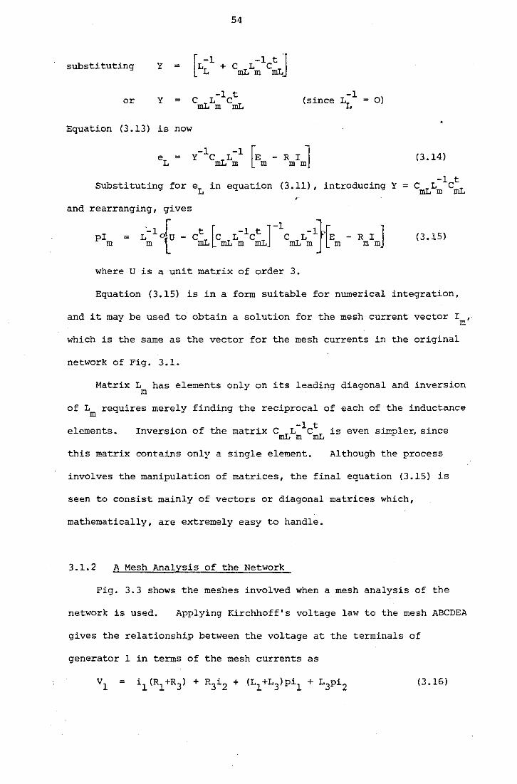
54
substituting y = [ -1 -1 t J LL + CmLLm CmL
or y = -1 t
CmLLm cmL (since -1
LL 0)
Equation (3.13) is now
Substituting for eL in equation (3.11), introducing Y
and rearranging, gives
pi m
= ~:l+ - c~[cmLL:1c~r\mLL:l}rEm where u is a unit matrix of order 3.
- R I ]mm
(3.14)
( 3.15)
Equation (3.15) is in a form suitable for numerical integration,
and it may be used to obtain a solution for the mesh current vector I , m
which is the same as the vector for the mesh currents in the original
network of Fig. 3.1.
Matrix L has elements only on its leading diagonal and inversion m
of L requires merely finding the reciprocal of each of the inductance m
elements. -1 t
Inversion of the matrix CmLLm cmL is even simple4 since
this matrix contains only a single element. Although the process
involves the manipulation of matrices, the final equation (3.15) is
seen to consist mainly of vectors or diagonal matrices which,
mathematically, are extremely easy to handle.
3.1. 2 A Mesh Analysis of the Network
Fig. 3.3 shows the meshes involved when a mesh analysis of the
network is used. Applying Kirchhoff's voltage law to the mesh ABCDEA
gives the relationship between the voltage at the terminals of
generator 1 in terms of the mesh currents as
= (3.16)
55
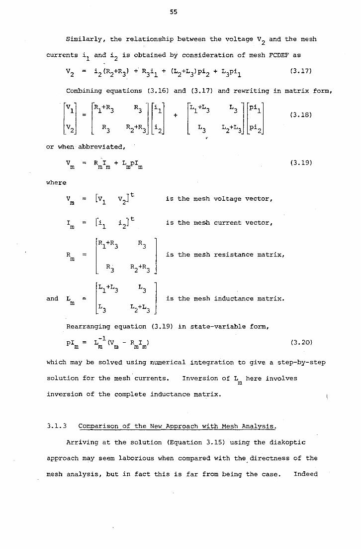
Similarly, the relationship between the voltage v2
and the mesh
currents i 1 and i 2 is obtained by consideration of mesh FCDEF as
= (3 .17)
Combining equations (3.16) and (3.17) and rewriting in matrix form,
+ ( 3. 18)
or when abbreviated,
V = R I + L pi m m m m m
(3 .19)
where
V = [vl v2Jt m is the mesh voltage vector,
I = Ci1 m 0 ]t '-2 is the mesh current vectOr,
Rl+R3 R3
l R = m
R3 R2+R3
is the mesh resistance matrix,
I., .. , L3
I and L = m
L3 L2+L3 is the mesh inductance matrix.
Rearranging equation (3.19) in state-variable form,
pi = L -l (V - R I ) m m m m m
( 3. 20)
which may be solved using numerical .integration to give a step-by-step
solution for the mesh currents. Inversion of L here involves m
inversion of the complete inductance matrix.
3.1. 3 Comoarison of the New Aooroach with Mesh Analysis.
Arriving at the solution (Equation 3.15) using the diakoptic
approach may seem laborious when compared with the. directness of the
mesh analysis, but in fact this is far from being the case. Indeed
56
its advantage is seen increasingly as the system becomes larger.
Comparison of the inductance matrices in the two methods indicates
that a diagonal matrix is obtained in the diakoptic approach, resulting
in a simpler inversion and requiring less computer time. Whatever
the size of the network, the inductance matrix will always consist of
block diagonal matrices so that, for inversion of the inductance
matrix, only submatrices are inverted •• In mesh analysis the inductance
matrix contains non-zero off-diagonal elements, which implies that the
whole matrix has to be inverted. For the small network considered,
this would cause no major problem, since the inductance matrix is only
of order 2, but inversion of the inductance matrix for a larger network
will take an appreciable amount of computing time. More core storage
too will be required to store all the elements of the inductance matrix.
3.2 Illustration of the Diakoptic Approach to a Simple Multigenerator
Power System
The first situation considered is that of a limited power-supply
system, comprising two 3-phase synchronous generators connected
in parallel and supplying a passive load through a short transmission
line. The study is subsequently extended to the case when additional
generators are present. The generators and the load are modelled
individually, and then combined to form a model for the complete
system. The modifications introduced by the presence of balanced and
unbalanced load-side faults are also discussed.
3.2.1 Two Generators in Parallel Feeding a Passive Load
The power system is shown schematically in Fig. 3.4. Each
synchronous generator has a 3-phase armature winding on the stator,
,,
together with field, d-axis damper and q-axis damper windings on
the salient-pole rotor. It is assumed that the generators are driven
at constant speed and that a constant voltage is supplied to the
field of each generator.
Fictitious infinite inductances Lk, L~ and Lm are connected
respectively between points R-N, Y-N and B-N of Fig. 3.4. The network
is then torn apart from the generator bus bars, to form the three
small torn networks and three link networks shown in Fig. 3.5. The
torn networks represent the three items of the network, namely the
two generators and the load. Hypothetical voltage sources e ., e ., rJ YJ
ebj (for j=l,2) for the generators and ero' eyo' ebo for the load are
connected across the points of tear for the torn networks formed by
generators 1,2 and the load, respectively. The magnitude and sense
of these voltages is such that the mesh currents in the torn networks
are the same as those in the original network.
Since the magnitudes of the fictitious current sources (ik, i~,
i ) in the link networks are equal to the sum of the currents flowing m
into nodes R, Y and B respectively, it follows that
ik = -i - i + i rl r2 ro ( 3. 21)
i~ = -i - i + i yl y2 yo
( 3. 22)
i -ibl -m ib2 + ibo (3. 23)
where irj' iyj and ibj (for j=l,2) denote the mesh currents in the
armature of the jth generator and iro' iyo' ibo' the mesh currents
in the load network.
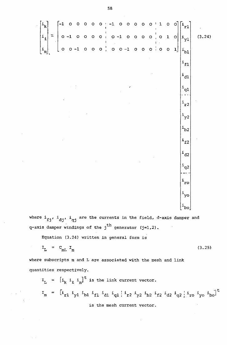
Expressing in matrix form the link currents in terms of the
mesh currents, we obtain
ik -1 0 0 0 0 0 '
i~ :: 0 -1 0 0 0 0 '
i 0 0 -1 0 0 0 m
58
-1 0 0 0 0 0 I
0 -1 0 0 0 0
0 0 -1 0 0 0
1 0
0 1
0 0
0
0
1
irl
iyl
ibl
ifl
idl
iql
ir2
iy2
ib2
if2
id2
iq2
i ro
l~yo ~bo
(3.24)
where ifj' idj' iqj are the currents in the field, d-axis damper and
q-axis damper ~indings of the jth generator {j=l,2).
Equation (3.24) written in general form is
= {3. 25)
where subscripts m and L are associated with the mesh and link
quantities respectively.
= [ik i~ im]t is the link current vector.
is the mesh current vector.
59
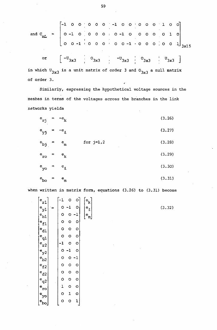
[-: 0 0 0 0 0 -1 0 0 0 0 0 1 0
:L and cmL = -1 0 0 0 0 0 -1 0 0 0 0 0 1
0 -1 ' 0 0 0 0 0 -1 0 0 0 0 0
or [ -u3x3 03x3 -u3x3 03x3 u3x3 ]
in which u3x3 is a unit matrix of order 3 and 0 3x3 a null matrix
of order 3. '
Similarly, expressing the hypothetical voltage sources in the
meshes in terms of the voltages across the branches in the link
networks yields
e = -ek (3.26) rj
e = -et (3.27) yj
ebj = e m
for j=l,2 (3.28)
e = ek (3.29) ro
e = et (3.30) yo
ebo = e (3. 31) m
when written in matrix form, equations (3.26) to (3.31) become
er1l -1 0 0
[~i ey1 = 0 -1 0 (3.32)
eb1 0 0 -1
efl 0 0 0
ed1 0 0 0
eq1 0 0 0
er2 -1 0 0
ey2 0 -1 0
eb2 0 0 -1
ef2 0 0 0
ed2 0 0 0
eq2 0 0 0
e 1 0 0 ro e 0 1 0 yo
ebo 0 0 1
60
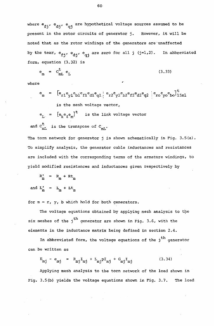
where efj' edj' eqj are hypothetical voltage sources assumed to be
present in the rotor circuits of generator j, However, it will be
noted that as the rotor windings of the generators are·unaffected
by the tear, efj' edj' eqj are zero for all j (j=l,2).
form, equation (3.32) is
where
e = m
=
et mL eL
'
is the mesh voltage vector,
is the link voltage vector
and c~ is the transpose of cmL.
In abbreviated
(3.33)
The torn network for generator j is shown schematically in Fig. 3.5(a).
To simplify analysis, the generator cable inductances and resistances
are included with the corresponding terms of the armature windings, to
yield modified resistances and inductances given respectively by
R' = R + Rt m m m
and L' = L + Lt m m m
for m = r, y, b which hold for both generators.
The voltage equations obtained by applying mesh analysis to t~e
th . six meshes of the j generator are shown in Fig. 3.6, with the
elements in the inductance matrix being defined in section 2.4.
In abbreviated form, the voltage equations of the jth generator
can be written as
= (3.34)
Applying mesh analysis to the torn network of the load shown in
Fig. 3.5(b) yields the voltage equations shown in Fig. 3.7. The load
61
impedances in the three phases are combined with the load cable
impedances to give the modified load impedances.
R' = R + Re mo mo m
and L' = L +Le mo me m
for m = r, y, b.
In abbreviated form, the voltage equations for the load network can
be written·
r E - e = R I + L pi
0 0 00 0 0 (3. 35)
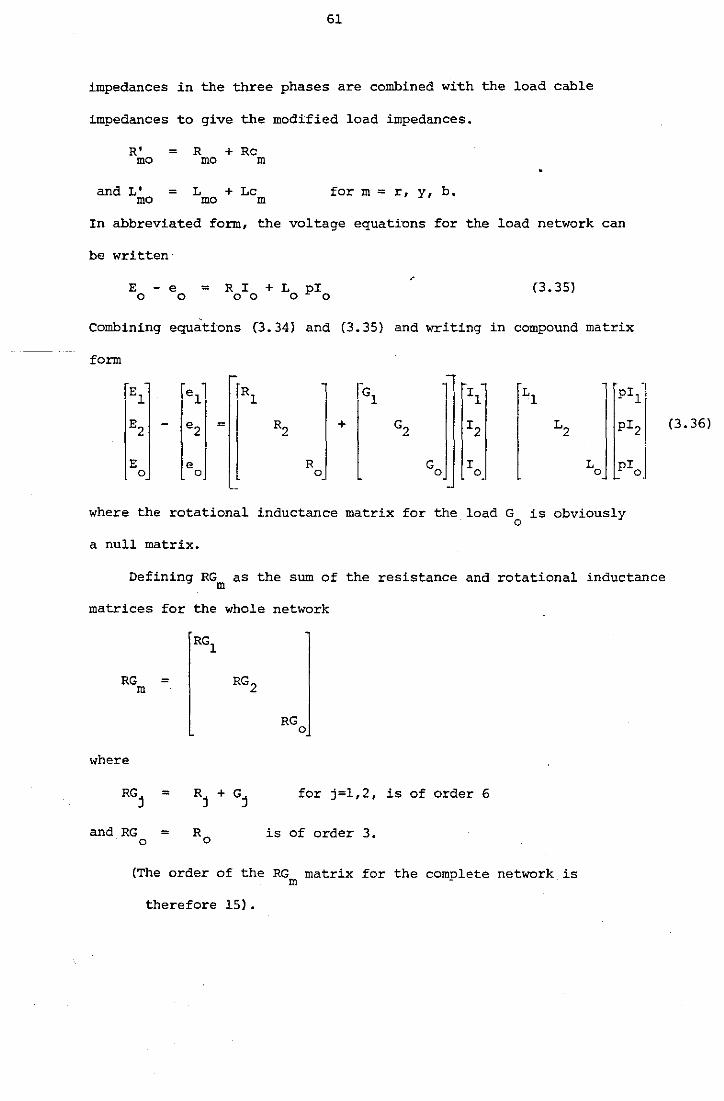
Combining equations (3. 34) and (3.35) and writing in compound matrix
form
rEl e 1l [Rl
•[G' ll ri Ll pil 1
E2 e2 = R2 G2 I2 L2 pi2
E e R Go I L pioj 0 0 0 0 0
where the rotational inductance matrix for the load G is obviously 0
a null matrix.
Defining RG as the sum of the resistance and rotational inductance m
matrices for the whole network
RG = m
where
and RG 0
=
=
RG 0
for j=l,2, is of order 6
is of order 3.
(The order of the RG matrix for the complete network is m
therefore 15).
(3.36)
62
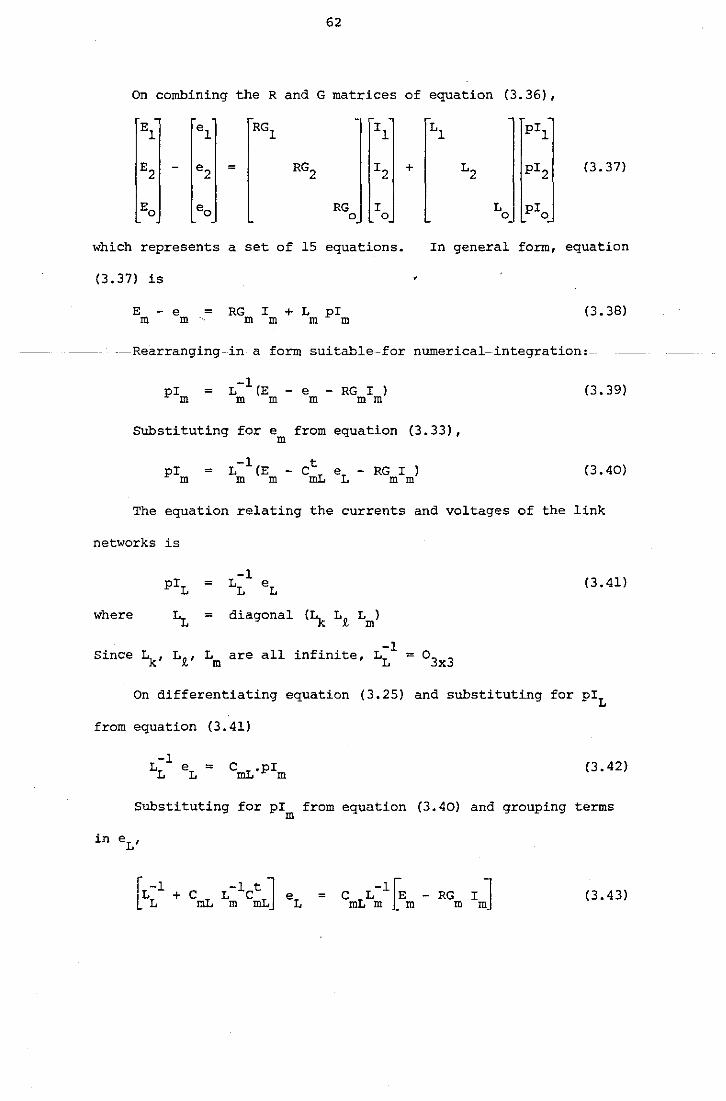
On combining the R and G matrices of equation (3.36).
El el RG1 Il Ll pil
E2 e2 = RG2 I2 + L2 pi2 (3.37)
Eo eo RG I L pia 0 0 0
which represents a set of 15 equations. In general form, equation
(3.37) is '
E - e = RG I + L pi (3.38) m m m m m m
---Rearranging in a form suitable-for numerical-integration:-
pi = m
L -l (E - e - RG I ) m m m m m
Substituting fore from equation (3.33), m
pi = m
-1 t L (E - C eL - RG I ) m m mL mm
(3. 39)
(3. 40)
The equation relating the currents and voltages of the link
networks is
= (3.41)
where =
Since ~· Li, Lm are all infinite, L~l = o3x3
On differentiating equation (3.25) and substituting for piL
from equation (3.41)
(3. 42)
Substituting for pi from equation (3.40) and grouping terms m
= -lG C L E -mL m m
RG m
(3.43)
63
L -l + CmLL~t then, L mmL
If Y = since = 0 as before,
equation (3.43) can be simplified to
=
and on substituting for eL in equation (3.40)
pi m
=
where U is a unit matrix of order 15.
[E - RG I ] m mm
Equation (3.45) can also be written as
pim = -L:iu- c~[cmLL:lc~r\mLL:l}[Em_- RG m
which may be solved for I on a step-by-step basis, using the m
numerical integration technique discussed in Appendix 2.
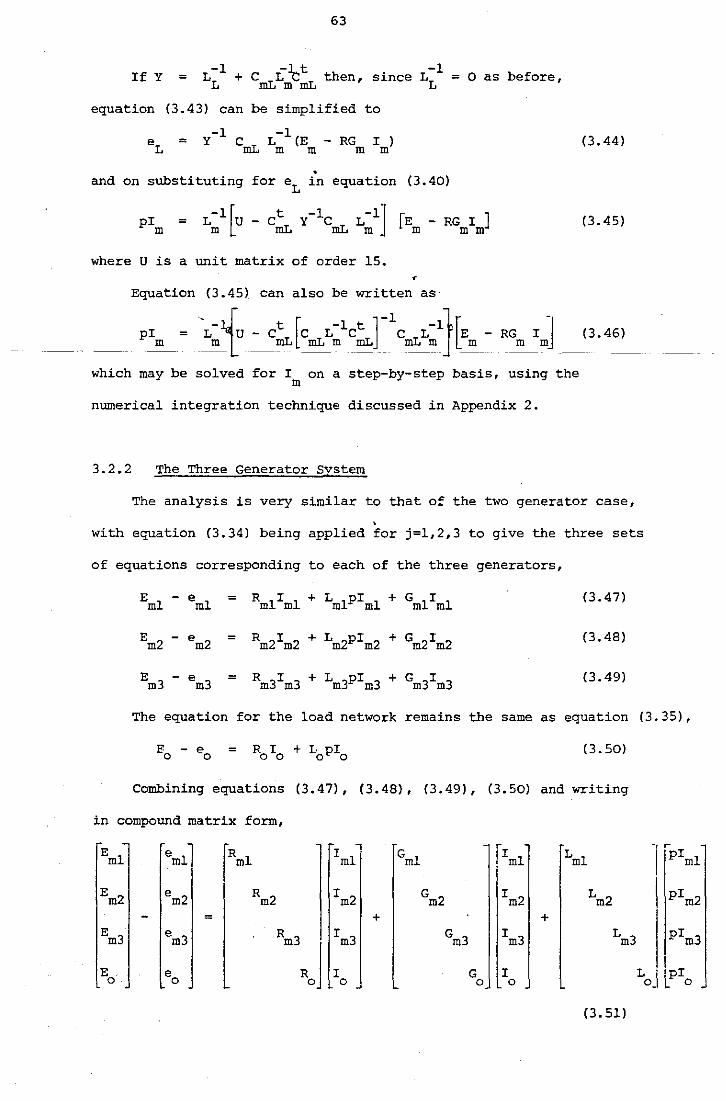
3.2.2 The Three Generator System
( 3. 44)
(3.45)
(3.46)
The analysis is very similar to that of the two generator case, .
with equation (3.34) being applied for j=l,2,3 to give the three sets
of equations corresponding to each of the three generators,
= (3.47)
= (3.48)
= (3. 49)
The equation for the load network remains the same as equation (3.35),
E - e 0 0
= ( 3. 50)
Combining equations (3.47), (3.48), (3.49), (3.50) and writing
in compound matrix form,
Eml eml Rml Iml Gml Iml Lml -~ ,-piml
Em2 em2 Rm2 Im2 Gm2 Im2 Lm2 pim2
= + + Em3 em3 Rm3
RJ
Im3 Gm3 Im3 Lm3 pim3
E e I G I L pi 0 0 0 0 0 0 0 -
(3. 51)
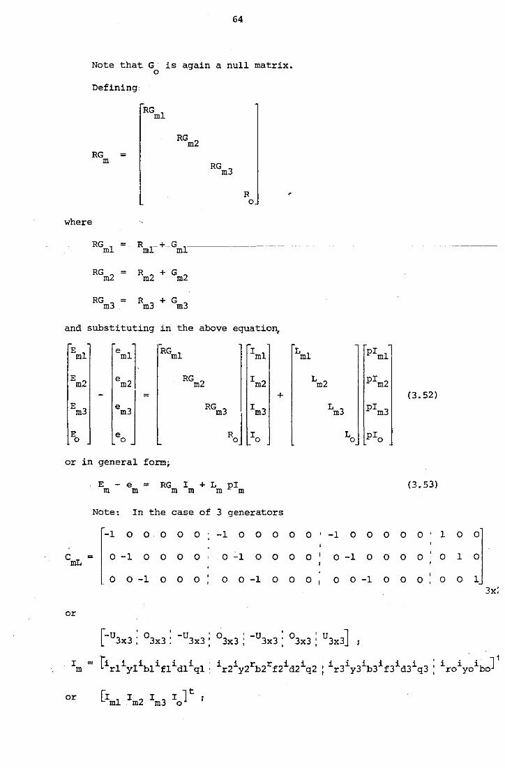
64
Note that G is again a null matrix. 0
Defining'
RG = m
R 0
where
RGml = Rml-+ Gml
RGm2 = Rm2 + Gm2
RG = m3 Rm3 + Gm3
and substituting in the above equation,
-Eml RGml Iml Lml piml
Em2
·.,l em2 RGm2 Im2 Lm2 pim2
::'J = + (3.52)
Em3 RGm3
R0j
Im3 Lm3 pim3
E Io Lo pie 0
or in general form;
E - e = RG I + L pi m m m m m m (3. 53)
Note: In the case of 3 generators
r-: 0 0 0 0 0 -1 0 0 0 0 0 ' -1 0 0 0 0 0
cmL = -1 0 0 0 0 0 -1 0 0 0 0 0 -1 0 0 0 0
[o 0 -1 0 0 0 0 0 -1 0 0 o, 0 0 -1 0 0 0
or
r . . -u3x3; 0 3x3: -u3x3; 0
3x3; -U3x3 : 03x3 : u3x3] 1
I = [irl1yiibl1fl1dliql: 1r2iy2rb2rf21d2 1q2 I i 3i 3ib3if3id31 3 ; m ' r y q '
or [I l I 2 I 3
I lt m m m o
1 0
:j 0 1
0 0 3x:
i i. i ] 1 ro yo bo
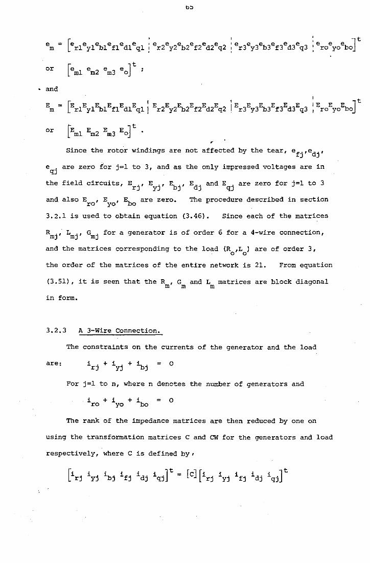
• - t 'e e e J : royobo
and I t I E E E J 1 ro yo bo
Since the rotor windings are not affected by the tear, efj'edj'
eqj are zero for j;l to 3, and as the only impressed voltages are in
the field circuits, Erj' Eyj' Ebj' Edj and Eqj are zero for j;l to 3
and also Ere' Eye' Ebo are zero. The procedure described in section
3.2.1 is used to obtain equation (3.46). Since each of the matrices
Rmj; Lmj' Gmj for a generator is of order 6 for a 4-wire connection,
and the matrices corresponding to the load (R ,L J are of order 3, . 0 0
the order of the matrices of the entire network is 21. From equation
(3.51), it is seen that the R , G and L matrices are block diagonal m m m
in form.
3.2.3 A 3-Wire Connection.
The constraints on the currents of the generator and the load
are: ; 0
For j;l to n, where n denotes the number of generators and
; 0
The rank of the impedance matrices are then reduced by one on
using the transformation matrices c and CW for the generators and load
respectively, where C is defined by•
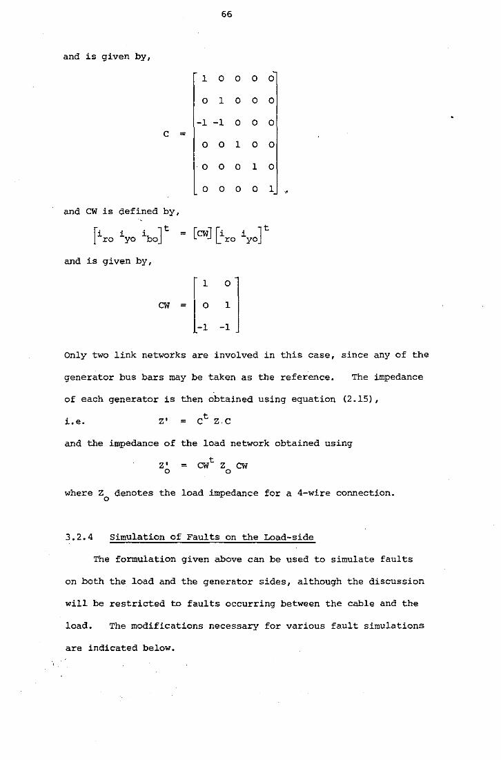
66
and is given by,
1 0 0 0 0
0 1 0 0 0
-1 -1 0 0 0 c =
0 0 1 0 0
0 0 0 1 0
0 0 0 0 1 '
and cw is defined by,
[iro i i t = [cw] [i i t yo bo ro yo
and is given by,
I 1
J cw = l-: Only two link networks are involved in this case, since any of the
generator bus bars may be taken as the reference. The impedance
of each generator is then obtained using equation (2.15),
i.e. Z' = et z.c
and the impedance of the load network obtained using
Z' 0 = cwt z
0 cw
where Z denotes the load impedance for a 4-wire connection. 0
3.2.4 Simulation of Faults on the Load-side
The formulation given above can be used to simulate faults
on both the load and the generator sides, although the discussion
will be restricted to faults occurring between the cable and the
load. The modifications necessary for various fault simulations
are indicated below.
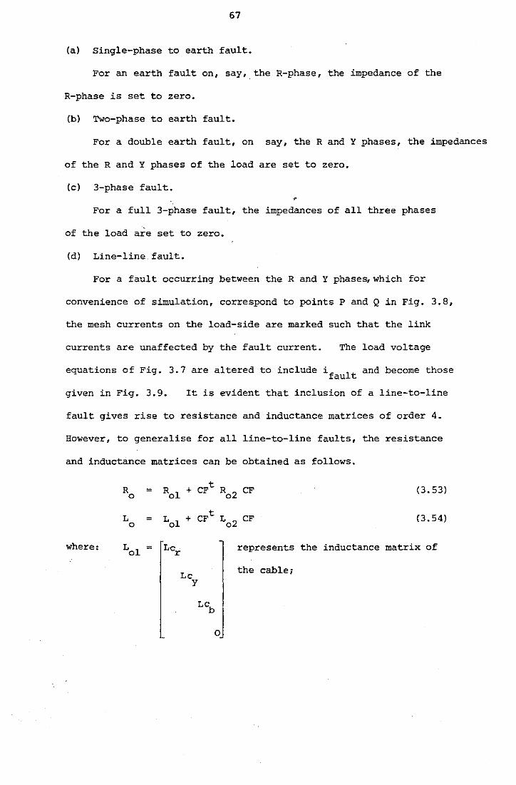
67
(a) Single-phase to earth fault.
For an earth fault on, say, the R-phase, the impedance of the
R-phase is set to zero.
(b) Two-phase to earth fault.
For a double earth fault, on say, the R and Y phases, the impedances
of the R and Y phases of the load are set to zero.
(c) 3-phase fault. •
For a full 3-phase fault, the impedances of all three phases
of the load a~e set to zero.
(d) Line-line fault.
For a fault occurring between the Rand Y phase~which for
convenience of simulation, correspond to points P and Q in Fig. 3.8,
the mesh currents on the load-side are marked such that the link
currents are unaffected by the fault current. The load voltage
equations of Fig. 3.7 are altered to include ifault and become those
given in Fig. 3.9. It is evident that inclusion of a line-to-line
fault gives rise to resistance and inductance matrices of order 4.
However, to generalise for all line-to-line faults, the resistance
and inductance matrices can be obtained as follows.
Ro = Rol + CFt Ro2 CF
L0
= L01
+ CFt L02
CF
(3.53)
(3.54)
where: represents the inductance matrix of
Le y
L~
0
the cable;
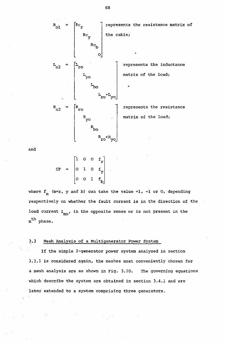
=
=
=
and
CF =
68
Re r
represents the resistance matrix of
Re the cable; y
L yo
R yo
R~
0
L +L ro yo
R +R ro yo
1 0 0 f r
0 1 0 f y
0 0 1 fb
represents the inductance
matrix of the load;
represents the resistance
matrix of the load;
where f (m=r, y and b) can take the value +1, -1 or o, depending m
respectively on whether the fault current is in the direction of the
load current i , in the opposite sense or is not present in the mo
th m phase.
3.3 Mesh Analysis of a Multigenerator Power System
If the simple 2-generator power system analysed in section
3.3.1 is considered again, the meshes most conveniently chosen for
a mesh analysis are as shown in Fig. 3.10. The governing equations
which describe the system are obtained in section 3.4.1 and are
later extended to a system comprising three generators.
69
3.3.1 The Two-Generator System.
In the case of a 4-wire connection, there are three meshes
associated with the generator armature and the load for each machine,
in addition to the three meshes for the rotor circuits of each machine.
Note: As in section 3.2.1, the resistance and inductance of each
phase of the transmission line are included with the corresponding
• armature winding terms to give modified armature resistances
and inductances respectively;
R' = R + Rt m m m
L' = L + Lt for m = r, y and b, mm mm m
holds for both generators.
Similarly, the resistance and inductance of the cable are combined
with the corresponding load resistance and inductance respectively to
give modified load resistances and inductances of
R' mo =
L' = L + Le mo mo m for m = r, y and b.
In establishing the system equations, the mesh currents will
be indicated by i ., where j = 1,2 identifies the individual generators mJ
and m can take the suffixes r, y, b, f, d, or q, depending on
whether it is associated with the r-phase, y-phase, b-phase armature
windings, or the field, d-axis and q-axis damper winding.
Applying Kirchhoff's voltage law to mesh G1R1RLN of Fig.
3.10, it follows that
= 0 (3. 55)
70
(R'+R' )i 1+R' i 2+p(L' +L' )i 1+pM i 1 +pM bibl+pM fifl + yyoy yoy yyyoy ryr y y
= 0 (3. 56)
= 0 (3. 57)
Similarly, for the rotor circuits,
= (3. 58)
= 0 (3.59)
R i 1+pM i 1+pM i 1+p~ ibl+pL i l qq rqr yqy nq qqq = 0 (3.60)
Equations (3.55) to (3.60), re-written in matrix form are given
in Fig. 3.11 in which,
L'' = L' + L' m nnn mo
and R1 I = R' + R'
m m mo for m = r, y and b.
For generator 2, applying Kirchhoff's voltage law to mesh G2
R2
RLN,
(R'+R' )i 2+R' i l+p(L' +L' )i 2+pM i 2+pM bib2+pM fif2
+ rror ror rrror ryy r r
+pM did2+pM i 2+L' pi l = 0 r rqq ror (3. 61)
Similarly, for mesh G2
Y2
YLN,
(R'+R' )i 2+R' i 1
+p(L' +L' )i 2+pM i 2
+pM bib2
+pM fif2
+ yyoy yoy yyyoy ryr y y
= 0 (3.62)
.'F},+Rbc,lib2+Rbc,ibl+pCLt,b+Lix,lib2+p~yib2+p~rir2+p~fif2 +
+p~d1d2+p'\,qiq2+Lix,pibl = 0 (3. 63)
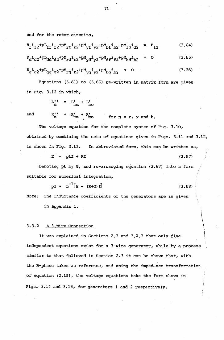
71
and for the rotor circuits,
= (3.64)
= 0 (3.65)
= 0 (3. 66)
Equations (3.61) to (3.66) re-written in matrix form are given
in Fig. 3.12 in which,
L' I = . L 1 + L' m mm mo
and R 1 I = R' + R'
m mm mo for m = r, y and b.
The voltage equation for the complete system of Fig. 3.10,
obtained by combining the sets of equations given in Figs. 3.11 and 3.12,
is shown in Fig. 3.13. In abbreviated form, this can be written as,
E'= pLI+RI (3.67)
Denoting pL by G, and re-arranging equation (3.67) into a form
suitable for numerical integration,
(3. 68)
Note: The inductance coefficients of the generators are as given
in Appendix. 1.
3.3.2 ~ 3 Wire Connection
It was explained in Sections 2.3 and 3.2.3 that only five
independent equations exist for a 3-wire generator, while by a process
similar to that followed in Section 2.3 it can be shown that, with
the B-phase taken as reference, and using the impedance transformation
of equation (2.15), the voltage equations take the form shown in
Figs.· 3.14 and 3.15, for generators 1 and 2 respectively.

72
3.3.3 The 3-Generator System
By applying mesh analysis to each of the meshes associated
with each generator, it can be shown that for a 4-wire connection
the voltage equations have the form given in Fig. 3.16. In general,
it can be seen that the impedances of the network of a 2-generator
or 3-generator system are isomorphic. The total number of independent
equations of a 3-generator system, for a'4-wire connection, is 18
and that for a- 3-wire connection is 15. Thus it follows that for
an n-generator system, the number of independent equations can either
be 6n or Sn, depending on whether it is a 3-wire or 4-wire connection.
3.3.4 Simulation of Faults on the Load-side
In the same manner as when the diakoptic approach was investigated,
the simulation of faults will be considered for the load-side only.
The modifications necessary for various conditions are indicated
below.
(a) Single-phase to earth fault.
The impedance of the load in the faulted phase is set to zero,
i.e. if the fault occurs on the R-phase of the load, R and L ro ro
both become zero.
(b) Two-phase to earth fault.
The impedances of the load in the faulted phases are set to zero.
(c) 3-phase to earth fault.
In this case, the impedances of all phases of the load are set
to zero, so that R = 0 and L = o for m = _r, y and b. mo mo
(d) Line-to-line fault.
Here, an additional mesh current appears, due to the fault current
circulating between the short circuited lines. For the example shown
73
in Fig. 3.17 with a line-to-line fault between the R and Y phases
of the load of a 2-generator system, a mesh analysis yields the set
of voltages equations given in Fig. 3.18.
3.4 Disadvantages of the Mesh Analysis Approach.
Unlike the diakoptic approach, the application of mesh analysis .. to larger networks ·is a very laborious process, which is not practicable
with large-scale networks. Since the resistance and inductance
matrices consist of non-zero off-diagonal elements, complete matrices
have to be stored for computational purposes. In addition, matrix
inversion also becomes a very lengthy process, with the time involved
in the matrix inversion being approximately proportional to the cube
of the matrix order. However, in the diakoptic approach, since the
resistance and inductance matrices involved are all of block diagonal
form, for computational purposes- only the individual blocks on the
leading diagonal need to be stored. This represents a considerable
saving in computer run-time, as the inversion process requires the
inversion of individual matrices with the largest being of order 6.
In the situation of identical generators, the storage of a single matrix
only is necessary in the diakoptic approach.
3.5 Digital Simulation
From the analyses of sections 3.2 and 3.3~ it can be seen that
the equations which govern the type of system under investigation can '·
be expressed in the general form,
(3. 69)
where L, R, G are inductance, resistance and rotational inductance
matrices respectively, E is the impressed voltage vector, I the current
·.•·
74
vector and ~ is a factor which depends on the way the equations are
formulated • ~ is a unit matrix U for mesh analysis and is •
for a diakoptic analysis. Using the formulation of equation (3.69)
numerical integration is carried out using the technique described in
Appendix 2 on a step-by-step basis, to evaluate the current vector.
Programs were developed in Fortran IV and run on an ICL 1904 machine,
with the solution processes for both formulations being discussed in
the following sections.
3.5.1 Simulation .. Using the Diakoptics Formulation
Fig. 3.19 shows a simplified flow chart of the computer program
used for the diakoptic formulation. The steps leading to the
solution are as follows:
(l) Read in initial data: number of generators, type of connection,
frequency, number of independent studies, step length of integration,
resistances and inductances of the generator windings, transmission
lines, cables and load; time duration of each study.
(2! · Set up the resistance matrix for each generator and the load.
(3)
(4)
If it is a 3-wire connection, use the transformation matrices C
and CW of Section 3.2.3; the resistance of each generator is
then obtained using equation (2.15!, and the resistance of the
load using the transformation CWtR CW (See Section 3. 2. 3). 0
t Set up the mesh/link _transformation matrices CmL and CmL.
Form the inductance matrix L and the rotational inductance
matrix G. Determine the factor ~.
(5) Integrate numerically equation (3.69), and evaluate the mesh
current vector.
75
(6) Determine the link voltage vector using equation (3.44) and
hence the voltages at the terminals of the generators and load.
(7) Advance the calculations by one step. Proceed to instruction
(4) until the end of the study is reached. A new study is then
commenced by proceeding to instruction (2) and the process
repeated until all the studies are completed.
3.5.2 Simulation Using the Mesh Analysis Formulation
A simplified flow chart for the computer program is given
in Fig. 3.20. The procedure leading to the solution of the mesh
currents I of equation (3.69) is described briefly as follows.
(1) Set up the initial conditions of the network, i.e. the number
of generators, inductance and resistance parameters of the network,
frequency, initial mesh currents of the network, the number and
type of independent studies to be considered and the time
duration of the entire simulation.
(2) Form the resistance matrix at the start of the simulation.
This matrix remains unchanged, unless a line-to-line fault is
simulated, in which case the order of the matrix increases by
one (see section 3.3.4} • .. (3) Form the impressed voltage vector E.
(4) Form the inductance and rotational inductance matrices L and G,
respectively.
(5) Since for a mesh analysis ~.is a unit matrix, the product
-1 -1 L ~ becomes L • Evaluate pi using equation (3.69), and using
the integration technique described in Appendix 2, the solution
for I is obtained.
(6) The voltages across each phase of the load is then obtained
using the relationship
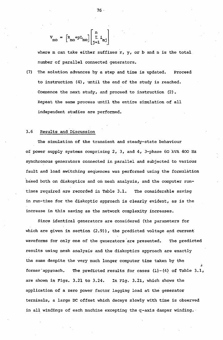
V mo
76.
= [R +pL J[~ijJ mo mo j;.,l m
where m can take either suffixes r, y, or b and n is the total
number of parallel connected generators.
(7) The solution advances by a step and time is updated. Proceed
to instruction (4), until the end of the study is reached.
Commence the next study, and proceed to instruction (2).
Repeat the same process until the entire simulation of all
independent studies are performed.
3.6 Results and Discussion
The simulation of the transient and steady-state behaviour
of power supply systems comprising 2, 3, and 4, 3-phase 60 kVA 400 Hz
synchronous generators connected in parallel and subjected to various
fault and load switching sequences was performed using the formulation
based both on diakoptics and on mesh analysis, and the computer run-
times required are recorded in Table 3.1. The considerable saving
in run-time for the diakoptic approach is clearly evident, as is the
increase in this saving as the network complexity increases.
Since identical generators are considered (the parameters for
which are given in section (2.9)), the predicted voltage and current
waveforms for only one of the generators are presented. The predicted
results using mesh analysis and the diakoptics approach are exactly
the same despite the very much longer computer time taken by the
former·approach. The predicted results for cases (1)-(4) of Table 3.1,
are shown in Figs. 3.21 to 3.24. In Fig. 3.21, which shows the
application of a zero power factor lagging load at the generator
terminals, a large DC offset which decays slowly with time is observed
in all windings of each machine excepting the q-axis damper winding. ·
77 J
This is because at zero power factor lagging, the armature reaction
is centred along the d-axis and therefore there is no component in the
direction of the q-axis.
Fig. 3.22 shows the sudden application of a 2-phase to earth
fault (R and Y phases being faulted) on a 2-generator system, running on
steady-state rated load at 0.8 power factor. During the steady-state
load condition, a very rapid decay of the DC component is observed and,
as a result, no oscillatory components are seen in the rotor circuits
(see Figs. 3.22(a), (bl and (c)). However, on the application of
a 2-phase to earth fault, due to the unbalanced mmf situation existing
in the armature windings, higher harmonic currents are induced in the
rotor circuits. The fundamental and second harmonic currents only
are clearly seen. The circulating fault current between phases
Rand Y is seen to rise to 2850A and is shown in Fig. 3.22(g). Due
to the fault condition a rise in currents in the R and Y phases are
observed, while the B-phase current drops. The short circuit across
the R and Y phases is seen .to cause a large drop in the terminal
voltages of the Rand Y phases (see Figs. 3.22(hJ and (i)).
The sequential application of 0.8 power factor rated load, line-to
line fault on R and Y phases and 3-phase short circuit is shown in
Fig. 3.23. As mentioned before, the application of 0.8 power factor
rated load does not cause oscillatory currents to be induced in the
rotor windings due to the rapid decay of the DC component. Since
this simulation is for a 3-generator system, the fault currents are
much higher and the circulating fault current between phases R and Y
is of the order of 3700 Amps. Just prior to the application of the
3-phase short circuit, the currents are somewhat steady and therefore
on the application of the full short circuit, the currents do not
rise as much as these would do if a fault was absent prior to the full
..
78
short circuit. About 0.25 secs after the application of the 3-phase
short circuit, the DC component has decayed and therefore no currents
are observed in the d,q damper windings (see Figs. 3.23(b) and (c)).
The case of the application of rated load at 0.8 power factor to
B-phase to earth fault to Y-B phase to earth to rejection of load is
considered in Fig. 3.24. Due to the unbalanced mmf in the armature
during the single-phase to earth and double-phase to earth faults,
higher harmonic currents are induced in the rotor windings and are
seen in Figs. 3.24(a), (b) and (c). The R-phase load current is
seen to decrease as the number of phases faulted (B & Y) increases
(see Fig. 3.24(g)).. On rejection of load the voltage build up is
initially rapid and then more gradual as seen in the terminal voltages
of the Rand Y phases (see Figs. 3.24(h) and (i)}.
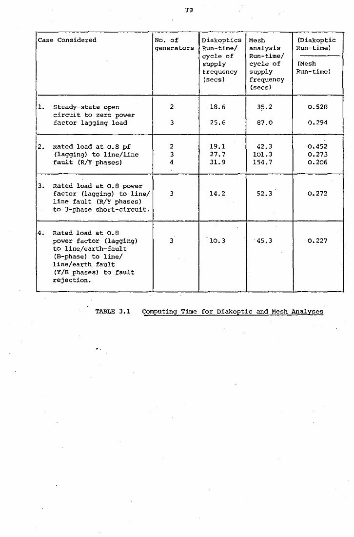
79
Case Considered No. of Diakoptics Mesh (Diakoptic generators ! Run-time/ analysis Run-time)
, cycle of Run-time/ supply cycle of (Mesh frequency supply Run-time) (secs) frequency
(secs) '
11. Steady-state open 2 18.6 35.2 0.528 circuit to zero power
I factor lagging load 3 25.6 87.0 0.294
I 2. Rated load at 0,8 pf 2 19.1 42.3 0.452
(lagging) to line/line 3 27.7 101.3 0.273 fault (R/Y phases) 4 31.9 154.7 0.206
.
3. Rated load at 0.8 power factor (lagging) to line/ 3 14.2 52.3 0.272 line fault (R/Y phases) to 3-phase short-circuit.
4. Rated load at 0.8 power factor (lagging) 3 10.3 45.3 0.227 to line/earth-fault (B-phase) to line/ line/earth fault (Y/B phases) to fault rejection.
.
TABLE 3.1 ~omputing Time for Diakoptic and Mesh Analyses
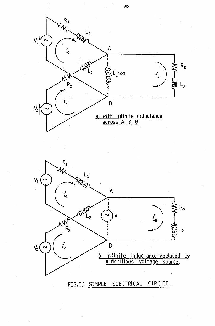
80
A
B
a. with infinite inductance across A & 8
A
I I , .....
f-v\e \ I L
.. T, I I
B
b. infinite inductance replaced by a f1chhous voltage source.
FIG. 3.1 SIMPLE ELECTRICAL CIRCUIT.
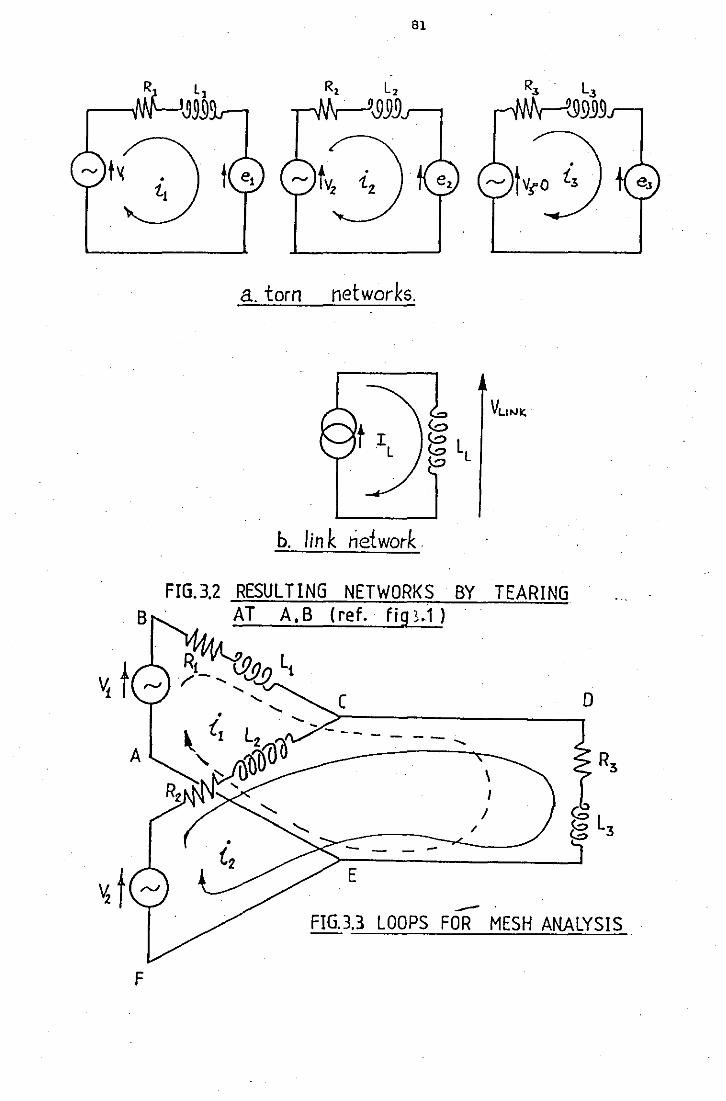
81
a. torn networks.
b. I ink network.
FIG.3.2 RESULTING NETWORKS BY TEARING AT A,B (ref.· fig~.1 l
( 0
------ .....
/
- --E
---· FIG.3.3 LOOPS FOR MESH ANALYSIS
F
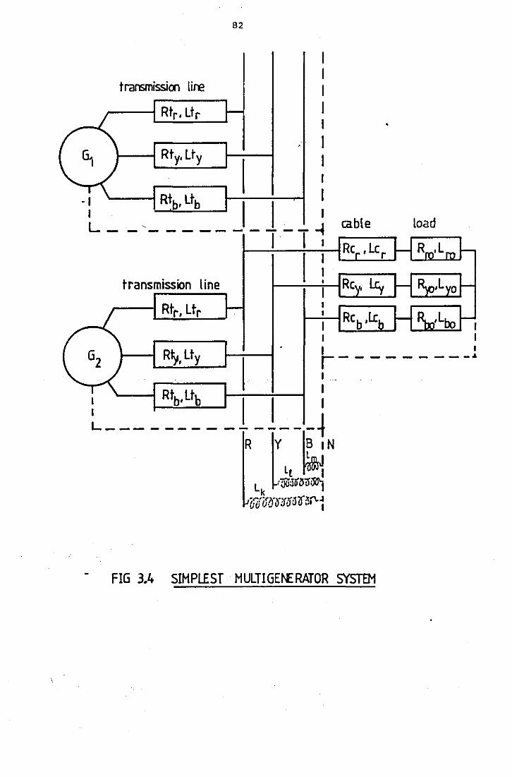
I
transmissioo lire
./ ~ Rtr, Ltr
~ Rty. Lty
T\ I - I 1 Rtb, Ltb I
82
1-
I I
.
I
I I I I
L - - ,_ - - -- - - - -- -1 I ·. I I
cable
transmission line I ! 1-::_
1 -1 Rcb ,Le
I
load
t---f R~, Lty I I r-------- _ .. I I
: Rtb, Ltb I I I
L---- ------ -----i R L.~N
Lk --I
ocro:~·o·oo~ifal'-~
FIG 3.4 SIMPLEST HULTIGE~RATOR SYSTEM
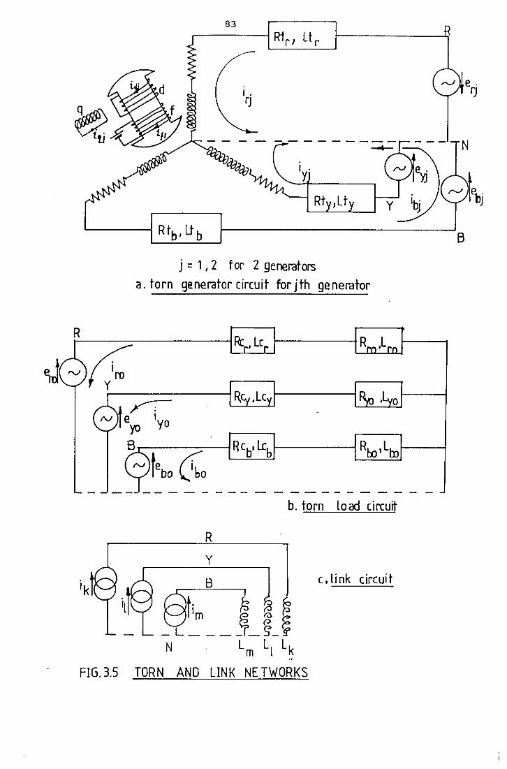
83
B
j = 1 , 2 tor 2 generators a. torn generator circuit for jth generator
R
~ eyo 'yo
B ..-------:-----4 R cb' l.cb 1----~ Roo' Lbo 1-----l
rv febo 0o b. torn load circuit
R
y
B c.link circuit
~~;m ---~-t! N Lm Ll Lk
FIG. 3.5 TORN AND LINK NETWORKS
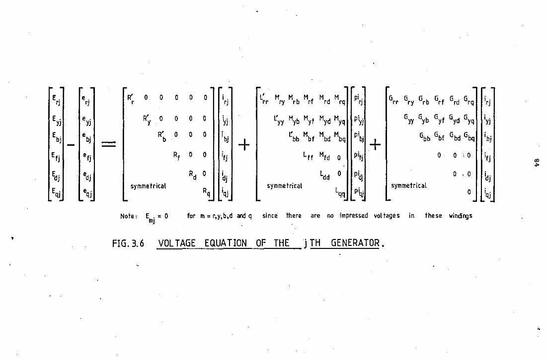
Erd I e rj I I R~ 0 0 0 0 0 11 ird IL' M M M M M 11 ° I rr ry rb rf rd rq p1rj I Grr Gry Grb Grf Grd Grq i 0
rJ
Eyj e 0 R' 0 0 0 0 ~j i:yy Myb Myf Myd Myq P~j Gyy Gyb Gyf Gyd Gyq i 0
YJ y YJ
Ebj ebj R' 0 0 0 i bj ~bb Mbf Mbd Mbq pibj Gbh Gbf Gbd Gbq ibj - b + + Efjj I efj I I Rf 0 o I Ptj Lff Mfd 0 pifj 0 0 '0 ifj I "' .j>o
Edj edj Rd 0 ~j Ldd 0 p~j 0 °, 0 idj
Eqj e 0
symmetrical Rq iqj
symmetrical Lqq p~
symmetrical i 0 QJ 0 QJ
0
Note: E 0 = 0 for m= r,y,b,d and q since there are no impressed voltage s in the se windings mJ
• FIG.3.6 VOLTAGE EQUATION OF THE j TH GENERATOR.
~
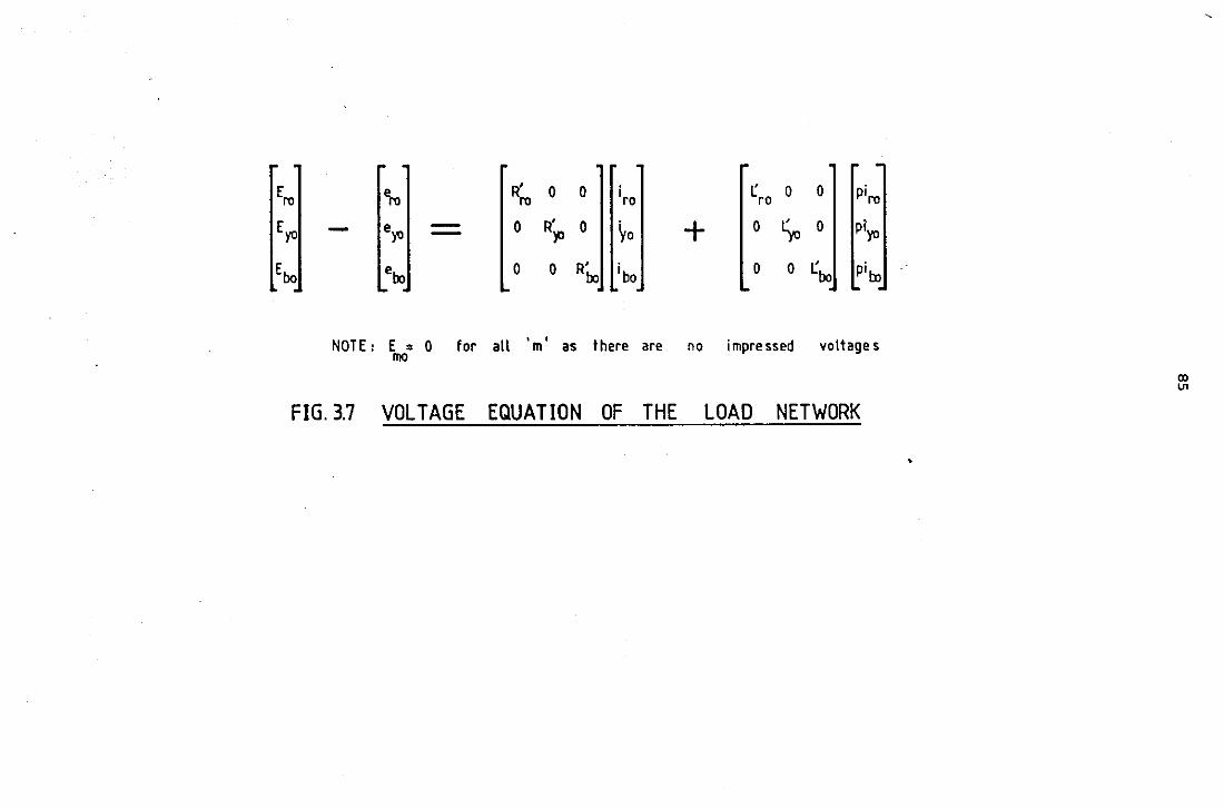
R' ro 0 0
- 0 R' 'fJ
0
0 0 R' 00
ire
~0 + ibo
t: o o . ro P'ro
0 ~ 0
0 o t: 00
NOTE: E = 0 for all 'm' as there are no impressed voltage s mo
FIG. 3.7 VOLTAGE EQUATION OF THE LOAD NETWORK
'
(X) U1
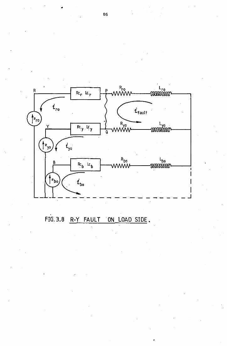
R
86
ifaul t
Rcy. U:y
Lbo Rcb . L!:b r-....... ~~,,...AA,MJ.---...t;\]umao~lll'-----l1
FIG. 3.8 R-Y FAULT ON LOAD SIDE.
I I I
_ _J
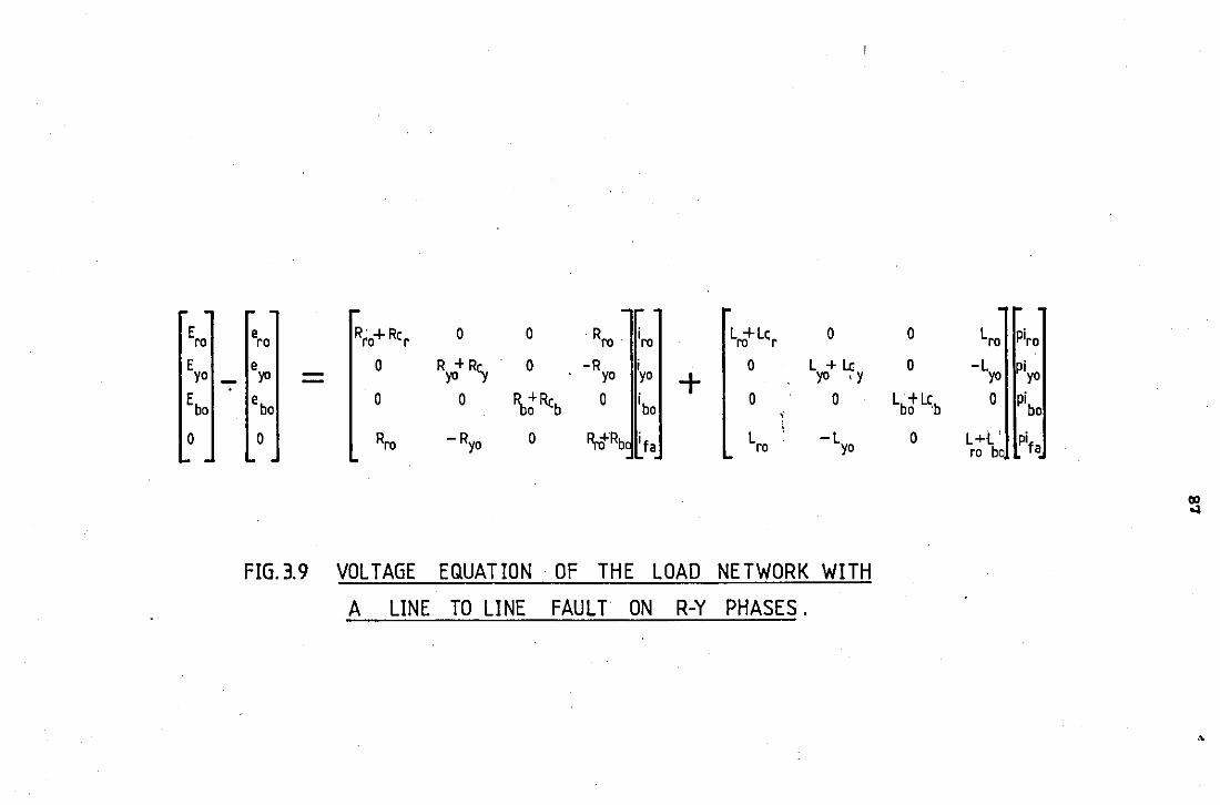
E e Rro+ Rcr 0 0 R iro L +Le 0 0 Lro Piro ro ro ro· ro r E e 0 Ryo+ R)o 0 -R 0 L+Lc 0 -L piyo yo - yo yo yo + yo 'y yo
Ebo ebo 0 0 fbci"Rcb 0 ibo 0 0 Lbci Ll;b 0 pibo '
~llb if a Lro \
-L 0 L+l' pi fa 0 0 Rro -Ryo 0 yo ro bo
CIO ~
FIG. 3.9 VOLTAGE EQUATION OF THE LOAD NETWORK WITH
A LINE TO LINE FAULT ON R-Y PHASES.
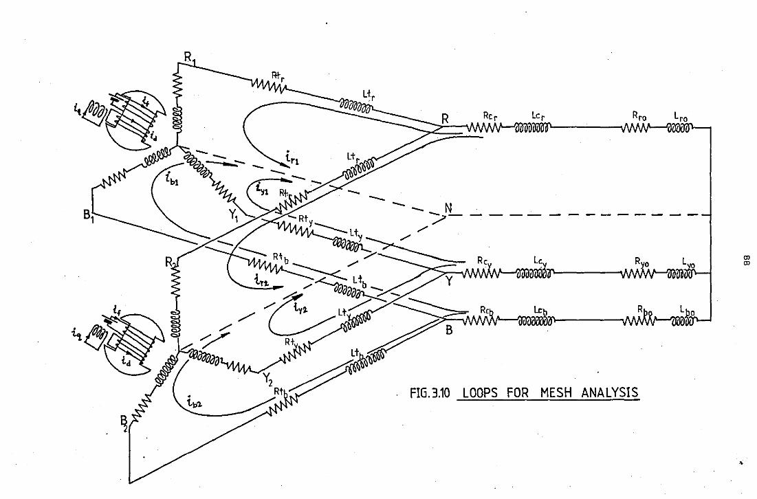
R
-.._N_-?
---;::><;:.;-:;-V~wvv. • uoil~lil"--- '" ·
FOR MESH ANALYSIS
·•
"' "'
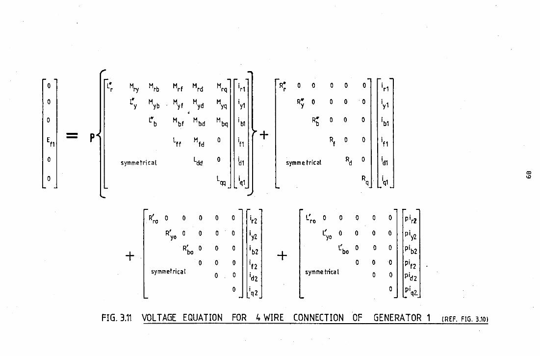
0 L• r Mry Mrb Mrf Mrd Mrq ir1 R•
r 0 0 0 0 0 ir1
0 !.* Myb Myf Myd Myq iy1 R., 0 0 0 0 iy1 y y
0 ~ b Mbf Mbd Mbq i b1 R' b 0 0 0 ib1
- p + Ef1 - Lff Mfd 0 if1 Rf 0 0 if 1
0 symmetrical Ldd 0 id1 symmetrical Rd 0 id1
a> 0 Lqq iq1 Rq iq1
ID
R' ro 0 0 0 0 0 irz L'ro 0 0 0 0 0 pir2
R' yo 0 0 0 0 iy2 ~yo 0 0 0 0 piy2
R' 0 0 0 ib2 ( 0 0 0 pib2 + bo + bo
0 0 0 if2 0 0 0 pif2 symmetrical
0 0 idZ symme trica 1 0 0 pidZ
0 iq2 0 piq2.
FIG. 3.11 VOLTAGE EQUATION FOR 4 WIRE CONNECTION OF GENERATOR 1 (REF. FIG. 3.101
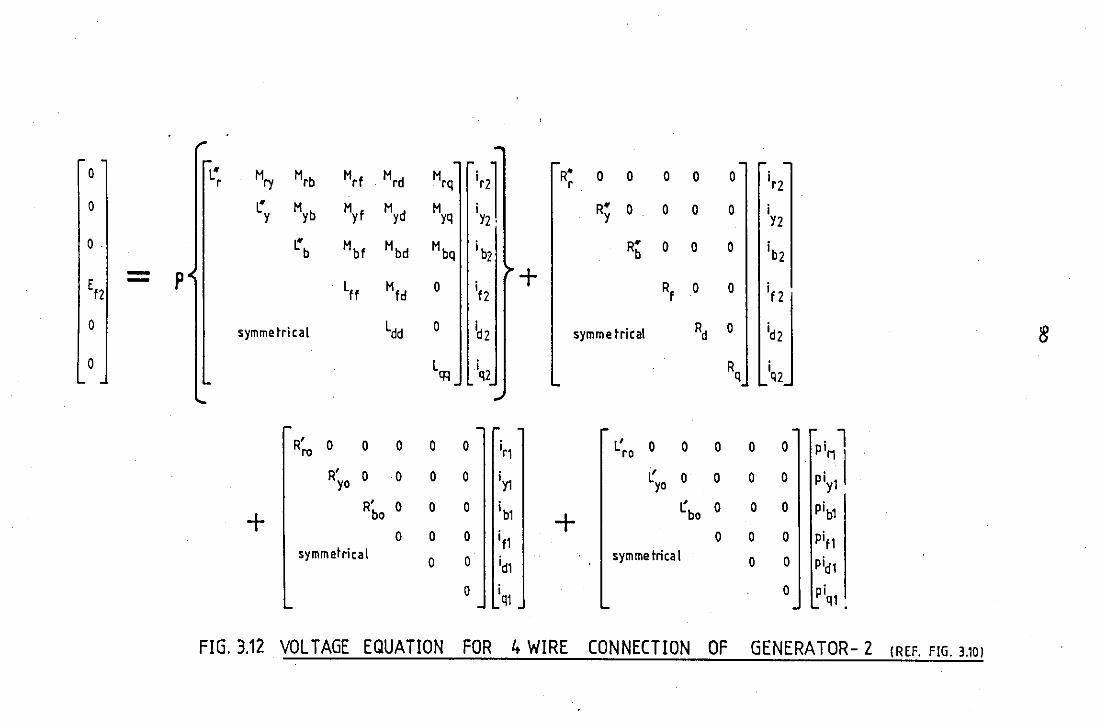
0 L" Hry Hrb Hrf Hrd Hrq :r21
R• 0 0 0 0 0 ir2 r r
0 1.' Hyb Myf Hyd Myq R" 0 0 0 0 i y Y2 · y Y2
0 . L' b Mbf Hbd Hbq i b2 R' b 0 0 0 ib2 - p + Ef2 - Lff Mid 0 if2 Rf 0 0 if 2
0 symmetrical Ldd 0 b symmetrical Rd 0 id2
0 LQ:l iq2 Rq iQ2
R' 0 0 0 0 0 ir1 L'ro 0 0 0 0 0 ' 1 ro p:~ I
R'yo 0 0 0 0 iY1 L'yo 0 0 0 0 Plyl
R' 0 0 0 ib1 L' 0 0 0 pib1 + bo + bo
0 0 0 i t1 0 0 0 pif1 symmetrical
0 0 id1 symmetrical 0 0 pid1
0 iq1 0 piq1
FIG. 3.12 VOLTAGE EQUATION FOR 4 WIRE CONNECTION OF GENERATOR- 2 (REF. FIG. 3.10!
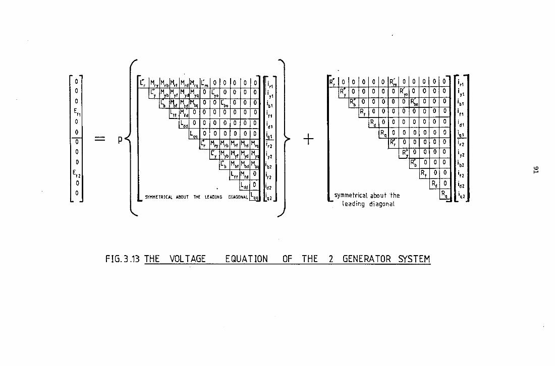
0 0
0
E., 0
0 0
0
0
E,2 0 0
/
L' '
M,, M,b M,, M,, M,, r .. 0 t.:' Myb M,, M M 0 t.:
y y " yo
c. M,, Mbd M, 0 0
Ltt Mid 0 0 0
L,, 0 0 0
p L:.. 0 0 c, M.,
(' y
.
0 0 0 0 0 0
r bo 0 0
0 0 0
0 0 0
0 0 0
M,b M.t M,
~ Myt M,. r b Mbt ~d
Ltt Mfd
L,,
0 0
0 0
0
0
M,.
M,
M, 0
0
ff""
,i
'· ,, ,, y1
b1 i
i
i
i
f1
d1
.:1!.. i, 2
i y2
2 ib
i,
;, 2
2
I. SYHHETRICAL ABOUT THE L£A01NG DIAGONAL~ ~.
FIG. 3 .13 THE VOLT AGE EQUATION
if. 0 0 0 0 0 R' .. 0 0 0
R 0 0 0 0 0 R,. 0 0 y
Rb 0 0 0 0 0 R;,. 0
R, 0 0 0 0 0 0
R, 0 0 0 0 0
+ R, 0 0 0 0
R; 0 0 0
R• 0 0
IR'b 0
R,
symmetrical about the '- . .
tead1ng d1agonat
OF THE 2 GENERATOR SYSTEM
0 0-
0 0
0 0
0 0
0 0
0 0 0 0
0 0
0 0
0 0
R, 0
~
... i i
i
i
i
i i
i
i
i
i
,, y1
b1
f1
d1
y2
b2
f2
d2
q2 i ~
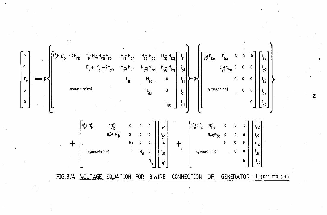
0 L~+ L" -2Mrb ~b Mry Myii Mrb Mrf Mbf Mrd Mbd MrG Mbq ir1 t.: +1.: 11,0 0 0 0 ir2 r b ro bo • 0 ~·+ ( -2M
y b .· yb Myf Mbf Myd Mbd M-M yq bq iil ~ +~ 0
yo bo 0 0 iy2
En =P Lff Mfd 0 if1 tP 0 0 0 if2
0 symme tri ea! Ldd 0 ~1
symmetrical 0 0 id2 "' "' 0 L ~1 0 iq2 qq
R•+R• r b .
. R' . . b 0 0 0 ir1 R'+R' ro bo 'R' bo 0 0 0 ir2
~.._ R" . b 0 0 0 iy1 RyffRbo 0 0 0 ~2
+ Rf 0 0 if1 + 0 0 0 if2
symmetrical Rd 0 id1 symmetrical 0 0 id2
Rq iq1 0 iq2
FIG. 3.14 VOLTAGE EQUATION FOR 3-WIRE CONNECTION OF GENERATOR- 1 (REF. FIG. 3.10)
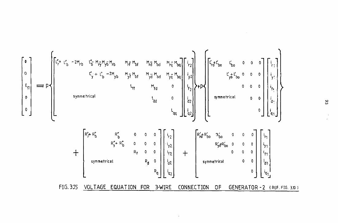
0 L.,.-1- ~ - 2M L'- M-M -M Hrf Hbf Hrd Mbd HrQ Mbq ir2 t: +t: t: 0 0 0 i r L b rb b rt yb rb ro bo bo r 1
0 r + t -2H Myf Hbf Hyd Mbd M-M iy2 t: + t: o 0 0 i y b yb yq bq yo bo y1
Ef2 =P Lff Mfd 0 if2 tP 0 0 0 if1
0 symmetrical Ldd 0
b2 symmetrical 0 0 id1 '"' w
0 L i 0 i qq q2 Q1
R''+ R'' r b R' b 0 0 0 ir2 R'+R' ro bo ~bo 0 0 0 ir1
R"+ R• y b 0 0 0 iy2. Ry&flbo 0 0 0 ~1
+ Rf 0 0 ifl + 0 0 0 i f1
symmetrical Rd 0 idl symmetrical 0 0 id!
Rq iQ2 0 i . ql.J
FIG.3.JS VOLTAGE EQUATION FOR 3-WIRE CONNECTION OF GENERATOR -2 I REF. FIG. 3.10 l
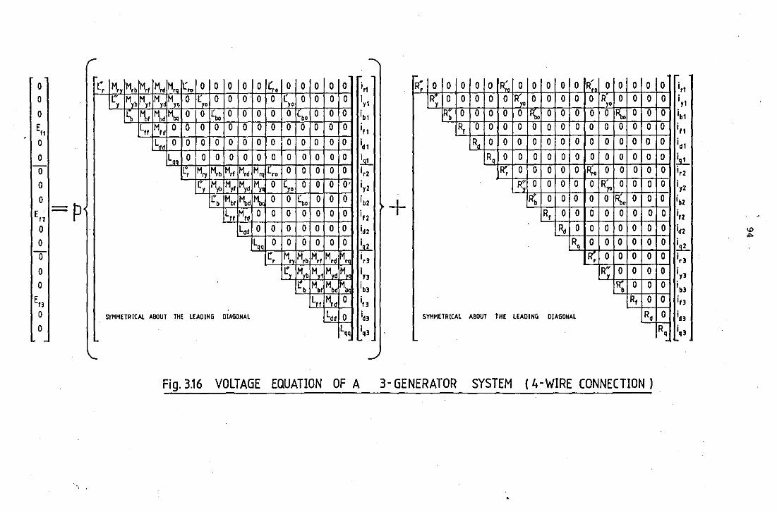
0 0
0
E,1 0
0
0 0
0
E,, = p 0
0 0
0
0
En 0
0
L", M,1
M,, M., M,d M., t:, 0 0 0 0 0 r.. 0 0 0 0 0 t:''
1 Mtb M
11 M1' M
10 0 t:, 0 0 0 0 0 [10 0 0 0 0
r, M,, M,d M00 o o rbo o o o o o 1L,, o o o Ltt Mfd 0 0 0 0 0 0 0 0 0 0 0 0 0
Lddoo oooooo ooo oo L, 0 0 0 0 0 0 0 0 0 0 0 0
1:, Mry M,, M., M,d M, l., 0 0 0 0 0
r
i~ i y1
ib1
., 1
i d1
!L
1:'1 ~b M11 M1d ~' 0 (10 0 0 0 0' i12
t, M,, 1'\,d Mbq 0 0 (,, 0 0 0
Lff M1d 0 0 0 0 0 0 0 i f2
Ldd 0 0 0 0 0 0 0
L.,OOOOOO i .:iL
~MHETRICAL ABOUT THE LEADING DIAGONAL
r, M" M,, M,, M,d M, i r3
t, M,, M,, M,d M,, in
r, M., M,dMh i,3
L11 M1d 0
Ldd 0 L,, ~ql
Fig, 3.16 VOLTAGE EQUATION OF A
r-!(, 0 0 0 0 0 R~ 0 0 0 0 0 R' 0 0 0 0
R, 0 0 0 0 0 R 'fO 0 0 0 0 0 R 0 0 0 yo R, 0 0 0 0 o I~ 0 0 0 0 o IR'" 0 0
R, 0 0 0 0 0 0 0 0 0 0 0 0 0
Rd 0 0 0 0 0 0 0 0 0 0 0 0
R, 0 0 0 0 0 0 0 0 0 0 0
1(, 0 0 0 0 0 R;, 0 0 0 0
R• n, 0 0 0 0 0 R" 0 0 0
+ IR'b 0 0 0 0 0 Rbo 0 0
R, 0 0 0 0 0 0 0
R.t 0 0 0 0 0 0
R• 0 0 0 0 0
IR', 0 0 0 0 RH 'v 0 0 0
If\ 0 0
R, 0
SYMMETRICAL ABOUT THE LEADING DIAGONAL Rd
3- GENERATOR SYSTEM ( 4-WIRE CONNECTION )
0 0
0
0
0
0 0
0
0
0
0
0
0
0
0
0
0
R, -
i r1 i y1
b1
11
d1
i
i
i
i .:9.!... i r2
i y2
b2
f2
d2
i
i
i
i
i r)
i
i
i
y)
b)
f)
i
i d)
q)
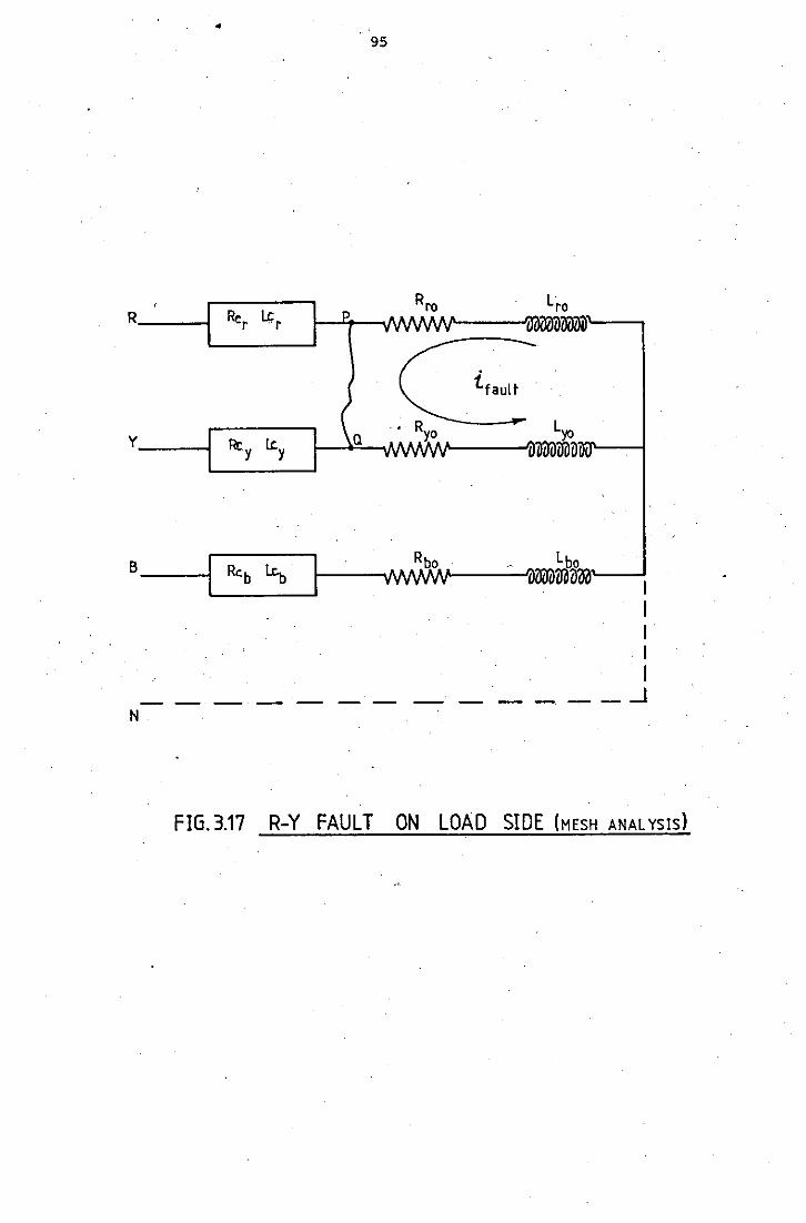
B __ -l
N
• 95
Rbo Lbo 1----IMf\MNf-' --'i)Wi)~Q3al'----l
I I I
. I . I
----- - ·- ._--- _j
FIG. 3.17 R-Y FAULT ON LOAD SIDE (MESH ANALYSIS)
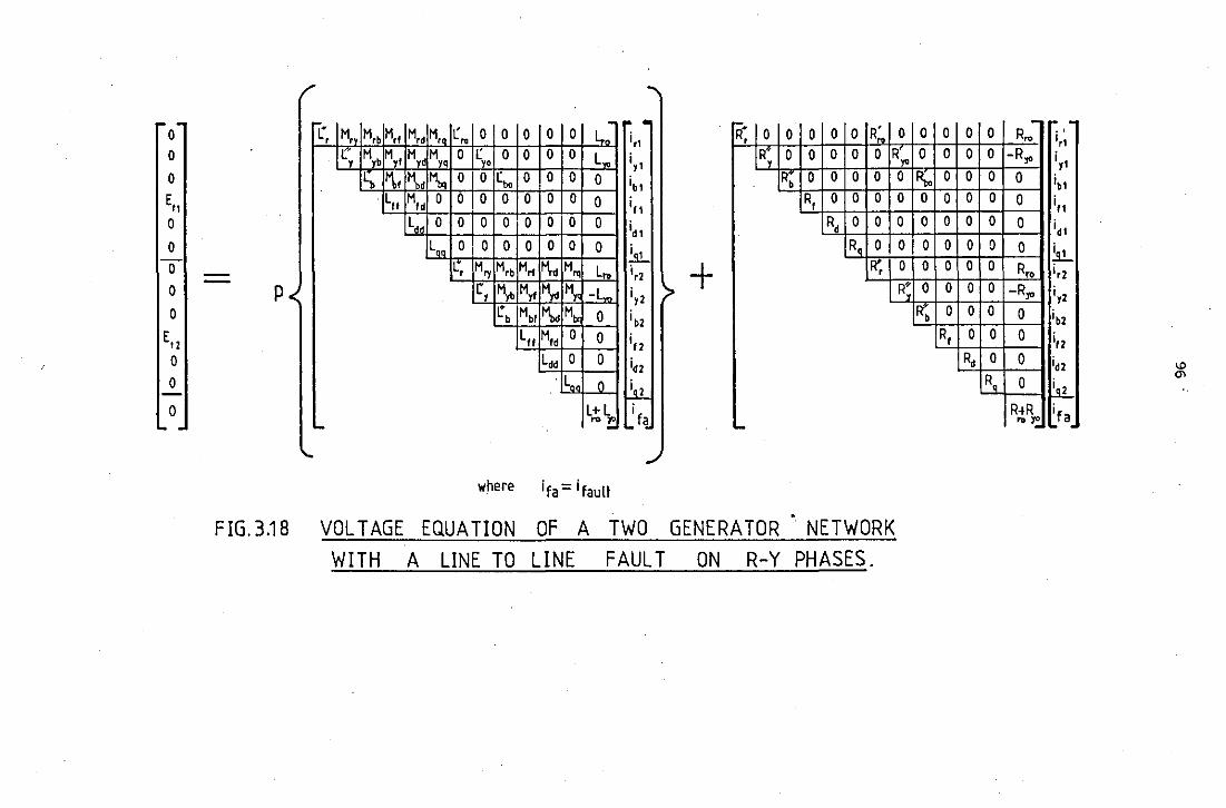
....
0 r-L' M, M,b M,, M,, M., r 0 0 0 0 0 L.: ~ .
' .. ir1
r-. R' R, 0 0 0 0 0 0 .. 0
0
[' M,b M,, M, M 0 r 0 0 0 0 Lw iy, y yq yo
11, 1'\,, Mbd I M, 0 0 ( 0 0 0 0 ib1 bo
R, 0 0 0 0 0 R,.
Rb 0 0 0 0 0
E,, . Lit M,. 0 0 0 0 0 0 0 0 i, 1 R, 0 0 0 0
0 L,, 0 0 0 0 0 0 0 0 id 1
R, 0 0 0
0
0 0 p 0
L" 0 I 0 0 0 0 0 0 !sL c, M., M,b Mrt M..t M., Lro ir2
< r, M,b Myt M,. I~ -Lw iy2 r Mbl I'\. Mb 0 ibl b
+ R, 0 0
IR'. 0
R•
E,l L, M,, 0 0 ;, 2
0 L,, 0 0 idl 0
0
. L, 0 ~ L+L I .... M> ! L. f~ ....
'-
where ita=itault
FIG.3.18 VOLT AGE EQUATION OF A TWO GENERA TOR NETWORK
WITH A LINE TO LINE FAULT ON R-Y PHASES.
0 0 0 0 0 0
R;., 0 0
0 0 0
0 0 0
0 0 0 0 0 0
0 0 0
IR'b 0 0
R, 0
R,
0 0
0
0
0
0 0
0
0
0
0
R,
. .. . R,. 0 0
'·• -R,. i,, 0 ib1
0 i,, 0 id1
0 !s.'.. R,, ir2
-R,. i,z 0 ibl 0 ;,2 0 idl 0 liol
R~R ifa .. >: L.'
"' "'
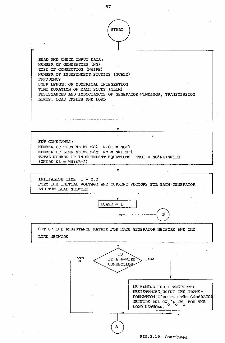
97
(START l
T READ AND CHECK INPUT DATA: NUMBER OF GENERATORS (NG) TYPE OF CONNECTION (NWIRE) NUMBER OF INDEPENDENT STUDIES (NCASE) FREQUENCY STEP LENGTH OF NUMERICAL INTEGRATION TIME DURATION OF EACH STUDY (TLIM) RESISTANCES AND INDUCTANCES OF GENERATOR WINDINGS, TRANSMISSION LINES, LOAD CABLES AND LOAD
SET CONSTANTS: NUMBER OF TORN NETWORKS: NCCT = NG+l NUMBER OF LINK NETWORKS~· NM = NWIRE-1 TOTAL NUMBER OF INDEPENDENT EQUATIONS NTOT = NG*NL+NWIRE (WHERE NL = NWIRE+2)
INITIALISE TIME T = 0.0 FORM THE INITIAL VOLTAGE AND CURRENT VECTORS FOR EACH GENERATOR AND THE LOAD NETWORK
~ I ICASE = 1 I
G SET UP THE RESISTANCE MATRIX FOR EACH GENERATOR NETWORK AND THE
LOAD NETWORK
YES ~ IT A 4 WIRE NO
CONNECTIO
DETERMINE THE TRANSFORMED RESISTANCEStUSING THE TRANS-FORMATION C RC fOR THE GENERATO NETWORK AND CW R CW FOR THE LOAD NETWORK.
0 0 0
8 FIG.3.19 Continued
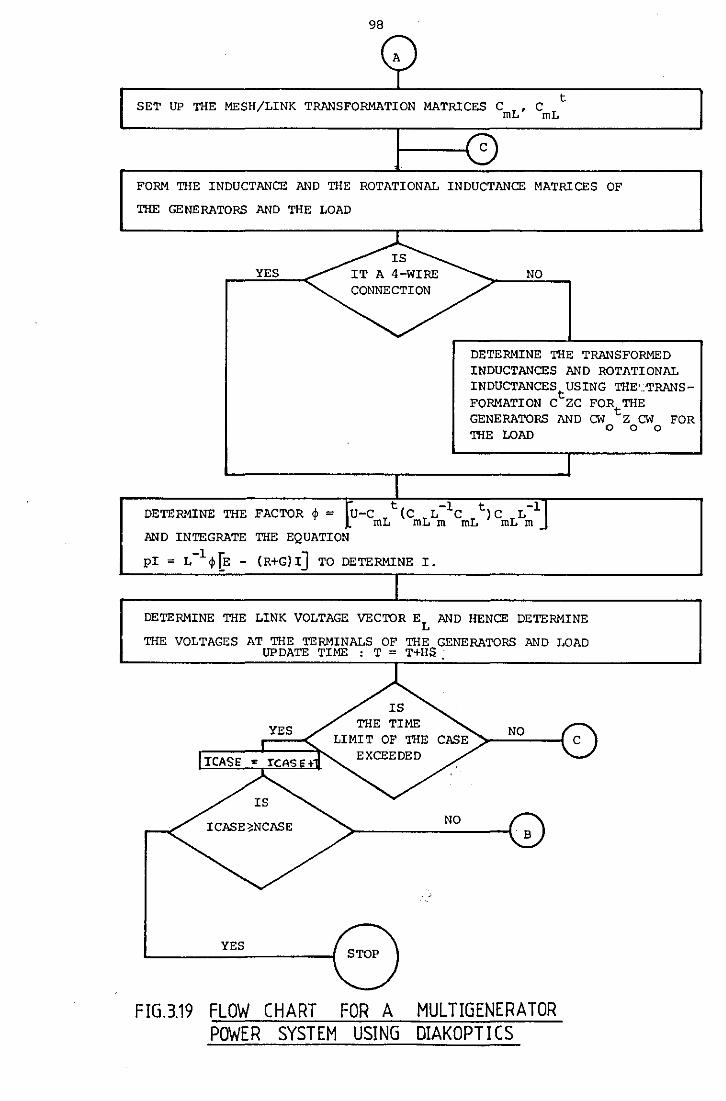
98
t SET UP THE MESH/LINK TRANSFORMATION MATRICES CmL' CmL
FORM THE INDUCTANCE AND THE ROTATIONAL INDUCTANCE MATRICES OF
THE GENERATORS AND THE LOAD
YES NO
DETERMINE THE TRANSFORMED INDUCTANCES AND ROTATIONAL INDUCTANCESt USING THE• __ TRANS
FORMATION C ZC FORtTHE GENERATORS AND CW Z CW FOR THE LOAD
0 0 0
DETERMINE THE FACTOR ~ = U-C Lt(C LL-1C t)C L-1 m rnmmL mLm
AND INTEGRATE THE EQUATION
pi = L -1 ~ fE - (R+G) I] TO DETERMINE I.
DETERMINE THE LINK VOLTAGE VECTOR EL AND HENCE DETERMINE
THE VOLTAGES AT THE TERMINALS OF THE GENERATORS AND LOAD UP DATE TIME : T = T+HS: ·
YES
FIG.3.19 FLOW CHART FOR A POWER SYSTEM USING
NO
MUL TIGENERA TOR DIAKOPTICS
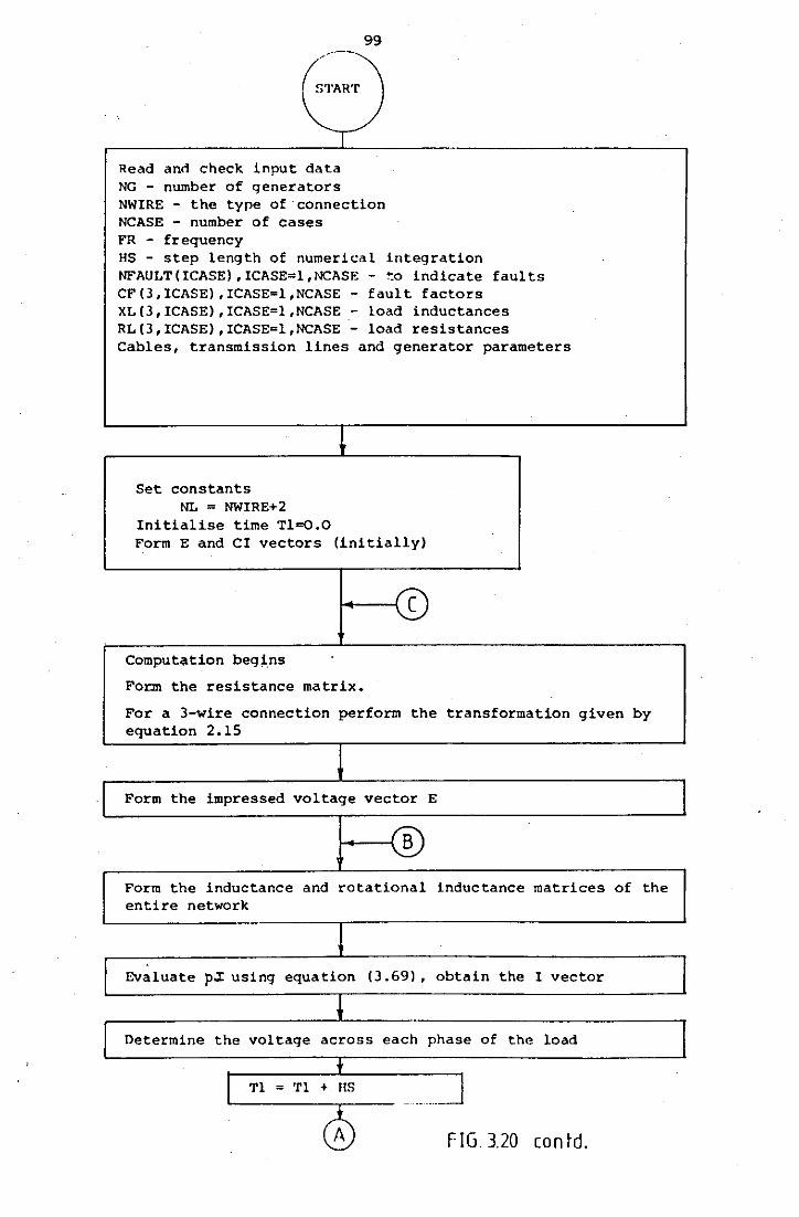
99 ---/
START )
Read ann check input data NG - number of generators NWIRE - the type of connection NCASE - number of cases FR - frequency HS - step length of numerical integration NFAULT(ICASE),ICASE=l,NCASE- to indicate faults CF(3,ICASE) ,ICASE=l,NCASE - fault factors XL ( 3, !CASE) , ICASE=l ,NCASE - load inductances RL(3,ICASE),ICASE=l,NCASE- load resistances Cables, transmission lines and generator parameters
.
Set constants NL = NWIRE+2
Initialise time Tl=O.O Form E and Cl vectors (initially)
c
Comput<ltion beg~ns
Fo~ the resistance matrix.
For a 3-wire connection perform the transformation given by equation 2.15
Form the impressed voltage vector E
B
Form the inductance and rotational inductance matrices of the entire network
Evaluate p.;r using equation (3 .69) , obtain the I vector
+ Determine the voltage across each phase of the load
t l Tl = Tl + llS --- _ _j
0 F JG. 3.20 con td.
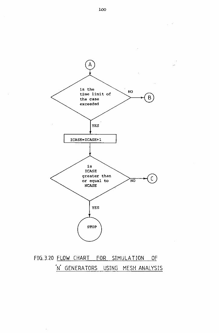
LOO
is the time limit of the case exceeded
YES
ICASE=ICASE+l
is !CASE
greater than or equal to
NCASE
YES
FIG. 3.20 FLOW CHART FOR SIMULA T!ON OF
'N' GENERATORS USING MESH ANALYSIS
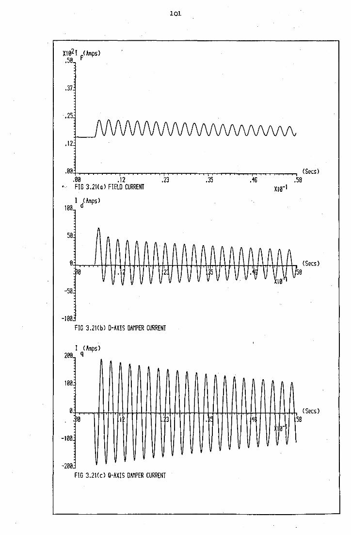
101
.37
.25
.12
.00'+.-~~~......,~~~~"'T""~~~,...,...,,...,-.~~~..,....,~~~.,....,.., (Secs) .00 .12 .23 .35 .16 .58
• FIG 3.2Ha> FIELD CURRENT
100_ I iAmps)
50
0 0 2
-50:
-100: FIG 3.21(b) D-AXIS DAMPER CURRENT
I <Amps> 200 q
100
-100
-200 FIG 3.21(c) Q-AXIS DAMPER CURRENT
(\
5 10~
V5a
(Secs)
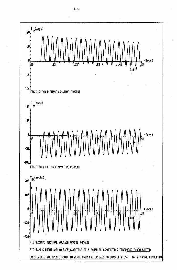
102
I CAmps) 100 r
50
0 <Secs) a .12 .23 ,,s .1 Vs a
m-1 -se
-100 FIG 3.2Hdl R-PHASE ARMAT~E CURRENT
I <Amps) 10a y
sa
0 <Secs) a 2 . s . 58
1 --sa
-100 FIG 3.2Hel Y-PHASE ARMAT~ CURRENT
20a VRN<Vollsl
100
0 <Secs) I • s 58
I 1 -100
-200 FIG 3.2HF l TERMINAL VOLTAGE ACROSS R-PHASE
FIG 3.21 CURRENT AND VOLTAGE WAVEFORMS OF A PARALLEl CONNECTED 2-GENERATOR POWER SYSTEM
ON STEADY STATE OPEN CIRCUIT TO ZERO POWER FACTOR LAGGING LOAD OF 0.6SmH FOR A 1-WIRE CONNECTIO
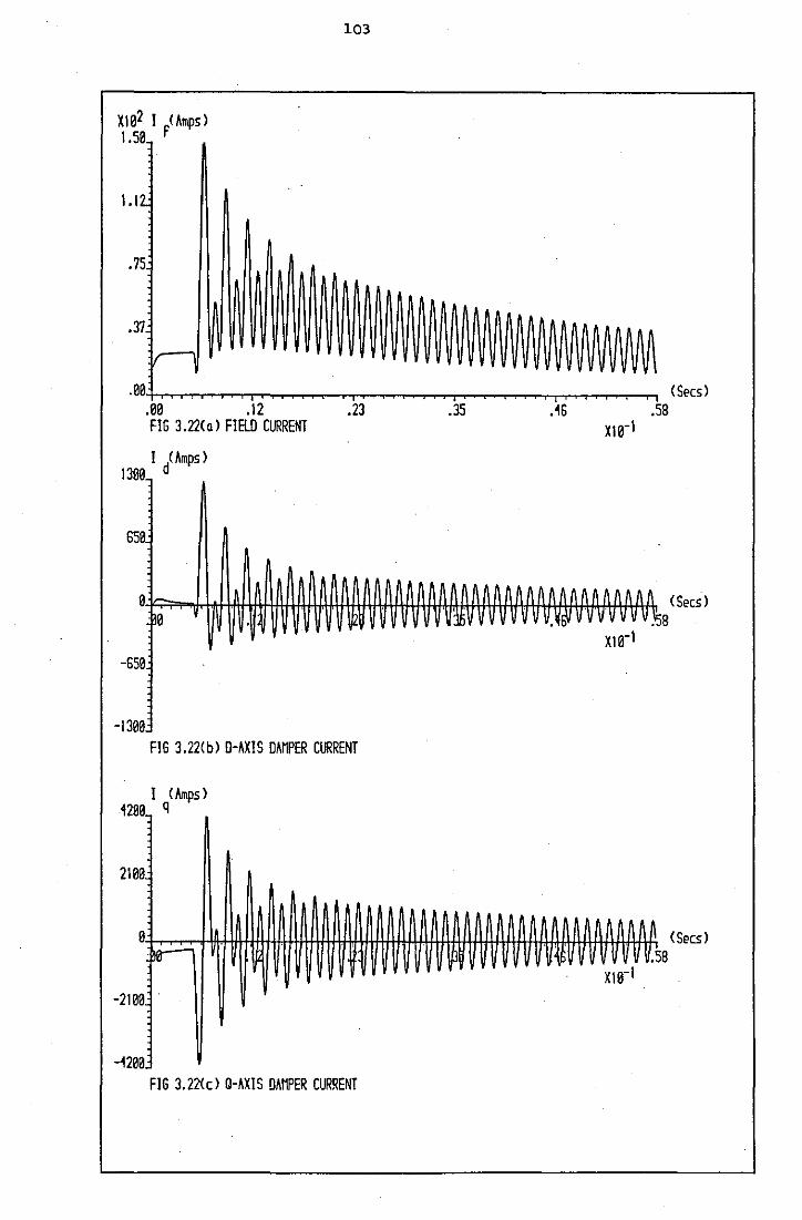
103
1.1
.75
.37
.001+-..~~~~,...,....,~~ ......... ~~.,...,_..,~...,......~""T-T~.,...,.-~~~......... (Secs) .00 .12 .23 .35 .'16 .58 FIG 3 .22< a l FIRD CURRENT
I iAmps) 1300
650
01~:;=;-..U,rJ.I,IW-U-1.1-l-f.l+l+\.j,U,\,~!mfWUU1i+UI.J.Ul.M~WWUW.f.A..A+\.AM <Secs l 0
-650
-1300 FIG 3.22<bl D-AXIS DAMPER CURRENT
I <Amps) 1200 q
2100
0
~
-2100
-1200 FIG 3.22<cl Q-AXIS DAMPER CURRENT
. 8
,\~I A <Secs)
(~~ .58 x1a-1
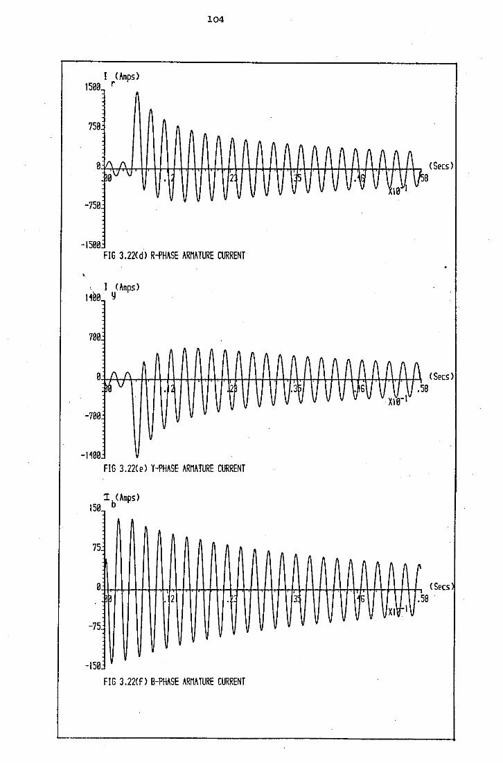
I (Amps) 1500 r
750
0 1\ (\
-750
-1500
104
2
FIG 3.22<dl R-PHASE ARMATURE CURRENT
·. I <Amps> 1100 y
700
(\ (\ (\
(\ 11 11 (\
0-t-f+ f\1+ "-J+-+t--H-1f+.J+t+f.-lr+t+t+t+Jr.J-r1;rf-\,-J.-\-+++t-f+J-+,f.-H4-/.-\ ( Secs ) ~ V .3 . 6 _
11 .58
V V X1'0-1'
-700
-1100 FIG 3.22(e) Y-PHASE ARMATURE CURRENT
75
I'
0 <Secs . 2 3 6 .58
X1 1
-75
-150
FIG 3.22<F> B-PHASE ARMATURE CURRENT
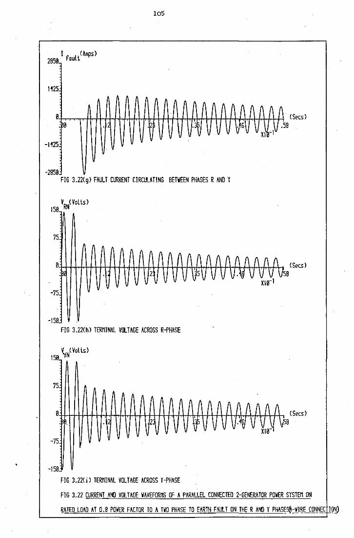
•
105
I F ll<Ampsl 2850 QU
1125_
(\ (\ 11 (\ (\
0'-:l-r.,...,-'f"T""f+-tt+H-if-.trl.,.frt+.J.+t+t++f-,t-,-h+-lf..H'-H-t+f+.\+t+-\rHHIIY < Secs J
V 58
V XI -lv 0 .3 .. 6
-1125
-2850 FIG 3.22(g) FAULT CURRENT CIRCULATING BETWEEN PHASES R AND Y
75
11 11 11 11 A 11 {\ (\(\(\
0-:t+++t+t+t+lr+t-+t+++tr+t-t+-t-r~:rH+t+++Ti+rnf+J~-Ti <Secs J 5 v v v V.~ v ~~0~ Vss 2
-75
-150 FIG 3.22<hl TERMINAL VOLTAGE ACROSS R-PHASE
V"N( Volls J 150 I
75
(\ (\ fl f\ A f\ 0-t+-1-H+++Ti+t+ii+i..-H,-t-+++t+.t-+t+-\rHrl-\--t-++t##f+rnl-h <Secs l
V V .4~ . V X10_\l IJSS V V
-75
-150 FIG 3.22<il TERMINAL VOLTAGE ACROSS Y-PHASE
FIG 3.22 CURRENT AND VOLTAGE WAVEFORMS OF A PARALLEL CONNECTED 2-GENERATOR POWER SYSTEM ON
RATED LOAD AT 0.8 POWER FACTOR TO A TWO PH\SE TO EARTH FAULT ON THE RAND Y PHASE~-:fi~~C IQ~
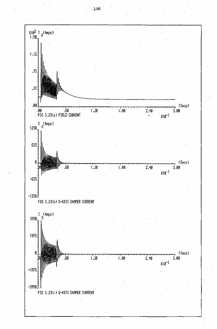
106
.60 1.20 FIG 3.23(a) FIELD CURRENT
I iAmps)
1.20
FIG 3.23(b) D-AXIS DAMPER CURRENT
.60 1.20
FIG 3.23(c) 0-AXIS DAMPER CURRENT
.80
.80
1.80
(Secs) .10 .00
.40
10
m-1
(Secs) .00
(Secs)
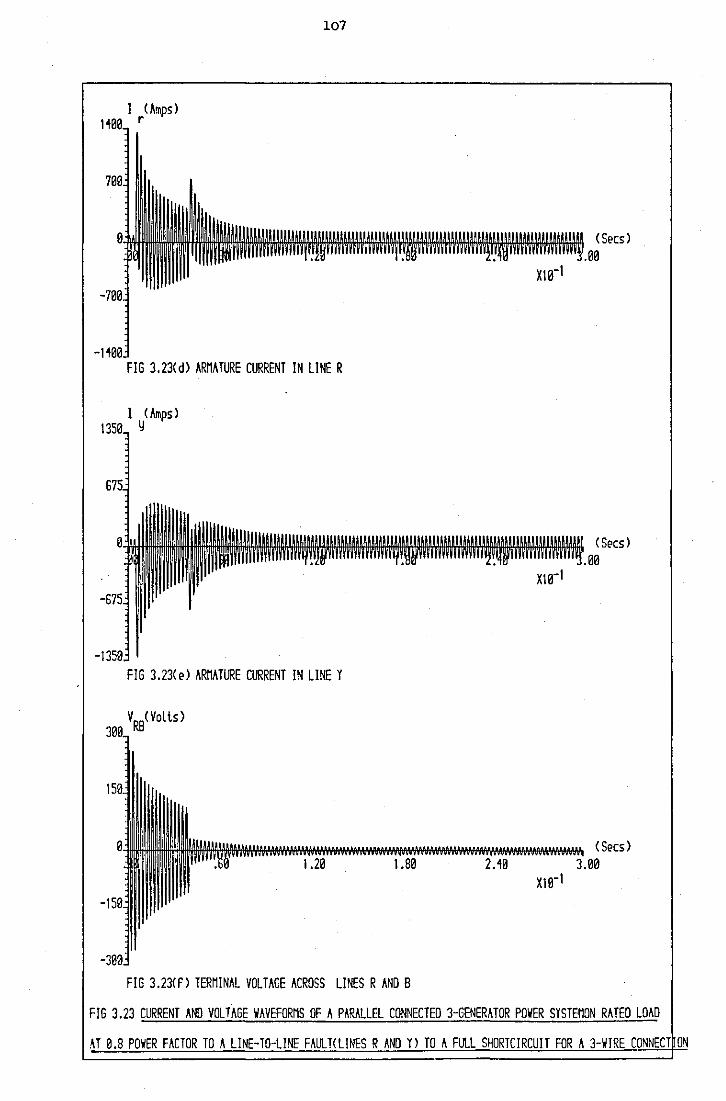
107
I <Amps> r
FIG 3.23(d) ARMATURE CURRENT IN LINE R
FIG 3.23(e) ARMATURE CURRENT IN LINE Y
1.20
FIG 3.23(f) TERMINAL VOLTAGE ACROSS LINES R AND 8
2.40
<Secs) .00
<Secs) .00
(Secs) 3.00
FIG 3.23 CURRENT AND VOLTAGE WAVEFORMS OF A PARALLEL CONNECTED 3-GENERATOR POWER SYSTEMON RATED LOAD
AT 0.8 POWER FACTOR TO A LINE-TO-LINE FAULT<LINES R AND Y> TO A FULL SHORTCIRCUIT FOR A 3-WJRE CONNECT ON
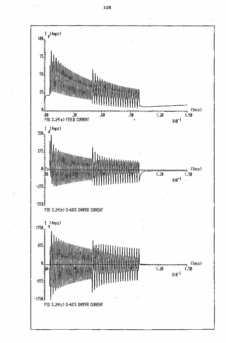
108
I I F<Ampsl
(Secs) 1.20 1.50
FIG 3.21(al FIElD CURRENT Xl0-l
(Secs) .20 1.50
Xl0-l
FIG 3.21(b) D-AXIS DAMPER CURRENT
(Secs) 1.20 1.50
Xl0-l
FIG 3.21(cl 0-AXIS DAMPER CURRENT
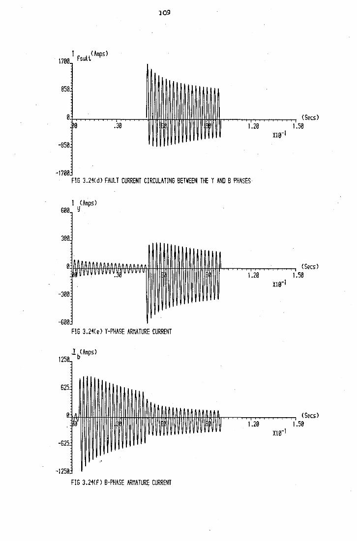
109
I faull<Ampsl
(Secs l 1.20 1.50
x10-1
FIG 3.24<dl FAULT CURRENT CIRCULATING BETWEEN THE Y AND B PHASES·
<Secs) 1.20 1.50
x1e-1
FIG 3.24(el Y-PHASE ARMATURE CURRENT
(Secs) 1.20 .50
x10-1
FIG 3.24<Fl B-PHASE ARMATURE CURRENT
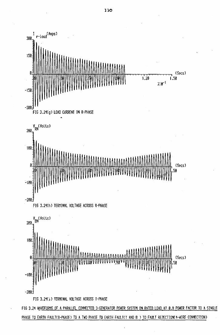
I l d(Ampsl r- oa
FIG 3.21(gl LOAD CURRENT IN R-PHASE •
110
FIG 3.21(hl TERMINAL VOLTAGE ACROSS R-PHASE
FIG 3.21(il TERMINAL VOLTAGE ACROSS Y-PHASE
(~a)
.20 1.50 ~;9-1
FIG 3.21 V~VEFORMS OF A PARALLEL CONNECTED 3-GENERATOR POWER SYSTEM ON RATED LOAD AT 0.9 POWER FACTOR TO A SINGLE
PHASE TO EARTH FAULT(B-PHASEl TO A TWO PHASE TO EARTH FAULT<Y AND B l TO FAULT REJECTION(1-WIRE CONNECTION>
111
CHAPTER 4
SIMULATION OF AN AC/DC 3-PHASE FULL-WAVE BRIDGE CONVERTER
Power conversion from AC to DC is often achieved by static
converters, using thyristors for controlled rectification or diodes
This_ ~~p_t<e_r_ d_e s_':"_ibe :._m_"_th_:ma tic a 1
models for both uncontrolled and c~ntrolled bridge converters, using ---~- ------
for uncontrolled rectification.
a tensor approach to define the different circuit equations which
apply as the pattern of device conduction and therefore the circuit -- ------------------------topology changes. The system considered comprises a·bridge converter ~---·--- --------supplied from a stiff 3-phase supply through a short length of cable,
possessing both resistance and inductance. Section 4.1 describes a
model for the diode bridge converter and this is extended in Section
4.3 to the case of a fully-controlled converter.
The network topology_ in both diode or thyristor circuits changes
continually with til!le, _an~ __ c_lassical solutions obtained by solving
the differential equations applied at each different state lead to an
unwieldy computer-based solution • For this reason, the tensor approach . - ----· ---- . developed by Kron16 •17 is used here to assemble and to solve automatically
the network equations. The program developed handles automatically ~------------· -----~- t • --
any changes in the state of the network and produces the relevant .-· ---------· -------- -
differential equations describing the_ network at each stage of the ------------ -----· ---
solution. The differential equations are solved numerically using ---- ------ - ---- . -- -·-- -- -· - --------- --- ....
the 4th-order Runge-Kutta integration routine.outlined in Appendix 2 ---- ------ -- -- ---- ----- - - - - -- - ----------and the solution processes for an uncontrolled and controlled bridge
converter are given respectively in sections 4.2 and 4.4.
4.1 System Equations of the Diode Bridge Model
A diode converter supplied via a cable from an infinite bus
112
is shown in Fig. 4.1. Two reference frames are required to solve
the system equations, these being the primitive or branch reference
frame and the mesh reference frame. The equations for both frames
have the same overall form and a fundamental requirement of the
analysis is that power is invariant between the two refe~ence frames20
•
4.1.1 The Primitive Reference Frame
The primitive reference frame is concerned with the unconnected
branches of the network as defined in Fig. 4.2(a}, and the corresponding
matrix branch voltage equation is given in Fig. 4.2(b}. Using Happs
notation20, this equation may be written in abbreviated form as
= (4.1}
where Eb is the impressed branch voltage vector, Vb is the branch
voltage vector, Ibis the branch current vector and ~band ~bare/
respectively the branch resistance and inductance matrices.
~As shown in Fig. 4.2(b) the impedance matrix. (~b + ~bpl has
a simple form, with the main diagonal elements being the self-impedances
of the various branches. In this type of matrix, any off-diagonal
elements would indicate mutual impedances between the different
branches, but in the circuit to be analysed these are all zero and
the impedance matrix degenerates to a diagonal matri~
4.1.2 The Mesh Reference Frame
The mesh reference frame is concerned with the meshes formed
when conducting diodes connect the load to the 3-phase lines, so
that the mesh equations are dependent on the various diode conduction
patterns. Thus, Fig. 4.3 shows the possible conduction meshes for
positive current in branch 'i', with Iil defining the mesh formed
113
when diodes o1
and o6
conduct, and Ii2
defining the mesh when diodes
o1
and o2
conduct. Since there are three· line currents, it follows
"that the maximum nwnber of possible conduction meshes is six. The
th . meshes are nwnbered such that the i mesh.'.corresponds to Di and
D. 1
conducting. ].-
Table 4.1 shows the ~~eri~g of the meshes for £!
the various conduction patterns~ At any particular instant, there
are a maximum of two conducting meshes_ (a complete short circuit of
the bridge due to Mode 3 operation is not considered). As an example,
consider conducting mesh 1 denoted by I11
in Fig. 4.3, with the
suffix i replaced by 1. Diodes o1
and o6 are forward biased. If
diode o2 becomes forward biased then mesh 2 commences conduction,
with the current denoted by I12
in Fig. 4.3. Mesh current I11
does not fall instantaneously to zero since there is inductance in the ___:_-------------- --
supply circuit, and meshes 1 and 2 conduct simultaneously until I11
decreases to zero, at which time mesh 1 is effectively removed from
the circuit • .. ----·--··
The abbreviated form of the mesh equation is
E +V = R I + L pi m m Dmlm mm m
(4.2)
where E is the impressed mesh voltage vector, V is the mesh voltage m m
vector (a· null vector in accordance with Kirchhoff's law), I is the m
mesh current vector and R and L are respectively the mesh resistance mm mm
and inductance matrices.
Equation (4.2) may be re-arranged in the state-variable form
pi m
-1 = L (E - R I ) mm m mmm
and integrated numerically to obtain a new I vector. m
(4. 3)
Thus a
step-by-step solution for the mesh currents may_be obtained. The
order of E , I , R and L is either one or two, depending on the mmnnn mm
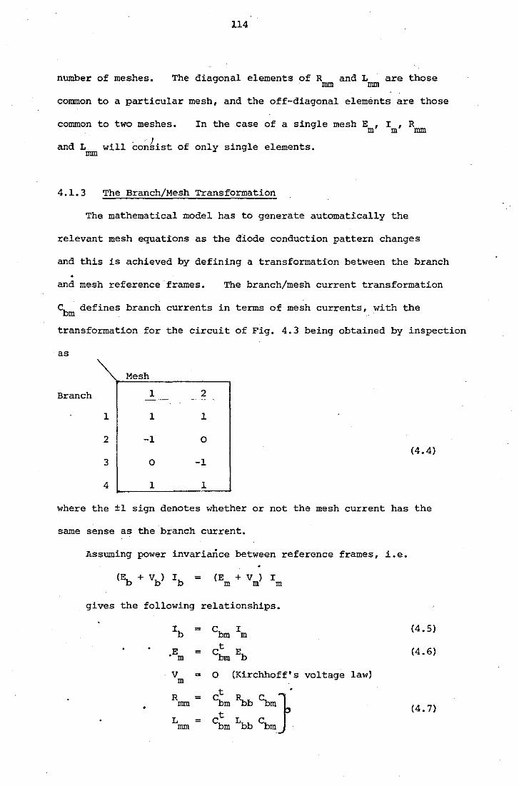
114
number of meshes. The diagonal elements of R and L are those mm mm
common to a particular mesh, and the off-diagonal elements are those
common to two meshes. In the case of a single mesh E , I , R m m mm
' ) and L. will consist of only single elements. mm
4.1. 3 The Branch/Mesh Transformation
The mathematical model has to generate automatically the
relevant mesh equations as the diode conduction pattern changes
and this is achieved by defining a transformation between the branch
and mesh reference frames. The branch/mesh current transformation
Cb defines branch currents in terms of mesh currents, with the m .
transformation for the circuit of Fig. 4.3 being obtained by inspection
as
Mesh
Branch 1 2
1 1 1
2 -1 0 (4. 4)
3 0 -1
4 1 1
where the ±1 sign denotes whether or not the mesh current has the
same sense as the branch current.
Assuming power invariaflce between reference frames, i.e.
= (E + V ) I m m m
gives the following relationships.
Ib = cbm I m (4. 5)
.Em = et Eb bm (4. 6)
V = m 0 (Kirchhoff' s voltage law)
R t •
= Cbm ~b ~m} mm
L = c~m Lbb cbm · mm
(4. 7)
115 I
t where cbm is the transpose of cbm·
To implement the model requires the automatic generation of
Cbm as the diode conduction pattern varies, as is described in
Section 4. 2. 1.
4.2 Solution Process for the Diode Bridge Model
A computer program based on the relationships given in Section 4.1
was developed to solve the equations for the converter. The numerical
solution proceeds with the following operations.
1) Form the branch resistance matrix ~b and the branch
inductance matrix ~b·
the simulation period.
These remain unchanged throughout
2) Form the mesh resistance matrix R and the mesh inductance mm
31
4)
5)
6)
7)
matrix L using equation (4.7}. mm
Determine E using equation (4.6}. m
Integrate equation (4.3) numerically, using the technique
---------------~ ~-described in Appendix 2 to obtain the new mesh current .::-vector I •
m
Determine Ib from equation (4.5).
Determine Vb using equation (4.1}.
The solution advances by one step, at the end of which --- -· ----- . --- ---- -·--- . - ---· ---------~-~--------------·-----~---"
a test is made for any change in the diode conduction -----------.._ -----~---~---------·-- ---------
pattern. Discontinuities are caused by diodes turning
off (current discontinuities) or by diodes turning on
(voltage discontinuities) and a discontinuity test procedure
is described in Section 4.2.2. If changes are detected,
the solution proceeds by:
(a) determining the time between the start of the step
and the first discontinuity, using linear interpolation;
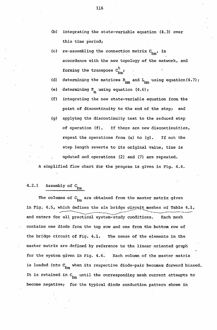
4.2.1
116
(b) integrating the state-variable equation (4.3) over
this time period;
(c) re-assembling the connection matrix Cbm' in
(d)
(el
(f)
accordance with the new topology of the network, and
t forming the transpose cbm;
determining the matrices R and L using equation(4.7); mm mm
determining E using equation (4.6); m
integrating the new state-variable equation from the
point of discontinuity to the end of the step; and
(g) applying the discontinuity test to the reduced step
of operation (f). If there are new discontinuities,
repeat the operations from (a) to (g). If not the
step length reverts to its original value, time is
updated and operations (2) and (7) are repeated.
A simplified flow chart for the program is given in Fig. 4.4.
Assembly of Cbm
The columns of Cbm are obtained from the master matrix given
in Fig. 4.5, which defines the six bridge circu:[,t meshes of Table 4.1,
-------~---- ------------·---- ------~ -and caters for all practical system-study conditions. Each mesh
contains one diode from the top row and one from the bottom row of
the bridge circuit of Fig. 4.1. The sense of the elements in the
master matrix are defined by reference to the linear oriented graph
for the system given in Fig. 4.6. Each column of the master matrix
is loaded into Cbm when its respective diode-pair becomes forward biased.
It is retained in Cbm until the corresponding mesh current attempts to
become negative; for the typical diode conduction pattern shown in
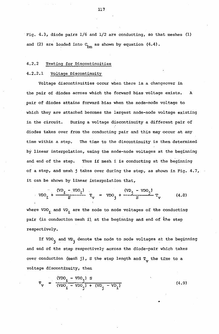
117
Fig. 4.3, diode pairs 1/6 and 1/2 are conducting, so that meshes (1)
and (2) are loaded into Cbm as shown by equation (4.4).
4.2.2 Testing for Discontinuities
4.2.2.1 Voltage Discontinuity
Voltage discontinuities occur when there is. a changeover in
the pair of diodes across which the forward bias voltage exists. A
pair of diodes attains forward bias when the node-node voltage to
which they are attached becomes the largest node-node voltage existing
in the circuit. During a voltage discontinuity a different pair of
diodes takes over from the conducting pair and this may occur at any
time within a step. The time to the discontinuity is then determined
by linear interpolation, using the node-node voltages at the beginning
and end of the step. Thus if mesh i is conducting at the beginning
of a step, and mesh j takes over during the step, as shown in Fig. 4.7,
it can be shown by linear interpolation that,
T V
= T V
(4. 8)
where VDO. and VD. are the node to node voltages of the conducting l. l.
pair (Jn conduction mesh i)_ at the beginning and end of the step
respectively.
If VDO. and VD. denote the node to node voltages at the beginning J J
and end of the step respectively across the diode-pair which takes
over conducti'On (mesli j I , s the step length and T the time to a V
voltage discontinuity, then
T V
= (VDOi
- VDO.) + J
(4. 9)
•
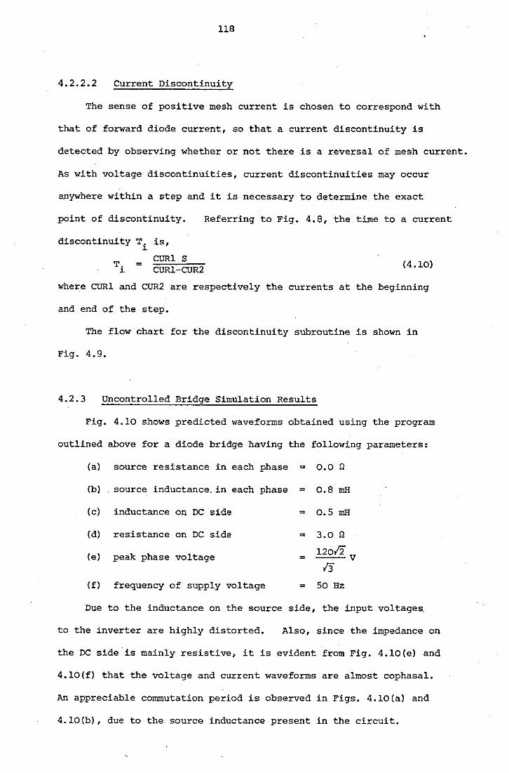
118
4.2.2.2 Current Discontinuity
The sense of positive mesh current is chosen to correspond with
that of forward diode current, so that a current discontinuity is
detected by observing whether or not there is a reversal of mesh current.
As with voltage discontinuities, current discontinuities may occur
anywhere within a step and it is necessary to determine the exact
point of discontinuity. Referring to Fig. 4.8, the time to a current
discontinuity Ti is,
= CURl S CUR1-CUR2
(4 .10)
where CURl and CUR2 are respectively the currents at the beginning
and end of the step.
The flow chart for the discontinuity subroutine is shown in
Fig. 4.9.
4.2. 3 Uncontrolled Bridge Simulation Results
Fig. 4.10 shows predicted waveforms obtained using the program
outlined above for a diode bridge having the following parameters:
(a) source resistance in each phase = 0.0 n
(b} source inductance. in each phase = 0.8 mH
(c) inductance on DC side = 0.5 mH
(d) resistance on DC side = 3.o n
(e) peak phase voltage = 12ofi V
13 (f) frequency of supply voltage = 50 Hz
Dt,1e to the inductance on the source side, the input voltages.
to the inverter are highly distorted. Also, since the impedance on
the DC side.is mainly resistive, it is evident from Fig. 4.10(e) and
4.10(f) that the voltage and current waveforms are almost cophasal.
An appreciable commutation period is observed in Figs. 4.10(a) and
4.10(b), due to the source inductance present in the circuit.
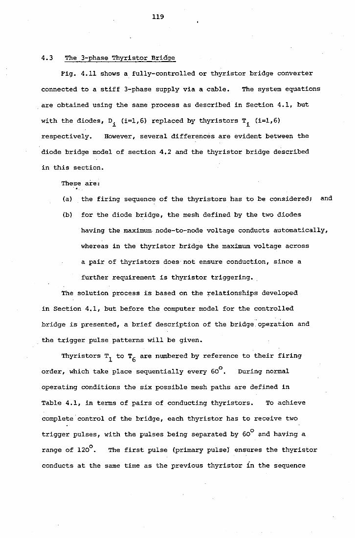
119
4.3 The 3-phase Thyristor Bridge
Fig. 4.11 shows a fully-controlled or thyristor bridge converter
connected to a stiff 3-phase supply via a cable. The system equations
are obtained using the same process as described in Section 4.1, but
with the diodes, Di (i=l,6) replaced by thyristors Ti (i=l,6)
respectively. However, several differences are evident between the
diode bridge model of section 4.2 and the thyristor bridge described
in this section.
These are: •
(a) the firing sequence of the thyristors has to be considered; and
(b) for the diode bridge, the mesh defined by the two diodes
having the maximum node-to-node voltage conducts automatically,
whereas in the thyristor bridge the maximum voltage across
a pair of thyristors does· not ensure conduction, since a
further requirement is thyristor triggering.
The solution process is based on the relationships developed
in Section 4.1, but before the computer model for the controlled
bridge is presented, a brief description of the bridge operation and
the trigger pulse patterns will be given.
Thyristors T1 to T6 are numbered by reference to their firing
order, which take place sequentially every 60°. During normal
operating conditions the six possible mesh paths are defined in
Table 4.1, in terms of pairs of conducting thyristors. To achieve
complete control of the bridge, each thyristor has to receive two
trigger pulses, with the pulses being separated by 60° and having a
range of 120°. The first pulse (primary pulse) ensures the thyristor
conducts at the same time as the previous thyristor in the sequence
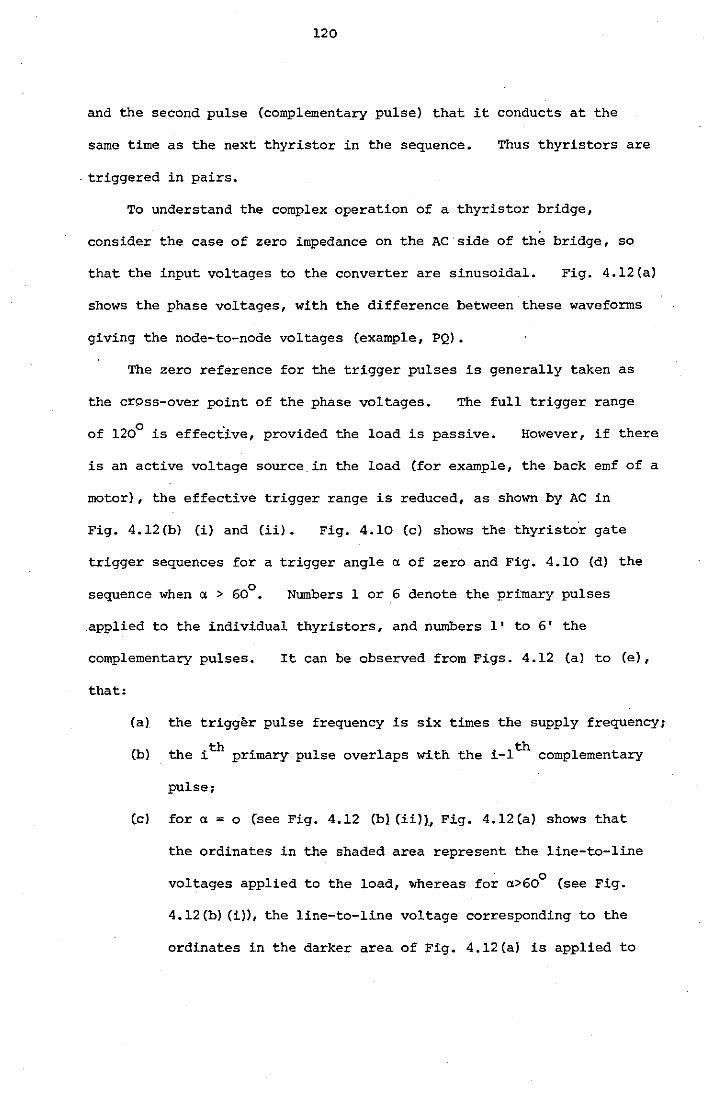
120
and the second pulse (complementary pulse) that it conducts at the
same time as the next thyristor in the sequence • Thus thyristors are
. triggered in pairs.
To understand the complex operation of a thyristor bridge,
consider the case of zero impedance on the AC side of the bridge, so
that the input voltages to the converter are sinusoidal. Fig. 4.12 (a)
shows the phase voltages, with the difference between these waveforms
giving the node-to-node voltages (example, PQ).
The zero reference for the trigger pulses is generally taken as
the cross-over point of the phase voltages. The full trigger range
of 120° is effective, provided the load is passive. However, if there
is an active voltage source in the load (for example, the back emf of a
motor), the effective trigger range is reduced, as shown by AC in
Fig. 4.12(b) (i) and (ii). Fig. 4.10 (c) shows the thyristor gate
trigger sequences for a trigger angle a of zero and Fig. 4.10 (d) the
h 600. sequence w en a > Numbers 1 or 6 denote the primary pulses
applied to the individual thyristors, and numbers 1' to 6' the
complementary pulses. It can be observed from Figs. 4.12 (al to (e),
that:
(a) the trigger pulse frequency is six times the supply frequency;
(b) the ith primary pulse overlaps with the i-lth complementary
pulse;
(cl for a = o (see Fig. 4.12 (bl (ii)J, Fig. 4.12 (a) shows that
the ordinates in the shaded area represent the line-to-line
voltages applied to the load, whereas for a>60° (see Fig.
4.12 (b) (i)), the line-to-line voltage corresponding to the
ordinates in the darker area of Fig. 4.12(a) is applied to
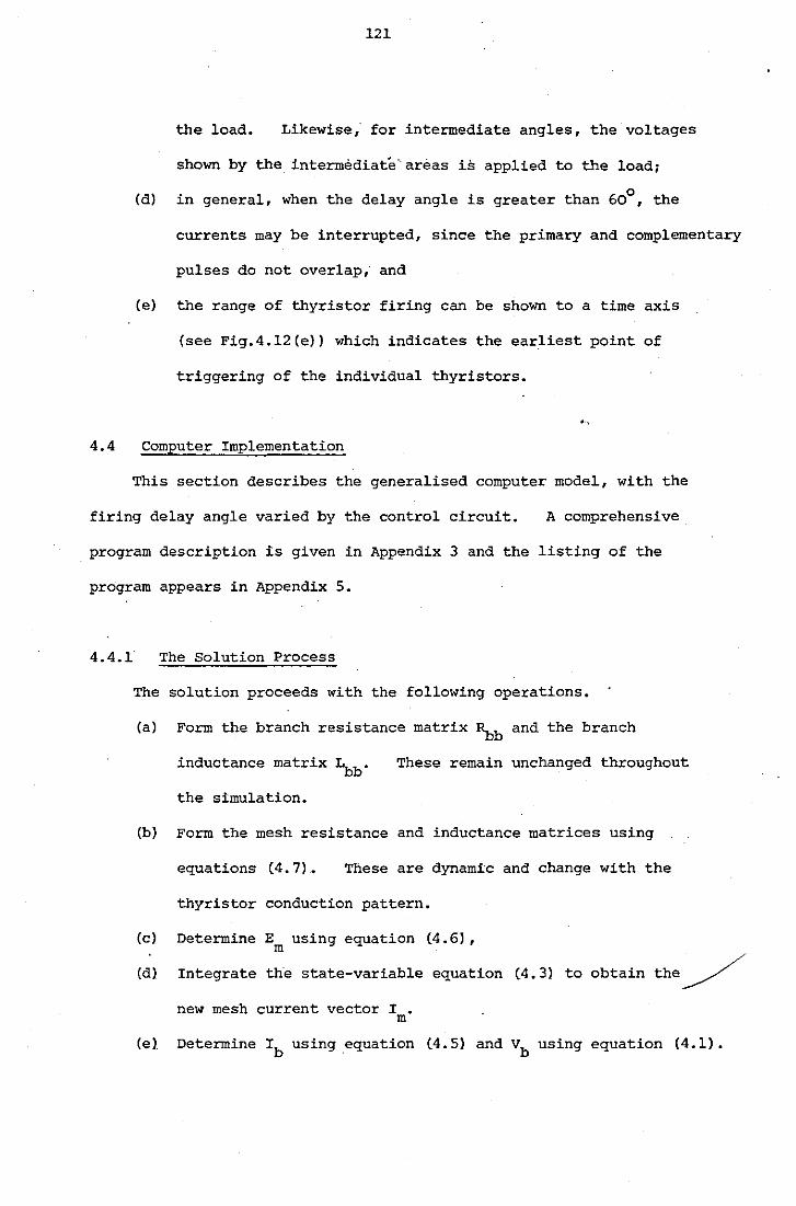
121
the load. Likewise; for intermediate angles, the voltages
shown by the. intermediate·· areas is applied to the load;
(d) in general, when the delay angle is greater than 60°, the
currents may be interrupted, since the primary and complementary
pulses do not overlap, and
(e) the range of thyristor firing can be shown to a time axis
(see Fig.4.12(e)) which indicates the earliest point of
triggering of the individual thyristors.
·--,
4.4 Computer Implementation
This section describes the generalised computer model, with the
firing delay angle varied by the control circuit. A comprehensive
program description is given in Appendix 3 and the listing of the
program appears in Appendix 5.
4.4.1 The Solution Process
The solution proceeds with the following operations.
(a) Form the branch resistance matrix ~b and the branch
inductance matrix ~b· These remain unchanged throughout
the simulation.
(b) Form the mesh resistance and inductance matrices using
equations (4.7). These are dynamic and change with the
thyristor conduction pattern.
(c) Determine E using equation (4.6), m
(d) Integrate the state-variable equation (4.3) to obtain the/
new mesh current vector I . m
(el. Determine Ib using equation (4.5) and vb using equation (4.1).
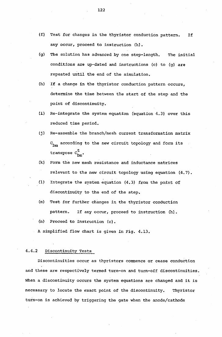
4.4.2
122
(f) Test for changes in the thyristor conduction pattern. If
any occur, proceed to instruction (h).
(g) The solution has advanced by one step-length. The initial
conditions are up-dated and instructions (cl to (g) are
repeated until the end of the simulation.
(h) If a change in the thyristor conduction pattern occurs,
determine the time between the start of the step and the
point of discontinuity.
(i) Re-integrate the system equation (equation 4.3) over this
reduced time period.
(j) Re-assemble the branch/mesh current transformation matrix
Cbm according to the new circuit topology and form its
t transpose cbm.
(kl Form the new mesh resistance and inductance matrices
relevant to the new circuit topology using equation (4.7).
(1) Integrate the system equation (4.3) from the point of
discontinuity to the end of the step.
(m) Test for further changes in the thyri-stor conduction
pattern. If any occur, proceed to instruction (h) •
(n) Proceed to instruction (c).
A simplified flow chart is given in Fig. 4.13.
Discontinuity Tests
Discontinuities occur as thyristors commence or cease conduction
and these are respectively termed turn-on and turn-off discontinuities.
When a discontinuity occurs the system equations are changed and it is
necessary to locate the exact point of the discontinuity. Thyristor
turn-on is achieved by triggering the gate when the anode/cathode
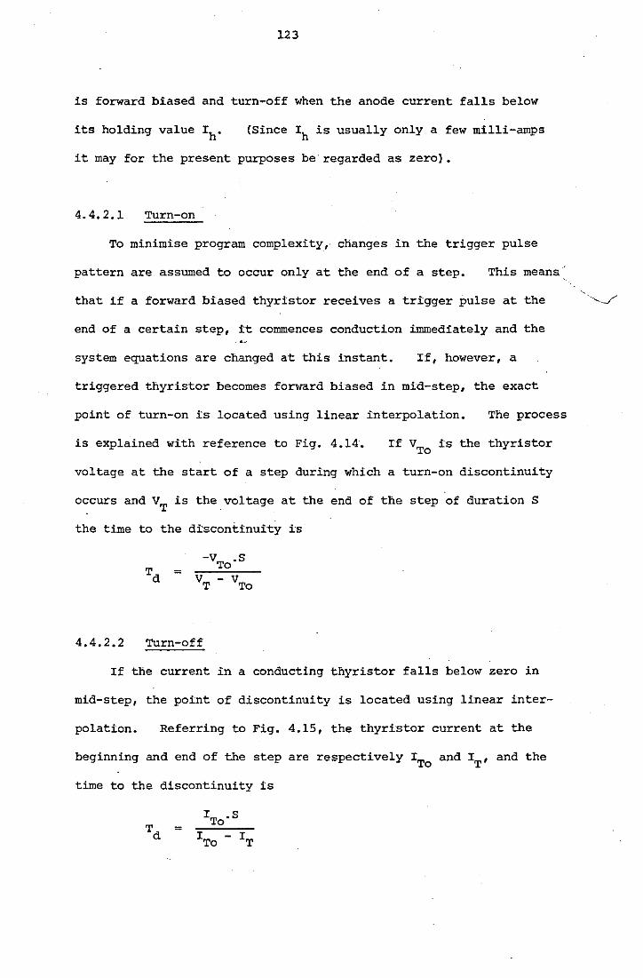
123
is forward biased and turn-off when the anode current falls below
its holding value Ih. (Since Ih is usually only a few milli-amps
it may for the present purposes be· regarded as zero}.
4.4.2.1 Turn-on
To minimise program complexity, changes in the trigger pulse
pattern are assumed to occur only at the end of a step. This means
that if a forward biased thyristor receives a trigger pulse at the
end of a certain step, it commences conduction immediately and the
system equations are changed at this instant. If, however, a
triggered thyristor becomes forward biased in mid-step, the exact
point of turn-on is located using linear interpolation. The process
is explained with reference to Fig. 4.14. If VTo is the thyristor
voltage at the start of a step during which a turn-on discontinuity
occurs and VT is the voltage at the end of the step of duration S
the time to the discontinuity is
4.4.2.2 Turn-off
If the current in a conducting thyristor falls below zero in
mid-step, the point of discontinuity is located using linear inter-
polation. Referring to Fig. 4.15, the thyristor current at the
beginning and end of the step are respectively ITo and IT' and the
time to the discontinuity is
=
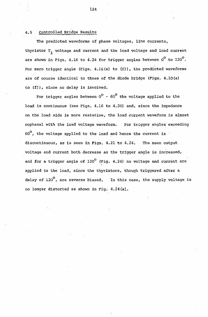
124
4.5 Controlled Bridge Results
The predicted waveforms of phase voltages, line currents,
thyristor T1
voltage and current and the load voltage and load current
0 0 are shown in Figs. 4.16 to 4.24 for trigger angles between 0 to 120 •
For zero trigger angle (Figs. 4.16(a) to (f)), the predicted waveforms
are of course identical to those of the diode bridge (Figs. 4.10(a)
to (f)), since no delay is involved.
For trigger angles between 0° - 60° the voltage applied to the
load is continuous (see Figs. 4.16 to 4.20) and, since the impedance
on the load side is more resistive, the load current waveform is almost
cophasal with the load voltage waveform. For trigger angles exceeding
60°, the voltage applied to the load and hence the current is
discontinuous, as is seen in Figs. 4.21 to 4.24. The mean output
voltage and current both decrease as the trigger angle is increased,
and for a trigger angle of 120° (Fig. 4.24) no voltage and current are
applied to the load, since the thyristors, though triggered after a
0 delay of 120 , are reverse biased. In this case, the supply voltage is
no longer distorted as shown in Fig. 4.24(a[.
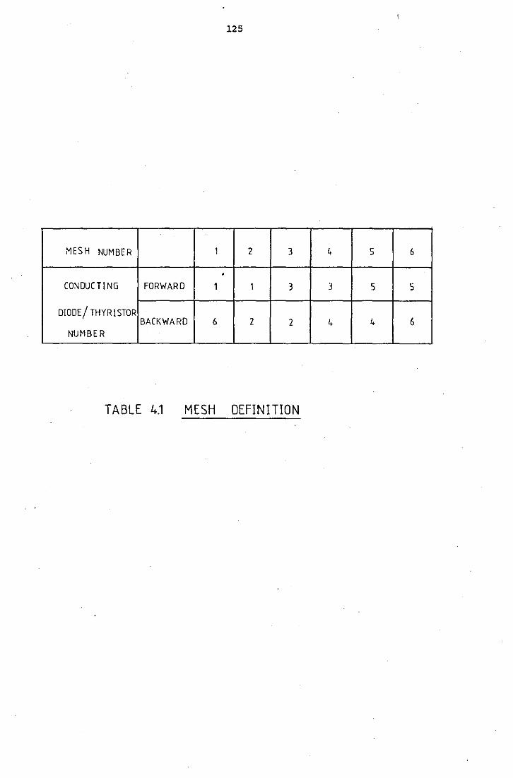
125
MESH NUMBER 1 2 3 4 5 6
. CONDUCTING FORWARD 1 1 3 3 5 5
DIODE/ THYRISTOR BACKWARD 6 2 2 4 4 6
NUMBER
TABLE 4.1 MESH DEFINITION
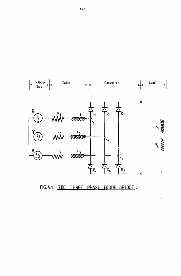
126
I· Infinite ·I• Cable Load bus ·I· Converter + ·I
FIG.4.1 THE THREE PHASE DIODE BRIDGE.
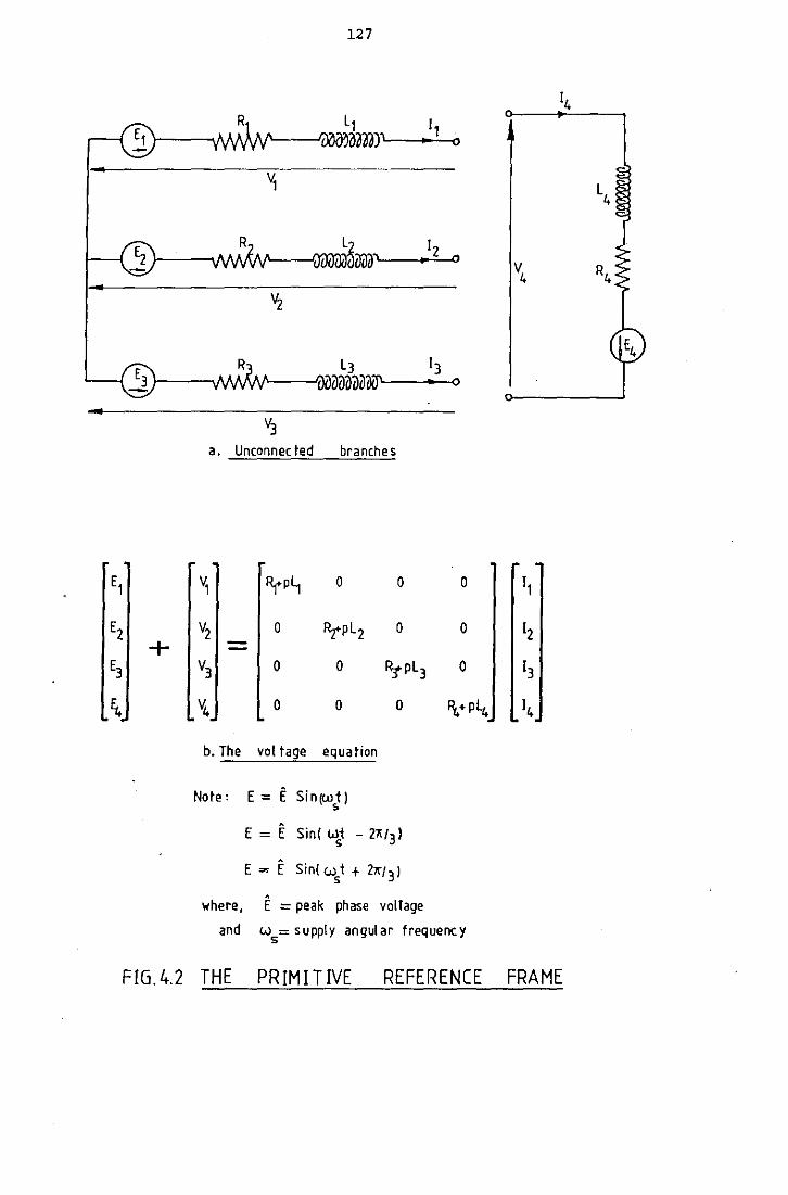
127
14
L1 11 3o-a4)1 • 0
V, L4
1z 0 • \
a. Unconnected branches
E1 ~ 'YP~ 0 0 0 11
Ez Vz 0 fltPLz 0 0 1z +
E3 v3 0 0 RtPL3 0 13
fi. v4 0 0 0 Re.· pl4 14
b. The vol tage equation
Note: E = E Sin(wt) &
E = E Sin( w~ - 2X/3l
E = E Sin( wst + 2-.:1 31
where, i': ==peak phase voltage
and w =supply angular frequency 5
F!G.4.2 THE PRIMITIVE REFERENCE FRAME
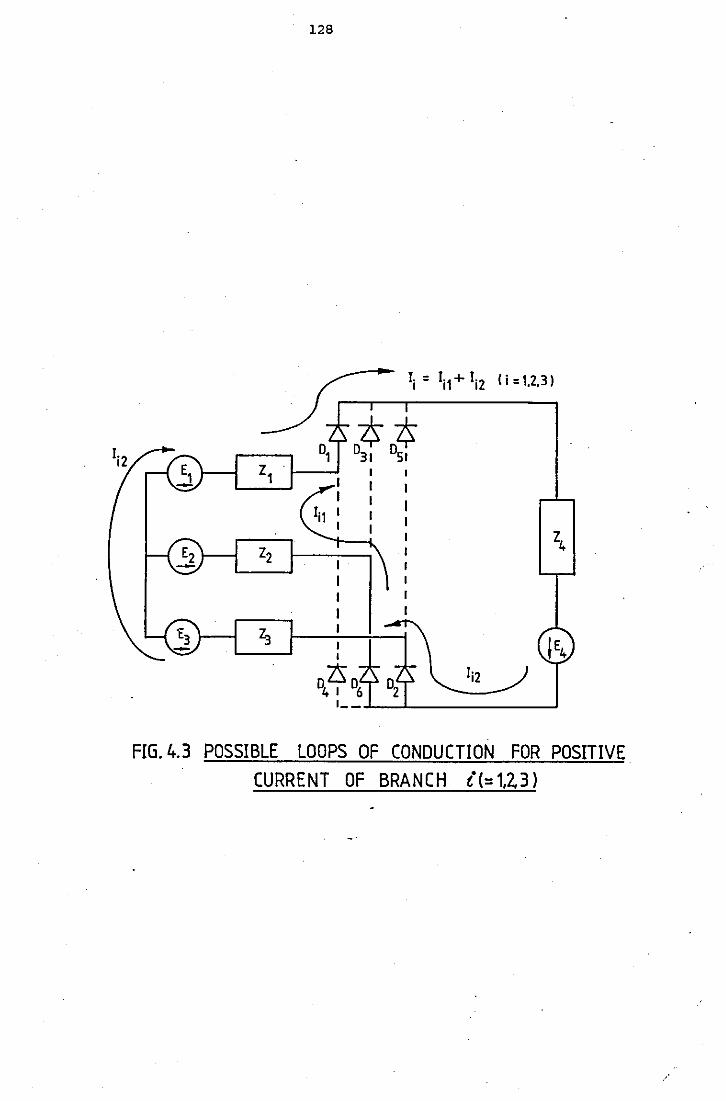
128
FIG. 4.3 POSSIBLE LOOPS OF CONDUCTION FOR POSITIVE
CURRENT OF BRANCH t"(= 1,2,3 l
/
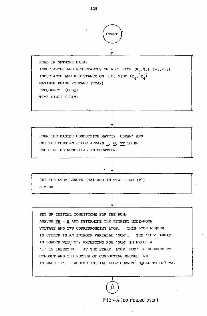
129
....--..
' ( START r
READ IN NETWORK DATA:
INDUCTANCES AND RESISTANCES ON A.C. SIDE (R.,X.) ,j=1,2,3) J J
INDUCTANCE AND RESISTANCE ON D.C. SIDE (R4
, x4
1
MAXIMUM PHASE VOLTAGE (VMAX)
FREQUENCY (FREQ)
TIME LIMIT (TLIM)
FORM THE MASTER CONDUCTION MATRIX 'CBRAN' AND
SET THE CONSTANTS FOR ARRAYS H, G, TT TO BE -USED IN THE NUMERICAL INTEGRATION.
'
SET THE STEP LENGTH (S~) AND INITIAL TIME (T1!
s = s~
SET UP INITIAL CONDITIONS FOR THE RUN:
ASSUME VB = E AND DETERMINE THE HIGHEST NODE-NODE - -VOLTAGE AND ITS CORRESPONDING LOOP. THIS LOOP NUMBER
IS STORED IN AN INTEGER VARIABLE 'NUM'. THE 'ICL' ARRAY
IS LOADED WITH O's EXCEPTING ROW 'NUM' IN WHICH A
. '1' IS INSERTED. AT THE START, LOOP 'NUM' IS ASSUMED TO
CONDUCT AND THE NUMBER OF CONDUCTING MESHES 'NM' IS MADE I 1 I • ASSUME INITIAL LOOP CURRENT EQUAL TO 0.1 mA.
0 FIG 4.4 ( contihued over)
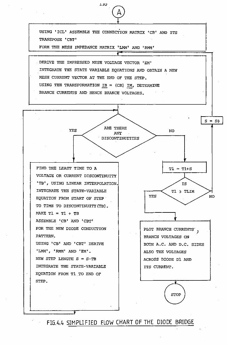
USING ' ICL' ASSEMBLE THE CONNECTION MATRIX 'CB' AND ITS
TRANSPOSE 'CBT'
FORM THE MESH IMPEDANCE MATRIX 'LMM' AND 'RMM'
DERIVE THE IMPRESSED MESH VOLTAGE VECTOR 'EM'
INTEGRATE THE STATE VARIABLE EQUATIONS AND OBTAIN A NEW
MESH CURRENT VECTOR AT THE END OF THE STEP.
USING THE TRANSFORMATION .!!! = (CB! IM, DETERMINE
BRANCH CURRENTS AND HENCE BRANCH VOLTAGES.
FIND THE LEAST TIME TO A
ARE THERE ANY
DISCONTINUITIES
VOLTAGE OR CURRENT DISCONTINUITY
'TB', USING LINEAR INTERPOLATION.
INTEGRATE THE STATE-VARIABLE
EQUATION FROM START OF STEP
TO TIME TO DISCONTINUITY (TB) •
MAKE Tl = Tl + TB
ASSEMBLE 'CB' AND 'CBT'
FOR THE NEW DIODE CONDUCTION
PATTERN.
USING 'CB' AND 'CBT' DERIVE
'LMM', 'RMM' AND 'EM'.
NEW STEP LENGTH S = S-TB
INTEGRATE THE STATE-VARIABLE
EQUATION FROM Tl .TO END OF
STEP.
NO
YES
PLOT BRANCH CURRENTS' )
BRANCH VOLTAGES ON
BOTH A.C. AND D.C. SIDES
ALSO THE VOLTAGES
ACROSS DIODE Dl AND
ITS CURRENT.
FIG.4.4 SIMPLIFIED FLOW CHART OF THE DIODE BRIDGE
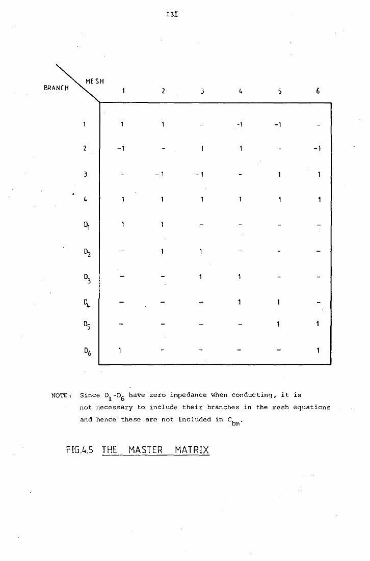
131
MESH BRANCH 2 3 4 5 6
-1 -1
2 -1 -1
3 -1 -1
4 1
01
02
03
q, 1 1
Ds 1 1
06
NOTE: Since o1
-o6
have zero impedance when conducting, it is
not necessary to include their branches in the mesh equations
and hence these arc not included in Cbm·
FIG.4.5 THE MASTER MATRIX
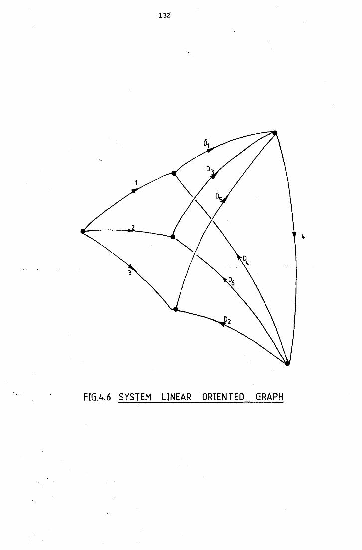
132"
4
FIG.4. 6 SYSTEM LINEAR ORIENTED GRAPH
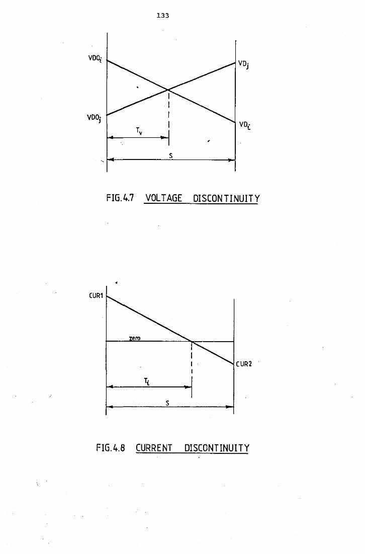
VD~
VDO· J
CUR1
133
s
FIG.4.7 VOLTAGE DISCONTINUITY
•
s
FIG.4.8 CURRENT DISCONTINUITY
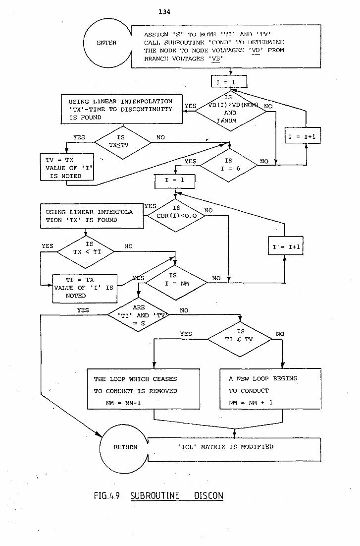
134
/\SS IGN Is I '1'0 BO'l'll I 'l'I I /\NI) I 'I'V I
CALl. SlJIIROU'I'lNE 'CO Nil' '1'0 I >1-:'I'I·:HM I NI·: TilE NODE '1'0 NODE VOL'l'AGJ·:S 'VD' FROM BRANCII VOLTAGES 'VIl'
USING LINEAR INTERPOLATION 'TX'-TIME TO DISCONTINUITY IS FOUND
NO
NO VALUE OF 'I'
IS NOTED
USING LINEAR INTERPOLATION 'TX' IS FOUND
YES
TI = TX VALUE OF 'I'
NOTED
YES
NO I = I+l
NO
THE LOOP WHICH CEASES A NEW LOOP BEGINS
TO CONDUCT IS REMOVED TO CONDUCT
NM = NM-l NM = NM + l
'I CL' MATRIX If, MODIFIED
FIG.4 9 SUBROUTINE DISCON
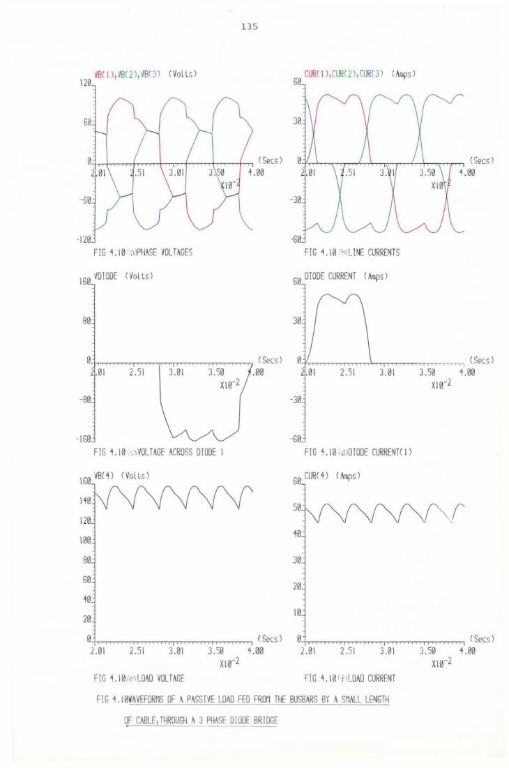
~B( 1 ) 1 ~B(2 ) 1 ~B( 3 l (Volts) 120
60
135
CUR( 1 ) I CUR( 2) I rUR( 3) (Amps ) 60
-+r.-f-r:-r...,....,..t-r-r""TT"Tit:-:-r-r-t,....,.--,-rtT'"""T""'I-r-t-...,.., ( Secs ) ( Secs ) 1.00 4.00
· 120 -60 FIG U 0 ~tlPHASE VOLT AGES FIG 4 . 10 '-.) Ll NE CURRENTS
160 ~DIODE <Volts) 60 DIODE CURRENT (Amps>
80
0-+-r-,.-,---..T"T'-:,......,.....,.....-n,..,.......,.-.,.--,r-:-r,.-,-....,.....,......, ( Secs ) -fr-.-'T"""T'"..,...,.-rr-.....-r-..,_,_n--<-.--,.......,....,"T"T"T",...,.........,.., ( Secs ) .01 2.51 .00 3.01 3.50 1.00
x1e-2 -80 -30
-160 -60 FIG 1.10 .\VOLTAGE ACROSS DIODE 1 FIG 1.10 tHO IODE CURRENT< 1)
160 VB( 1) (Volls) 60 CUR< 1) (Amps>
110 50 r 120
100 10
80 30
60 20
10
20 10
0 (Secs) 0 <Secs> 2.01 2.51 3.01 3.50 1.00 2.01 2.51 3.01 3.50 1.00
x10-2 x1e-2 FIG 1.10 e)LOAD VOLTAGE FIG 1.10 t1LOAD CURRENT
FIG 1.10WAVEFORMS OF A PASSIVE LOAD FED FROM THE BUSBARS BY A SMALL LENGTH - --
OF CABLE1TH~OUGH A 3 PHASF DIODE BRIDGE
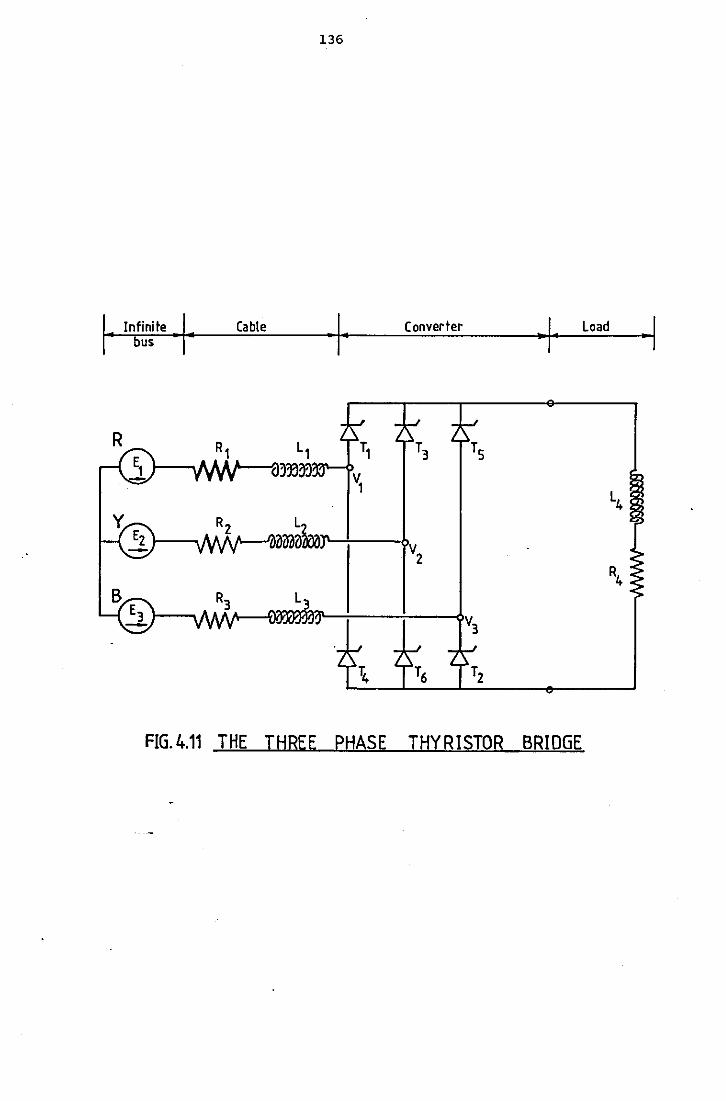
136
I· Infinite , I· Cable I· Load bus
Converter . I
FIG.4.11 THE THREE PHASE THYRISTOR BRIDGE
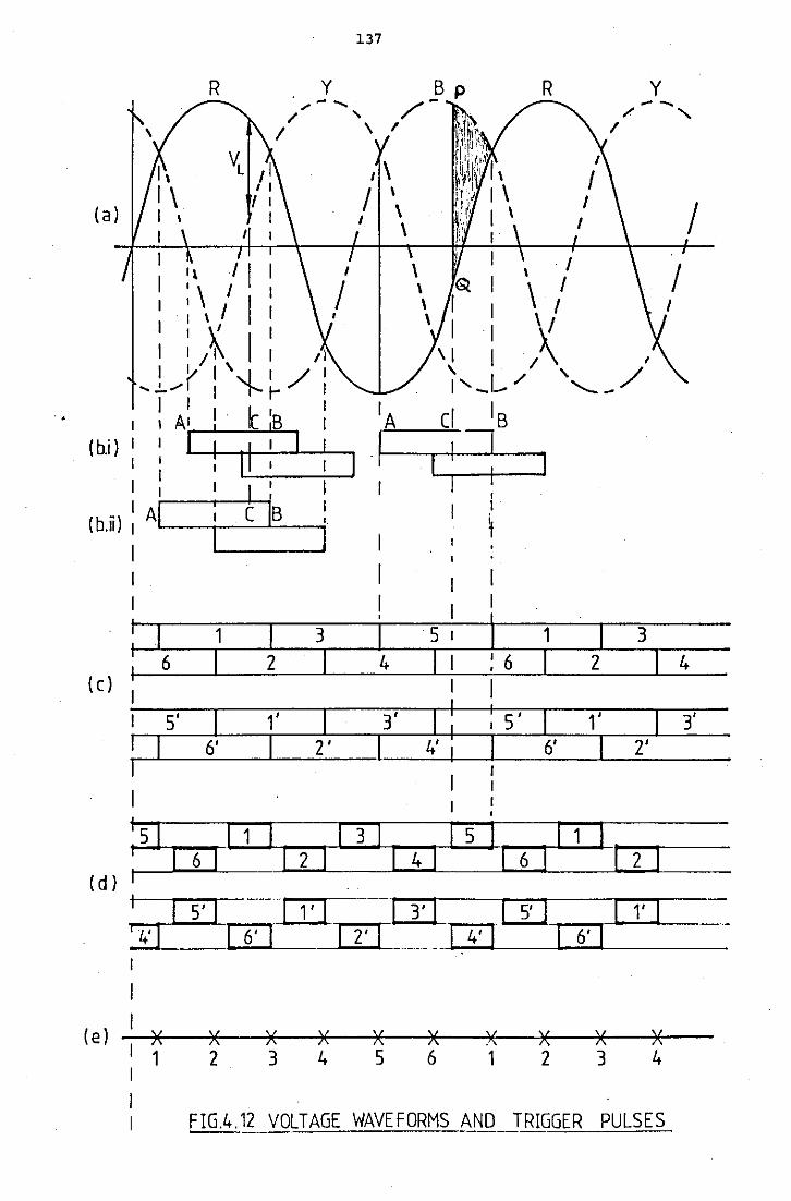
..
137
R y R y --..
'
(a) I ll I I I \ I
I I ' I I 1 \ I : \ I I
I I \'
I I/~ I I tl I (' I '.._1 1 / I
-..!.. ...- I .,..._ t- I I I I ,_ I I
1 I AI 1 · l. 18 I
(b.i) I I I I I I I I : 1 '-'-1 -:---..---'
I I I I : 1 b.U l : AI : c Is I
I I I
' I I \ I \I I /\ I ,,_1... .. ./ '..,__- /
1A cl 1s
. ''-'-----"'!...: J I I
~
I 1 3 I 5 I 1 3
6 I 2 I 4 I I 6 I 2 I 4 (c)
,.....-LI_51
----=-61 _ __,1'--1
--=-}-~ _[_31
---'4'---1, +--: -----~-; _ 5 _~ -'6'---1 _,.,_I --=-21 __ 3~_
:si Id I : I
I I 141
1
(e) )( 1
6ll1112ll3ll411sll6ll1112
5 I I I 11 I -I 3 I I I 51 I I 11 I
X 2
I 61 I I 2 I I -- --_I 41 I I 61 I
X )( X )( 3 4 5 6
X )( 1 2
X 3
X 4
FIG.4.12 VOLTAGE WAVEFORMS AND TRIGGER PULSES
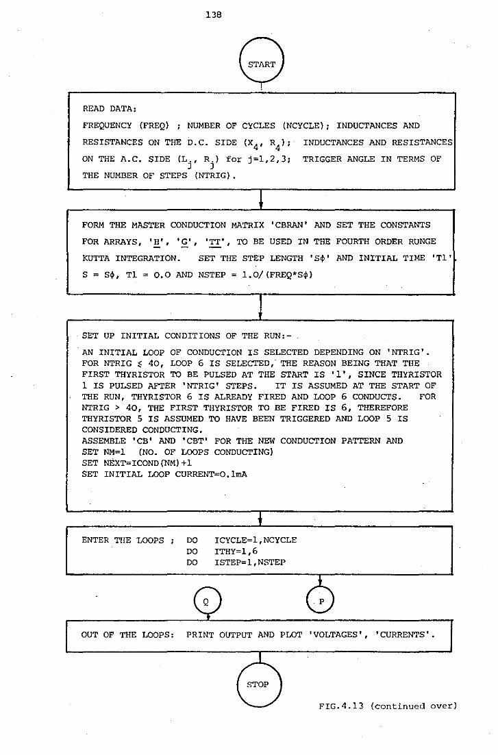
138
READ DATA:
FREQUENCY (FREQ) ; NUMBER OF CYCLES (NCYCLE); INDUCTANCES AND
RES I STANCES ON THE D.C. SIDE (X4, R4); INDUCTANCES AND RESISTANCES
ON THE A.C. SIDE (Lj, Rj) for j=l,2,3; TRIGGER ANGLE IN TERMS OF
THE NUMBER OF STEPS (NTRIG) .
FORM THE MASTER CONDUCTION MATRIX 'CBRAN' AND SET THE CONSTANTS
FOR ARRAYS, I H', '£'I 'TT' I TO BE USED IN THE FOURTH ORDER RUNGE
KUTTA INTEGRATION. SET THE STEP LENGTH 'S~' AND INITIAL TIME 'Tl'
S = S~, Tl = 0.0 AND NSTEP = 1.0/ (FREQ*S~)
SET UP INITIAL CONDITIONS OF THE RUN:-
AN INITIAL LOOP OF CONDUCTION IS SELECTED DEPENDING ON 'NTRIG'. FOR NTRIG ~ 40, LOOP 6 IS SELECTED; THE REASON BEING THAT THE FIRST THYRISTOR TO BE PULSED AT THE START IS '1', SINCE THYRISTOR 1 IS PULSED AFTER 'NTRIG' STEPS. IT IS ASSUMED AT THE START OF THE RUN, THYRISTOR 6 IS ALREADY FIRED AND LOOP 6 CONDUCT$. FOR NTRIG > 40, .THE FIRST THYRISTOR TO BE FIRED IS 6, THEREFORE THYRISTOR 5 IS ASSUMED TO HAVE BEEN TRIGGERED AND LOOP 5 IS CONSIDERED CONDUCTING. ASSEMBLE 'CB' AND 'CBT' FOR THE NEW CONDUCTION PATTERN AND SET NM=l (NO. OF LOOPS CONDUCTING} SET NEXT=ICOND (NM) +1 SET INITIAL LOOP CURRENT=O.lmA
i ENTER THE LOOPS ; DO ICYCLE=l,NCYCLE
DO ITHY=l,6 DO ISTEP=l, NSTEP
Q G OUT OF THE LOOPS: PRINT OUTPUT AND PLOT 'VOLTAGES', 'CURRENTS'.
FIG.4.13 (continued over)
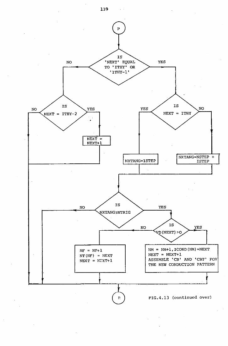
NO
NO
IS
NEXT = ITHY-2
NO
139
YES
NEXT= NEXT+l
IS 'NEXT' EQUAL TO 'ITHY' OR
'ITHY-1'
IS
XTANG~NTRIG
NF = NF+l NT(NF) = NEXT NEXT = NC:XT+l
G
YES
NO
YES
IS NO
NEXT = ITHY
YES
NXTANG=NSTEP + !STEP
YES
NM = NM+l,ICOND(NM)=NEXT NEXT = NEXT+l ASSEMBLE 'CB' AND 'CBT' FOR THE NEW CONDUCTION PATTERN
FIG.4.13 (continued over)
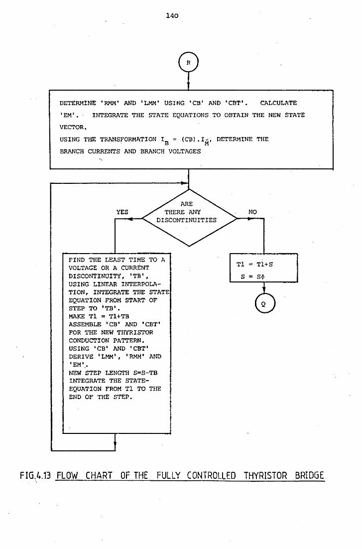
140
DETERMINE 'RMM' AND 'LMM' USING 'CB' AND 'CBT'. CALCULATE
'EM'. INTEGRATE THE STATE EQUATIONS TO OBTAIN THE NEW STATE
VECTOR.
USING THE TRANSFORMATION IB = (CB) .IM, DETERMINE THE
BRANCH CURRENTS AND BRANCH VOLTAGES '•
YES
FIND THE LEAST TIME TO A VOLTAGE OR A CURRENT DISCONTINUITY, 'TB', USING LINEAR INTERPOLATION, INTEGRATE THE STATE EQUATION FROM START OF STEP TO 1 TB'. MAKE Tl = Tl+TB ASSEMBLE 'CB' AND 'CBT' FOR THE NEW THYRISTOR CONDUCTION PATTERN. USING 'CB' AND 'CBT' DERIVE 'LMM', 'RMM' AND 'EM'.• NEW STEP LENGTH S=S-TB INTEGRATE THE STATEEQUATION FROM Tl TO Tire END OF THE STEP.
NO
Tl = Tl+S
s = s~
FIG.4.13 FLOW CHART OF THE FULLY CONTROLLED THYRISTOR BRIDGE
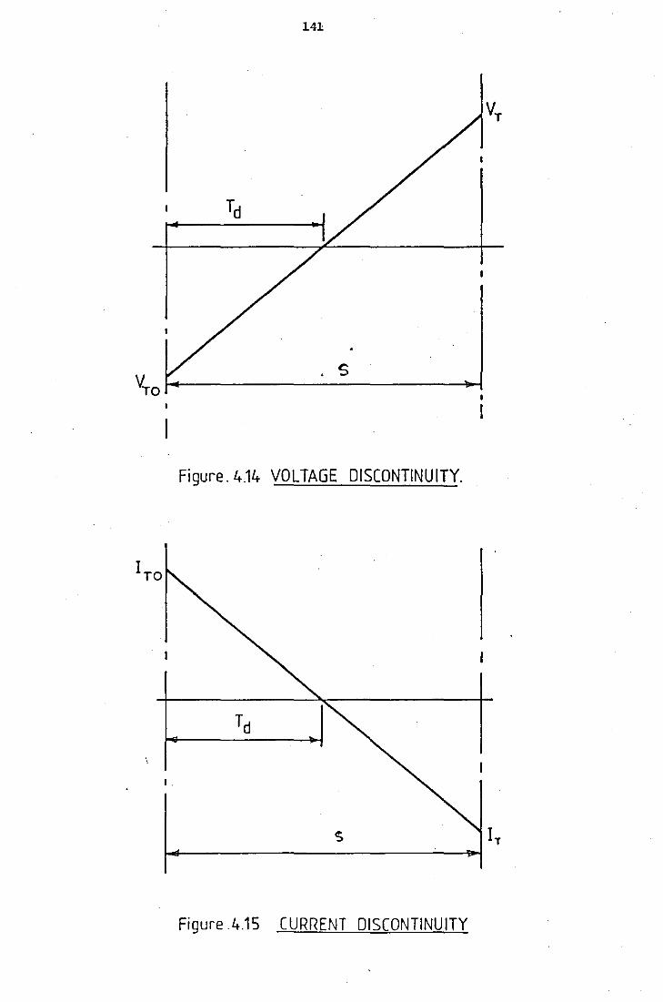
141
Figure. 4.14 VOLTAGE DISCONTINUITY.
Figure 4.15 CURRENT DISCONTINUITY
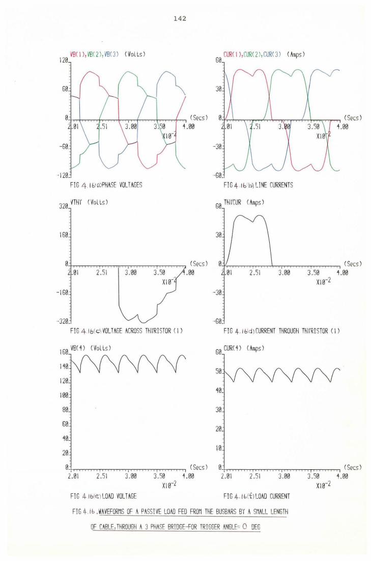
142
VB< 1 ) 1 VB< 2 ) 1 VB< 3 ) ( Vo lls ) CUR< 1 ),CUR( 2 ) 1 CUR< 3 ) ( Amps ) 1~ ~
-+-rr-+r-r--,,..,...,...,..f-,-r,,..--,-,Jfr-,-r-,:-r-rf,...,.......,--rtT"'T""T""'1.......,f.-"n"1. ( Secs ) ( Secs ) 4.00 4.00
-120 ·G0 FIG 4 I b' roPHASE VOLT AGES FIG 4 t b b) L1 NE CURRENTS
320 VTHY <Volls> GB THYCUR <Amps>
B-t-rr-'T'T'T""-r-r-,...,...,"'T'T"Tl;rT'T"l-r-T"-.--r--r-r.,..,...,....,'"'T"""T"~ ( Secs ) B-JL.r-r..--.-..,..,...,..rrn--.--'1,--,..,..,.......,..-,--,,_..,.,..,...-.,....-r-T-,..,. ( Secs ) .Bl 2.51 3.0B .0B 3.00 3.50 4 .BB
x10-2 -1G0 -3B
-320 -GB FIG 4 lbtc\VOLTAGE ACROSS THYRI STOR ( 1) FIG 4 I/, d l CURRENT THROUGH THYR I STOR ( 1 >
1G0 VB( 4) (Volls> GB CUR< 4 > (Amps)
14B 5B
120
tea- 40
8B 30
GB-20
4B
2B 10 '
0 (Secs) 0 2.01 2.51 3.00 3.50 4.00 2.01 2.51 3.00
xte-2 FIG 4-tbfe) LOAD VOLTAGE FIG 4. I l:.ft J LOAD CURRENT
FIG 4 tb .WAVEFORMS OF A PASSIVE LOAD FED FROM THE BUSBARS BY A SMALL LENGTH
OF CABLE, THROUGH A 3 PHASE BRIDGE-FOR TRIGGER ANGLE= 0 DEG
(Secs) 3.50 4.00
X10-2
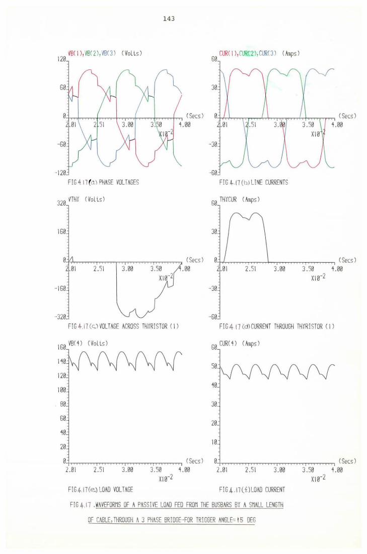
~B< 1 ), vB<2l ,VB(3) <Volls) 120
143
CUR< 1 ),CU~' 2), CUR< 3) <Amps ) 60
30
· -h-T-.t.-r...,....,...,.-r,-r.,,........-t-.-r,~f,-,-,-,,...,...,-,t-r.-:-...,...,-tT'T"I < Secs ) 0-++r+n--r"'T'T"T"",..,......,.~,_.,.,m-m,..,.,....f-rt-T,..-,-n...,.,..,..,. ( Secs ) 4.00 1.00
-30
-120 -60 FIG 4 11 (a.) PHASE VOLT AGES FIG 4- l1 (hJ LINE CURRENTS
320 vTHY <Volls)
60 THY CUR (Amps )
160 30
0-!YTT""T"-r-rT'T""'1,......,.-r-T'1...,....,...,...-r-1'"1""l'TT'T"T'"...,....,......,.., ( Secs l -t+rTT"T""1n-r"T""T""n.-.--+--T-1rT"T'T~r-:-r.,.._,...-r-:'-,.., ( Secs ) .01 2.51 3.00 .00 2.51 3.00 3.50 1.00
x1e-2
- 160 -30
-320 -60 FIG 4- tH c. HOLT AGE ACROSS THYR I STOR < 1 l FIG4 11 (d) CURRENT THROUGH THYRISTOR < 1)
160 VB< 4) <Volls) 60
CUR< 1) (Amps)
1~0 50
120
100 · 10 '
80 30
60 20
~0
20 10
0 (Secs) 0 (Secs) 2.01 2.51 3.00 3.50 1.00 2.01 2.51 3.00 3.50 1.00
x1e-2 x1e-2
FIG4- tl(e.) LOAD VOLTAGE FIG 4 .11 (f) LOAD CURRENT
FIG4.11 .WAVEFORMS OF A PASSIVE LOAD FED FROM THE BUSBARS BY A SMALL LENGTH
OF CABLE, THROUGH A 3 PHASE BRIDGE-FOR TRIGGER ANGLE= 15 DEG
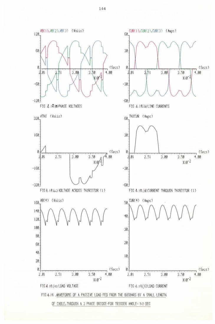
144
VB< 1 >, VB<2>,vB<3> <Volls) CUR< 1>,CUR<2>,CUR<3> <Amps) 1~ ~
+rrrt-.-,rr'T"T"n-.-.,...,...,--nr.,..,"'TT"T"n--.~+-r--r-Tih-1 < Secs ) ( Secs ) 4.00 4.00
- 120 -60 FIG 4 .I S (O) PHASE VOLT AGES FIG 4 - l~.lb)LINE CURRENTS
320 vTHY <Volts> 60 THYCUR <Amps)
160 30
'-h-r-+rr-TTT'TTT'T'"I"T'T'T"'"rT"T"I"T'T'T-,--r-T"T'T"T'T'"....,......._,., (Secs) 0--!-r-r-'h-rr-r-T"f"T'T'T'T"T"'T"',...,...,.,.-r--.-~TTT",.....,......,....,..~ (Secs ) 2.51 3 . 00 1 . 00 . 01 2 . 51 3 . 00 3 . 50 4 • 00
x10-2
- 160 -30
-320 -60 FIG~ \S{h)VOLTAGE ACROSS THYRISTOR (1) FIG 4 l'a£d)CURRENT THROUGH THYRISTOR ( 1)
160 VB< 4) (Volts) 50 CUR< 4 > (Amps)
140
120 40
100 30
80
60 20
40 10 '
20
0 (Secs) 0 2.01 2.51 3.00 3.50 4.00 2.01 2.51 3.00
x10-2
FIG+ l~(e) LOAO VOLTAGE FIG 4 l~{f)LOAO CURRENT
FIG4 - l~ .WAVEFORMS OF A PASSIVE LOAO FEO FROM THE BUSBARS BY A SMALL LENGTH
OF CABLE, THROUGH A 3 PHASE BRIDGE-FOR TRIGGER mGLE= ~o OEG
(Secs) 3.50 4.00
x10-2
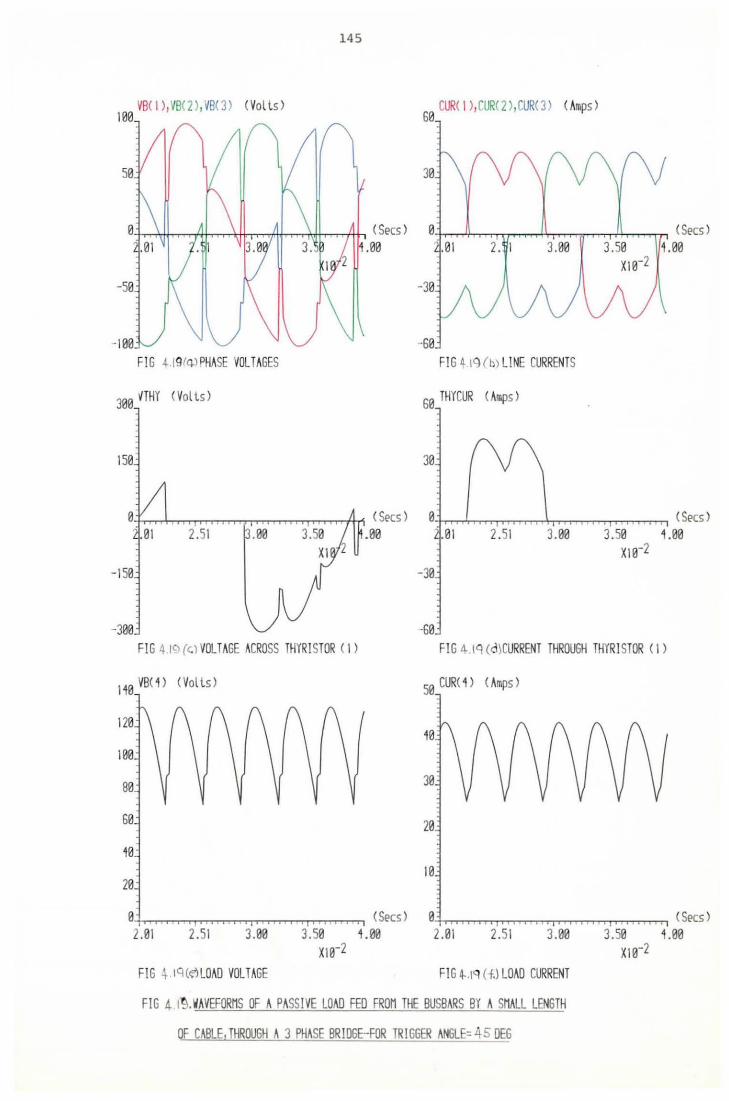
100 VB( 1 ) , VB< 2 ) , VB< 3 ) ( Vo lls )
50
145
CUR< 1 >,CUR< 2 >,CUR<3) (Amps> 60
30
+r-r-~"'T"!""T"+H-r"'T""r-Hir-r"'T""T'"T'l~..,...,....n,ft.,..-.....-+th (Secs ) +n-~,...,--.,..,.,...,..,...,..,.,-~-~r-r"T'T'T'rllT"'",...,....,+l-r...,........TT'l ( Secs ) 1.00 2. 1 3.00 3.50 1.00
x10-2
-50 -30
-100 -60 FIG 4.19fq.) PHASE VOLTAGES FIG 4.tq(b> LlNE CURRENTS
300 VTHY <Vol l s) 60 THYCUR <Amps>
150 30
+rr...,-+--rrr..,-,-rrrr-:rr..,.......,..-.-.......,.,.-T'T'T"T-.-++-n ( Secs ) 0-~-rr-r-T-"T""'T",...,...-,-,--r-+-r-T'"""T'"-...,.--,---rT'T-r-r-r-.,., ( Secs ) 2.51 .00 .01 2.51 3.00 3.50 1.00
x10-2
-150 -30
-300 -60 FIG 4 IC'l (<.) VOLTAGE ACROSS THYRI STOR ( 1) FIG a lG (d~CURRENT THROUGH THYRI STOR ( 1)
110 VB< 1 > (Volts) 50 CUR< 1 ) ( Amps >
120 10
100
80 30
60 20
10 10
20
0-t,--~..,.....,..T'T"T"''--.-,...--.,.,..,.....,..-r-r-rrr-r-...--r-r~ ( Secs ) 0-f-TT.,......,...."T"l"'T"rr-r-r--r--TTT'"""T'"-..,.....,..-r'T"T-r-r-r-'T"l (Secs ) 2.01 2.51 3.00 3.50 1.00 2.01 2.51 3.00 3.50 1.00
x1e-2 x1e-2
FIG 4- tq(~ LOAD VOLTAGE FIG 4- .t'-1 (f.) LOAD CURRENT
FIG 4 I .WAVEFORMS OF A PASSIVE LOAD FED FROM THE BUSBARS BY A SMALL LENGTH
OF CABLE, THROUGH A 3 PHASE BRIDGE-FOR TRIGGER ANGLE= 45 DEG
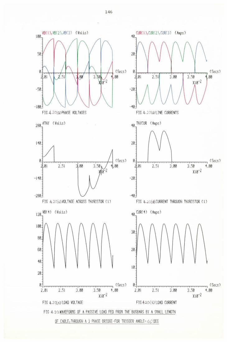
VB( 1 ),VB<2 >,VB(3) (Vol l s) 100
50
146
-1-r-r-~t-n-r~h-r--\-rrlrr"Mll,-,-f,,...,...,-n,......,_,-r-r+_.,., ( Secs ) .00
-50
- 100 FIG 4.]0(a> PHASE VOLTAGES
280 VTHY ( Volls >
110
CUR( 1 >,CUR( 2 >,CUR( 3) (Amps> 10
20
-f-r-r.,...,...,...,~T"""l'"'li'T""'"".,....,..,Jirrr-r.,..,...,.,~..,.,_,._~_,.., (Secs) 2.51 3. 00 .00
-20
-10 FIG 4 .20(0) LINE CURRENTS
10 THYCUR (Amps)
20
+rT.,...,...,...,n-r.-.,...,...,...,~,......,...,rT'T"'T"~_.,...,..T"T"T"''-rr+m ( Secs ) 0-f-r-r.,...,...,...,h--r"'f"T'T"1rr-r-.-rlfrr-r-,-,-,.--r-r.,...,...,....,...,......,.__,.., ( Secs ) 2.51 .00 1.00 .01 2.51 3. 00 3.50 1.00
x1e-2
-110 -20
-280 ·40 FIG 4.20(c.) VOLTAGE ACROSS THYRISTOR ( 1) FIG ~.2C{d~CURRENT THROUGH THYRISTOR ( 1 >
120 VB( 1 ) ( Vo lls >
40 CUR( 1 > ( Amps >
100 30
80
60 20
10 10
20
0-rr-r.,...,...,....,...,......,.TTT"r-T'"I"T"M"1r"T"T"'f'--r--l,..,...,r-r--r-r"'Tl ( Secs ) 0-~-r-r,_,.,c-r-TTTT"r-r-,-,-,rrr-r-,-,-,rTTT-n-r-r-T__,.., ( Secs ) 2.01 2.51 3.00 3.50 1.00 2.01 2.51 3. 00 3.50 4.00
x10-2 x1e-2
FIG 4 .20(e) LOAD VOLTAGE FIG 4lO(fJ LOAD CURRENT
FIG 4.20.WAVEFORMS OF A PASS IVE LOAD FED FROM THE'BUSBARS BY A SMALL LENGTH
OF CABLE,THROUGH A 3 PHASE BRIDGE-FOR TRIGGER ANGLE=.6;' DEG
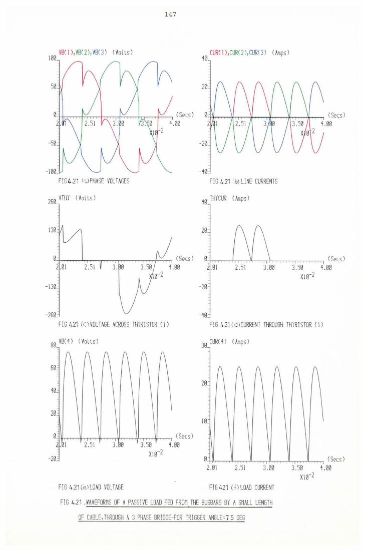
VB< 1 ) , VB< 2 ) , VB< 3 ) < Vo lls ) 100
50
147
0-H-r...--.--h,....,...:-+-..--,...,m-.--,....f-,-,-.,...,.......-r-:.,.--, < Secs ) 4.00
-50
·100 FIG 421 I·~) PHASE VOLT AGES
260 VTHY <Volls)
CUR< I >,CUR<2>,CUR<3> <Amps> 10
-++r,.......,.-...,.;r,-TT"T"'I-~~r----,--.~-:---.--.+r-r,...-,.-~~ (Secs) 4.00
-10 FIG 4.21 b) LI NE CURRENTS
40 THYCUR (Amps)
20
'-t-r--r-r-r-'--T...-.......r--,.,...-,----.-r--f--:---, <Secs) 0·-r.-...----:-'-...-_..._-r+--,.----,---..,.., (Secs) 2.51 3. 0 4 . 00 . 01 2 . 51 3 . 00 3 . 50 4 . 00
x1e-2 -130 -20
·260 ·40 FIG 4.21 (r:WOLTAGE ACROSS THYRISTOR < 1) FIG 4.21 <d>CURRENT THROUGH THYRISTOR < 1)
80 VB< 4 ) < Volls) 30 CUR( 4) <Amps)
60
40
20
0
-20
20
10
(Secs) . 1 2.51 3. 0 3.50 4.00
x1e-2 0 -++.-.,--,-.,..._,.,...,...,..,,......,_-r-r;r-m-.,...,........,~.,-,-,-..........,...,......, < Secs ) 2.01 2.51 3.00 3.50 4.00
x1e-2 FIG 4.21 (e) LOAD VOLTAGE FIG 4.21 ( f l LOAD CURRENT
FIG 4.21 .WAVEFORMS OF A PASS IVE LOAD FED FROM THE BUSBARS BY A SMALL LENGTH
OF CABLE, THROUGH A 3 PHASE BRIDGE-FOR TRIGGER ANGLE- 7 5 DEG
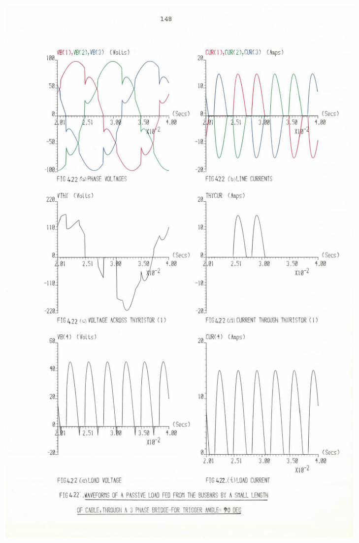
vB<l ) , VB< 2 ) , VB< 3 ) < Vo lls ) 100
50
148
CUR( 1 ) , fUR( 2 ) , CUR< 3) ( Amps ) 20
10
0 +r-r+-r-"'T"""""T~rr--,,.....,-,l:-:--:-"n-r+-:--,........,.tr"T'"T""rr-h-~. ( Secs ) 0-++r-+-n--rh-/r-n-,:-+.--J':--:-,r+-+--,-,rt-:-r.,.-,-+.-:r.-,-,. ( Secs ) 1.00 1.00
-50 -10
-100 -20_ F I G 422 re~) PHASE VOLT AGES FIG 1.12 ( b l L1 NE CURRENTS
220 VTHY ( Volls)
20 THYCUR ( Amps>
110 10
0;-.--r--___,.h--...,--~n-r--.-.---,-~h---, ( Secs ) 0--h-r-r-----'Y-T-_,_,.,r--r+--r--,--,--.,..,.--.--,-----, ( Secs ) 2.01 2.51 1.00 .• 01 2.51 3.00 3. 50 1.00
x10-2
-110 -10
·220 -20 FIG 4.22 (c.) VOLT AGE ACROSS THYR I STOR < 1 ) FIG4.22 t.dt CURRENT THROUGH THYRISTOR < 1)
60 VB(1) <Volls>
20
0--Hrr+-r-r~r-:-n--.-ir.-'.,.......,...,+-+---:~,...,...,.....fr.-'---, ( Secs ) 1.00
·20
FIG4.22 (e)LOAD VOLTAGE
20 CUR< 1 ) < Amps >
10
0 2.01
~ A
2.51
A
... 3.00
FIG 422.(f.)L0AD CURRENT
FIG 4.22 .. WAVEFORMS OF A PASSIVE LOAD FED FROM THE BUSBARS BY A SMALL LENGTH
OF CABLE, THROUGH A 3 PHASE BRIDGE-FOR TRIGGER ANGLE= 90 DEC
(\ A A
I
(Secs) . . 3.50 1.00
x10-2
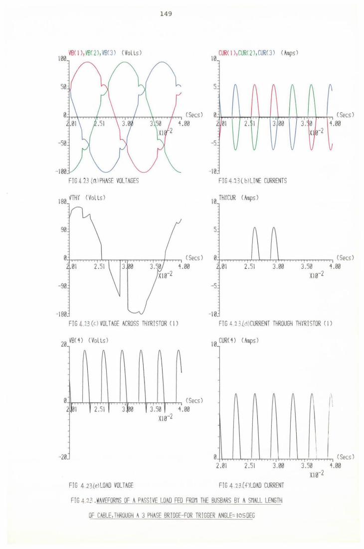
VB< 1 ) , VB< 2), VB< 3) ( Volls ) 100
50
0
-50
·100
FIG 423( a.\ PHASE VOLT AGES
180 VTHY <Volls)
90
149
(Secs) 4 . 00
CUR< 1 ) , CUR< 2 ) , CUR<3 ) ( Amps l 10
5
0
2 01 2. 1 3 00
-5
·10
FIG4.13(bl LINE CURRENTS
10 THYCUR < Amps )
5
r <Secs! 4.00
0-t-r-.-,.....,.....,...,...,..-.+-r.,..,......\'"TT"i,--,-,..,......,...,...,..,..,...,..f..,..,...,......, < Secs ) 0-~.,..,-,..,..,.....,.....,..n~-T+,...,..,r-'-r-r-~--r..,.....,.......,.....,......,......,r-r-"""'. ( Secs ) .01 2.51 4.00 .01 3.00 3.50 4.00
x10-2
-180 · 10
FIG .d.13 (c.l VOLTAGE ACROSS THYRISTOR < 1) FIG A. 13{-1lCURRENT THROUGH THYRISTOR < 1)
20 VB< 4) < Volls)
10 CUR( 4) (Amps )
A (\ (\ (\ (\ 1\
I
0 <Secs) d 01 2.51 3 ta0 3.50 4 .00
X10-2
-20
FIG 4 l3(e\LOAD VOLTAGE
0 2 .01
(\ (\
.. 2.51
(\
3.00
FIG 4. 23.( f \LOAD CURRENT
FIG 4 23 .WAVEFORMS OF A PA~SIVE LOAD FED FROM THE BUSBARS BY A SMALL LENGTH
OF CABLE, TH~OUGH..l] PHASE BRIDGE-FOR TRIGGER ANGLE= IOSDEG
{\
~\ /I
<Secs) 3.50 4.00
x10-2
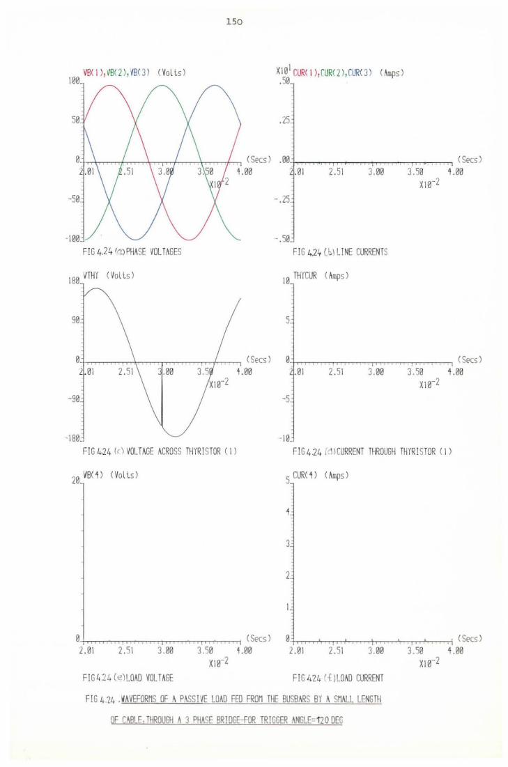
VB( I ), ~B<2> , ~B( 3) (Volts> le0
se
150
X I e I CUR< I ),lUR< 2) I CUR( 3) (Amps ) .se
.25
-t-r-r-\-r..,..-,frr--,---r-ltr'"""'""1rr-f--T.....--f---, < Secs ) . 00-t-r-T"'"T'"...--T"T""""""1.--....-,-,n-------:-T,.......,......,........,.-..,...,. ( Secs ) 4 . 00 . . 01 2. 5 I 3. 00 3. 50 4. 00
x1~r2 -50 -.25
-le0 -.50 FIG 4.24 1'1.1PHASE VOLT AGES FIG 424 (bl LINE CURRENTS
180 VTHY <Volls) 10 THYCUR ( Amps >
90 5
0-~-r---~>r-:-.,--,~.....,--,..--,-"T"'r'f...,....---, (Secs> e+r-,......,....-.,---:-.,---,n-----...-----. <Secs ) 2. 01 . 00 4. 00 2. 01 2. 51 3. 00 3. 50 4 . 00
xur2
-90 -5
-180 ·10_ FIG 424 fc) VOLTAGE ACROSS THYRISTOR <I > FIG 4 24 J 1 l CURRENT THROUGH THYR I STOR < I >
20 VB< 4 > < Vo lls > 5 CUR< 4 > < Amps >
3
2
0·-+r-...--.-:--.,..,.--..,....,...,..-,-....-----.-...,---..,...,-----t < Secs > e.-f-T-__,.......__,..,..............,_--+.....---'---.-.__._--n. < Secs > 2. 01 2. 51 3. 00 3 50 1. 00 2. 01 2. 51 3 00 3. 50 4 . 00
x10-2 x10-2
FIG 4.24 (")LOAD VOLT AGE FIG 4.24 'f l LOAD CURRENT
FIG 4.24 .WAVEFORMS OF A PASSIVE LOAD FED FROM THE BUSBARS BY A SMALL LENGTH
0~ C~BI F. THROUGH~ 3 PH~SE BRIDGE-FOR TRIGGER ANGLE-120DEC
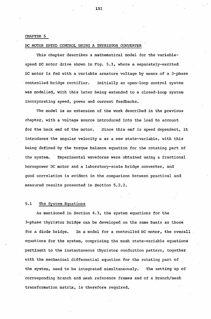
151
CHAPTER 5
DC MOTOR SPEED CONTROL USING A THYRISTOR CONVERTER
This chapter describes a mathematical model for the variable
speed DC motor drive shown in Fig. 5.1, where a separately-excited
DC motor is fed with a variable armature voltage by means of a 3-phase
controlled bridge rectifier. Initially an open-loop control system
was modelled, with this later being extended to a closed-loop system
incorporating speed, power and current feedbacks.
The model is an extension of the work described in the previous
chapter, with a voltage source introduced into the load to account
for the back emf of the motor. Since this emf is speed dependent, it
introduces the angular velocity w as a new state-variable, with this
being defined by the torque balance equation for the rotating part of
the system. Experimental waveforms were obtained using a fractional
horsepower DC motor and a laboratory-scale bridge converter, and
good correlation is evident in the comparison between practical and
measured results presented in Section 5.2.2.
5.1 The System Equations
As mentioned in Section 4.3, the system equations for the
3-phase thyristor bridge can be developed on the same basis as those
for a diode bridge. In a model for a controlled DC motor, the overall
equations for the system, comprising the mesh state-variable equations
pertinent to the instantaneous thyristor conduction pattern, together
with the mechanical differential equation for the rotating part of
the system, need to be integrated simultaneously. The setting up of
corresponding branch and mesh reference frames and of a branch/mesh
transformation matrix, is therefore required.
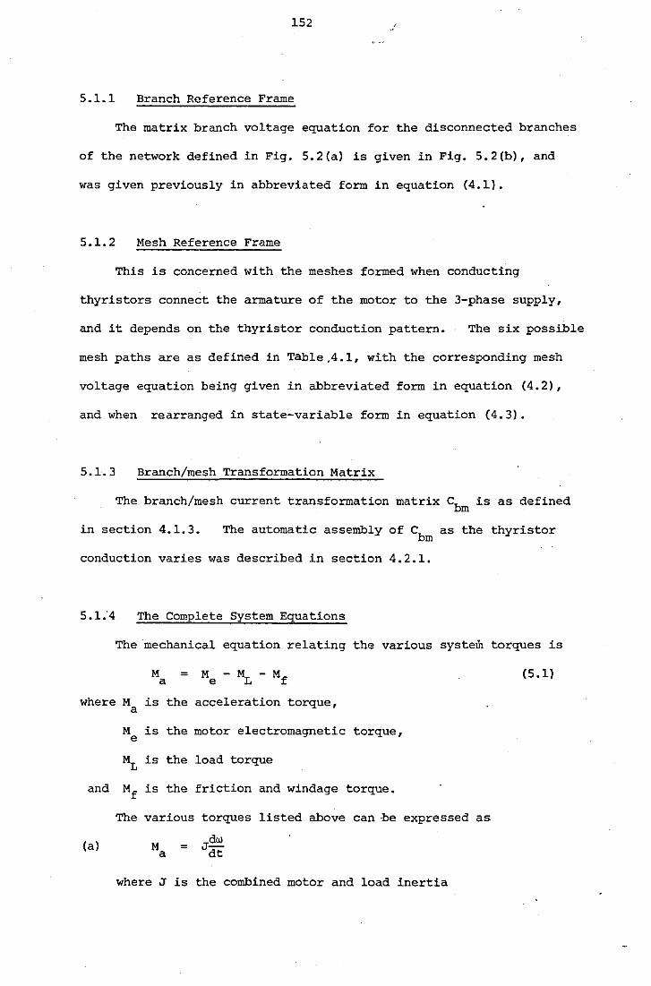
152
5.1.1 Branch Reference Frame
The matrix branch voltage equation for the disconnected branches
of the network defined in Fig. 5.2(a) is given in Fig. 5.2(b), and
was given previously in abbreviated form in equation (4.1).
5.1. 2 Mesh Reference Frame
This is concerned with the meshes formed when conducting
thyristors connect the armature of the motor to the 3-phase supply,
and it depends on the thyristor conduction pattern. The six possible
mesh paths are as defined in Table.4.1, with the corresponding mesh
voltage equation being given in abbreviated form in equation (4.2),
and when rearranged in state-variable form in equation (4.3).
5.1.3 Branch/mesh Transformation Matrix
The branch/mesh current transformation matrix Cbm is as defined
in section 4.1.3. The automatic assembly of cbm as the thyristor
conduction varies was described in section 4.2.1.
5.1.'4
where
and
(a)
The Complete System Equations
The mechanical equation relating the various system torques is
M = a
M is the a
M is the e
ML is the
Mf is the
The various
=
M -M -M e L f
acceleration torque,
motor electromagnetic torque,
load torque
friction and windage torque.
torques
Jdw dt
listed above can be expressed
where J is the combined motor and load inertia
(5 .1)
as
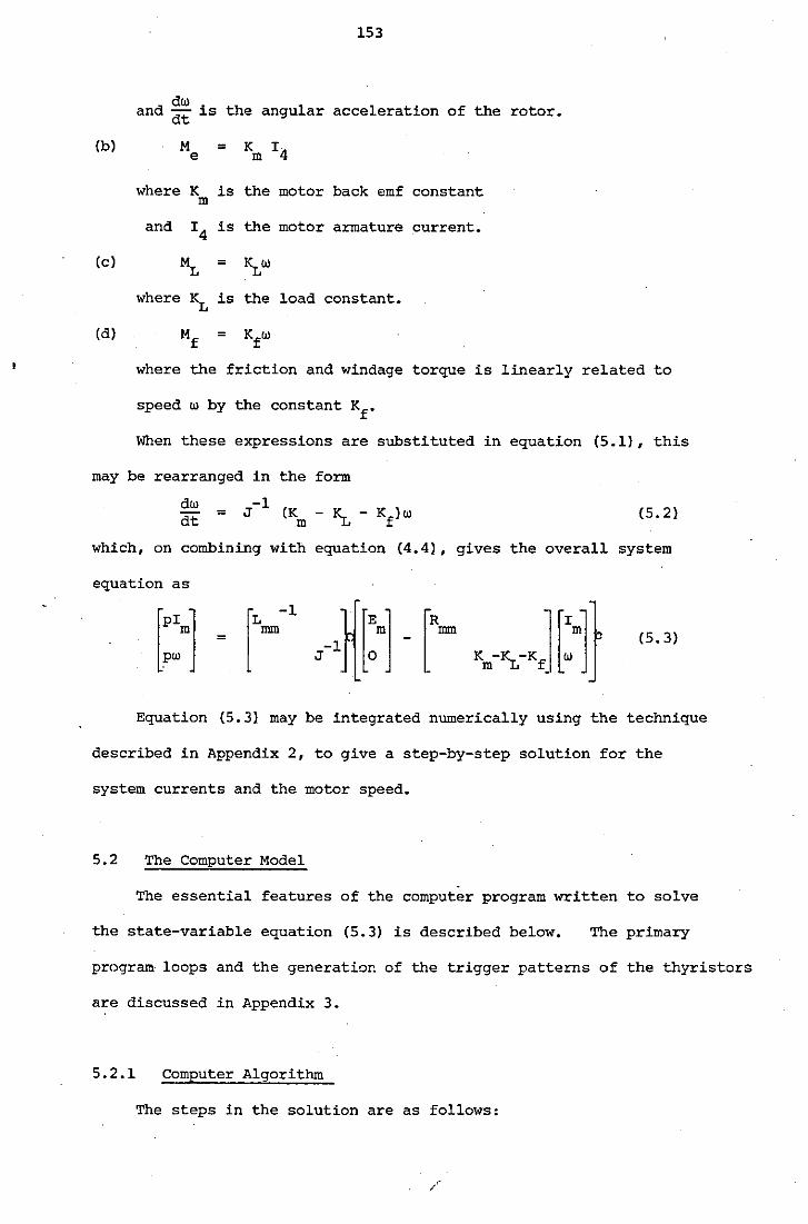
{b)
{c)
{d)
153
dw and dt is the angular acceleration of the rotor.
where
and
M e
K m
I4
ML
where ~
Mf
=
is
is
=
is
=
the motor back emf constant
the motor armature current.
~"' the load constant.
Kfw
where the friction and windage torque is linearly related to
speed w by the constant Kf.
When these expressions are substituted in equation {5.1), this
may be rearranged in the form
dw dt = (5.2}
which, on combining with equation (4.41, gives the overall system
equation as
(5. 3)
Equation (5.3) may be integrated numerically using the technique
described in Appendix 2, to give a step-by-step solution for the
system currents and the motor speed.
5.2 The Computer Model
The essential features of the computer program written to solve
the state-variable equation {5.3) is described below. The primary
program· loops and the generation of the trigger patterns of the thyristors
are discussed in Appendix 3.
5.2.1 Computer Algorithm
The steps in the solution are as follows:
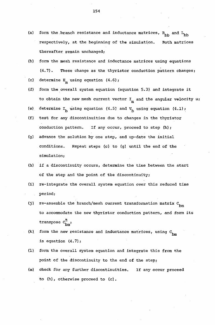
154
(a) form the.branch resistance and inductance matrices, ~band ~b
respectively, at the beginning of the simulation. Both matrices
thereafter remain unchanged;
(b) form the mesh resistance and inductance matrices using equations
(c)
(d)
(4. 7). These change as the thyristor conduction pattern changes;
determine E using equation (4.6); m
form the.overall system equation (equation 5.3! and integrate it
to obtain the new mesh current vector I and the angular velocity w; m
(e) determine Ib using equation (4.5! and Vb using equation (4.1);
(f) test for any discontinuities due to changes in the thyristor
conduction pattern. If any occur, proceed to step (h) ;
(g) advance the solution by one step, and up-date the initial
conditions. Repeat steps (cl to (gl until the end of the
simulation;
(h) if a discontinuity occurs, determine the time between the start
of the step and the point of the discontinuity;
(il re-integrate the overall system equation over this reduced time
period;
(jl re-assemble the branch/mesh current transformation matrix Cbm
to accommodate the new thyristor conduction pattern, and form its
transpose c~m'
(kl form the new resistance and inductance matrices, using Cbm
in equation (4.7);
(1) form the overall system equation and integrate this from the
point of the discontinuity to the end of the step;
(ml check for any further discontinuities. If any occur proceed
to (h), otherwise proceed to (cl.
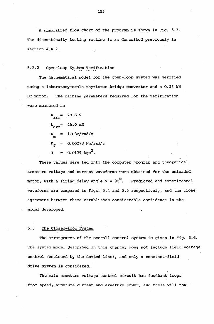
155
A simplified flow chart of the program is shown in Fig. 5.3.
The discontinuity testing routine is as described previously in
section 4.4.2.
5.2.2 Open-loop System Verification
The mathematical model for the open-loop system was verified
using a laboratory-scale thyristor bridge converter and a 0.25 kW
DC motor. The machine parameters required for the verification
were measured as
R = 2o.6 n arm
L = 46.0 mH arm
K m =
=
=
l.OSV/rad/s
0.00278 Nm/rad/s
0.0139 kgm2
These values were fed into the computer program and theoretical
armature voltage and current waveforms were obtained for the unloaded
0 motor, with a firing delay angle a = 90 • Predicted and experimental
waveforms are compared in Figs. 5.4 and 5.5 respectively, and the close
agreement between these establishes considerable confidence in the
model developed.
5.3 The Closed-loop System
The arrangement of the overall control system is given in Fig. 5.6.
The system model described in this chapter does not include field voltage
control (enclosed by the dotted line), and only a constant-field
drive system is considered.
The main armature voltage control circuit has feedback loops
from speed, armature current and armature power, and these will now
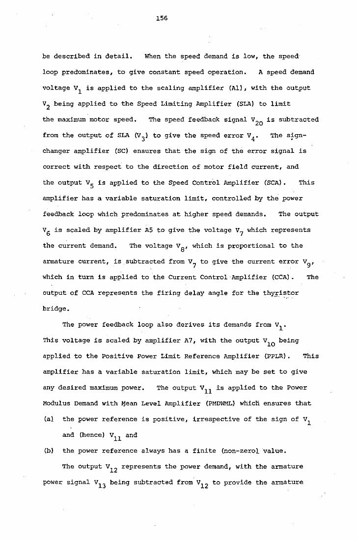
1S6
be described in detail. When the speed demand is low, the speed
loop predominates, to give constant speed operation. A speed demand
voltage v1
is applied to the scaling amplifier (All, with the output
v2 being applied to the Speed Limiting Amplifier (SLAJ to limit
the maximum motor speed. The speed feedback signal v20
is subtracted
from the output of SLA (v3
J to give the speed error v4
• The s~gn-
changer amplifier (SCJ ensures that the sign of the error signal is
correct with respect to the direction of motor field current, and
the output VS is applied to the Speed Control Amplifier (SCAJ. This
amplifier has a variable saturation limit, controlled by the power
feedback loop which predominates at higher speed demands. The output
v6 is scaled by amplifier AS to give the voltage v7
which represents
the current demand. The voltage v8
, which is proportional to the
armature current, is subtracted from v7
to give the current error v9
,
which in turn is applied to the Current Control·Amplifier (CCAJ. The
output of CCA represents the firing delay angle for the thyristor ~·· ..
bridge.
The power feedback loop also derives its demands from v1
•
This voltage is scaled by amplifier A7, with the output v10
being
applied to the Positive Power Limit Reference Amplifier (PPLRJ. This
amplifier has a variable saturation limit, which may be set to give
any desired maximum power. The output v11
is applied to the Power
Modulus Demand with ~ean Level Amplifier (PMDWMLJ whicli ensures that
(aJ the power reference is positive, irrespective of the sign of v1
and (hence) v11 and
(bl the power reference always has a finite (non-zeroL value.
The output v12
represents the power demand, with the armature
power signal v13 being subtracted from v12
to provide the armature
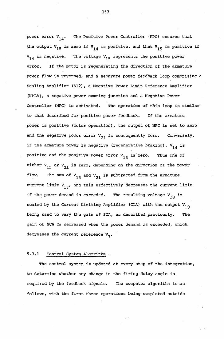
157
power error v14 • The Positive Power Controller (PPC) ensures that
the output v15 is zero if v14 is positive, and that v15 is positive if
v14 is negative. The voltage v15 represents the positive power
error. If the motor is regenerating the direction of the armature
power flow is reversed, and a separate power feedback loop comprising a
Scaling Amplifier (Al2), a Negative Power Limit Reference Amplifier
(NPLAl, a negative power summing junction and a Negative Power
Controller (NPC) is activated. The operation of this loop is similar
to that described for positive power feedback. If the armature
power is positive (motor operation), the output of NPC is set to zero
and the negative power error v21
is consequently zero. Conversely,
if the armature power is negative (regenerative braking], v14
is
positive and the positive power error v15
is zero. Thus one of
either v15 or v21 is zero, depending on the direction of the power
flow. The sum of v15
and v21 is subtracted from the armature
current limit v17 , and this effectively decreases the current limit
if the power demand is exceeded. The resulting voltage v18 is
scaled by the Current Limiting Amplifier (CLAl with the output v19
being used to vary the gain of SCA, as described previously. The
gain of SCA is decreased when the power demand is exceeded, which
decreases the current reference v7
•
5.3.1 Control System Algorithm
The control system is updated at every step of the integration,
to determine whether any change in the firing delay angle is
required by the feedback signals. The computer algorithm is as
follows, with the first three operations being completed outside
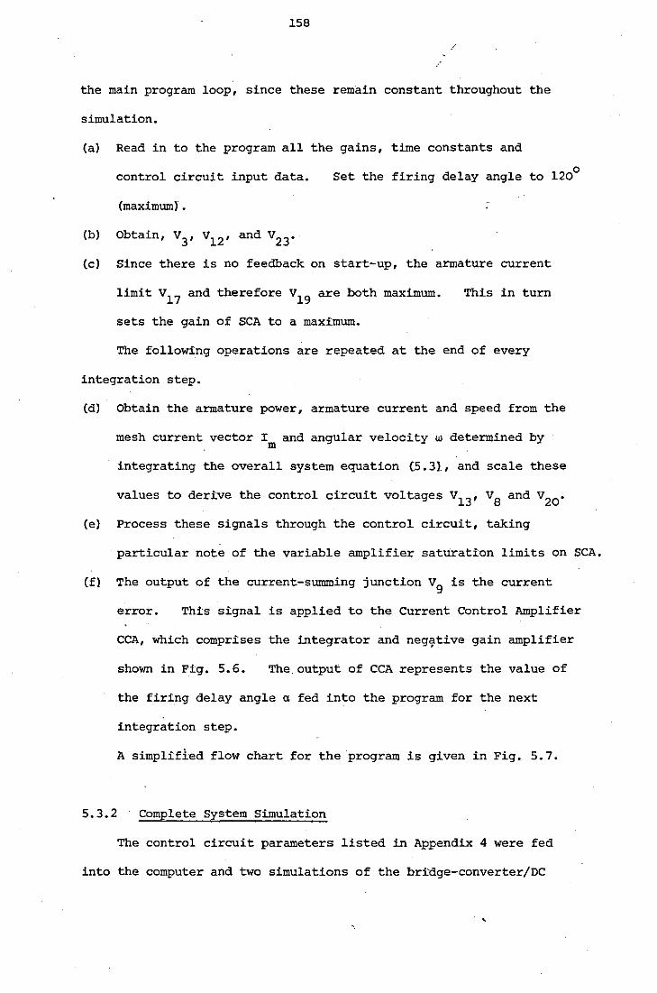
158
/
the main program loop, since these rem·ain constant throughout the
simulation.
(a) Read in to the program all the gains, time constants and
control circuit input data. Set the firing delay angle to 120°
(maximum)'.
(b) Obtain, v3
, v12 , and v23 •
(c) Since there is no feedback on start-up, the armature current
limit v17
and therefore v19
are both maximum. This in turn
sets the gain of SCA to a maximum.
The following operations are repeated at the end of every
integration step.
(d) Obtain the armature power, armature current and speed from the
mesh current vector I and angular velocity w determined by m
integrating the overall system equation (5.31, and scale these
values to derive the control circuit voltages v13 , v8 and v20 •
(e) Process these signals through the control circuit, taking
particular note of the variable amplifier saturation limits on SCA.
(fl The output of the current-summing junction v9
is the current
error. This signal is applied to the Current Control Amplifier
CCA, which comprises the integrator and neg~tive gain amplifier
shown in Fig. 5.6. The. output of CCA represents the value of
the firing delay angle a fed into the program for the next
integration step.
A simplified flow chart for the program is given in Fig. 5. 7.
5.3.2 Complete System Simulation
The control circuit parameters listed in Appendix 4 were fed
into the computer and two simulations of the britlge-converter/DC
'
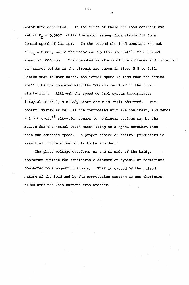
159
motor were conducted. In the first of these the load constant was
set at~= 0.0637, while the motor ran-up from standstill to a
demand speed of 200 rpm. In the second the load constant was set
at ~ = 0.008, while the motor ran-up from standstill to a demand
speed of 1000 rpm. The computed waveforms of the voltages and currents
at various points in the circuit are shown in Figs. 5.8 to 5.11.
Notice that in both cases, the actual speed is less than the demand
speed (164 rpm compared with the 200 rpm required in the first
simulation}. Although the speed control system incorporates
integral control, a steady-state error is still observed. The
control system as well as the controlled unit are nonlinear, and hence
a limit cycle21
situation common to nonlinear systems may be the
reason for the actual speed stabilising at a speed somewhat less
than the demanded speed. A proper choice of control parameters is
essential if the situation is to be avoided. ·
The phase voltage waveforms on the AC side of the bridge
converter exhibit the considerable distortion typical of rectifiers
connected to a non-stiff supply. This is caused by the pulsed
nature of the load and by the commutation process as one thyristor
takes over the load current from another.
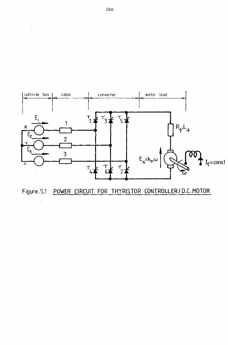
160
infint te bus cable r~nverte.':_ __ r~
E, T1 T3 Ts 1
R Rt,L4 Ez
2 '(
E3 3
C.okmw I I'.
\ T T 6 2
Figure. 5.1 POWER CIRCUIT FOR THYRIS TOR CONTROLLER I D.C. MOTOR

161
E, .. z, I,
• 0 . I • • 14
~ Ez v, ... Ze. l.z
0 • ~ • z"- v~,. ~
E3 ".! ...
0 z3 13 E~,.+ • .... •
... v3
Figure. 5.2 (a). BRANCH REFERENCE FRAME.
A
E1
sin w5 t + vl ~+pLl 0 0 0 Il A 211 E1
sin (wst - 3) + v2 R2+pL2 0 0 I2 A 211 = E1 sin (w5 t +3> + v3 SYMMETRICAL R3+pL3 0 I3
ABOUT
K w + v4 LEADING
m DIAGONAL R4+pL4 I4
= Supply angular frequency
w = Rotor angular velocity
Figure.S:2 . (bl. MATRIX BRANCH VOLTAGE EQUATION.
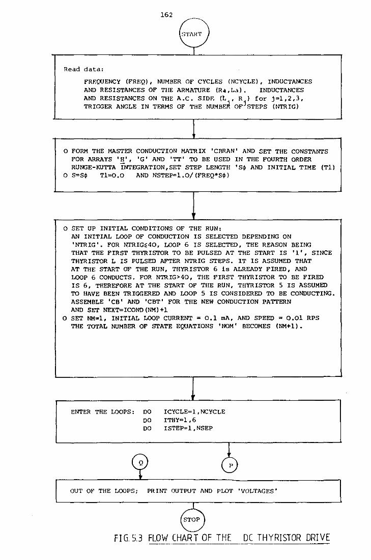
162
e Read data:
FREOOENC'i (FREQ) , NUMBER OF CYCLES (NCYCLE) , INDUCTANCES AND RESISTANCES OF THE ARMATURE (R.,L,>), INDUCTANCES AND RESISTANCES ON THE A,C, SIDE (t , R ) for j=l,2,3, TRir~ER ANGLE IN TERMS OF THE NUMBE~ OFjSTEPS (NTRIG)
0 FORM THE MASTER CONDUCTION MATRIX 'C!lRAN' AND SET TilE CONSTANTS FOR ARRA YS '!!_' , 'G' AND 'TT' TO BE USED IN TilE FOURTII ORDER RUNGE-KUTTA INTEGRATION,SET STEP LENGTH 'S$ AND INITIAL TIME (Tl)
0 S=S$ Tl=O.O AND NSTEP=l.O/(FREQ*S$)
0 SET UP INITIAL CONDITIONS OF THE RUN: AN INITIAL LOOP OF CONDUCTION IS SELECTED DEPENDING ON 'NTRIG'. FOR NTRIG~40, LOOP 6 IS SELECTED, THE REASON BEING THAT THE FIRST THYRISTOR TO BE PULSED AT THE START IS '1', SINCE THYRISTOR L IS PULSED AFTER NTRIG STEPS. IT IS ASSUMED THAT AT THE START OF THE RUN, THYRISTOR 6 is ALREADY FIRED, AND LOOP 6 CONDUCTS. FOR NTRIG>40, THE FIRST TIIYRISTOR TO BE FIRED IS 6, THEREFORE AT THE START OF THE RUN, THYRISTOR 5 IS ASSUMED TO HAVE BEEN TRIGGERED AND LOOP 5 IS CONSIDERED TO BE CONDUCTING. ASSEMBLE 'CB' AND 'CBT' FOR THE NEW CONDUCTION PATTERN AND SET NEXT=ICOND(NM)+l
0 SET NM=l, INITIAL LOOP CURRENT = 0,1 mA, AND SPEED = 0,01 RPS THE TOTAL NUMBER OF STATE EOOATIONS 'NOM' BECOMES (NM+l) •
ENTER THE LOOPS: DO ICYCLE=l, NCYCLE DO ITH'i=l,6 DO ISTEP=1,NSEP
Q cb OUT Qlo' THE LOOPS; PRINT OUTPUT AND PLOT 'VOLTAGF.S'
F!G.5.3 FLOW CHART OF THE DC THYRJSTOR DRIVE
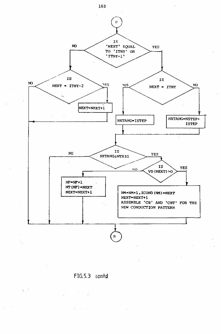
NO
NO
IS
NEXT = ITHY-2
163
IS 'NEXT'
TO 'ITHY' 'ITHY-1'
YES
IS
NEXT • ITHY
NEXT= NEXT+ 1
NO IS
NXTANG=NSTEP+ I STEP
NXTANG>NTRIG ~
NF=NF+l NT(NF)•NEXT
NEXT=NEXT+l
FIG.5.3 contd
----NO
NM=NM+l, ICOND (lfl) •NEXT NEXT= NEXT+ 1
YES
ASSEMBLE 'CB' AND 'CBT' FOR THE NEW CONDUCTION PATTERN
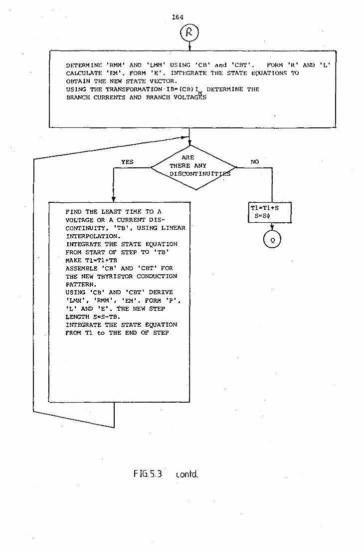
164
Dl-7I'ERMINE 'RMM' AND 'LMM' USING 'CB' and 'CBT'. l'"'ORM 'H' AND *L' CALCULATE 'EM'. FORM 'F;'. IN"n:GRATF; 1'11E STATE E(XJATIONS 1'0 OBTAIN THE NEW STATE VECTOR. USING THE TRANSFORMATION· IB= (CB) I DETERMINE THE BRANCH CURRENTS AND BRANCH VOL TAG~S
YES
FIND THE LEAST TIME TO A VOLTAGE OR A CURRENT DISCOill'INUITY, 'TB', USING LINEAR INTERPOLATION. INTEGRATE THE STATE EQUATION FROM START OF STEP TO 'TB' MAKE Tl=Tl+TB ASSEMBLE 'CB' AND 'CBT' FOR THE NEW THYRISTOR CONDUCTION PATTERN. USING 'CB' AND 'CBT' DERIVE 'LMU', 'RMM', 'EM'. FORM 'P' I
'L' AND 'E'. THE NEW STEP LENGTH S=S-TB. INTEGRATE THE STATE EQUATION FROM Tl to THE END OF STEP
FIG.S. 3 LOnrd.
NO
Tl=Tl+S S=S~
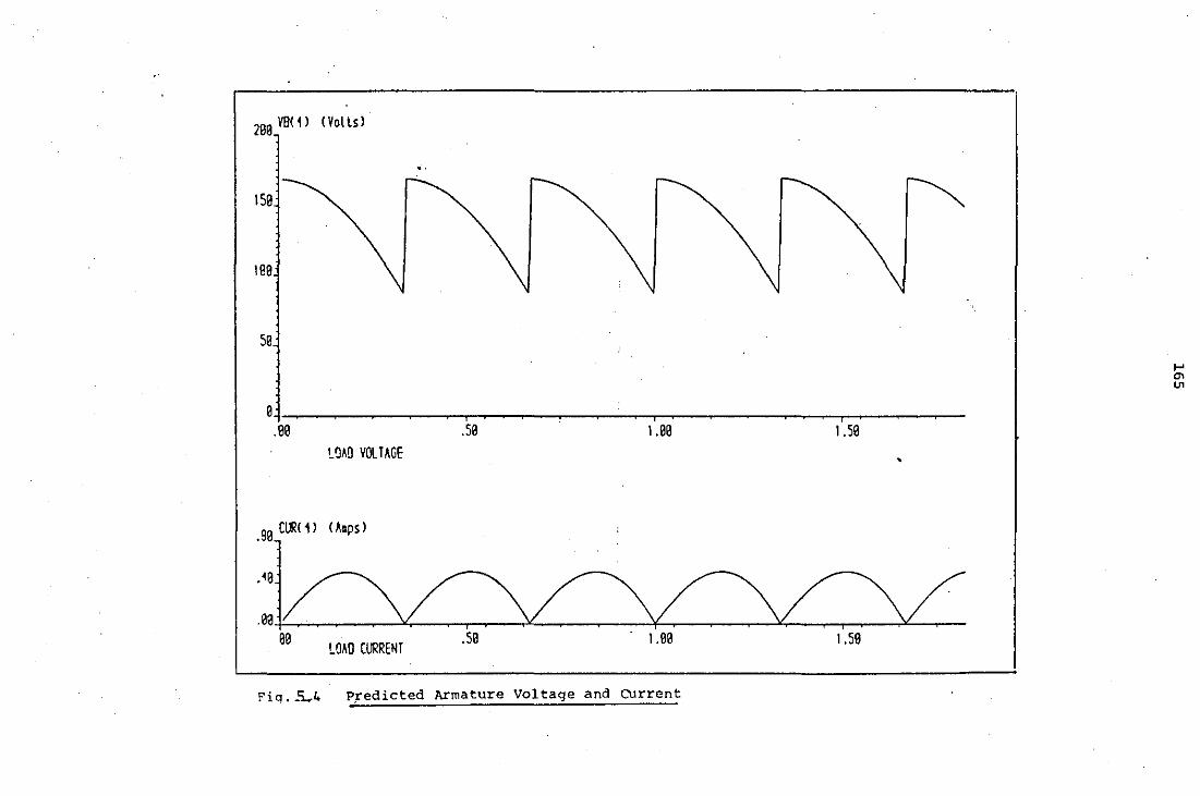
299 VB< 1) (Volts l
150
109
se
LOAO VOLT AGE
.99 (lJR( 1) < A•ps l
. ~a
.ea ea
LOAD CURRENT .se l.e9
F'iq. _'i.-4 P,redicted Armature Voltage and Olrrent
'
1.59
1-'
"' U1
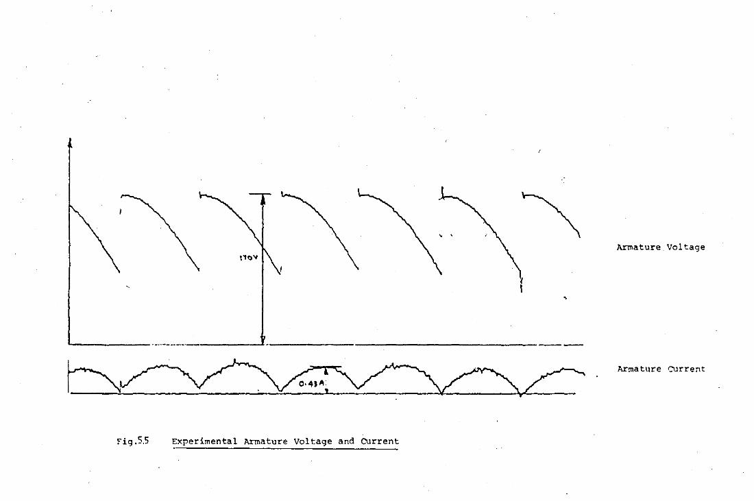
Armature Voltage
Armature OJrrent
Fig .5.5 Experimental Armature Voltage and CUrrent
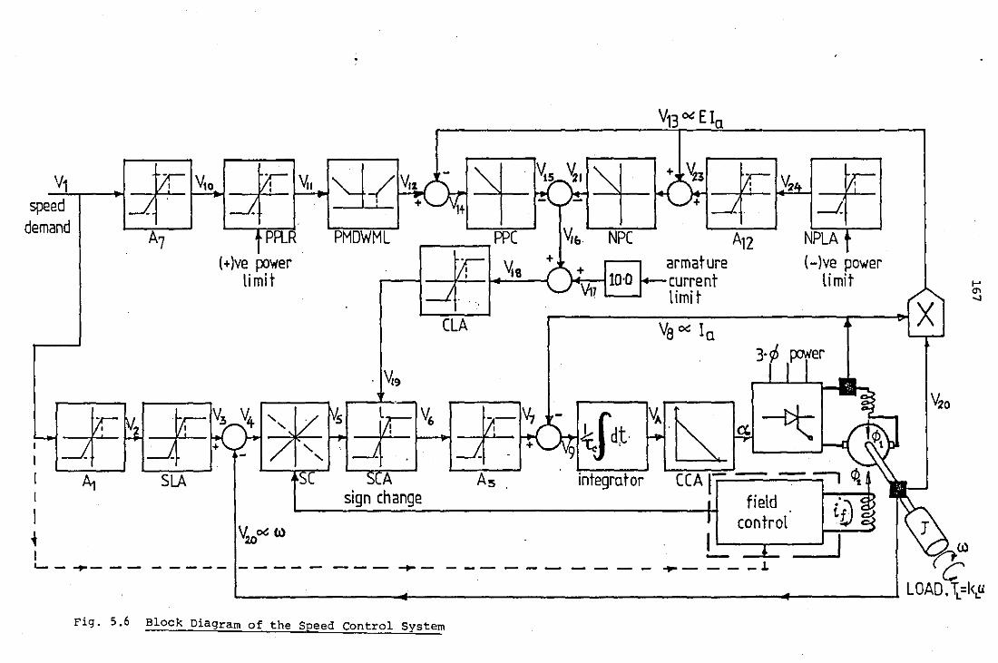
'11 . speed
demand
W I Y1o. Vr V.. IJ. 1_).
A7 .....__......,t P=-:!R.J
(+)ve p:~wer limit
PMuWML ,.--...,..-_,, PPC
.---l=f= ~. CLA
V,& NPC A12 + + armature
"\ .\11, 10·0 f--current
NPLAt (-)ve power
limit "' limit
~------------------~----~vX Ya o.: la
.v,9
3·r,1er
~. ~~ =f· . v3~4 ',I/ ~s =fL 1 v6 )=· jY1 l- ~., r- I~·~ In: -et -~~ ,4 ~ 1::<../ / ' f-f' ~ ~ le dt ~ r: ,~t ~ , - ~- , - . . - I +'\,/vs , I ~ SLA FSC . --sLA A5 . .,_ln.,.-teg-ra-,..to_....r CCA 1 - ::;-, ~ 1 s1gn change • field ~'D ~ I I •f c
V. con trot . c:
1 2/Jo.: (I) I 1 I - ' ,(1)
'-- ~--- ----- ----- --- ~- --- --- - - - - ~- -- - J. ( ;-.
~----------~----------------------------.-------~LOAD~cl<~ Fig. 5.6 Block Diagram of the Speed Control System
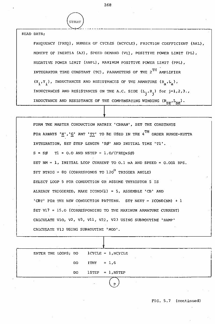
168
,---------------_8. ----------------------·-·-----------., READ DATA;
FREQUENCY (FREQ), NUMBER OF CYCLES (NCYCLE), FRICTION COEFFICIENT (AKL),
l·lOHC~!T OF INERTIA (A,J), SPEF.D DEMAND (Vl), POSITIVE POWF.R LIMIT (PL),
NEGA1'IVE POWER LIMIT (ANPL), MAXIMUM POSITIVE POWER LIMIT (PPL),
INTEGRATOR TIME CONSTANT (TC), PARAMETERS OF THE 2TH AMPLIFIER
(X.,Y.), INDUCTANCES AND RESISTANCES OF THE ARMATURE (R ,L ), 1 1 a a
INDUCTANCES AND RESISTANCES ON THE A.C. SIDE (L.,R.) for j=1,2,3., J J
INDUCTANCE AND RESISTANCE OF THE COMPENSATING WINDING (RSE'LSE).
FORM THE MASTER CONDUCTION MATRIX 'CBRAN', SET THE CONSTANTS
FOR ARRAYS '~','£' ANT 'TT' TO BE USED IN THE 4TH ORDER RUNGE-KUTTA
INTEGRATION, SET STEP LENGTH 'S~' AND INITIAL TIME 'T1'.
S = S!1l T1 = 0.0 AND NSTEP = 1.0/(FREQxS!Il)
SET NM = 1, INITIAL LOOP CURRENT TO 0.1 mA AND SPEED= 0.001 RPS.
SET NTRIG = 80 (CORRESPONDS TO 120° TRIGGER ANGLE)
SELECT LOOP 5 FOR CONDUCTION OR ASSUME THYRISTOR 5 IS
ALREADY TRIGGERED, MAKE ICOND(1) = 5, ASSEMBLE 'CB' AND
'CBT' FOR THE NEW CONDUCTION PATTERN. SET NEXT = ICOND(NM) + 1
SET V17 = 15.0 (CORRESPONDING TO THE MAXIMUM ARMATURE CURRENT)
CALCULATE VlO, V2, V3, Vll, V?.2, V23 USING SUBROUTINE 'RAMP'
CALCULATE V12 USING SUBROUTINE 'MOD'.
ENTER THE LOOPS; DO 1CYCLE = 1 ,NCYCLE
DO ITIIY = 1,6
DO 1STEP = 1, NSTEP
G) FIG. 5. 7 (continued)
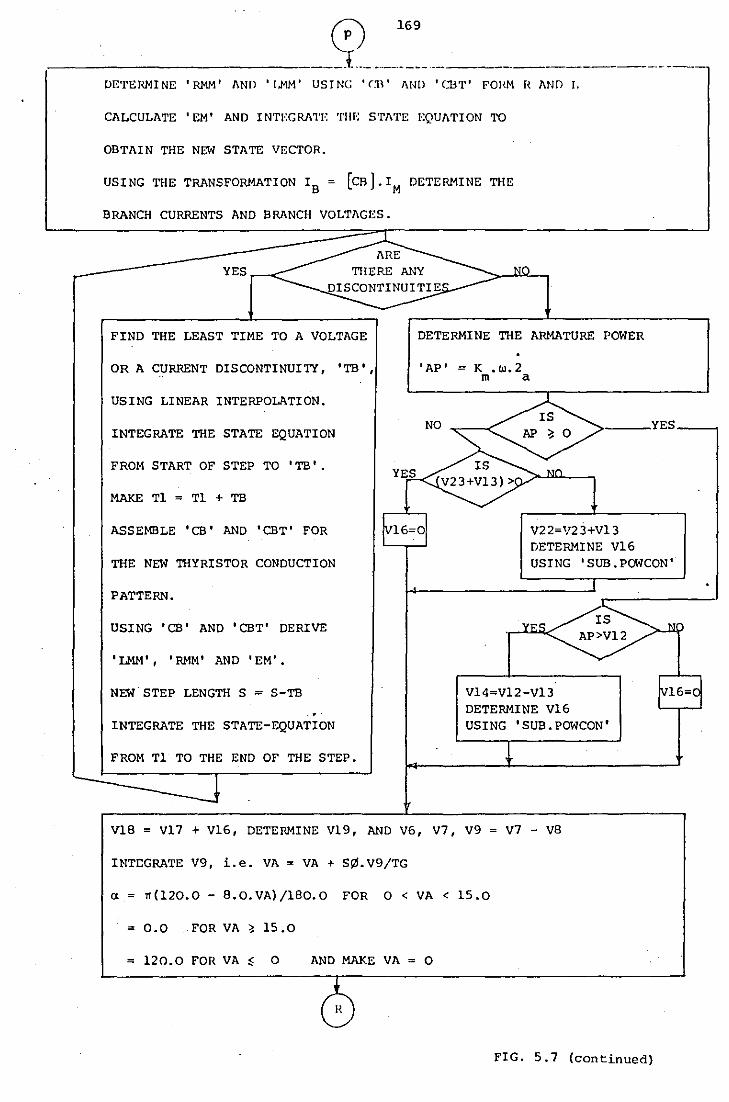
169 0 .---------------1·--------------------------------
DETERMINE 'RMM' 1\ND '!.MM' USING '(1~' 1\ND 'CBT' FOHM H 1\ND I.
CALCULATE 'EM' AND INTEGRATE TilE STIITE EQUATION TO
OBTAIN THE NEW STIITE VECTOR.
USING THE TRANSFORMATION IB = [CB). IM DETERMINE THE
BRANCH CURRENTS AND BRANCH VOLTIIGES.
FIND THE LEAST TIME TO A VOLTAGE
OR A CURRENT DISCONTINUITY, 'TB' ,
USING LINEAR INTERPOLATION.
INTEGRATE THE STATE EQUATION
FROM START OF STEP TO 'TB'.
MAKE Tl = Tl + TB
ASSEMBLE 'CB' AND 'CBT' FOR
THE NEW THYRISTOR CONDUCTION
PATTERN.
USING 'CB' AND 'CBT' DERIVE
• LMM', I RMM' AND I EM'.
NEW STEP LENGTH S = S-TB
INTEGRATE THE STATE-EQUATION
FROM Tl TO THE END OF THE STEP.
DETERMINE THE ARMATURE POWER
'AP' ::::: K .w.2 m a
>----YES _ ___,
V22=V23+V13 DETERMINE Vl6 USING 'SUB.POWCON'
V14=V12-Vl3 DETERMINE Vl6 USING 'SUB.POWCON'
V18 = V17 + Vl6, DETERMINE V19, AND V6, V7, V9 V7 - VB
INTEGRATE V9, i.e. VII = VII + S(l!_ V9/TG
a= n(l20.0- B.O.VII)/180.0 FOR 0 <VII< 15.0
= 0.0 FOR VI\ 3 15.0
= 120.0 FOR VII ~ 0 AND MAKE V 1\ 0
FIG. 5.7 (continued)
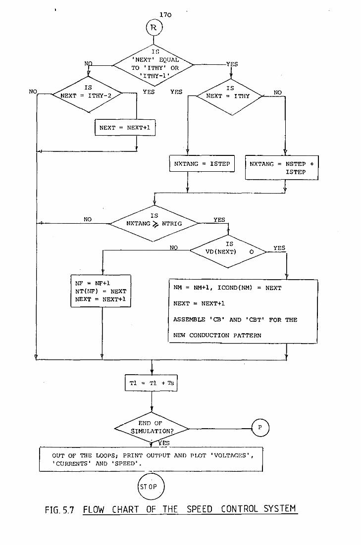
NO
NO
NF = NF+l NT(!lF) = NEXT NEXT = NEXT+!
170
'NEXT' EQUAL TO 'ITHY'
'ITHY-1'
YES
OR YES
YES NEXT = ITHY
NXTANG = ISTEP
N
NO
NXTANG = NSTEP + I STEP
YES
NM = NM+l, ICOND(NM) NEXT
NEXT = NEXT+!
ASSEMBLE 'CB' AND 'CBT' FOR THE
NEW CONDUCTION PATTERN
OUT OF THE LOOPS; PRINT OUTPUT ANn PLOT 'VOLTAGES', 'CURRENTS' AND 'SPEED'.
8 FIG. 5.7 FLOW CHART OF THE SPEED CONTROL SYSTEM
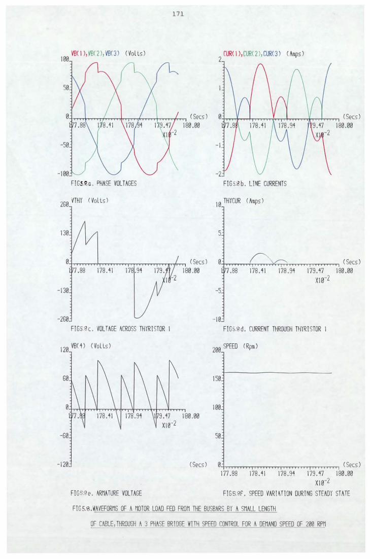
100 VB< 1 ), VB<2>, VB<3> <Volls)
50
0
-50
-100 FIGs ~ a . PHASE VOLTAGES
260 ~THY <Volls)
130
0 7.88 178. 41
-130
-260 FIGS'ac. VOLTAGE ACROSS THYRISTOR 1
120 V8(4) <Volls)
-60
-120
FIGS.tt!e. ARMATURE VOLTAGE
171
(Secs) 180.00
\
(Secs) 180.00
CUR( 1 ) , CUR( 2 ) , CUR< 3) ( A 'lips ) 2
0
-1
-2 FI GSS b. LINE CURRENTS
10 THYCUR < Arnps)
5
0 r 7.88 178.41 178 .94
-5
-10
179.47 X10⁻²
F I GS.<a d. CURRENT THROUGH THYR I STOR 1
200 SPEED <Rpm)
150
100
50
(Secs) 180.00
<Secs) 180.00
( Secs ) 0 ( Secs ) 177.88 178.41 178 .94 179. 47 180.00
x10-2 Fl G S.~lF . SPEED VARIATION DURING STEADY STATE
FIGS.e .WAVEFORMS OF A MOTOR LOAD FED FROM THE BUSBARS BY A SMALL LENGTH
~r CABLE,THROUGH A 3 PHA~E BRIDGE WITH SPEED fONTROL FOR A DEMAND SPEED OF 200 RPM
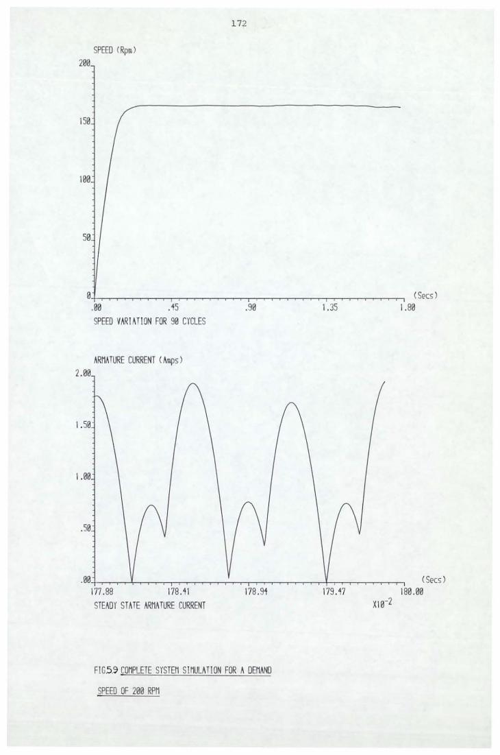
172
SPEED <Rpm> 200
150
100
50
0-t-r"""'T'"'"""r--..-...--.-...,.--,--r-y--r-,.....,-....--.-"""T'"'""T--..-T'"""T"""___,...--.--.--r-...--.-...,.--,---,--,-.-..---..-.,..-,--.--.~ < S~:>cs ) .00 . 45 .90 1.35 1 .80 SPEED VA~IATION FOR 90 CYCLES
ARMATURE CURRENT <Amps) 2.00
1.50
1.00
.50
. 00+-,----r-~~~,-r-.,..-,----r-~-.-...--.-....-,-"""T'"'""T--.--...--.-...,.--,-.....---.-.-...--.-............. -+-->-.-,.-,-.....-.--.--.-.-. < S~:>cs >
177.88 178.41 178.94 179.47 180.00 STEADY STATE ARMATURE CURRENT
FIG.5.9 COMPLETE SYSTEM SIMULATION FOR A DEMAND
SPEED OF 200 RPM
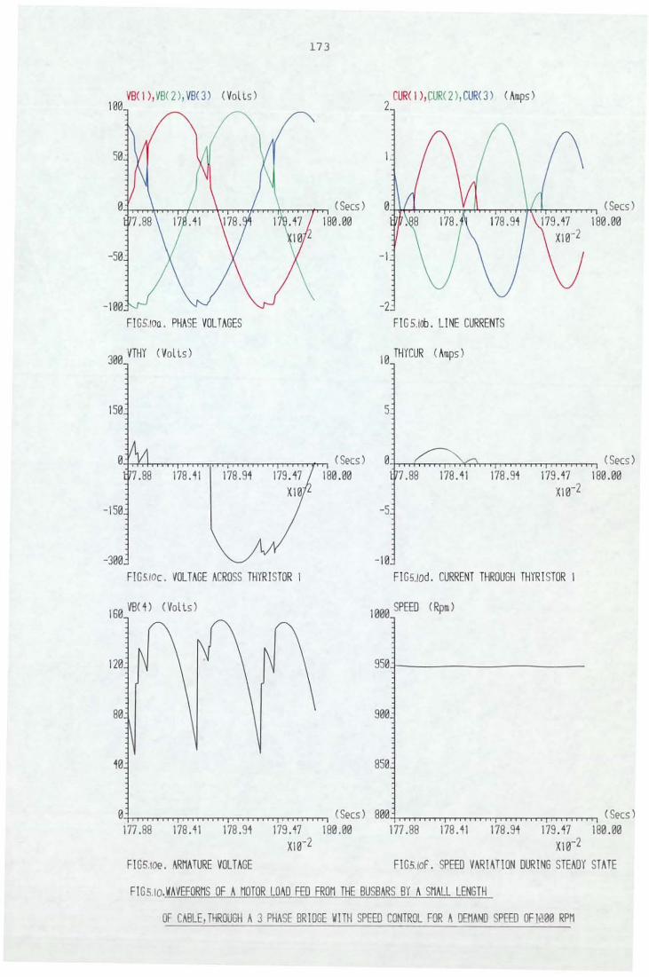
173
100 VB< 1), VB< 2 >, VB<3 > <Volts>
2 CUR( I >,CUR<2>,CUR(3) <Amps>
50
0-+-r-r...-Mn"T"T"T"T'T"'h...,...,...,..-n-.-,...,...,...,..Tfrr,"T"T""iiT'"T"T'""...,.......,....., ( Secs ) 0-H+...+n...,...,...,..T"T"n~~,-,-,-rTTT~h-fl-r"T'T'T'"I"TT"T"T'T'1 < Secs ) 180 . 00 180 . 00
-50 - 1
-100 -2 F 1 GS.1oa . PHASE VOLT AGES FIG 5.100. Ll NE CURRENTS
300 VTHY < Vol t.s > 10 THYCUR < Amps )
150 5
0-+r+....r,.,"T'T'T"T"T'T'1"T"T"TTT'T'T'1...,...,...,..T'T'T'1..,...,...,...T"T"T"'T-rT"fl-rn ( Secs ) 0-+-r..-..-M-r"T"T"'T'"...,...,...r'f'T-t>,~T'T'T"''"'T'T"T"TTT'T"T"T"'T'"I'"T"T"''"'r'l ( Secs ) 178 .41 180.00 178 .91 179.17 180.00
x10-2
- 150 -5
-300 - 10 F I Gstoc. VOLT AGE ACROSS THYR I STOR 1 FIGS.Iod. CURRENT THROUGH THYRISTOR 1
160 VB<4> (Volt.s> 1000 SPEED < RpiD )
120
80 900
40 850
0 ( Secs ) 800 -h-rT'T'T'1"'T'T"T"I"TT"TTTT1,..,.,..,.T'T'T"''"'T'T"T"TTT'T"T"T"'T'"I'"T"T"''"Tl < Secs > 177.88 178.11 178.91 179 .17 180 .00 177.88 178.11 178.91 179.47 180.00
x10-2 x10-2
F I G5.toe . ARMATURE VOLTAGE F!Gs.rof. SPEED VARIATION DURING STEADY STATE
FIGS.Io.\IAVEFORMS OF A MOTOR LOAD FED FROM THE BUSBARS BY A SMALL LENGTH
OF CABLE,THROUGH A 3 PHASE BRIDGE \IlTH SPEED CONTROL FOR A OEMA~O SPEED OFJ~00 RPM
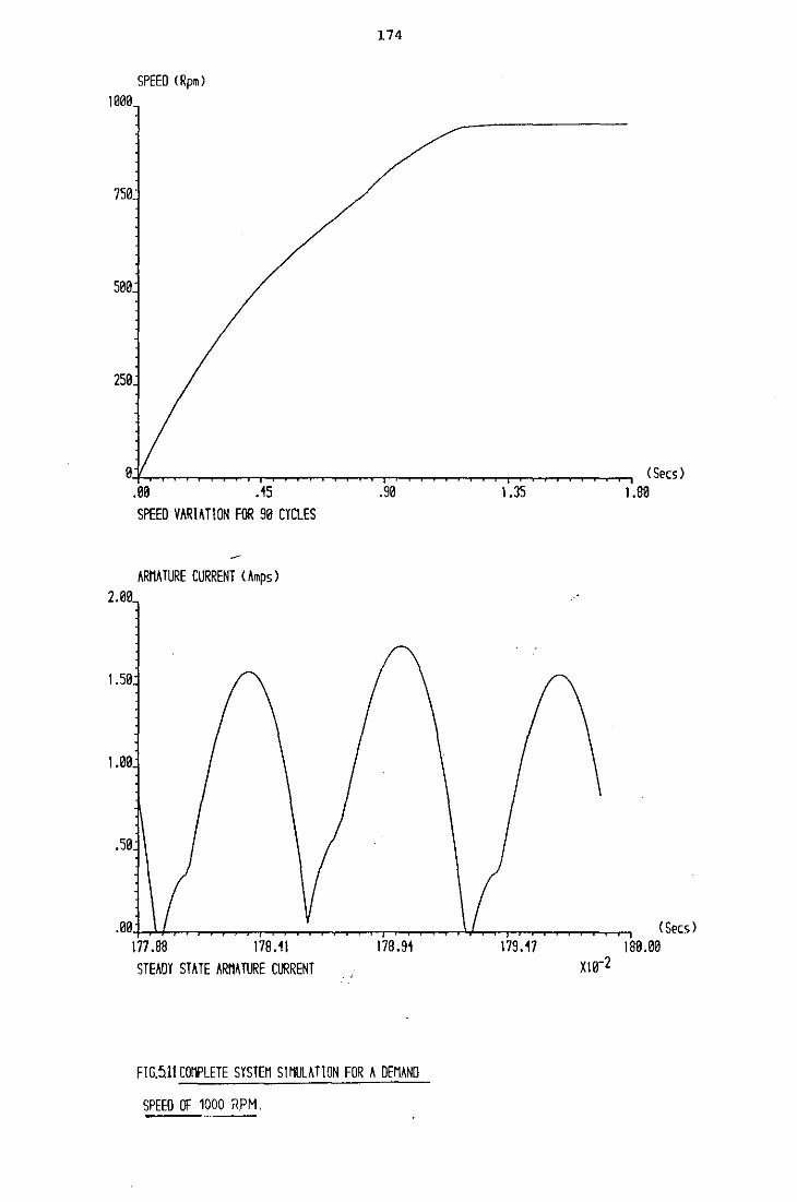
174
SPEED (Rpm) 1e00
7Se
see
2Se
SPEED VARIATION FOR 9e CYCLES
ARMATURE CURRENT (Amps ) 2.0e
l.Se
.se
.ee-f--.'..,_,..,....,~~.......,.~~~~~..,~~~Jo..f-,~,-.-.,..,..~~~...... <Secs) 177.88 178.i1 178.9i 179.17 18Ue STEADY STATE ARMATURE CURRENT
FIG.511 COMPLETE SYSTEM SIMULATION FOR h DEMAND
SPEED OF 1000 RPM.
175
CHAPTER 6
CONCLUSION
In the foregoing chapters, mathematical models of various items
of plant for a limited-size power supply system have been developed.
In Chapter 2, an isolated generator was modelled using the phase
reference frame and various balanced and unbalanced load/fault
situations were simulated. In Chapter 3, the generator model was
incorporated into a parallel-connected multigenerator network.
Both diakoptic and conventional mesh analysis were used to model the -....
system and various load fault situations were simulated. The predicted
results were shown to be identical and it was established that mesh
analysis becomes increasingly more laborious as the complexity of the
network increases. In this respect, the computational efficiency for
the diakoptic approach, expressed in terms of both computer run-time
and core store, was significantly better than when using mesh analysis.
In Chapter 4, models for both a 3-phase full-wave uncontrolled diode
bridge and a controlled thyristor bridge were developed. The
theoretical performance of the thyristor bridge for various trigger
angles was investigated. Chapter 5 described a model for a thyristor-
controlled DC drive with both open-loop and closed-loop control. The
predicted results for the open-loop system were compared with experimental
results obtained on a 0.25 kW DC motor and a laboratory-scale AC/DC
converter bridge, and close correlation was observed between the
results. The closed-loop system, which incorporated speed, current and
power feedback loops, had a small steady-state error between the demand
speed and the actual speed, probably due to the controller and the motor
both being nonlinear and a limit-cycle situation21 becoming highly
probable. A detailed investigation of this effect is outside the
scope of this thesis and could clearly form the basis for further work.
176
In the author's opinion the closed-loop system comprising only linear
amplifiers and neglecting saturation should be studied initially, using
familiar analytical techniques. The nonlinearities can then be
introduced, with conventional nonlinear system techniques being used
in analytical considerations of the resulting system.
6.1 Extension of the Work for Interconnected Items
Although the models for individual items of plant have been
discussed in some detail, the practical situation of a limited power
system requires the interconnection of a number of these items. To
illustrate this, the formulation of an interconnected system such as
that shown in Fig. 6.1 will be discussed briefly. Using a diakoptic
approach, the network of Fig. 6.1 may be torn apart at the bus bars
to comprise torn networks formed by the generators, the AC load
network, the DC thyristor drive and the diode bridge which feeds the
DC load. The system equations for the entire network can then be-
obtained using the diakoptic procedure described in Section 3.2.
Re-writing the diakoptic equation for a parallel-connected network
gives,
pi =L-l{U-Ct [c L-lCtLJ-lc L-l}rE -(R +G )I J m m mL mLm m mLm Lm m m m
(3.46)
where the vectors and matrices of the equation take the various forms
indicated below:
(a) 1 t 1 t I t I t I E I E •E b . d 'E h l' generator 2• AC load• Diode r~ ge, DC t yristor driv<
is the impressed voltage vector where E E generator 1' generator 2'
EAC d' E . d br'dge and EDC h d . represent respectively loa D~o e ~ t yristor r~ve
the impressed voltage vectors of the torn networks of generator 1,
generator 2, the AC load network, the Diode bridge with its DC load
and the DC thyristor drive.
(b) I m
177
= [It : It :It generator•! generator 2, AC
I t I t J 1 ·I ·b 'd .I h d · cad, Diode. r~ ge1 DC t yristor r~ ve
where I is the mesh current vector where I I 2 , m generator 1' generator
IAC 1 d' I br'dge and IDC d . denote respectively oa Diode • thyristor r~ve
the mesh currents corresponding to the torn networks of generator 1,
generator 2, the AC load network, the diode bridge with its DC load
and the DC thyristor drive.
(c) CmL and C~ represent respectively the current transformation
between the mesh and link networks and its transpose. The
formation of CmL i~ similar to that given in Section 3.2.
(d) The L, R and G matrices take the block diagonal form,
Z=
Note:
z generator 1
z generator 2
ZAC load
z Diode bridge
ZDC thyristor drive
where z denotes L, R or G and the suffixes indicate the items of
plant. It remains to evaluate the individual blocks which
comprise L, R and G for each item of the plant.
The rotational inductance matrices GAC load' GDiode bridge and
GDC d . , for the AC load network, the diode bridge thyristor r~ve
including its DC load and the DC thyristor drive respectively
are all null matrices.
The R, L and G matrices for a single generator and the R, L
matrices for the AC load network are given respectively in Figs. 3.6 and
3.7. However, the Rand L matrices for the diode bridge and the DC
thyristor drive, given respectively in sections 4.1 and 5.1, need to be
178
modified, since in these sections R and L are derived by determining
the conducting meshes which may or may not correspond to the currents
of the torn network of the bridge. This may be explained by consideration
of the torn network of the diode bridge circuit including the DC load,
shown in Fig. 6.2. The analysis of a diode bridge, given in section
4.1, leads to the formulation of state equations which are of order
1 or 2 depending on the number of conducting meshes. The conducting
meshes are as shown in Table 4 .1.
Re-writing the state-variable equation, gives
E +V = Z I m m mmm (4. 2}
Suppose, two conducting meshes exist (i.e. in the case of
commutation! and let the conducting mesh currents be Iml and Im2 •
The current vector I then takes the form, m
I m = [Iml Im2] t
where the suffixes ml and m2 do not correspond to any particular
conducting loop or loops. For example, when mesh 1 of Table 4.1
conducts, Iml will represent mesh. current 1, while Im2 will be zero.
However, when meshes 1 and 2 conduct together, Iml and Im2
will
represent their respective mesh currents. It is thus seen that Iml
and Im2 change as the conduction pattern changes.
In a diakoptic approach, the state equation for the torn
network of the diode bridge circuit still takes the form ·given by
equation (4. 2) • In addition, the formulation demands that the
current vector [Iml Im2Jt should always represent the branch currents
corresponding to branches RP and YQ, i.e. irD and iyo· The essential
feature is therefore to determine a suitable transformation so that
the current vector always consists of ird and iyo· The same argument

179
applies for the torn network of the DC thyristor drive network.
However a detailed discussion· illustrating this topic will not be
attempted.
Although the extension of the work for interconnected items
was restricted to the mathematical formulation for the system shown
in Fig. 6.1, it is very general and indeed any complicated parallel
connected network can be modelled by a suitable formulation, to enable
its transient and steady-state performance to be investigated.
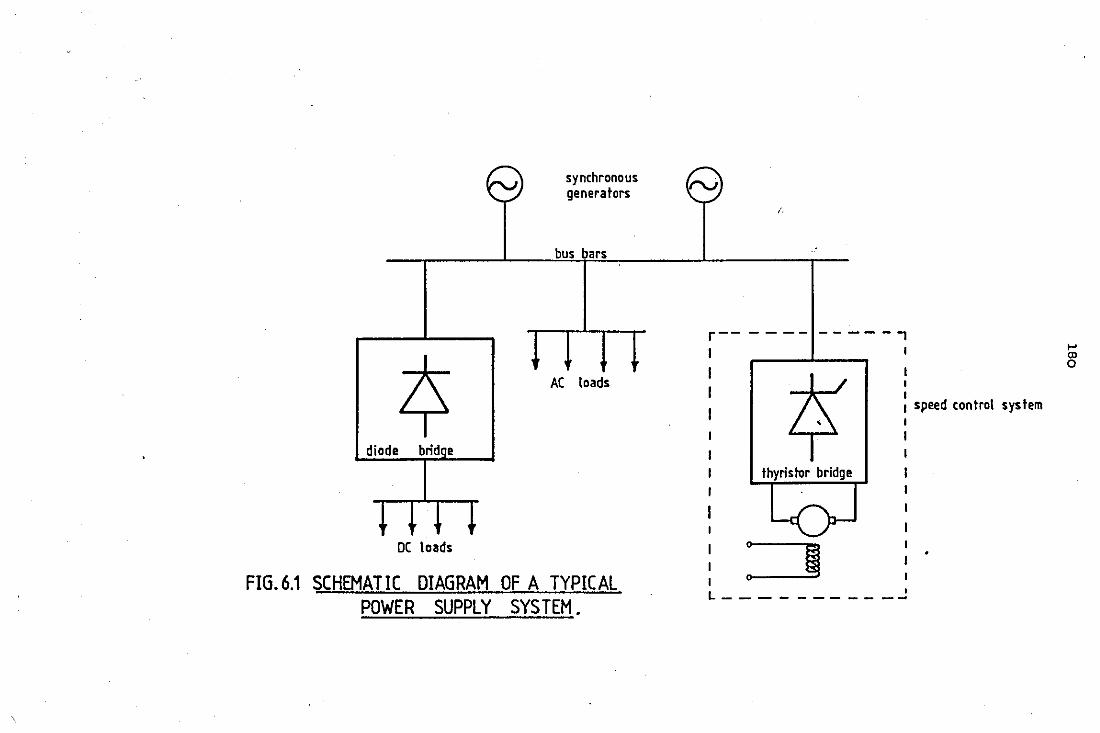
diode brid e
DC loads
synchronous generators
bus bars
AC loads
FIG.6.1 SCHEMATIC DIAGRAM OF A TYPICAL POWER SUPPLY SYSTEM.
r------ -----,
thyristor bridge
I I I 1 speed control system I
I
l----------..!
.... (l)
0
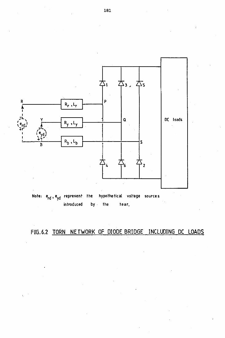
181
..., r- .., .... ., r-1 3 • ~5
R I I p
1 I Rr • Lr I I I ... y J I a. DC loads ' rd} l IRY,LY I .... ,:::'"-, .
I I ~d\ I ' I . +"'' I I
B I Rb , Lb I s
., ... ., r .., sz 4 6
Note: erd, eyd represent the hypothetical voltage sources
introduced by · the tear,
FIG.6.2 TORN NETWORK OF DIODE BRIDGE INCLUDING DC LOADS
182
REFERENCES
l. ADKINS, B: 'Transient theory of synchronous generators connected
to power systems', Proc. I.E.E., 1951, 98, Part II, pp. 510-523.
2. BLONDEL, A. E: 'Synchronous machines and converters', McGraw
Hill Book Co., 1913.
3. DOHERTY, R.E. and NICKLE, C.A.: •synchronous machines, an
extension to Blondel's two reaction theory', Trans. A.I.E.E., 1926,
Vol.45, pp. 974-987.
4. PARK, R.H.: 'Definition of an ideal synchronous machine',......---------
General Electric Review, 1928, 31, pp. 332-334.
5. PARK, R.H.: 'Two reaction theory of synchronous machines -
Part I', Trans. A.I.E.E •. , 1929, 48, pp. 716-730.
6. PARK, R.H.: 'Two reaction theory of synchronous machines -
Part II', Trans. A.I.E.E., 1933, 52, pp. 352.
7. CONCORDIA, c.: 'Synchronous machines', John Wiley and Sons, Inc.
New York, 1951.
8. HWANG, H.H.: 'Unbalanced operation of ac machines', Trans. I.E.E.E.,
1965, PAS-84, pp. 1054-1066.
9. HWANG, H. H.: 'Unbalanced operation of three phase machines with
damper circuits', Trans. I.E.E.E., 1969, PAS-88, pp. 1585-1593.
10. CHING, Y.K. and ADKINS, B.: 'Transient theory of synchronous ~
generators under unbalanced conditions', Proc. I.E.E., 1954,
101, Part IV, pp. 166-182.
11. SUBRAMANIAM, P. and MALIK, O.P.: 'Digital simulation of a
synchronous generator in direct phase quantities', Proc. I.E.E., .~ .., -
1971, Vol.l8, 1, pp. 153-160.
12. SMITH, I.R. and SNIDER, L.A.: 'Predictions of the transient
performance of an isolated, saturated synchronous generator',
Proc. I.E.E., Vol. 119, 1972, pp. 1309-1318.
183
13. KRON, G.: 'Diakoptics- the piecewise solution of large-scale
systems', Macdonald, 1963.
14. . KETTLEBOROUGH, J, G. , SMITH, I. R. , FERNANDO, L. T. M. and
FANTHOME, B.A.: 'Numerical solution of electrical power systems
using diakoptics', Proceedings of the 4th International Conference
on Mathematical Modelling in Science and Technology, 1983.
15. WILLIAMS, s. and SMITH, I.R.: 'SCR bridge converter computation
using tensor methods', I.E.E.E,, Trans., 1976, Computers- 25,pp.l-6.
16. KRON, G.: 'Tensor analysis of networks', Macdonald {1955}.~
17. KRON, G.: 'Tensors for circuits', Dover Publication, 1959.~
18. KRONBORG, G.: 'Industrial d.c. motor drives', ASEA Journal,
Vol. 48, No.S, 1975, pp.l03-108.
19. ADKINS, B. and HARLEY, R.G.: 'The general theory of alternating
current machines', Chapman and Hall, 1975.
20. HAPP, H.H.: 'Diakoptics and Networks', Academic Press, New York,
and London, 1971.
21. SILIJAK, D •. D.: · 'Nonlinear systems', .. John. Wiley and Sons, Inc.
New York, 1969.
22. KETTLEBOROUGH, J.G.: 'Mathematical model of an aircraft
generator/radar load system', RBX Contract Report, 1980.
23. JONES, C. V.: 'The unified theory of Electri·cal Machines',
Butterworths, 1967.
24, RANKIN, A.W.: 'Per-unit impedances of synchronous machines',~
Trans. A.I.E.E., 1945 1 64, pp. 569-572.

A P P E N D I C E S
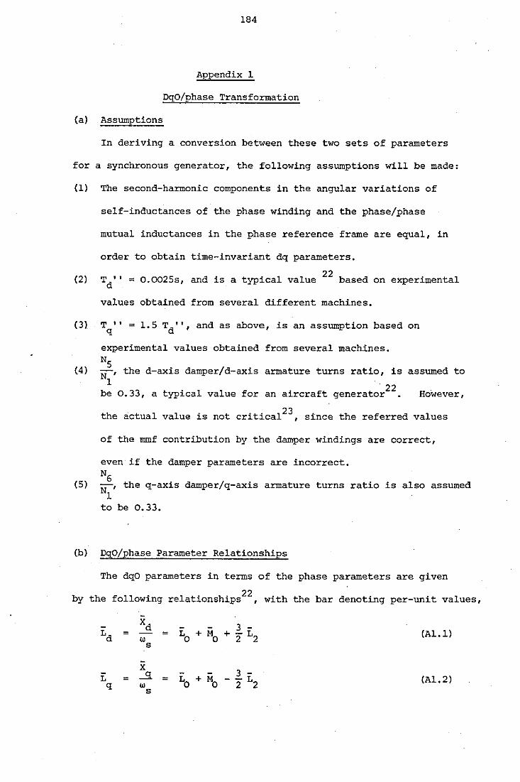
184
Appendix 1
DqO/phase Transformation
(a) Assumptions
In deriving a conversion between these two sets of parameters
for a synchronous generator, the following assumptions will be made:
(1) The second-harmonic components in the angular variations of
self-inductances of the phase winding and the phase/phase
mutual inductances in the phase reference frame are equal, in
order to obtain time-invariant dq parameters.
(2) 22 Td'' = 0.0025s, and is a typical value based on experimental
values obtained from several different machines.
(3) Tq'' = 1.5 Td'', and as above, is an assumption based on
experimental values obtained from several machines.
(4)
(5)
N
N5
, the d-axis damper/d-axis 1
armature turns ratio, is assumed to
22 be 0.33, a typical value for an aircraft generator HoWever,
the actual value is not critica123 , since the referred values
of the mmf contribution by the damper windings are correct,
even if the damper parameters are incorrect. N6 NI• the q-axis damper/q-axis armature turns ratio is also assumed
1 to be o. 33.
(b) DqO/phase Parameter Relationships
The dqO parameters in terms of the phase parameters are given
by the following relationships22
, with the bar denoting per-unit values,
Ld xd 3 -= = Lo + MO + 2 L2 w (Al.l)
s
X 3 -L = ...sl. = Lo + MO 2 L2 q w
s (Al. 2)
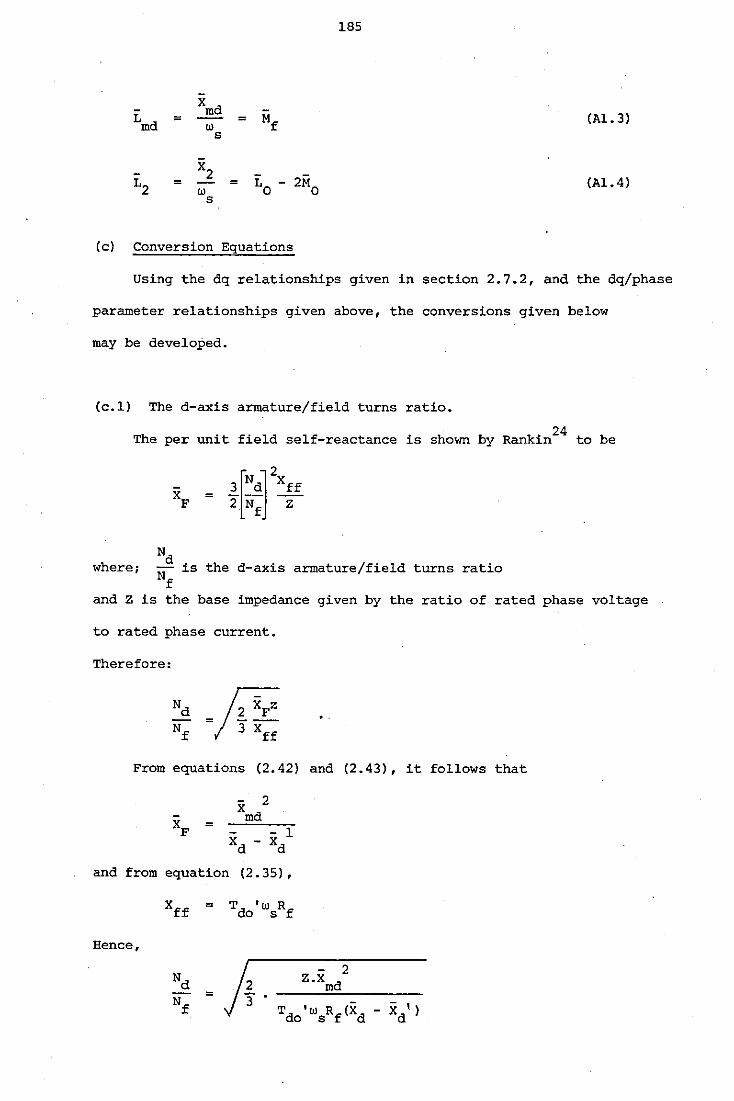
185
Lmd xmd
Mf = = Ill
(Al. 3) s
- x2 2M
0 L2 = = L -Ill 0
(Al. 4) s
(c) Conversion Equations
Using the dq relationships given in section 2.7.2, and the dq/phase
parameter relationships given above, the conversions given below
may be developed.
(c.l) The d-axis armature/field turns ratio.
Th . t f. ld lf . h b k. 24 b e per un1 1e se -reactance 1s s own y Ran 1n to e
=
where; Nd -- is the d-axis armature/field turns ratio Nf
and z is the base impedance given by the ratio of rated phase voltage
to rated phase current.
Therefore:
=~ From equations (2.42) and (2.43), it follows that
=
and from equation (2.35),
=
Hence,
= 2 3
- 2 z.xmd
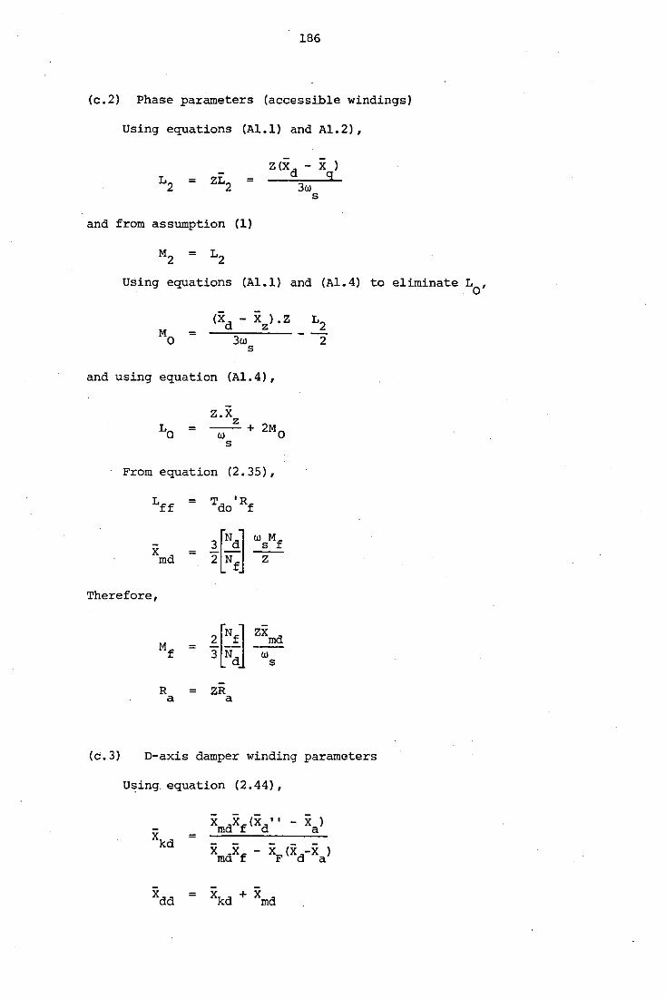
186
(c.2) Phase parameters (accessible windings)
Using equations (Al.l) and Al.2),
= = z cxd - x > q
3w s
and from assumption (1)
=
Using equations (Al.l) and (Al.4) to eliminate L0
,
M = 0
(Xd- Xz).Z L2 3w 2
s
and using equation (Al.4),
z.xz = -w- + 2Mo
s
From equation (2.35),
Lff = Tdo0Rf
xmd l[Nd] wsMf
= 2 Nf z
Therefore,
(c. 3)
Mf ~[~fj zxmd =
3 Nd w s
R = ZR a a
D-axis damper winding parameters
Using. equation (2.44),
= xmif cxd' ' - xa>
xmdxf - XF(Xd-Xa)
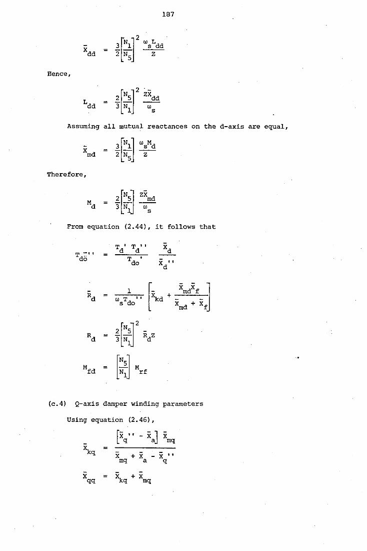
187
Hence,
Assuming all mutual reactances on the d-axis are equal,
Therefore,
From equation (2.44), it follows that
T -·' do =
=
Rd =
Mfd =
1 w T •• s do
~lNsr 3 Nl RdZ
[:~ Mrf
X " d
(c.4) Q-axis damper winding parameters
Using equation (2.46),
[xq'. - xa] X mq
xkq = X + X - X '' mq a q
-X = ~q+ X qq mq
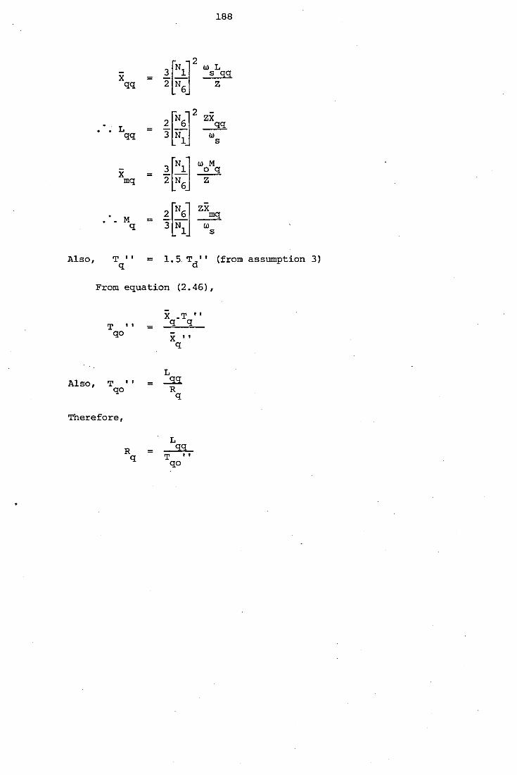
188
~rlr Ill L X = s SS! qq 2 NG z
~~6r zx L = _39:.
qq 3 N1
Ill s
~lNlJ w M X = ~
mq 2 NG z
~~N6j zx M = _!lE.
q 3 N1 Ill s
Also, T '' = 1.5 T '' (from assumption 3) q d
From equation (2. 46)'
X .T 11
T •• = q q
qo X '' q
L Also, T •• = _.ss.
qo R q
Therefore,
L R =
qq q T ••
qo
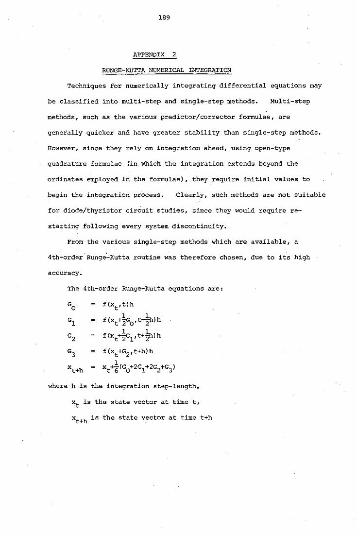
189
APPENDIX 2
RUNGE-KUTTA NUMERICAL INTEGRATION
Techniques for numerically integrating differential equations may
be classified into multi-step and single-step methods. Multi-step
methods, such as the various predictor/corrector formulae, are
generally quicker and have greater stability than single-step methods.
However, since they rely on integration ahead, using open-type
quadrature formulae (in which the integration extends beyond the
ordinates employed in the formulae), they require initial values to
begin the integration process. Clearly, such methods are not suitable
for diode/thyristor circuit studies, since they would require re-
starting following every system discontinuity.
From the various single-step methods which are available, a
4th-order Runge-Kutta routine was therefore chosen, due to its high
accuracy.
The 4th-order Runge-Kutta equations are:
=
=
=
=
=
f(xt,t)h
1 1 f(xt¥o•t7Jh
1 1 f(xt+2G1 ,t+2fllh
f(xt+G2 ,t+hlh
1 xt~(G0+2G1+2G2+G3 )
where h is the integration step-length,
xt is the state vector at time t,
xt+h is the state vector at time t+h
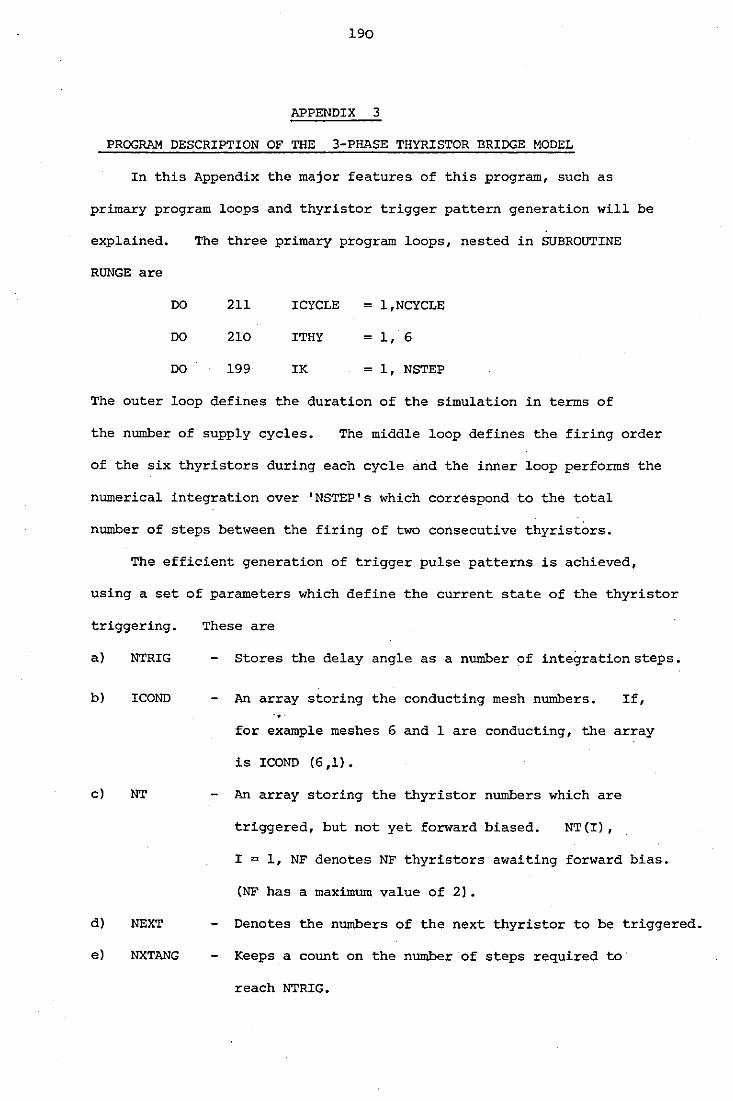
190
APPENDIX 3
PROGRAM DESCRIPTION OF THE 3-PHASE THYRISTOR BRIDGE MODEL
In this Appendix the major features of this program, such as
primary program loops and thyristor trigger pattern generation will be
explained. The three primary program loops, nested in SUBROUTINE
RUNGE are
DO 211 I CYCLE = l,NCYCLE
DO 210 !THY = 1, 6
DO 199 IK = 1, NSTEP
The outer loop defines the duration of the simulation in terms of
the number of supply cycles. The middle loop defines the firing order
of the six thyristors during each cycle and the inner loop performs the
numerical integration over 'NSTEP's which correspond to the total
number of steps between the firing of two consecutive thyristors.
The efficient generation of trigger pulse patterns is achieved,
using a set of parameters which define the current state of the thyristor
triggering. These are
a) NTRIG Stores the delay angle as a number of integration steps.
b) ICOND An array storing the conducting mesh numbers. If, .. for example meshes 6 and 1 are conducting, the array
is ICOND (6,1).
c) NT An array storing the thyristor numbers which are
triggered, but not yet forward biased. NT (I) ,
I = 1, NF denotes NF thyristors awaiting forward bias.
(NF has a maximum value of 2].
d) NEXT Denotes the numbers of the next thyristor to be triggered.
e) NXTANG Keeps a count on the number of steps required to
reach NTRIG.
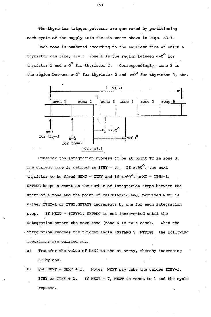
191
·The thyristor trigger patterns are generated by partitioning
each cycle of the supply into the six zones shown in Figs. A3.1.
Each zone is numbered according to the earliest time at which a
thyristor can fire, i.e.: Zone 1 is the region between ~=0° for
thyristor 1 and ~=0° for thyristor 2. Correspondingly,. zone 2 is
. 0 0 the region between ~=0 for thyristor 2 and ~=0 for thyristor 3, etc.
I· 1 CYCLE . I Tl zone 1 zone 2 jzone 3 zone 4 zone 5 zone 6
I I I I I I . !
i l Tl ~<60°
~=0
for thy=l ~=0 ~>60°
for thy=2 FIG. A3.1
Consider the integration process to be at point TT in zone 3.
The current zone is defined as ITHY = 3. 0 If ~~60 , the next
thyristor to be fired NEXT = ITHY and if ~>60°, NEXT= ITHY-1.
NXTANG keeps a count on the number of integration steps between the
start of a zone and the point of calculation and, provided NEXT is
either ITHY-1 or ITHY,NXTANG increments by one for each integration
step. If NEXT = ITHY+l, NXTANG is not incremented until the
integration enters the next zone (zone 4 in this case). When the
int~gration reaches the trigger angle (NXTANG ~ NTRIG), the following
operations are carried out.
a) Transfer the value of NEXT to the NT array, thereby increasing
NF by one,
b) Set NEXT = NEXT + 1. Note: NEXT may take the values ITHY-1,
ITHY or ITHY + 1. If NEXT= 7, NEXT is reset to 1 and the cycle
repeats.
192
c) If the new NEXT = ITHY -1, then
NXTANG = NSTEP + !STEP.
If the new NEXT= ITHY, then
NXTANG = !STEP.
If the new NEXT < ITHY-1, this indicates that the range of firing
of NEXT has passed and NEXT is updated to NEXT+l i.e.: move on to
the next thyristor to be fired.
When NXTANG ~ NTRIG, thyristor NEXT has been triggered and a
check is made to see whether it is forward biased VD(NEXT)>O.
it commences conduction and the mesh differential equations are
modified accordingly.
If so,
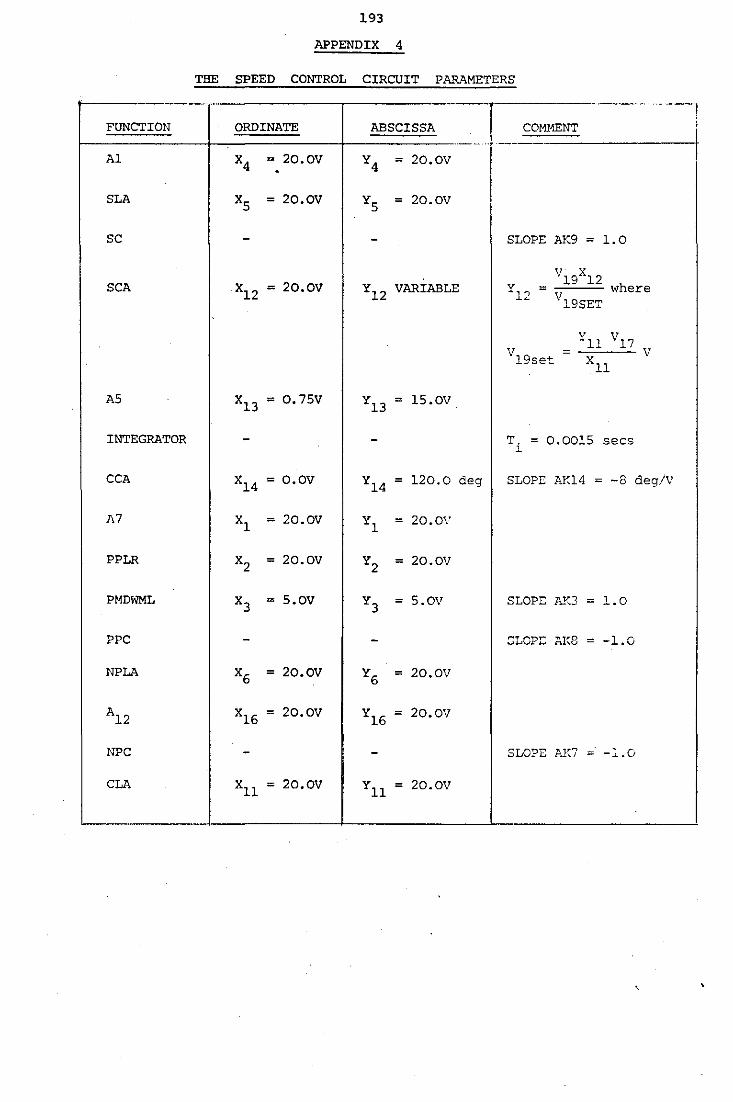
193
APPENDIX 4
THE SPEED CONTROL CIRCUIT PARAMETERS
- ~- .. ---- ··--, FUNCTION ORDINATE ABSCISSA COMMENT i
I ···---··· --·
Al x4 = 20.0V y4 = 20.0V . SLA xs = 20.0V Ys = 20.0V
se - - SLOPE AK9 = 1.0
SCA xl2 20.0V yl2 VARIABLE V vl9xl2
where = = ... 12 Vl9SET
V vl7 -n V = V 19se~ xll
AS xl3 = 0.75V yl3 = lS.OV
INTEGRATOR - - T. = 0.0015 secs l
CCA xl4 = o.ov yl4 = 120.0 deg SLOPE AY-14 = -8 deg/V
A7 xl = 20.0V yl = 20.0\'
PPLR x2 = 20.0V y2 = 20.0V
PMDWML x3 = s.ov y3 = s.ov SLOP!: AKJ = l.O
PPC - - :JLOPI: AK8 = -1.0
NPLA x6 = 20.0V y6 = 20.0V
Al2 xl6 = 20.0V yl6 = 2o.ov
NPC - - SLOPE AK7 = -l.O
CLA xll = 20.0V yll = 20.0V

APPENDIX 5
LISTING OF COMPUTER PROGRAMS
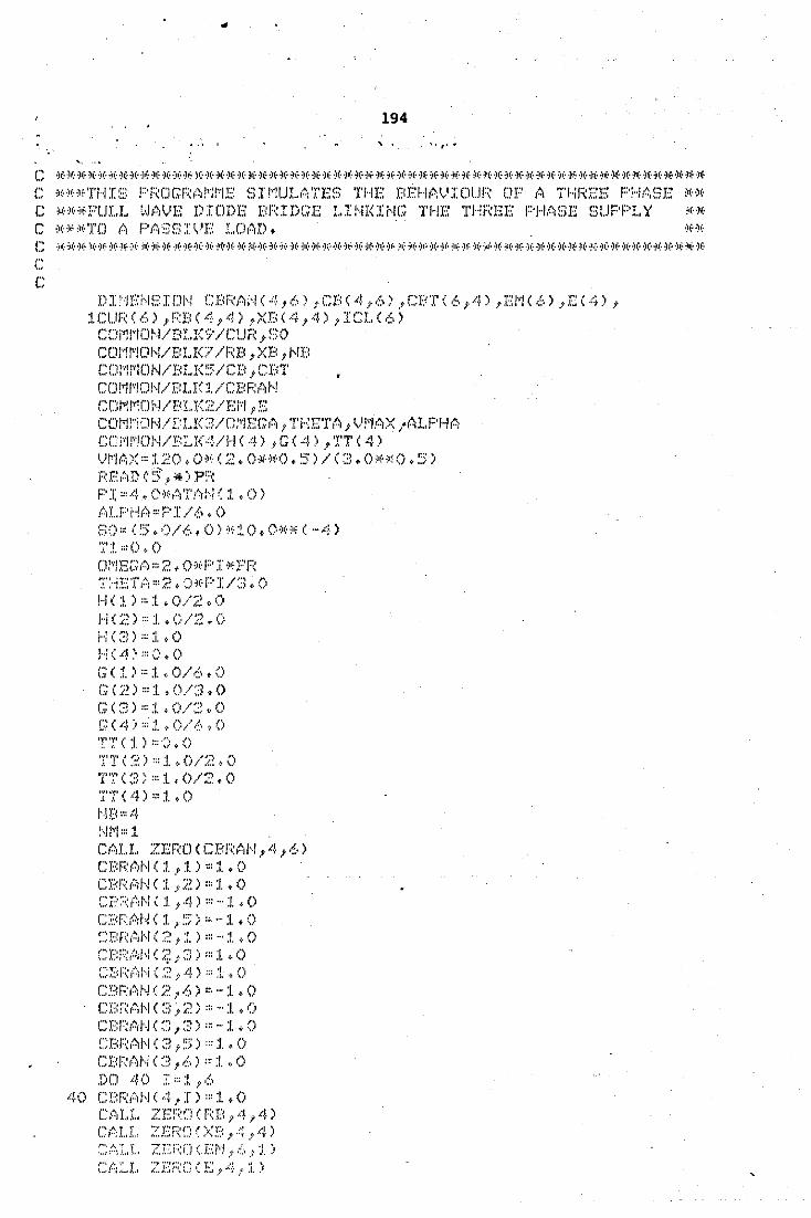
..
194
' . . . ,. ~
~.. ". c ~~i~**~~~f*i~i~***~~****if*****~f*if~~if***~f*if1f***if*if*if***~f****~*~f**~fif*** C ~(··:n:·)f·TH I ~3 F'F~OGF~,-:~!''lfl'IE S J !''!t.JL,~:'I'E~:~ THE F{E:Ht:;V I DUI:~ DF'· t:\ THHEF·: F'Ht:.~3E *··)(·
C ***PULL WAVE DIODE BRIDGE LINKING THE THREE PHASE SUPPLY ** C ***TO A F)ASSIVE ! .. DAD. ** (: ~f***~f*~f0~*if~f*ifi(**if**if*~~ifif*i0#if*~f*9~ififif*i~~f~~**~~~f*0fifif*if*~~if**if**~f***
(., ·'
DI!iSi,ISION CBRA:\!C4 1 6) 1 CB(4 1 6> 1 CBT<6 1 4) 1 EMC6) 1 EC4>, 1CLJR(6) 1 RBC4 1 4>,XBC4 1 4) 1 ICLC6) COMJ10~1/Br.K9/CUR 1 !30 CCW!!''!CJ!-..l/I-:-:L1(;7 /F~B ,XB I t'-fE: COMriON/BLK5/CB 1 CBT CD!~"l/''lD!-..1/ DI..X( :!. /CDr;,;H CDI"'li'"!DH/BLK~~/E! ... J,E C01'1r!,]J ... I/tLK:3/Ci''!EGr~, 1 TEET,~ 1 'v'r1r~X /r.~l.PHA
CCl1MON/BLK4/l··I(4) 1 G(4) 1 TT(4) VMAX=120.0~~(2.0**0•5)/(3~0~~M0.5) '"•['·"" I''l '!I:::- . •. pr"o l'\,',',1"),,. ~.M':' i *), (\
F'];:::4-.0:'f·t~Tr1H( :1. ~O)
tli .. PHt-~:::PJ/.~,. 0 S0=(5.0/6,0)~fiO~O*~e(-4)
'J' :!. "' () •· ()
H ( :!. ) " :l • 0 /'/..: , 0 H(~;~) :::J. +G-/::?. .. 0 H(a>===:i..O H(4~':::(},()
G ( :!. ) ::: :1. i· O,l 6 * 0 G ( L!.) ::: :1. ~ 0/3 • 0 G ( ~:!) ::: :! .• 0/~? (· 0 G ( 4) ===· :! . • 0/ <:~ "0 '!'T < j,) :::<J y 0 TT ( ~.?.) ::: :J.. 0/~? -~ () TT ( ~3) ::: 1 { 0./2. 0 TT< 4) ::::1..0
~·!El"' 4
CALL ZERO<CBRAN 1 4 1 6) CDI'<:AI-·1 ( :1. _. :1. ) "' :1. , 0 CX:<F:i'•i'··! ( :1. -'::?.) '" :1. , () cp;:;~P~I\1 \ :1. 1 .(.!) ::: ... :1. • ()
C~0F\:PJ!···! ( :1. ~ ~;;) ::: ... :l + 0 ~:::I-:~f::(~rl··.f ( 2, :i.) ::: ... :!. • 0 CE:F:/~~1---r ( ;.~~ 1 ~:J > ::: l "0 CE;F;~~:':·ii··.J ( ~.:: .~· 4) ::::!. ~ 0 C~::~F:1~H (? _. 6) =~· ... :1. • 0 CBF~:P;/\1 < :;~ }'?) ::: ... :1. • 0 cr::H(ii··.J < ~:; ,:~~ > =~ ... :J. .. () CBF~~~I\1 ( ~=~ 1 ;::; ) ::: l • 0 CDF::r;/"--J < 3 t ~_:.) ::: :L (· 0 DD -40 I::; :1. l'~~
40 CBRANC4 1 J):::1.0 CAl .. L. ZEF~[)(F~B 1 4 1 4) CAI .. I .. ZER!J(XB 1 4 1 4) Ct\·; .. I .. ZEF;;D < Ei''l, .1:.} :l.)
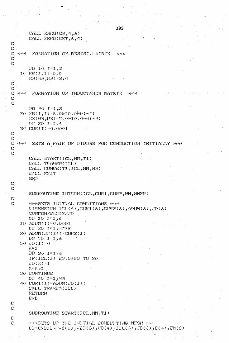
(., .,
(., ·'
c
c c
CALL ZEROCCB 1 4 1 6) CALL ZEROCCBT 1 6 1 4)
DD :1.0 :J::::l.tJ :1. C F<D C I _; I ) " 0 •· 0
195
C *** FORMATION OP INDUCTANCE MATRIX *** c c
c
DO ::>.0 I"':i._,::l 20 XB<I,I>==8o0*10.0**(-4)
XBC!,!B 1 ~!B)=5 •. 0~~10.0**(-4)
:]0 CUF<CJ):::O,OOO:I.
C *** SETS A PAIR OF DIODES FOR CONDUCTION INITIALLY *** c c
c c
c
CAl.L STAR1'CIC1. 1 NM 1 1'1) C(.•,LL TF(tJI·I~')I"I ( I CL) CALL RUNGECT1,ICL,NM,NBl Ci~J!..l.. I.:: X IT El•!!)
SUBROUTINE INTCONCICL,CUR1 1 CUR2,NM 1 NMPR>
r: ~0*~GSET~J I~I:ET~Aid CONDIT:[ONS **~~
( .. ·' ( .. ..
c
DI!~ENSION ICLC6) 1 CUR1(6) 1 CUR2C6> 1 ADU!~(6) 1 JDC6) ~:;C]'1li\'!Dl,!./BLX< :i. ?/ 1.TD DD 1.0 I"'J. 1 6
10 ACUMCI)m(),()001 DD ;:,~o I'" 1. 1 1··1i"IF'F(
20 ADUMCJDCill=CUR2Cil llD !')0 I" :1. 1 6
::;o ,!!)(I) m()
I->l DD 30 :r::::J. ?6 IFCICLCil.EQ,OlGO TO 30 ~.TD( X<)::: I J<::;I<+:l.
::l 0 ;:; CJ cl T I 1··/l.J E DD 40 I::: 1 t /",!Jtl
40 CUR:I.CI)mADU~CJllCill C/~1LL Tf~td\1~3!.,.i ( I CL) i":ETLJF::I··I EHD
r ***'5ETS UP TH2 INITIAL COHDUCTING MESH **'' DI!~'lE:!·IS1DI"·i ~.)D ( 6) 1
1-./D,::J ( 6) 1 1)1':: ( 4_) l ICL ~:,f.,) , .. :rD< 6) JE ( ·4 > 1 E!'1 < 6)
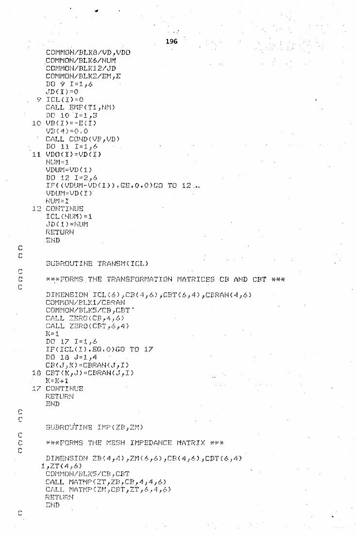
c c
..
COMMON/BLK8/VD,VDO CD/'//'"/DN/BLI<.~·/~/U/1 CDl'/J"/OJ·.J/Bl..l< :1. ;:,;,JI) COJ•·JJ··JCJ/•1/BLI<:UE/~ 1 E DO 9 J:::::J. 1 6 ,,m( I) "'0
'? I Cl..\ I) "'0 c,~rLL EI'·IF ('1':1. ,t.J!•"i) DD :1.0 J>rr:J. _,:;;
:1.0 VB (I ) =- E \I l I.JB ( 4 ) ::: 0 V ()
CALL COt~D<VB 1 VD) DD :!.:/. I=:!. 1 !•
11 VDO <I l "VD CO /•11..1/'Jr":J. VDUJ•·;" VD ( :1. ) D 0 :!. ::.: J><' ·' .:.,
196
If' C CVDLJ/'"J .. ·Vl)( J) l, GE. 0. 0 l GCJ TO :1.;~ •. v m.m '" ··.m < I l
I CL ( !--JU!v!) ::: 1 ,}!)( :1.) =!"·-!1..11"'1 I'~E:TUF::H
Ei\iD
SUBROUTINE TRAHSMCICLl
C ""''(:·!•·I.-'DF::J'l~') THE TF:td··lf:lFClF:J•!A'l'IDI··I J·•J!'rTI'UCE!:l CB AI•!D CBT lHH~
c
c c
c
DIMENSIOH ICLC6l 1 CBC4 1 6l 1 CBTC6 1 4l 1 CBRAHC4 1 6l CO!i!~ON/BI.K1/CBRAN
COMMON/BLK5/CB,CBT' CALL ?EROCCB 1 4 1 6> C:ALL ZERO(CBT 1 6 1 4) 1{::: :l DD :1.7 I"':1.,6 IPCICL<Il.EQ.OlGO TO 17 DD 11:\ ,,r,, :1. 1 4 CBCJ,Kl=CBRANCJ 1 Il
18 CBTCK 1 Jl=CBRANCJ 1 Il I<"'K+1
F~ETl.J!::~!···l fl.IJ)
r •••FORMS THE MESH IMPEDAHCE MATRIX MNN c
, .. \,,.
DIMENSIDH ZBC4 1 4l,ZMC6 1 6l 1 CBC4 1 6l 1 CBTC6 1 4) 1 1 ZTC4/•l COM~!Ol,I/Bt.K~5/CB,CBT
CM.L J•·if; '!'!'/!"' \ ZT 1 ZE<, CB, 4 J 4, 6) CtiLI., 1\'l(:-I'I'!''lP ( zr··! ,Cf:'I' tZT ,b /'4 1 6) F::ETUF:.:!··.J ::Jm
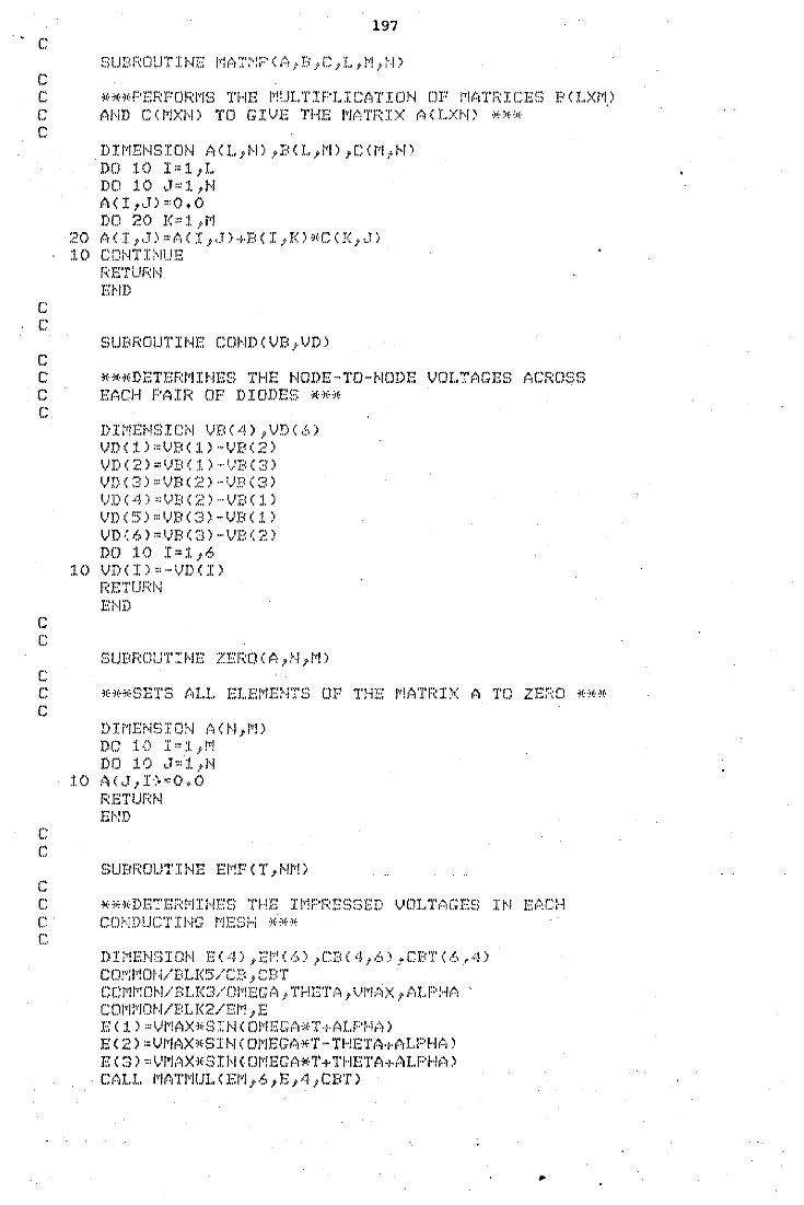
197 c
c C •••PERFORMS THE MULTIPLICATION OP MATRICES BCLX~) C Al-,iD C ( 1'/XI·,I) TO GI'JE THE I''I<':TF:IX A O..Xr,f) ·:0\·)H<·
c
C' c
c
DIMENSION A<L 1 Nl,BCL 1 Ml 1 CCM,Nl DO 10 I•l 1 L DO 1.0 cl"'l.,l'l A<I,cO"O•O DO :~0 I<'" :1. .•' f'l
20 ACI 1 Jl•ACI 1 Jl+B<I 1 Kl•C<K,Jl :1. 0 C Dl·n' I '•11..1 E
f\ET\.Jf(l·l El' ID
SUBROUTINE CONDCVB,VDl
C •••DETERf'IINES THE NODE-TO-NODE VOLTAGES ACROSS C EACH PAIR OP DIODES *** c
c ("
c
D I i'IEI,!f:) I Ci•l VD ( '·!) 1 VD ( .s l VDC1l•VBC:I.l-VBC2) VD<2>~VB(1)-·VB(3)
VDC3)=VBC2)-VBC3> Vl)(4)::VBC2)-·VBCl.) VDC5l•VBI3l-VBC:I.l VD(6l=VBC3l-VBC2l DO 10 I • :1. ;6
:1.0 VD (I l '"···VD< I l 1'\ETUf\f'.l EHD
SUBROUT:NE ZEROCA 1 N1 Ml
C ~(·1(·-i(·SET~~ f.1I..!.. EI .. El.,IEHTS OF THE J't!ATF~I)< A 'l'D zr::::~o 1~:~(·~(·
c
(''
c
DIMENSION A!N 1 Ml DC 10 J::::t,!.,! DO 10 cb :1. ,1··1
:!.() r~c • .r,:o~o.o F:ETUf\~1
EI•:D
SUBROUTINE EMPIT,NMl
C ·)(··i.:··l~:DETEi-~J···JIHF:n TI··1E Il.,!PF~Esr:;r:D VD!..T/:!Gf:.:f:) I~,! I·:·:t-:CH r CO~!DlJCT:[NG MESl-1 **~f (".
DIME~i!3IO~I E(4) 1 EM(6),CB(4,6>,CBTC6r4> C(J;Y;JY!(JJ·.j/E~I..I<5/CI~ t CDT COM~O~I/Bt.K3/Cll~EGA 1 THE1'A 1 VMAX 1 ALPHA CCli'II"IDI··I/BI..lCUEI'I ,E Elll=VMAX•SIHCOMEGA•T+ALPHAl EC2l=VMAX•SINCOMEGA•T-THETA+ALPHAl E C cl) "'VI'Ii~X)(·f:>II>I I DI"!ECAl"T+THETA+,~l..PHA) Ct;LI.. I'Wl'i''IUL I El''l t <-• 1 E 1 4 1 Clrf)
..
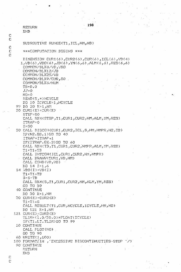
(., ,,
(., ,,
c
(''
c
FmTUF:~J
El ID
198
SUBROUTINE RUNGE<Tl,ICL,NM,NBl
DIMENSION ClJF~1(6>,CtJR2(6) 1 ClJF~C6) 1 ICL(6) 1 VBC4) 1 1 VDC6l 1 VDOC6) 1 JDC6l 1 YMC6 1 6l,ALMC6 1 6l 1 RESC6 1 6)
COMMDN/BLK8/VD 1 VDO CD/'WIDH/BI.J<LY cTD CCP!!''l0ri/Bl..I<i.':0:/VB CCJI"WIDH/BLI<9 /CUI~ 1 SO CDI'ii'ION/Bl .. I<6/i··JUI'I TB:::O+O ,J,.T:::O I'ID" 0 r::EMl < ~) _, ,>(· l J·.JCYCLE DO 10 ICYCLE=1 1 NCYCLE
'?? DD £.~0 I\::::!._tt,W\ :::;:o cum. < ro '" c t.m o< >
~:;TEF'===BO
CALL RI<4CSTEP 1 T1 1 CUR1 1 CUR2 1 HM 1 ALM,YM 1 RESl ITF\P,F':::O E;:::f:)O
50 CALL DISCDNCCUR1 1 CUR2 1 ICL 1 S 1 Ni'I 1 NMPR 1 N2 1 TBl IFCI•J;;>,r-:;G,:llGO TO 40 I 'X'f~t~P :::I T::~:AF'+1
(''·'! l "'•"•' !")'~' ''(''I I''IJI""I '''[IJ"•'') ''·l'''f'•'"' A!·~ YJ"I , .. ,, .• C') ,,.J"I,,t ,, f'\,\',o~, ~',}i• ,,,\.~. '\,,,/t.~ .. '\;;:,_yl',: '{',pJ••j,,,/'/f, '•/'~'\.\,~,;;,,
T:l. :::T:i.+TB CALL I l'-!'I'CDI'-1 {:::CL 1 CUf\:!. 1 CUF;~~-~ 1 Hl''l,. r.f! ... Jpr::) CP., I..!.. DFMIW < GUF\ :l 1 VD, ~-·1!'1) Ct1LL CUI-.JD (VD_, VD) DD :1.4 I"' J. t f.,
:1.4 ',JJ)CJ C I) ocV[) C I) T:L :;:Ti+TD B:::~:>· .. TB CALL RK4CS,T1 1 CLm1,CUR2,NM 1 ALM,YM,RBSl GO 'I'D 50
40 CD hiT Ii'-iUE DD ::lO !< "' J. ·' 1··11'1
30 CUR(Kl=CUR2<I<l T :1. :::'I' :J. +B CM .. L !'::E!3l.JLT C 1'1 ,CUf\ ,HCYCLE 1 I CYCLE ,~!l'l 1 1'10) DO :!. ;::~:!. !-(::: :1. ;-1··-l!'"f
121 CURCKl:CUR2CI<l TLIM=C:I..0/50.0)WFLDATCICYCLE) IFCTl.LT,TLIMlGD TO 99
10 COHTII·IUE CALL I"'LD'l' ( 1·10 l GO TO 90
60 I.Jf\ITE ( :1. t :1.00 l FDR~AT!lH ,'EXCESSIVE ., ()()
,I, " •··
90. CDJ·.JT' H'i'...IE r::r:Tur::J·i EJ-.JJ.l
DISCONTIHIJITIES-STOP '/)
..
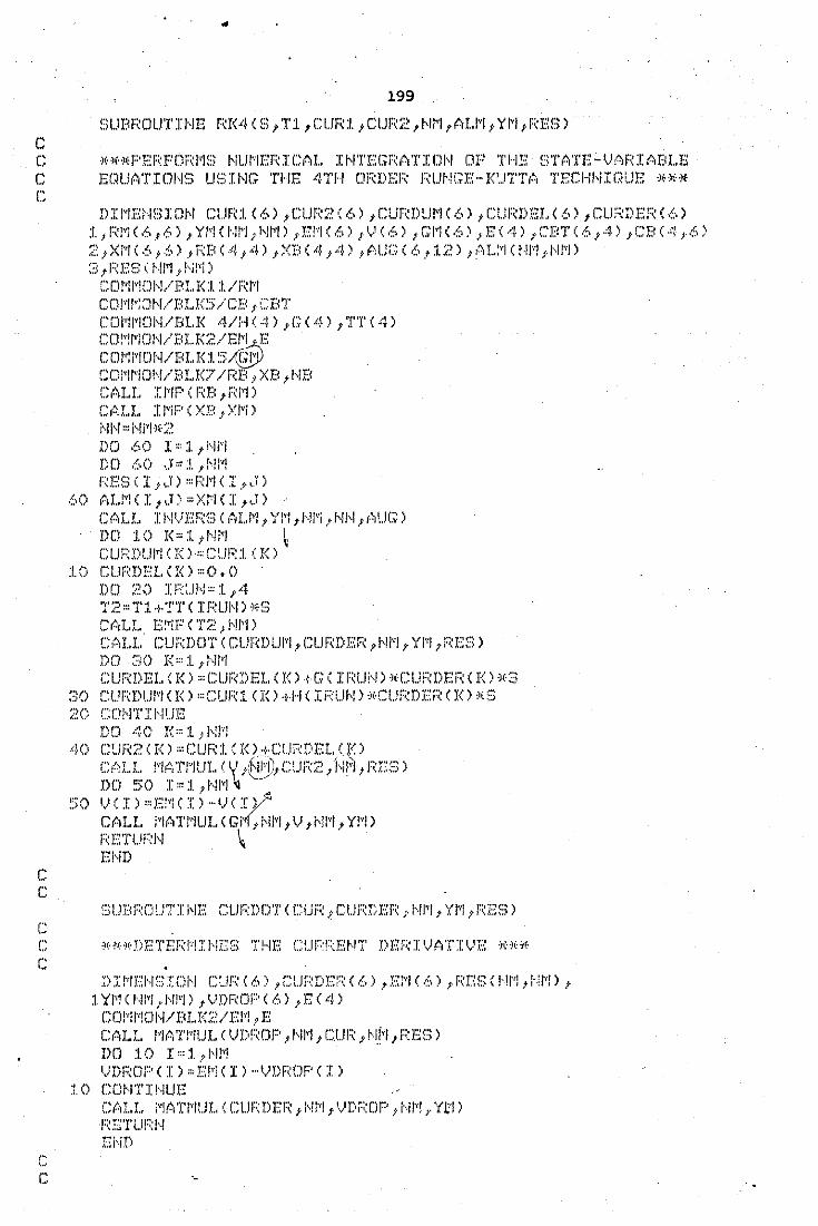
..
199
[>UBFWUT:ITJE m<4 c "', n, c1.m:1., um;:.~ ,1,11'1 ,Al..l'l, YN ,r<E!:> l c C •••PERFORMS NUMERICAL INTEGRATION OF THE STATE-VARIABLE C ECll.JrYI'ICll'-1'3 U!c.:niG THE 4TH OFWEF< FWI·-!GE·-J(! .. .i'l'Tt~o 'lT:CI·-II·iHlUE ·JHHf
I"
(''
c (''
'"
c
c
DIMENSION CUR:I.C6) 1 CUR2C6l 1 CURDUMC6l 1 CURDELC6l 1 CURDER(6) 1 1 RI~C6 1 6) 1 YMC~lM 1 NM) 1 B11C6) 1 V(6) 1 GI1(6) 1 EC4) 1 (:BTC6 1 -4) 1 CBC4 1 6) ~::,xi·rJ ( 6 t·~') .tF~B ( -4 ,t4) ,XB ( 4,4) _tf.;UG ( 6 .t' :1.~~) ;('II .. :"I C J·.JJ.,.!JJ··-!l\'1) ~;5 t F;~ E B ~ l\!1''1 , !"Wi )
CDI'1!I.,lDI,!./BLI<:I. :l./i:~t'l COl1l~JN/BLK~5/CB 1 (:B1' COMMON/BLK 4/HC4l 1 G(4l 1 TTC4) r"(l"''I'''JI'I "''' !"0 /l-'1'"1 r~ ~-' .. , ; h / .t<).,, \..:,.~· 1 .. ~.~':-!!:.·'
CD!"!I.,.ID!\1/BI..I< :1. :~:/\Q!Y CCWII'"iDI·-1/F.<Ll<? /F<B ·' XB 1 I'IB Ctol..l.. I I'll"' ( FW 1 f(l'l l C1~LL I l''iP C XB .t J:~l''i > i"JH ::: i··.JtrJ·)(·~:.~ DD 60 I" :1. 1 i·-Jrl DD .-so .J::: :!. ,1'-!l''' r~x-::!:> < I}" -.r l '" F<l''l < I ... r l
60 ALMCI 1 J)=XriCI 1 J) Cf0LL I J-J!)J.-:·:F:~~:; ( I~ILf''l; Yl''l J 1··1/''i ,.tl-ll·-l.r t:':JUG) DO 10 K•1,NM ~ CUF~DlJJ~CK)=ClJR1CK>
:to curmEL c:o •O. o DO ;".() 1 F'c:.ll'-1 '" :l ; 4 T;;'.•,T:I.+TTC 1PUHl·l(·!3 Crt.iLL. E~''!F C T£.:: 1 !-..!J'"I) CALL CURDOTCCURDUM 1 CURDER,NM,YM,RESl DD ::JO J<::::L,!···il~'i
CURDEI..CKl•CURDEI..Cl<l+GCIRUN)wCURDERCKl•S 30 CURDUMCKl•CUR1CRl+HCIRUNl•CURDERCl<l•S
!5!.JBl~Ol.JT:rNE CLJRI)C)TCC~!JR 1 CtJRI~ER 1 NJ~,YM 1 RES)
X>I~IEI,ISI(JN C~JRC6) 1 C1.JF~DE:~C6> 1 EM(6) 1 RESC~!M,~·fM>, 1YMCNM 1 NMl 1 VDROPC6l 1 EC4l
CDI'ii"!DIVI<l..l<:i.'/E!··r ,E C:t~l.L I''IIY!'J''IUL < VDI'WF' ,1···11"1 1 Cl..JI'< ,HI'I ,r::r:;s l DD :1.0 l> l t !·11'! VDRDF'Cil•EMCil-VDROF'Cil
:!.0 CC::~ITI!-IUE
C:tol..L i''IA'l'I"'I.JL ( Cl.JI'::DER, l'·il''l, 'Jl>fWF' ·' i·-WI ,. Yl:'l l F::':::TLJ!'::I·-1 EHD
.
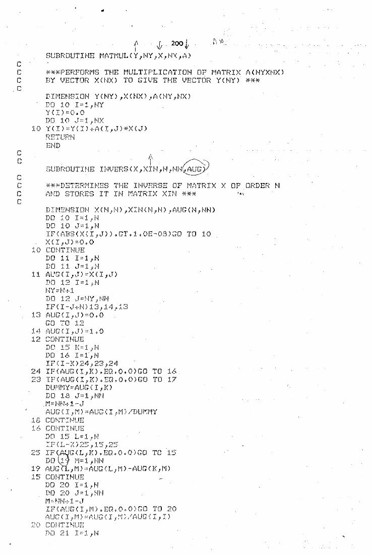
,[; 200 ~ SUBROUTINE MATMULCY 1 NY,X,NX 1 Al
c I"' J<··lH<PEm''DF!/'IS THE i'll.JJ.. 'l' I f"LI GAT I Di'l DF /'!ATF(I X A ( I·WX~IX l C BY VECTOR XCNXl TO GIVE THE VECTDR YCNYI *** c
,., '·'
c (., ·'
DIMENSION YCNYl 1 XCNXl!ACNY,NXl r•D :1.0 I" 1. 1 ~-IY Y(:::>===o.o DD :1.0 .. .T ::: t 1. !'IX
j.O YC:r>==Y(Il·t·A<ItJ)ifX(J) F~E7't.!!:::!\i
E-:!,!D
A~!D S1'DRES IT Il~ MATRIX XIN *** D!MSNSION XCN 1 Nl,XINCN 1 Nl 1 AUGCN 1 NNl DD :i.O I":i. ,.i-1 DD :!.0 ~.T=== :L 1 1>1 :[F(ABSCX(I 1 J)).G1".1.0E-03)G0 TO 10 X(I 1 \J)::(),.()
:!.0 CDJ··.fTINUH DO 11 I":l. ,~l DD :l.l IJ::::/.iN
11 A~GCI 1 Jl=XCI,Jl DD :!.~~.~ I===:L ?f\1 HY•==I···f+:l DD L'.~ ,.T=!-IY _, 1·-li'l IF<I-J-0N)13 1 14 1 13
:1. ::l :!Ol.JG C I , .. .ll '" 0, 0 GD ·~·o :!. ::;
:1. "·~ :'o UG ( I ,. ,J ) "' :1. , 0 :1. ;:>. CD 1·-!'l' :;: l•ll.J E
DD :J.:::; :(<=== :1. )N DD :1.6 I•"ltl'i IF' ( I··· I<) ~:.~4 1 1.~3 7 ~:~.c.!.
24 IFCAl.JGCI 1 Kl.EQ,O,OlGCl TD 16 28 IFCAl.JGCI,K),EQ,O,OlGCl TO 17
DU!'•'WJ'f:::f.,J..JG( I 1 1<> D Cl :1. 1:\ ,.r "' :1. t 1•11· I
.l1'!:::1·,JJ-.!+:J. "'tJ Al.JGCI 1 M)::ALJGCI,M)/DLJ~l'IY
:lD CCI!-.;T::PI..JE :!. 6 CD:··f'i' I I··IUE
:;: r· { L -· X< ) ::·.~ ~;:~ , :!. ~:; , ~? ~;): ;,:2:5 IF<~· G 0. ,ro, !::Cl. 0. 0) GO TO :15
DO :!. •: i''/::•:1. 1 1···11•1 1"? r!\UG ... ,1~) "t.:UG ( !..,1'1 l -AUG < 1< ,1.'1 l :!.5 CDI'·ITIHUE
DD ?0 :J>:I. ,H DD ?0 .J" 1 t !'li·f ,,, ::. f,/1,1··:<1. ·- J II·~(r~l...iG<I,I\'1) ~E(~,,o.~O)GD TD ;.~o
f~:UC ( J: !\'!) ::: f~1UG ·: J i :···: ~ .- 1 t"1UG ( :i: .t :;: )
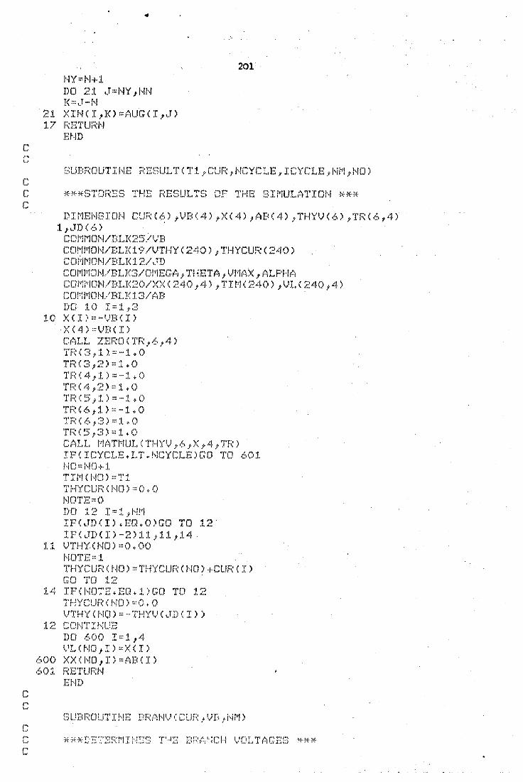
('' .•. , '·'
!'<':( " 1--1-LI. DO 2:1. ,,T=I,IY 1 !-IN l<'"<.T -·1,1
21 XINCI 1 K>=AlJGCI 1 ,J) :1.7 m:·:TUF(I-·1
Ef.Jl)
201
SUBROUTINE RSSULTCT1,CUR,NCYCLE,ICYCLE,NM 1 NOl c r ***STDRSS THE RESULTS OF THE SIMULATION *** c
c
'" '. ... c
DIMENSION Cl.JRC6l 1 VBC4l 1 XC4l 1 ABC4l 1 THYVC6l,TRC6,4l :1. 1 ,.Tl) ( (,, )
CDJ-rltv1Dl·-I/BLI<~?;:)/ 1,)B
COMMON/BLK19/VTHYC240l 1 1~YCURC240l CDi···lfYlDI,I/E~I .. I< :1. ?/ \.rD CDlvll~·iCJH./BI..X<~3/D!\'iE:G,t::; t THETf., 1 t..J!\'Jt:':iX 1 ,-::iX..PHr~~
CDMMON/BLK20/XXC240 1 4l 1 TIMC240l,VLC240 1 4l CC:H·:jf''I(J!·-f./BLI< :i. ~3/J-::In DD 10 I=:l. ,::l
:!. () XC I :• "-'.'El ( I l X ( 4 l '"VB (I) CALL ZEROCTR 1 6 1 4) Tl:~ C 3, :J. >. ::: ···:!. ~ 0 'fF:~ ( 3 1 :~) ::: :! .• 0 TF~<-4t:J.):::···:l. .. O TF;: ( 4 1 :;:. ) '" :1. , 0 TFt~ ( ~>, :J. ) ::: ···:!. <~- 0 TF: ( 6 1 l ) '"- :l , 0 ·~'P( 6 .t:;~) ::::1. (. 0 TF~ C !:>, 3) ::: :1. + 0 CALL. !~AT~llJl,(TJ·1YV,6 1 X 1 4 1 1'R) IPCICYCLE.LT.NCYCLElGO TO 601
TIIYJ(J··.fD) :::T:t THY cur:~ c i'ro) ::: o ~ o w:rn:: '" o DD :J. ::~ I~: :L i Hl"11 IF (,.IX) C I) • EO,()) GO TD l2 . IFCJDCil-2):1.1 1 11 1 14
:l.l VTHY,( 1,10 l '"0, 00 I·ICJTE,,:I. THYCURCNOl~THYCURCNDl+CURCil GO TO :!.~~
:L4 IF(!,!O~'E.EQ.1)G0 TO 12 Ti··!YCUr~ ( I"··!D) :::0 + 0 VTHYCNOl~-THYVCJD!Il)
:l? CDJ·-iTJHUE DD .-:;.oo I::: :t 1 4 \-'!. .. (1'-ID,I) :::)((I)
600 XX<NO,Il~ABCil 60:1. F::ETUF:I'I
El-f!)
c ,., '·'
202 DIMENSION CUR(6) 1 U8C4l 1 GMC6l,CBC4 1 6l 1 RBC4 1 4l,
:lXBUI 1 4l 1 t~BC4l 1 GBC4l 1 CBTC.6 1 4) 1 EJ•'I(6) 1 !':1(4) CONMON/BLK2/EM,B CCWII"IOIVBLK :1 ~'>l@' COMMON/BLK7/RB 1 XB 1 NB C~DI1'l!'K)/ ... J/DI..I( :f. ~3/ t~D CQ~;~!(J~I/BI.K5/CB 1 C;Br CALI~ I~A'i'MUI~<AB 1 4 1 CU1~ 1 J~!~,CB) ["I l ''" '!'1··•1 Jl cBo '1 [""·• JIJ•J· ... ,., ' ,; .. ) .•.• 111"1 '"· , 'd.t'' ,t l'i':t \ ,L ... :~, DD 10 l":l.t4 If :rr··:I---:;~):!.lr:l.:!.,:l.i.~ \
:1. :l VB < I l '" ... E < I ) GD TO :J.a
:J.<~ VB C:[) "'0, 0 :1.~5 DD :1.0 ~J::::J..t4
10 VBCil•VBCil+RBCI 1 Jl•AB(Jl+XBCI 1 J>•GB(J) CD!··IT I H1 .. a;: F<ETUF~H
E!'·lD
C )f**DE1'EF~~~I~!ES WHET}·!EF~ A~JY VOI .. TAGE OR C!JF~RE~!T
C DISCONTINtJITIES l·iAVE OCClJRED *~f~~
DIME~!E;ION CUR1(6) 1 CLJF~2(6) 1 ICI.C6> 1 VDC6>,VDDC6> 1 VBC4> 1 JD(6) COMMON/BLK8/VD 1 VDO c::l!''ll''IDJ·.J/DL!<61J·.ii..JI'I CDr~!rJDi'-1/DLI< 12/ .JD ~:; D 1·.-: l''l ~:J H / P ~-· K ~-:~:5 ./ vr:~ T\i,BO TI :::::~0
CALL BRA~IV<CLJR2 1 VB 1 ~1r!)
Cf~!I .. L Cf.JI'·!D (VB t \.JD) l)I)LJ]"•"] :1. ::: IJD ( !\!Ul'~"!)
\JDI .. JI''l2 '" t)!)CJ ( Hl...li'l) DD :57 I::: :L 1 b IFC\JDCI),LE.O.O>GO TO 37 IF<CVDUMl-VDCI)l,GE.O.OlGO TO 37 IPCICLCI),EQ,:J.lGO TO 37
'J'l):::TX JJ.:TV'" I
::;? CDIITI!·.J!.JE
IP<CUF~2CI),GT.O,Q)GCl TO ~~8
TX•CUR1CI)wSO/CCUR1Cil-CUR2Cill IP(1'X.G'f.1'I)G0 1'0 38 TI "'TX IJ·.JTI•I
IF(T'I tECJ,SO.Ai\!D~ TV.ECJ.!.1C>)G0 TO ·40 J·--12~=;.~
IP!TI.LT.TVlGO TO 41 I·!F':ITE ( ::. "::;oo l
'J.'E-::::T\J '•
(., .. c
c
I Cl., ( I i•IT\.') ":1. l··il'"l'"l··!i"'l+:!. l··i I. !I"' I " I H·T \.' GO TO 4:?.
4:1. ICLCJDCIN'I'Ill•O ~.II'(I TE ( :1. ,400)
203
400 PORMATC/:I.H 1 'CURRENT DISCON'> . n::"''I'I
i'il"'l• ~11"'1-· 1. GO TO 42
..:'.~() 1•1£.~::: :J.
DO 39 :!>:1. 1 1.'> ::J? vn:; c I > ·VD< I 1
F~ETUF:l··-1
El·.ll)
SUBROUTINE PLOTCNPTSl
C ***PLOTS VOLTAGE AND CUREENT WAVEFORMS *** c
,., '·'
c
C0Mil!ON/BL.K20/XXC240 1 4) 1 TIM(240),VL<240 1 4) CDr·W·iOIVBU<:J. '? /'.JTHY ( :>10) t THYCUF: ( :?.40) TLI!.,.!===O ~ G-400 RE10D ( !:5 _, ~~·) I'IDDE IPCMODE.2Q,:I.lCALL C!051N IF< 1\"iDDE. EO.:~) c,~,I.,L E:~3600
IFCMODE,EQ,3lCALL 95660 IPCMODE,EQ.41CALL T40:1.0 IFCMODE.EQ,41CALL UNITSC0.47) CALL DE\.'PAPC2:l.0.0 1 27'?.0 1 1) CM .• ! .. l.JTi•!I;CJ\d ( :?. ) c;,;u .. EI'<FWIAX ( :1. ())
C:ALL. c:~1AE;IZC1~5,2.5) Xl''!f~lX :::G. 0 TDTr-~,F~T:::TI/~'1(:!.)
l'i I HT~3 :::4 Xi'III·I"'O, 0
DD 0 IG::::J.,::~
DO 8 IPTS•:I. 1 NPTS IP<VLCIPTS,IGl.GT.X~!AX)XMAX=VLCI?1'S 1 IG> H'CVl .. ( IPT~3 1 IG) .l,'f .XI'IIHIXI'IH·l'"'-,!L( IPT:3,IGI
l:l COI,ITH·il.JE VYBEG•CFLOATCIFIX<XMIN/20.0))-1,01•20.0 VYENI>=<i~O·~FL(JATCIFIX(XMAX/20.0)))*20.0
IP<VYE~ID·tVYBEG>200 1 201 1202 200 VYEl~I>~-VYBEG
'')1\'::C .i,.\/ ,,·,.
GD TD ~::0:1. t,)YE{:c:G::: ···'JYEH:O CCN'l'IHUE CALL PENSELC1,0.0 1 0) CALL AXIPOS<:J. 1 45.0 1 233.0 1 60,() 1 1) CALL AXIPOSC:I. 1 45.0 1 203.0 1 60.0 1 2) CALL AXISCAI3 1 4 1 TS'l'ART 1 TLIM 1 1) CALL AXISCAC3 1 NINTS 1 VYBEG 1 VYEND 1 2) CALL AXIDRA<2 1 1 1 1l
..
'•
CAl~L AXI)RA(-·2 1 -1 1 2) DD·;:-- IG,,:I.,,::J D(J 1.0 :EI~T~~:=1 1 1~F·T~3
10 VLCIPTS 1 :1.l=VLCIPTS 1 IGl JF''EI'i'"IG+:I. CALL PENSELCIPEN 1 0.0 1 0l CALL GRAPOLCTIM 1 VL 1 NPTSl
9 Cm·ITI!·II.JH c C *** PLOTS LINE CURRENTS *** c
XI"' I I 1·1 '" 0, 0 XI•·!,~,)( "' 0. 0 DD 1.1 Il> :L 1 :.:;
DO 11 IPTS=1 1 NPTS IF<XX<IP1'S 1 IG>vG1'.XMAX)XMAX~XX<IF~TS 1 I(;) IFCXXCIPTS 1 IGl.LT.XMINlXMIN=/XCIPTS,IGl
1 :1. cmrn: r·IUE VYBEG=CFLDATCIFIXIXMIN/20.0ll-1,0l•20,0 VYEND=I1.0+PLOATCIFIXCXMAX/20.0lll•20.0 IPCVYEND+VYPEGl203 1 204 1 205
<~03 VYE:I··il) '" ... VYBEG GD TCl :?.04
20~5 VYBEG :::OH tJYEND ~.~04 CC:1-ITIHUr:
CALL PENSELI:l,O,O,Ol C:ALL AXIF·!JSC1 1 :L25.<> 1 2:~8.0 1 60.0 1 1) CALL AXIPOSI1 1 125,0 1 203.0 1 60.0 1 2l CALL AXISCAC3 1 4 1 TSTART 1 TLIM,1l C1~LL f'oXI~3Cf'o ( 3 1 HIHT~3 1 VYX:<EG 1 'v'YEHD ,:a) CALL AXIDRAI2 1 1 1 :1.l CALL AXIDRA<-2 1 -1 1 2) DD 1~.~ IG::::J.,:~
DD 13 IPTS=l,M~Ts 18 XXCIPTS 1 1):=XXCIF'TS 1 IG)
IPEH'" IG+:I. CALL PENSELIIPEN,O.O,Ol CPoLL GPtoF'CJL C TII'i 1 XX J·IPTS)
C *** LABELLING *** c
CALL MDVT02C45.0 1 266.0) CALL PE!~SEL(2 1 0.0 1 0) CALL CHAHOLI'VBC:I.l,•,·l CALL PENSELC3 10,0 1 0l CALL CHAHCJLC'VBC2l 1•,·l CALL PEHSELC4 10.0 1 0l CALL CHAHCJLC'V8(3)•,"l CALL PEHSELC1 10,0 1 0l CALL CHN·IOL (. C \.'"·LDL'l'D) "',. ) CALL MOVT02C125t0 1 266~0) CALl. PE~ISEL<2 1 0.0 1 0) t:Al.L C!-!A~1(:~L(~CURC1),~~.')
CALL PEHDBLC3 1 0,0 1 0l CALL CHAHOLC'CURC2l 1 •,")
CALL PENSELC4,0,0 1 0) CALL CHAHOLC'CURC3l•,'l CALL PEHSELI1 10,0 1 0l CALL CHAHCJLI' <A•LMPSl*,") CALL MOVT02Cl06,0 1 233.0l
..
c
CALL PENSELCl,O.O,Ol CA I.. I.. CHt-d··IOL ( I ( f:' )1~ I .. EC~:~) V· ~ ' )
CALL MOVT02C186~0 1 233~0) CALL CHAHOLC" <S•LECSl•."l CALL MOVT02C45.0 1 198.0l CALL CHAHOLC"FIG 4.10•UA, •UPHASE VOLTAGES*,") CALL MOVT02C125.0 1 198.0l CALL CHAHOLC"FIG 4,10•UB, •ULINE CURRENTS•,")
C *** PLOTS THYRISTOR VOLTAGE *** c
XI"1Ii··i"O, 0 Xl'"lt•X"O. 0 DO 14 IPTS•1 1 NPTS IF ( VTHY ( I PT~:; l , GT, Xl'!.tc,X) Xl'IAX '" VTHY C I PT~3 ). IPCVTHYCIPTSl,L'I',XMINlXMIN•VTHYCIPTSl
14 COHTII·IUE VYBEG=CFLOATCIFIXCXMIN/20.0ll-1.0lW20.0 VYEND=(1,0+FLDATCIFIXCXMAX/20o0lll•20,0 IPCVYEND+VYBEGl209 1 210 1 211
20? VYJ:!l'.fD"' ·- VYDEG GO TO 210
;.~:l:l VYXJEG= ·-VYX-:J,ID 210 CALL AXIPOSC1 1 45.0 1 157,0 1 60,0 1 1l
CAl .. L AXIF'OS<1,45.0,127o0,60.0,2) CALL AXISCAC8 1 4,1'!31'ART,TLIM 1 1) CALL AXISCAC3 1 HINTS 1 VYBEG 1 VYEND 1 2l CALL AXIDRAC2 1 1 1 1l CALL AXIDRAC-2 1 -1 1 2) CALL GRAPOLCTIM 1 VTHY 1 NPTSl
c C *** PLOTS THYRISTOR CURRENT *** C'
XI'"!.'\X =0. 0 DO 15 IPTS•1 1 NPTS IPCTHYCURCIPTSJ,GT.XMAXlXMAX•THYCURCIPTSl IFCTHYCURCIPTSl.LToXMINlXMIN•THYCURCIPTSl
:f. ~:5 CD I .. ! 'I' II-.JU!:~ VYDEG=CPLOATCIPIXCXNIN/20.0))-l,OlW20.0 VYEND=Cl.O+PLOATCIPIXCXMAX/20.0)ll•20.0 IPCVYEND+VYBEGl212 1 213 1 214
~21.:?. 1..}'{};:/,iD::: ···'v'YB.r:G •: GD TO 2-~:l.a
214 VYBEG=-VYEND 213 CALL AXIPOSC1 1 125.0 1 157.0 1 60.0 1 1l
CALL AXIPOS<1 1 125.0 1 127+0 1 60~0 1 2) C'~JI Av·r~cAc~ A 'J'~-Af'~ ·L·r~l '> · .~t··t ..• .•.. ,,,,_), .. · .. ~,'I .. ).~t··t \.1. 1-~ . It·'·
CALL AXISCAC3 1 NINTS 1 VYBEG 1 VYEND 1 2) CAI~L AXIDRAC2 1 1 1 1> CALL AXIDJ~AC-2,-:L 1 2) CALL GRAPOLCTIM,THYCUR 1 NPTSl
C i~*~' PLOTS DIODE VOLTAGE AI~D·CUF~RE~ITS *~~~~ c
CALL MOVTD2C45.0 1 18?.0l Cr~,r..r.. CHr~d··IDL ( 'VD I CJilE C V'•(· LDL TS) ,,; , " ) CALL MOVT02C125o0 1 18?,()) CALL CHAHOLC"DIDDE CURRENT CAwl..MPS)w,") CALL PmVT02(106o0 1 157,())
c
(" ..
..
CALL CHAHOL(' <S•LECS)M,') CALL MOVT02C186.0 1 157.0) CALL CHAHOL(' CS•LECS)M,') CALL M{JVT02C45~<> 1 122~0)
206
CALL CHA~OLC'FIG 4.10•UC. •UVOLTAGE ACROSS DIODE 1M,'l CALL MOVT02(125.0,122.0) CALL CHAHOI.C'FIG 4.10•UD, •UDIODE CURRENTC1)M,')
:.<:,·:~;;x ::: o. o DO 16 IPTS==1 1 NPTS IFCVLCIPTS 1 4l.GT.XMAXlXMAX=VLCIPTS 1 4l
:l6 CDHTIJ-..JUE VYBEG=O,O VYEND=C1o0+PLOATCIPIXCXMAX/20.0)))M20.0 NINTS•IFIXC-CVYBEG-VYENDl/20,()) CALl. AXIF)OS(1 1 45.0 1 51.0 1 60.0 1 1> CALL AXIPOSC1 145~0 1 51.0 1 60.0 1 2) CALL AXISCAC3 1 4 1 TSTART 1 TLIM 1 1l c;,~LL i~)<JGCti C 3 1 1'-ii1",:T~3 1 \}YJ:-!EG 1 '·,.JYE!··ID ,:~~) CALL AXIDRAC2 1 1 1 1) CAI .. L AX:[DF~A<·-2 1 -1 1 2> DO 17 IF~!S=1 1 ~!F'1'S
17 VL.~IPTS 1 1>==VLCIF'TS 1 4) CALL GRAPOLCTIM 1 VL 1 NPTSl
IFCXXCII:)TS 1 4).G1'.XI1AX>XI~AX=XXCIJ~TS 1 4) 113 CDNTINUE
VYE~!D~<1.00·FL(JATCIFIX(XI1AX/20.0>>>*20.0
CALL AXIPOSC1 1 125.0 1 51.0 1 60.0 1 1l !:Al .. L. AXIF'OSC1 1 12~~.<> 1 5~.0 1 60.0 1 2) CALL AXISCAC3 1 4 1 TSTART 1 TLIJ~ 1 1) ~!II\ITS=IPIX<VYEND/10.0) CALl~ AXISCAC3 1 NINT~3 1 VYBEG 1 VYE~iD 1 2) CALL AXIDRAC2 1 1 1 1) CALL AXIDRAC-2 1 -1 1 2) DO 19 IPTS•1 1 NPTS
19 XXCIPTS 1 1l=XXCIPTS 1 4l CALL GRAPOLCTIM 1 XX,NPTSl CALL MOV1D2145.0 1 113.0) CALL CHAHOLC'VB(4) CVwLOLTS)M,') CALL MOVT02Cl25.0 1 113,()) CALL C~1AI~Ol.('CLJ!:~(4) (Ai(L,MPS>~~.')
CALL l~OVT02C45.0 1 36.0) C~~LI .. CH~~~HDI.. \'FIG 4 .. :1.0·)(·/.JE • ·!O:·ULC:f.iD \)DL'I'(.:lGE ¥.·.' )
CA!.!~ !10VT02C125.0 1 36,0) CAI .. L (~~1A~iOLC'FIG 4.10~~lJF. ~fl.Jl.CJAI> CLJRF~ENT 1f.')
CALL MOVT02C106f0 1 51.0) CALL CHAHOLC' CS•LBCSlM,') CALL MOVT02C1<36.0 151.0l CA!..!.. CHPd··!CL C ' C >>:·I.J:·:C':l) >(·, ' ) CALL MOVT02C46.0 1 2S,O> CALL CHAHDLC'FIG 4o10•UWAVEFORMS OF A PASSIVE LOADM,') CALL CHAHOI..C' FED PROM THE BUSBARS BY A SMALL LENGTH•,') CALL MClVT02(46.0 1 20.0) C:Al.L c:~·JA~·Il~Id(' 8F C~ABLE,~·~·IF~OlJG~i A~~ F'~·IASE D:!:DDE BRJ:I)GB~~.')
/ ("' ,, c c c ("
c '" ,, ,., ~
("
..
207
****~f**~~**~&**~f~~**~&**~&if~¥if*~f*~f~fi~iG~f*~~~fif*~f***~f****~f**~f*if~~if~fif~f
~f~~~ SIML!: .. ATIO~ OF A l~ASSIVE LOAD FED FRO/~ Tl·~E BUSDA~S ~~*~!
*~f* BY A ~~MALL. I~ENG1'~~ OF CABLE 1'!·~~~0LJG~i A 3 p~;ASE FULLY ~&*~f *** CON1'ROL~ED TH\'RIS!'OR BRIDGE F'OR ANY TI~JGGEI~ Al~GL.B ~~f:l~ *****~f*~f**~f*~f**~fifif*~f~f~f*if~fif*if**~~***if*ifif*~f~~ifif~f**~~f~f~f*if***~f**
DIMENS;I8N CBRAN<4 16) 1 EMC6) 1 E(4)jCtJR(6) 1 f~BC4) 1 XBC4) COMMON/BLK20/XXC400 1 4l~TIMC4001 1 VLC400 1 4) COMMON/BLK19/VTHYC400l 1 THYCURC400) CCJI\'/!•·:DJ··.J/BLI<::::;7 /l···i'I'f~ I G, N~:;TEP .t 1·-.JCYCLE
CD:-1:l 1'lDI·~f/Tn .. I<7 /nB 1 XB £:
(~0MJrJQN/BLK1/CBRA~I
CDt···!f'"!D!~-J./E~Ll<~?../~:~1\'i i E CCi~~!Cl!,I/BLK3/0~lEGA 1 T!"!E1'A 1 V~!AX,ALf:·!·1A C(JI11~0!~/BLK4/1~(4) 1 GC·4> 1 TT(4)
C ~~~&*RE~;ns INITIAl. DATA ~~~G*
c
c ,., '··' c
c
"'•"''('[) ~~. ) !'""• 'l'! 'I' I'' I"O...l".', •• , • -~l ~(· ... !'',. }' •••• ,
r~r;:l;D ( 5 t ~~(·) J··.JCYCLE F~EAD(5 1 ~~)(RBCI> 1 I~1 1 4) I~EAD(5 1 *)(XBCI> 1 I::1 1 4) t.) !''/ f~l X.::: 12 0 ~ 0 ~(· ( 2 t 0 ·)(· ·)(· () t' ~> ) / ( ~~ -) 0 ·)(· ·)(· () i> ~;;; )
SQ:;:(~5t0/f,0)¥10.0~f~~(-4)
F'I :::4 • 0·)\:AT(.,J-..! ( .1. -~ ()) [!h·!EGt! ::: ~:, ()~~.:·F' :r ;li·Ff(
THETt1 :::7.: ~ O·)(·F'I /3, 0
CALL ZEROCCBRAN 1 4 1 6)
C *** SETS CONSTANTS PDR INTEGRATION ***
c ,., L,
c
H ( 1. ) ::: :1. • 0/::~. 0
H\c:·l"'l,O H(4)'"C',() G ( :!. ! ::: ::. ., (J/ 1..~ • 0 G (?) ::: :L. 0/:~ ,. 0 G ( :3) '":!. , 0/::J, 0 G ( 4) ::: :t ~ 0/6. 0 TT<:J.):::OvO TT 0: ;,~) '" :l , o;;:' , () TT<:~~)::: 1. t' 0/~?-) 0 TT C'-i I " :l , 0
cr·:·:r;:td"i ;~ :~. ,t ::. > ::: 1 ., ::> CE:F:(:JH ( 1 I::_::) ::: :l (· 0
..
CE<f(('ol··l < :1. 1 4 l '" -· :1 .• 0 CI<f(r~H ( :l , :'i) '" ·- :l , 0 Cl':I'(AI'I ( ;.~ ·' :1. ) "··· :1. • () CE:F'..:,~~H ( ~:~ 1 ~3) ::: :1. • 0 cr:Fr.,; .. ; < :'!, 4 l "' :! .• o CE:r~r~,J\1 < 2, .·s) ::: ···-:!. "o CDF~(.,J-..J ( :;~ .t 2! :;: ··· :!. t 0 CE::F<(~,J ... J ( ::; J· :::.) ::: ... :!. ~ 0 ~:;.r.::F\'Pd.,l ( ::~ .t:;:) ::: .t,. 0 CBI":r~~IC:');-/·,) '":1. .0 DD -40 :::;:: :1. .t ,(.,
40 CBRANC4 1 I>~1,.0
20B
C . ~~** SETS :rl~ITIAL MES~1 Ct.JF~RENTS A~ID 1'f~IGGER ANGl.E 1~** DD lOO I c<l t 'I HTF~IG"' ( I···:l. )lf:I.O T:i."O.O
cur:~< J-iJ··!) ::: o ,. ooo :L c C *"* SSTS A PAIF OF T~YFISTORS FOR CONDUCTION INII'IALLY *** c
("'
C *~~* COMF~LJ1'A'I'I(J~I BEGJ:~:S *** c
r·
CAL.L·RlJNGE(1'1,N~!,ClJF~ 1 SO,XX,Vl.,V1'~1Y 1 THYCUR 1 TIM>
Cr~,LL Y.:.:XIT Ei'-iD
C *** ~iETS INITIAL LOOP AND I~IF'EDANCE ~!A1'RICES ~~~* I' '·-·
,., '" ,., '·'
c
DIMENSION VD(6l 1 VD0(6l 1 VB<4l 1 ICGNDC2l 1 E<4l 1 EM<6l CDl\'//''iO!···!/E~L}(;;:::~;}/ 1·)B
COMMON/BLK27/NTRIG 1 NSTEP,NCYCLE CO~MON/BLK8/VD,VDO
COMMON/BLK:I.2/ICOND C Cl!"-"il'"l CJ H/13! .. IGYF:i'i , H DD e. 1> :l ,2
I:\ ICOI,ID (I)"'()
CM..!., Ei"'IF ('X' :1. ) DC :to :1::«:1_,.4
:i.O 'v'J:<( :;: ) '"E< I)
DD :J.4 :J::==l_;./' :i 4 VDD ( I) ::: 1-)D ( ::: )
IF(~ITRIG.I~E.40)1CDND(1)=6
IFCHTRIG.GT.40liCOND<ll•5 CALl .. TF:AI,!::H·'I ( 1•1!'1) l:~r:Tur::l'·' x:-:;,1!)
~3LJBRO~.J1'I!~S 1'RANS~!(NM)
C *** FD~MS TfiE TRA~iSFDRMATICN ~!ATRICES DEPENDING OH THE (~ Al::·f::·ROPRIA'I'E l~(:l()F' CONDlJCT:l:I~G ~~~~*
(. -
c c
c
c
r c
c
209
DIMENSION CBC4 1 2l 1 CBTC2 1 4l 1 CBRANC4 1 6l 1 ICONDC2l COMMON/BLKl/CBRAN COMMON/BLK5/CB 1 CBT COMMON/BLK12/ICCND CALL ZERO<CB 1 4 1 2) CALL ZEROCCBT 1 2 1 4) J:FCl~~l~EQ,O)GO 1'0 11 K=1 DD 10 I=1 1 NM Il=ICOI~D<Il DO lS J=1 1 4 CBCJ 1 Kl=CBRANCJ 1 11l
18 CBT<K,Jl=CBRANCJ,Ill K=K+l
10 CONTINUE 11 RETURN
END
S~lJB~C~~JTI~!E I~!F'(ZB 1 ZM>
DIMENSJ:ON ZB(4) 1 ZM<2 1 2> 1 CB(4 1 2) 1 CBT<2 1 4) 1 1 ZTC4 1 2l COMMOI~/BL~S/C:B,CBT
CALL ZEROCZT 1 4 1 2) DO l.O J=1 1 2 DO .10 1=1 1 4
10 Z1'CJ:,J~=ZB<I>~~CB<I,J) CALL MAT!~PCZ!1 1 CBT 1 ZT 1 2 1 4 1 2) RETURN E~
SUBROUTINE MATMPCA 1 B1 C1 L1 M,Nl
C *** PERFORMS THE MULTIPLICATION OF THE MATRICES BCL 1 Ml C AND C<M 1 Nl AND STORES IT IN ACL,Nl *** r
c c
c
DIMENSION A<L 1 Nl 1 B<L,Ml 1 CCM 1 Nl DO 10 I=1 1 L DD 10 J=l,N A!I,~!>=O,O
DO 20 K=l,M 20 A<I,~J)::A<I 1 J).~B<:C,K)*CCK 1 ~J>
10 CONT:l:l~WE
RETURN E~ID
SUBROUTINE CONDCVDl
C •••DETERMINES THE VOLTAGE ACROSS EACH DP THE THYRISTORS *** r
("
c
VDC3l=UBC2l-VBC3l+VBC4l VDC4l•VBC2l-VBCll+VBC4) VDC5l=VBC31-VBCll+VBC4l VDC6l=VBC3l-VBC2)+VBC41
EHD
210
E:~UPF'DUT .THE-; D I t)C()f,l ( CUF.':I. 1 C.~UF:.~? j· ·:·1~, 1·-1.::~; S j h'i'•'/ 7 h'F .:- ! ... !T 1 I CYCLE) c r ~~*i~C~1ECKS FOF~ BCT!-~ VOl.T~GE ANI) CU?~f~ENT !>ISCO~!TINUITIES **~• f''
'" D!MEHSIOH CUR1C6l 1 CUR2C6l 1 NTC2l,VBC4l~VDC6Y 1U~OC6l,TINTC2l 1 1 AIC6l 1 ICONDC2l
COMMON/BLK12/ICOND CDMMON/BLK8/VD 1 VDO CD I''! 1.,.! D f-~ / B L I<~-~:::; I \.JkJ
TI!,!T( l) :::f:3
TIJ·,JT < ~~) :::~3 C *~~* C~iECXS FOF~ A~!Y CLJf~RENT DISCD~lTI~!UI1'Y ~~~~~~
IFCNM.EQ,OlGO TO 11
c
c
DD 1 0 J>:l. , 1··11'1 IPCCUR2Cil,GT.O.OlGO TO 10 TINTC1l=CCUR1Cil•Sl/CCUR1Cil-CUR2Cill nrn:=I
.l. 0 CDHT I !'1\.JE
CALL BRANVCCUR2 1 VB 1 NM) ::;,o, LI.. CD I'!D < \!J) l IFCNF,EQ,O)GO TO 30 DD :;:: :!. 1< ::: :J. 1 !···iF·'
J:F<VDCNO)tLE.C>.O>GO 1'0 21 TVOL=-CVDOCNOl•Sl/CVDCNOl-VDD<NOll IFCTINTC2l.LT.TVDLIGD TO 21 TIHTC/.c) "T\lC!L HITV,,!,IO
21 COHTII,iUE C ~~~~~~ C~ECKS FOF~ M:rN:rMUM TIMB OF DISCONTINtJITY ~f*~f*
30 :EF(!It~T<2).EQ.S.AND.'riGIT<1>.EQ.S)G0 TO 220
c
1···!~?:::2
IF(TIN1'C:L>.L1'.1'IN1'C2>>GCl TO 215 T.t:-::::TII··-I'F < ~?) DD ;,;_~:;-~ :!:::::J. .~i--il.,.l
22 AI<Il=CCCUR2Cil•TINTC2l)+(CUR1CilM(S-TINTC2l)l)/S
C *** IMPLIES \lDLTAGE DISCONTINUITY *** c
IFCNMPR.GT.OlCURlCNMPRl=AICN~PR) I··.J n::· F;: " J·,i F !··lT':::!··!F'···l 1··-lT.:: :1.) ==-/·.;'!:' ( ~--!F'F·F~) NT (:'I!" PI'!) "' ()
(., ,,
c
c c c
G c
..
211 I CC)!,:!) C 1>11'1 l "li·,ITV GO 1'0 ::.'1.6
215 DO 217 Ia1,NM 217 AICil•CCCUR2Cil*TINTClll+(CUR1Cil•CS-TINTC1llll/S
cur;~ :I. ( If-..JTI) ==o o o I CD!'-1)) ( :U·!'r:l: ) '' 0 :i:F ( ''·W: C· X::.'Q. ())GO TD 2.1. _f.,
CUR1CNMl~AICNMPRl
cu;::: :1. c r--:!'IPF: l "o. o ICONI,(l)==ICO~ID(~I~/PR>
ICDI·-!D < 1--i!'"ll::'i':) ,,0 2:1.6 CDI··I'l':J:I,IUE
c,-.~u. 'IT',~"'':::''' c ~11·1 > f(ETUf::!'l
:~~~() t·.J::~ ::: 1 Tit:::S F\ETUF::i'·l ;::~m
SUBROUTINE ZERDCA,N,Ml
l>Ii"II:I·-Im:C.li',l ~~ ( N ,!.'1 l no 1 o :r ,, :l , ,,, \)(} 10 ,,!,, 1 t~'-~
1 () ,<\ C..l'; J) a(),()
F:ETl.Jf::l·l Et·ID
SUDROl.lTINE EMFCTl
' A ' r··i
r ***DETERMii~ES THE IMPRESSED VOLTAGES IN EACH OP THE C BRANC~iES AND I~ENCE THE MES!·iES *** c
c
c
DIMENSION EC4l 1 EMC6l 1 CBC4 1 2l,CBTC2 1 4l COJ~MON/BLK~5/CB 1 CBT . COMMOH/BLK3/DMBGA 1 THBTA 1 VMAX,ALPHA COI'II'•'ID/·-1/ro.J.JC:iUE!''/ 1 E ECll•VMAX•SINCOMEGA*T+ALPHAl E(2)=VMAX*SIN<OI1EGA*T-THBTA·0ALF'~iA)
EC3l•VMAX•SIN(DMEGA*1'+THETA+ALPHAl
CALL MATMULCEM 1 2 1 B1 4 1 CBTl F:ETUF:.:i·i E/>/1)
SUBRO~TINE RUNGECT1 1 HM,CUR,S0 1 XX,VL,VTHY,THYCUR 1 TIM)
(~ ~~*~G C:O~JF·tJ1'A1'IO~! CARRIED [JLJ1' ~~~~i~
c DIMS~ISION CUR1C6l,CUR2C6l 1CURC6l 1 VBC4)
1 11Jl)C6> 1 VDOC6) 1 J:COI\!D(2) 1 Y!1(2 1 2) 1 !\!1'C2)
212
COMMON/BLK27/NTRIG,NSTEP 1 NCYCLE CD/"//''/Dt-//BLK2~')/!JJ3
COMMON/BLK12/ICOND C 0 l''ii''/CI NIB LW?/'!'!.. I /'/ :·.JEi<T '" :1. +I CDHD ( H:··J) IP<NEXT.GT.6lNEXT=NEXT-6
\JJ:::O DO 21() IC;YCL.E:=1 1 ~!CYCI .. E
DO ?:1.0 ITHY===l,c-6 DO :l99 IK~:L,~ISTEP t·.JO" /·.JEXT IPCHO.EQ,6.AND,ITHY.GT.2lGO TO 2006 IPCNO.EQ,:J.,AND.ITHY.GT.5lGO 1U 2005 IFCNO.GE.6lHO=N0-6 GO 'I'D 2006
200.1., I:L===ITHY·-HD IPCiloLT.OlGO TO :1.19 1\!X'I'£~!-,JG::: II<+ ( J :l. ·H·H~:;Tr:P) IP<NTRIGc.LEc.~IX1'A~!G)G0 TO 2002 GD TO :i.:l?
2002 IF<VD<~·!BX1').GT.Oc.O>GO TO 2003 J·.JF=J·.JF+:I. !·>f'T =: l'IF) ::: 1\IEXT J··!EXT::: J··.JEXT+:l IF<NEXTc.G1'.6)NEXT=~IEXT-6
GD TO :i.:l.~"'-~
:'.' () () ::l f·l!'!i"' !':: "' J·.J !'/ IF ( t·IF " EC~ • 0 ) GO TO ~~0 :!. 0 J•!Fr''f.:: '" :·.JF J··!F,,J·.JF ... :l :·.JT ( :1.) =t·i~' ( ~IF'PF:: l ~IT ( HFF'I'O '"0
c:ur::: < ~·ll"l; "'o, O<'O:I. I CD1··.JD ( Hi1!) ::: i"iE·:XT J·.JEXT '"HEX'!'+ :l IF(~IEXT.G1'.6)NEXT=NEX1'-6
CALL TF\(o/··1~3/'·1 ( ~WI l 1:1.9 IFCNM,EQ,()lGO TO 101
DO 20 I(<l 1 !·1/"1 20 CUR1(Kl=CURCKl
:I.O:l ~3:::f)0
C:ALL RK4CS 1 1'1 1 CLJR1 1 CUR2,~1M 1 Y!'f)
:300 C(.!~:. .. r.. D I ~::CD!··l ( (:;ur;: :L l CUF~:=.~ 1 Tl''i J J···l 1 Hi?. .t ~;) 1 J··il''l J !··IF 1 1··.f'I' 1 I CYCLE) IT:·~ i'.J:,:.~ + ::~0., :l. ) GD TD ?3~:;;
Ct~:LL CDHD ( \)D} T:L :::"f.':l. +T~''II!···l DO :?40 I= :1. tC'
::'40 VDD (I) '"'-'D (I l ~;) =~ ~;; ·~ T !''I I N CALL RK4CS,T1,CUR:J. 1 CUR2,NM 1 YMl DD •.;;"? I= 1. 1 J.J/'J
99 C!.JRCI>=CUf~2C:r>
GO TCl ::lOO 235 !)0 242 I~1,~111 ?l~.:~ cur:: (I) :::CLJF:? (I)
:ern ~.~41 I==: :J. /f.·,
..
213 'I'1 :::Tl+~) CALL RESULTCT1 1 CUR 1 JJ 1 NM 1 ICDND 1 XX 1 TIM 1 VL,VTHY 1 THYCUR 1
liCYCLEI . :L '1'? CDNTII··IUE ;::10 CCH'·ITII,IUE
CM .. I.. F'LOT < ,,l,.T, Tc .. I/'1 ,Xi<_. TIM ,VI.. ,VTHY 1 THYCL.If~ I
EHD c (" ,,
c C *~~~~~~tJNGE-KU1'TA POUF~TH DRDEF~ I~iTEGRATION IS F'ERFORMED ~** c
r c
c
DIMENSION CUR1C6l 1 Cl.I~2C6l 1 CURDUMC61 1 Cl.IRDELC61 1 CURDERC61 :l 1 RMC2 1 21 1 YMCNM 1 NMl,EMC61 1 VC61,GMC6l 1 EC41 2 1 XMC2 1 2> 1 RBC4) 1 XBC4-> 1 AUGC2 1 4Y C(J!~MO!~/E:LK11/RI1 1 XM ~~
CDMMDN/BLK 4/HC4l 1 GC41 1 TTC4l CDMMON/BI..K2/EM 1 E CGl.,ll"iCi·-.J/I~LI< :J. ~;;_./Gl .. ! COM!10N/PLK7/RB 1 XB Ct;LL I !·•!F" (m:-:, l'<i"l) C{:J~I.. :r. r···:p c x:e 7 X!YJ > I?CNM.EQ,OlGO 1'0 60 i'l /'.! " 1··11'/ '•(· ::!. CALL INVERSCXM,YM 1 NM,NN 1 AUGl DD l 0 !( "'l f ~·liY/ CUF;~DUiv! ( !() ::: Ct..u:;~ :I. (I<)
10 Cl.IRDEI..CKl=O.O 60 !){) ~-~o ::: :::~uH ::: :1. , -4
T2==1'1+TT<IRU/~)*S
C/:iL!.. E:J·rlr' ( T;t.~) IPCNM.EQ,OlGO TO 20 CJii .. L Cl.HWDT C Ct.Jc::!:•t.il"/.,. CUF:o)EF:;, I'll''!,- Yl''l; F:i''l l DD ~;;;() T< ::: :L t 1-!!''l CU~~DEL<K>~CtJRDELCK)4-GCIRtJ~I)ifClJ~~DEF~CI<>~~s
:2.0 CUFWi..Jl'l C !0 .,. CUFn (I<).; H ( I F:l.J/'1) ,~-cJ.JI'm:t:F<e I<) ''fS :?O CDi·iT I 1,/UJ:.:
IFCNM.EQ,OlGO TO 61 l) 0 4 0 I< "' :1. 1 i··/1'1
40 CUR2CKl=CUR1CKI+CURDELCK) CALL MATMULCV,NM,CUR2 1 NM,RMl DD ~'}() I "' 1 ,.. Hi''/
SUBROUTINE CURDOTCCUR 1 CURDER 1 NM,YM 1 RESl
C ***OBTAINS THE DERIVATIVE OF THE MESH CURRENTS *** c
Dii'1IEHBIDN CUP(6) 1 CUi:~DEH(6) tEftl(tf.,) tF:~EB<J-.J!vllNl''l) .t
1YMCNM 1 NMI 1 VDROPC6l 1 EC4l CDJYJ/'•'!C)J···i.-'B1 .. :~<? .... E/YJ -~ E CA! .. L tr1ATI~Ul,(VD!~~()P,!·-:M}Ct.JR,NM,RES) D 0 :1. <> I "' .!. ,, 1···11·•; tJDf~()!~<l:)::EM(I)- 1JD!~O!:~<l:)
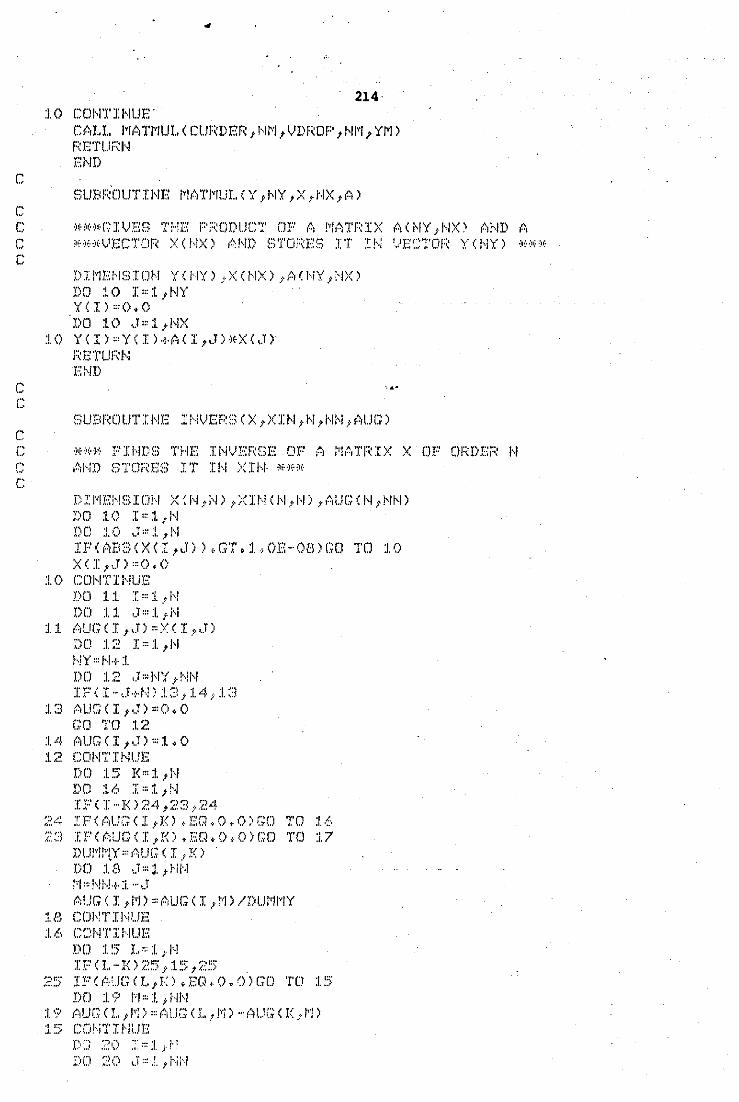
c
c c
c
c
214 :1. o c o l'rr :n 11 .. 1 r: ·
C~.I . .I.. I•IATI'IUI .• ( CUI'\l>I-m 1 !,1~·1 t VDFWF'' t !'11'1 1 Yl'l l FmTUf<H EI'ID
SUBRDUTIHB MATMULCY 1 HY,X,NX 1 Al
***~IVES THE PRODUCT OF A MATRIX ACNY 1 NX' AND A il\·~~~:··)l·VECTDF~ X ( l,tX) (~HD ~:>TOF~E:::; JT I!'·i 1)EC'~'OF( Y ( 1\iY) ·)i··)(··)(·
D I l'~'!El··!!:3 T Dl'·i Y ( 1··./Y.) }-X ( 1'·1><) t ;~ ( J··.tY 1 l'IX) DD :LO l"':l 1 HY YCil,,O,O DO 10 ~.T ::: :l }·!'-!X
10 YCI>~YCil+A<I,J)MX(J) F~ETUF\N Ec,iD
SUBRDUTIHE INVERSCX,XIN,N 1 NN,AUG)
C *** FINDS THE INVERSE DF A MATRIX X OF ORDER N C AI~D STORES IT IN XIU ~~~~~f
c DI~!EJ~!SIO~I X~N,~I) 1 XINC~I 1 1,1) 1 AUGCN 1 NN) DO :1.0 I::: :1. i ! ... J
DD J.O \,r::::!. ,l.,l IF<AB3CXCI 1 J))tGT~1~0B-08)(;Q TO 10 XCI,\J):::OvO
:!.0 CDNTii··!UE DD :1.1 I===:i..tf'! DD :l.l ,J,":I.ii'i
l:l AUGCI 1 Jl=XCI 1 Jl D () :t::> I = :1. t 1··1 i···!Y'"~'-~+:1.
DD :12 ,J=I··IY 1 J·.iJ··I IF<I··~J+N)13 1 14 1 1~J
:t::l ,o,u(;;c I , • .r> =o.o GO TO :t.~?.
:1.4 A UG < I 1 ,.T) '" l , 0 :1.;" CDHTI!-II..!E
D D :l ;;; I< '" 1. _, f··l DD :l6 I::::l. 1 1'·1 IF( I···!<)t.~4 ,::~~~l~i.~4
2~ !PCAUG<I,Kl.EQ,O,OlGD TO 16 23 IF<AUGCI,Kl.EQ,(),())GO TO 17
DU!···Jl'fx' ::: (\!.JG < I t I<) D 0 1.1:"~ ,.1 "' J. t l··iJ·.J :·rj:::!,!H+:i. "'t.T AUGCI,Ml=AUGCI 1 Ml/DUMMY
:i./:1 CDI-~TI!-ii.JE
DD :15 l .. " :1. , 1··1 IF-' ( 1.. ... I<);;_:::::; .r :1. ~> t i.:~::;
25 IFCA~G<L,Kl,EQ.O.OlGD TO :1.5 DD :1.? 1"'1 "' :1. , 1··11'1
19 AUGCI~,J~)=AlJGCL 1 /~)-AlJG(!( 1 M) :J. ~;; CD!···i'X' I !··lUE
D :::; :? ~:> :;: ::: :!. }- 1· t DD :;~ 0 \.T ::: :L 1 i···i i··.J
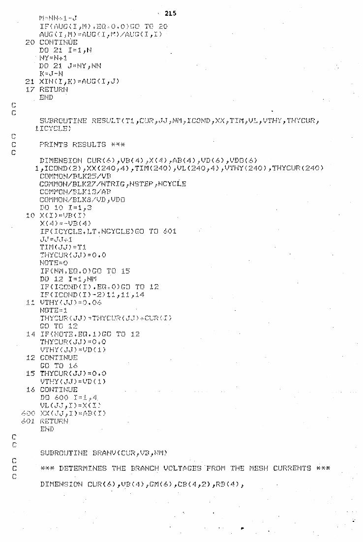
c
' 215
IF<AUt;(!,l1>~EQ-<>~O)Gl:) 'I'{J 20 AlJG(l: 1 1~)==AUG<I 1 l1)/AU(;(I,:[.)
;:,'0 CCJI··ITI!IUE HJ £:~ J. I '" 1 t 1··1 ,,,y,, .. ,_,.t D 0 :i'. :1. ,.T " !·W 1 t·ll··l I< "' ,.T --1··1
21 XINCI 1 Kl•AUGCI 1 J) 17 r::ETUf::l··l
EI·!D
SUI:~F~DU'I'INE·: F:E3UI .. 1' ( T1. ,cur:~ l\.T.J 7Hi\"ll ICfJJ-.JD 1 XX t T.TJrl t V:! .. 1 VTf·lY, TH\'CUF~ .t :1. I CYC! .. E-:)
C PRINTS RESULTS MMM c
(,, -· c
c
DIMENSION CURC6l 1 VBC4l 1 XC4l 1 ABC4l,VDC6l 1 VDOC6l 1 1 ICONDC2l 1 XXC240 1 4l,TIMC240l 1 VLI240 1 4l 1 VTHYC240l,THYCURC240l CDt'!l"!D~·I/E<(l.I<25/ 1v1 D . COMMON/BLK27/NTRIG 1 NSTEP 1 NCYCLE CD!'1!l~'!(Ji··.!/I:-:LI<:!. ::5/A r: COMMON/BLKS/VD 1 VDO I)O :!.0 I===:!.,~:~
t (~ X ( I i ::: 1):0 < :!: ;. )( ( 4) ::: ··· 1,)B ( ·4)
IPIICYCLE.LT.NCYCLElGO TO 601 \.T .. } ::: ,} ,.r + J TII''/(,J,Jl '"T:i. THYCUF~ ( ,.T,.T) :::0.0 i···!OTE,,O IPCNM.EQ,OlGO TO 15 DO :1.:2 I • ::. :~!!"I IPCI~:c~!J)(I).EQ~O>GO T(J 12 IPIICONDCil-2l1~,11 1 14
:!. :l. l,,.JTHY ( ~,.T J) ::: () ~ ().1.\
HCl'lT> l
GO 'I'D :1.2 14 IF(~!OTE.EQ.1)G0 1'0 12
THY~:~ur-;: ( \.r ,J) :::0 + 0 VTHY(tJ\J) ~:t.)I)( l)
GD 'X'D :1..:~
15 THYCURCJJ)~O,O V'I'!··!Y < ,J ~J) ::: t.)D ( :!. )
3.6 C:DI'-I'I' I l'·iUE DD 600 I::::!. p "'-!-
1-.JI.. ( \.T \.T .t I ) :::X ( I ; 600 XX(,JJ 1 I)::AB<I) ·:'_'.,() :1. E'.ETUF~;1'.)
EHD
SIJBROLJTINE BRANV<CUR 1 VB 1 t-1M)
C *** DETERMINES THE BRAHCH VDLTAGES PROM THE MESH CURREHTS *** ("
DIMENSION CURC6> 1 VBC4> 1 GMC6>,CBC4 1 2> 1 RBC4> 1
•
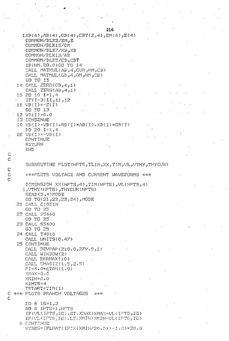
c
c
216 1XBC4) 1 ABC4l 1 GB(4) 1 CBTC2 1 4l 1 EMC6l 1 BC4l
COMMON/BLK2/BM 1 E CDl'"ii'Kl!··I./H.I< 1 !5./Gi'l COMMON/BLK7./RB 1 XB CD!\'I/1'IOH./E:LJ< ::. 3,,. ,:;n SO~lMO~I/BL~~/CB,CBT :[f(Nt1~EO~O)(;O 1'0 j.4 CALL MAT~ULCAB,4 1 CUR 1 NM 1 CBl Cr~;LL !···Jr~i'I'~'·!UL(GD l'4 _,Gl"i 1 !--1\Y! 1 CB) GO TO :t:>
14 CALL ZERDCGB 1 4 1ll CALL ZEROCAB 1 4 1 1l
:!.~:> l)(J :!.0 J:::j, }'4 IF ( I -<3) :1.1. t t:l. t :!. :;~
11 VB ( I ) '' -X:: C I ) GO TO l3
t2 v;:.n>,,o,o ::. ~~ CDH'J' ... J: HUE 10 VB<I>~:VBCI>+RB<I>*ABCI)i·XBCI>~~GBCI>
DO :20 I" :i. 1 4 /..~0 \)I;{ ( I ) ::: ··· t)B ( I )
CCJI>ITTI·II..JE F;:ETUf~H
El-1:0
SLJBROUTINE PLOTC~IF'TS 1 TLI~l,XX 1 TIM 1 VL,VT~1Y,T~·!YCUJ:~)
C *~f~GPL01'S VOL1'AGE AND CUF~RENT WAVEFORMS *~G~G
DI~IB~ISION XXCNF)1'S 1 4) 1 TIMCNF'TS> 1 VI.CNPTS 1 4) ::. I \!THY ( l·iF'Tb) I 'l'HYCUF( ( I,I!::·T~3)
F:EAD ( ::; _,. ~(·) 1'1!DDE GO.TOC21 1 22 1 23 1 24) 1 !10DE
:::.~:!. cr::!LI.. CJO:::J.l'-1 GC TO ~?.::>
;;:.~ ;.? C P1 L L ~:~ ~;~: 6 6 0 GD TO 2!:>
:i.'::l C Pr L!.. ~:;::'; fi., 0 0
i.~-4 c~~~LI.. 'I'·40l0 Cf'rLl.. l.JI'·H'iS ( 0, 47)
?!3 CDi··ITII>!l.JE CALL DEVPAPC210.0 1 279.0 1 1) Ct1I .. I.. WII\lDDl..o.J ( t.~ i C (r, LI.. l:-.':Fml'·'l!'r X ( :1. () ) c~;I.L c:~·!ASIZ<1.5 1 2o~i) P:[::4~o~~~TAN(1,0)
:~< i'-'l !:~) >< ::: () .. () XI'-'JII··.J:::() V 0 I·HHT~'>'"'~ To>Ti~l'n' "' T I !'I ( 1 )
r *** PLOTS BRANCH VOLTAGES *** c
L'D /:'. IG•":i.;::l DD n I F''no '" :1. t J,IF''Tb IF<VI~<J:F•1'S 1 IG) .. (;1'.X~IAX)XJ,IAX=VL(I~:·1'S 1 IG)
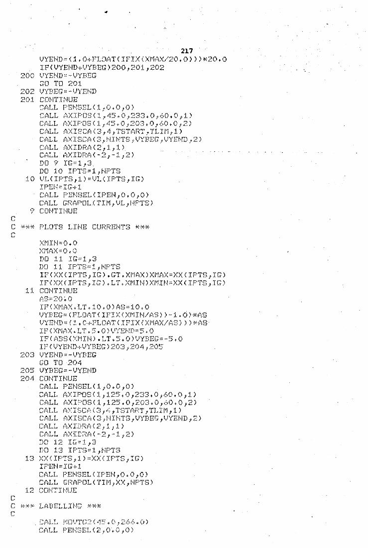
217 VYEND=C1,0+FLOATCIFIXCXMAX/20,0)))¥20.0 IFCVYEND+VYBEGl200 1 201,202
200 VYEND=-VYBEG ::; D 1' () ;:.' 0 1 1v'YBEG ::: ··· t)YE!,lD CD!,! 'I' I I'!UE ::AI .. L PBI,!SEL<1:0~0 1 0) C~AI~L AX:I:P(JS(l 1 45.0 1 233~0 1 6C)+0 1 1) CAI.I~ AXIF~OS<l. 1 45~0 1 203.0 1 60.0 1 2> CAI .. L AXIPCA(3 1 4 1 'rSTAF~T~1'l.Il1 1 1) C(:!LL i~lXJ~;:;C.~f:':) ( ~;3yJ\!IbiT~:~ J.\)YBEG tVYE:l··!D ,.2) CALL AXIDRAC2 1 1,1l CAl.L AXIDRA<-2 1 ·-1 1 2) DD '? IG<I.,::l DO 10 IPTS=l,NPTS
10 VLCIPTS,1)•VLCIPTS 1 IG)
CAl,L F~E~l8EL<If>EN 1 0.0 1 0) CM .. !.. Gf::p,PDL C TII'1 1. ~!J:.. ,I,IF"l'S)
? CDI·-!1' I i··!UE c C ~~*~~ PI .. C)TS I~INE CURRENTS ~0~~*
c
(., ...
c
DD :!.1 IG,=1 1 3 DO 11 IF'TS=1,~:F•'fS
IF<XXCif>1'S 1 IG>.GT.XMAX>X~tAX=XXCIP1'S 1 IG) IFCXXCIPTS,IG),LT.XMINlXMIN=XXCIPTS 1 IGJ
:1.1 CDt·ITHiUE
IFCXMAX.LT.lO.OlAS=10,0 VYBEG=<FL.OATCIPIX<X!1IN/AS))-1.0>*AS VYI:iND "' ( :!. , C.·I·Fl. OAT ( .T FIX ()(!''lAX/(.,>;)) ) ) ·l•';~B IF(XMAX.L'r.~5.0)VYE~!D:S~O IFCABS(,(MIJ,I).t.1'.5.0)VYBEG=-5.0 IPCVYEI~D·t·VYBEG>203 1 204 1 205
203 VYEND•-VYBEG GO '!'0 ::'04
220:5 VYBEG'-' ··VYEI'·ID 204 CDI'-ITI!,lUE
CALL PENSELC1 1 0,0 1 0l CALl~ AXIPOSC1 1 125.0 1 233.0 1 60.0 1 1) CALL AXI:~oSC1 1 125.0,203.0 1 60.0 1 2> CAt.L AXIS(:A<3 1 4 1 1'STAi~T,TLIM 1 1) CALL AXIE~E~A<3,~1IN1'S 1 VYBEG 1 VYEND 1 2> (~AL.L AXIDRAC2 1 l. 1 1) CALL AXit~AC-·2 1 ··1 1 2) DD :1.~~ IG::: :!. ,:;~ DO 13 IPTS•1 1 NPTS
13 XXCIF'TS 1 1)=:XX<IPTS 1 IG> IF'EI·I• IG+l (:ALI .. I~ENSELCIF'E!~ 1 0.0 1 0) CALL GRAPOLCTIM 1 XX,NPTS)
:i. :~ CD!"-!';:' I l··.n.JE:
[:AI .. ! .. M(JV1'[;?(4~~.0,266.())
CALl~ !='EI~SEI.(2 1 0~0,0)
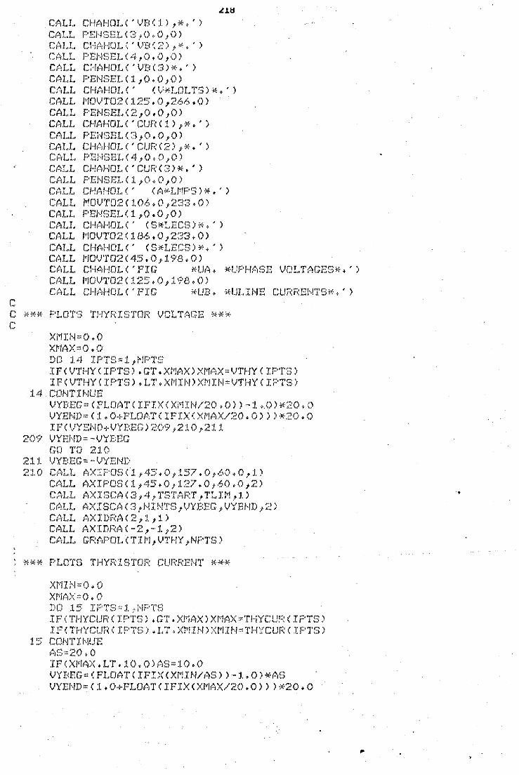
c
CALL CHAHOLC'VBC1l 1 *o'l CALL PENSELC3 1 0.0,0l CM.!.. CHr\HUL ( ' VB ( i.') 1 ;c., ' )
CALL PBNSELC4 1 0,0 1 0l CALL CHAHULC'VBC3l*o'l CALL PEI,Im::r .. ( :1. , 0 • 0, 0)
0.:.111
CiU .. l.. CHtoHDJ. C ' ( t)·i!·l .• D! .. TO:>) "', · ) CALL MOVT02C125.0,266o0l C.~l..L PENEELC:.~,o.O ,Ol CM.!. OH\ HO!.. ( 'CUF( ( l ) t l!·, ' )
CALL PEHSEJ..C3 1 0.0,0l CALL CHr~d IOL (' CI.JF; ( 2 l, ,,, .• ' ) CAI~L PBNSEl.C4,0,0,0) CALL CHAHOLC'CUR(3l•,'l CALL PENSEL<l,0.0 1 0l CALL CHAHOLC' CA•LMPSl•,'l CALL MOVT02<106,0 1 233.0l CALL PEHE~EL ( 1 ,O, 0; 0 l CALL CHr~HOX.. ( ' C3•! .. EC!:) H·, ' l CM .. L J•KJVT02 ( 1/3(;., 0 1 :?.3:-J. 0 l CA!..l .. CHI'oHDI.. C' ( SJt'Lf:CS l lf·, ' )
CALL /'ICJ'JTO:i! ( 4!:>, 0 t 1. 98, 0) CPrl.I.. CH0'rHOI .. (, r:·'IG )t~Uf~ I 1(·UF:'Hf.;~3r:-: 'v'(]!. .. T:~GE~:)~(·o,) CALL MO\.!T02C125.0 1 19S.Ol c,:'ir..I.. cHt1HOL c, FIG ·i(·UB, ·ir:UJ .. IJ-.JE cu;:i:r-~E!··.!T~:3~~(·,, >
XI'III-·1"0, 0 XNAX"-0,0 DO 14 IPTS=l,~IPTS IF ( VTHY C IP'I'f3) • GT, Xi''lAX) X/'li":X" ')THY ( IF'T3 1 IFC\.!THYCIPTSloLToXMINlXMIN=VTHYCI?TSl
:1.1.1 corrnr.n.m \.!YBEG=CPLOAT<IPIXCXMIN/20o0ll-1 •. 0)W20.0 VYEI'.IJl'" ( :1., o.;.FLOt:N IFIX C xr·!1~X1:2o, 0) ) l ·<?G. 0 IFCVYE~II)+VYBEG>209 1 210 1 2:l1
<.~0'7' VYI-::1-ID"-- VYBEG GD 'I'D 2:1.0
:i!.:l. :1. 'JXT<EG"' ... \.!YENJ> 210 CALL AX!F'OSC1 1 45.0 1 157.0 1 60.0 1 1>
CALL AXIF'OSC1 1 45.0 1 127.0,60.0 1 2l C.~,l,l.. f:,XI GCA (;;?., ·4 1 'I'!~~T;:':',F:'1' t TLI i"! .~ 1.)
CALI.. P.rX I Scr::l (~=~,I"! I !'-IT~:) i tJYBEG, VYEf,fD 1 :;~)
CALL AXJ:DRAC2 1 1 1 1) CALL AXIDRAC-2,-1 1 2) Cl'tl..l .• GF;f',PO! .• CTit'I,VTHY ,l,li::'T!3)
*** PLOTS THYRISTOR CURRENT *** X 1"/:fl'l '" 0 • () X!•·if;X "0, 0 DO .15 If~TS~:1t~lf:·1'S
IF C THYC!.!I'( ( I !"''I'f:)) , GT. X,...ii\X) Xf'IAX "THYCUF'; C I PTS) IFCTHYCURCIPTS).LT.XMINlXMIN•THYCURCIPTSl
1 !'; CC/,I'l'J HUE f.'of:><20 o 0 IF CXI''IM(, LT, :/.0, 0) i'o!:>,,:/.0, 0 VYDEG•CFLOAT<IPIXCXMIN/ASl)-l,Ol•AS VYEND,C1.0+FLOATCIFIX<XMAX/20.0lll•20.0
..
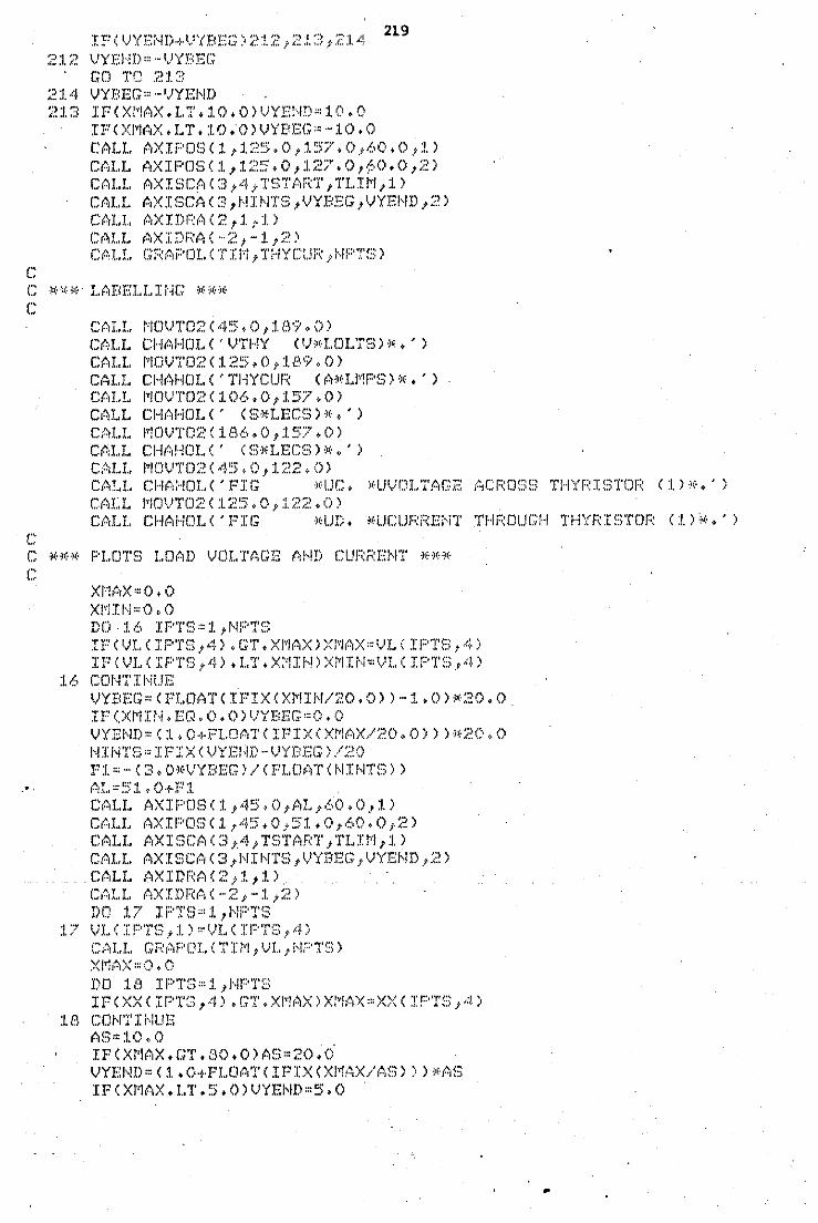
·c
IP(VYEND+VYBEG)212 1 213;214 ;:>. :1. ;~ \}Yf'.HD "' ·-VYF<EG
GO TC ~al~~
;~:1.4 VYBEG'" ··'.!YEI'ID 213 IPIXMAX.LT,:I.O.OlVYEND•:I.O.O
IPCXMAX.LT.:I.O;OlVYDEG•-10.0
219
CALL AXIPOSC1 1 125.0 1 157.0 1 60.0 1 1l CALL AXIPOSI1,125.0,127.0,00o0,2l CALL AXISCAC3 1 4 1 TSTART 1 TLIM,1l CALL AXISCAI3 1 NINTS 1 VYBEG 1 VYEND,2l CALL AXIDRAC2 1 1 1 1l CALL AXIDRAC-2 1 -1 1 2) C~Al.L GRAF·OI.(TII1 1 T~IYClJR 1 Nf~TS)
r *** LABELLING *** c
c
CALL HOVT02C45,0 1 189.0l C(.,LI.. CI··/(,HOL C ' VTHY I 'h' l .. DI..'f~:l l ;;, , ' ) CALL MOVT02C:I.25o0 1 189.0l CM.L CH(.,HOL C 'THY CUI'( ( A;•·L~·!PS) '!l, ' ) CALL MOVT02C106,0 1 157.0l CALL CHAHOLC' CS•LECSl•,'l CALL MOVT02(186~0 1 157.0) CALL C/··/(.,/··IOI.. I ' U:l·li LEC3 l ;, ,. ' l CALL ~!OVT02(4~~.0 1 122.0) CALL CHAHOLC'PIG •UC, •UVOLTAGE ACROSS THYRISTOR C:l.lv,· l CALL MOVT02C125~0 1 122.0) CALL CHAHDLC'PIG •UD, •UCURRENT THROUGH THYRISTOR Cl)~.·l
C *** PLOTS LOAD VOLTAGE AND CURRENT *** c
XI"·"/ f.; X"' 0, 0 X/•·:n-i•O,O D0-16 IPTS•1 1 NPTS IFCVI~<IPTS 1 4>.GT,XJ~AX)XJ1AX:=VLCIPTS 1 4) IFCVLCIF'1'S 1 4).I .. T.X~I~!)XMIN=:VL(IP1'S 1 4)
16 CD/"-ITII,iU:t-:: VYBEG•CFLOATIIPIXCXMIN/20.0))-l.Ol•20.0 IF(XMIN~EQ~O.O)VYBEG:=O.O
VYEND=Cl.O+FLOATCIPIXCXMAX/20,0lll•20,0 1~-1 I i·~t'X'~3 ;;; IF I>< ( t . .JYE!~!D ·-l)YDEG) /20 P1•-(3,0•VYBEGl/CPI..OATCNINTSll
.•. AL=51~0+F1
CALL AXIPOSC1 1 45.0 1 AL 1 60,0,ll CALL AXIPOSI1 1 45.0 1 51.0 1 60.0 1 2l CALL AXISCAC3 1 4 1 TSTART,TLIM 1 1l CALL AXISCAC3 1 NINTS 1 VYBEG 1 VYEND 1 2l CALL AXIDRAI2 1 1 1 1l CALL AXIDRAC-2 1 -1 1 2) DO 17 IPTS=1 1 NPTS
17 VL<IPTS 1 1)=VL<IF'TS 1 4) CALl. GRAF:·oL<TIM 1 VI .. ,~!F'1'S) Xl''itl)( ::; ()I()
DO 18 IPTS=1 1 NPTS IFCXXCIPT3 1 4),GT~X!~AX>XMAX=XXCIF·'rS 1 4)
:1.8 CDNTJ:l-.JUE AS=:/.(),() IPCXMAX,GT.SO,OlAS•20.0 VYEND=C1.0+PLOATIIPIXCXMAX/ASlll*AS IPCXMAX,LT.5,0lVYEND=5,0
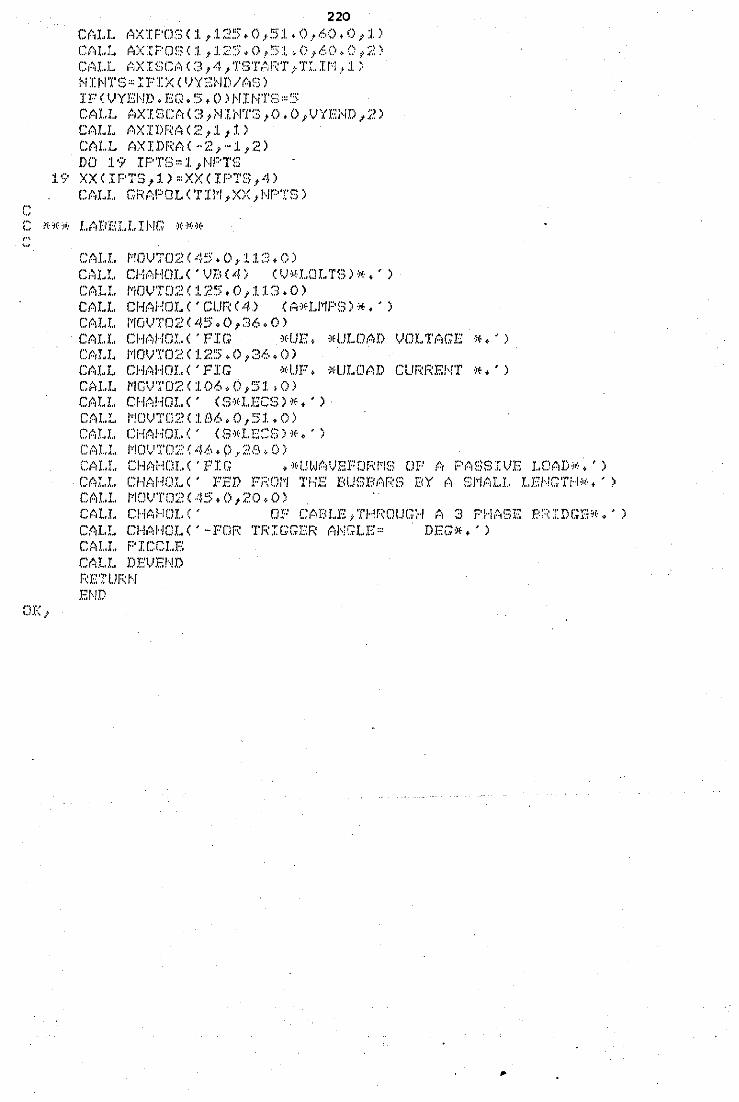
,., '·'
DI<t
220 CALL AXIPOSC1 1 125.0 1 51.0 1 60,0 1 1l CALL AX:rPOS<1 1 125.0,51}0 1 6().(),2' CALL AXISCAC3 1 4 1 TSTA1~T,T~I/~ 1 1; ~~I~I1'S=!FJ:X(IJYS~JD/AS)
IP<VYEND.EQ,5,0lNINTS=5 CALL AXISCAI3,NINTS 10,0 1 VYEND,2l CALL AXIDRA<2 1 1 1 1l CALL AXIDRA<-2,-1 1 2) DO 1? IPT~:;"' :/. 1 /·.fPT~o
19 XX<IPTS 1 1l=XXCIPTS 1 4l Cf.H .. I.. Gi~t\PC!L (TT!''/ 1 XX 1 HPTS)
CALL MOVT02<45.0 1 11S.Ol Ci~J! .. I .. CHi~J·!OI .. < 'tJD ( 4) ('.J~t·I .. CH .. TB) :I(·. ' )
CALL MOVT02<125.0 1 113~0) C1~LL CHAHOL ('CUI~ ( 4) ( (,·)r·LiviPS) '''. ' ) CALL MOVT02145.0 1 36.0l CM..! .. CHt,HCll.. ( 'I''IG ;r·UE, ·)fl.JLOAD VOLTr;GE ;,. , 'l cr.,u. i"'IOVTD:<'. < t:;>.::.>. o, :3,0 .• o l CALL CH.<\ HO!.. ('FIG '"'l.JF, ·lfl.Jl..OAD CUF\F::EI'-i'f .,, , ' ) CALL MGVT021106.0 1 51,0l Cf.:l .. L CHt.!--ICJL ( ' ( :3·H-l..ECS l ¥·, ' )
CALL MOVT02C186.0 1 51.0) CM. I.. CHAHDL ( ' ( S·)rLE::s l ;,. , ' i CAl.L MDVT02(46.Q 1 28.0) CM.!.. CHAHOL( 'f'IG , >r·l..!lvt;'JEFDf-\1'1::> OF (1 p,;::;~3IVE l..DAD·ii·,')
· CPti .. L CHAHOX.. ( ' FEr> FPDJl'l 'I' HE BUFBi~tF:[-) E{Y t·~ EJl'!PtLI.. LE!-..!GTH{I(·. ~ ) CALl.. MOVT02<45.0 1 20.0) cr.I .. L C!··1AHDr.. c ~ D! .... c~~·,BLE l THr~ouc:··f :.1 3 F'Hi:-:,sE r-:~PIDGE1(·.) · ) CALL CH(,HCL (' ··FDf< TRIGGEF~ r;f·,;GLE"' DEG;,,' ) C;'\!..1 .. PICC!..E CALL DEVE!·.fD m::TUF~/'1 mm
..
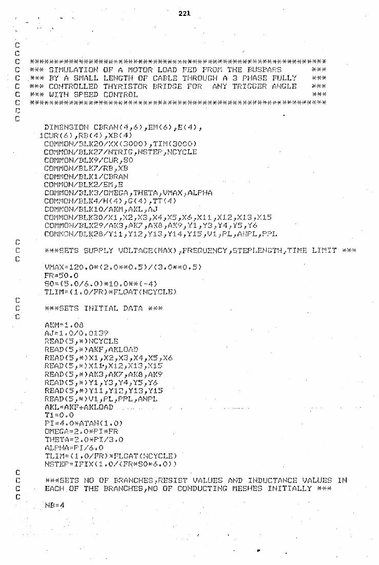
c c
221
C *l~f~~~*******~~***~f****if1f*~f*if**~f~fi~**1~*1~~f~~*i~1~i~if1f**lf*i~***ifif~fiE1f~f~f%
C *** SIMULATION OP A MOTOR LOAD FED PROM THE BUSBARS *** C *** BY A SMALL LENGTH OP CABLE THROUGH A 3 PHASE FULLY *** C ~Hi·~r· COHTI'\OLLED TI··IYF: :WTOI'\ BI'\J DGE FCm tol,l't TF: I GGER (d·.JGLE ·lHr··)(
C l1•·H· WITH <lf''EED CDHJ'f-Wl.. lHHf
c ******if~f**1fif*if****1fif%if#1f%1f¥****1f*~fif***if*****1f1f***1~¥1f*~f*1f1f~(** (., ., c
("'
DIMENSION CBRANC4 1 6l 1 EMC6l 1 EC4l 1 1CtJRC6> 1 RBC4) 1 XBC4)
COMMOH/BLK20/XXC3000l 1 TIMC3000l COi'Ji'"lCJI··i/BLlC'7 /~·IT!'\ I G, ,,!STEP I t··ICYCX..E COMMON/BLK9/CUR 1 SO COI'Ii'IOI,I/Bl.l<? /1'\B t XB COMMON/BLK1/CBRAN CDI'Ii'IDI"·.J/Jn . .l<2/El'i ,E CCJI"'WIDI·I/BL!Cl/Cll'IEG,<'J, THETA 1 Vl'i(;X t ALPHA COMMON/BLK4/HC4l 1 GC4l,TTC4) COM~!O~I/Bl.K10/AKM 1 AKL;AJ COMMON/BLK30/X1,X2,X3 1 X4 1 X5 1 X6 1 Xj_l. 1 X12 1Xl.3,Xl.5 COMMON/BLK29/AK3 1 AK7 1 AK8 1 AK9 1 Y1 1 Y3,Y4 1 Y5,Y6 COM!Ti(J~f/BL~28/Y11 1 Y12 1 Y13 1 Y14 1 Y15 1 V1 1 PL 1 AN!:'L 1 Pi~L
C ·lHHff;;ETG GUPF'l..Y 'JDl..Tr,CE 0'!.<'1X l 1 Ff(EOI..!El,ICY 1 GTEPI..E~IGTH /fH·!E LI!"'!::: T )(·:OH\·
c
(., ·'
V~!AX~120t0~~(2tO*a~Ot5)/(3.0**0•5>
FJC\<)0. 0 so~cs.o/6,0l•1o.o••c-4> TI..II'l ~ ( 1 ,. 0/PI'<l ,,,. FLCJ(;T ( HCYCI..E l
C ***SETS I~IITIAL DATA **~~ c
c
AKI'i"' :! .• on A~.r::: :1. ~ O/O. o:t~:3··? ~(EA!) (~)I lf) J·.JCYCI..E READC5 1 •lAKF 1 AKX..OAD READC5 1 •lX1 1 X2 1 X3 1 X4 1 X5 1 X6 READ<5 1 *)X1~;X12 1 X13 1 X15 READC5 1 •lAK3 1 AK7 1 AK8 1 AK9 READC5 1 WlY1 1 Y3,Y4 1 Y5 1 Y6 READC5 1 •lY11 1 Y12 1 Y13 1 Y15 READ(5 1 •lV1 1 PL 1 PPI..,ANPL Al<L = AI<F·J-i~,I<LOf.,!) T:l "() ' () PI"' 4, O·'''i~1'.<'li'!C 1 • 0 l CII'"IEG,"'<~, O·~+·:r '''-Fi'~ 1'Hr·:'T.'·.~ ::: :.~. O·l(·PI /~:~. 0 r~,LF'Hr~===FJ/6 ~ 0 TLIM=Cl.O/PRl»FLDATCNCYCLEl NSTEP=IPIXC1.0/(FR~f80*6•0))
r ***SETS NO OF BRANCHES,RESIST VALUES AND INDUCTANCE VALUES IN C EACH.OP THE BRANCHES 1 NO OF CONDUCTING MESHES INITIALLY*** c
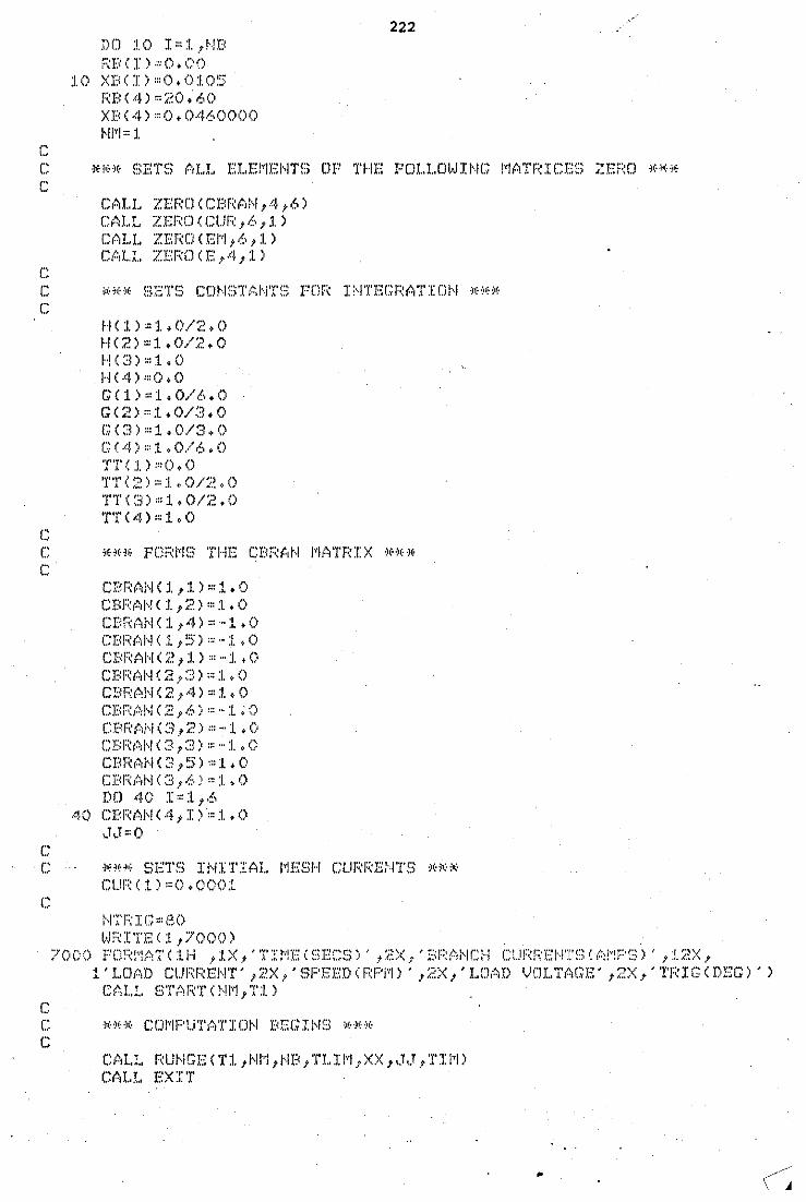
DD :!.0 I"':l. ,J,.Jn :-m ( r) "'o. "'l
:l.O XB (I):::(). 0:1.0~:>
F\BC4l"':i.~0.60 XBC4l"-0.0460000 ~.JI'J " 1
222
r *** SETS ALL ELEMENTS DP THE FOLLOWING MATRICES ZERO *** c
{"'
CALL ZEROCCBRAN 1 4 1 6) CALL ZERDCCUR 1 6,1) CALL ZEROCEM 1 6 1 1) Ct,I..L ZEF\D ( E, 4 t :l )
C *** SETS CONSTANTS POR INTEGRATION *** c
c
fH 1 l ~1 .on.o H <<?.) "-1, 0/2,0 HC3)":1..0 H < 4) "'0, 0 G(l)'-'1.0/6,0 G <:~) "1 , 0/:3, 0 G ( ~') "J. • 0/<l. 0 G(4) ::=l t0/6.0 '1''!'( 1.) ,,(),()
TT ( 2) ::::1. (> 0/~:~ "0 TT\ :3) ::: J .• 0/~.~. 0 'I"r< 4 ) " 1 • ()
r *** PORMS THE CBRAN MATRIX *** c
r
cnr:;p,,,, < J. , :1. l "'1 • o CBI:;~r~d ... J < :J. 1 ~?.) ::: :l • 0 er::::;,;,.,,< :1. , 4 l "···1 • o CBF~(.~!·,J ( :i. t :>) ::: ··:!. • 0 CX:<F\AI·,i ( i.' 1 :1.) "' ·•· J. , 0 CBF~P,!'-1 ( 2 .r~::) ::: :i. + 0 CBF: '"l'·i ( 2 t 4 ) " 1. • 0 CBr:~r:"~H ( ~~ 1 tf.,) ::: ·~ l .,- 0 c.r:~F:.·r.:.hi < ~3 l ~:~) === ·:·:t • o CDI'\Pd··i ( ::< t ::l) '" ··· :1. • 0 CBF\,;i'·i ( :l, ~)) '" :1. , () CBF~f:':,t-.i ( ~:~ .t (,) ::: :1 .• 0 DD 40 I"' :l f'o'
40 CBRANC4,I)"-J.,O ,1,1 "()
· C ·l>ilH•; SETf> Hii'l'IAl .. 11ESH GUF:F\E:·JTS '"'"''(·
c
c
CUr;~ ( :l) :::(). OOO:L
:·~ ·~· r-:: I G ::: l3 0 t-,1!'\ITE < :1. 1 7000)
700<) FO~:~~!A1'C:LI~ 1 1X 1 '1'I~!ECSECS)' 1 2X,'BF~A~!C~·! !:URRS~·!'f~~(Al4F'S)' 1 :l2X, l'LDAD CURRENT' 1 2X,'SPEEDCRPMl' 1 2X 1 'LOAD VOLTAGE' 1 2X 1 'TRIGCDEGl')
CALL STARTCNM 1 T:I.l
C *** COMPUTATION BEGINS *** c
CALL RUNGECT1. 1 NM 1 NB 1 TLIM,XX 1 JJ,TIMl CM .. L EXIT
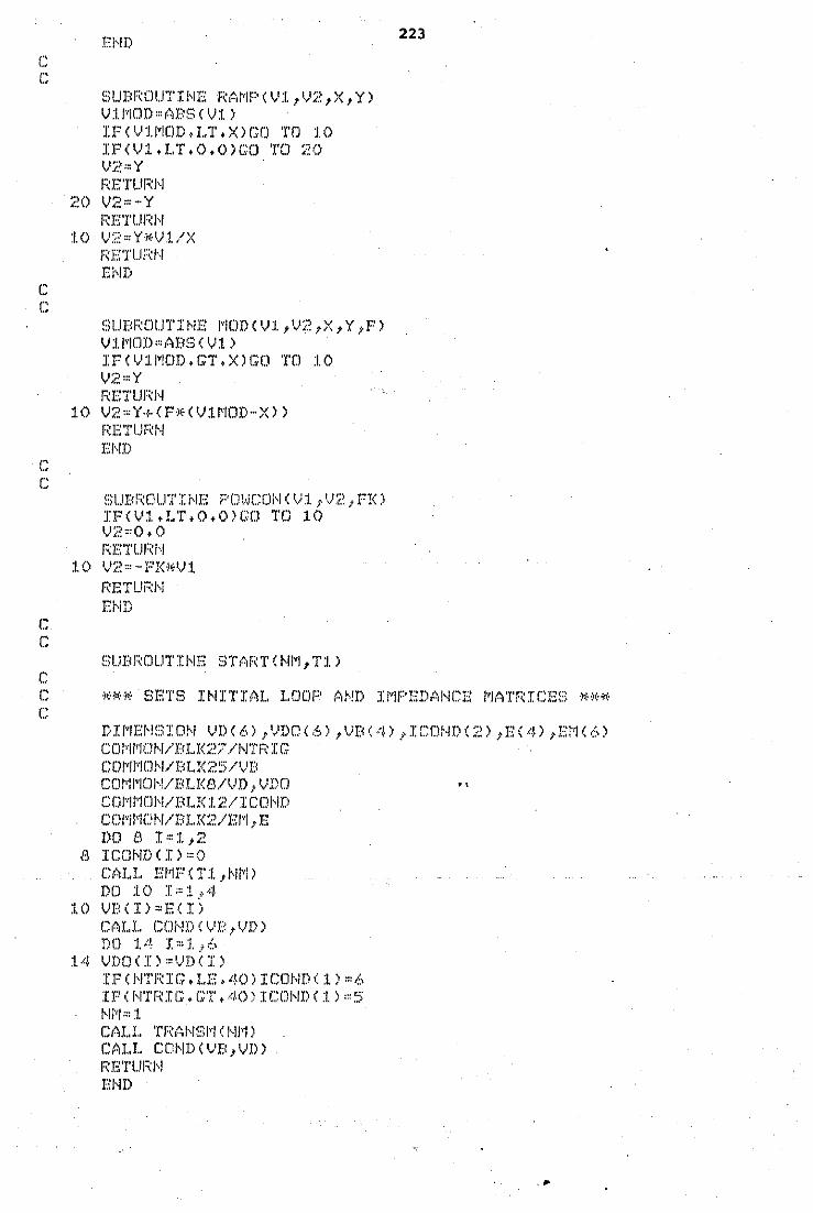
(''
c
c c
(., ·' (''
c c
c
SUBROUTINE RAMPCV1 1 V2 1 X,Yl V:I.WJD"-APSCV:I.) IF!VlMOD.LT.XlGO TO 10 IFCVl.LT.O,OlGO TO 20 v;;.~,y
I~ETL.I!'~H
<.~o v::!."' ·· Y i":ETURI··I
:1.0 V:i.',Y·i<V:J./X I'<ETUi'::N Ej;JD
SUBROUTINE MODCV1 1 V2 1 X,Y,Fl V 11''/0D '",~D~3 < V :l l IFCV:I.MOD,GT.XlGO TO :1.0 v;,~,,y
f\ETUI'\1~ 10 V2zY+<F•<V1MOD-Xll
RETI.JI'<J-.1 EI·.JD
SUBROUTINE POWCONCV1 1 V2 1 FKl IFCV:I.oLT.O.OlGD TO 10 v::>o. o 1\ETUI'<J·.J
:1.0 V:i.> .. ·Fl<l(·V:I. m::ru;:::J·.J Ef-.iD
SUBI\OUTIHE STARTCNM 1 T1l
223
r *** SETS INITIAL LOOP AND IMPEDANCE MATRICES ••• c
DIMENSION VDC6l 1 VDOC6l 1 VBC4l 1 ICONDC2l 1 EC4l 1 EM!6) COMMON/DLK27/NTRIG CO rll···!o ~I I l:~ ! .. :< ;~ ~~; /\,' B COMMON/J:-:LKB/VD 1 VDO COMMON/BLK12/ICOND COMMON/BLK2/EM,E no e r,1,2
B I COND ( Il "0 CAJ..I.. E/''IF ( T :1. 1 J-.11'1 l DD 10 I <l .A
:1.0 VE<<Il,ECil CALL CDHDCVP,VDl DO :1.;1 J>1,6
14 VNJ<Il"-VD<Il IFCNTRIG,LE.401ICONDC1lz6 IPCHTRIG.GT,40liCONDC:I.lz5 J-.1/"1 '" :1. CM .. I.. 'l'fMI,ISJ•·J C 1,11"1) CALL COHDCVB 1 VD) F<E'I'UF<I'I EHD
.~
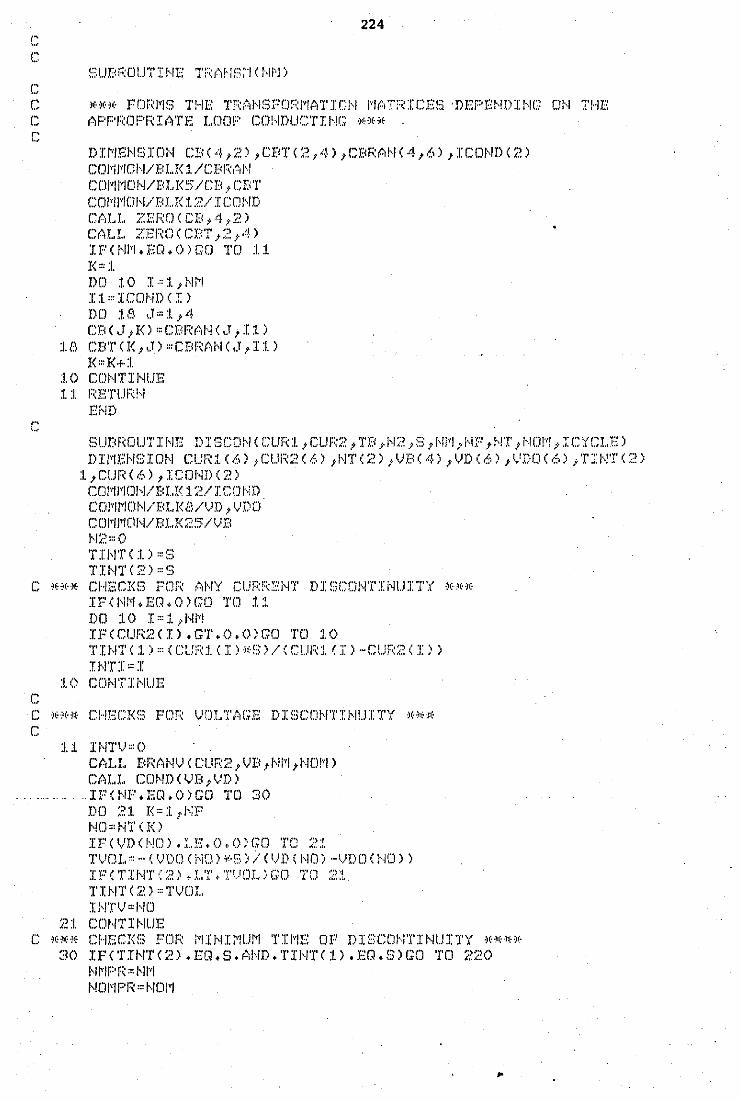
224 c c
SIJBROtJT!~IE 1'RANSr1C~IM)
c C *** FORMS THE T~ANSFORMATICN MATRICES ·DEPENDING ON !HE C APPROPRIATE LOOP CONDUCTING *** .
DIMENSION CBC4 1 2l 1 CBTC2,4l 1 CBRANC4 1 6l 1 ICONDC2l COMMON/BLK1/CBRAN COMMON/BLK5/CB 1 CDT COI··WION/BUC 12/ I COHD CALL ZEF~OCCB 1 4 1 2) CALL ZEI~OCCBT 1 2 1 4) IFCHM,EQ,OlGO TO 11 1<"' 1 DD J. 0 J> 1 1 NI'! I :l '"I COI·iD ( ::: ) DD J.l:l ,,1,,1,4 CBCJ 1 Kl•CBRANCJ,I1l
18 CBTCK 1 J)•CBRANCJ 1 I1l 1< •1<+<1.
10 CDI··i'l'IJ·<UH 1:1. l'mTUF<H
EHD
SUDROUTI~IE I>ISCONCCUR1 1 CUR2 1 TB 1 N2 1 S,~fl'I,~IF,~!T 1 ~!0M 1 I£:YCI .. E> DIMENSION CUR1C6) 1 CUR2C6l;NTC2l 1 VBC4l 1 VDC6l 1 VDOC6l 1 TINTC2l
1 1 CURC6l 1 ICONDC2l cm11'1DIVI<L!< 1.2/I cm-m CDMMDN/BLKS/VD,VDO CCWII''ICII·VBL1<:'5/VB I• I'-''" () TJI,I'l' ( 1 l <'> TII·-/TC::~l ·~>
C *~~* C~~ECKS FOR ANY CURRENT DISCONTINIJJ:TY *)~*
IFCHM.EQ,OlGO TO 11
c
c
DD 10 J> 1. J'l'! IF ( CUI'<2 C J) • GT. 0. 0 l GO TO 10 TIN1'C1)=CCtJR1CI)~f!3)/CClJl~1CI>-CUR2CI))
Il•l'l'J•I :1.() CDi•ITii,!l..IE
:1. :1. H/'l'V" 0 CALL BRANVCCUR2 1 VB 1 NM 1 HOMl CM .. I.. CD~!D (VB_, lJD l IPCNF.EQ,OlGO TO 30 DO ;?.1. I<" l t !·-T ~10 '" NT < IO IFClJDCHCJl,LE.O.OlGO TO 21 TVOI..•-!VDDCNOl*Sl/CVDINOl-VDOCNOll IFCTINT(2).LT,TtJ0L)G0 T(J 21 T I 1··11' ( :;.~ l '" TVOL I HTV '" HCl
:,~:1. CDt·ITII•ILJE C **~~ C~iECKS FOR ~!INIMUM TII1E OF DISCONTINUITY ~~**~
30 IFCTINTC2l.EQ,S.AHD.TINTC1).EQ,SlGO TO 220 I•Wif"f( • ~11"1 I~OI'IF'R" NDl1
..
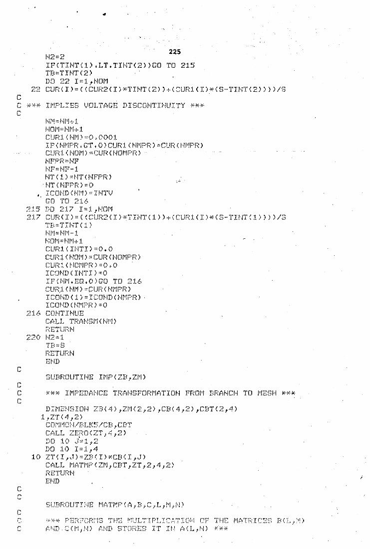
c
c
c
c
..
1--1~~ :::~-~
IPCTINTC1loLT.TINTC2llGO 'X' E< "' T :1:1-·1'1' < <!. > DO ::.~2 I'" 1 t t·ICJI"I
225
TO 215
22 CUR<Il•((CUR2<I>•TINT<2ll+CCUR1(Il•CS-TINTC2llll/S
!'ii"~! :::hil'11+1. H(JI'"I • l'll'i·f· :1. C'..JfU c HI"'! l "'(), ()001 IPCNMPR.GToOlCURlCHMPRl•CURCNMPRl CI..!F< :1. ( !··!Cll'"l l "' CLJF< ( !·iOI'If''l'() ~IFPF< •!'IF !··IF • ~IF- 1 !'IT ( l ) •!···IT ( HFPFO
·!··IT ( HFPR l '"() ICCH.JD <l·i:'"!) '" J!,ITV GO TO ;:~ :/.6
215 DO 217 I•1 1 NOM 2:1.7 cur-:: C I)::: ( ~ CUF\2 (I) ·l<:TJ:i\11' < :1.)) + ( CU!:~:1. (I) ~c·( f:)···TI!··.J'I' ( :!. ) ) ) ) /~3
'I'D:::'f:i:J--iT ( :L) l··iJ···I,,Ni·•J-·:1. I'!Cll':i'"l··ll'"i+:l. cuF<1 c :nrn: > '"o. o CUF: 1 C 1'!01'1) • CUI": ( HCWIP F<)
CUF< :. ( i·ICI"'IPf< > "' 0, 0 ICCJI··ID ( IHTI) •0 IFCNM.EQ,()lGD TO 216 CUF(i. ( !-.J!vf) =~CUF~ ( !\W!F'F~) ICONDC1)=ICO~ID<Nr:F·R> · ICOI·-!D ( !·.JI'"IF'F( l •0
; .. :! 16 COI·!T I i'ILJE
TB===B F<ETUF:I··I Etm
SUBROUTINE IMPCZB,ZM)
C *** IMPEDANCE TRANSFORMATION FROM BRANCH TO MESH *** c
c
c
DiME~iSION ZB<4l 1 ZMC2,2l,CB<4,2l,CBTC2,4) :l_tZ'f(·4 ,~;~)
COMJ101,1/BLK5/CB,CBT CALL ZEROCZT 1 4 1 2l r-., (''! ·j n {:: ., ·;~ M •• "'V \. .j, 1 "'""
DO :LO I":i. 1 4 10 ZTCI,JI=ZBCilWCBCI,J>
CM.!.. i'liYt'J•·IJ'' C Zi'"l 1 CJrr 1 ZT t 214 1 ;:.!) i'~ETUF~I'i Elm
SUBROUTINE MATMPCA,B,C,L 1 M,Nl
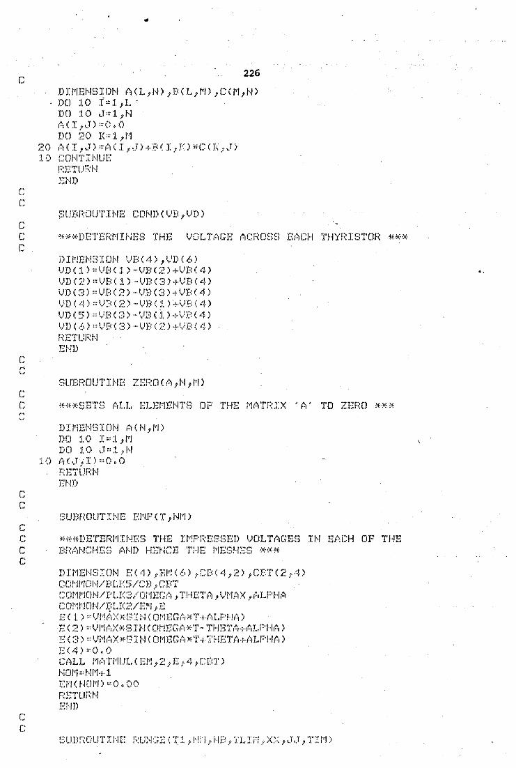
c
I"
c
..
226
DIMENSION ACL 1 Nl 1 BCL 1 Ml 1 CCM 1 Nl DD :!.() ;!',:1. 1 L · DD :1.0 ,,T,,:I.,J-.1 {~I (I }"~.T) :::() + 0 DD :;.~0 I<"' :1. ;1''1
20 ACI 1 Jl=ACI,Jl+BCI 1 YlwCCK,Jl :1.0 CDI,IT:i:J-.JUE
F:ETt..nH r.::HD
SUBROUTIHE CONDCVB,VDl
C ~••DETERMINES THE VOLTAGE ACROSS EACH THYRISTOR *** c
c
c
DIMENSION VBC4l 1 VDC6l VDC:I.l=VB<ll-VBC2l+VBC4l VDC2l=VBC:I.l-VBC3l+VBC4l VDC3l=VBC2l-VBC3l+VBC4l VD(4)=V3(2)··VBC1)~·VB(4)
VDC5>=VB<3>-VBCi>·~VBC4) VDC6l=VBC3l-VBC2l+VBC4l 1\ETUF:r·l El···!D
SUBROUTINE ZERDCA 1 N1 Ml
C ~~**SE1'S AL.L ELEMEN1'S OP THE MATF~IX ~A· TO ZERO *~f*
'" '"
(., ,, c
c
D HIE !,H:; I D 1,1 ,; (1'.1 1 /'1)
DD :LO I=:l.,l'l DD :1.0 ,.1=:1. 1 1'·1
:LO A<·.J(ll,,O,O r:;ETUF:i'i Ei'·iD
SUBRDUTIHE EMPCT 1 HMl
C ~(·1(··/(·DE'I'I·:f-(I.'IIHES THE :r:~·:pr::~ESSED VDLTAGEG IH EACH or-:o THH C BRANCHES AND HENCE THE MESHES *** c
c c
!)IMENSION EC4) 1 E~!(6) 1 CB(4 1 2> 1 CBTC2 1 4) COMMON/BLK5/CB 1 CBT CDMMDN/BLK3/0MEGA 1 THETA 1 VMAX,ALPHA COMJ~(JN/~LK2/EM 1 E EC1):::VJv!AX*SI~I((JMEGrr~f1'·t·AL.F~~-IA)
B(2)=Vl1AX~fSINCOMEGA)~T-T!~ETA·•·ALP~IA)
:E ( :;~ ) ~:: '·...'i.1!t1X ·)i· f:~ I 1\1 ( 01"~/l:-:Gr~r )(· T ·Y· TH:G'I'I~r+f.li .. F'Hf..i ) E(4) :::0~0 CALL MATMULIEM,2 1 E1 4 1 CBTl r·iDI'I '" I>Ji'1+ 1 r.::r'J ( riClr'l) '" o, oo I:;:ETUF<J··.f E;~.JD
..
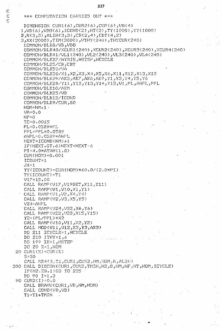
c , .. ',,,
227
DIMENSION CUR1(6) 1 CUR2C6l 1 CURC6l 1 VBC4l 1 1 VDC6l 1 VDOC6l 1 ICONDC2l 1 NTC2l 1 TYC1000l 1 YYC1000l 2 1 RC3 1 3l 1 ALINC3 1 3l 1 CBC2 1 4l 1 CBTC4 1 2) 3 1 XX (::lOO()) t T Il'l ( 3000) 1 \-'THY ( :i?.40 l 1 THYCUF< ( ::>40)
COMMON/BLK8/VD 1 VDO COMMON/BLK40/XCUR1C240l 1 XCUR2C240l 1 XCUR3C240l 1 XCUR4!240l COMMON/BLK41/VL1(240l 1 VL2(240l 1 VL3C240l 1 VL4C240l COMMON/BLK27/NTRIG 1 NSTEP 1 NCYCLB COl1!1(JN/BLr5/CB 1 CBT CD!'1[i~"IDI\i/BLI<~:::O/Vf~
CO~Il10N/BLK20/X1 1 X2 1 X3 1 X·4 1 X5 1 X6 1 X11 1 X12 1 X13 1 X15 COM!~(JJ~/BI~R29/AK3 1 AK7 1 AKB 1 AR9 1 Y1 1 Y3 1 Y4 1 Y5 1 Y6 COMMON/BLK2B/Y11 1 Y12 1 Y13 1 Y14 1 Y15 1 V1 1 PL 1 ANPL 1 PPL COi'li'"!OH/BLV 1 0/P:V!'I CDI"'II'I Cl ri/B L 1<1.' ::; /'JB COMMCJN/BLK12/ICOND COMMOri/BLK9/CUR 1 SO 1'-IOI.,J:::J .... II''I+:I. · vp,,o, o I··IF,,O TC> 0, 00:15 PL===O ~ o~::::eo.r·)~F·:c. PF''L"''''I'''l .. :<cO, 00:';1:)-:;-
NEXT=ICDHDCHMl+1 IFCHEXT,GT.6lHEXT=HEXT-6 PI''"·~, O·l~,'\Tt•i··l ( 1, 0 l Cl.!i::: < HDJ":) :::0 t 00 :t I CCll..IHl' '" l ,.TX,,:I. YYCICDUHTl=Cl..IRCNClMlM60,0/(2,0•Pil
l,.l:f.?::: J.:;;. (:() CALL F~AI~PCV17 1 V19SET 1 X11 1 Y11) CALL RAMPCV1 1 V!O,Xl,Y1l CALL F~AMP<V1 1 V2 1 X4 1 Y4) CALL RAMP(V2 1 V3;X5 1 Y5) \.'/.'.4 '" ,')~.;;::· 1.. cr., I.. I.. F~f.1!"li::• < 'v'-~.~-4, ')£.~~~ .t Xb, Y6) CAt.L RAI~PCVZ2,V23 1 X15 1 Y15) Y/.2::: ( f"L/f''f''L l '''X2 CALL RAMPCV10 1 V11 1 X2 1 Y2) CALL MODCV11,V12 1 X3 1 Y3 1 AK3) DO 211 ICYCLE=1 1 NCYCLE DD /.~:1.0 ITHY,,J.,f.> DO 19? IK=l 1 NSTEP DD i.~ 0 I< <l. _. H CJI"'I
20- CUl~1(K)~CtJF~(K)
G;==~::;o
(' "l l , ... " ., ' .. , .,... ("'l >"·.I ('l ,. .. ;,., '-'J··f ,. ·r··>·f •.. ~. "I" I·:' ,·I·· .. ,, ,1 , • ._ J.', ~-;- ~- ~;; • .:' .1 .1. j ..... ·1'\ •• .t .~ .. ' .·•, .C • .fl'• '• j • 'i .. .1 I' • t I'\ i {··, 1., · · ·~ ··
~300 Ci~LL DI~SCDI\l ( CUF\::1. ,CU!:\2 l '1'/.,.i:f.t·-i 1 H2 ,~;;, J··.Jr··J 1 J'.IF .tl··!T ,J-..1Dl~"l j· I CYCLE)
DO <:;"() :1> :1. 1 3 ?0 CLm;;:; <I)"'(), 0
CALL BRANVCCUR1 1 VB 1 NM 1 r10Ml c,~.u .. cmm < vn, \.'D' T:l =T1+'I'I'"IJt·l
..
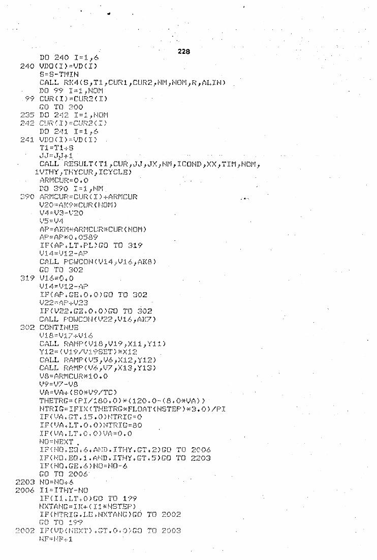
DD "'40 :J> :1. 1 6 240 VDOCI)=VDCI)
S::=S···Tl~"IIH
..
228
CALL RK4CS 1 T1,CUR1 1 CUR2 1 NM,NDM 1 R1 ALINl DD ?9 I::: :L .t ~·lDJvl
99 CURCI)•CUR2(I)
:=.~:=~=> 2-4~::
D Cl :i'. 4 ::.' :J> 1. 1 i·K!I"'I C-!.H~· c :r > ::: cur~2 ( :::: DD :=.~ .•:!- :1. I ::: :1. t tS VDD ( I l " '..'D < I ) T:l. ==='X' :I.+~> ~x ~.r === ~.r ~.r + :!. CALL RESULTCT1 1 CUR 1 JJ 1 JX 1 NM 1 ICOND 1 XX 1 TIM,NDM,
1VTI~Y,T~~YCUR 1 ICYCI.E) N~I-'!CLJF~ '" (). 0 L'rD 390 I::: :1. 1 1·,WI
:J90 ARMCUF~=C!.JRCI>+ARMCUR
\.-' :> ::: t) .-:".~ AP=AKM~ARMCCR~CURCNDMl
IFCAF·~LT.F~L)GO TO 319 I.) :t -4 ::: \) :1. ? ·~ l{':i F' CALL PGWCONCV14 1 V16 1 AK8) GC; TO :iO?
3:!. 9 I,_}J.,'f.·,:::O • ()
IF (V~:~:~~. G!-~ ~ 0 ~ 0) GO TD ::io;,~
CALL POWCDNCV22 1 V16 1 AK7) ~:~OL.~ CDJ··-IT J: i\IUE·:
t,) :L E\ ::: t) :L 7· .. : .. \} :1. ,:;.,
CALL RAMPCV18 1 V19 1 X11 1 Y11l Y12=(Vl.9/V:i.9SE1')*X12 CAL.L F~A~IPCV5 1 V6 1 X12 1 Y12) CAI.L RAMPCV~ 1 V7 1X13 1 Y13) V I:)'" ,~, ;::~ 1'1 C LJ ;::; lt :1. 0 , 0 \.-'9::: 1v 1? -\}8 VA=VA+<SO~V9/TCl
THETRG=CPI/180,())¥(120.()-(S,O•VAll NTRIG=IPIXCTHETRG~FLOATCNSTEPl~3.0l/PI IFCVA~G1'~15.0)NTRI(;::O
IFCVA.LT.O.OlNTRIG=SO IFCVA,LT.O.OlVA=O,() 1'·1 D "' I··IE / 'l' . IF~G!Cl.EQ.6.A~·lD.IT~iY.GT~2>GO 1'!J 2006 IF (!·-~Cl, EO, :1 .• (.:,I .:I), I THY, GT, ~))GO TO :i.!20::J IPCNO.GE.61NO=ND-6 GO TO ?006
:i.' I.' 0 3 r·l 0 '" N Cl+ 6 ;:,~006 I 1 '"I THY ···/'·ID
IP!Il,LT,OlGD I'D 199 NXTANG=IK+<Il•NSTEPI IFC~ITRIG.LE.NXTANGlGO TO ?002
1-iF'"I·>F·:··:I.
.....
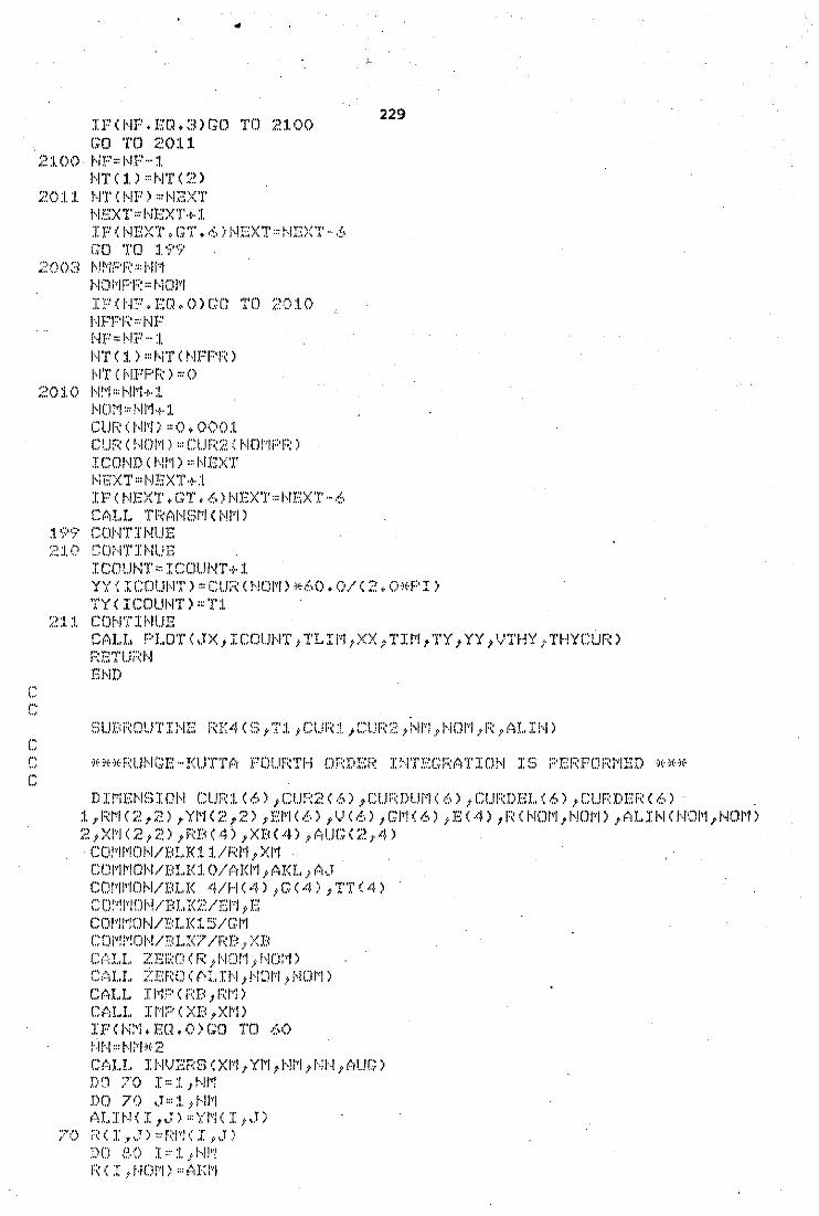
" ~--·
c
c
IFCNF.BQ,3lGD TO 2100 GO TO 20:L1
2:1.00 J··iF'" 1•1<'' .. ·1. l··l'l' < 1 > '"1·-rr c 2 >
2011 NT<NPl=NEXT HEXT,HE:XT+l J:F<NEXT~(;T~6)J~EX1'=~1EX'I'··6
GO TO 1?? 200~:~ J\!!\'/F'J?.·::J\11'·1
t·IDI'IF'F:'" l'·lCWI IFCNF.EQ,OlGO TO 2010 J·.JFF''F< '" HF' I··IF=HF .. ·:I. I··! 'I' ( :1. ) '" l'·l'l' < J··IFF'F~) I·· IT C I•IFF''f< l = 0
:i.~O :i. 0 1··!!''1 '" J·.IJ"I + 1 1•101'1 '" !•11'1+ 1 CUI~< 1··11'1) '"0. OOO:l CURCNOMl•CUF:2CNOMPRl I CDI·.JD ( bii"l) '"J·.JE\T I•IEiX'l' '" I·!EXT + .'1.
IFCNEXT,GT.6lHEXT=NEXT-6 Co!OLL 'X'I'<t1i··!EWI ( 1•!1"1 l
:l '?? CONTII•IUE ;:~:1. 0 C:DJ·JT I I•IUE
I CO!...It.f'l' =I COUNT+ :l
229
YY ·~ ICOUI\IT) ::: cu;:~ ( !··-!()1'11) ~(·,1,(). 0/ ( 2 y ()~(·PI)
TY < I CDI..JI•I'n = T:l
CALL PLO'l'CJX 1 ICOUN'l' 1 TLIM 1 XX,TIM 1 TY 1 YY,VTHY,THYCURl F':ETUF<J·.J EHD
SUBROUTINE RK4CS 1 T:J. 1 CUR! 1 CUR2,NM,NOM,R,ALINl
C~ *~~*F~LJ~J(;E--KllTTA POLJF~T~I OF~DEF~ INTEGF~A1'IC)N IS F'ERFORMED ~~** c
DIMENSION CUR:J.(6l 1 CUR2C6l 1 CURDUMC6l 1 CURDELC6l 1 CURDBR!6) 1 1 RM<2 1 2l 1 YMC2 1 2l 1 EMC6l 1 VC6l 1 GMC6) 1 EC4l 1 RCNOM 1 NOMl 1 ALIN!HOM 1 NCJMl 2 1 XMC2 1 2l 1 RBC4) 1 XB<4l 1 AUGC2 1 4l
COMMON/BLK11/RM 1 XM COMMON/BLK:I.O/AKM 1 AKL 1 AJ COMMON/BLK 4/HC4l 1 G!4) 1 'l'TC4l CD!''!I\'!DH/BLI<t.~/EI···I J.E: COJ·'l!"!OI.J/);::l .. K 1 ~)/GI'I COMMON/BLK7/RB,XB CALL ZE20CR 1 NOM 1 NOMl '''All .. ,., .. f'•'''''·" ]'J·J J·'"l"l 'l''l~J) \,,J··j ,, ,, ,(.,.\',", •,l,.l 1, !·-~ ,,,,., ·. j '! ,,,1 ' }' J\ l., 1·
CALL I I'IF" ( i'':l) 1 FW! l ct,J..L :rJ··n::·cxD,x~-,,
IF C l·i:•·J,l:(]. 0 l GO TO 60 r·-/H:::I ... Ji"~l:•(·/.~ CALL INVERSCXM 1 YM 1 NM 1 NN 1 AUG) DO 70 J> :!. 1 ~-W!
!) Cl 7 I) ,,l '" :!. 1 J··.IJ'J ALIN<I 1 J>=YMC:[ 1 \J)
70 ~~(I 1 J>=RI~(I 1 J) I! D ~-:\ 0 1 ::· :!. J !·,WJ F~ ( I .t 1'·1 0 r:! ) ::: ~~~I< :·~1
C' c
c
80 RINOM 1 Il=-AKM 60 RINOM,NOMl•AKL
ALINCNOM,NOMl•AJ DD :!. 0 I<"' :1. 1 I··ICWI CURDUMCKl•CUR11Kl
:LO CUFWEU!O '"0.0 DD ::~0 IF:L!!··I'" :1. ,4 T2=:1'1i·T1'<IRU~I)~~s
CM. I.. r::"1F C T::~ 1 1··!1'1 l
230 .
CALL CURD01'(CURDUM 1 CURDER 1 NDM 1 ALIN 1 Rl DD ~:::o I<::: :L J· J'-.1Dti CURDELCKl=CURDELCKl+G<IRUNl*CURDERCKlMS
30 CURDUMCKl=CUR1CKl+HCIRUNl*CURDERCKlMS ;~o CDH'I'It.,IUZ.:.:
DD 40 I<= :1. 1 I,ICl/'1 40 CUR2CKl=CURl!Kl+CURDELCKl
Ct·~~r..r.. !''/r~'I'!''lUI .. (V ,J-.JDI'i ,Cl...l1:~2 1 f..ID!\'l }·r~) DD :>O I:: l .i' 1.,1CWI .- · • ,.
50 VCil=EMCil-VCil CALL MATMULCGM 1 NOM 1 V1 NOM,ALINl F~ETUF:~J·~:
Ei··iD
SUBROUTINE CURDOTCCUR 1 CURDER 1 NM 1 YM,RESl
C ***DBTAI~!S T~1E DERIVATIVE OP 1'~~E MES~i CURI~El~1'S *** c
c
c
DIMENSION CURC6l 1 CURDERC6l 1 EMI6l 1 RESCNM 1 NMl 1 1YMINM 1 NMl 1 VDROP<6l 1 EC4)
CDt .. !tDI'.I/BI..J.<~:.~/I-:-:1"'·1 i I-:·: . CALL MATMULCVDROP 1 NM 1 CUR 1 NM 1 RESl DD 10 I"' :1. 1 1·-11'1 VDROPCil=EMCil-VDROPCil
:l.G CDI·iTii:·!I.JE CALL MATMI.JLCCURDER,NM,VDROP 1 NM,YM) !'(ETUF:I··I r:::·m
SUBROUTINE MATMUL;Y,NY 1 X1 NX 1 Al
C ***GIVES THE PRODUCT OF A MATRIX ACNY 1 NX) AND A C ***VECTOR XCNXl AND STORES IT IN VECTOR YCNYl *** c
c c (' '·•
DIMENSION YCNYl 1 XCNXl 1 ACNY 1 NX) DD :!. 0 I::: :l 1 f··./'1 Y(:J:):::().()
DD :1.0 \.r :\: :i. t h-I X :l.() YCI>=YC:~)+ACI,\J)*X(,J)
F(E';'!..JI'(I··! Ei··./D
SUBROUTINE INVERS<X,XIN 1 N,~iN 1 AUGl
C *** FINDS THE I~IVERSE or A MATRIX X or ORDER N ,, ~---
("
DI :-~;r:HE>:~:C~i"--1 ~< (!"I i l··-1) _t ::<I!·-! ( i··.! -~ 1·-.f 1 ;· t,I.JG < 1·-1 J· i··!f··-1) DD :1.0 I::: :i. 7 ~---!
("
c
!''
'·'
231
:rFCABS<.XC:r,J)),G1'.:l,OB-·08)G0 TO 10 X\I 1 ,.T)=O.O
:!. () CCll,l'l' I i'IUE !10 :1.:1. J>:l. 1 l··r PO :l.t ck .1 t H
11 AUGCI,Jl=XCI 1 Jl DO 12 I•=J. 1 H i'IY =~·I+ :l !)fJ J. :~ cl"' J··IY 1 1'11'·1 IFCI-J+Nl18 1 14 1 :1.3
:I.::J r·,UGCI,,.Tl=•O,O GC TCJ 1:'.
1·4 (,t.JGCI,cll=:! .• O :1.1.~ CD~\l'J.'IJ·,!f...!E
DOE: 1<=1 1 ~1 DD :1. r.:·. I ::: :L 1 I··.J IF ( I MO!{) ;,~·4 J i?.~3 j £.~4
24 IFCAUGCI 1 Kl,EQ,O,OlGO 1D :1.6 23 IPCAUGCI 1 Kl,EQ,O,OlGO TO 17
Dl..ll''i!''IY=AUGC I 110 DO 1 B cl"' :1. 1 i•ll···l 1'1 =• Hl···l+ :l ·-,J A!.JG<I,M>~AUG<I 1 M)/DlJM~!Y
:/J} C~JJ--.JT:a·.JUE
:!.1':. CDr·iTII,IUE DD :1. ~:5 I.. ::: :l f I·,J IF' (I..~· I<)£.~::> 1 :1. :;; ,2~>
25 IFCAUGCL,Kl.EQ,O.OlGD TO 15 DO l. 9 1'1=• :1. 1 HI··I
19 AUGCL,Ml=AUGCL,Ml-AUGCK,M) :1. ~; COl•!':(' I t·iUE
])() :C?.() I= .t tH DD :i.'O ,J '" J. ; 1•11··1
I~CAUG<I 1 M>.EQ.O.O)!~O TO 20 AlJGCI 1 !1>~AUG<I 1 M)/AUGCI 1 I)
?0 CD!·-.JTI!--H.H:·: DD ~:~:1. I::: :J. ;-hJ r·IY=•I··I+:I.
·DC ~;.~ l ~.T ::: J-.Jy t l'-ii··.J I<=::.,J MO!\!
21 XIJ~<I 1 K>=~AUGCI 1 J) :1.7 RF::Tt.mt-1
E!-.!D
C F'RINTS F~ESLJLTS )f*)~
c DIMENSION C:URC6l,VBC4l,XC4l,ABC4l
1 1 :[CONDC2) 1 XX<10()0) 1 TIMC1000) 1 VTHY<240) 1 T~~YClJR<240) 2_;-l.)J)(/.) lt.)l)[l(,f.·,)
COMMDN/BLKB/VD 1 VDO CD I'' I ~IC J·.f / D L r: ;:.~~·;/VD CDMMDN/E<LK40/XCUR1C240) 1 XCUR21240l;XCUR3C240l 1 XCUR4C240l COI'Ii'lDI-i/})l,I<41/\.'L :1. C :'.'40) , VL:?. C240 l _.l,1Lcl C:i'-10) _.1,'!..4 ( ;::40) CCWII'!Cli,I/BLI<~) () /VA
..
c (., "
c
c
232 COJ•WJOI--I/BLI<5' /HTF~ I G 1 t·lSTEF' 1 1--ICYCLE CCWII'HJ I'll B! .. I< :1. cl/ •"~ B AB I<'" CUF~ ( HOn)
DD :1.0 I" 1 ,a :1.0 X\:I:):::~)BCI>
X<Al "···Vr!C4) IF<ICYCX .. EoEO.~ICYCLE)GO 1'Cl 12 GO TO u:.
J. ;~~ XX ( ,JX) :::;;DB TJI'"i ( ~.rx) ===T:i. XCI...!!'( :I. (,JXl '"M·:!( :1.) XCU/::.:2 ( ~.TX) :::t:D ( ;2) XCI.Jf(3 ( ,JX l "."~El< :3) XCl.JF~4 < ,J)( l "r~B ( 4) 'P .. :l. < ,JX) '"X< 1 l
V! .. ::l(,JXl '"XC:)) I.JL .. ·I ( \.T)() :::X ( < ) THYCUi'( ( ,J)() '" 0, 0 IFC!~M~EQtO)GO TO 15 DD :i.l I" :1. ;- i··li''l IFCICO~!DCI).EQtO)GO TO 11 IFCICONDCil.GT.2lGO TO 14 \JTHY < ,JX) :::0 l· 060 THYCURCJ/l•THYCURCJXl+Cl.JR(:J:) GO TO 11
14 IFCTHYCURCJXl.GT,O.OlGO TO :1.1 THYCUF': ( ,JX l '"(), 0 V THY.< JX) '"VD ( ::. l
GO TCJ 6:1. :1. ~:; !...JTHY ( \.TX) ::: ~)D ( :l ) 6:1. ~.'fX===~.TX··:-·:1. 16 1'1:~IG==FI .. (~ATC!~TFi:IG)*60.0/40.0
WRITE<1 1 1000)T1 1 CAB<I> 1 I=1,4) 1 ABB 1 X(4) 1 TRIG :1. j J ,J! ~·1 1·0
1000 FOR~!ATC1H 1 1X 1 F9.7 1 3C2X 1 FB.2> 1 5X 1 f8,2 1 5X 1 FB.3 1 5X 1 FB~3 1 15X 1 F7,3 1 2X 1 I6 1 2X 1 F9.4/)
.·SOO I'':ETI..II'':H EHD
SlJB~OlJ1'1NE B~ANVCCUR 1 VB,~!M 1 NOI1)
Dl:fiE~iSIC)l'l CIJR(6) 1 VB<4> 1 GP!<6>,C3C4 1 2) 1 RBC4) 1 1XB14) 1 ABI4l 1 GBI4),CBTC2 1 4) 1 EMC6l 1 EI4)
CDI'(/I''!CJI··-i/Bl..r<~:~/EI''I }· E: COMMOH/BLK10/AI<M COJ·•!i'IDi,I/DI..l<l ~5/GJ···J COJ11~DN/BLK7/F~B 1 XD C CWI!'!OI··I/t:.l..I< 1. ::l/ t,B COMMON/Dl..K5/CB,CBT IFC~JM~E(l.C)>GO 1'0 14 c~~:LL 11'1PIT'I''IUL ( P1E: t ,;f l Ct.JF:~ t /'·-!1~-; J c~:-:)
Cr~iLI.. :·•Jt:TI' .. !UL ( G~:ll"·-~ _;· r~l"! 1 1'-!1'11 J-C.r-: ~~
GC 'J.'D :L!:::
. '
c c
..
14 CALL ZEROIGB 1 4 1 1l , C,1,Ll,, ZEI'((J (AD 1 4 1 :1. )
:/5 DO 1.0 J> J. , 4 IF C I ·-:3) :1.1 1 j.l t :t:'.!
1:1. ~'B<Il"'"'E\Il GO TO :1.3
l :? VB (I)::: tlKI ... I:,,:.Ct.JI;;: ( I'!Dl ... l) l ::l COl-i'!' J i'IUE
233 .
:lO VB<I>=VBCI)+f~B<I)*ABCJ:>+X3CI)~fGB<I>. DD ~~~0 I::: :t t 4
"·'0 Vr:< ( I ) '"··VB ( I ) F\ E '!' U :::: 1··1 Ei'ID
SUBROUTINE PLO'l'CNP'l'S 1 ICOUN'l' 1 TLIM,XX 1 TIM,'l'Y 1 YY,V'l'HY 1 'l'HYCUR) DI!~ENSIO!~ XXCNP'rS) 1 'rii~CNP1'~3>,YYC1000>,TYC1000)
1 1 VTHY<NPTS> 1 1'~1YCLJF~(NF'1'~~) CO!~i~O~!/BLK40/XCUR1C240) 1 X(:LJ!~2C240> 1 XCUR3(240> 1 XCUR~C240) COMMON/BLK41/VL.1(240l 1 VL2(240l 1 VL3C240l 1 VL4C240) !;;E/)D ( ~:> 1 ·)~) J··iODE CO TOC21 1 22,23 1 24> 1 MClDB
;:!1 c,~:,LL Cl0~5:1.1'1
GO TO i.?~}
~:.~~3 C Pt L L ~;:: ~:> .~, 0 0 GD TO :~~)
24 CP.:LL '!'40:!.0 Ci~1LI.,· U1\IIT~:3 ( 0" 47)
:~~:> CD~,!T I i\lUE CALL DEVPAPC210.0 1 279.0 1 l) Ct,LL [,,III·mOGJ ( 2)
CALI~ C~IA~~IZCj .• 5 1 2<~~) XI'•! A X"' 0, 0
HI!··.JT~:~:::4
TBEG,TII'I < :1.) C o)(·~··i··)(· F='LO'X'S :t-:F~P~t··ICH 'v10L'tf.:iGES ~(··:n:··)(·
c
IPCVId1Cl:F'TS>~(;T.XMAX>XMAX=VI~1CIPTS> IF ( tJ1 .. 1.~ < I F''TG) <> G:T ~ ><l\'IAX) ><J·r;tJX :::\.J.L::? (I PT~:;) :1: r· ( t)I..3 ( IF'TS) ~ GT + Xl'"lr~X) Xl'"iAX :::V! .. ::l < I F''I'f:~) IFCVL1<IPTSloL'!'.XMIN)XMIN=VL1(IPTSl !FCVI~2<1F''fS)tL~·.xr~IN>XMIN~VL2CIPTS> :;:F< 1·...'I..~:~ { IF''I'f;) ~I.. 'X'. XJ···Jif·.J > Xr .. iJJ-.!:::!.)1..:.~ ( IPT~3)
1:\ CO>-!'l'II···Il.!E VYBEG=CFLOA'l'CIFIXCXMIN/20.0l)-1,())M20.0 VYEND=C1.0+FLOATCIFIXCXMAX/20,())))M2(),() IPCVYEND4·VYBBGl200 1 201,202.
':)(\'~ ~ .. ~l .< ••
·~~ 'l ., .... \,, ...
'JYEI•ID"' ... \,iYE<EG G!J 'I'D ?01 ',Jym;:G= ... \ 1\'Er.JD CDI·ITII··IUE Cr::1LL F'!::·:! .r;:;:~::-;r., ( ;[. l 0 ~ (" t 0) C~Al~L. AXI;·:·o~3(j.~4~~~()t2~~~~.(),6()~() 1 :!.)
-'~AI~L. AXI!:•(J~3(1 1 4~~.0 1 203.0;60.0 1 ~)
Ctli..L ct.r . .r .. CtlLL Ct~I .. L :J:G::: :J.
CM .. !.. f"EJ··IGE!.. <I ;::·r;:~l 1 0. 0-' 0) GO T0<7 1 9 1 10l 1 IG
7 CALL GI'\AF'OL ( 'l' I 1'/ t VI.. :l. , ~-11''''1'::;) IG,IG+:l GCJ TO 6
9 CALL GRAPCJJ..CTIM 1 Vl..2 1 NPTSl IG"•IG+:I. GO TO 6
10 CALl. GRAPOL<TlM 1 VL3,NP1'~~). ('' ·:OHHt· F'LOT::> I..IHE CUPI'(E/-!'n:l 1HHt
c XI''/ I'''"' 0, () XI''IAX"•O. 0 DO 11 IPTS•1 1 NF'TS IF ( XCUF\1. C IF'Tf:3) , GT. XI"!(.,)() XI•·/,'\X ~XCl.N :l ( I F''!'i:)) IF< XC:UF<::.~ ( IF'TS) • GT, Xi•/t,X) X/'/,'\X'-'XClJf::t'. ( JTT~')) IF ( XCUF\:3 ( IPT~:>) , GT, XI''! M() Xl•'lf.,X"•XC::I..JF<J ( JPT~'l) IF ( XCI.Jf::l ( IF"l'U) , LT, XI"IJ:r.J) X/"/Ici•"XCUF\1. C If''TS) 1F<XCUR2(:[F''fS).LT.XI~I~1)X/~IN=XCU!~2CIPTS)
IP(XC~IJR3<IPTS)tLT~XMI~f)XMI~1=XCUR3CIPTS)
:1.1. CC!!·!TH!UE VYBEG,(FLOAT<IFIXCXMIN/:/.O,Oll-l.Ol*:I.O.O tJYE/.1!) "' ( 1 , O+FI..Dt~'!' ( IFI X ( XI'!AX/:1. 0, 0) ) > '" :1.0 ,. 0 IFCXMAX.LT.2.0lVYEND'-'2,0' IP<XMAX.LTt2.0>VYBEG=-2.0 IFCVYE~ID·~·VYBEG>203 1 204 1 205
;~O::l VYE/'.!Dm ·-',JYBEG GO TO 2!04
20~5 VYBEG "' -· VYE~iD 204 CD~ITHIUE
IFCXMAX-:I.,()l12 1 13 1 :1.J :1. :i!. VYEI'Hl" J.. 0
VYF!EC> -1. , 0 :1. ::l CO/',I'!.'H·II.JE
CALL P.E/·./EEL ( 1. 10,0, 0 l CALL AXIPOSC1 1 1.25.0 1 233,0 1 60.0 1 1l CALL AXII~OSC1 1 125~~0 1 208~0 1 60.0,2) CALL AXISCA(3 1 4 1 TBEG,1'LIM 1 1> Ct.I.L t.'.X:fSC,'\ ( :J 1 ~-IH-i'I'S ,VYBEG 1 VYEND 1 ~!. l CALL AXIDRAC2 1 1 1 1l CALL AXIDRAC-2 1 -1 1 2) :re;" :1. .
7'~:~ IF'EI'-\:::IG+:I. CALL PENSELCIPEN,O,O,O) · GO T0<70 1 71 1 72) 1 IG
70 CALL GRAF'OLITIM,XCI.JRl,NPTSl IG•" IG·!-:1. GD TO 7:3
71 cr.,u. GFMI"'DI..<'X'Ii•·/ 1 XCUF\~>. 1 1··li"'TEl IG,IG+l GO TO 7::3
72 CALL GRAF'OL<TIM 1 XCUR3 1 NPTS) C *** LABELLING ***
CALL MCl'v'T02(45.0 1266,0l
..
(., ..
CALL PENSELC2,0,0 1 0l Ctil .. L CH('d .. !CL ( 'VB ( :1.) 1 ,,,;, ' )
CALL PENSELC3,0,0 1 0l CALL CHAHOLC'VBC2l 1 •,· l CALL PENSELC4 1 0,0 1 0l CAJ..l.. CHM·IO!.. ( 'VD< ::1 l ·lf, ' )
CALL PENSELC:J. 10,0 1 0l CALL CHAHOLC' <V•LOLTSl•,'l CALL MOVT02C125,0 1 266.0) CALL PENSELC2 10,0 10l CALL CHAHOL('CURC1l 1 •,'l CALL PENSELC3,0,0 10l CALL CHAHOLC'CURC2l 1 •,'l CALL PENSELC4 10,0 1 0l CALL CHAHOLC'CURCSl•,·l CALL PENSELC:J.,0,0 1 0l C1~LL CHN·lOL C • ( A·,(L!''II::·s) ;•I·,. l CALL MOVT02C:J.06,0 1 233.0l CALL PENSELC:J.,O,O,Ol CALL CHAHOLC' CS•LECSl•,'l CALL MCJVT02Cl86.0 1 233.0l CALL CHAHCJLC' CS•LECSl•,·l CALL MOVT02C45o0 1 :1.98,0l
235
CALL CHAHOLC'FIG •LA. •UPHASE VOLTAGES•.·l CAI.L MOVT02(125~0 1 198~0) CALL C~!AHOL.C'FIG ~~LB~ *UL.INE CtJRf~E~I1'S~.·)
C *** PLOTS THYRISTDR VOLTAGE *** c
c
i<i"III··i"O, 0 XI''! AX" (), () DO 14 IPTS•:J. 1 NPTS IFCVTI·1Y<IPT~S)tGT.XMAX)XMAX=VT~!Y(II~1'S)
IP<VTHYCIPTSl.LT,XMINlXMIN•VTHYCIPTSl :!.4 CDNTI!--IUE
VYBEG=CFLOATCIP!XCXMIN/20.0))-:J.,Ol•?O.O VYENI)::(itO·~FX~DAT<IPIXCXMAX/20 .• 0)))~~20.0 IFCVYEND+VYBEGl209,2:J.0 1 21:1.
;,:>0'7' VYE!·.JD '" ... l)YBEG GD 1'0 :~ :1.0
~?.11 VYBEG" ·-VYE!'ID 2:1.0 CALL AXIPOSC1 1 45.0 1 157.0,60.0,1l
CALL AX!POSC1 14S.0,127~0 1 60.0 1 2) CALL AXH>CAC:3 1 4_,TI<EG,TL.HI,.:l l CALL AXISCAC3 1 NINTS 1 VYBEG 1 VYEND 1 2l CALL Ai<IDRAC2 1 1 1 1l CM .. L ,~XIDJ'(p,( -2 1 ·-1 ,-2l CALL GRAPOL(TIM,VTHY,NP';'Sl
C ~~** PLOTS T~!Y~~IS1'C~F~ CtJRF~E~iT ~~** c
Xt,.!Il'-J:::O. 0 Xl'"!i:~)(::: <>" 0 DO :L5 IF:•1'S=1,~1F~TS
IF(1'!··!YCURCIPTS),GT~XJ~AX>XMAX::TI-iY(:UI~(IPTS>
IFCTHYCURCIPTSl,LT.XMINlXMIN•THYCUR(IPTSl :l ~5 CD!,!'I' I l\JUE
VYBEG•CFLOATCIPIXCXMIN/:J.O,Ol)-1,0)•10.0 VYEND•Cl.O+PLDATCIFIXCXMAX/:J.O,Oll)M:J.O,O IFCXMAX.LT.2.0lVYEND•2.0
(''
c
236
~?:!.4 VY.~:~r.-:c;::: .. ·VYEJ·iD 213 CALL AXIF'08(1 1 125~0 1 1~7~0 1 60~0 1 1)
CAl.L AXIf~OSC1,12~~.0,127.0 1 60.0 1 2> CALL AXISCi~(3 1 4,'rBEG 1 TL111,1) CALL AXISCAC3 1 NINTS 1 VYBEG 1 VYE~ID 1 2> CALL AXIDRAC2 1 11 1l CALL AXIDRAC-2 1 -1,21 CM .. L G/'~(\F'OI .. ( TII'I 1 THY CUP 1 /·IF'T~;;)
CAt.I. MGVT02(4~.0 1 1B9.0) CALL CHAHOLC'VTHY CVYLOLTSl*·'l CALL P!OV1'02<12S~0 1 189.()) Cr~Ll .• CHt,HCJL ( ''fi .. IYC:Uf< C t>·iH .. /"11'''~:;) ~(·, ' l Cr"oLl .. CPol..L Cf.ii..I.. CM .. L CAJ..L Ci·~LI .. CM .. !.. Cf.>,J..L
Pl(JVTCl2C106,0 1 157.0> CHAHOLC' CS*LECS>*•') MOVT02!1S6.0,157.0l CHr~HClLC ' ( ~"'"LECb) ·)(, ' l P!OVT02(45.() 1 122.0) CHtrHOL ( .. FIG ¥·X..C. 1i·Ut...'(JLT,;GH ACF:DG::~· Tf .. iY.Ti::i:FT~:;p :t :~~· ,. ' )
CHt~HCJL ( ' .r.:.· :r G
C ~f** F'LOTS LOAD VOLTAGE AND !3PEED **~~ C'
Xi''!AX .. ,O.O X!\'ii:·--!:::0 .. 0 DO 16 IF·~'S=1 1 NP1'S IF(VL4CIP1'S} .. GT.XMAX>XMAX~VI~4<IP'rS> IPCUL4CIPTSloLToXMINlXMIN=VL4CIF'TSl
VY~EG=CF!.OATCIP:[X(XMI~l/20.0))··1~0)*20~0
'.JYEHD::: ( :! . .. 0-·:--l"·'X .• DI~iT ( IFIX ( Xt···J~~X/~:.~o'" 0) ) ) ·J(·?O ~ 0 A .L '" l:l:l. , 0 IFCXMIN.LT.O~O>GO TO 503 VYX:<EG'"0• 0 f-1 L ::: ~:5 :l ~ 0 GD TO ~:501
~:>0~3 IF C VYE!··-ID+VYE{EG) 500 t S::") :t ,SO? 5()0 VYE~1D=-VYBEG
GD TCJ 50:L 50~:~ 'JYBEG::: ... t,}Y!-:·:!'/D !')CH COHTIHUE
CALI~ AXIF'OSC1 1 45.0 1 AL,60,0 1 1) CALl~ AXIF'OSC1 1 45.0t51.0 1 6().0 1 2) CALL AXISCA(3 1 4,~'BEG 1 1'LI~1,1) Ct~~r..r.. ~~x I~:;c;(:}; :] } ;,_,I ~---~TE:} 1)YPE~:~~ i l.)YEi-1D .9 ;:: )
CALL AXIDRAC2 1 1,1l CALL AXI~l1A(-·2,--1 1 2~ f''A!T f::'"•-'""'1)"· ....... ,.,_,, IJ[ ·• I''"•''['C') "' 1"1 ,, .;.,, .. \ , • .._ J·•ff'' ... !., . .\ ,/, : I j ....... ~., l 'I/" . ,;~
Xl'"[,·:);{:::\'Y < ICCU!·-!'t) Xtr!:J:H::: YY C TCDU1~-IT) DD .1.B IPT~;)::: :L //·.!PT~~
IF (XX< IPT3) , LT, XI'ITH l X!"!JI!,,XX (IF' TB l :J.S Cot-ITHIUE
..
.,
J::·" .( .. )\)• .. \
237 VYEND=C1,0+FLOATCIFIXCXMAX/100o0lll•100,0 UYBEG=CPLOATCIFIXCXMIN/100.0ll-1.0l*100,0 CALL AXIPOSC1 1 125.0,51.0 160.0 1 1l CALL AXIPOSC1 1 125.0 151.0 160.0 1 2l G.!il .. I.. AXE>Cii ( ::1 ,.;t t TJ.:<EG t Tt.n··l t :!. l CALI~ AXIS{:AC3 1 N:[NTS 1 VYBEG 1 VYEND 1 2) CA! .. I~ AXID!~AC2t1 1 1) CAl.L AXIDRAC-·2 1 ··1 1 2) ~:~l~LI.. Gl::~t~F·DI.. ( r;_· Il.,.llX)(, J· .. :;::o·x·r; >
CALL MOVTD2C45,0 1 113,0) CP.oLL CH,">HDL ( ' 'JD ( 4 l C V·)f LOL'I'~3 l ., , ' l C~ALI .. ~!OVT02C12~~.0 1 1l3tO> CALL C!~A~10I~C'SPEED CR*LPJ~>*•') c~~~LL
cr.~1LL
Cr'1!..! .. CALL
MDVT02C45.0 1 ~~6t0) CJ·1AI~OLC'FIG *LE. MOVT02C125,0,36o0) CHAHOLC'PIG NLF, MUSPEED VARIATION DURING STEADY STATE M,')
CAI~L MC!VT02C106.0 1 51.0) CALL CHAHOLC' CS•LECS)M,') CALL MJVT(J2C1B6~0 1 51.0) CALL CHAHOLC' CS•LECS)M,') CALL MOVTCl2C46.0 128.0) CAI~L C~~·!A!·iOLC'PIG •*lJWAVEFOR~!S ClF A !~Dl'OR I~DAD*o') CP:LL CH(iHCH .. C ~ F,.E:D F'F~CWI THE BU~:::Dri;=:~~;~ x::Y t:! ~;,1~'lf~LI.. LEJ··.:c;TH·)(· ~ ' ) Cf.'1LL i"!Dt.)'l'D;(.~ ( ·45 ~ 0 .t ~?.0 + 0) CALL CHAHOLC' DP CABLE,THROUGH A 3 PHASE BRIDGEw,') c,~,u .. CHP.tHDL C ' ~.!I'll·! ~c~PEED CD!,I'i'!\DL r:::m ,<:, X:·Ei'Hii·,ID ~:>F'EED OF :.?.00 F~F'I'll(·, ' ) CtcLI.. PICGLE )(l\'l1~X:::() f. 0
x;··n:~'"'o. o ICDU'-I'l'"' ICCJt.II,J'!.'··· :l I)() 506 I:=1 1 ISOlJ~1T IFCYYCI>iLT.Xl~IN>XMlt~:=YY(I)
IFCYY<J:>.G1'.XMAX>XMAX:=YY<I> VYDEG•CPI..CATCIPIXCXMIN/100,0))-:l,O)MlOO,O VYENI)=C1.0+FLDATCIPIXCXMAX/100.0)))~~10<>.0
IPCXMIN.EQ,Q,Q)VYBEG•O,O CALL AXIPDSC1 1 60.0 1 1S0.0 1 120.0,ll CALL AXIPDSC1 1 60,0 1 1S0.0 1 90.0 1 2l TBEG::=TY\:1.) CALL AXISCA<3 1 4 1 TBE(~ 1 'rLII1 1 1) C~AI~L AXI~3CAC3 1 4 1 VYBEG,VYEND 1 2> CALL AXIDI~A<2 1 1 1 l> CALL AXIDRAC .. -2, .. ·1 1 2) CALI .. GRA!~OlCTY 1 YY 1 ICOUNT) CAI~l. MOV'fCl2C6().0 1 275.()) CAI.L C~!AHOI.C~SPEBD CJ~~~I .. !~!1)~~.·) C t, U.. !•H:J V 'I' Cl:·'. ( ll:l:l. , 0 t 1.1:) () , () ) CALL CHAHOLC' CS•LECSJ•,'l CALL MOVT02(60.0 1 170,0) CALL CHAHCJLC'SPEBD VARIATION FCJR 90 CYCLES•,') tJYI<E·:G :::0 ~ 0 Xl"!t~x ::: o • o DD '-7'9 I::: :J. .t J·,Jr::·TS IFCXCUJ=~4(I).(;1'.X!rJAX)XJ1AX=X~:LJR4CI)
~: .. ~~ .. c~:)J·.J'I'II\!l .. JE VYEI\ID=:(:L.O·t·FL.ClATCIFJ:XCX~lAX/l.().())))*1().()
IP<XMAX;LT.2.0)VYEND•2.0 IFCXMAX,LT.l.OlVYEND•l.O
238
CALL AXIPOSC1 1 60~0 1 70.0 1 120~0 1 1) c:Al.L AXIF'OSC1 1 60.0 1 70.0 1 S0,0,2> rr:{r:c; :: ·:·I~~-:< :1. )
CALL. AXISCAC3 1 4 1 :'BEG 1 1'LIM 1 1) Ct~~~LL r.~x I ~;;~:~ts ( ~:~ l.:.~. t t,.'YBE~~ }· t,_·'YE·:J.;D }· ~:~ ;· C;ALL, AXIIF~A<2 1 1 1 1> C:ALI~ AXIDRAC·-2 1 -1 1 2) CAL.I~ G~~AF'Ol.CTIM 1 XCUF~4 1 ~11:'TS> CAl.L !10V1'02C60.0 1 i55.0) CALL C~iA~iDLC'AR!'IA1'URE (:LJRl~E~IT CA*t.:vJF'S)~f,')
- CAL.L !~OVT02C181.0 1 70.0) CALL CHAHOL(' CS•LECSJM,') CAl.I .. 110VTO?C60.0 1 60.0) CALL CHAHOLC'STEADY STATE ARMATURE CURRENTM,'l CAl.I~ MOV:'02C60.0 1 35.0) CAI~l. C~·!AHDLC'FIG , CO~!l:'LETE_SYS1'E~ SI~Ul.A1'ION FOR A DEMAI,lD~~.') CALr~ MOVT02C60.0 1 27.0) CALL. CJ-IA}·!f:lL(' ~~F~EEI) OF 200 RF·~~~~~')
C:~LL !::•:;:c~:~LE
GALL DEt)El--ID F:ETUF:I·..f E!,!D

. I
Recommended