Embed Size (px)
Citation preview
Loughborough UniversityInstitutional Repository
Higher order differentiationover finite fields with
applications to generalisingthe cube attack
This item was submitted to Loughborough University's Institutional Repositoryby the/an author.
Citation: SALAGEAN, A.M. ... et al, 2017. Higher order differentiation overfinite fields with applications to generalising the cube attack. Designs, Codesand Cryptography, 84(3), pp.425-449.
Additional Information:
• This is an Open Access Article. It is published by Springerunder the Creative Commons Attribution 4.0 International Li-cence (CC BY). Full details of this licence are available athttp://creativecommons.org/licenses/by/4.0/
Metadata Record: https://dspace.lboro.ac.uk/2134/22851
Version: Published
Publisher: Springer c© The Author(s)
Rights: This work is made available according to the conditions of the CreativeCommons Attribution 4.0 International (CC BY 4.0) licence. Full details of thislicence are available at: http://creativecommons.org/licenses/ by/4.0/
Please cite the published version.
Des. Codes Cryptogr.DOI 10.1007/s10623-016-0277-5
Higher order differentiation over finite fields withapplications to generalising the cube attack
Ana Salagean1 · R. Winter1 ·Matei Mandache-Salagean2 · Raphael C.-W. Phan3
Received: 1 December 2015 / Revised: 17 June 2016 / Accepted: 30 August 2016© The Author(s) 2016. This article is published with open access at Springerlink.com
Abstract Higher order differentiation was introduced in a cryptographic context by Lai.Several attacks can be viewed in the context of higher order differentiations, amongst themthe cube attack of Dinur and Shamir and the AIDA attack of Vielhaber. All of the above havebeen developed for the binary case. We examine differentiation in larger fields, starting withthe field GF(p) of integers modulo a prime p, and apply these techniques to generalising thecube attack to GF(p). The crucial difference is that now the degree in each variable can behigher than one, and our proposed attack will differentiate several times with respect to eachvariable (unlike the classical cube attack and its larger field version described by Dinur andShamir, both of which differentiate at most once with respect to each variable). Connectionsto the Moebius/Reed Muller Transform over GF(p) are also examined. Finally we describedifferentiation over finite fields GF(ps) with ps elements and show that it can be reduced todifferentiation over GF(p), so a cube attack over GF(ps)would be equivalent to cube attacksover GF(p).
Keywords Higher order differentiation · Cube attack · Higher order derivative
Communicated by J. D. Key.
B Ana [email protected]
Matei [email protected]
Raphael C.-W. [email protected]
1 Department of Computer Science, Loughborough University, Loughborough, UK
2 Trinity College, University of Cambridge, Cambridge, UK
3 Faculty of Engineering, Multimedia University, Cyberjaya, Malaysia
123
A. Salagean et al.
Mathematics Subject Classification 94A60 · 11T55
1 Introduction
The main motivation for this work was to generalise the cube attack of Dinur and Shamir[5], and the AIDA attack of Vielhaber [21], from the binary field to arbitrary finite fields.However, some of the tools and results for differentiation over finite fields could have abroader applicability in cryptography.
Higher order derivatives were introduced in a cryptographic context by Lai [16]. Thisnotion had already been used extensively, under the name of finite difference, or discretederivative, or difference operator, in other areas ofmathematics (e.g. for the numerical approx-imation of the derivative or for solving difference equations).
The (discrete) derivative of a function f is defined as the function (Δa f )(x) =f (x + a) − f (x), for a fixed difference a (the domain and codomain of f are commu-tative groups in additive notation). Usually f is a function of n variables over a ring, sox = (x1, . . . , xn) and a = (a1, . . . , an). The operator Δa which associates to each functionf is derivative will be called differentiation. An important particular case is differentiationwith respect to one variable, namely a = hei where the difference step h is a scalar constant(equal to 1 by default) and ei are the canonical basis vectors having a 1 in position i andzeroes elsewhere. Higher order differentiation means repeated application of the differenti-ation operator.
The functions we use here are functions in several variables over a finite field. Any suchfunction can be represented as a polynomial function. The differentiation operator decreasesthe degree by at least one, so after sufficiently many applications of the operator the resultwill be the identically zero function. However for certain choices of differences a, this canhappen prematurely, for example over the binary field GF(2) differentiating twice using thesame difference a will always result in the zero function, regardless of the original functionf . For our applications, we need to ensure we choose the differences so that this does nothappen prematurely, i.e. there is at least a function f which does not become identically zeroafter computing the higher order derivative w.r.t. those differences.
A number of cryptographic attacks can be reformulated using higher order differentiation.Differential cryptanalysis (introduced by Biham and Shamir [3]) has been thus reformulatedby Lai [16]; the cube attack of Dinur and Shamir [5] and the related AIDA attack of Viel-haber [21] have been reformulated in Knellwolf and Meier [14], Duan and Lai [7].
In both the cube attack and the AIDA attack we have a “black box” function f in severalpublic and secret variables and we select a set of indices of public variables I = {i1, . . . , ik}.Then f is evaluated at each point of a “cube” consisting of the vectors that have all thepossible combinations of 0/1 values for the variables with index in I , whereas the remainingvariables are left indeterminate; the resulting values are summed and the sumwill be denotedf I . The attacks hope that for suitable choices of subsets I of public variables, the resultingf I is linear in the secret variables, for the cube attack (or equals to one secret variable or thesum of two secret variables for the AIDA attack). This situation is particularly likely whenthe cardinality k of I is just marginally lower than the total degree of the function, seen thatthe degree decreases by k in general, and occasionally by slightly more than k. Such subsetsI are found in a preprocessing phase, where the values of the secret variables can be chosenfreely. In the online phase the secret variables are unknown, and by computing the f I for the
123
Higher order differentiation over finite fields
sets I identified in the preprocessing phase, one obtains a system of linear equations in thesecret variables.
It was shown (see Knellwolf and Meier [14], Duan and Lai [7]) that choosing the variableindices I = {i1, . . . , ik} and computing f I (as described above) is equivalent to computingthe k-order derivative of f with respect to the canonical basis vectors ei1 , . . . , eik , i.e. bydifferentiating once with respect to xi1 , then w.r.t. xi2 and so on, finally differentiating w.r.t.xik .
It is known that the binary cube/AIDA attack can also be viewed in terms of theMoebius/Reed–Muller transform (which associates to a polynomial function f a new func-tion f M where f M (y1, . . . , yn) equals the coefficient of x y11 · · · x ynn in f ). This transformhas been used in several statistical attacks before the cube attack (see for example Filiol [10]and O’Neal [20]). It has also been used for improving the efficiency of the AIDA attack (seeVielhaber [22]) and the Cube attack (see Fouque and Vannet [11]).
All the attacks above, as well as the higher order differentiation used in cryptography areover the binary field. While all cryptographic functions can be viewed as binary functions,there are a number of ciphers whichmake significant use of operationsmodulo a prime p > 2in their internal processing, for example ZUC [9], IDEA [17,18], MMB [4]. It may thereforebe advantageous for such ciphers to also be viewed and analysed as functions over GF(p),the field of integers modulo p. Unlike the binary case, a polynomial function can now havedegree more than one in each variable, in fact it can have degree up to p−1 in each variable.There are yet other ciphers which use operations over Galois fields of the form GF(ps), forexample SNOW [8] and in such fields the degree of the polynomial functions can be up tops − 1 in each variable.
A first generalisation of the cube attack to GF(ps) was sketched by Dinur and Shamirin [5, p. 284] and also developed more explicitly by Agnese and Pedicini [1]. We showthat, like in the binary case, their approach can be viewed as k-order differentiation, wherewe differentiate once with respect to each of the variables xi1 , . . . , xik . However we arguethat their generalisation, while correct, has very low chances to lead to a successful attackbecause we cannot differentiate sufficiently many times. Namely, on one hand, like in thebinary case, the best chances of success are when the function is differentiated a number oftimes just marginally lower than its total degree; on the other hand in their proposed schemethe number of times that the function is differentiated is upper bounded by the number ofvariables, which (unlike the binary case) can be significantly lower then the degree of thefunction (see Remark 3).
Our proposed generalisation of the cube attack to GF(p) improves the chances of successby differentiating several times with respect to each of the chosen variables. Thus there is nointrinsic limit on the number of differentiations and therefore this number can be as close aswewant to the degree of the polynomial in the public variables (only limited by the computingpower available).
We first examine higher order differentiation in GF(p) (Sect. 4.1). For repeated differ-entiation with respect to the same variable, we can use any non-zero difference steps andthere will be functions whose degree in that variable will decrease by exactly one for eachdifferentiation. Choosing all the steps equal to one gives a compact and efficient formula forevaluating the higher order derivative for a “black box” function. While evaluating a higherorder derivative we can obtain, at negligible extra cost, several derivatives of smaller order,just like one can use an efficient Moebius transform algorithm to compute all the subcubesof a large cube (see [11]).
We then show, in Sect. 4.2 that the main result of the classical cube attack, [5, Theorem1], no longer holds when we differentiate repeatedly with respect to the same variable in
123
A. Salagean et al.
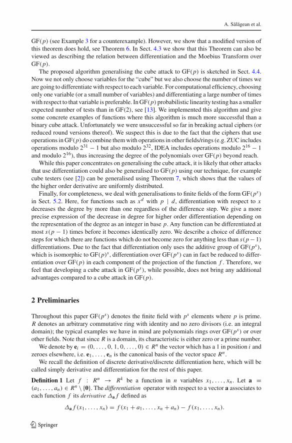
GF(p) (see Example 3 for a counterexample). However, we show that a modified version ofthis theorem does hold, see Theorem 6. In Sect. 4.3 we show that this Theorem can also beviewed as describing the relation between differentiation and the Moebius Transform overGF(p).
The proposed algorithm generalising the cube attack to GF(p) is sketched in Sect. 4.4.Now we not only choose variables for the “cube” but we also choose the number of times weare going to differentiatewith respect to each variable. For computational efficiency, choosingonly one variable (or a small number of variables) and differentiating a large number of timeswith respect to that variable is preferable. InGF(p) probabilistic linearity testing has a smallerexpected number of tests than in GF(2), see [13]. We implemented this algorithm and givesome concrete examples of functions where this algorithm is much more successful than abinary cube attack. Unfortunately we were unsuccessful so far in breaking actual ciphers (orreduced round versions thereof). We suspect this is due to the fact that the ciphers that useoperations inGF(p) do combine themwith operations in other fields/rings (e.g. ZUC includesoperations modulo 231 − 1 but also modulo 232, IDEA includes operations modulo 216 − 1and modulo 216), thus increasing the degree of the polynomials over GF(p) beyond reach.
While this paper concentrates on generalising the cube attack, it is likely that other attacksthat use differentiation could also be generalised to GF(p) using our technique, for examplecube testers (see [2]) can be generalised using Theorem 7, which shows that the values ofthe higher order derivative are uniformly distributed.
Finally, for completeness, we deal with generalisations to finite fields of the form GF(ps)in Sect. 5.2. Here, for functions such as xd with p | d , differentiation with respect to xdecreases the degree by more than one regardless of the difference step. We give a moreprecise expression of the decrease in degree for higher order differentiation depending onthe representation of the degree as an integer in base p. Any function can be differentiated atmost s(p − 1) times before it becomes identically zero. We describe a choice of differencesteps for which there are functions which do not become zero for anything less than s(p−1)differentiations. Due to the fact that differentiation only uses the additive group of GF(ps),which is isomorphic to GF(p)s , differentiation over GF(ps) can in fact be reduced to differ-entiation over GF(p) in each component of the projection of the function f . Therefore, wefeel that developing a cube attack in GF(ps), while possible, does not bring any additionaladvantages compared to a cube attack in GF(p).
2 Preliminaries
Throughout this paper GF(ps) denotes the finite field with ps elements where p is prime.R denotes an arbitrary commutative ring with identity and no zero divisors (i.e. an integraldomain); the typical examples we have in mind are polynomials rings over GF(ps) or overother fields. Note that since R is a domain, its characteristic is either zero or a prime number.
We denote by ei = (0, . . . , 0, 1, 0, . . . , 0) ∈ Rn the vector which has a 1 in position i andzeroes elsewhere, i.e. e1, . . . , en is the canonical basis of the vector space Rn .
We recall the definition of discrete derivative/discrete differentiation here, which will becalled simply derivative and differentiation for the rest of this paper.
Definition 1 Let f : Rn → Rk be a function in n variables x1, . . . , xn . Let a =(a1, . . . , an) ∈ Rn \ {0}. The differentiation operator with respect to a vector a associates toeach function f its derivative Δa f defined as
Δa f (x1, . . . , xn) = f (x1 + a1, . . . , xn + an) − f (x1, . . . , xn).
123
Higher order differentiation over finite fields
Denoting x = (x1, . . . , xn) we can also write Δa f (x) = f (x + a) − f (x).For the particular case of a = hei for some 1 ≤ i ≤ n and h ∈ R\{0}, wewill callΔhei the
differentiation operator with respect to the variable xi with step h, or simply differentiationwith respect to the variable xi if h = 1 or if h is clear from the context. We will use theabbreviation “w.r.t. xi” for “with respect to xi”.
Remark 1 Note that the discrete derivativewith respect to a variable x should not be confusedwith the formal derivative with respect to x . For example, for the function f : GF(5) →GF(5), f (x) = x3, the discrete derivative is 3x2 + 3x + 1 whereas the formal derivative is3x2. While the degree and leading coefficient are the same for both the discrete derivativeand formal derivative, in the context of “black box” functions it is preferable to work withthe discrete derivative: to evaluate the discrete derivative at one point we only need twoevaluations of the original function (i.e. two calls to the black box), whereas to evaluate theformal derivative we typically require evaluations of the original function at most points inits domain, which would be as costly as a full interpolation of the “black box” function. Thetwo notions of discrete derivative and formal derivative coincide for polynomials of degree atmost one in x , so in particular for all functions over GF(2), as they can always be representedas polynomial functions of degree at most one in each variable.
Remark 2 For defining the (discrete) differentiation operator, we do not actually need toworkover a ring R, a commutative group (using additive notation for convenience) is sufficient.Here we used a ring due to our application to finite fields, and also due to some of thetechniques involving polynomials.
The differentiation operator is a linear operator; composition of such operators is com-mutative and associative. Repeated application of the operator (also called higher orderdifferentiation or higher order derivative in [16]) will be denoted by
Δ(m)a1,...,am f = Δa1Δa2 . . . Δam f (1)
where a1, . . . , am ∈ Rn are not necessarily distinct. An explicit formula can be obtainedeasily from Definition 1 by induction (see [16, Proposition 3]):
Proposition 1 Let f : Rn → Rk be a function in n variables x1, . . . , xn. Let a1, . . . , am ∈Rn \ {0} not necessarily distinct. Then
Δ(m)a1,...,am f (x) =
m∑
j=0
(−1)m− j∑
{i1,...,i j }⊆{1,...,m}f(x + ai1 + · · · + aij
)
=∑
b∈{0,1}m(−1)m−w(b) f
(x + b1a1 + · · · + x + bmam
)
where w( ) denotes the Hamming weight, i.e. the number of non-zero entries of a vector.
In particular, when we differentiate a function w.r.t. one variable repeatedly, with alldifferentiation steps equal to 1 we obtain the following formula, well known in the contextof finite differences:
Δ(m)e1,...,e1 f (x1, . . . , xn) =
m∑
i=0
(−1)m−i(m
i
)f (x1 + i, x2, . . . , xn). (2)
While the derivative can be defined for any function, in the sequel we will concentrate onpolynomial functions. We will denote by degxi ( f ) the degree of f in the variable xi . Thetotal degree will be denoted deg( f ), with the usual convention of deg(0) = −∞.
123
A. Salagean et al.
Proposition 2 ([16, Proposition 2]) Let f : Rn → R be a polynomial function in n variablesand a ∈ Rn \ {0}. Then deg(Δa f ) ≤ deg( f ) − 1.
Differentiating with respect to one variable decreases the degree in that variable by at leastone:
Proposition 3 Let f : Rn → R be a polynomial function. Let h, h1, . . . , hm ∈ R \ {0}and i ∈ {1, . . . , n}. If degxi ( f ) = 0 then Δhei f (x1, . . . , xn) ≡ 0. If degxi ( f ) > 0 then
degxi (Δhei f ) ≤ degxi ( f ) − 1. Consequently degxi (Δ(m)h1ei,...,hmei
f ) ≤ degxi ( f ) − m.
Recall that for integers d, k1, k2, . . . , km such that∑m
i=1 ki = d and ki ≥ 0 the multino-mial coefficient is defined as:
(d
k1, k2, . . . , km
)= d!
k1!k2! · · · km ! ,
generalising binomials coefficients, as(dk
) = ( dk,d−k
).
Next we examine the effect of higher order differentiation on univariate monomials. Thisresult is straightforward and probably known but we could not find a reference sowe includeda proof for completeness; the general formula for univariate polynomials can be obtainedusing the linearity of the Δ operator.
Theorem 1 Let f : R → R defined by f (x) = xd and let h1, . . . , hm ∈ R \ {0}. Then
Δ(m)h1e1,...,hme1
xd =d∑
j=m
(d
j
)⎛
⎜⎜⎝∑
(k1,...,km )∈{1,2,..., j−m+1}mk1+...+km= j
(j
k1, . . . , km
)hk11 · · · hkmm
⎞
⎟⎟⎠ xd− j
Proof Induction onm. Form = 1we haveΔh1e1xd = (x+h1)d−xd = ∑d
j=1
(dj
)h j1x
d− j =∑d
j=1
( dj,d− j
)h j1x
d− j and the statement is verified.Now let us assume the statement holds for a given m and we prove it for m + 1.
Δ(m+1)h1e1,...,hm+1e1
xd = Δhm+1e1Δ(m)h1e1,...,hme1
xd
=d∑
j=m
(d
j
)⎛
⎜⎜⎝∑
(k1,...,km )∈{1,2,..., j−m+1}mk1+···+km= j
(j
k1, . . . , km
)hk11 · · · hkmm
⎞
⎟⎟⎠((x + hm+1)
d− j −xd− j )
=d∑
j=m
(d
j
)⎛
⎜⎜⎝∑
(k1,...,km )∈{1,2,..., j−m+1}mk1+···+km= j
(j
k1, . . . , km
)hk11 · · · hkmm
⎞
⎟⎟⎠
×⎛
⎝d− j∑
km+1=1
(d − j
km+1
)hkm+1m+1 x
d− j−km+1
⎞
⎠
=d∑
j ′=m+1
(d
j ′
)⎛
⎜⎜⎜⎝∑
(k1,...,km+1)∈{1,2,..., j ′−m}m+1
k1+···+km+1= j ′
(j ′
k1, . . . , km+1
)hk11 · · · hkm+1
m+1
⎞
⎟⎟⎟⎠ xd− j ′ .
123
Higher order differentiation over finite fields
In the last line we denoted j ′ = j + km+1 and used the identity:(d
j
)(j
k1, . . . , km
)(d − j
km+1
)=
(d
j ′
)(j ′
k1, . . . , km+1
).
�Recall that in a finite field GF(ps) we have a ps = a for all elements a. Hence, while
(formal) polynomials over GF(ps) could have any degree in each variable, when we talkabout the associated polynomial function, there will always be a unique polynomial ofdegree at most ps − 1 in each variable which defines the same polynomial function. In otherwords we are working in the quotient ring GF(ps)[x1, . . . , xn]/〈x ps
1 − x1, . . . xpsn − xn〉, and
we use as representative of each class the unique polynomial which has degree at most ps −1in each variable.
Moreover, all functions in n variables over a finite field can bewritten in Algebraic NormalForm (ANF) i.e. as polynomial functions of n variables. To summarise, each function in nvariables over GF(ps) can be uniquely expressed as a polynomial function defined by apolynomial in GF(ps)[x1, . . . , xn] of degree at most ps − 1 in each variable.
The transform that associates to each function f : GF(p)n → GF(p) the coefficients ofits ANF is called the Moebius transform or Reed–Muller transform. More precisely, usingthe usual representation of GF(p) as {0, 1, . . . , p − 1}, the transform of f is a functionf M : GF(p)n → GF(p) with f M (y1, . . . , yn) defined as being equal to the coefficient ofx y11 · · · x ynn in the ANF of f . We define a partial order on GF(p)n as a � b iff ai ≤ bi forall i = 1, . . . , n (the order ≤ on GF(p) = {0, 1, . . . , p − 1} being the usual order on theintegers). In the binary case, the Moebius transform of f can be obtained from the truth tableof f using the following result (see for example [19, Chapter 13, Theorem 1]):
Theorem 2 Let f : GF(2)n → GF(2). With the notations above,
f M (y) =∑
a�y
f (a). (3)
Note that using the Theorem above and Proposition 1 we also have that f M (y) =Δ
(m)ei1 ,...,eim f (0) where i1, . . . im are the positions of the non-zero elements of y. An effi-
cient algorithm for computing the truth table of f M from the truth table of f is given forexample in [12, Algorithm 9.6]. The algorithm has O(n2n) complexity and works in-place(i.e. no significant additional memory needed). For computing f M over GF(p) with p > 2,Theorem 2 does not hold; however f M can be computed by the an in-place algorithm givenin [12, Algorithm 9.9] with npn−1(p − 1)2 operations, hence O(npn+1) complexity.
3 The cube/AIDA attack
3.1 Binary cube/AIDA attack
We recall the classical cube/AIDA attacks (see [5] and [21]) and their interpretation in theframework of higher order derivatives (see [7,14]). Throughout this subsection we work inthe binary field GF(2).
The next definitions are taken from [5]: “Any subset I of size k defines a k dimensionalBoolean cube CI of 2k vectors in which we assign all the possible combinations of 0/1values to variables in I and leave all the other variables undetermined. Any vector v ∈ CI
123
A. Salagean et al.
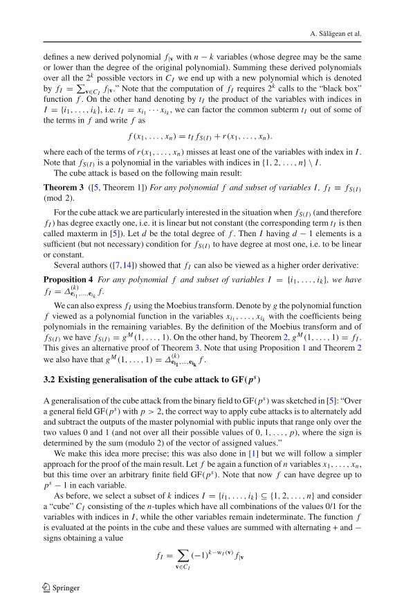
defines a new derived polynomial f|v with n − k variables (whose degree may be the sameor lower than the degree of the original polynomial). Summing these derived polynomialsover all the 2k possible vectors in CI we end up with a new polynomial which is denotedby f I = ∑
v∈CIf|v.” Note that the computation of f I requires 2k calls to the “black box”
function f . On the other hand denoting by tI the product of the variables with indices inI = {i1, . . . , ik}, i.e. tI = xi1 · · · xik , we can factor the common subterm tI out of some ofthe terms in f and write f as
f (x1, . . . , xn) = tI fS(I ) + r(x1, . . . , xn).
where each of the terms of r(x1, . . . , xn) misses at least one of the variables with index in I .Note that fS(I ) is a polynomial in the variables with indices in {1, 2, . . . , n} \ I .
The cube attack is based on the following main result:
Theorem 3 ([5, Theorem 1]) For any polynomial f and subset of variables I , f I ≡ fS(I )
(mod 2).
For the cube attack we are particularly interested in the situation when fS(I ) (and thereforef I ) has degree exactly one, i.e. it is linear but not constant (the corresponding term tI is thencalled maxterm in [5]). Let d be the total degree of f . Then I having d − 1 elements is asufficient (but not necessary) condition for fS(I ) to have degree at most one, i.e. to be linearor constant.
Several authors ([7,14]) showed that f I can also be viewed as a higher order derivative:
Proposition 4 For any polynomial f and subset of variables I = {i1, . . . , ik}, we havef I = Δ
(k)ei1 ,...,eik
f.
We can also express f I using theMoebius transform. Denote by g the polynomial functionf viewed as a polynomial function in the variables xi1 , . . . , xik with the coefficients beingpolynomials in the remaining variables. By the definition of the Moebius transform and offS(I ) we have fS(I ) = gM (1, . . . , 1). On the other hand, by Theorem 2, gM (1, . . . , 1) = f I .This gives an alternative proof of Theorem 3. Note that using Proposition 1 and Theorem 2we also have that gM (1, . . . , 1) = Δ
(k)ei1 ,...,eik
f .
3.2 Existing generalisation of the cube attack to GF( ps)
Ageneralisation of the cube attack from the binary field to GF(ps)was sketched in [5]: “Overa general field GF(ps) with p > 2, the correct way to apply cube attacks is to alternately addand subtract the outputs of the master polynomial with public inputs that range only over thetwo values 0 and 1 (and not over all their possible values of 0, 1, . . . , p), where the sign isdetermined by the sum (modulo 2) of the vector of assigned values.”
We make this idea more precise; this was also done in [1] but we will follow a simplerapproach for the proof of the main result. Let f be again a function of n variables x1, . . . , xn ,but this time over an arbitrary finite field GF(ps). Note that now f can have degree up tops − 1 in each variable.
As before, we select a subset of k indices I = {i1, . . . , ik} ⊆ {1, 2, . . . , n} and considera “cube” CI consisting of the n-tuples which have all combinations of the values 0/1 for thevariables with indices in I , while the other variables remain indeterminate. The function fis evaluated at the points in the cube and these values are summed with alternating + and −signs obtaining a value
f I =∑
v∈CI
(−1)k−wI (v) f|v
123
Higher order differentiation over finite fields
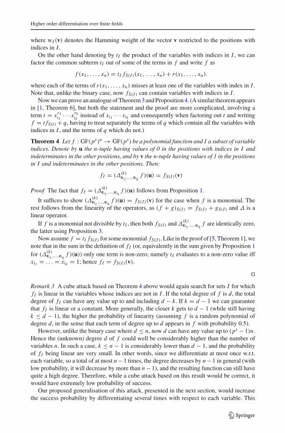
where wI (v) denotes the Hamming weight of the vector v restricted to the positions withindices in I .
On the other hand denoting by tI the product of the variables with indices in I , we canfactor the common subterm tI out of some of the terms in f and write f as
f (x1, . . . , xn) = tI fS(I )(x1, . . . , xn) + r(x1, . . . , xn).
where each of the terms of r(x1, . . . , xn) misses at least one of the variables with index in I .Note that, unlike the binary case, now fS(I ) can contain variables with indices in I .
Nowwecanprove an analogueofTheorem3andProposition 4. (A similar theoremappearsin [1, Theorem 6], but both the statement and the proof are more complicated, involving aterm t = xr1i1 · · · xrkik instead of xi1 · · · xik and consequently when factoring out t and writingf = t fS(t) + q , having to treat separately the terms of q which contain all the variables withindices in I , and the terms of q which do not.)
Theorem 4 Let f : GF(ps)n → GF(ps) be a polynomial function and I a subset of variableindices. Denote by u the n-tuple having values of 0 in the positions with indices in I andindeterminates in the other positions, and by v the n-tuple having values of 1 in the positionsin I and indeterminates in the other positions. Then:
f I = (Δ(k)ei1 ,...,eik
f )(u) = fS(I )(v)
Proof The fact that f I = (Δ(k)ei1 ,...,eik
f )(u) follows from Proposition 1.
It suffices to show (Δ(k)ei1 ,...,eik
f )(u) = fS(I )(v) for the case when f is a monomial. Therest follows from the linearity of the operators, as ( f + g)S(I ) = fS(I ) + gS(I ) and Δ is alinear operator.
If f is a monomial not divisible by tI , then both fS(I ) andΔ(k)ei1 ,...,eik
f are identically zero,the latter using Proposition 3.
Nowassume f = tI fS(I ) for somemonomial fS(I ). Like in the proof of [5, Theorem1],wenote that in the sum in the definition of f I (or, equivalently in the sum given by Proposition 1for (Δ
(k)ei1 ,...,eik
f )(u)) only one term is non-zero; namely tI evaluates to a non-zero value iffxi1 = . . . = xik = 1; hence f I = fS(I )(v).
�Remark 3 A cube attack based on Theorem 4 above would again search for sets I for whichf I is linear in the variables whose indices are not in I . If the total degree of f is d , the totaldegree of f I can have any value up to and including d − k. If k = d − 1 we can guaranteethat f I is linear or a constant. More generally, the closer k gets to d − 1 (while still havingk ≤ d − 1), the higher the probability of linearity (assuming f is a random polynomial ofdegree d , in the sense that each term of degree up to d appears in f with probability 0.5).
However, unlike the binary case where d ≤ n, now d can have any value up to (ps − 1)n.Hence the (unknown) degree d of f could well be considerably higher than the number ofvariables n. In such a case, k ≤ n − 1 is considerably lower than d − 1, and the probabilityof f I being linear are very small. In other words, since we differentiate at most once w.r.t.each variable, so a total of at most n−1 times, the degree decreases by n−1 in general (withlow probability, it will decrease by more than n−1), and the resulting function can still havequite a high degree. Therefore, while a cube attack based on this result would be correct, itwould have extremely low probability of success.
Our proposed generalisation of this attack, presented in the next section, would increasethe success probability by differentiating several times with respect to each variable. This
123

A. Salagean et al.
will result in a greater decrease of the degree, thus improving the probability of reaching alinear result.
4 Generalisations to GF( p)
4.1 Differentiation in GF( p)
Differentiation with respect to a variable decreases the degree in that variable by at least one.In the binary case, the degree of a polynomial function in each variable is at most one, so wecan only differentiate once w.r.t. each variable; a second differentiation will trivially producethe zero function. In GF(p) the degree in each variable is up to p − 1. We can thereforeconsider differentiating several times (and possibly using different difference steps) withrespect to each variable. We first show that any polynomial of degree di in a variable xi canbe differentiated mi times w.r.t. xi , for any mi ≤ di (and using any collection of non-zerodifference steps) and the degree decreases by exactlymi . Hence we can differentiate di timeswithout the result becoming identically zero.
Proposition 5 Let f : GF(p)n → GF(p) and 1 ≤ m1 ≤ degx1( f ) < p. Let h1, . . . , hm1 ∈GF(p) \ {0}. Then
degx1(Δ
(m1)h1e1,...,hm1 e1
f) = degx1( f ) − m1.
Proof We first assume f = xd11 , and we use Theorem 1. The coefficient of xd1−m11 equals
(d1m1
)(m1
1, 1, . . . , 1
)h1 · · · hm1 = d1!
(d1 − m1)!h1 · · · hm1 .
Since d1 = degx1( f ) < p, we have thatd1!
(d1 − m1)! , as an integer, is not divisible by p, so
it is non-zero in GF(p).When f is an arbitrary polynomial, we can write it as f = ∑d1
i=0 gi xi1 with gi ∈
GF(p)[x2, . . . , xn]. We have degx1(Δ(m1)h1e1,...,hm1 e1
gi xi1) = i − m1 and since the derivative
of each gi xi1 has a different degree in x1 their leading monomials cannot cancel out so
degx1(Δ(m1)h1e1,...,hm1 e1
gi xi1) = d1 − m1.
�Example 1 Let f (x1, x2, x3, x4) = x51 x2 + x41 x3x4 + x64 be a polynomial with coefficientsin GF(31). We choose the variable x1 and differentiate repeatedly w.r.t. x1, always withdifference step equal to one. Differentiating once w.r.t. x1 we obtain:
Δe1 f (x1, x2, x3, x4) = x41 (5x2) + x31 (10x2 + 4x3x4) + x21 (10x2 + 6x3x4)
+x1(5x2 + 4x3x4) + x2 + x3x4
Differentiating again w.r.t. x1 we obtain:
Δ(2)e1,e1 f (x1, x2, x3, x4) = x31 (20x2) + x21 (29x2 + 12x3x4)
+x1(8x2 + 24x3x4) + 30x2 + 14x3x4
Finally, if we differentiate a total of 5 times we obtain:
Δ(5)e1,...,e1 f (x1, x2, x3, x4) = 5!x2 = 27x2.
123
Higher order differentiation over finite fields
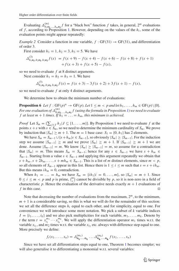
Evaluating Δ(m)h1e1,...,hme1
f for a “black box” function f takes, in general, 2m evaluationsof f , according to Proposition 1. However, depending on the values of the hi , some of theevaluation points might appear repeatedly:
Example 2 Consider a function in one variable, f : GF(31) → GF(31), and differentiationof order 3.
First consider h1 = 1, h2 = 3, h3 = 5. We have
Δ(3)h1e1,h2e1,h3e1
f (x) = f (x + 9) − f (x + 4) − f (x + 6) − f (x + 8) + f (x + 1)
+ f (x + 3) + f (x + 5) − f (x),
so we need to evaluate f at 8 distinct arguments.Next consider h1 = h2 = h3 = 1. We have
Δ(3)h1e1,h2e1,h3e1
f (x) = f (x + 3) − 3 f (x + 2) + 3 f (x + 1) − f (x),
so we need to evaluate f at only 4 distinct arguments.
We determine how to obtain the minimum number of evaluations:
Proposition 6 Let f : GF(p)n → GF(p). Let 1 ≤ m < p and let h1, . . . , hm ∈ GF(p)\{0}.For one evaluation ofΔ(m)
h1e1,...,hme1f (using the formula in Proposition 1) we need to evaluate
f at least m + 1 times. If h1 = . . . = hm, this minimum is achieved.
Proof Let Sm = {∑ j∈J h j |J ⊆ {1, . . . ,m}}. By Proposition 1 we need to evaluate f at thepoints x + s with s ∈ Sm , so we need to determine the minimum cardinality of Sm . We proveby induction that |Sm | ≥ m + 1. The m = 1 base case: S1 = {0, h1} has 2 elements.
We have Sm = Sm−1∪{s+hm |s ∈ Sm−1}, so obviously |Sm | ≥ |Sm−1|. For the inductionstep we assume |Sm−1| ≥ m and we prove |Sm | ≥ m + 1. If |Sm−1| ≥ m + 1 we aredone. Assume |Sm−1| = m. We know |Sm | ≥ |Sm−1| = m, so assume for a contradictionthat |Sm | = m. This means Sm = Sm−1; hence for any s ∈ Sm−1 we have s + hm ∈Sm−1. Starting from a value s ∈ Sm−1 and applying this argument repeatedly we obtain thats + hm, s + 2hm, . . . , s + mhm ∈ Sm−1. This is a list of m distinct elements, since m < p,so all elements of Sm−1 appear in this list. Hence there is 1 ≤ i ≤ m such that s = s + ihm .But this means ihm = 0, contradiction.
When h1 = . . . = hm we have Sm = {ih1|i = 0, . . . ,m}, so |Sm | = m + 1. Since0 ≤ i ≤ m < p and p is prime,
(mi
)cannot be divisible by p, so it is non-zero in a field of
characteristic p. Hence the evaluation of the derivative needs exactly m + 1 evaluations off in this case. �Note that decreasing the number of evaluations from the maximum, 2m , to the minimum,
m + 1 is a considerable saving, so this is what we will do for the remainder of this section:we set all the difference steps hi equal to each other, and for simplicity, equal to one. Forconvenience we will introduce some more notation. We pick a subset of k variable indicesI = {i1, . . . , ik} and we also pick multiplicities for each variable, m1, . . . ,mk . Denote byt the term t = xm1
i1· · · xmk
ik. We will apply the differentiation operator m1 times w.r.t. the
variable xi1 , andm2 times w.r.t. the variable xi2 etc. always with difference step equal to one.More precisely we define:
ft (x1, . . . , xn) = Δ(m1)ei1 ,...,ei1
. . . Δ(mk )eik ,...,eik
f (x1, . . . , xn)
Since we have set all differentiation steps equal to one, Theorem 1 becomes simpler; wewill also generalise it to differentiating a monomial w.r.t. several variables:
123
A. Salagean et al.
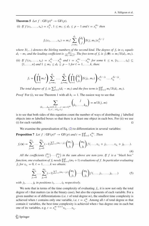
Theorem 5 Let f : GF(p)n → GF(p).
(i) If f (x1, . . . , xn) = xd11 , 1 ≤ m1 ≤ d1 ≤ p − 1 and t = xm11 then
ft (x1, . . . , xn) = m1!d1∑
j=m1
(d1j
)S( j,m1)x
d1− j1
where S(., .) denotes the Stirling numbers of the second kind. The degree of ft in x1 equalsd1 −m1 and the leading coefficient is
d1!(d1−m1)! . The free term of ft is ft (0) = m1!S(d1,m1).
(ii) If f (x1, . . . , xn) = xd1i1 · · · xdkik and t = xm1i1
· · · xmkik
for some k ≤ n, {i1, . . . , ik} ⊆{1, . . . , n} and 1 ≤ m� ≤ d� ≤ p − 1 for � = 1, . . . , k, then:
ft =(
k∏
�=1
m�!)
d1∑
j1=m1
. . .
dk∑
jk=mk
(k∏
�=1
(d�
j�
)S( j�,m�)
)xd1− j1i1
. . . xdk− jkik
.
The total degree of ft is∑k
�=1(d� − m�) and the free term is∏k
�=1 m�!S(d�,m�).
Proof For (i), we use Theorem 1 with all hi = 1. The easiest way to see that
∑
(k1,...,km )∈{1,2,..., j−m+1}mk1+...+km= j
(j
k1, . . . , km
)= m!S( j,m)
is to see that both sides of this equation count the number of ways of distributing j labelledobjects into m labelled boxes so that there is at least one object in each box. For (ii) we use(i) for each variable. �
We examine the generalisation of Eq. (2) to differentiation in several variables:
Proposition 7 Let f : GF(p)n → GF(p) and t = ∏k�=1 x
m�
i�. Then
ft (x) =m1∑
j1=0
. . .
mk∑
jk=0
(−1)∑k
�=1(m�− j�)(m1
j1
)· · ·
(mk
jk
)f (. . . , xi1 + j1, . . . , xik + jk, . . .).
(4)All the coefficients
(m1j1
) · · · (mkjk
)in the sum above are non-zero. If f is a “black box”
function, one evaluation of ft needs∏k
�=1(m� +1) evaluations of f . In particular evaluatingft for xi� = 0, � = 1, . . . , k we obtain:
m1∑
j1=0
. . .
mk∑
jk=0
(−1)∑k
�=1(m�− j�)(m1
j1
)· · ·
(mk
jk
)f (. . . , j1, . . . , jk, . . .) (5)
with j1, . . . , jk in positions i1, . . . , ik respectively.
We note that in terms of the time complexity of evaluating ft , it is now not only the totaldegree of t that matters (as in the binary case), but also the exponents of each variable. For agiven number m of differentiations (i.e. t of total degree m), the smallest time complexity isachieved when t contains only one variable, i.e. t = xmi1 . Among all t of total degree m thatcontain k variables, the best time complexity is achieved when t has degree one in each butone of its variables, e.g. t = xm−k+1
i1xi2 . . . xik .
123
Higher order differentiation over finite fields
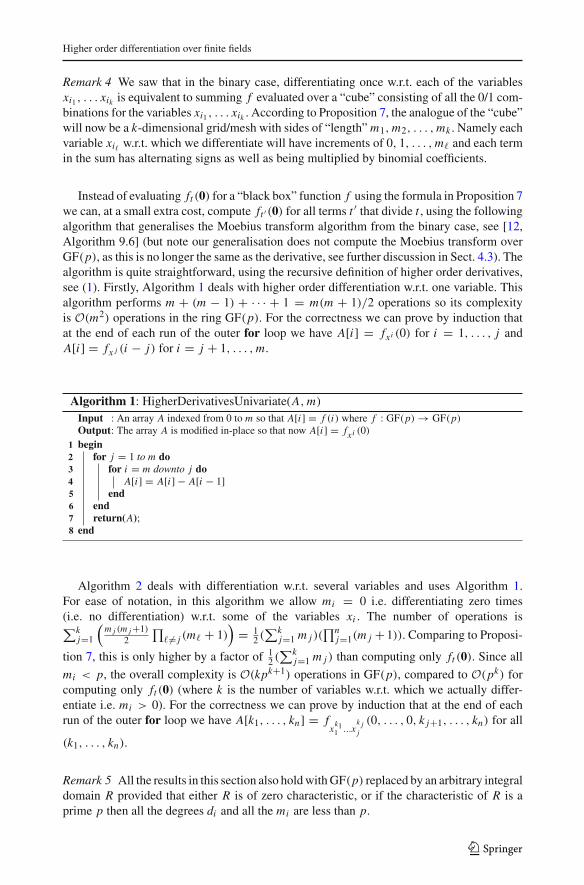
Remark 4 We saw that in the binary case, differentiating once w.r.t. each of the variablesxi1 , . . . xik is equivalent to summing f evaluated over a “cube” consisting of all the 0/1 com-binations for the variables xi1 , . . . xik . According to Proposition 7, the analogue of the “cube”will now be a k-dimensional grid/mesh with sides of “length”m1,m2, . . . ,mk . Namely eachvariable xi� w.r.t. which we differentiate will have increments of 0, 1, . . . ,m� and each termin the sum has alternating signs as well as being multiplied by binomial coefficients.
Instead of evaluating ft (0) for a “black box” function f using the formula in Proposition 7we can, at a small extra cost, compute ft ′(0) for all terms t ′ that divide t , using the followingalgorithm that generalises the Moebius transform algorithm from the binary case, see [12,Algorithm 9.6] (but note our generalisation does not compute the Moebius transform overGF(p), as this is no longer the same as the derivative, see further discussion in Sect. 4.3). Thealgorithm is quite straightforward, using the recursive definition of higher order derivatives,see (1). Firstly, Algorithm 1 deals with higher order differentiation w.r.t. one variable. Thisalgorithm performs m + (m − 1) + · · · + 1 = m(m + 1)/2 operations so its complexityis O(m2) operations in the ring GF(p). For the correctness we can prove by induction thatat the end of each run of the outer for loop we have A[i] = fxi (0) for i = 1, . . . , j andA[i] = fx j (i − j) for i = j + 1, . . . ,m.
Algorithm 1: HigherDerivativesUnivariate(A,m)Input : An array A indexed from 0 to m so that A[i] = f (i) where f : GF(p) → GF(p)Output: The array A is modified in-place so that now A[i] = fxi (0)begin1
for j = 1 to m do2for i = m downto j do3
A[i] = A[i] − A[i − 1]4end5
end6return(A);7
end8
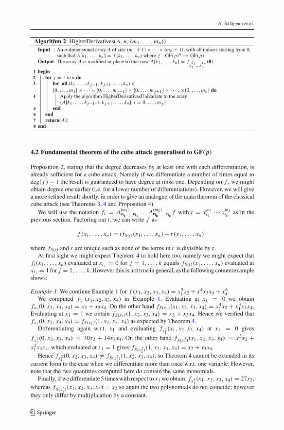
Algorithm 2 deals with differentiation w.r.t. several variables and uses Algorithm 1.For ease of notation, in this algorithm we allow mi = 0 i.e. differentiating zero times(i.e. no differentiation) w.r.t. some of the variables xi . The number of operations is∑k
j=1
(m j (m j+1)
2
∏��= j (m� + 1)
)= 1
2 (∑k
j=1 m j )(∏n
j=1(m j + 1)). Comparing to Proposi-
tion 7, this is only higher by a factor of 12 (
∑kj=1 m j ) than computing only ft (0). Since all
mi < p, the overall complexity is O(kpk+1) operations in GF(p), compared to O(pk) forcomputing only ft (0) (where k is the number of variables w.r.t. which we actually differ-entiate i.e. mi > 0). For the correctness we can prove by induction that at the end of eachrun of the outer for loop we have A[k1, . . . , kn] = f
xk11 ...x
k jj
(0, . . . , 0, k j+1, . . . , kn) for all
(k1, . . . , kn).
Remark 5 All the results in this section also holdwithGF(p) replaced by an arbitrary integraldomain R provided that either R is of zero characteristic, or if the characteristic of R is aprime p then all the degrees di and all the mi are less than p.
123
A. Salagean et al.
Algorithm 2: HigherDerivatives(A, n, (m1, . . . ,mn))Input : An n-dimensional array A of size (m1 + 1) × · · · × (mn + 1), with all indices starting from 0,
such that A[k1, . . . , kn ] = f (k1, . . . , kn) where f : GF(p)n → GF(p)Output: The array A is modified in-place so that now A[k1, . . . , kn ] = f
xk11 ...xknn
(0)
begin1for j = 1 to n do2
for all (k1, . . . , k j−1, k j+1, . . . , kn) ∈3
{0, . . . ,m1} × · · · × {0, . . . ,m j−1} × {0, . . . ,m j+1} × · · · , ×{0, . . . ,mn} doApply the algorithm HigherDerivativesUnivariate to the array4(A[k1, . . . , k j−1, i, k j+1, . . . , kn ], i = 0, . . . ,m j )
end5end6return(A);7
end8
4.2 Fundamental theorem of the cube attack generalised to GF( p)
Proposition 2, stating that the degree decreases by at least one with each differentiation, isalready sufficient for a cube attack. Namely if we differentiate a number of times equal todeg( f ) − 1 the result is guaranteed to have degree at most one. Depending on f , we mightobtain degree one earlier (i.e. for a lower number of differentiations). However, we will givea more refined result shortly, in order to give an analogue of the main theorem of the classicalcube attack (see Theorems 3, 4 and Proposition 4).
We will use the notation ft = Δ(m1)ei1 ,...,ei1
. . . Δ(mk )eik ,...,eik
f with t = xm1i1
· · · xmkik
as in theprevious section. Factoring out t , we can write f as
f (x1, . . . , xn) = t fS(t)(x1, . . . , xn) + r(x1, . . . , xn)
where fS(t) and r are unique such as none of the terms in r is divisible by t .At first sight we might expect Theorem 4 to hold here too, namely we might expect that
ft (x1, . . . , xn) evaluated at xi j = 0 for j = 1, . . . , k equals fS(t)(x1, . . . , xn) evaluated atxi j = 1 for j = 1, . . . , k. However this is not true in general, as the following counterexampleshows:
Example 3 We continue Example 1 for f (x1, x2, x3, x4) = x51 x2 + x41 x3x4 + x64 .We computed fx1(x1, x2, x3, x4) in Example 1. Evaluating at x1 = 0 we obtain
fx1(0, x2, x3, x4) = x2 + x3x4. On the other hand fS(x1)(x1, x2, x3, x4) = x41 x2 + x31 x3x4.Evaluating at x1 = 1 we obtain fS(x1)(1, x2, x3, x4) = x2 + x3x4. Hence we verified thatfx1(0, x2, x3, x4) = fS(x1)(1, x2, x3, x4) as expected by Theorem 4.Differentiating again w.r.t. x1 and evaluating fx21
(x1, x2, x3, x4) at x1 = 0 gives
fx21(0, x2, x3, x4) = 30x2 + 14x3x4. On the other hand fS(x21 )(x1, x2, x3, x4) = x31 x2 +
x21 x3x4, which evaluated at x1 = 1 gives fS(x21 )(1, x2, x3, x4) = x2 + x3x4.Hence fx21
(0, x2, x3, x4) �= fS(x21 )(1, x2, x3, x4), so Theorem 4 cannot be extended in itscurrent form to the case when we differentiate more than once w.r.t. one variable. However,note that the two quantities computed here do contain the same monomials.
Finally, if we differentiate 5 timeswith respect to x1 we obtain: fx51(x1, x2, x3, x4) = 27x2,
whereas fS(x51 )(x1, x2, x3, x4) = x2 so again the two polynomials do not coincide; howeverthey only differ by multiplication by a constant.
123
Higher order differentiation over finite fields
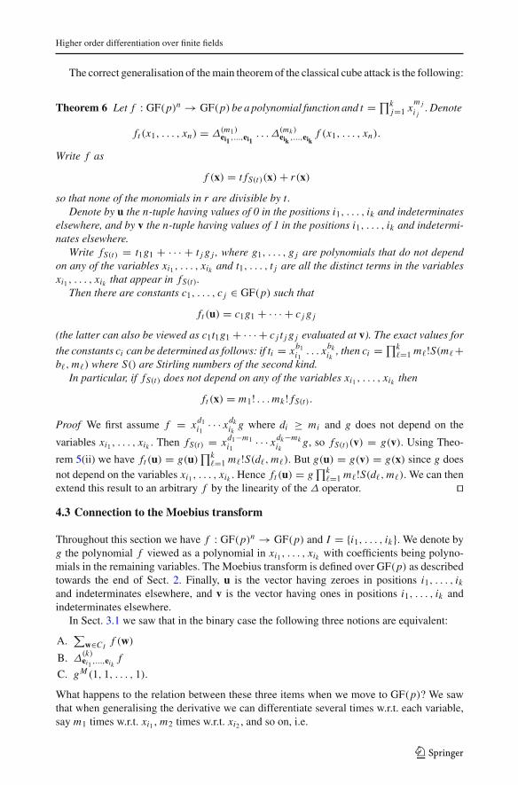
The correct generalisation of themain theorem of the classical cube attack is the following:
Theorem 6 Let f : GF(p)n → GF(p) be a polynomial function and t = ∏kj=1 x
m ji j
. Denote
ft (x1, . . . , xn) = Δ(m1)ei1 ,...,ei1
. . . Δ(mk )eik ,...,eik
f (x1, . . . , xn).
Write f as
f (x) = t fS(t)(x) + r(x)
so that none of the monomials in r are divisible by t.Denote by u the n-tuple having values of 0 in the positions i1, . . . , ik and indeterminates
elsewhere, and by v the n-tuple having values of 1 in the positions i1, . . . , ik and indetermi-nates elsewhere.
Write fS(t) = t1g1 + · · · + t j g j , where g1, . . . , g j are polynomials that do not dependon any of the variables xi1 , . . . , xik and t1, . . . , t j are all the distinct terms in the variablesxi1 , . . . , xik that appear in fS(t).
Then there are constants c1, . . . , c j ∈ GF(p) such that
ft (u) = c1g1 + · · · + c j g j
(the latter can also be viewed as c1t1g1 + · · · + c j t j g j evaluated at v). The exact values forthe constants ci can be determined as follows: if ti = xb1i1 . . . xbkik , then ci = ∏k
�=1 m�!S(m�+b�,m�) where S() are Stirling numbers of the second kind.
In particular, if fS(t) does not depend on any of the variables xi1 , . . . , xik then
ft (x) = m1! . . .mk ! fS(t).
Proof We first assume f = xd1i1 · · · xdkik g where di ≥ mi and g does not depend on the
variables xi1 , . . . , xik . Then fS(t) = xd1−m1i1
· · · xdk−mkik
g, so fS(t)(v) = g(v). Using Theo-
rem 5(ii) we have ft (u) = g(u)∏k
�=1 m�!S(d�,m�). But g(u) = g(v) = g(x) since g doesnot depend on the variables xi1 , . . . , xik . Hence ft (u) = g
∏k�=1 m�!S(d�,m�). We can then
extend this result to an arbitrary f by the linearity of the Δ operator. �4.3 Connection to the Moebius transform
Throughout this section we have f : GF(p)n → GF(p) and I = {i1, . . . , ik}. We denote byg the polynomial f viewed as a polynomial in xi1 , . . . , xik with coefficients being polyno-mials in the remaining variables. The Moebius transform is defined over GF(p) as describedtowards the end of Sect. 2. Finally, u is the vector having zeroes in positions i1, . . . , ikand indeterminates elsewhere, and v is the vector having ones in positions i1, . . . , ik andindeterminates elsewhere.
In Sect. 3.1 we saw that in the binary case the following three notions are equivalent:
A.∑
w∈CIf (w)
B. Δ(k)ei1 ,...,eik
f
C. gM (1, 1, . . . , 1).
What happens to the relation between these three items when we move to GF(p)? We sawthat when generalising the derivative we can differentiate several times w.r.t. each variable,say m1 times w.r.t. xi1 , m2 times w.r.t. xi2 , and so on, i.e.
123
A. Salagean et al.
B. Δ(m1)ei1 ,...,ei1
. . . Δ(mk )eik ,...,eik
f
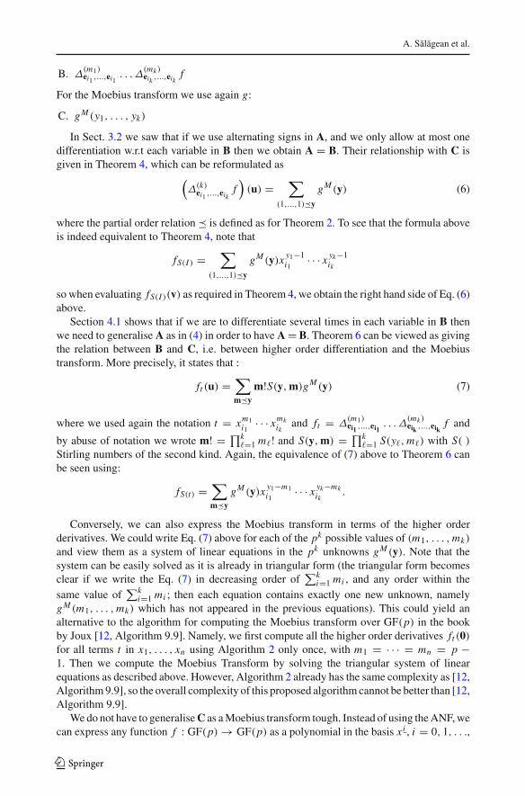
For the Moebius transform we use again g:
C. gM (y1, . . . , yk)
In Sect. 3.2 we saw that if we use alternating signs in A, and we only allow at most onedifferentiation w.r.t each variable in B then we obtain A = B. Their relationship with C isgiven in Theorem 4, which can be reformulated as
(Δ(k)
ei1 ,...,eikf)
(u) =∑
(1,...,1)�y
gM (y) (6)
where the partial order relation � is defined as for Theorem 2. To see that the formula aboveis indeed equivalent to Theorem 4, note that
fS(I ) =∑
(1,...,1)�y
gM (y)x y1−1i1
· · · x yk−1ik
so when evaluating fS(I )(v) as required in Theorem 4, we obtain the right hand side of Eq. (6)above.
Section 4.1 shows that if we are to differentiate several times in each variable in B thenwe need to generalise A as in (4) in order to have A = B. Theorem 6 can be viewed as givingthe relation between B and C, i.e. between higher order differentiation and the Moebiustransform. More precisely, it states that :
ft (u) =∑
m�y
m!S(y,m)gM (y) (7)
where we used again the notation t = xm1i1
· · · xmkik
and ft = Δ(m1)ei1 ,...,ei1
. . . Δ(mk )eik ,...,eik
f and
by abuse of notation we wrote m! = ∏k�=1 m�! and S(y,m) = ∏k
�=1 S(y�,m�) with S( )
Stirling numbers of the second kind. Again, the equivalence of (7) above to Theorem 6 canbe seen using:
fS(t) =∑
m�y
gM (y)x y1−m1i1
· · · x yk−mkik
.
Conversely, we can also express the Moebius transform in terms of the higher orderderivatives. We could write Eq. (7) above for each of the pk possible values of (m1, . . . ,mk)
and view them as a system of linear equations in the pk unknowns gM (y). Note that thesystem can be easily solved as it is already in triangular form (the triangular form becomesclear if we write the Eq. (7) in decreasing order of
∑ki=1 mi , and any order within the
same value of∑k
i=1 mi ; then each equation contains exactly one new unknown, namelygM (m1, . . . ,mk) which has not appeared in the previous equations). This could yield analternative to the algorithm for computing the Moebius transform over GF(p) in the bookby Joux [12, Algorithm 9.9]. Namely, we first compute all the higher order derivatives ft (0)for all terms t in x1, . . . , xn using Algorithm 2 only once, with m1 = · · · = mn = p −1. Then we compute the Moebius Transform by solving the triangular system of linearequations as described above. However, Algorithm 2 already has the same complexity as [12,Algorithm9.9], so the overall complexity of this proposed algorithmcannot be better than [12,Algorithm 9.9].
We do not have to generaliseC as aMoebius transform tough. Instead of using theANF,wecan express any function f : GF(p) → GF(p) as a polynomial in the basis xi , i = 0, 1, . . .,
123
Higher order differentiation over finite fields
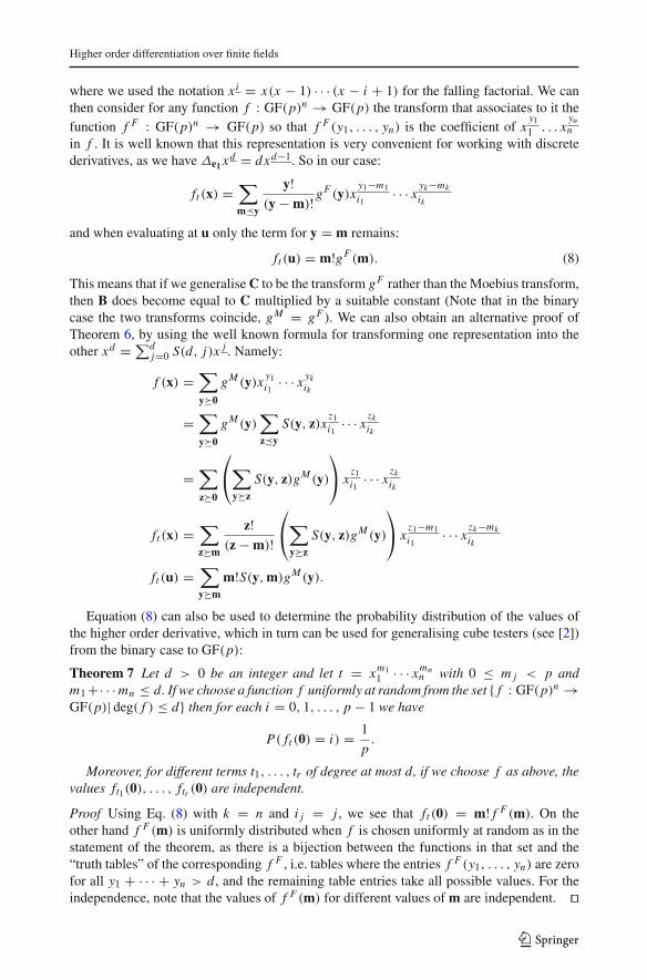
where we used the notation xi = x(x − 1) · · · (x − i + 1) for the falling factorial. We canthen consider for any function f : GF(p)n → GF(p) the transform that associates to it thefunction f F : GF(p)n → GF(p) so that f F (y1, . . . , yn) is the coefficient of x
y11 . . . x
ynn
in f . It is well known that this representation is very convenient for working with discretederivatives, as we have Δe1x
d = dxd−1. So in our case:
ft (x) =∑
m�y
y!(y − m)!g
F (y)xy1−m1
i1· · · x yk−mk
ik
and when evaluating at u only the term for y = m remains:
ft (u) = m!gF (m). (8)
This means that if we generaliseC to be the transform gF rather than the Moebius transform,then B does become equal to C multiplied by a suitable constant (Note that in the binarycase the two transforms coincide, gM = gF ). We can also obtain an alternative proof ofTheorem 6, by using the well known formula for transforming one representation into theother xd = ∑d
j=0 S(d, j)x j . Namely:
f (x) =∑
y�0
gM (y)x y1i1 · · · x ykik
=∑
y�0
gM (y)∑
z�y
S(y, z)xz1i1
· · · xzkik
=∑
z�0
⎛
⎝∑
y�z
S(y, z)gM (y)
⎞
⎠ xz1i1
· · · xzkik
ft (x) =∑
z�m
z!(z − m)!
⎛
⎝∑
y�z
S(y, z)gM (y)
⎞
⎠ xz1−m1
i1· · · xzk−mk
ik
ft (u) =∑
y�m
m!S(y,m)gM (y).
Equation (8) can also be used to determine the probability distribution of the values ofthe higher order derivative, which in turn can be used for generalising cube testers (see [2])from the binary case to GF(p):
Theorem 7 Let d > 0 be an integer and let t = xm11 · · · xmn
n with 0 ≤ m j < p andm1+· · ·mn ≤ d. If we choose a function f uniformly at random from the set { f : GF(p)n →GF(p)| deg( f ) ≤ d} then for each i = 0, 1, . . . , p − 1 we have
P( ft (0) = i) = 1
p.
Moreover, for different terms t1, . . . , tr of degree at most d, if we choose f as above, thevalues ft1(0), . . . , ftr (0) are independent.
Proof Using Eq. (8) with k = n and i j = j , we see that ft (0) = m! f F (m). On theother hand f F (m) is uniformly distributed when f is chosen uniformly at random as in thestatement of the theorem, as there is a bijection between the functions in that set and the“truth tables” of the corresponding f F , i.e. tables where the entries f F (y1, . . . , yn) are zerofor all y1 + · · · + yn > d , and the remaining table entries take all possible values. For theindependence, note that the values of f F (m) for different values ofm are independent. �
123
A. Salagean et al.
4.4 Proposed Algorithm for the cube attack in GF( p)
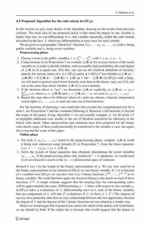
In this section we give more details of the algorithm, drawing on the results from previoussections. The main idea of our proposed attack is that when the degree in one variable ishigher than one, we can differentiate w.r.t. that variable repeatedly, unlike the cube attacksdescribed in the Sect. 3, which use differentiation at most once for each variable.
We are given a cryptographic “black box” function f (v1, . . . vm, x1, . . . , xn)with vi beingpublic variables and xi being secret variables.
Preprocessing phase
1. Choose a term in the public variables, t = vm1i1
· · · vmkik
, with 1 ≤ mi ≤ p − 1.2. Using formula (5) in Proposition 7 we evaluate ft (0, x) for several choices of the secret
variables x, in order to decide whether, with reasonably high probability, the total degreeof ft (0, x) in x equals one. (For this, one can use the textbook definition of linearity;namely, for various values of a, b ∈ GF(p) and y, z ∈ GF(p)n test whether a( ft (0, y)−ft (0, 0)) + b( ft (0, z) − ft (0, 0)) = ft (0, ay + bz) − ft (0, 0); in GF(p) with p large,we will need in general much fewer linearity tests than in the binary case, see [13]; onecan at the same time check whether ft (0, x) is non-constant).
3. If the decision above is “yes”, we determine ft (0, x) explicitly, as ft (0, x) = c0 +∑ni=1 ci xi where c0 = ft (0, 0) and ci = ft (0, ei ) − c0; we store (t, c0, c1, . . . , cn).
4. Repeat the steps above for different values of t until one obtains n linearly independentstored tuples (c1, . . . , cn), or until one runs out of time/memory.
For the heuristic of choosing t one could take into account the computational cost for aterm t , see Proposition 7 and the comment following it. However a full heuristic is beyondthe scope of this paper. Using Algorithm 2, we can actually compute ft ′ for all terms t ′|tat negligible additional cost, similar to the use of Moebius transform for efficiency in thebinary cube attack. Other optimisations and variations have been proposed for the binarycube attack; many of them could potentially be transferred to the modulo p case, but again,this is beyond the scope of this paper.
Online phase
1. For each (t, c0, c1, . . . , cn) stored in the preprocessing phase, compute ft (0, x) (withx being now unknown) using formula (5) in Proposition 7. Form the linear equation:c1x1 + · · · ,+cnxn + c0 = ft (0, x).
2. Solve the system of linear equations thus obtained, determining the secret variablesx1, . . . , xn . If the preprocessing phase only produced r < n equations, we would needto do an exhaustive search in the (n − r)-dimensional space of solutions.
Remark 6 Let � be the length of the binary representation of p. We can view each bit inthe binary representation of an element in GF(p) as one binary variable. If f is a functionof n variables over GF(p), we can also view it as � binary functions f (0), . . . , f (�−1) in �nbinary variables. We could therefore apply the classical (binary) cube attack on each of thesefunctions f ( j). A rough estimate suggests that the running time for corresponding cubeswill be approximately the same. (Differentiating p − 1 times with respect to one variable xiin GF(p) takes p evaluations of f ; differentiating once w.r.t. each of the binary variablesthat are components of xi will take 2� evaluations of f ; we have p ≈ 2�.) The chances ofsuccess on a particular cube bear no easy relationship between the two approaches, becausethe degree of f and the degrees of the � binary functions are not related in a simple way.
Hence wewould argue that in general one cannot tell which of the attacks will work better,so one should try both. If the cipher has a structure that would suggest that the degree as
123
Higher order differentiation over finite fields
polynomial over GF(p) is relatively low, then a cube attack over GF(p) should certainly bean approach to consider.
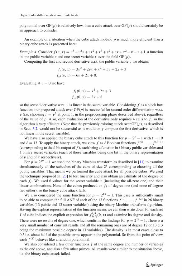
An example of a situation when the cube attack modulo p is much more efficient than abinary cube attack is presented here:
Example 4 Consider f (v, x) = v3 +v2x +vx2 + x3 +v2 +vx + x2 +v + x +1, a functionin one public variable v and one secret variable x over the field GF(p).
Computing the first and second derivative w.r.t. the public variable v we obtain:
fv(v, x) = 3v2 + 2vx + x2 + 5v + 2x + 3
fv2(v, x) = 6v + 2x + 8.
Evaluating at v = 0 we have:
fv(0, x) = x2 + 2x + 3
fv2(0, x) = 2x + 8
so the second derivative w.r.t. v is linear in the secret variable. Considering f as a black boxfunction, our proposed attack over GF(p) is successful for second order differentiation w.r.t.v (i.e. choosing t = v2 at point 1. in the preprocessing phase described above), regardlessof the value of p. Also, each evaluation of the derivative only requires 4 calls to f , so thealgorithm is very efficient. (Note that the previously existing attack over GF(p), as describedin Sect. 3.2, would not be successful as it would only compute the first derivative, which isnot linear in the secret variable).
We have also applied the binary cube attack to this function for p = 2� − 1 with � = 19and � = 13. To apply the binary attack, we view f as � Boolean functions f (0), . . . , f (�−1)
(corresponding to the �-bit output of f ), each being a function in � binary public variables and� binary secret variables (each of these variables being one bit in the binary representationof v and of x respectively).
For p = 219 − 1 we used the binary Moebius transform as described in [11] to examinesimultaneously all the subcubes of the cube of size 2� corresponding to choosing all thepublic variables. That means we performed the cube attack for all possible cubes. We usedthe technique proposed in [23] to test linearity and also obtain an estimate of the degree ofeach f I . We used 6 values for the secret variable x (including the all-zero one) and theirlinear combinations. None of the cubes produced an f I of degree one (and none of degreetwo either), so the binary cube attack fails.
We also considered the same function for p = 213 − 1. This case is sufficiently smallto be able to compute the full ANF of each of the 13 functions f (0), . . . , f (12) in 26 binaryvariables (13 public and 13 secret variables) using the binary Moebius transform algorithm.Having the explicit representation of the function means we can then write down for each setI of cube indices the explicit expression for f ( j)
S(I )(0, x) and examine its degree and density.
There were no results of degree one, which confirms the findings for p = 219 − 1. There is avery small number of constant results and all the remaining ones are of degree 12 or 13 (13being the maximum possible degree in 13 variables). The density is in most cases close to0.5 i.e. about half of the possible terms appear in the polynomial. So from this point of vieweach f ( j) behaves like a random polynomial.
We also considered a few other functions f of the same degree and number of variablesas the one above, and also a few other primes. All results were similar to the situation above,i.e. the binary cube attack failed.
123
A. Salagean et al.
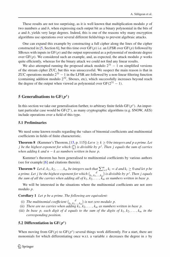
These results are not too surprising, as it is well known that multiplication modulo p oftwo numbers a and b, when expressing each output bit as a binary polynomial in the bits ofa and b, yields very large degrees. Indeed, this is one of the reasons why many encryptionalgorithms use operations over several different fields/rings to prevent algebraic attacks.
One can expand this example by constructing a full cipher along the lines of the cipherconstructed in [5, Section 6], but this time over GF(p) i.e. an LFSR over GF(p) followed bySBoxes with inputs in GF(p) and the output represented as a polynomial of moderate degreeover GF(p). We considered such an example, and, as expected, the attack modulo p worksquite efficiently, whereas for the binary attack we could not find any linear results.
We also attempted running the proposed attack modulo 231 − 1 on simplified versionsof the stream cipher ZUC, but this was unsuccessful. We suspect the main reason is that inZUC operations modulo 231 − 1 in the LFSR are followed by a non-linear filtering function(containing addition modulo 232, Sboxes, etc), which successfully increases beyond reachthe degree of the output when viewed as polynomial over GF(231 − 1).
5 Generalisations to GF( ps)
In this section we take our generalisation further, to arbitrary finite fields GF(ps). An impor-tant particular case would be GF(2s), as many cryptographic algorithms (e.g. SNOW, AES)include operations over a field of this type.
5.1 Preliminaries
We need some known results regarding the values of binomial coefficients and multinomialcoefficients in fields of finite characteristic.
Theorem 8 (Kummer’s Theorem, [15, p. 115]) Let n ≥ k ≥ 0 be integers and p a prime. Letj be the highest exponent for which
(nk
)is divisible by p j . Then j equals the sum of carries
when adding k and n − k as numbers written in base p.
Kummer’s theorem has been generalised to multinomial coefficients by various authors(see for example [6] and citations therein).
Theorem 9 Let d, k1, k2, . . . , km be integers such that∑m
i=1 ki = d and ki ≥ 0 and let p bea prime. Let j be the highest exponent for which
( dk1,k2,...,km
)is divisible by p j . Then j equals
the sum of all the carries when adding all of k1, k2, . . . , km as numbers written in base p.
We will be interested in the situations where the multinomial coefficients are not zeromodulo p.
Corollary 1 Let p be a prime. The following are equivalent:
(i) The multinomial coefficient( dk1,k2,...,km
)is not zero modulo p.
(ii) There are no carries when adding k1, k2, . . . , km as numbers written in base p.(iii) In base p, each digit of d equals to the sum of the digits of k1, k2, . . . , km in the
corresponding position.
5.2 Differentiation in GF( ps)
When moving from GF(p) to GF(ps) several things work differently. For a start, there aremonomials for which differentiating once w.r.t. a variable x decreases the degree in x by
123
Higher order differentiation over finite fields
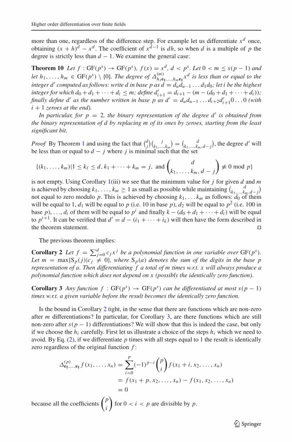
more than one, regardless of the difference step. For example let us differentiate xd once,obtaining (x + h)d − xd . The coefficient of xd−1 is dh, so when d is a multiple of p thedegree is strictly less than d − 1. We examine the general case:
Theorem 10 Let f : GF(ps) → GF(ps), f (x) = xd , d < ps . Let 0 < m ≤ s(p − 1) andlet h1, . . . , hm ∈ GF(ps) \ {0}. The degree of Δ
(m)h1e1,...,hme1
xd is less than or equal to theinteger d ′ computed as follows: write d in base p as d = dudu−1 . . . d1d0; let i be the highestinteger for which d0 + d1 + · · · + di ≤ m; define d ′
i+1 = di+1 − (m − (d0 + d1 + · · · + di ));finally define d ′ as the number written in base p as d ′ = dudu−1 . . . di+2d ′
i+10 . . . 0 (withi + 1 zeroes at the end).
In particular, for p = 2, the binary representation of the degree d ′ is obtained fromthe binary representation of d by replacing m of its ones by zeroes, starting from the leastsignificant bit.
Proof By Theorem 1 and using the fact that(dj
)( jk1,...,km
) = ( dk1,...,km ,d− j
), the degree d ′ will
be less than or equal to d − j where j is minimal such that the set
{(k1, . . . , km)|1 ≤ k� ≤ d, k1 + · · · + km = j, and
(d
k1, . . . , km, d − j
)�≡ 0 mod p}
is not empty. Using Corollary 1(iii) we see that the minimum value for j for given d and mis achieved by choosing k1, . . . , km ≥ 1 as small as possible while maintaining
( dk1,...,km ,d− j
)
not equal to zero modulo p. This is achieved by choosing k1, . . . km as follows: d0 of themwill be equal to 1, d1 will be equal to p (i.e. 10 in base p), d2 will be equal to p2 (i.e. 100 inbase p), . . ., di of them will be equal to pi and finally k − (d0 + d1 + · · · + di ) will be equalto pi+1. It can be verified that d ′ = d − (i1 + · · · + ik) will then have the form described inthe theorem statement. �
The previous theorem implies:
Corollary 2 Let f = ∑dj=0 c j x
j be a polynomial function in one variable over GF(ps).Let m = max{Sp( j)|c j �= 0}, where Sp(a) denotes the sum of the digits in the base prepresentation of a. Then differentiating f a total of m times w.r.t. x will always produce apolynomial function which does not depend on x (possibly the identically zero function).
Corollary 3 Any function f : GF(ps) → GF(ps) can be differentiated at most s(p − 1)times w.r.t. a given variable before the result becomes the identically zero function.
Is the bound in Corollary 2 tight, in the sense that there are functions which are non-zeroafter m differentiations? In particular, for Corollary 3, are there functions which are stillnon-zero after s(p − 1) differentiations? We will show that this is indeed the case, but onlyif we choose the hi carefully. First let us illustrate a choice of the steps hi which we need toavoid. By Eq. (2), if we differentiate p times with all steps equal to 1 the result is identicallyzero regardless of the original function f :
Δ(p)e1,...,e1 f (x1, . . . , xn) =
p∑
i=0
(−1)p−i(p
i
)f (x1 + i, x2, . . . , xn)
= f (x1 + p, x2, . . . , xn) − f (x1, x2, . . . , xn)
= 0
because all the coefficients
(p
i
)for 0 < i < p are divisible by p.
123
A. Salagean et al.
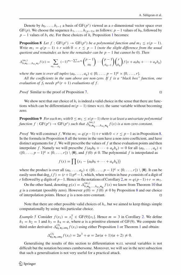
Denote by b0, . . . , bs−1 a basis of GF(ps) viewed as a s-dimensional vector space overGF(p). We choose the sequence h1, . . . , h(p−1)s as follows: p− 1 values of b0, followed byp − 1 values of b1 etc. For these choices of hi Proposition 1 becomes:
Proposition 8 Let f : GF(ps) → GF(ps) be a polynomial function and m1 ≤ s(p − 1).Write m1 = q(p − 1) + r with 0 < r ≤ p − 1 (note the slight difference from the usualquotient and remainder, as here the remainder can be p − 1 but cannot be 0). Then
Δ(m1)h1e1,...,hm1 e1
f (x) =∑
a0,...,aq
(−1)m1−∑qi=0 ai
(p − 1
a0
)· · ·
(p − 1
aq−1
)(r
aq
)f(x + a0b0 + · · · + aqbq
)
where the sum is over all tuples (a0, . . . , aq) ∈ {0, . . . , p − 1}q × {0, . . . , r}.All the coefficients in the sum above are non-zero. If f is a “black box” function, one
evaluation of ft needs pq(r + 1) evaluations of f .
Proof Similar to the proof of Proposition 7. �We show next that our choice of hi is indeed a valid choice in the sense that there are func-
tions which can be differentiated m(p − 1) times w.r.t. the same variable without becomingzero.
Proposition 9 For each m1 with 0 ≤ m1 ≤ s(p−1) there is at least a univariate polynomialfunction f : GF(ps) → GF(ps) such that Δ(m1)
h1ei1 ,...,hm1 ei1f (x) is a non-zero constant.
Proof Wewill construct f . Writem1 = q(p−1)+r with 0 < r ≤ p−1 as in Proposition 8.In the formula in Proposition 8 all the terms in the sum have a non-zero coefficient, and havedistinct arguments for f . We will prescribe the values of f at these evaluation points and theninterpolate f . Namely we will prescribe f (a0b0 + · · · + aqbq) = 0 for all (a0, . . . , aq) ∈({0, . . . , p − 1}q × {0, . . . , r}) \ {0}, and f (0) �= 0. The polynomial f is interpolated as
f (x) =∏ (
x1 − (a0b0 + · · · + aqbq
))
where the product is over all (a0, . . . , aq) ∈ ({0, . . . , p − 1}q × {0, . . . , r}) \ {0}. It can beeasily seen that degx ( f ) = (r+1)pq −1, which, when written in base p consists of a digit ofr followed by q digits of p−1. Hence in the notations of Corollary 2,m = q(p−1)+r = m1.
On the other hand, denoting g(x) = Δ(m1)h1ei1 ,...,hm1 ei1
f (x) we know from Theorem 10 that
g is a constant (possibly zero). However g(0) = f (0) �= 0 by Proposition 8 and our choiceof interpolation points. Hence g is a non-zero constant. �
Note that there are other possible valid choices of hi , but we aimed to keep things simplecomputationally by using this particular choice.
Example 5 Consider f (x1) = x51 ∈ GF(9)[x1]. Hence m = 3 in Corollary 2. We defineh1 = h2 = 1 and h3 = h4 = α, where α is a primitive element of GF(9). We compute thethird order derivative Δ
(3)e1,e1,αe1 f (x1) using either Proposition 1 or Theorem 1 and obtain:
Δ(3)e1,e1,αe1 f (x1) = 2α3 + α = 2α(α + 1)(α + 2) �= 0.
Generalising the results of this section to differentiation w.r.t. several variables is notdifficult but the notation becomes cumbersome. Moreover, we will see in the next subsectionthat such a generalisation is not very useful for a practical attack.
123
Higher order differentiation over finite fields
5.3 Reducing differentiation over GF( ps) to differentiation over GF( p)
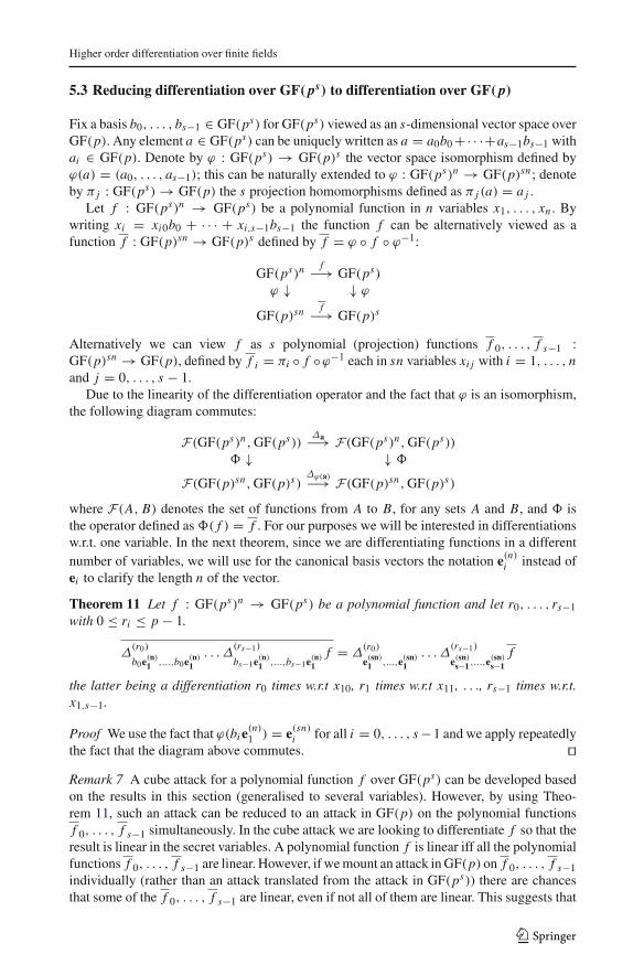
Fix a basis b0, . . . , bs−1 ∈ GF(ps) for GF(ps) viewed as an s-dimensional vector space overGF(p). Any element a ∈ GF(ps) can be uniquely written as a = a0b0+· · ·+as−1bs−1 withai ∈ GF(p). Denote by ϕ : GF(ps) → GF(p)s the vector space isomorphism defined byϕ(a) = (a0, . . . , as−1); this can be naturally extended to ϕ : GF(ps)n → GF(p)sn ; denoteby π j : GF(ps) → GF(p) the s projection homomorphisms defined as π j (a) = a j .
Let f : GF(ps)n → GF(ps) be a polynomial function in n variables x1, . . . , xn . Bywriting xi = xi0b0 + · · · + xi,s−1bs−1 the function f can be alternatively viewed as afunction f : GF(p)sn → GF(p)s defined by f = ϕ ◦ f ◦ ϕ−1:
GF(ps)nf−→ GF(ps)
ϕ ↓ ↓ ϕ
GF(p)snf−→ GF(p)s
Alternatively we can view f as s polynomial (projection) functions f 0, . . . , f s−1 :GF(p)sn → GF(p), defined by f i = πi ◦ f ◦ϕ−1 each in sn variables xi j with i = 1, . . . , nand j = 0, . . . , s − 1.
Due to the linearity of the differentiation operator and the fact that ϕ is an isomorphism,the following diagram commutes:
F(GF(ps)n,GF(ps))Δa−→ F(GF(ps)n,GF(ps))
� ↓ ↓ �
F(GF(p)sn,GF(p)s)Δϕ(a)−→ F(GF(p)sn,GF(p)s)
where F(A, B) denotes the set of functions from A to B, for any sets A and B, and � isthe operator defined as �( f ) = f . For our purposes we will be interested in differentiationsw.r.t. one variable. In the next theorem, since we are differentiating functions in a differentnumber of variables, we will use for the canonical basis vectors the notation e(n)
i instead ofei to clarify the length n of the vector.
Theorem 11 Let f : GF(ps)n → GF(ps) be a polynomial function and let r0, . . . , rs−1
with 0 ≤ ri ≤ p − 1.
Δ(r0)
b0e(n)1 ,...,b0e
(n)1
. . . Δ(rs−1)
bs−1e(n)1 ,...,bs−1e
(n)1
f = Δ(r0)
e(sn)1 ,...,e(sn)
1
. . . Δ(rs−1)
e(sn)s−1 ,...,e
(sn)s−1
f
the latter being a differentiation r0 times w.r.t x10, r1 times w.r.t x11, . . ., rs−1 times w.r.t.x1,s−1.
Proof We use the fact that ϕ(bie(n)1 ) = e(sn)
i for all i = 0, . . . , s−1 and we apply repeatedlythe fact that the diagram above commutes. �Remark 7 A cube attack for a polynomial function f over GF(ps) can be developed basedon the results in this section (generalised to several variables). However, by using Theo-rem 11, such an attack can be reduced to an attack in GF(p) on the polynomial functionsf 0, . . . , f s−1 simultaneously. In the cube attack we are looking to differentiate f so that theresult is linear in the secret variables. A polynomial function f is linear iff all the polynomialfunctions f 0, . . . , f s−1 are linear. However, if wemount an attack inGF(p) on f 0, . . . , f s−1individually (rather than an attack translated from the attack in GF(ps)) there are chancesthat some of the f 0, . . . , f s−1 are linear, even if not all of them are linear. This suggests that
123
A. Salagean et al.
for functions f over GF(ps) an attack in GF(p) on each component independently is morepromising than an attack in GF(ps) on the whole function f . Therefore, in Sect. 4.4 we onlydescribed the attack over GF(p).
6 Conclusion
We examined higher order differentiation over integers modulo a prime p, as well as overgeneral finite fields of ps elements, proving a number of results applicable to cryptographicattacks, and in particular generalising the fundamental theorem on which the cube attack isbased.
Using these results we proposed a generalisation of the cube attack to functions over theintegers modulo p; the main difference from the binary case is that we can differentiateseveral times with respect to the same variable. Such an attack would be particularly suitedto ciphers that use operations modulo p in their internal structure.
We also show that a further generalisation to general finite fields GF(ps) is possible, butnot as promising as the generalisation to GF(p), due to the fact that differentiation in GF(ps)can be reduced to differentiation in GF(p).
Acknowledgments Wewould like to thank Dr Iain Phillips and Haochen Zhu for their help in the implemen-tations discussed in Sect. 4.4.
Open Access This article is distributed under the terms of the Creative Commons Attribution 4.0 Interna-tional License (http://creativecommons.org/licenses/by/4.0/), which permits unrestricted use, distribution, andreproduction in any medium, provided you give appropriate credit to the original author(s) and the source,provide a link to the Creative Commons license, and indicate if changes were made.
References
1. Agnesse A., Pedicini M.: Cube attack in finite fields of higher order. In: Proceedings of the Ninth Aus-tralasian Information Security Conference—AISC ’11, vol. 116, pp. 9–14 (2011).
2. Aumasson J.-P., Dinur I., Meier W., Shamir A.: Cube testers and key recovery attacks on reduced-roundMD6 and Trivium. In: 16th International Workshop on Fast Software Encryption—FSE, pp. 1–22 (2009).
3. Biham E., Shamir A.: Differential cryptanalysis of DES-like cryptosystems. J. Cryptol. 4(1), 3–72 (1991).4. Daemen J., Govaerts R., Vandewalle J.: Block ciphers based on modular arithmetic. In: Wolfowicz W.
(ed.) Proceedings of the 3rd Symposium on the State and Progress of Research in Cryptography, pp.80–89. Fondazione Ugo Bordoni (1993).
5. Dinur I., Shamir A.: Cube attacks on tweakable black box polynomials. In: EUROCRYPT, pp. 278–299(2009).
6. Dodd F., Peele R.: Some counting problems involving the multinomial expansion. Math. Mag. 64(2),115–122 (1991).
7. Duan M., Lai X.: Higher order differential cryptanalysis framework and its applications. In: InternationalConference on Information Science and Technology (ICIST), pp. 291–297 (2011).
8. Ekdahl P., Johansson T.: SNOW—a new stream cipher. In: Proceedings of the First NESSIE Workshop.Heverlee, Belgium (2000).
9. ETSI/SAGE: Specification of the 3GPP confidentiality and integrity algorithms 128-EEA3 & 128-EIA3.Document 2: ZUC specification. Technical Report 1.6, ETSI, (2011).
10. Filiol E.: A new statistical testing for symmetric ciphers and hash functions. In: Deng R., Bao F., ZhouJ., Qing S. (eds.) Information and Communications Security. Lecture Notes in Computer Science, vol.2513, pp. 342–353. Springer, Berlin (2002).
11. Fouque P.-A., Vannet T.: Improving key recovery to 784 and 799 rounds of Trivium using optimized cubeattacks. In: 20th International Workshop on Fast Software Encryption—FSE, pp. 502–517 (2013).
12. Joux A.: Algorithmic Cryptanalysis, 1st edn. Chapman & Hall/CRC, Boca Raton (2009).
123
Higher order differentiation over finite fields
13. Kaufman T., Ron D.: Testing polynomials over general fields. In: Proceedings of the 45th Annual IEEESymposium on Foundations of Computer Science, pp. 413–422 (2004).
14. Knellwolf S., Meier W.: High order differential attacks on stream ciphers. Cryptogr. Commun. 4(3–4),203–215 (2012).
15. Kummer E.E.: Über die Ergänzungssätze zu den allgemeinen Reciprocitätsgesetzen J. Reine Angew.Math. 44, 93–146 (1852).
16. Lai X.: Higher order derivatives and differential cryptanalysis. In: Blahut R.E., Costello D.J., Jr., Mau-rer U., Mittelholzer T. (eds.) Communications and Cryptography. The Springer International Series inEngineering and Computer Science, vol. 276, pp. 227–233. Springer, Berlin (1994).
17. Lai X., Massey J.L.: A proposal for a new block encryption standard. In: EUROCRYPT, pp. 389–404(1990).
18. Lai X., Massey J.L., Murphy S.: Markov ciphers and differential cryptanalysis. In: EUROCRYPT, pp.17–38 (1991).
19. MacWilliams F.J., Sloane N.J.A.: The Theory of Error-Correcting Codes. North Holland, Amsterdam(1977).
20. O’Neil S.: Algebraic structure defectoscopy. Cryptology ePrint Archive, Report 2007/378. http://eprint.iacr.org/ (2007).
21. Vielhaber M.: Breaking ONE.FIVIUM by AIDA an algebraic IV differential attack. Cryptology ePrintArchive, Report 2007/413. http://eprint.iacr.org/ (2007).
22. VielhaberM.: AIDAbreaks BIVIUM (A&B) in 1minute dual core CPU time. Cryptology ePrint Archive,Report 2009/402. http://eprint.iacr.org/ (2009).
23. Winter R., Salagean A., Phan R.C.W.: Comparison of cube attacks over different vector spaces. In: Groth,J. (ed.) 15th IMA International Conference on Cryptography and Coding, IMACC. Lecture Notes inComputer Science, vol. 9496, pp. 225–238. Springer, Berlin (2015).
123