© Lakshmi Sankar 2002 1
Steady, Level Forward Flight
I . Introductory Remarks
© Lakshmi Sankar 2002 2
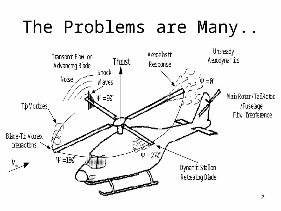
The Problems are Many..
ThrustAeroelasticResponse
0
270 180
90
Dynamic Stall onRetreating Blade
Blade-Tip Vortexinteractions
UnsteadyAerodynamicsTransonic Flow on
Advancing Blade
Main Rotor / Tail Rotor/ Fuselage
Flow Interference
V
NoiseShock Waves
Tip Vortices
© Lakshmi Sankar 2002 3
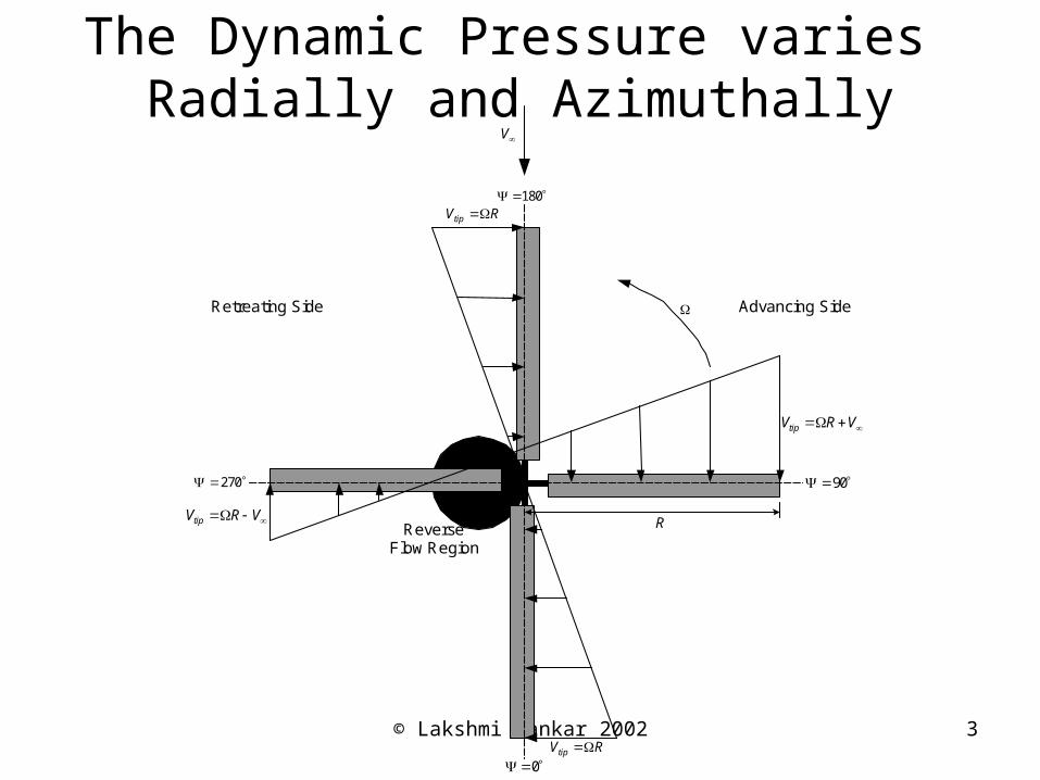
The Dynamic Pressure varies Radially and Azimuthally
0
270
180
90
V
RVtip
RVtip
VRVtip
VRVtip
RReverseFlow Region
Advancing SideRetreating Side
© Lakshmi Sankar 2002 4
Consequences of Forward Flight
• The dynamic pressure, and hence the air loads have high harmonic content. Above some speed, vibrations can limit safe operations.
• On the advancing side, high dynamic pressure will cause shock waves, and too high a lift (unbalanced). – To counter this, the blade may need to flap up (or pitch down) to
reduce the angle of attack.• Low dynamic pressure on the retreating side.• The blade may need to flap down or pitch up to increase
angle of attack on the retreating side. This can cause dynamic stall.
• Total lift decreases as the forward speed increases as a consequence of these effects, setting a upper limit on forward speed.
© Lakshmi Sankar 2002 5
Forward Flight Analysis thus requires
• Performance Analysis – How much power is needed?
• Blade Dynamics and Control – What is the flapping dynamics? How does the pilot input alters the blade behavior? Is the rotor and the vehicle trimmed?
• Airload prediction over the entire rotor disk using blade element theory, which feeds into vibration analysis, aeroelastic studies, and acoustic analyses.
• We will look at some of these elements.
© Lakshmi Sankar 2002 6
Steady, Level Forward Flight
II. Performance
© Lakshmi Sankar 2002 7
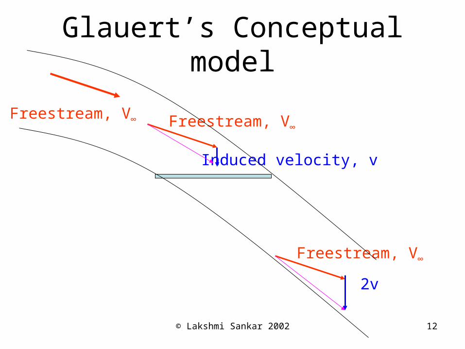
Inflow Model
• To start this effort, we will need a very simple inflow model.
• A model proposed by Glauert is used.• This model is phenomenological, not
mathematically well founded.• It gives reasonable estimates of inflow velocity at
the rotor disk, and is a good starting point.• It also gives the correct results for an elliptically
loaded wing.
© Lakshmi Sankar 2002 8
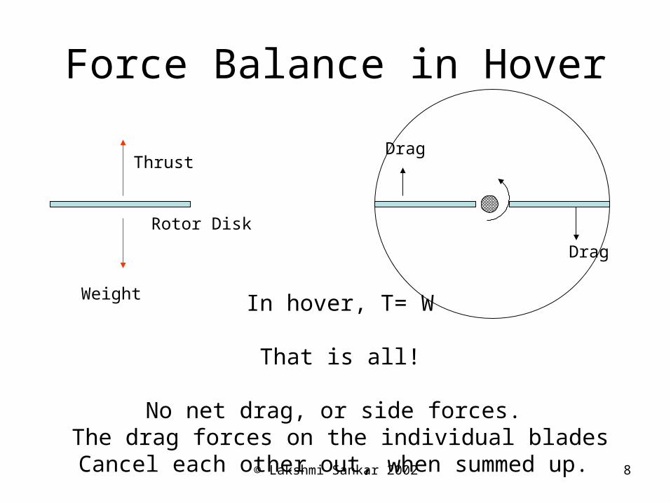
Force Balance in Hover
Thrust
Weight In hover, T= W
That is all!
No net drag, or side forces. The drag forces on the individual blades
Cancel each other out, when summed up.
Drag
Drag
Rotor Disk
© Lakshmi Sankar 2002 9
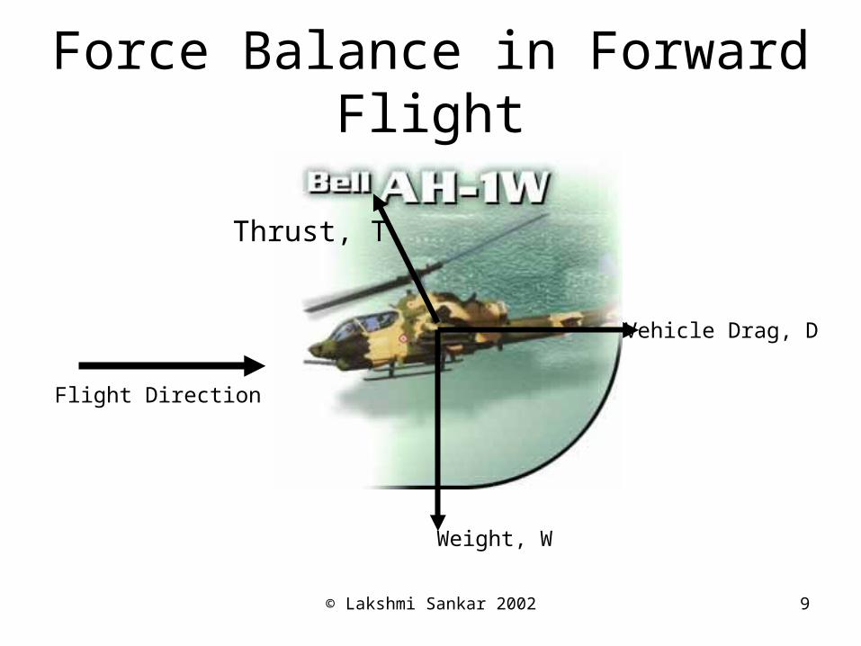
Force Balance in Forward Flight
Flight Direction
Weight, W
Vehicle Drag, D
Thrust, T
© Lakshmi Sankar 2002 10
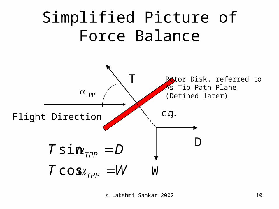
Simplified Picture of Force Balance
T
W
D
c.g. Flight Direction
TPP
Rotor Disk, referred toAs Tip Path Plane(Defined later)
WT
DT
TPP
TPP
cos
sin
© Lakshmi Sankar 2002 11
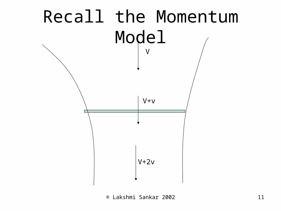
Recall the Momentum ModelV
V+v
V+2v
© Lakshmi Sankar 2002 12
Glauert’s Conceptual model
Freestream, V∞ Freestream, V∞
Induced velocity, v
Freestream, V∞
2v
© Lakshmi Sankar 2002 13
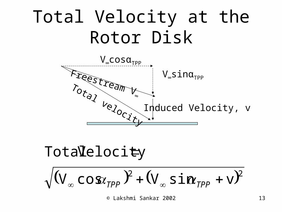
Total Velocity at the Rotor Disk
Freestream V∞
Induced Velocity, v
V∞cosαTPP
V∞sinαTPP
Total velocity
22 vsinVcosV
Velocity Total
TPPTPP
© Lakshmi Sankar 2002 14
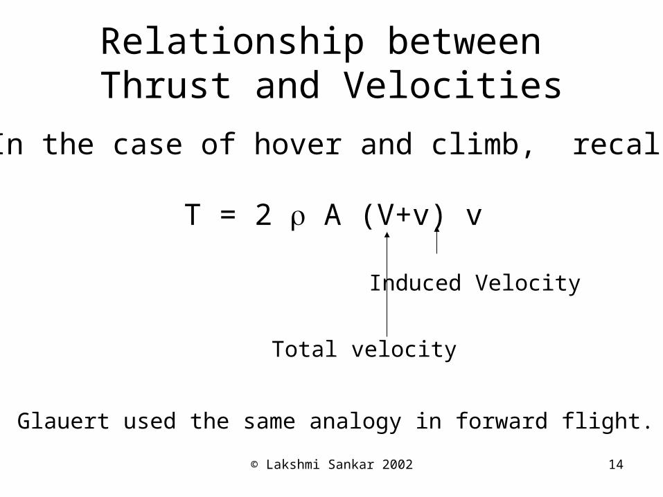
Relationship between Thrust and Velocities
In the case of hover and climb, recall
T = 2 A (V+v) v
Induced Velocity
Total velocity
Glauert used the same analogy in forward flight.
© Lakshmi Sankar 2002 15
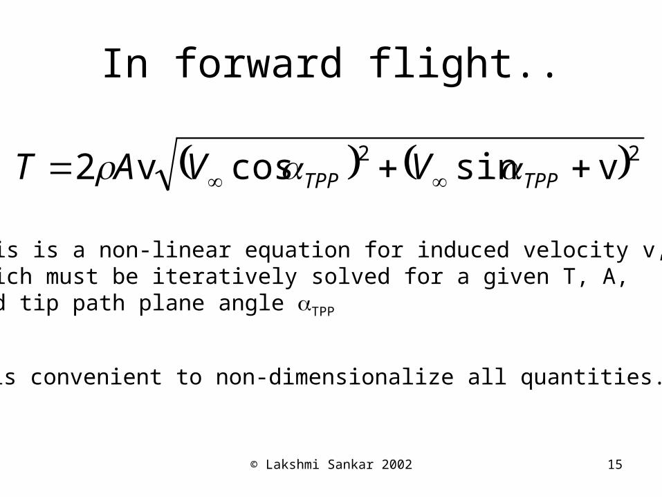
In forward flight..
22 vsincosv2 TPPTPP VVAT
This is a non-linear equation for induced velocity v, which must be iteratively solved for a given T, A, and tip path plane angle TPP
It is convenient to non-dimensionalize all quantities.
© Lakshmi Sankar 2002 16
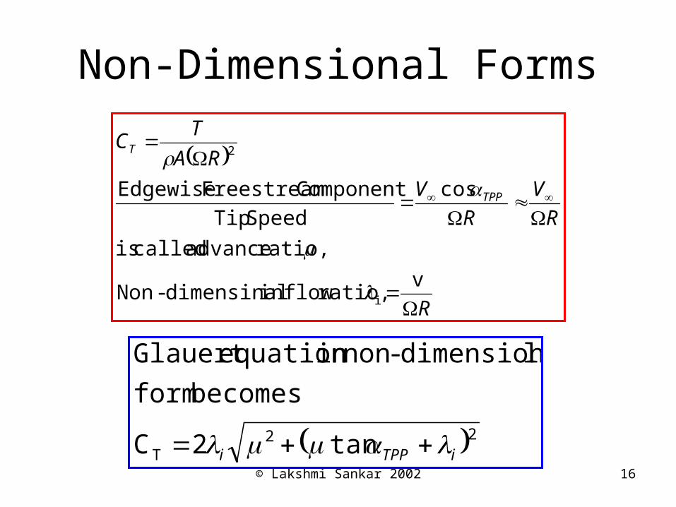
Non-Dimensional Forms
R
R
V
R
V
RA
TC
TPP
T
v ratio, inflow dimensinal-Non
ratio, advance called is
cos
Speed Tip
Component Freestream Edgewise
i
2
22T tan2C
becomes form
ldimensiona-nonin equation Glauert
iTPPi
© Lakshmi Sankar 2002 17
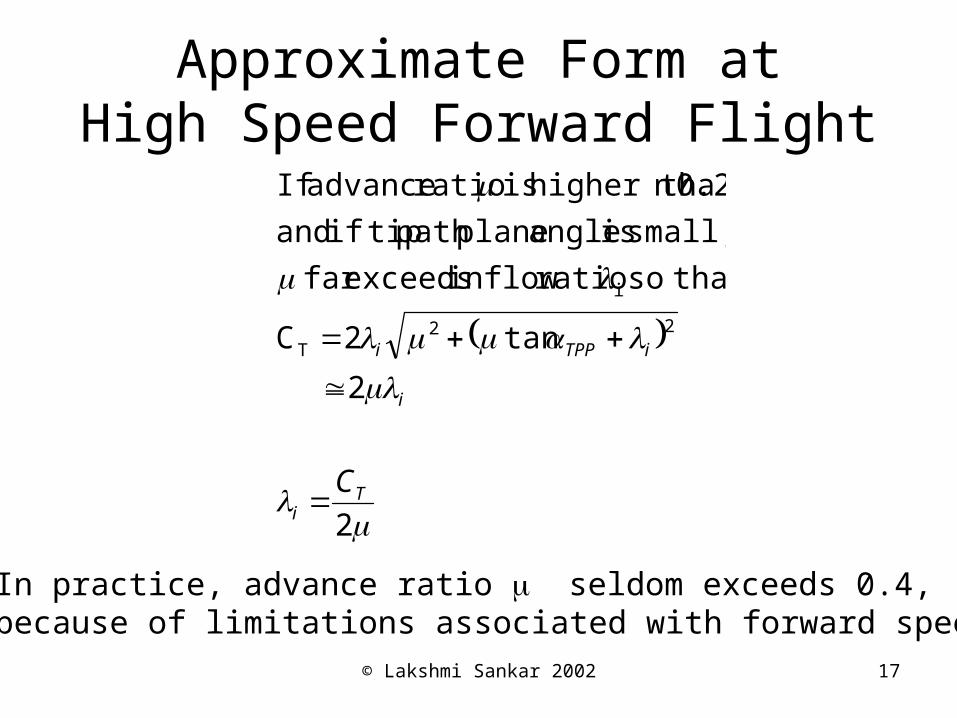
Approximate Form atHigh Speed Forward Flight
2
2
tan2C
thatso ratio inflow exceedsfar
small, is angle planepath tipif and
0.2,n higher tha is ratio advance If
22T
i
Ti
i
iTPPi
C
In practice, advance ratio seldom exceeds 0.4, because of limitations associated with forward speed.
© Lakshmi Sankar 2002 18
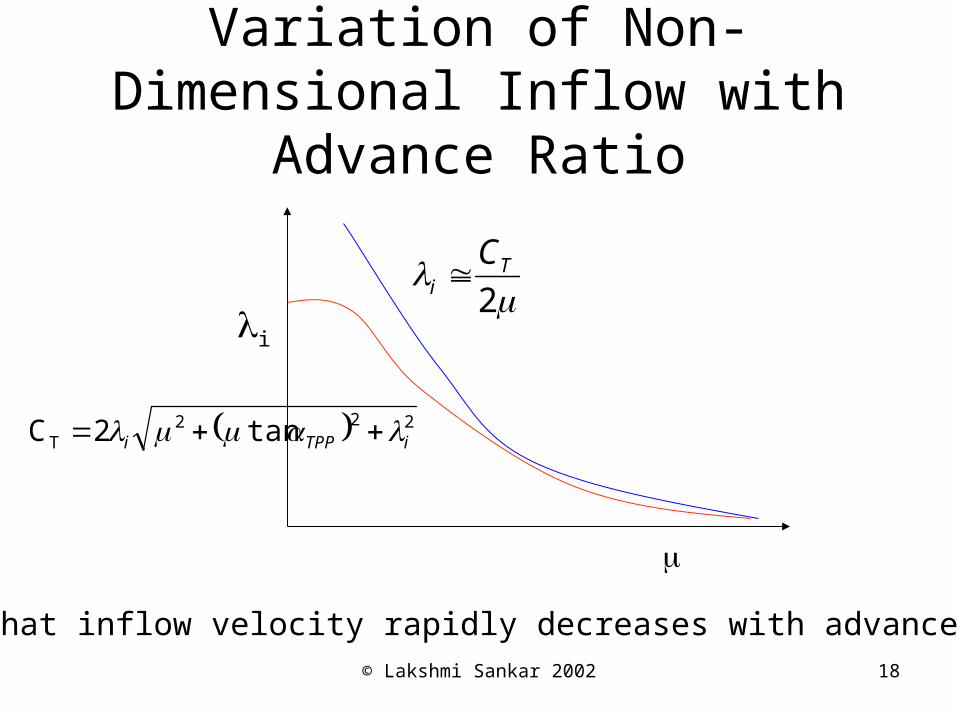
Variation of Non-Dimensional Inflow with Advance Ratio
222T tan2C iTPPi
i
2T
i
C
Notice that inflow velocity rapidly decreases with advance ratio.
© Lakshmi Sankar 2002 19
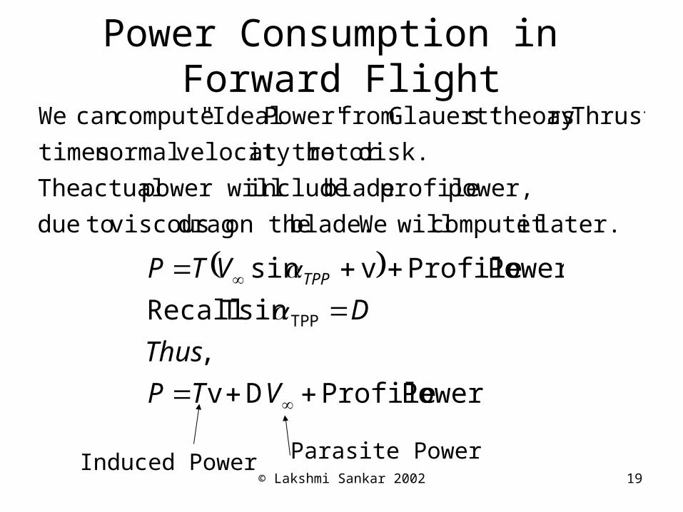
Power Consumption in Forward Flight
later.it compute will Weblade. on the drag viscous todue
power, profile blade include power will actual The
disk.rotor at the velocity normal times
Thrust as theory sGlauert' from Power" Ideal" computecan We
Power ProfileDv
,
Tsin Recall
Power Profilevsin
TPP
VTP
Thus
D
VTP TPP
Induced Power Parasite Power
© Lakshmi Sankar 2002 20
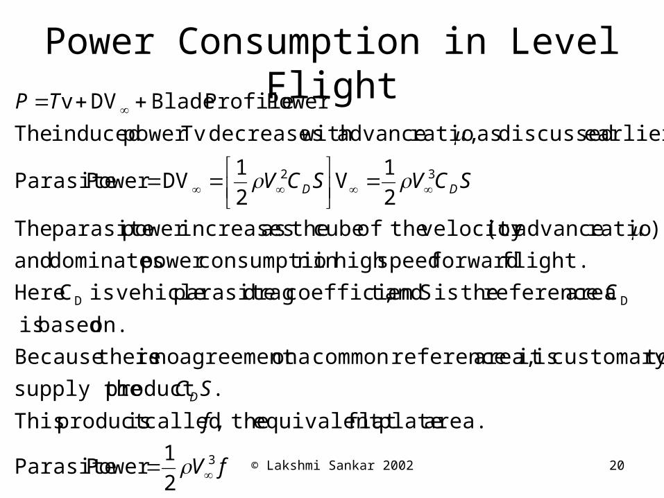
Power Consumption in Level Flight
fV
f
SC
SCVSCV
TP
D
DD
3
DD
32
2
1Power Parasite
area. plateflat equivalent the, called isproduct This
.product supply the
tocustomary isit area, referencecommon aon agreement no is thereBecause
on. based is
C area reference theis S and t,coefficien drag parasite vehicleis C Here
flight. forward speedhigh in n consumptiopower dominates and
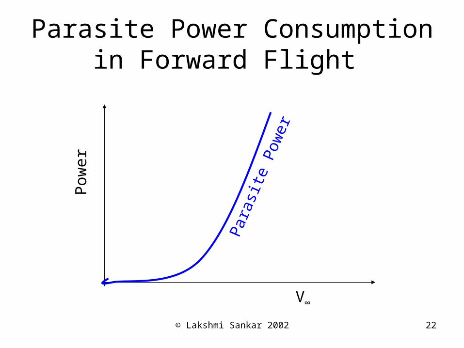
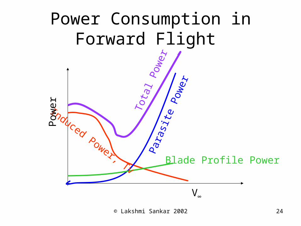
) ratio advance(or velocity theof cube theas increasespower parasite The
2
1V
2
1DVPower Parasite
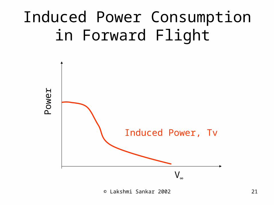
earlier. discussed as , ratio advance with decreases Tvpower induced The
Power Profile Blade DVv
© Lakshmi Sankar 2002 21
Induced Power Consumption in Forward Flight
Induced Power, Tv
V∞
Pow
er
© Lakshmi Sankar 2002 22
Parasite Power Consumption in Forward Flight
Par
asite
Pow
erV∞
Pow
er
© Lakshmi Sankar 2002 23
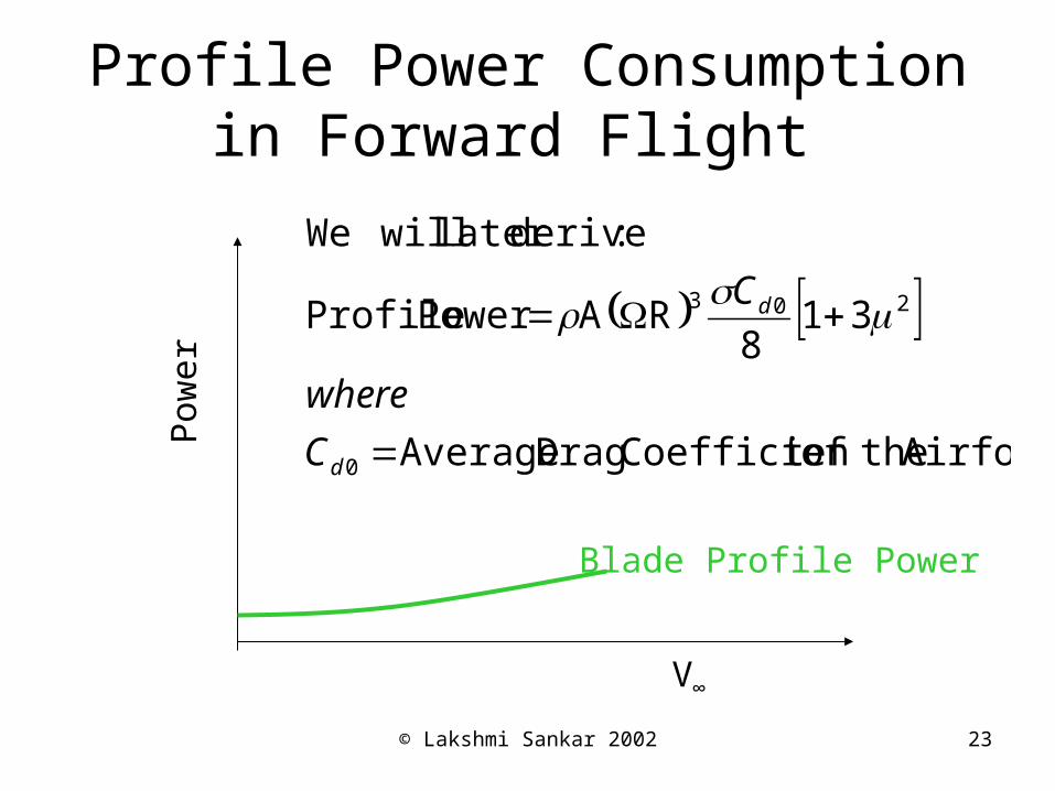
Profile Power Consumption in Forward Flight
Blade Profile Power
V∞
Pow
er
Airfoil theoft Coefficien Drag Average
318
RAPower Profile
:derivelater willWe
0
203
d
d
C
where
C
© Lakshmi Sankar 2002 24
Power Consumption in Forward Flight
Induced Power, TvP
aras
ite P
ower
Blade Profile Power
V∞
Pow
er Tota
l Pow
er
© Lakshmi Sankar 2002 25
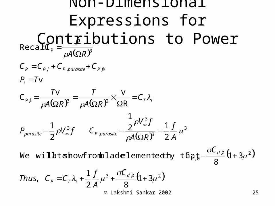
Non-Dimensional Expressions for Contributions to Power
20,3
20,P,0
33
3
,3
23iP,
0,,,
3P
3182
1 ,
318
Ceory that element th blade from showlater willWe
2
121
2
1
R
vvC
v
C :Recall
diTP
d
parasitePparasite
iT
i
PparasitePiPP
C
A
fCCThus
C
A
f
RA
fVCfVP
CRA
T
RA
T
TP
CCCC
RA
P
© Lakshmi Sankar 2002 26
Empirical Corrections
• The performance theory above does not account for– Non-uniform inflow effects– Swirl losses– Tip Losses
• It also uses an average drag coefficient.
• To account for these, the power coefficient is empirically corrected.
© Lakshmi Sankar 2002 27
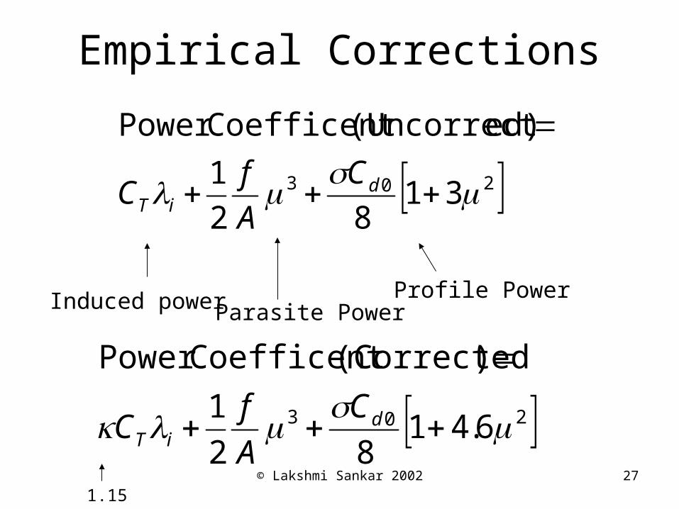
Empirical Corrections
203 3182
1
ed)(Uncorrect CoefficentPower
diT
C
A
fC
Induced power Parasite PowerProfile Power
203 6.4182
1
)(Corrected CoefficentPower
diT
C
A
fC
1.15
© Lakshmi Sankar 2002 28
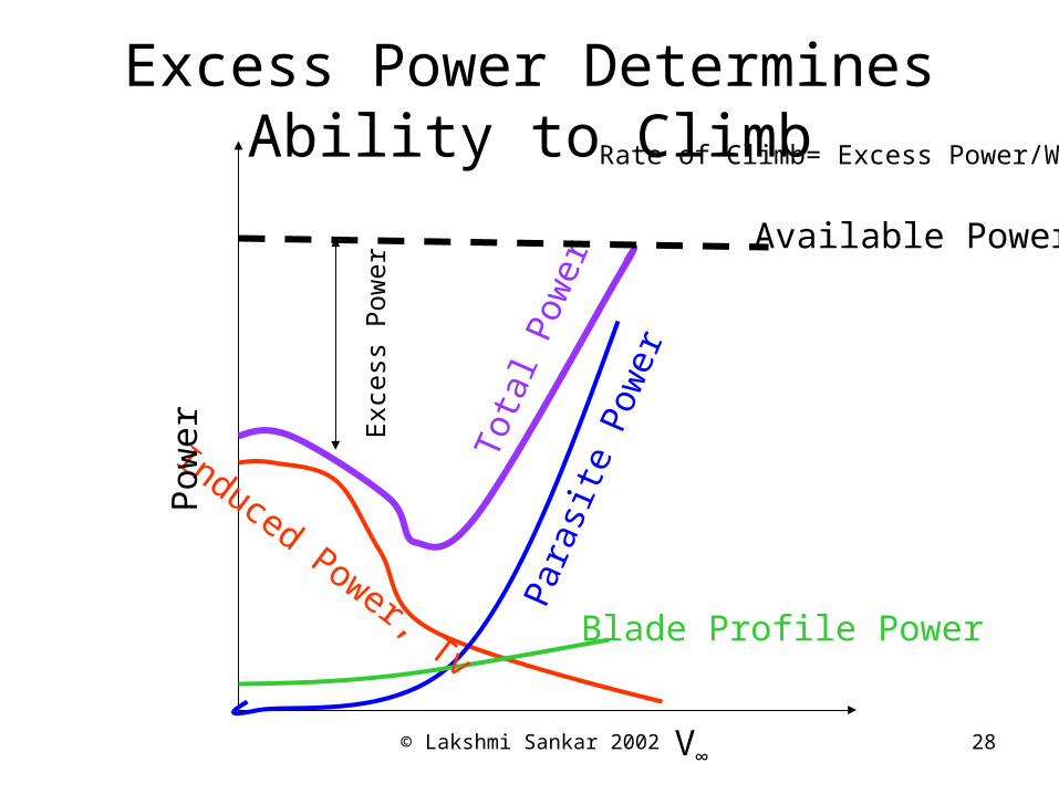
Excess Power Determines Ability to Climb
Induced Power, Tv
Par
asite
Pow
erBlade Profile Power
V∞
Pow
er Tota
l Pow
er
Available Power
Exc
ess
Pow
er
Rate of Climb= Excess Power/W
© Lakshmi Sankar 2002 29
Forward Flight
Blade Dynamics
© Lakshmi Sankar 2002 30
Background
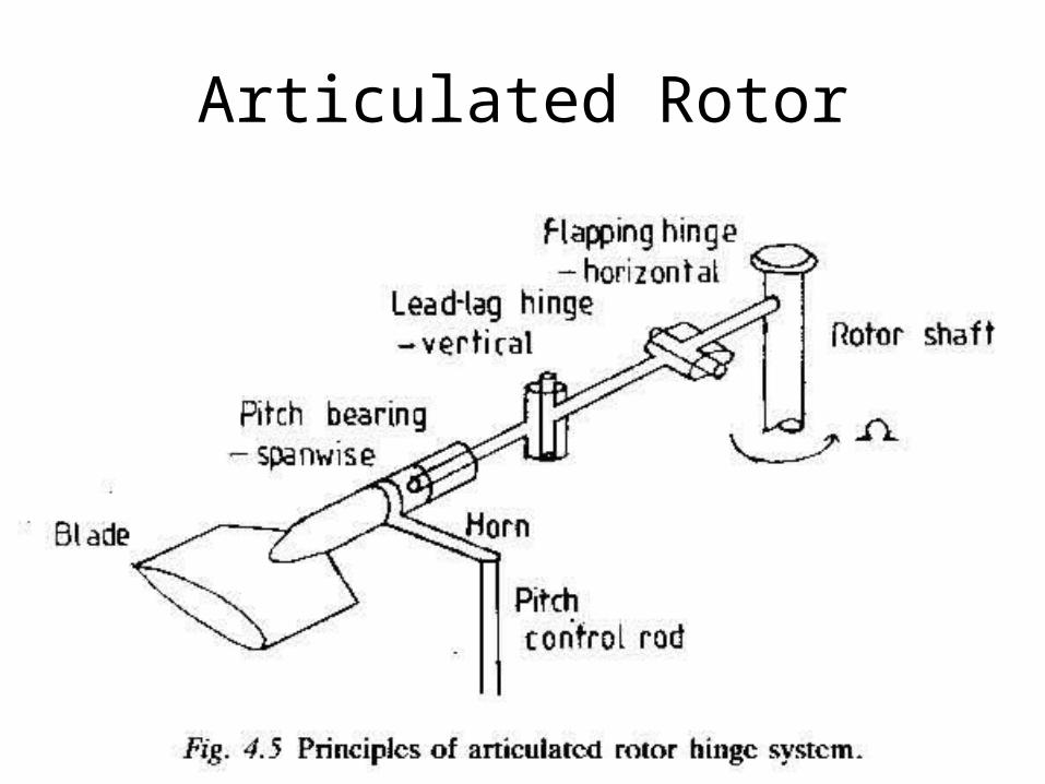
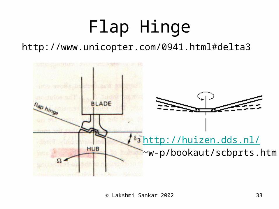
• Helicopter blades are attached to the rotor shaft with a series of hinges:– Flapping hinges (or a soft flex-beam) , that allow blades to freely
flap up or down. This ensures that lift is transferred to the shaft, but not the moments.
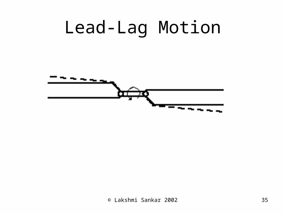
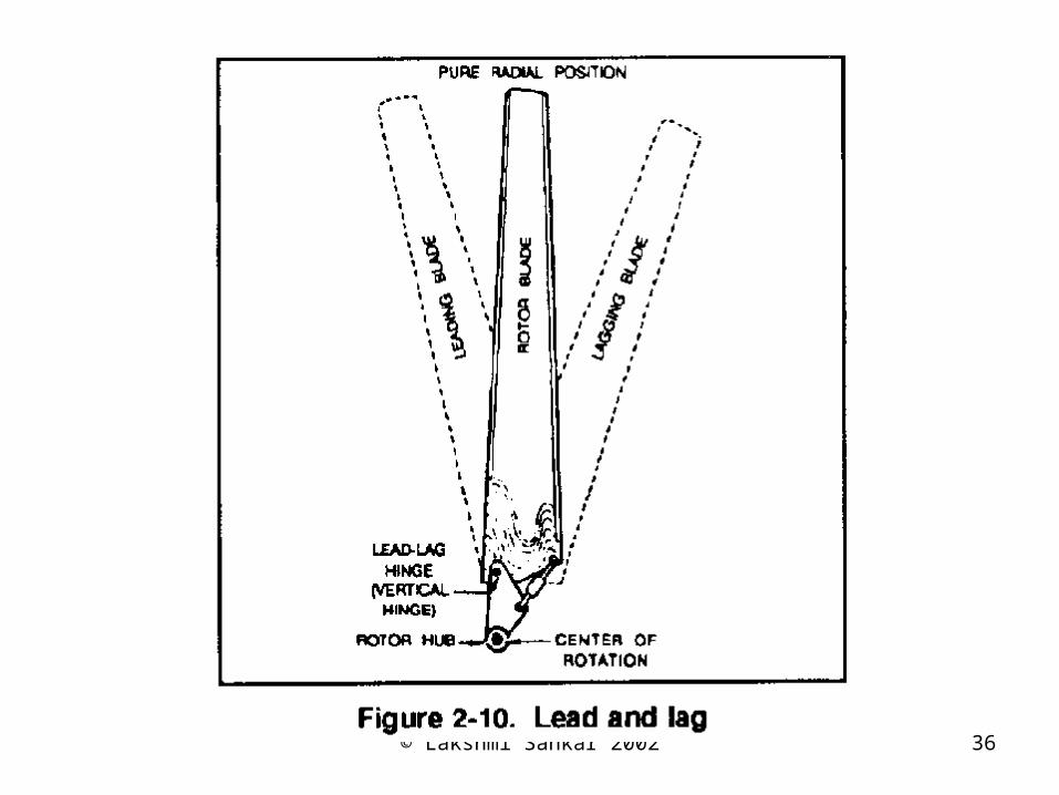
– Lead-Lag Hinges. When the blades rotate, and flap, Coriolis forces are created in the plane of the rotor. In order to avoid unwanted stresses at the blade root, lead-lag hinges are used.
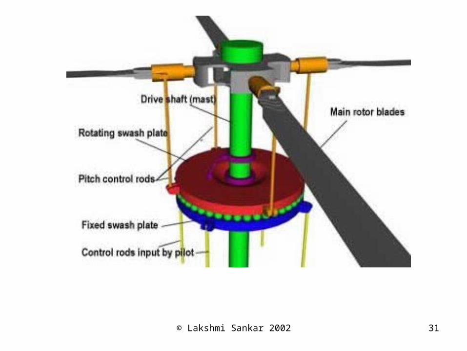
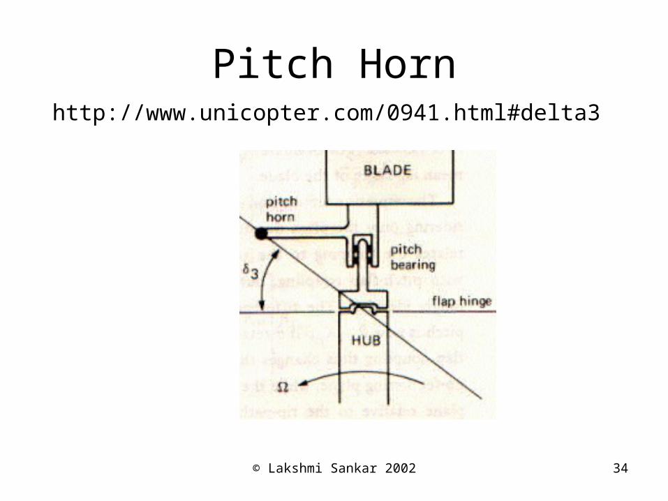
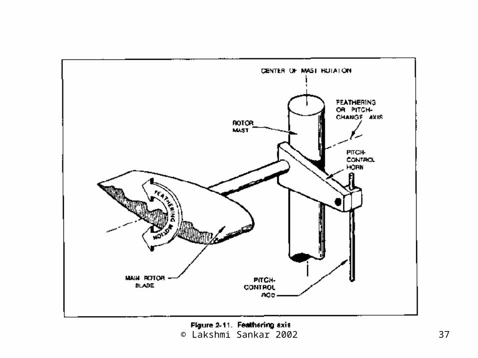
– Pitch bearing/pitch-link/swash plate: Used to control the blade pitch.
• The blade loads are affected by the motion of the blades about these hinges.
• From an aerodynamic perspective, lead-lag motion can be neglected. Pitching and flapping motions must be included.
© Lakshmi Sankar 2002 31
© Lakshmi Sankar 2002 32
Articulated Rotor
© Lakshmi Sankar 2002 33
Flap Hingehttp://www.unicopter.com/0941.html#delta3
http://huizen.dds.nl/~w-p/bookaut/scbprts.htm
© Lakshmi Sankar 2002 34
Pitch Hornhttp://www.unicopter.com/0941.html#delta3
© Lakshmi Sankar 2002 36
© Lakshmi Sankar 2002 37
© Lakshmi Sankar 2002 38
Coordinate Systems
• Before we start defining the blade motion, and the blade angular positions, it is necessary to define what is the coordinate system to use.
• Unfortunately, there are many possible coordinate systems. No unique choice.
© Lakshmi Sankar 2002 39
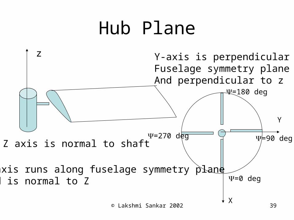
Hub Planez
X
Y
Z axis is normal to shaft
X-axis runs along fuselage symmetry planeAnd is normal to Z
Y-axis is perpendicular toFuselage symmetry planeAnd perpendicular to z
=0 deg
=90 deg
=180 deg
=270 deg
© Lakshmi Sankar 2002 40
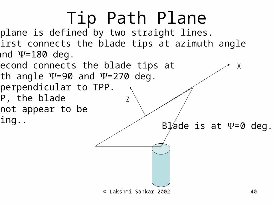
This plane is defined by two straight lines.The first connects the blade tips at azimuth angle =0 and =180 deg.The second connects the blade tips at azimuth angle =90 and =270 deg.Z is perpendicular to TPP.In TPP, the bladeDoes not appear to beFlapping..
Tip Path Plane
X
Z
Blade is at =0 deg.
© Lakshmi Sankar 2002 41
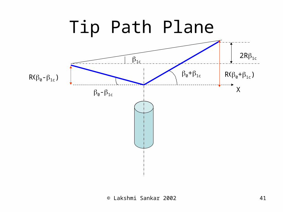
Tip Path Plane
X
0+1c
0-1c
R0+1c)R0-1c)
2R1c1c
© Lakshmi Sankar 2002 42
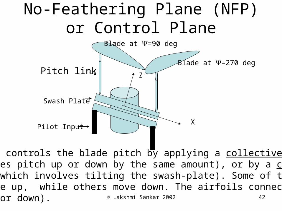
No-Feathering Plane (NFP) or Control Plane
The pilot controls the blade pitch by applying a collective control (all blades pitch up or down by the same amount), or by a cyclic control (which involves tilting the swash-plate). Some of the pitch links move up, while others move down. The airfoils connected pitch up or down).
X
ZPitch link
Swash Plate
Pilot Input
Blade at =90 deg
Blade at =270 deg
© Lakshmi Sankar 2002 43
Differences between Various Systems
• For an observer sitting on the tip path plane, the blade tips appear to be touching the plane all the time. There is no flapping motion in this coordinate system.
• For an observer sitting on the swash plate, the pitch links will appear to be stationary. There is no vertical up or down motion of the pitch links, and no pitching motion of the blades either.
• In the shaft plane, the blades will appear to pitch and flap, both.
• One can use any one of these coordinate systems for blade element theory. Some coordinate systems are easier to work with. For example, in the TPP we can set the flapping motion to zero.
© Lakshmi Sankar 2002 44
Forward Flight
Blade Flapping Dynamics and Response
© Lakshmi Sankar 2002 45
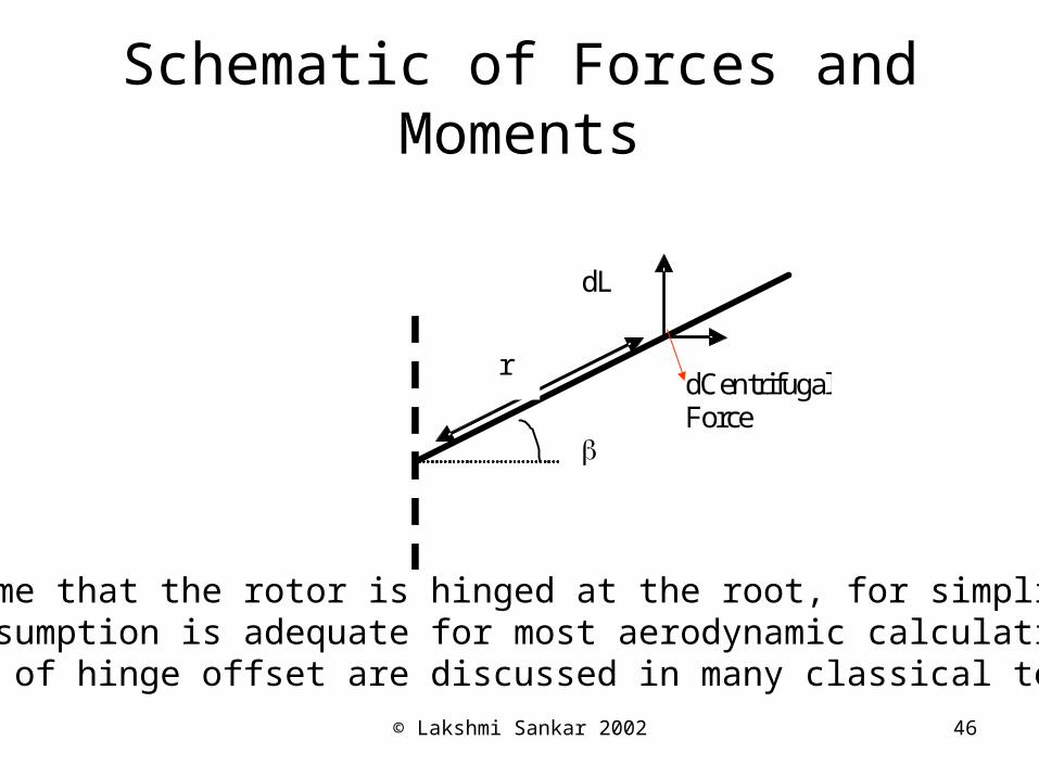
Background
• As seen earlier, blades are usually hinged near the root, to alleviate high bending moments at the root.
• This allows the blades to flap up and down.• Aerodynamic forces cause the blades to flap up.• Centrifugal forces causes the blades to flap down.• Inertial forces will arise, which oppose the direction of
acceleration.• In forward flight, an equilibrium position is achieved,
where the net moments at the hinge due to these three types of forces (aerodynamic, centrifugal, inertial) cancel out and go to zero.
© Lakshmi Sankar 2002 46
Schematic of Forces and Moments
dL
dCentrifugal Force
r
We assume that the rotor is hinged at the root, for simplicity.This assumption is adequate for most aerodynamic calculations.Effects of hinge offset are discussed in many classical texts.
© Lakshmi Sankar 2002 47
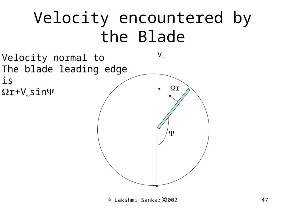
Velocity encountered by the Blade
V∞
X
r
Velocity normal toThe blade leading edgeisr+V∞sin
© Lakshmi Sankar 2002 48
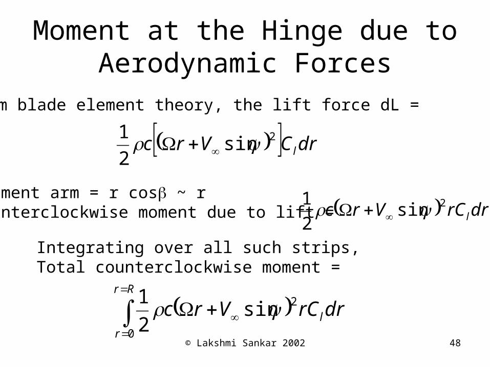
Moment at the Hinge due toAerodynamic Forces
From blade element theory, the lift force dL =
drCVrc l2sin
2
1
Moment arm = r cos ~ rCounterclockwise moment due to lift = drrCVrc l
2sin2
1
Integrating over all such strips,Total counterclockwise moment =
Rr
r
ldrrCVrc0
2sin2
1
© Lakshmi Sankar 2002 49
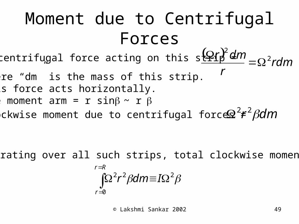
Moment due to Centrifugal Forces
The centrifugal force acting on this strip = rdm
r
dmr 22
Where “dm” is the mass of this strip.This force acts horizontally. The moment arm = r sin ~ rClockwise moment due to centrifugal forces = dmr 22
Integrating over all such strips, total clockwise moment =
2
0
22
IdmrRr
r
© Lakshmi Sankar 2002 50
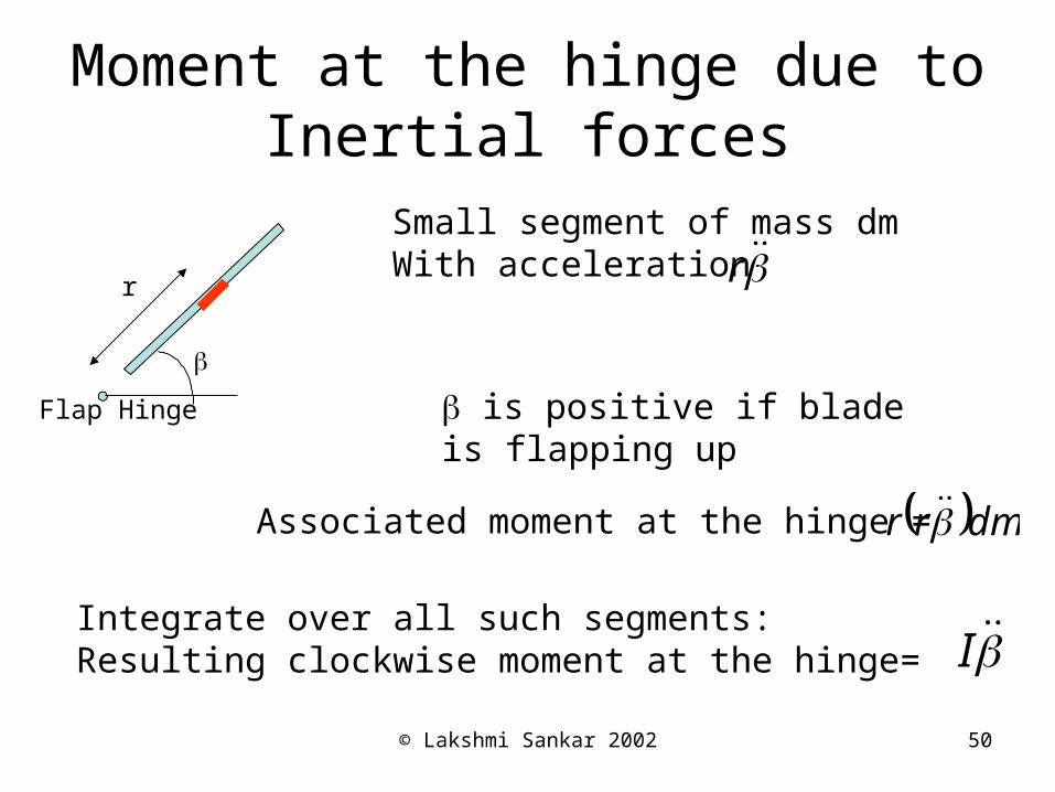
Moment at the hinge due to Inertial forces
r
dmrr
Small segment of mass dmWith acceleration
is positive if blade is flapping up
Associated moment at the hinge =
r
Flap Hinge
Integrate over all such segments: Resulting clockwise moment at the hinge= I
© Lakshmi Sankar 2002 51
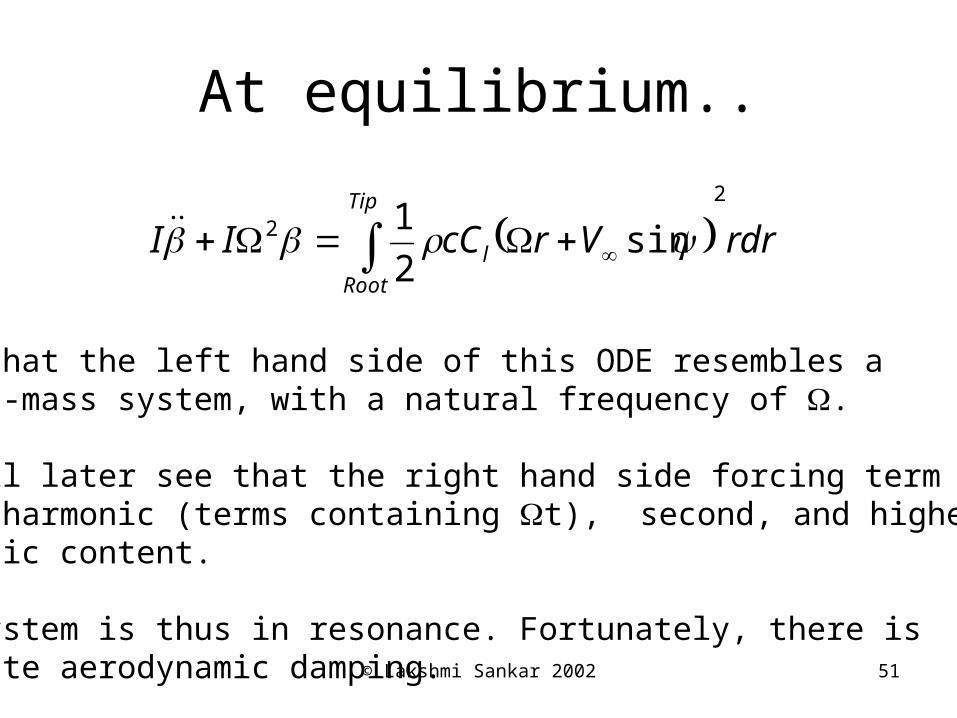
At equilibrium..
rdrVrcCIITip
Root
l
2
2 sin2
1
Note that the left hand side of this ODE resembles a spring-mass system, with a natural frequency of .
We will later see that the right hand side forcing term has first harmonic (terms containing t), second, and higher Harmonic content.
The system is thus in resonance. Fortunately, there isAdequate aerodynamic damping.
© Lakshmi Sankar 2002 52
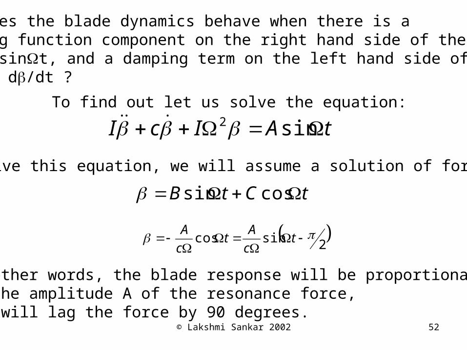
How does the blade dynamics behave when there is a forcing function component on the right hand side of the form Asint, and a damping term on the left hand side of form c d/dt ?
To find out let us solve the equation:
tAIcI sin2
To solve this equation, we will assume a solution of form:
tCtB cossin
2sincos
tc
At
c
A
In other words, the blade response will be proportional to the amplitude A of the resonance force, but will lag the force by 90 degrees.
© Lakshmi Sankar 2002 53
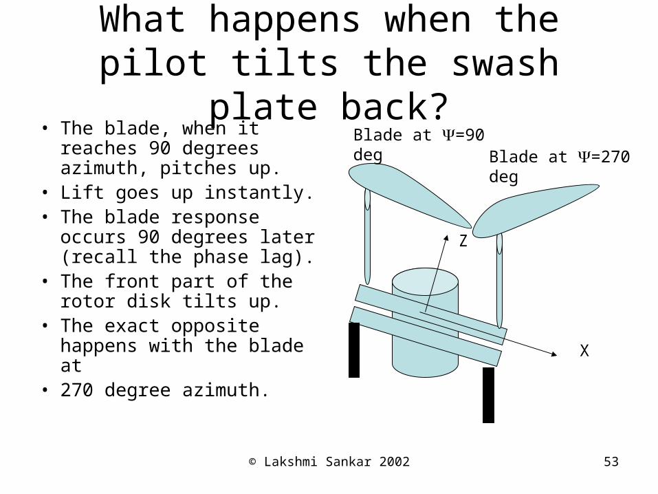
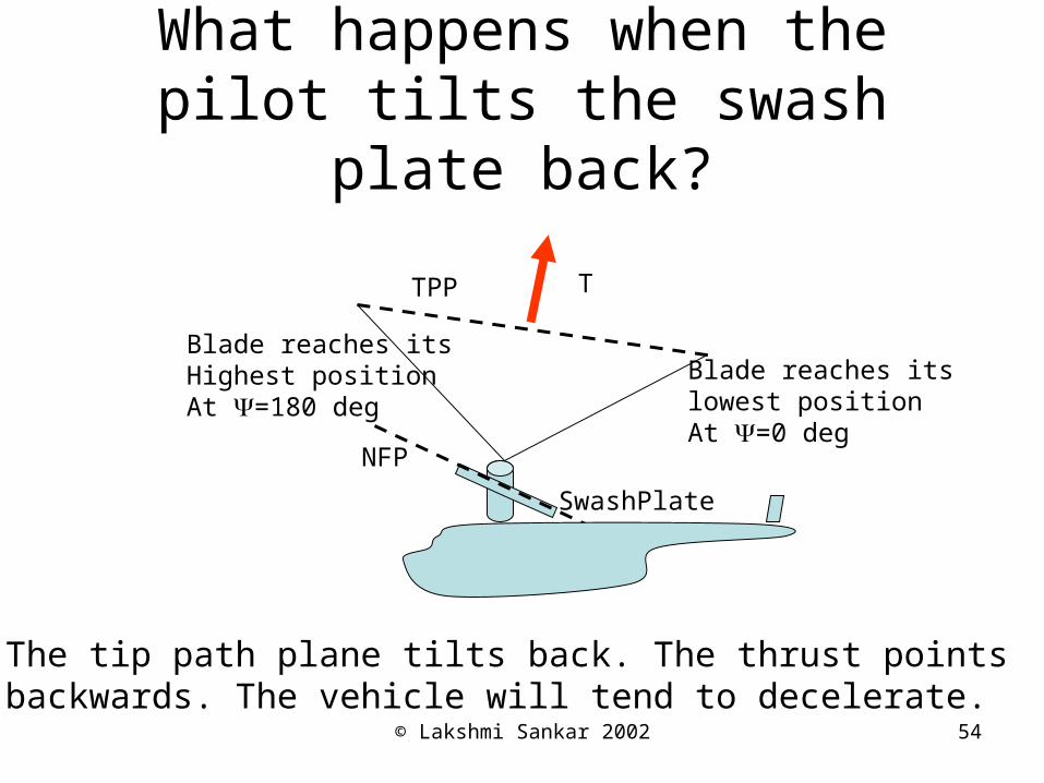
What happens when the pilot tilts the swash plate back?
• The blade, when it reaches 90 degrees azimuth, pitches up.
• Lift goes up instantly.• The blade response
occurs 90 degrees later (recall the phase lag).
• The front part of the rotor disk tilts up.
• The exact opposite happens with the blade at
• 270 degree azimuth.
X
Z
Blade at =270 deg
Blade at =90 deg
© Lakshmi Sankar 2002 54
What happens when the pilot tilts the swash plate back?
Blade reaches itsHighest positionAt =180 deg
Blade reaches itslowest positionAt =0 deg
T
SwashPlate
The tip path plane tilts back. The thrust points backwards. The vehicle will tend to decelerate.
TPP
NFP
© Lakshmi Sankar 2002 55
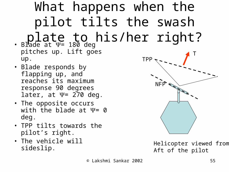
What happens when the pilot tilts the swash plate to his/her right?
• Blade at = 180 degpitches up. Lift goes up.
• Blade responds by flapping up, and reaches its maximum response 90 degrees later, at = 270 deg.
• The opposite occurs with the blade at = 0 deg.
• TPP tilts towards the pilot’s right.
• The vehicle will sideslip.
TPP
Helicopter viewed fromAft of the pilot
NFP
T
© Lakshmi Sankar 2002 56
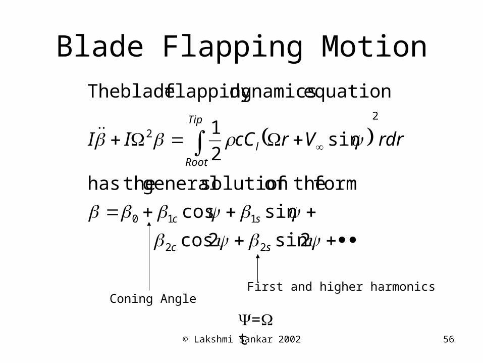
Blade Flapping Motion
2sin2cos
sincos
form theofsolution general thehas
sin2
1
equation dynamics flapping blade The
22
110
2
2
sc
sc
Tip
Root
l rdrVrcCII
Coning AngleFirst and higher harmonics
=t
© Lakshmi Sankar 2002 57
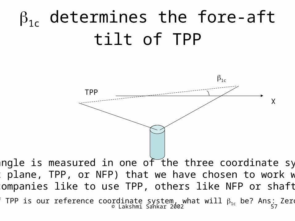
1c determines the fore-aft tilt of TPP
1c
X
This angle is measured in one of the three coordinate systems (Shaft plane, TPP, or NFP) that we have chosen to work with.Some companies like to use TPP, others like NFP or shaft plane.
TPP
If TPP is our reference coordinate system, what will 1c be? Ans: Zero.
© Lakshmi Sankar 2002 58
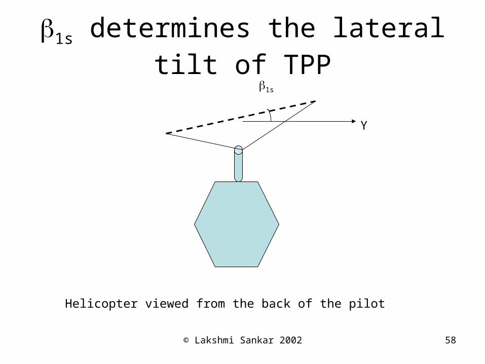
1s determines the lateral tilt of TPP
Y
1s
Helicopter viewed from the back of the pilot
© Lakshmi Sankar 2002 59
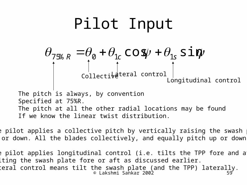
Pilot Input
sincos 110%75 scR
The pitch is always, by conventionSpecified at 75%R.The pitch at all the other radial locations may be foundIf we know the linear twist distribution.
Collective Lateral controlLongitudinal control
The pilot applies a collective pitch by vertically raising the swash plate up or down. All the blades collectively, and equally pitch up or down.
The pilot applies longitudinal control (i.e. tilts the TPP fore and aft) byTilting the swash plate fore or aft as discussed earlier. Lateral control means tilt the swash plate (and the TPP) laterally.
© Lakshmi Sankar 2002 60
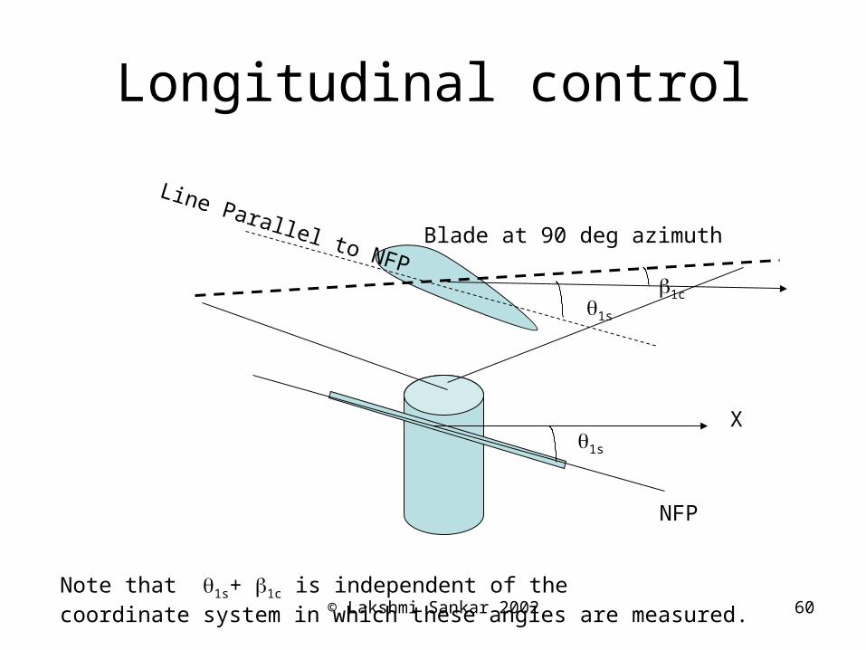
Longitudinal control
Blade at 90 deg azimuth
NFP
Line Parallel to NFP
X1s
1c
Note that 1s+ 1c is independent of the coordinate system in which these angles are measured.
1s
© Lakshmi Sankar 2002 61
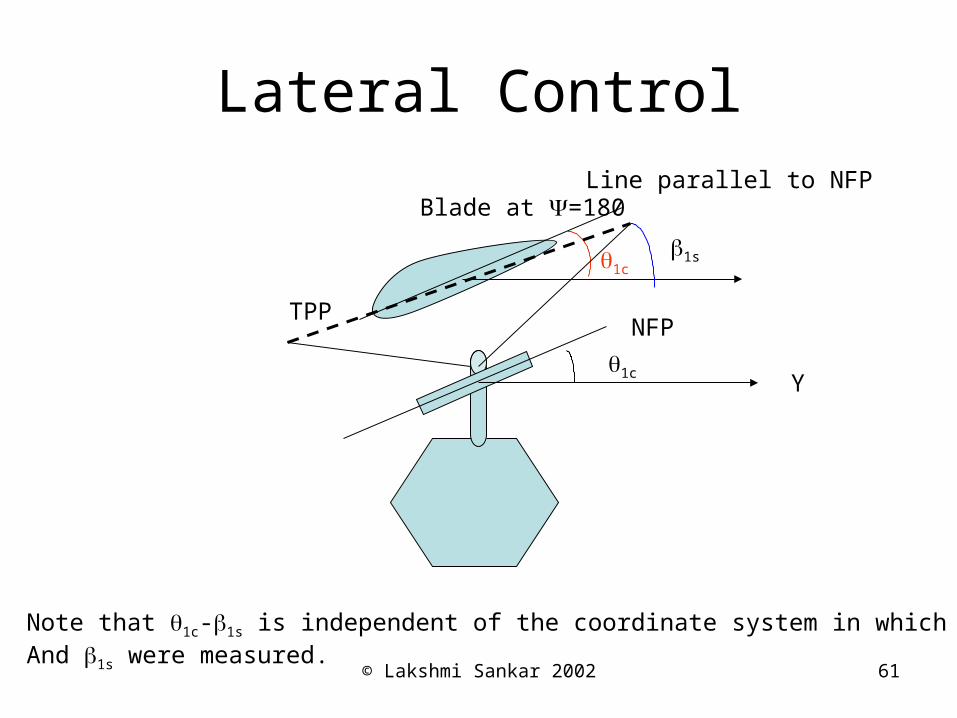
Lateral Control
Y1c
NFP
Line parallel to NFP
1c
Blade at =180
1s
Note that 1c-1s is independent of the coordinate system in which 1c
And 1s were measured.
TPP

© Lakshmi Sankar 2002 62
As a result..
TPPcNFPscs
TPPsNFPcsc
1111
1111
© Lakshmi Sankar 2002 63
In the future..
• We will always see 1c+1s appear in pair.• We will always see 1s-1c appear in pair.• As far as the blade sections are
concerned, to them it does not matter if the aerodynamic loads on them are caused by one degree of pitch that the pilot inputs in the form of 1c or 1s, or by one degree of flapping (1c or 1s).
• One degree of pitch= One degree of flap.
© Lakshmi Sankar 2002 64
Forward Flight
Angle of Attack of the Airfoil
And
Sectional Load Calculations
© Lakshmi Sankar 2002 65
The angle of attack of an airfoil depends on
• Pilot input: collective and cyclic pitch• How the blade is twisted• Inflow due to freestream component, and
induced inflow• Velocity of the air normal to blade chord,
caused by the blade flapping• Anhedral and dihedral effects due to coning of
the blades.• The first two bullets are self-evident. Let us look
at the other contributors to the angle of attack.
© Lakshmi Sankar 2002 66
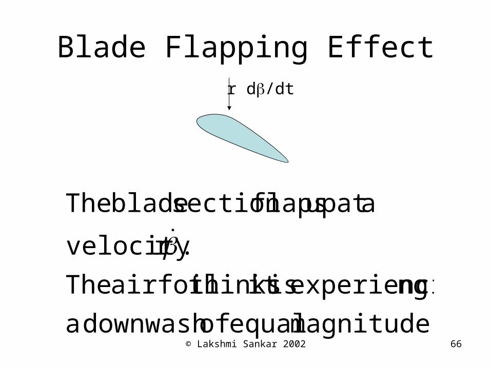
Blade Flapping Effect
magnitude. equal ofdownwash a
ngexperienci isit thinksairfoil The
.rvelocity
aat up flapssection blade The
r d/dt
© Lakshmi Sankar 2002 67
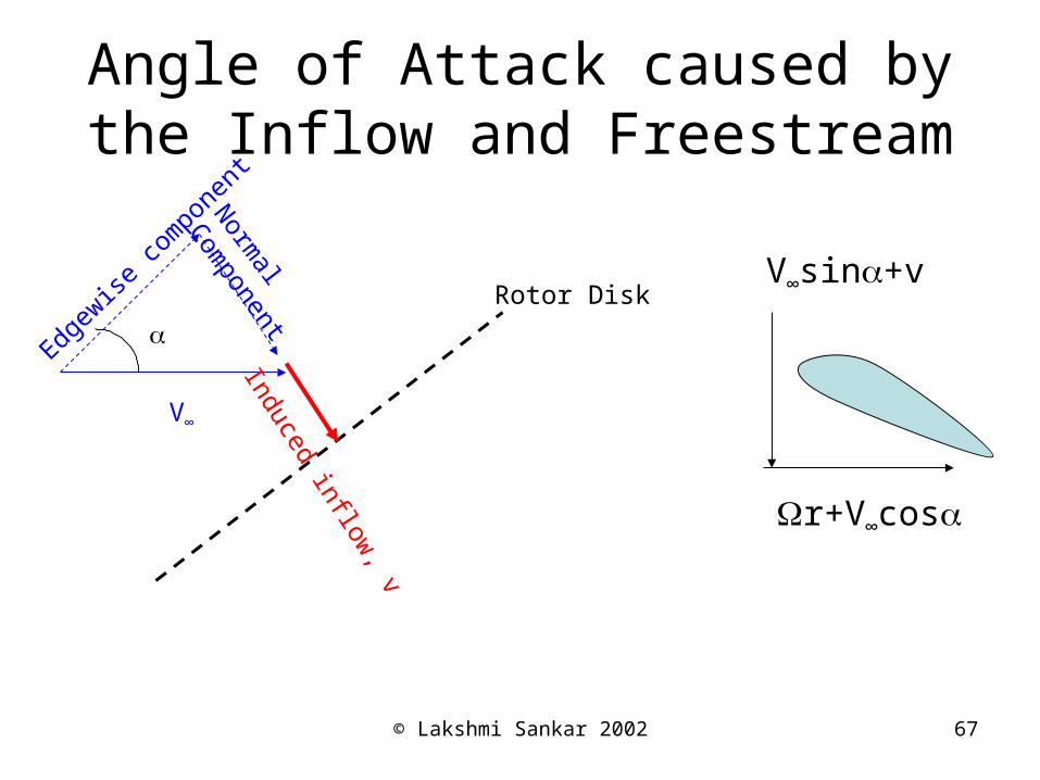
Angle of Attack caused by the Inflow and Freestream
V∞
Rotor Disk
Induced inflow, v
V∞sin+v
r+V∞cos
Edgew
ise co
mpo
nent
Norm
al Com
ponent
© Lakshmi Sankar 2002 68
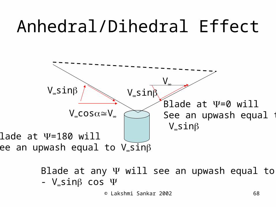
Anhedral/Dihedral Effect
V∞cosV∞
V∞sin
Blade at =180 willSee an upwash equal to V∞sin
V∞sinV∞
Blade at =0 willSee an upwash equal to V∞sin
Blade at any will see an upwash equal to- V∞sin cos
© Lakshmi Sankar 2002 69
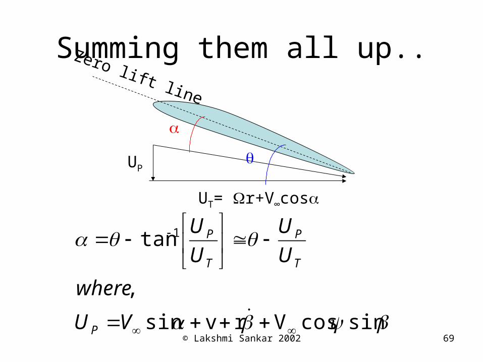
Summing them all up..
UT= r+V∞cos
UP
Zero lift line
sincosVrvsin
,
tan 1
VU
where
U
U
U
U
P
T
P
T
P
© Lakshmi Sankar 2002 70
Small Angle of Attack Assumptions
• The angle of attack a (which is the angle between the freestream and the rotor disk) is small.
• The cyclic and collective pitch angles are all small.
• The coning and flapping angles are all small.
• Cos() = Cos()= Cos() ~ 1• sin() ~ sin() ~ sin() ~
© Lakshmi Sankar 2002 71
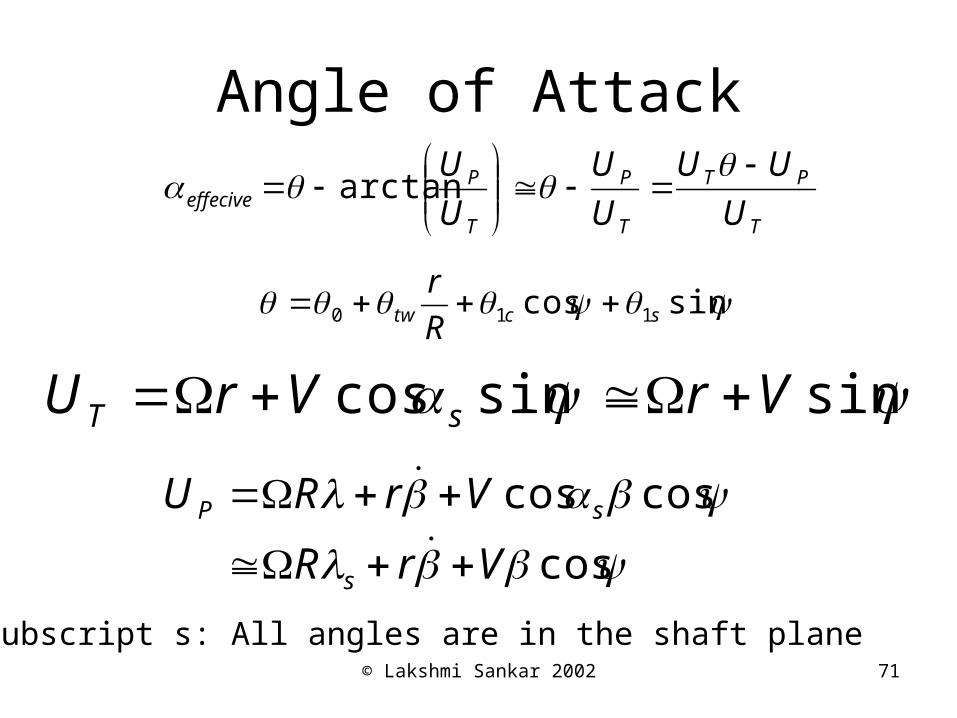
Angle of Attack
T
PT
T
P
T
Peffecive U
UU
U
U
U
U
arctan
sincos 110 sctw R
r
sinsincos VrVrU sT
cos
coscos
VrR
VrRU
s
sP
Subscript s: All angles are in the shaft plane
© Lakshmi Sankar 2002 72
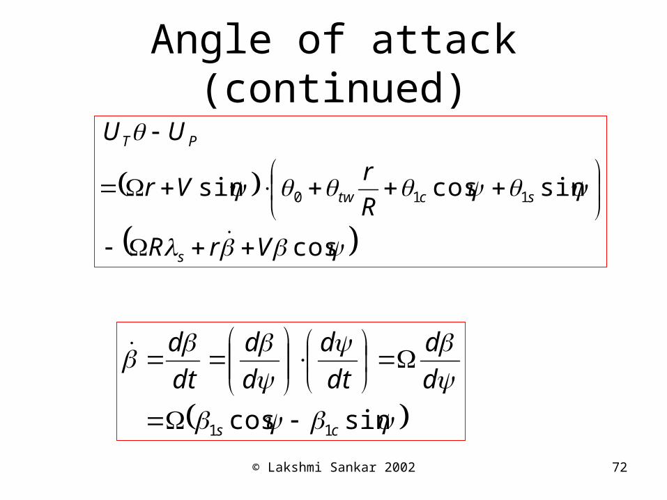
Angle of attack (continued)
cos
sincossin 110
VrR
R
rVr
UU
s
sctw
PT
sincos 11 cs
d
d
dt
d
d
d
dt
d
© Lakshmi Sankar 2002 73
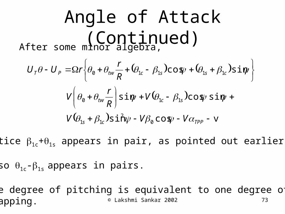
Angle of Attack (Continued)After some minor algebra,
vcossin
sincossin
sincos
02
11
110
11110
TPPcs
sctw
cssctwPT
VVV
VR
rV
R
rrUU
Notice 1c+1s appears in pair, as pointed out earlier.
Also 1c-1s appears in pairs.
One degree of pitching is equivalent to one degree ofFlapping.
© Lakshmi Sankar 2002 74
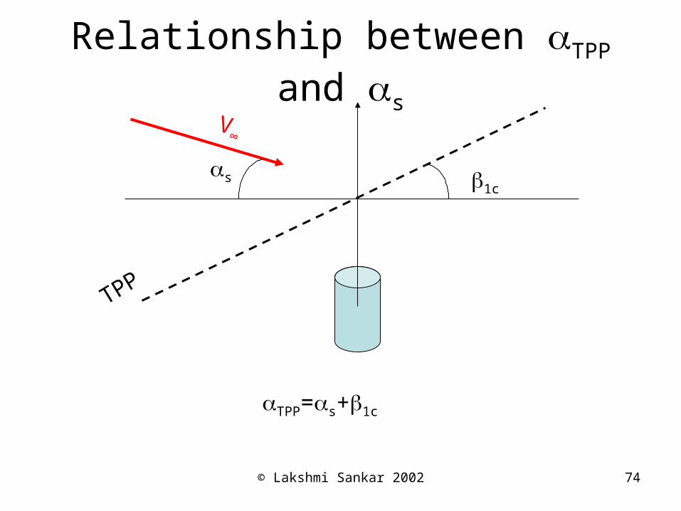
Relationship between TPP and s
TPP=s+1c
V∞
s 1c
TPP
© Lakshmi Sankar 2002 75
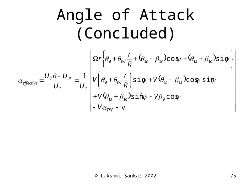
Angle of Attack (Concluded)
v
cossin
sincossin
sincos
1
02
11
110
11110
TPP
cs
sctw
cssctw
TT
PTeffective
V
VV
VR
rV
R
rr
UU
UU
© Lakshmi Sankar 2002 76
Calculation of Sectional Loads
• Once the angle of attack at a blade section is computed as shown in the previous slide, one can compute lift, drag, and pitching moment coefficients.
• This can be done in a number of ways. Modern rotorcraft performance codes (e.g. CAMRAD) give the user numerous choices on the way the force coefficients are computed.
© Lakshmi Sankar 2002 77
Some choices for Computing Sectional Loads as a function of
• In analytical work, it is customary to use Cl=a, Cd=Cd0 = constant, and Cm= Cmo, a constant. Here “a” is the lift curve slope, close to 2.
• In simple computer based simulations using Excel or a program, these loads are corrected for compressibility using Prandtl-Glauert Rule.
• More sophisticated calculations will use C-81 tables, with corrections for the local sweep angle.
© Lakshmi Sankar 2002 78
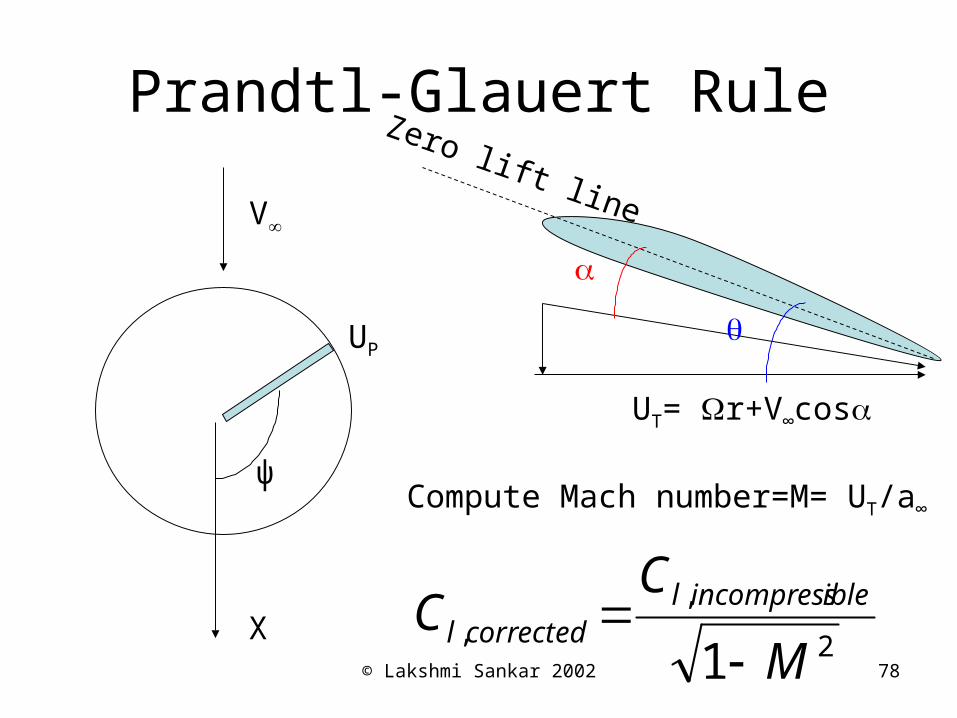
Prandtl-Glauert Rule
X
V∞
ψ
UT= r+V∞cos
UP
Zero lift line
Compute Mach number=M= UT/a∞
2
,,
1 M
CC ibleincompressl
correctedl
© Lakshmi Sankar 2002 79
More accurate ways of computing loads
• In more sophisticated computer programs (e.g. CAMRAD-II, RCAS), a table look up is often used to compute lift, drag, and pitching moments from stored airfoil database.
• These tables only contain steady airfoil loads. Thus, the analysis is quasi-steady.
• In some cases, corrections are made for unsteady aerodynamic effects, and dynamic stall.
• It is important to correct for dynamic stall effects in high speed forward flight to get the vibration levels of the vehicle correct.
© Lakshmi Sankar 2002 80
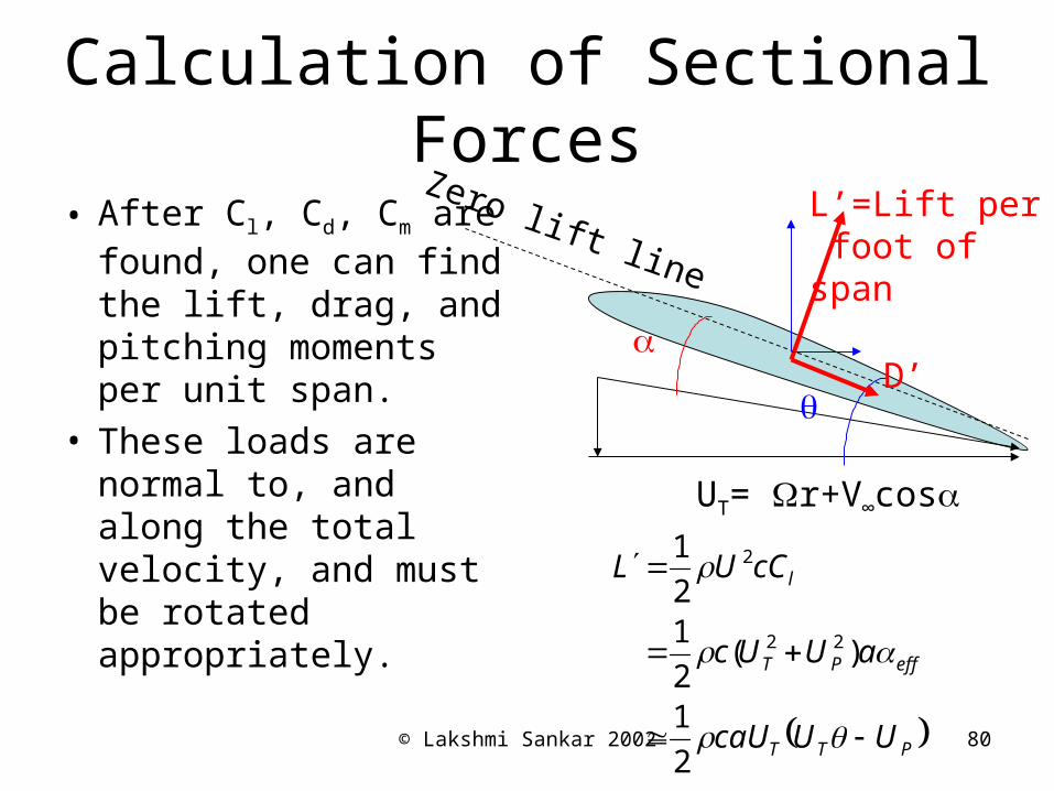
Calculation of Sectional Forces
• After Cl, Cd, Cm are found, one can find the lift, drag, and pitching moments per unit span.
• These loads are normal to, and along the total velocity, and must be rotated appropriately.
UT= r+V∞cos
Zero lift line
L’=Lift per foot ofspan
D’
PTT
effPT
l
UUcaU
aUUc
cCUL
2
1
)(2
12
1
22
2
© Lakshmi Sankar 2002 81
Forward Flight
Integration of Sectional Loads
To get
Total loads
© Lakshmi Sankar 2002 82
Background
• In the previous sections, we discussed how to compute the angle of attack of a typical blade element.
• We also discussed how to compute lift, drag, and pitching moment coefficients.
• We also discussed how to compute sectional lift and drag forces per unit span.
• We mentioned that these loads must be rotated to get components normal to, and along reference plane.
• In this section, we discuss how to integrate these loads.• In computer codes, these integrations are done
numerically.• Analytical integration under simplifying assumptions will
be given here to illustrate the process.
© Lakshmi Sankar 2002 83
Assumptions for Analytical Integration
• c= constant (untapered rotor)
• v = constant (uniform inflow)
• Cd = constant
• Linearly twisted rotor
• No cut out, no tip losses.
© Lakshmi Sankar 2002 84
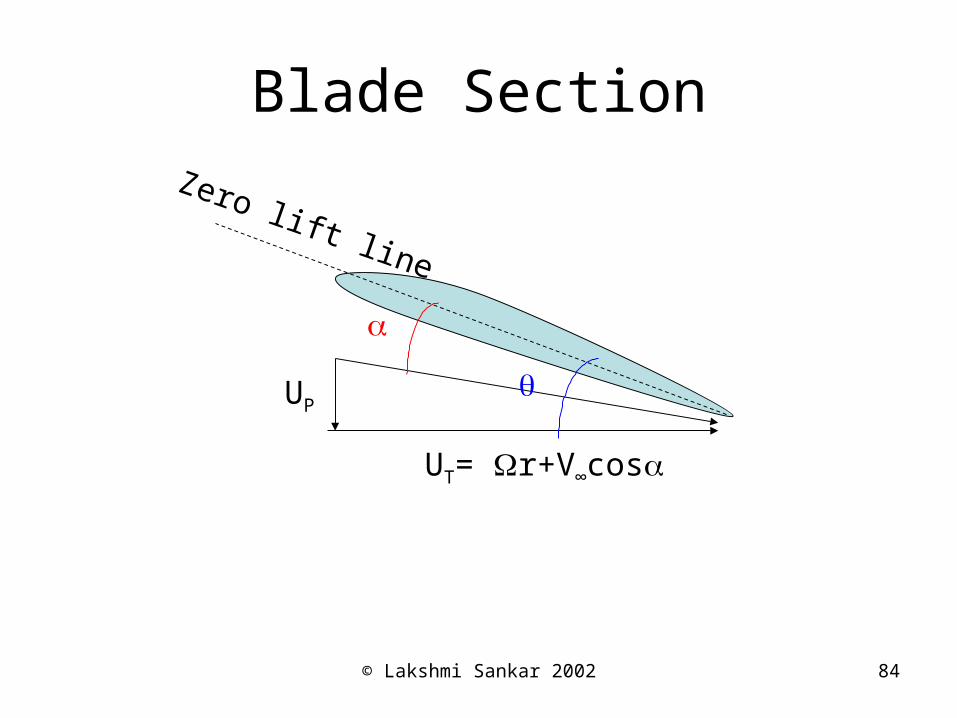
Blade Section
UT= r+V∞cos
UP
Zero lift line
© Lakshmi Sankar 2002 85
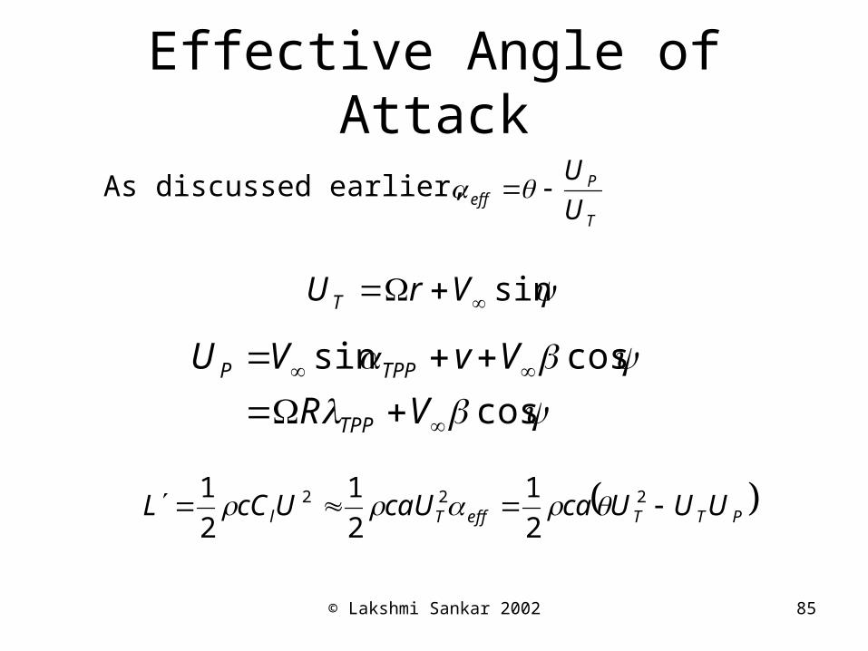
Effective Angle of Attack
As discussed earlier,T
Peff U
U
sin VrUT
cos
cossin
VR
VvVU
TPP
TPPP
PTTeffTl UUUcacaUUcCL 222
2
1
2
1
2
1
© Lakshmi Sankar 2002 86
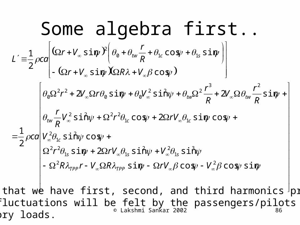
Some algebra first..
sincoscossin
sinsin2sin
cossin
cossin2cossin
sin2sinsin2
2
1
cossin
sincossin
2
1
22
31
2211
22
21
2
112222
23222
0022
0
1102
VrVRVrR
VrVr
V
rVrVR
rR
rV
R
rVrVr
ca
VRVr
R
rVr
caL
TPPTPP
sss
c
cctw
twtw
sctw
Notice that we have first, second, and third harmonics present!These fluctuations will be felt by the passengers/pilots as vibratory loads.
© Lakshmi Sankar 2002 87
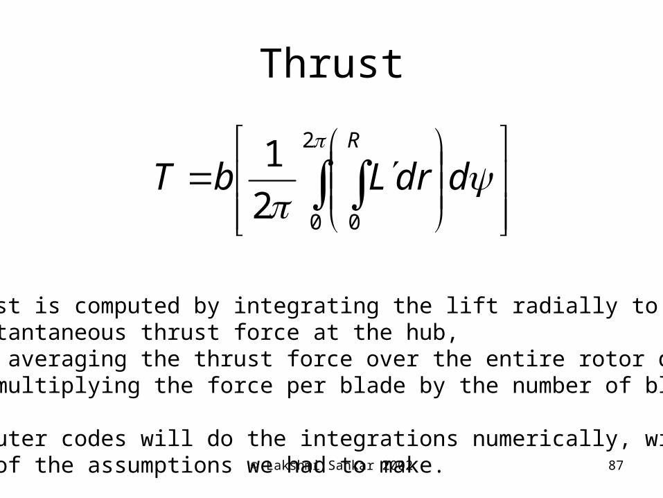
Thrust
2
0 02
1ddrLbT
R
Thrust is computed by integrating the lift radially to get instantaneous thrust force at the hub, then averaging the thrust force over the entire rotor disk,and multiplying the force per blade by the number of blades.
Computer codes will do the integrations numerically, withoutany of the assumptions we had to make.
© Lakshmi Sankar 2002 88
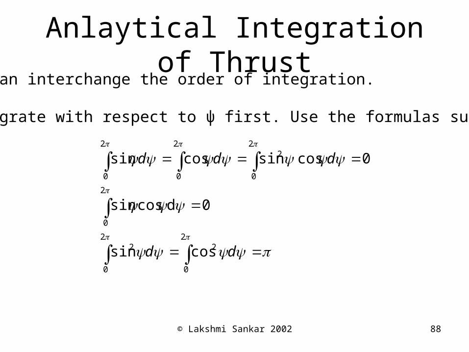
Anlaytical Integration of ThrustWe can interchange the order of integration.
Integrate with respect to ψ first. Use the formulas such as
2
0
22
0
2
2
0
2
0
22
0
2
0
cossin
0dcossin
0cossincossin
dd
ddd
© Lakshmi Sankar 2002 89
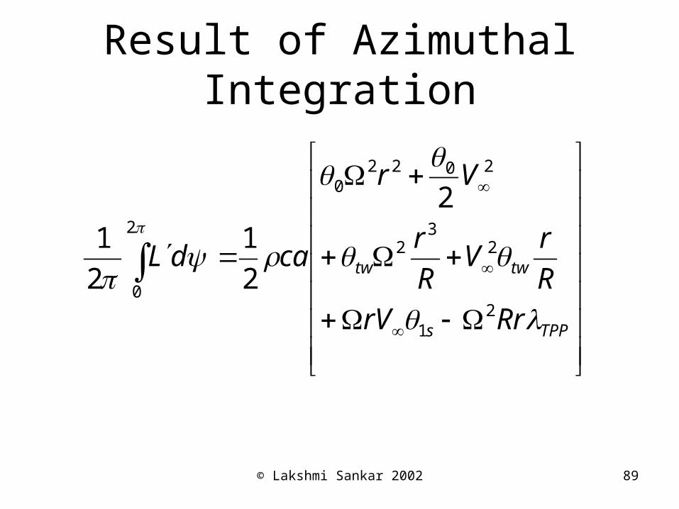
Result of Azimuthal Integration
TPPs
twtw
RrrV
R
rV
R
r
Vr
cadL
21
23
2
20220
2
0
2
2
1
2
1
© Lakshmi Sankar 2002 90
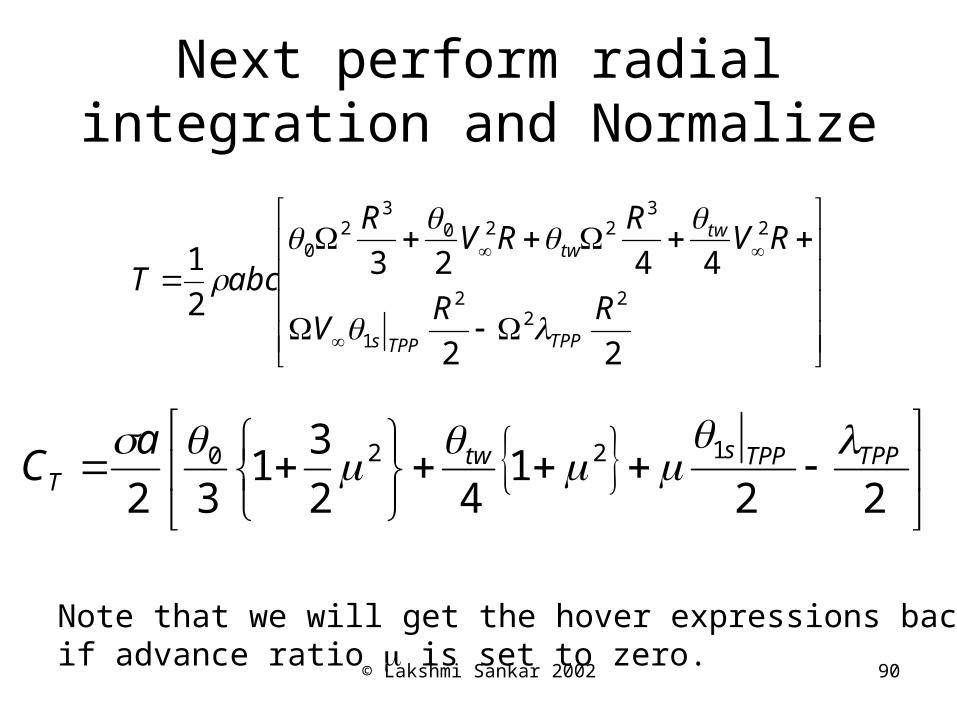
Next perform radial integration and Normalize
22
44232
12
22
1
23
2203
20
RRV
RVR
RVR
abcT
TPPTPPs
twtw
221
42
31
321220 TPPTPPstw
T
aC
Note that we will get the hover expressions back if advance ratio is set to zero.
© Lakshmi Sankar 2002 91
Torque and Power
• We next look at how to compute the instantaneous torque and power on a blade.
• These are azimuthally-averaged to get total torque and total power.
• It is simpler to look at profile and induced components of torque are power separately.
© Lakshmi Sankar 2002 92
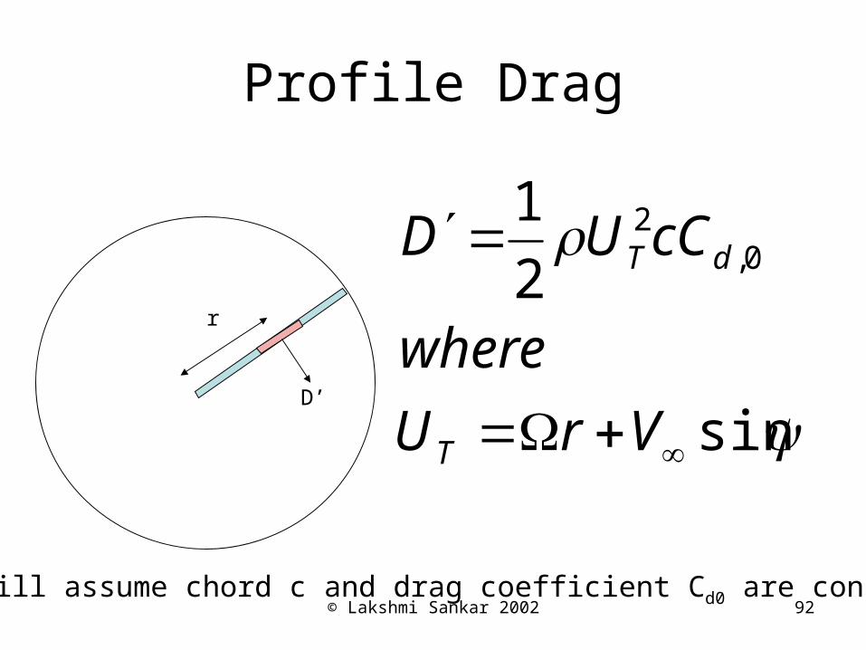
Profile Drag
D’
r
sin
2
10,
2
VrU
where
cCUD
T
dT
We will assume chord c and drag coefficient Cd0 are constant.
© Lakshmi Sankar 2002 93
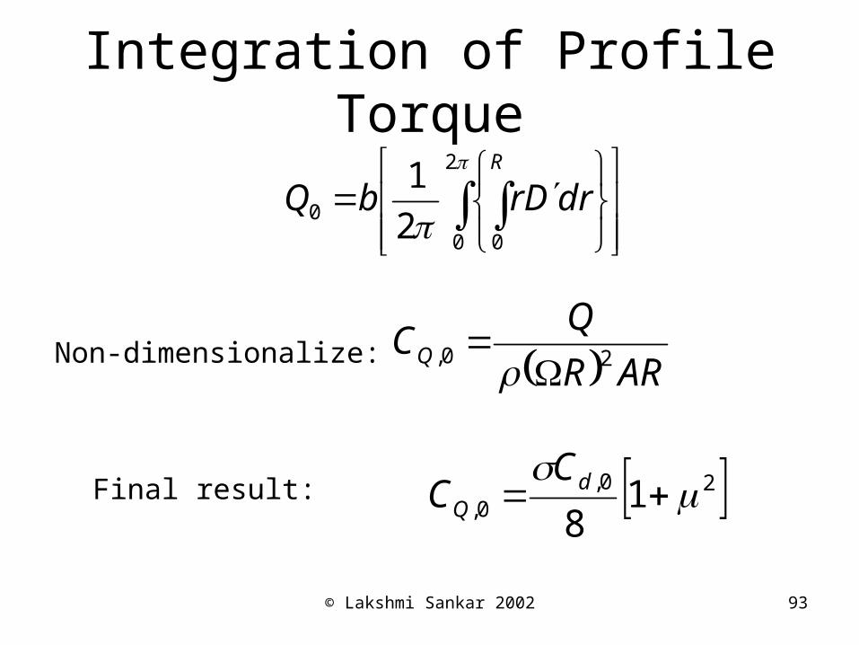
Integration of Profile Torque
2
0 0
0 2
1 R
drDrbQ
ARR
QCQ 20,
Non-dimensionalize:
Final result: 20,0, 1
8
d
Q
CC
© Lakshmi Sankar 2002 94
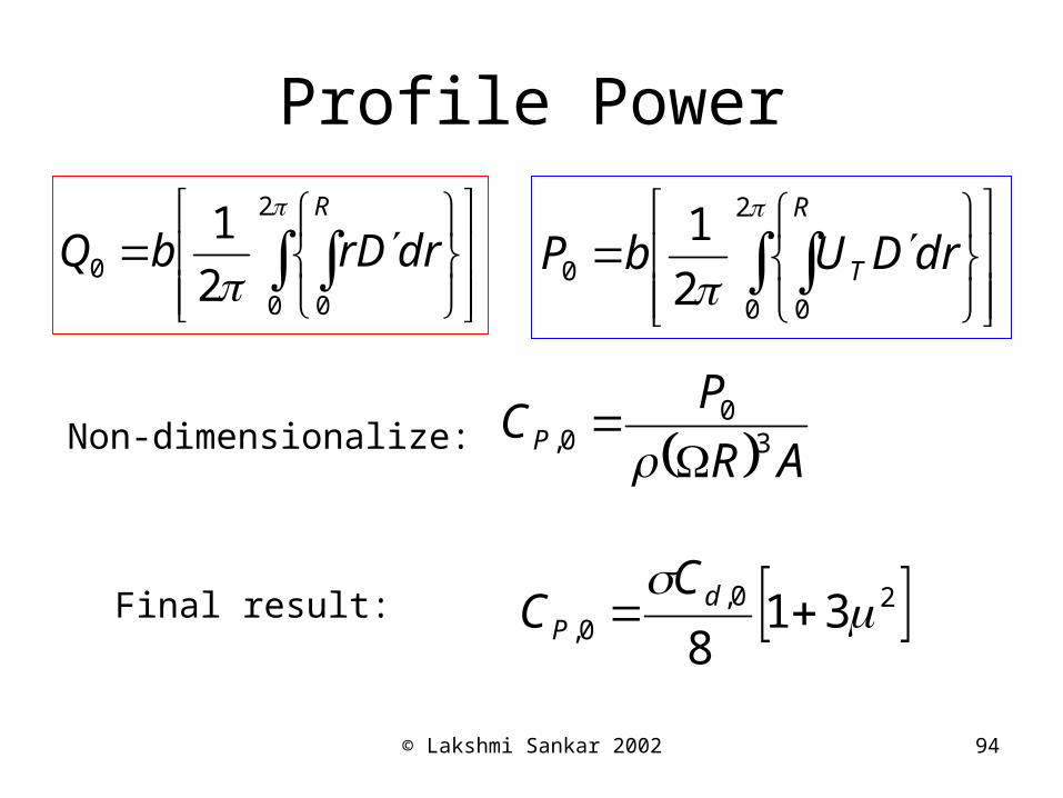
Profile Power
2
0 0
0 2
1 R
drDrbQ
AR
PCP 3
00,
Non-dimensionalize:
Final result: 20,0, 31
8
d
P
CC
2
0 0
0 2
1 R
T drDUbP
© Lakshmi Sankar 2002 95
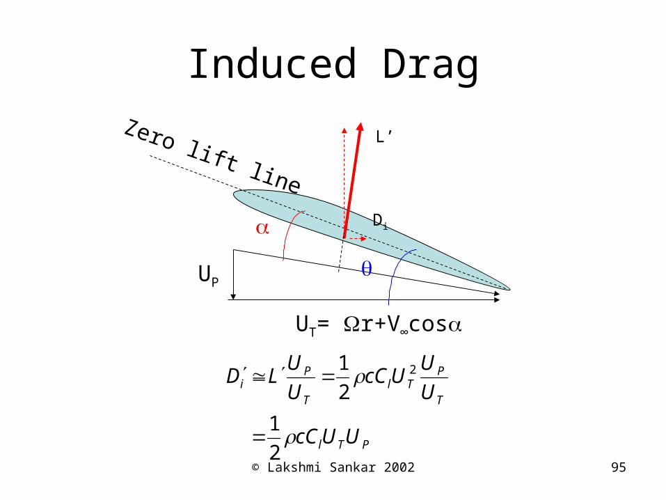
Induced Drag
UT= r+V∞cos
UP
Zero lift line
L’
Di
PTl
T
PTl
T
Pi
UUcC
U
UUcC
U
ULD
2
1
2
1 2
© Lakshmi Sankar 2002 96
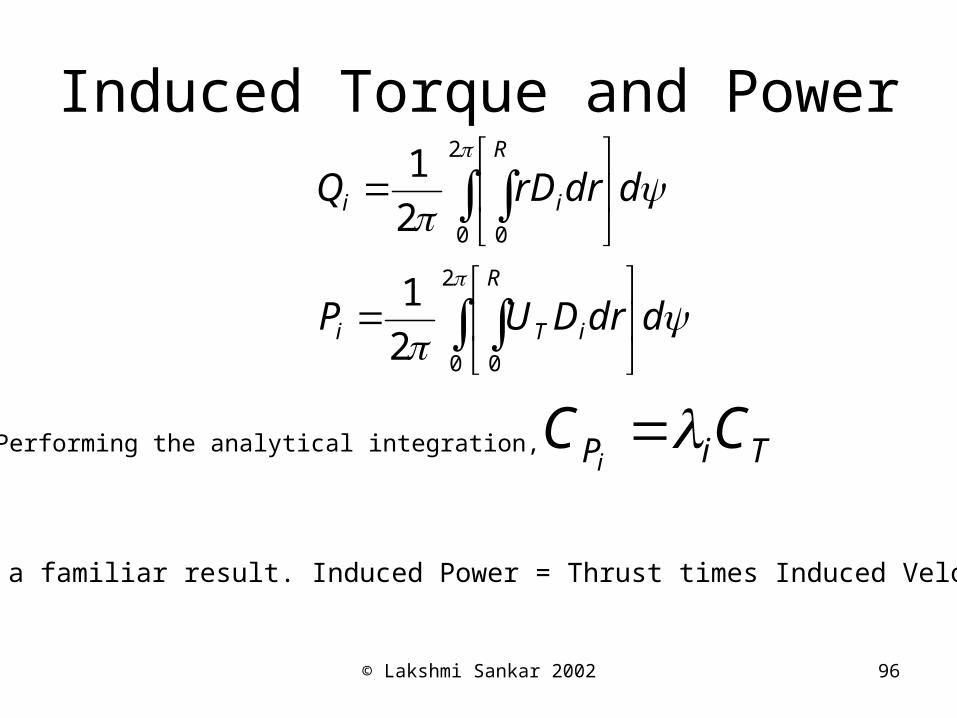
Induced Torque and Power
2
0 0
2
0 0
2
1
2
1
ddrDUP
ddrrDQ
R
iTi
R
ii
Performing the analytical integration, TiP CCi
This is a familiar result. Induced Power = Thrust times Induced Velocity!
© Lakshmi Sankar 2002 97
In-Plane Forces
• In addition to thrust, that act normal to the rotor disk (or along the z-axis in the coordinate selected by the user), the blade sections generate in-plane forces.
• These forces must be integrated to get net force along the x- axis. This is called the H-force.
• These forces must be integrated to get net forces along the Y- axis. This is called the Y-force.
• These forces will have inviscid components, and viscous components.
© Lakshmi Sankar 2002 98
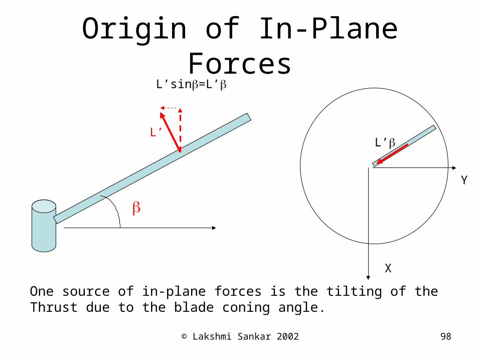
Origin of In-Plane Forces
L’
One source of in-plane forces is the tilting of theThrust due to the blade coning angle.
L’sin=L’
L’
X
Y
© Lakshmi Sankar 2002 99
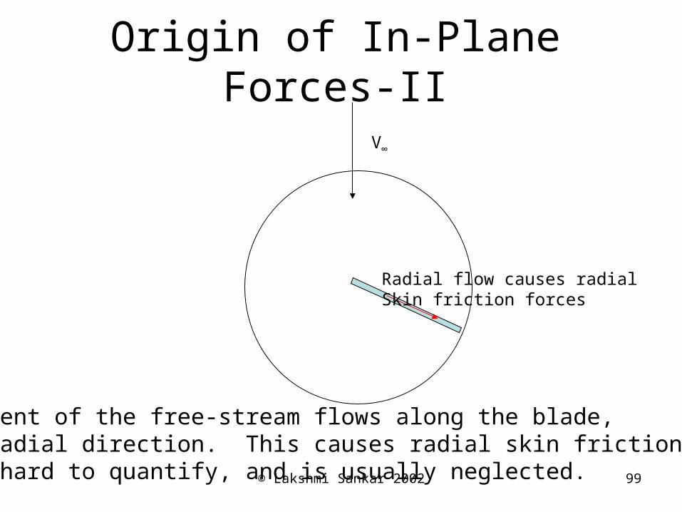
Origin of In-Plane Forces-II
V∞
A component of the free-stream flows along the blade, in the radial direction. This causes radial skin friction forces. This is hard to quantify, and is usually neglected.
Radial flow causes radialSkin friction forces
© Lakshmi Sankar 2002 100
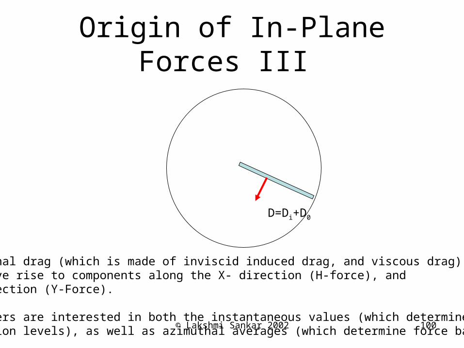
Origin of In-Plane Forces III
D=Di+D0
Sectional drag (which is made of inviscid induced drag, and viscous drag)Can give rise to components along the X- direction (H-force), andY- direction (Y-Force).
Engineers are interested in both the instantaneous values (which determineVibration levels), as well as azimuthal averages (which determine force balance).
© Lakshmi Sankar 2002 101
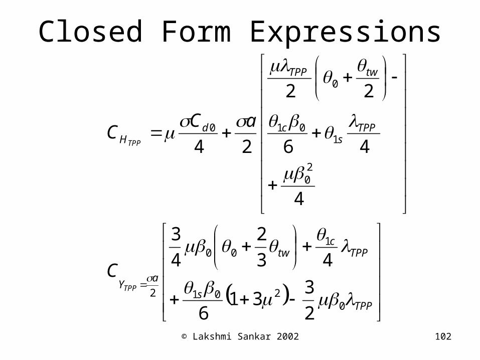
Closed Form Expressions for CH and CY
• Under our assumptions of constant chord, linear twist, linear aerodynamics, and uniform inflow, these forces may be integrated radially, and averaged azimuthally.
• The H- forces and the Y- forces are non-dimensionalized the same way thrust is non-dimensionalized.
• Many text books (e.g. Leishman, Prouty) give exact expressions for these coefficients.
© Lakshmi Sankar 2002 102
Closed Form Expressions
TPPs
TPPc
tw
aY
TPPs
c
twTPP
dH
TPP
TPP
C
aCC
0201
100
2
20
101
0
0
2
331
6
43
2
4
3
4
46
22
24
© Lakshmi Sankar 2002 103
Forward Flight
Calculation of Blade Flapping Dynamics
© Lakshmi Sankar 2002 104
Background
• In the previous sections, we developed expressions for sectional angle of attack, sectional loads, total thrust, torque, power, H-force and Y-force.
• These equations assumed that the blade flapping dynamics a priori.
• The blade flapping coefficients are determined by solving the ODE that covers flapping.
© Lakshmi Sankar 2002 105
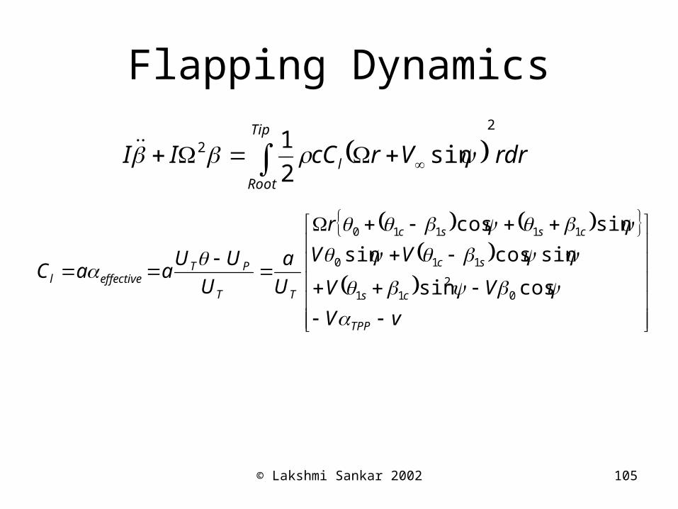
Flapping Dynamics
rdrVrcCIITip
Root
l
2
2 sin2
1
vV
VV
VV
r
U
a
U
UUaaC
TPP
cs
sc
cssc
TT
PTeffectivel
cossin
sincossin
sincos
02
11
110
11110
© Lakshmi Sankar 2002 106
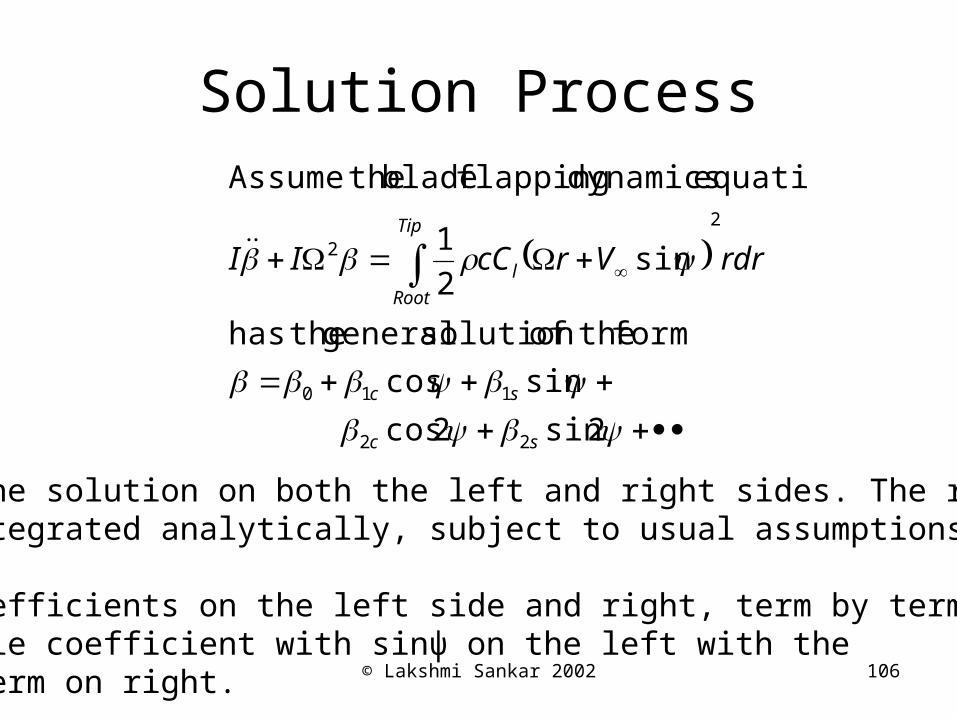
Solution Process
2sin2cos
sincos
form theofsolution general thehas
sin2
1
equation dynamics flapping blade theAssume
22
110
2
2
sc
sc
Tip
Root
l rdrVrcCII
Plug in the solution on both the left and right sides. The right sideCan be integrated analytically, subject to usual assumptions.
Equate coefficients on the left side and right, term by term.For example coefficient with sinψ on the left with thesimilar term on right.
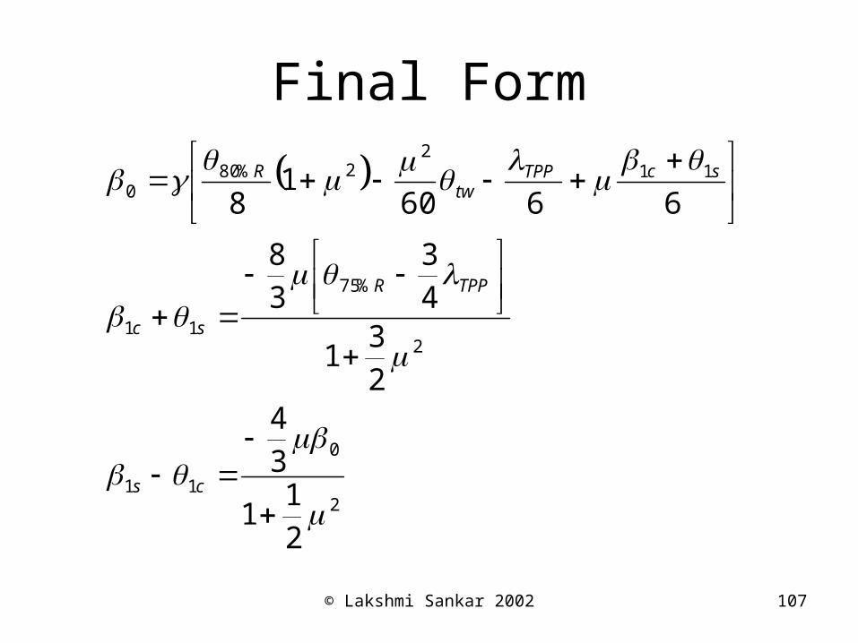
© Lakshmi Sankar 2002 107
Final Form
2
0
11
2
%75
11
112
2%800
2
11
3
42
31
4
3
3
8
66601
8
cs
TPPR
sc
scTPPtw
R
© Lakshmi Sankar 2002 108
Level Flight
Calculation of Trim Conditions
Including
Fuselage Aerodynamics
© Lakshmi Sankar 2002 109
Background
• By trim conditions we mean the operating conditions of the entire vehicle, including the main rotor, tail rotor, and the fuselage, needed to maintain steady level flight.
• The equations are all non-linear, algebraic, and coupled.
• An iterative procedure is therefore needed.
© Lakshmi Sankar 2002 110
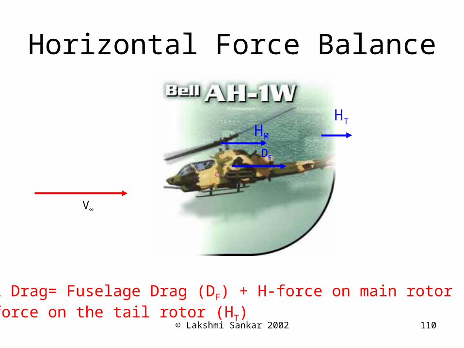
Horizontal Force Balance
V∞
DF
HM
HT
Total Drag= Fuselage Drag (DF) + H-force on main rotor (HM)+ H-force on the tail rotor (HT)
© Lakshmi Sankar 2002 111
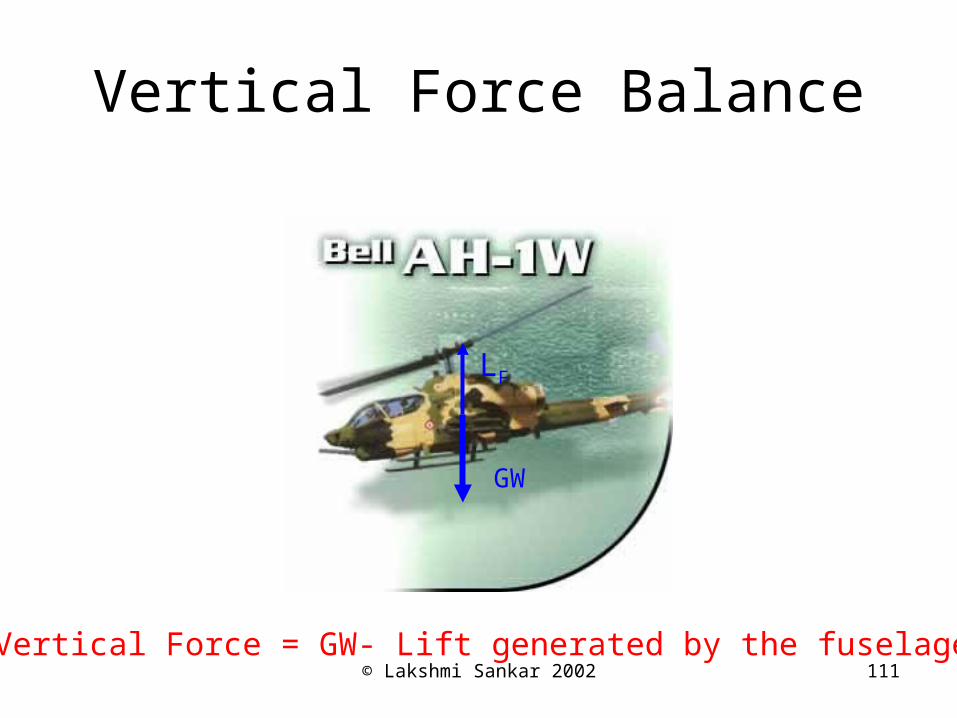
Vertical Force Balance
LF
GW
Vertical Force = GW- Lift generated by the fuselage, LF
© Lakshmi Sankar 2002 112
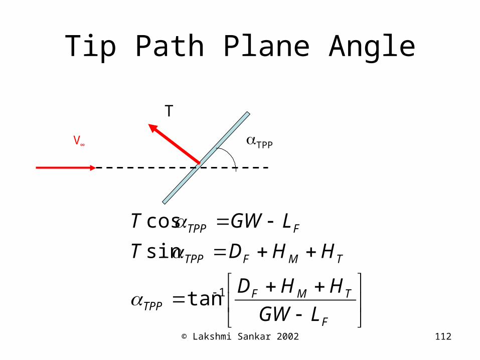
Tip Path Plane Angle
V∞ TPP
T
F
TMFTPP
TMFTPP
FTPP
LGW
HHD
HHDT
LGWT
1tan
sin
cos
© Lakshmi Sankar 2002 113
Fuselage Lift and Drag
• These are functions of the fuselage geometry, and its attitude (or angle of attack).
• This information is currently obtained from wind tunnel studies, and stored as a data-base in computer codes.
© Lakshmi Sankar 2002 114
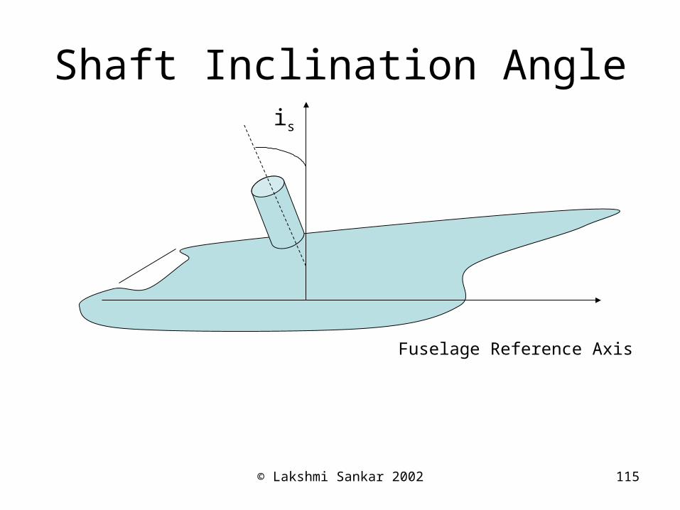
Fuselage Angle of Attack
• Extracted from – Tip path angle – Blade flapping dynamics – Downwash felt by the fuselage from the main
rotor – Shaft inclination angle.
© Lakshmi Sankar 2002 115
Shaft Inclination Angle
Fuselage Reference Axis
is
© Lakshmi Sankar 2002 116
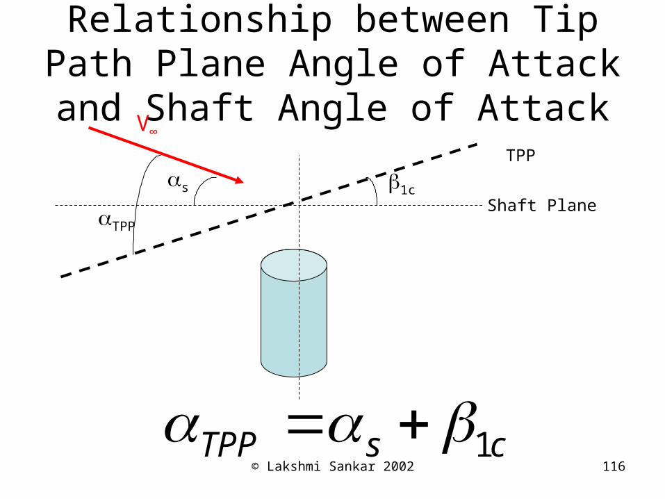
Relationship between Tip Path Plane Angle of Attack and Shaft
Angle of AttackTPP
Shaft Plane
V∞
s 1c
TPP
csTPP 1
© Lakshmi Sankar 2002 117
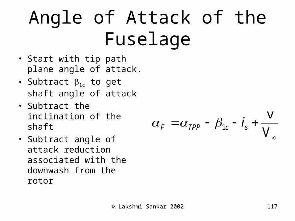
Angle of Attack of the Fuselage
• Start with tip path plane angle of attack.
• Subtract 1c to get shaft angle of attack
• Subtract the inclination of the shaft
• Subtract angle of attack reduction associated with the downwash from the rotor
V
v1 scTPPF i
© Lakshmi Sankar 2002 118
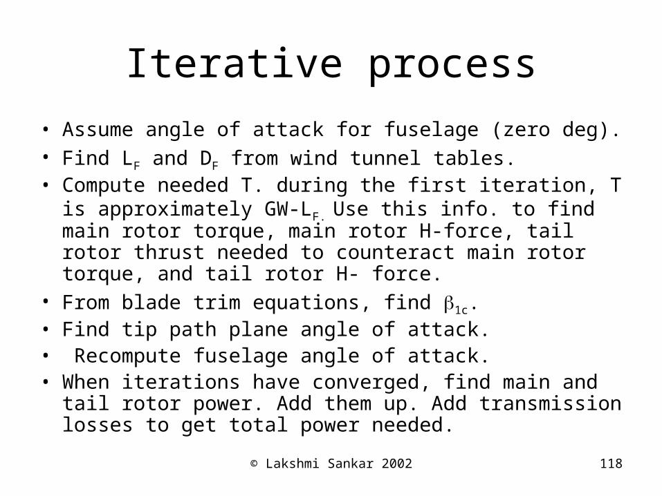
Iterative process
• Assume angle of attack for fuselage (zero deg).• Find LF and DF from wind tunnel tables.• Compute needed T. during the first iteration, T is
approximately GW-LF. Use this info. to find main rotor torque, main rotor H-force, tail rotor thrust needed to counteract main rotor torque, and tail rotor H- force.
• From blade trim equations, find 1c.• Find tip path plane angle of attack.• Recompute fuselage angle of attack.• When iterations have converged, find main and tail rotor
power. Add them up. Add transmission losses to get total power needed.
© Lakshmi Sankar 2002 119
Autorotation in Forward Flight
• The calculations described for steady level flight can be modified to handle autorotative descent in forward flight.
• Power needed is supplied by the time rate of loss in potential energy.
© Lakshmi Sankar 2002 120
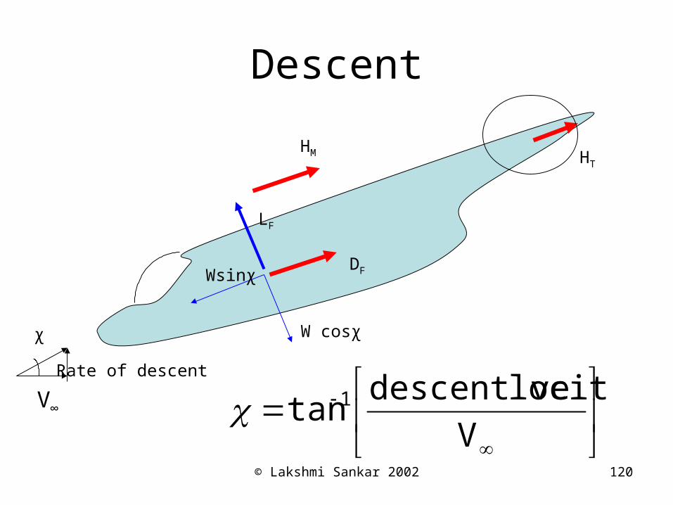
Descent
V∞
Wsinχ
W cosχ
Rate of descent
χ
V
locitydescent vetan 1
DF
HT
HM
LF
© Lakshmi Sankar 2002 121
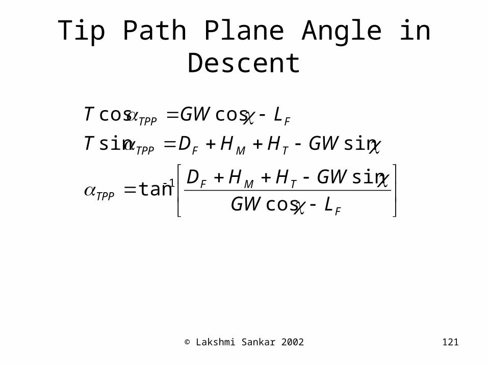
Tip Path Plane Angle in Descent
F
TMFTPP
TMFTPP
FTPP
LGW
GWHHD
GWHHDT
LGWT
cos
sintan
sinsin
coscos
1
© Lakshmi Sankar 2002 122
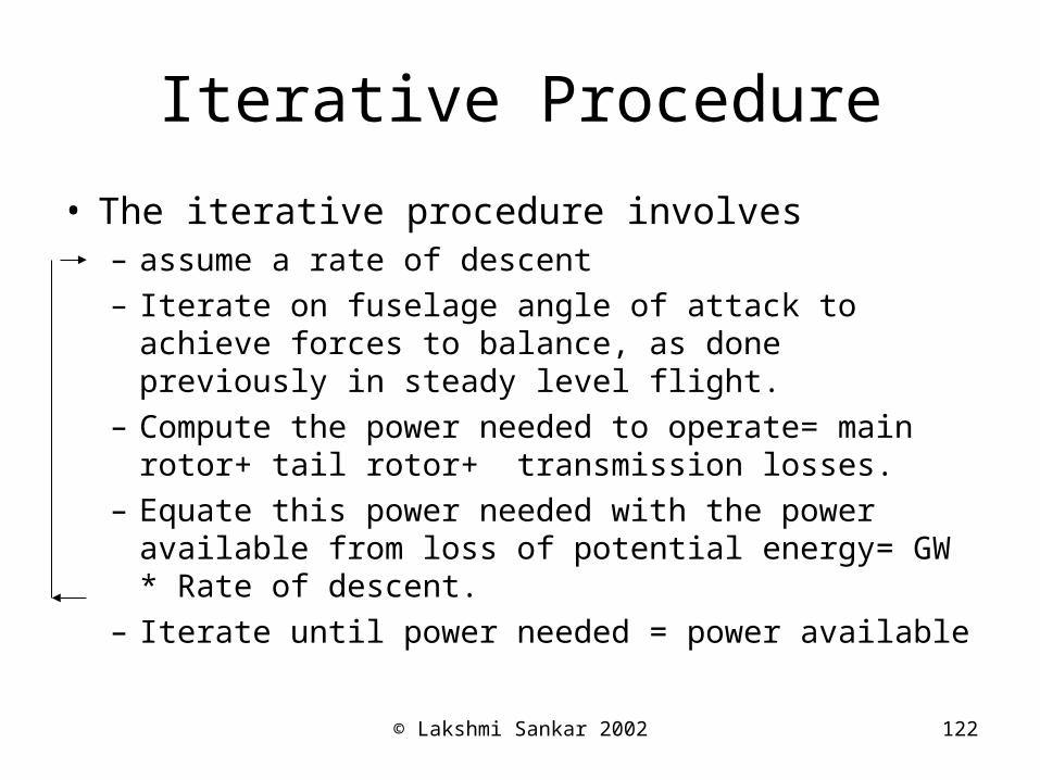
Iterative Procedure
• The iterative procedure involves – assume a rate of descent– Iterate on fuselage angle of attack to achieve forces
to balance, as done previously in steady level flight.– Compute the power needed to operate= main rotor+
tail rotor+ transmission losses.– Equate this power needed with the power available
from loss of potential energy= GW * Rate of descent.– Iterate until power needed = power available
Recommended