Karazin Kharkiv National University

Department of Physics and Technology

Technische Universitat Darmstadt

Institut fur Kernphysik

Spatial Autocorrelation Function of WaveFunctions in a Chaotic Microwave Billiard

Diploma Thesis

Maksim Miski-Oglu

Darmstadt 2002

Dedicated to my beloved wife Nataly

Abstract In the present diploma thesis an experimental test of the theoretical

prediction about the asymptotical behavior of a spatial autocorrelation function for

quantum systems, the classical counterpart of which is ergodic, has been carried

out. The basis of the experimental verification is the analogy between the

Schrödinger equation for a point like-particle confined in a hard-wall potential and

the Helmholtz equation for a quasi two-dimensional microwave resonator. The test

was made for the eigenfunctions of a microwave Sinai billiard. For the

experimental determination of the electromagnetic field intensity, which

corresponds to the eigenfunctions of the microwave resonator, the perturbation

body technique was used. For the extraction of the electrical field strength from the

electromagnetic field intensity a field reconstruction procedure was specially

developed within the framework of the diploma thesis. Good agreement with

theory was obtained for an averaged over all directions of separating vector

autocorrelation function. The autocorrelation function for different direction of

separating vectors shows a more complicated behavior than predicted.

2

Анотація Дана дипломна робота – це експериментальна перевірка

теоретичного передбачення асимптотичної поведінки просторової

автокореляційної функції для квантових систем чиї класичні аналоги є

ергодичні. Основа цієї перевірки полягає у тому, що існує повна

аналогія між рівнянням Шредінгера для вільної частинки у двомірній

потенційній ямі та рівнянням Гельмгольца у випадку квазідвомірного

мікрохвильового резонатора. У цій роботі була досліджена поведінка

автокореляційної функції у випадку мікрохвильового більярда Сіная.

Для спостереження інтенсивності електромагнітного поля, котра

відповідає власним функціям резонатора, було застосовано метод

збурюючого тіла. Для знаходження напруженості електричного поля

було спеціально розроблено процедуру реконструкції поля. У випадку

усередненої автокореляційної функції була отримана добра

відповідність теорії з експериментом. Для окремих напрямків

автокореляційна функція виявила більш детальну структуру ніж було

передбачено теорією.

3

Contents

1 Introduction.................................................................................. 5

2 Billiards......................................................................................... 7

2.1 Classical Billiards..................................................................................... 7

2.2 Quantum Billiards .................................................................................... 8

2.3 Microwave Billiards ................................................................................. 9

3 Quantum Autocorrelation Function......................................... 10

4 Experimental Techniques.......................................................... 14

4.1 Maier-Slater Formula ............................................................................. 14

4.2 Positioning Unit...................................................................................... 15

4.3 Microwave Cavity .................................................................................. 18

5 Analysis and Results .................................................................. 20

5.1 Field Reconstruction Procedure ............................................................. 20

5.2 Calculation of the Autocorrelation Functions ........................................ 24

5.3 Results .................................................................................................... 27

6 Conclusion and Outlook ............................................................ 31

References......................................................................................... 32

4

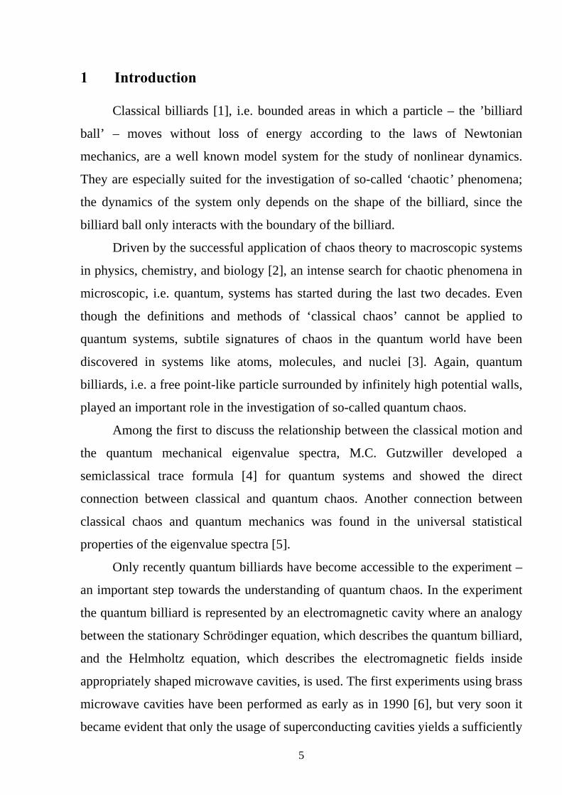
1 Introduction

Classical billiards [1], i.e. bounded areas in which a particle – the ’billiard

ball’ – moves without loss of energy according to the laws of Newtonian

mechanics, are a well known model system for the study of nonlinear dynamics.

They are especially suited for the investigation of so-called ‘chaotic’ phenomena;

the dynamics of the system only depends on the shape of the billiard, since the

billiard ball only interacts with the boundary of the billiard.

Driven by the successful application of chaos theory to macroscopic systems

in physics, chemistry, and biology [2], an intense search for chaotic phenomena in

microscopic, i.e. quantum, systems has started during the last two decades. Even

though the definitions and methods of ‘classical chaos’ cannot be applied to

quantum systems, subtile signatures of chaos in the quantum world have been

discovered in systems like atoms, molecules, and nuclei [3]. Again, quantum

billiards, i.e. a free point-like particle surrounded by infinitely high potential walls,

played an important role in the investigation of so-called quantum chaos.

Among the first to discuss the relationship between the classical motion and

the quantum mechanical eigenvalue spectra, M.C. Gutzwiller developed a

semiclassical trace formula [4] for quantum systems and showed the direct

connection between classical and quantum chaos. Another connection between

classical chaos and quantum mechanics was found in the universal statistical

properties of the eigenvalue spectra [5].

Only recently quantum billiards have become accessible to the experiment –

an important step towards the understanding of quantum chaos. In the experiment

the quantum billiard is represented by an electromagnetic cavity where an analogy

between the stationary Schrödinger equation, which describes the quantum billiard,

and the Helmholtz equation, which describes the electromagnetic fields inside

appropriately shaped microwave cavities, is used. The first experiments using brass

microwave cavities have been performed as early as in 1990 [6], but very soon it

became evident that only the usage of superconducting cavities yields a sufficiently

5

high resolution to allow detailed studies of quantum chaotic phenomena. Such

experiments have been performed at the Institute for Nuclear Physics in Darmstadt

since 1991 and yielded for the first time complete sets of eigenvalues [7].

Information about the dynamics of the system is not only found in the

eigenvalue spectra but also in the distributions and the structure of the

eigenfunctions of the microwave cavity. To test the various theoretical predictions

for the properties and the structure of chaotic eigenfunctions, however, normal

conducting microwave cavities are used. One of the most important features of the

eigenfunctions are the spatial autocorrelations, which asymptotically behave

different for classically integrable and for classically ergodic systems.

The experimental investigation of this connection between the classical

dynamics and the structure of a quantum eigenfunction will be the main topic of

this thesis. After a short introduction and a description of the various types of

billiards – which form the base of the experiment – in chapter 2, the theory, mainly

formulated by Berry [8], is presented in chapter 3. There are only a few

experimental methods which allow the investigation of the electromagnetic field in

a microwave cavity and thus of the wave function of its quantum counterpart. In

this work the perturbation body method – based on theoretical investigations by

Maier and Slater [9] – was used, which originally was invented in accelerator

physics. Despite the fact that the perturbation body method yields only the field

intensity distributions, the achievable high resolution justifies using it for the

investigation of the autocorrelations of field distributions inside microwave

resonators. Nevertheless the measured field intensity patterns have to be processed

further to reconstruct the field distributions itself, which are then used to obtain

autocorrelation functions for billiard systems experimentally. Since a couple of

years, this method is used very successfully in the experimental framework of

quantum chaos experiments [10-13]. It is described in chapter 4 of this work. In

chapter 5 the algorithm that is used to reconstruct the signed field pattern from the

field intensity inside the cavity is described – it has been developed in the context

of this work and is applied for the first time. Also in chapter 5 a comparison

between the theoretical predictions for highly excited modes and the experimental

6

results is done. Although the results presented in this thesis have been achieved

mainly for low lying modes, the agreement between experiment and theory is

remarkable. In chapter 6 the results are summarized and an outlook for further

experiments – aiming to investigate the autocorrelations of the wave functions of

highly excited states and their nodal line patterns – is given.

2 Billiards

In the following chapter the different billiard types are introduced and

discussed. While the classical billiard is commonly used for the analysis of chaos

in conservative systems, the quantum billiard – which can be derived from the

classical billiard – shows also subtle signatures of chaos. In the third part of this

chapter an analog to the quantum billiard, the electromagnetic billiard, which

makes the quantum billiard accessible to the experiment, is discussed.

2.1 Classical Billiards

A classical billiard is a system in which an ideal particle – the billiard ball

with mass m and momentum p moves without loss of energy. The particle only

interacts with the boundary of the billiard, where it is reflected elastically. The

dynamics of this motion only depends on the shape of the boundary and allows for

a classification to regular, chaotic, and mixed systems. To investigate to which

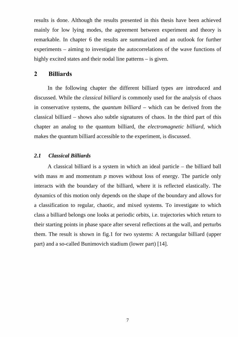
class a billiard belongs one looks at periodic orbits, i.e. trajectories which return to

their starting points in phase space after several reflections at the wall, and perturbs

them. The result is shown in fig.1 for two systems: A rectangular billiard (upper

part) and a so-called Bunimovich stadium (lower part) [14].

7

Fig. 1: Small perturbation of a periodic orbit; the rectangular billiard (upper diagram) is

integrable, while the Bunimovich stadium (lower diagram) shows chaotic behavior.

While the small perturbation of the periodic orbit in the case of the

rectangular billiard leads to linearly diverging orbits – it is therefore considered to

be a regular system – it leads to exponentially diverging orbits in the case of the

Bunimovich stadium, which is a chaotic system. The latter leads to the phase space

being covered ergodically and also reflects itself in the fact that the equations of

motion are not integrable [2].

2.2 Quantum Billiards

A billiard can also be treated in the context of quantum mechanics. In this

case one has to solve the Schrödinger equation for a point-like particle with mass

, momentum , and energy m kpr

hr

⋅= mkE 2/22h= confined to a hard-wall

potential which is shaped according to the form of the classical billiard. The

Schrödinger equation has the form

ψψψψ ⋅=⋅=Δ−=mkE

mH

22

222 hh), (1)

8

where H)

is the Hamilton operator with its eigenfunctions ψ and its eigenvalues E.

This equation is a differential equation which has to be solved with Dirichlet

boundary conditions:

0=wallψ . (2)

As solutions for this equation one finds discrete eigenvalues and

eigenfunctions

nk

nψ [15].

The term ‘chaos’ defined in a classical context as sketched in chapter 2.1 is

not applicable to the quantum billiard, since it is based on looking at small changes

from the initial conditions. Due to the uncertainty relation slight changes in initial

conditions, however, are not an appropriate concept in quantum physics. Quantum

chaos can therefore only be present in the properties of the eigenvalues and

eigenfunctions. According to Berry one should speak only of phenomenological

quantumchaology rather than of quantum chaos [16]. Nevertheless generic

signatures of chaos can be found in the statistical properties of the eigenvalue

spectra [5], where the theoretical predictions are restricted to the semiclassical

regime, i.e. to highly excited states. It is therefore absolutely necessary to use

spectra with a sufficient number of eigenvalues to test these predictions. This can

be achieved by using superconducting microwave cavities [7,17].

2.3 Microwave Billiards

To investigate quantum billiards in an experiment it is necessary to ensure

that the system is described by equation (1) with boundary condition (2).

Consequently, it is not strictly necessary to use real quantum systems. As an

analog system flat microwave cavities can be used in the experiment. The electric

field inside an arbitrary microwave resonator is described by the vectorial

Helmholtz equation

)()( 2

2

rEc

rE rrrr ωεμ−=Δ (3)

for the electric field with Dirichlet boundary conditions

9

0)(tan

rrr=

wallrE (4)

for the tangential electric field )(tan rE rr at the ideally conducting walls. Here c is

the velocity of light, ε and μ are the permittivity and the permeability,

respectively, ω is connected to the eigenfrequencies f of the microwave resonator

by fπω 2= . In contrast to the scalar eigenfunctions ψ of the quantum

mechanical problem this is in general a vectorial equation with vectorial solutions

Er

. Nevertheless, if a flat resonator of height is investigated below an upper

frequency only transverse magnetic modes (TM modes) exist and

the electric field inside the resonator can be written as

d

d2c /=fcritical

zz eyxEE rrr⋅== ),(φ (5)

using a scalar function φ , which depends on x and y. Below the

Helmholtz equation then turns out to be a scalar equation:

criticalf

),(),( 2

2

yxc

yx φωεμφ −=Δ . (6)

Since the form of the scalar equation (6) is identical to that of the Schrödinger

equation (1) with the same boundary condition (2) there is a one-to-one

correspondence between the eigenvalues of the Schrödinger and those of the

Helmholtz equation:

c

mE nn ωεμ↔22h

. (7)

This analogy can of course be extended to the eigenfunctions of the Schrödinger

equation and of the Helmholtz equation and is the basis of this thesis.

3 Quantum Autocorrelation Function

In the following chapter a short description of the autocorrelation function of

quantum eigenfunctions is given. The various predictions for eigenfunctions in the

semiclassical regime are presented and their observability in an experiment is

discussed. The main focus of such investigations are again the connections

10

between the dynamics of the classical and the corresponding quantum system – i.e.

quantum chaos.

The behavior of a quantum mechanical system in the semiclassical limit

strongly depends on the ergodic properties of the corresponding classical system.

In particular, the eigenfunctions semiclassically reflect the phase space structure of

the classical system and therefore depend strongly on whether the classical system

is chaotic or regular. The distribution of amplitudes of an eigenfunction of a

quantum mechanical system whose classical limit is chaotic becomes Gaussian in

the semiclassical limit [18], and numerical studies support this conjecture, see e.g.

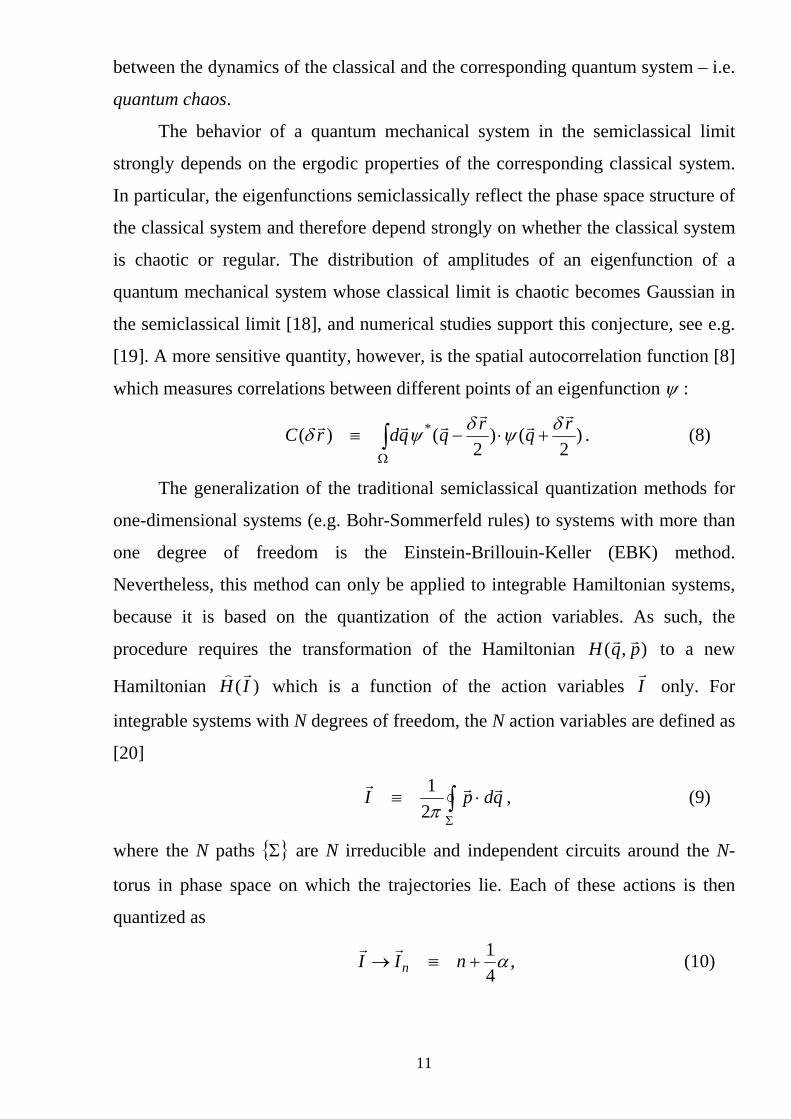
[19]. A more sensitive quantity, however, is the spatial autocorrelation function [8]

which measures correlations between different points of an eigenfunction ψ :

)2

()2

()( * rqrqqdrCr

rr

rrr δψδψδ +⋅−≡ ∫Ω

. (8)

The generalization of the traditional semiclassical quantization methods for

one-dimensional systems (e.g. Bohr-Sommerfeld rules) to systems with more than

one degree of freedom is the Einstein-Brillouin-Keller (EBK) method.

Nevertheless, this method can only be applied to integrable Hamiltonian systems,

because it is based on the quantization of the action variables. As such, the

procedure requires the transformation of the Hamiltonian ),( pqH rr to a new

Hamiltonian )(IHr)

which is a function of the action variables Ir

only. For

integrable systems with N degrees of freedom, the N action variables are defined as

[20]

∫Σ

⋅≡ qdpI rrr

π21 , (9)

where the N paths { are N irreducible and independent circuits around the N-

torus in phase space on which the trajectories lie. Each of these actions is then

quantized as

}Σ

,41α+≡→ nII n

rr (10)

11

where the are integers (n ...,2,1,0=n ) and the numbers α are the Maslov

indicies [21] which are related to the topological structure of the torus in phase

space.

In 1932, Wigner [22], introduced a phase-space distribution function

),( pqW corresponding to a quantum state )(qψ . For systems with N degrees of

freedom this quantity is defined by the N-fold integral

)2

()2

()exp(),( * rqrqrpiXdpqWr

rr

r

h

rrrrr δψδψδ

+⋅−⋅⋅⋅−= ∫ (11)

namely the Fourier transform of the product of ψ and *ψ at positions separated by

, where Xr

),( pqW rr is a quantal generalization of the classical density of points in

phase space. The Wigner function ),( pqW rr is connected to the autocorrelation

function by the following expression:

∫ ⋅⋅⋅= )exp(),()( rpipqWpdqdrC rrrrrrr δδ . (12) Berry [23] showed that the Wigner function ),( pqW rr in a semiclassical

approximation for a quantum system, which has a classically integrable

counterpart, is

]),([)2(

1),( nN IpqIpqWrrwrrr

−≈ δπ

. (13)

The N-dimensional delta function implies that the Wigner function for an

eigenstate is concentrated on the region that an orbit explores over infinite time-

i.e. on the torus.

Berry [8] and Voros [24] proposed to extend this idea to cases where motion

is irregular and consequently not confined to tori. The resulting ‘semiclassical

eigenfunction hypothesis’ can be expressed as follows: Each semiclassical

eigenstate has a Wigner function concentrated on the region explored by a typical

orbit over infinite times.

The stipulation ‘typical’ excludes the measure-zero closed orbits exploring

the lower dimensional region. This hypothesis can be applied to the extreme case

of an ergodic system, whose orbits fill whole energy surfaces in phase space. Each

quantum state corresponds to one energy surface, selected by a quantum condition.

12

What these eigenenergies are is unknown, because nobody has so far discovered

how to associate a wave with an energy surface. For an ergodic system, the

hypothesis gives for the Wigner function representing an eigenstate with energy E

∫ −

−≈

)],([)],([),(

pqHEpdqdpqHEpqW

n

nrrrr

rrrr

δδ . (14)

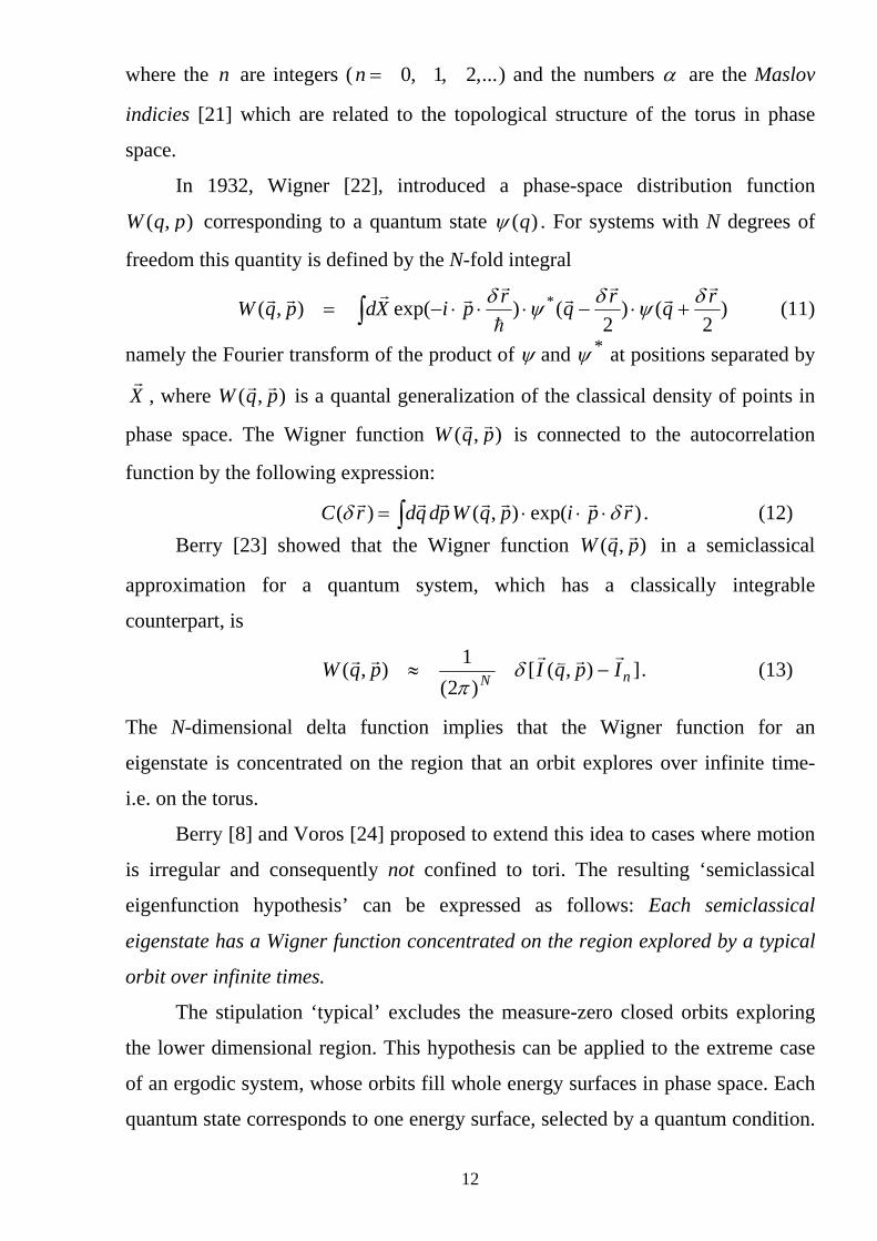
In contrast to equation (13), this is a one-dimensional delta function, reflecting the

fact that ),( pqW is spread over a whole energetic surface.

Inserting expression (14) into the definition of the autocorrelation function

and performing the integration one can obtain a semiclassical expression for the

autocorrelation function in the two-dimensional case

)()( 0 rkJrC rr δδ = , (15)

where k is absolute value of wave vector, is the zeroth order Bessel function.

The fact that the autocorrelation function for two-dimensional systems in the

semiclassical limit only depends on the absolute value of the separating vector

0J

rrδ

means that the semiclassical wave function has a uniform amplitude distribution.

Exactly the same result as expression (15) can be received in a random wave

approach [18], if one represents the semiclassical wave function as a superposition

of plane waves with constant amplitudes and fixed wave lengths but with randomly

oriented wave vectors:

∑ ⋅⋅≈j

kqieqrrr)(ψ . (16)

This model is commonly used for description of chaotic quantum systems. This

model has just recently been employed to demonstrate the close connections

between percolation theory and the structure of eigenstates of quantum chaotic

system [25] – a fact that should be observable with the experimental techniques

developed in the context of the thesis and which will be discussed further in

chapter 6.

13

4 Experimental Techniques

To determine the electromagnetic field intensity distribution, which

corresponds to the quantum wave function, in a microwave billiard, a perturbation

body technique has been used, which was developed and successfully applied in

the context of accelerator physics. In the following chapter the central formula of

the perturbation body method – the Maier-Slater formula – is introduced. In the

chapter 4.2 the positioning unit is described and then the microwave cavity used

for the experiments.

4.1 Maier-Slater Formula

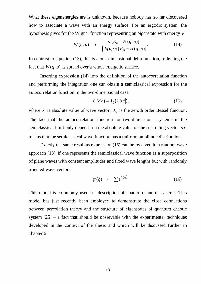
The shift of the resonant frequency caused by perturbing the electromagnetic

field inside a cavity with a small metallic body is given by the Maier-Slater

formula [9]

( )),(),(),( 22

210 yxBcyxEcfyxf

rr⋅−⋅⋅=∂ , (17)

where is the resonant frequency of the unperturbed cavity, 0f Br

is the magnetic

field and Er

is the electric field at the location of the perturbation body and the

constants c1 and c2 are fully determined by the size and shape, e.g. the geometry of

the perturbation body. These constants may dramatically differ in their strength for

the electric and the magnetic field. If we change the location of a metallic

perturbation body in the cavity and record the shift of the resonant frequency for

each point, we can obtain a two-dimensional image of a combination of 2Er

and 2Br

, according to (17), inside the cavity.

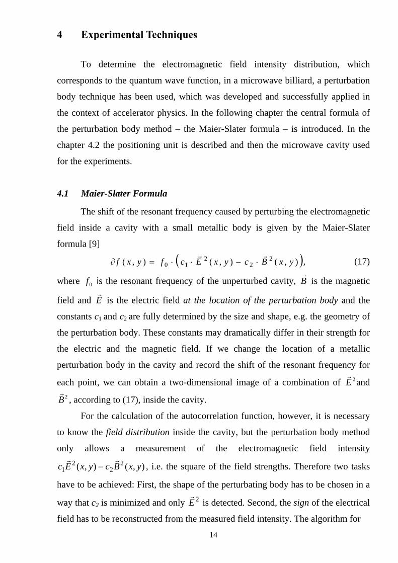
For the calculation of the autocorrelation function, however, it is necessary

to know the field distribution inside the cavity, but the perturbation body method

only allows a measurement of the electromagnetic field intensity

, i.e. the square of the field strengths. Therefore two tasks

have to be achieved: First, the shape of the perturbating body has to be chosen in a

way that c2 is minimized and only

),(),( 22

21 yxBcyxEc

rr−

2Er

is detected. Second, the sign of the electrical

field has to be reconstructed from the measured field intensity. The algorithm for

14

1

2 3

200 mm

20 mm

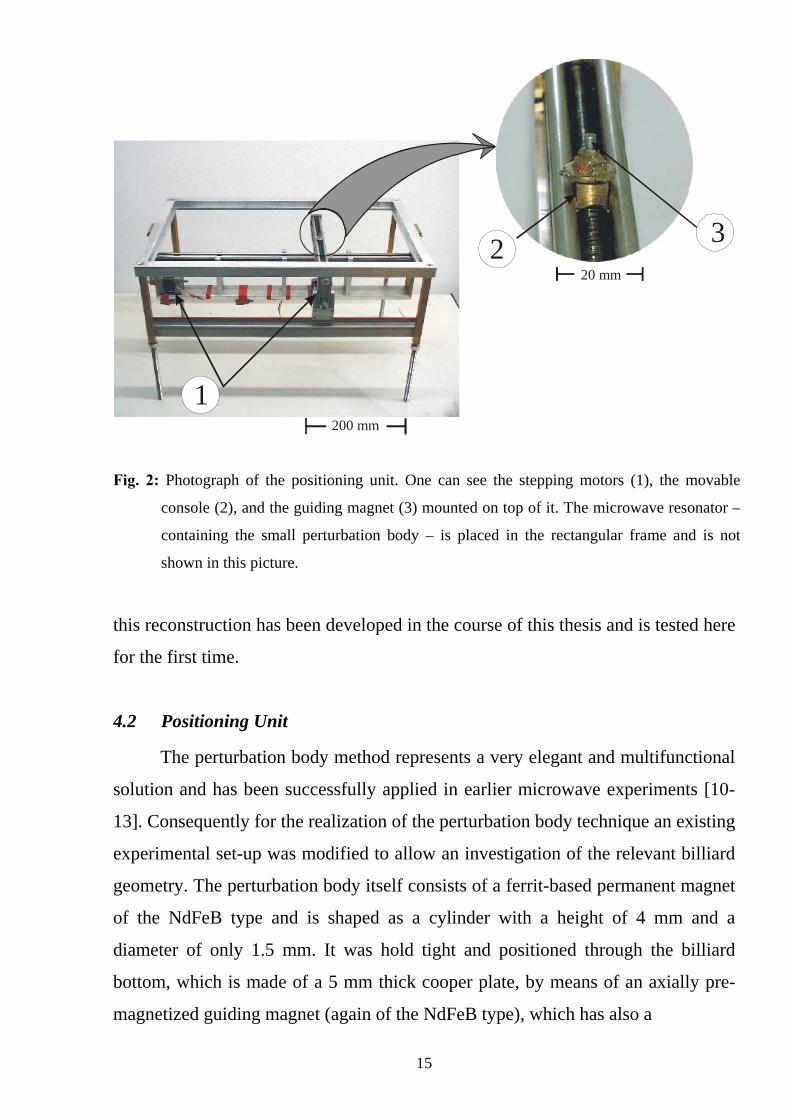
Fig. 2: Photograph of the positioning unit. One can see the stepping motors (1), the movable

console (2), and the guiding magnet (3) mounted on top of it. The microwave resonator –

containing the small perturbation body – is placed in the rectangular frame and is not

shown in this picture.

this reconstruction has been developed in the course of this thesis and is tested here

for the first time.

4.2 Positioning Unit

The perturbation body method represents a very elegant and multifunctional

solution and has been successfully applied in earlier microwave experiments [10-

13]. Consequently for the realization of the perturbation body technique an existing

experimental set-up was modified to allow an investigation of the relevant billiard

geometry. The perturbation body itself consists of a ferrit-based permanent magnet

of the NdFeB type and is shaped as a cylinder with a height of 4 mm and a

diameter of only 1.5 mm. It was hold tight and positioned through the billiard

bottom, which is made of a 5 mm thick cooper plate, by means of an axially pre-

magnetized guiding magnet (again of the NdFeB type), which has also a

15

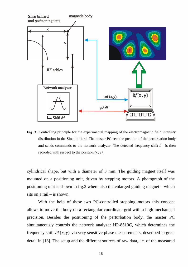
Fig. 3: Controlling principle for the experimental mapping of the electromagnetic field intensity

distribution in the Sinai billiard. The master PC sets the position of the perturbation body

and sends commands to the network analyzer. The detected frequency shift ∂f is then

recorded with respect to the position (x , y).

cylindrical shape, but with a diameter of 3 mm. The guiding magnet itself was

mounted on a positioning unit, driven by stepping motors. A photograph of the

positioning unit is shown in fig.2 where also the enlarged guiding magnet – which

sits on a rail – is shown.

With the help of these two PC-controlled stepping motors this concept

allows to move the body on a rectangular coordinate grid with a high mechanical

precision. Besides the positioning of the perturbation body, the master PC

simultaneously controls the network analyzer HP-8510C, which determines the

frequency shift ),( yxf∂ via very sensitive phase measurements, described in great

detail in [13]. The setup and the different sources of raw data, i.e. of the measured

16

frequency shifts f∂ and the positions (x,y) of the perturbation body inside the

resonator, are sketched in fig.3. According to (17) this finally yields the local

electromagnetic field intensity distribution, which is also exemplified in fig.4. The

intensity is commonly coded as ‘warmer’ colors, e.g. red or yellow, representing

high intensity areas and colors like blue representing areas with 02 ≈Er

.

According to the Mayer-Slater formula (17) the perturbation body method

only allows to investigate a combination of 2Er

and 2Br

inside the cavity.

Therefore the basic task is to adequately choose a perturbation body in such sense,

that on the one hand the body can be moved inside the resonator, while on the

other hand, mainly the electric component of the electromagnetic field intensity

should be affected, since only in this case the correspondence with the square of

the quantum wave function is given. The fact, that in the quasi-two-dimensional

resonator (with a transition frequency fcritical ≈ 30 GHz, which results from its

height of 5 mm) the electric field vector is oriented perpendicular to the billiard

plane, while the magnetic field vector lies parallel to this plane (TM mode), can be

used for an effective separation of both components of the electromagnetic field.

As described in [9], the interaction with a metallic body becomes optimal in the

case of an orientation along the lines of the field itself. Due to this, a metallic

cylinder with orientation perpendicular to the billiard’s surface was chosen. The

influence of the perturbation body size was studied in detail [11]. Therefore a

cylinder with a diameter of 1.5 mm and height 4 mm was used in the present

experiment. The maximum resolution which can be achieved in an experiment is

given by the diameter of the perturbation body and by the mechanics of the

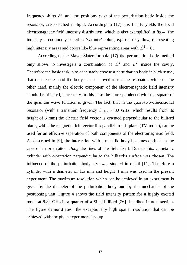
positioning unit. Figure 4 shows the field intensity pattern for a highly excited

mode at 8.82 GHz in a quarter of a Sinai billiard [26] described in next section.

The figure demonstrates the exceptionally high spatial resolution that can be

achieved with the given experimental setup.

17

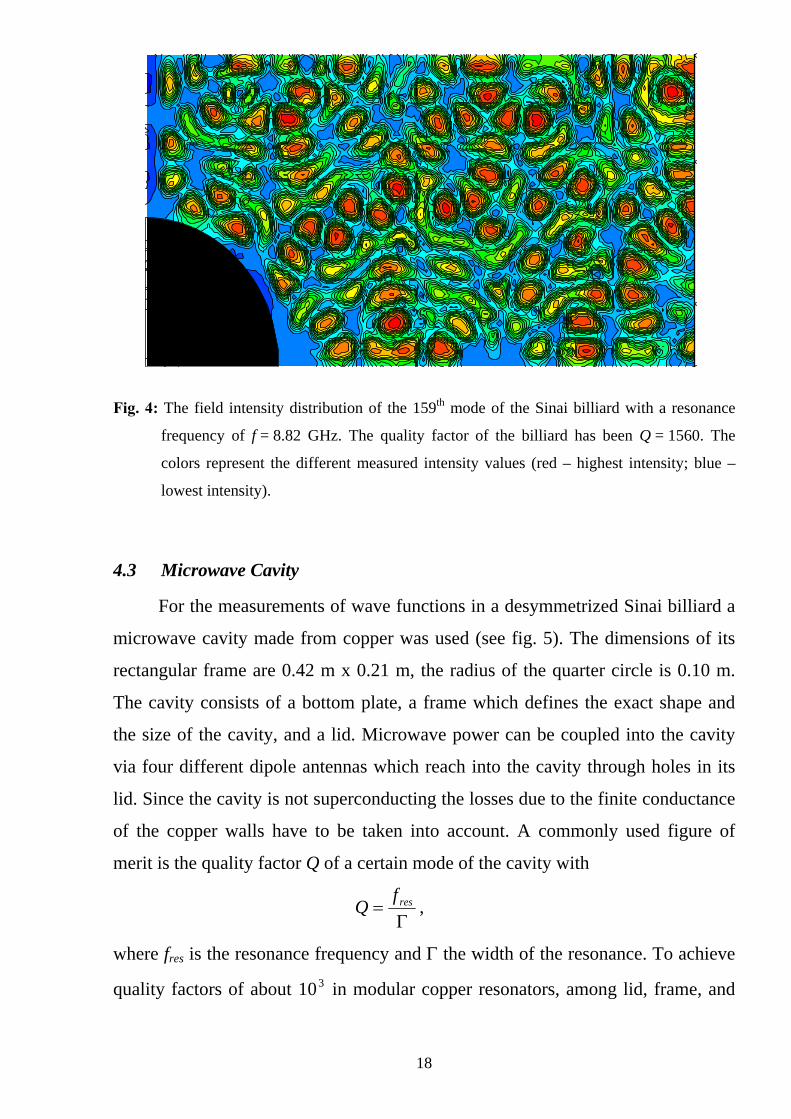
Fig. 4: The field intensity distribution of the 159th mode of the Sinai billiard with a resonance

frequency of f = 8.82 GHz. The quality factor of the billiard has been Q = 1560. The

colors represent the different measured intensity values (red – highest intensity; blue –

lowest intensity).

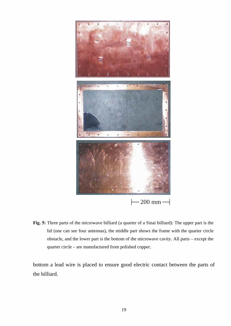
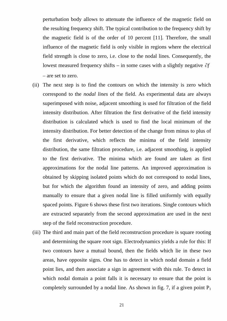
4.3 Microwave Cavity

For the measurements of wave functions in a desymmetrized Sinai billiard a

microwave cavity made from copper was used (see fig. 5). The dimensions of its

rectangular frame are 0.42 m x 0.21 m, the radius of the quarter circle is 0.10 m.

The cavity consists of a bottom plate, a frame which defines the exact shape and

the size of the cavity, and a lid. Microwave power can be coupled into the cavity

via four different dipole antennas which reach into the cavity through holes in its

lid. Since the cavity is not superconducting the losses due to the finite conductance

of the copper walls have to be taken into account. A commonly used figure of

merit is the quality factor Q of a certain mode of the cavity with

Γ

= resfQ ,

where fres is the resonance frequency and Γ the width of the resonance. To achieve

quality factors of about in modular copper resonators, among lid, frame, and 310

18

200 mm

Fig. 5: Three parts of the microwave billiard (a quarter of a Sinai billiard): The upper part is the

lid (one can see four antennas), the middle part shows the frame with the quarter circle

obstacle, and the lower part is the bottom of the microwave cavity. All parts – except the

quarter circle – are manufactured from polished copper.

bottom a lead wire is placed to ensure good electric contact between the parts of

the billiard.

19

5 Analysis and Results

In the following chapter the analysis of the field intensity distributions are

described. As mentioned above the first step in the analysis consists of a

reconstruction of the actual field distribution inside the cavity. The knowledge of

the nodal lines is necessary for this step that`s why an algorithm to find these lines

has been developed and is described in the following chapter. In further steps the

measured intensities are square rooted and signs are assigned – again with the help

of an algorithm. These field distributions form the basis for the calculation of the

correlation function of said eigenfunctions. A strong dependence on the states

number and an agreement between theory and experiment is observed. This is

expected since the theory presented in chapter 3 has been developed for the

semiclassical case and is discussed in chapter 5.3.

5.1 Field Reconstruction Procedure

As can be seen from (8) it is necessary to know the wave function, i.e. the

electric field in the microwave billiard, to obtain the autocorrelation function, but

the present experimental technique allows to measure electromagnetic field

intensities only. It is a principal difficulty, because one needs to find the sign of a

square root. In the general case this task has no solution and has to be solved in

each case individually. Therefore, a special field reconstruction procedure was

developed in the course of this thesis. For the first time in Darmstadt it allowed a

successful reconstruction of the distribution of the electric field from the measured

intensity distribution

The procedure consist of three steps which require the usage of computer

algorithms to cope with the large amount of data:

(i) In the experiment the shift of the resonant frequency is measured, which is a

combination of electric and magnetic field intensities. As one can see from the

Maier-Slater formula (17), the frequency shift can be negative or positive. As

described in chapter 4, an optimal choice of the size and the shape of the

20

perturbation body allows to attenuate the influence of the magnetic field on

the resulting frequency shift. The typical contribution to the frequency shift by

the magnetic field is of the order of 10 percent [11]. Therefore, the small

influence of the magnetic field is only visible in regions where the electrical

field strength is close to zero, i.e. close to the nodal lines. Consequently, the

lowest measured frequency shifts – in some cases with a slightly negative f∂

– are set to zero.

(ii) The next step is to find the contours on which the intensity is zero which

correspond to the nodal lines of the field. As experimental data are always

superimposed with noise, adjacent smoothing is used for filtration of the field

intensity distribution. After filtration the first derivative of the field intensity

distribution is calculated which is used to find the local minimum of the

intensity distribution. For better detection of the change from minus to plus of

the first derivative, which reflects the minima of the field intensity

distribution, the same filtration procedure, i.e. adjacent smoothing, is applied

to the first derivative. The minima which are found are taken as first

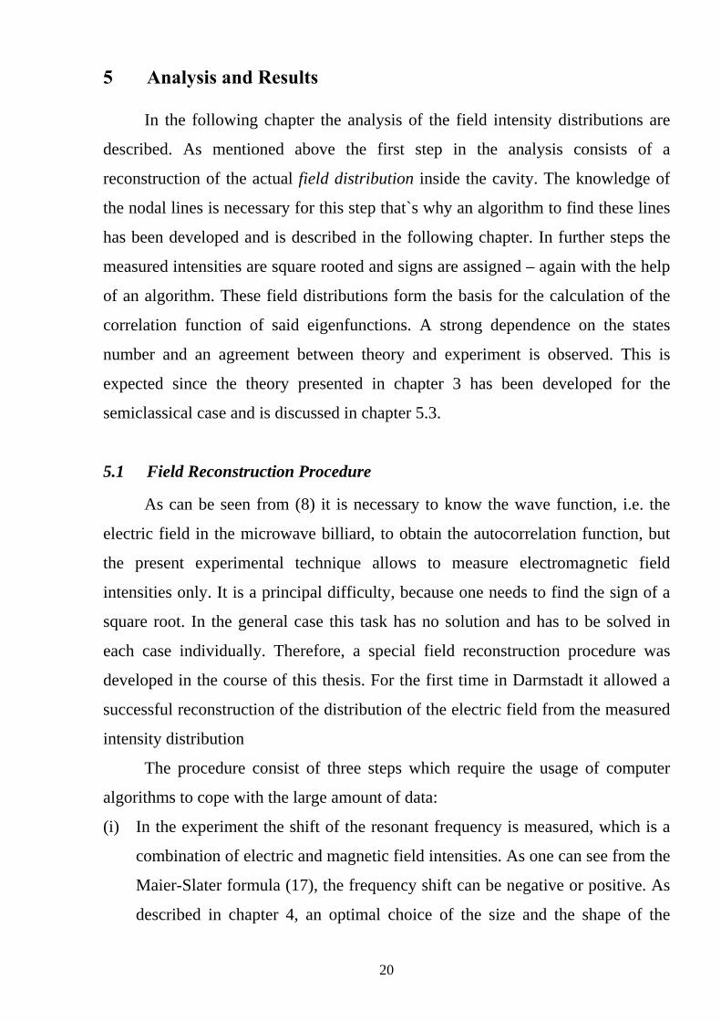
approximations for the nodal line patterns. An improved approximation is

obtained by skipping isolated points which do not correspond to nodal lines,

but for which the algorithm found an intensity of zero, and adding points

manually to ensure that a given nodal line is filled uniformly with equally

spaced points. Figure 6 shows these first two iterations. Single contours which

are extracted separately from the second approximation are used in the next

step of the field reconstruction procedure.

(iii) The third and main part of the field reconstruction procedure is square rooting

and determining the square root sign. Electrodynamics yields a rule for this: If

two contours have a mutual bound, then the fields which lie in these two

areas, have opposite signs. One has to detect in which nodal domain a field

point lies, and then associate a sign in agreement with this rule. To detect in

which nodal domain a point falls it is necessary to ensure that the point is

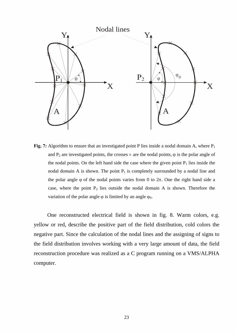
completely surrounded by a nodal line. As shown in fig. 7, if a given point P1

21

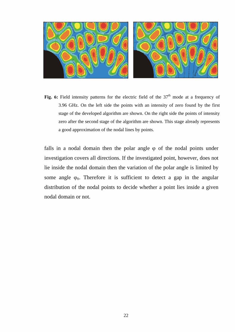
Fig. 6: Field intensity patterns for the electric field of the 37th mode at a frequency of

3.96 GHz. On the left side the points with an intensity of zero found by the first

stage of the developed algorithm are shown. On the right side the points of intensity

zero after the second stage of the algorithm are shown. This stage already represents

a good approximation of the nodal lines by points.

falls in a nodal domain then the polar angle ϕ of the nodal points under

investigation covers all directions. If the investigated point, however, does not

lie inside the nodal domain then the variation of the polar angle is limited by

some angle ϕ0. Therefore it is sufficient to detect a gap in the angular

distribution of the nodal points to decide whether a point lies inside a given

nodal domain or not.

22

A

Nodal lines

ϕ

Xϕ

ϕ 0

Y

A

X

Y

Fig. 7: Algorithm to ensure that an investigated point P lies inside a nodal domain A, where P1

and P2 are investigated points, the crosses × are the nodal points, ϕ is the polar angle of

the nodal points. On the left hand side the case where the given point P1 lies inside the

nodal domain A is shown. The point P1 is completely surrounded by a nodal line and

the polar angle ϕ of the nodal points varies from 0 to 2π. One the right hand side a

case, where the point P2 lies outside the nodal domain A is shown. Therefore the

variation of the polar angle ϕ is limited by an angle ϕ0.

One reconstructed electrical field is shown in fig. 8. Warm colors, e.g.

yellow or red, describe the positive part of the field distribution, cold colors the

negative part. Since the calculation of the nodal lines and the assigning of signs to

the field distribution involves working with a very large amount of data, the field

reconstruction procedure was realized as a C program running on a VMS/ALPHA

computer.

23

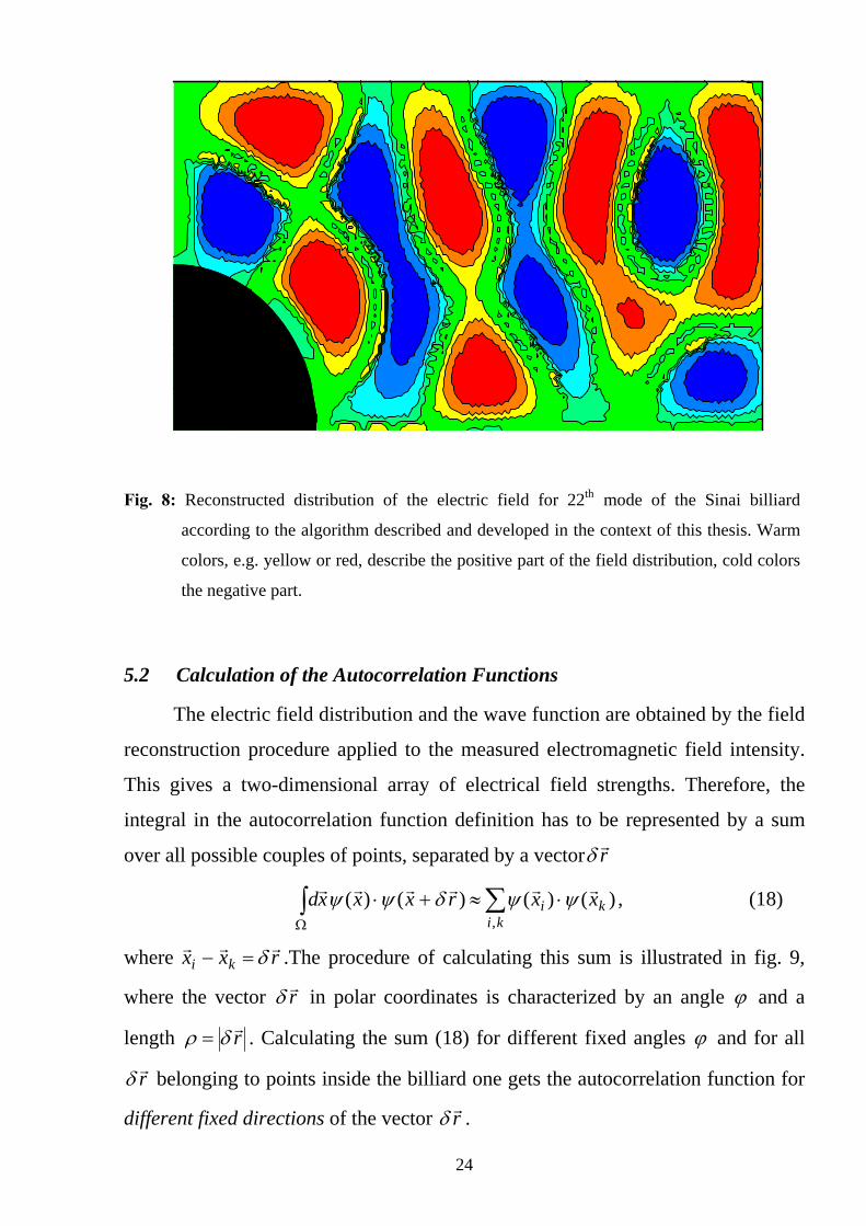
Fig. 8: Reconstructed distribution of the electric field for 22th mode of the Sinai billiard

according to the algorithm described and developed in the context of this thesis. Warm

colors, e.g. yellow or red, describe the positive part of the field distribution, cold colors

the negative part.

5.2 Calculation of the Autocorrelation Functions

The electric field distribution and the wave function are obtained by the field

reconstruction procedure applied to the measured electromagnetic field intensity.

This gives a two-dimensional array of electrical field strengths. Therefore, the

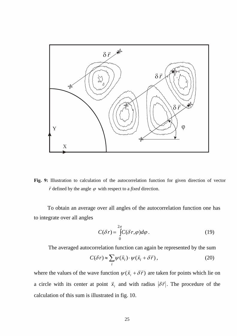
integral in the autocorrelation function definition has to be represented by a sum

over all possible couples of points, separated by a vector rrδ

∑∫ ⋅≈+⋅Ω ki

ki xxrxxxd,

)()()()( rrrrrr ψψδψψ , (18)

where rxx kirrr δ=− .The procedure of calculating this sum is illustrated in fig. 9,

where the vector rrδ in polar coordinates is characterized by an angle ϕ and a

length rrδρ = . Calculating the sum (18) for different fixed angles ϕ and for all

rrδ belonging to points inside the billiard one gets the autocorrelation function for

different fixed directions of the vector rrδ .

24

r

Y

r

r

ϕ

Fig. 9: Illustration to calculation of the autocorrelation function for given direction of vector

To obtain an average over all angles of the autocorrelation function one has

to integrate over all angles

∫=π

ϕϕδδ2

0),()( drCrC . (19)

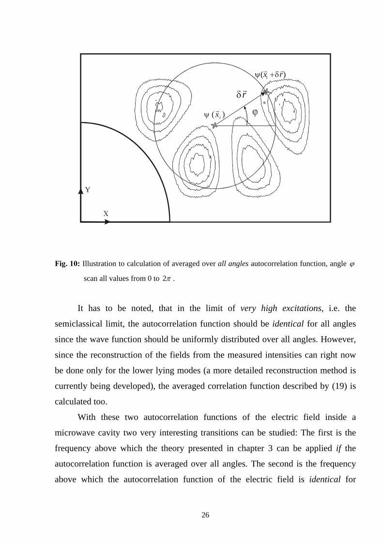
The averaged autocorrelation function can again be represented by the sum

∑ +⋅≈i

ii rxxrC )()()( rrr δψψδ , (20)

where the values of the wave function )( rxirr δψ + are taken for points which lie on

a circle with its center at point ixr and with radius rrδ . The procedure of the

calculation of this sum is illustrated in fig. 10.

rr defined by the angle ϕ with respect to a fixed direction.

25

Y

)( rxi δψ +

)( ixψ

r

ϕ

Fig. 10: Illustration to calculation of averaged over all angles autocorrelation function, angle ϕ

scan all values from 0 to π2 .

It has to be noted, that in the limit of very high excitations, i.e. the

semiclassical limit, the autocorrelation function should be identical for all angles

since the wave function should be uniformly distributed over all angles. However,

since the reconstruction of the fields from the measured intensities can right now

be done only for the lower lying modes (a more detailed reconstruction method is

currently being developed), the averaged correlation function described by (19) is

calculated too.

With these two autocorrelation functions of the electric field inside a

microwave cavity two very interesting transitions can be studied: The first is the

frequency above which the theory presented in chapter 3 can be applied if the

autocorrelation function is averaged over all angles. The second is the frequency

above which the autocorrelation function of the electric field is identical for

26

different angles, i.e. the range above which all directional information is lost. The

latter is commonly called the road to ergodicity.

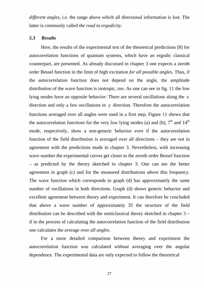
5.3 Results

Here, the results of the experimental test of the theoretical predictions [8] for

autocorrelation functions of quantum systems, which have an ergodic classical

counterpart, are presented. As already discussed in chapter 3 one expects a zeroth

order Bessel function in the limit of high excitation for all possible angles. Thus, if

the autocorrelation function does not depend on the angle, the amplitude

distribution of the wave function is isotropic, too. As one can see in fig. 11 the low

lying modes have an opposite behavior: There are several oscillations along the x

direction and only a few oscillations in direction. Therefore the autocorrelation

functions averaged over all angles were used in a first step. Figure

y

11 shows that

the autocorrelation functions for the very low lying modes (a) and (b), 7th and 14th

mode, respectively, show a non-generic behavior even if the autocorrelation

function of the field distribution is averaged over all directions – they are not in

agreement with the predictions made in chapter 3. Nevertheless, with increasing

wave number the experimental curves get closer to the zeroth order Bessel function

– as predicted by the theory sketched in chapter 3. One can see the better

agreement in graph (c) and for the measured distributions above this frequency.

The wave function which corresponds to graph (d) has approximately the same

number of oscillations in both directions. Graph (d) shows generic behavior and

excellent agreement between theory and experiment. It can therefore be concluded

that above a wave number of approximately 35 the structure of the field

distribution can be described with the semiclassical theory sketched in chapter 3 –

if in the process of calculating the autocorrelation function of the field distribution

one calculates the average over all angles.

For a more detailed comparison between theory and experiment the

autocorrelation function was calculated without averaging over the angular

dependence. The experimental data are only expected to follow the theoretical

27

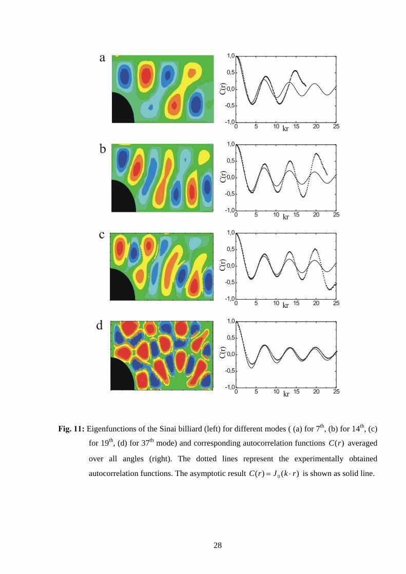
Fig. 11: Eigenfunctions of the Sinai billiard (left) for different modes ( (a) for 7th, (b) for 14th, (c)

for 19th, (d) for 37th mode) and corresponding autocorrelation functions averaged

over all angles (right). The dotted lines represent the experimentally obtained

autocorrelation functions. The asymptotic result

)(rC

)()( 0 rkJrC ⋅= is shown as solid line.

28

predictions if the field inside the cavity is distributed uniformly, i.e. all information

about the geometry of the boundary is lost for regions sufficiently far away from

the boundary. Figure 12 shows the autocorrelation functions for three different

angles.

The non-generic behavior of the autocorrelation functions in fig.12 (a), (b)

and (c) for different angles 2

,4

,0 ππϕ = is expected, because the wave

functions – as one can see from the corresponding picture – show different

numbers of oscillations for different directions. Even the autocorrelation functions

which are shown in fig.12 (d) do not show the expected behavior despite the fact

that the number of oscillations along the x and y direction are nearly the same.

Here the height of the oscillations is of the correct magnitude but their ‘frequency’

is not in accordance with theory.

There might be several reasons for these remaining discrepancies. On the

one hand one might still be at frequencies for which the field is not distributed

uniformly. On the other hand similar facts were found by other authors which have

numerically studied ergodic billiards [18,19] even at higher energies. In other

words these results seem to indicate that the Wigner functions exhibit more

structure on the energetic surface than does the Liouville density for an ergodic

theory and show non ergodic features. At present it is unclear whether these

differences spring from the fact that only modes in the low and medium frequency

regime are investigated or whether these non-generic properties are related to

special features of the Sinai billiard like the so-called bouncing ball orbits.

29

Fig. 12: Eigenfunctions of the Sinai billiard (left) for different modes ((a) for 14th, (b) for 19th,

(c) for 21th, (d) for 37th mode) and corresponding autocorrelation functions obtained for

three different angles (right). Red curves show experimentally obtained autocorrelation

functions for 0=ϕ , blue one for 4πϕ = , green one for

2πϕ = . Black curves show

zeroth order Bessel functions.

30

6 Conclusion and Outlook

For the investigation of autocorrelation function properties of ergodic

systems a field reconstruction procedure was developed. This procedure allows to

half-automatically deduce the field from the experimentally measured

electromagnetic field intensity. For the calculation of the spatial autocorrelation

function two further procedures were developed, one for the calculation of the

averaged autocorrelation function and one for the calculation of the angular

dependence of the autocorrelation function. An autocorrelation function averaged

over all angles demonstrated good agreement with theory. It has also been

interesting to investigate the behavior of not averaged autocorrelation functions.

The results of this work show, however that for a more detailed investigation of

this quantity it is necessary go up to high excited states in the billiard. The

implementation of a field reconstruction procedure to high lying modes requires a

further improvement of this algorithm.

Another direction of further implementation of a field reconstruction

procedure is the investigation of the nodal domain distribution. Recent

investigations [25] show a direct connection between the nodal domain distribution

of the chaotic eigenfunction and the percolation theory.

31

References

[1] M.V. Berry, Eur. J. Phys. 2, 91 (1981).

[2] H.G. Schuster, Deterministic Chaos (VCH, Weinheim,1989).

[3] M.C. Gutzwiller, Chaos in Classical and Quantum Mechanics (Springer,

New York, 1990).

[4] M.C. Gutzwiller, J. Math. Phys. 12, 343 (1971)

[5] O. Bohigas, M. J. Giannoni, and C. Schmit, Phys. Rev. Lett. 52,1 (1984).

[6] H.-J. Stöckmann and J. Stein, Phys. Rev. Lett. 64, 2215 (1990).

[7] H.-D. Gräf, H. L. Harney, H. Lengeler, C. H. Lewenkopf, C. Rangacharyulu,

A. Richter, P. Schardt, and H. A. Weidenmüller, Phys. Rev. Lett. 69, 1296

(1992).

[8] M.V. Berry, J. Phys. A 10, 2083 (1977).

[9] L.C. Maier, Jr and J.C. Slater, J. Appl. Phys. 23, 1352 (1968).

[10] S. Sridhar, D.O. Hogenboom, and B. A. Willemsen, J. Stat. Phys. 68, 239

(1992).

[11] A. Gokirmark, D.H. Wu, J.S.A. Bridgewater, S.M. Anlage, Rev. Sci.

Instrum. 69, 3410 (1998).

[12] D.H. Wu, J.S.A. Bridgewater, A. Gokirmak, and S.M. Anlage, Phys. Rev.

Lett. 81, 2890 (1998).

[13] C. Dembowski, Diploma thesis (1997), TH Darmstadt, unpublished.

[14] L.A. Bunimovich, Funct. Anal. Appl. 8, 254 (1974).

[15] A. Messiah, Quantenmechanik Band 1 (de Gruyter, Berlin 1981).

[16] M.V. Berry, Proc. R. Soc. London A 413, 183 (1987).

[17] A. Richter, Playing Billiards with Microwaves - Quantum Manifestations of

Classical Chaos, in Emerging Applications of Number Theory, The IMA

Volumes in Mathematics and its Applications, Vol. 109, edited by D. A.

Hejhal, J. Friedman, M. C. Gutzwiller, and A. M. Odlyzko, pp. 479

(Springer, New York, 1999).

[18] M. Srednicki and F. Stiernelof, J. Phys. A 29, 5817 (1996).

32

[19] S.W. McDonald and A.N. Kaufman, Phys. Rev. A 37, 3067 (1988).

[20] V.I. Arnold, Mathematical Methods of Classical Mechanics (Springer-

Verlag, New-York,1978)

[21] V.P. Maslov and M.V. Fedoriuk, Semi-Classical Approximation in Quantum

Mechanics (Reidel, Dordrecht, 1981)

[22] E. Wigner, Phys. Rev. 40 749 (1932).

[23] M.V. Berry, Phil. Trans. R. Soc. A 287 237 (1977)

[24] A. Voros, in: Stochastic Behaviour in Classical and Quantum Hamiltonian

System, eds., G. Casati, J. Ford, Lecture notes in Physics 93 (Springer,

Berlin, 1979) 326.

[25] E. Bogomolny and C. Schmidt, nlin. CD/0110019 (2001), preprint.

[26] Y.G. Sinai,. Sov. Math. Dokl. 4, 1818 (1963).

33

34

Acknowledgements I would like to sincerely thank Professor Dr. Dr. h.c. mult. Achim Richter for

giving me the great opportunity to investgate such an exciting branch as quantum

chaos and for offering me the possibility to work in a modern laboratory.

Further I want thank Dr. Harald Genz for his care, support and valuable

advices.

Without the priceless help of Dr. Barbara Dietz-Pilatus, Dipl.- and Dipl.-

Phys. Christian Dembowski Phys. Andreas Heine this work would not be

imaginable. Thank you for the support, numerous discussions and advice which

has invaluable.

I would like to express my gratitude to Dipl.-Phys. Sergey Khodyachykh for

the everyday support.

Furthermore, I want to address my sincere gratitude to the Dean of the

Department of Physics and Technology (Karazin National University Kharkiv),

Professor Dr. N.A. Asarenkov, and to Dr. V.A. Kobyakov for their help in the

choice of my future profession, Dr. A.F. Schus for his help in solving the

organizational problems. Also I want to thank all professors and senior lecturers of

the Department of Physics and Technology who have contributed to my education.

Mrs. Sabine Genz I would like thank for the time she investigated to improve

my English.

My special thank goes to the family Hartmann, their friendly attitude

towards me.

Finally, my heartfelt gratitude to my parents Valentina and Victor Miski-

Oglu for their thoughts, warm and care.