Embed Size (px)
Citation preview
ZIGGURAT – DATA MODEL & FILE FORMAT A proposal by (mostly) Stefan Evert and (minimally) Andrew Hardie. Version 1.0 (2015-‐08-‐08) Ziggurat is the database engine for CWB4. It consists of a data model, a file format that expresses this model, and a software library for creating and accessing data organized according to the this model. The Ziggurat library will licensed under LGPLv3 or a more permissive non-‐copyleft license compatible with (L)GPLv3 (such as the Apache 2.0 License, which the GNU project recommends). Note that the library will build on other packages with different licenses, notably Glib2 (LGPL) and PCRE (BSD).
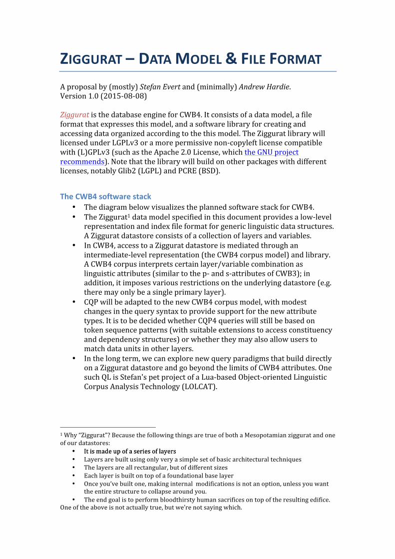
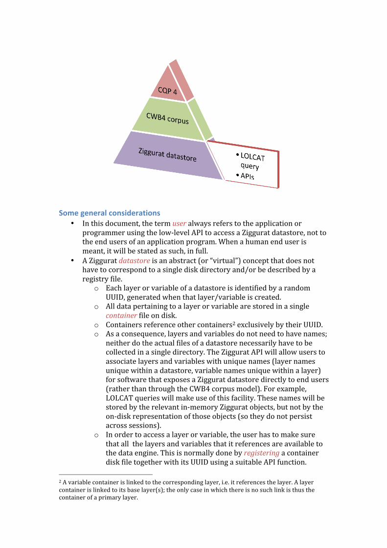
The CWB4 software stack • The diagram below visualizes the planned software stack for CWB4. • The Ziggurat1 data model specified in this document provides a low-‐level
representation and index file format for generic linguistic data structures. A Ziggurat datastore consists of a collection of layers and variables.
• In CWB4, access to a Ziggurat datastore is mediated through an intermediate-‐level representation (the CWB4 corpus model) and library. A CWB4 corpus interprets certain layer/variable combination as linguistic attributes (similar to the p-‐ and s-‐attributes of CWB3); in addition, it imposes various restrictions on the underlying datastore (e.g. there may only be a single primary layer).
• CQP will be adapted to the new CWB4 corpus model, with modest changes in the query syntax to provide support for the new attribute types. It is to be decided whether CQP4 queries will still be based on token sequence patterns (with suitable extensions to access constituency and dependency structures) or whether they may also allow users to match data units in other layers.
• In the long term, we can explore new query paradigms that build directly on a Ziggurat datastore and go beyond the limits of CWB4 attributes. One such QL is Stefan's pet project of a Lua-‐based Object-‐oriented Linguistic Corpus Analysis Technology (LOLCAT).
1 Why “Ziggurat”? Because the following things are true of both a Mesopotamian ziggurat and one of our datastores:
• It is made up of a series of layers • It is made up of a series of layers • Layers are built using only very a simple set of basic architectural techniques • The layers are all rectangular, but of different sizes • Each layer is built on top of a foundational base layer • Once you’ve built one, making internal modifications is not an option, unless you want
the entire structure to collapse around you. • The end goal is to perform bloodthirsty human sacrifices on top of the resulting edifice.
One of the above is not actually true, but we’re not saying which.
Some general considerations • In this document, the term user always refers to the application or
programmer using the low-‐level API to access a Ziggurat datastore, not to the end users of an application program. When a human end user is meant, it will be stated as such, in full.
• A Ziggurat datastore is an abstract (or “virtual”) concept that does not have to correspond to a single disk directory and/or be described by a registry file.
o Each layer or variable of a datastore is identified by a random UUID, generated when that layer/variable is created.
o All data pertaining to a layer or variable are stored in a single container file on disk.
o Containers reference other containers2 exclusively by their UUID. o As a consequence, layers and variables do not need to have names;
neither do the actual files of a datastore necessarily have to be collected in a single directory. The Ziggurat API will allow users to associate layers and variables with unique names (layer names unique within a datastore, variable names unique within a layer) for software that exposes a Ziggurat datastore directly to end users (rather than through the CWB4 corpus model). For example, LOLCAT queries will make use of this facility. These names will be stored by the relevant in-‐memory Ziggurat objects, but not by the on-‐disk representation of those objects (so they do not persist across sessions).
o In order to access a layer or variable, the user has to make sure that all the layers and variables that it references are available to the data engine. This is normally done by registering a container disk file together with its UUID using a suitable API function.
2 A variable container is linked to the corresponding layer, i.e. it references the layer. A layer container is linked to its base layer(s); the only case in which there is no such link is thus the container of a primary layer.
o As a consequence of this, the low-‐level data engine has no need for the concept of a datastore as a separate, fixed unit. In particular, container files can be spread across different disk directories, and new layers and variables can be registered at any time. Consistency is always ensured by the UUID-‐based references.
o Users are encouraged to think of a datastore as the set of layers and variables pertaining to a particular corpus. It is recommended to collect the corresponding container files in a single disk directory, and the API will offer convenience functions for registering all containers found in such a directory or listed in a text file with UUID/filename combinations.3
o This approach has two important advantages: (i) It is easy for end-‐users to add “private” annotations at runtime by registering the layers and variables corresponding to a new CWB4 attribute. No write access to a main index directory or registry file is required, and the new annotations will never affect other users. (ii) The UUID-‐based referencing scheme guarantees consistency of primary data and annotations. If primary data are changed (e.g. by re-‐encoding a corpus, or changing the sentence boundaries underlying an alignment attribute), a new UUID is assigned and references from other annotation layers become invalid (or can still be resolved to the old version of the corpus if the container files are archived and registered). Query results also embed UUIDs of the layers they are based on, so they can safely be stored on disk (whereas CQP3 saved queries reference the corpus by name and may be inconsistent if the corpus has been re-‐encoded in the meantime).
• The notion of a CWB4 corpus is defined in the intermediate-‐level corpus model. It is a collection of linguistic attributes, backed by a Ziggurat datastore. A corpus is more restricted than a datastore; for example:
o There must be exactly one primary layer in a corpus. o Attributes imply a particular linguistic interpretation of the
underlying Ziggurat data structures, e.g. an XML/constituency attribute treats the nodes of a tree layer as XML elements.
o Attributes build on a Ziggurat layer, but often require additional mandatory variables: e.g. an XML attribute requires an indexed string variable specifying element names, and a dependency attribute requires an indexed string variable specifying relation types.
o In addition, each CWB4 corpus will be described by a single metadata file, similar to a CWB3 registry file. This file will be stored in the same directory as the index files, however. Runtime extensions (e.g. with user attributes) should be allowed.
o CWB4 attributes should also be assigned random UUIDs to ensure referential integrity (esp. with private user attributes).
3 The use of such a registration file is more efficient because the individual file containers do not need to be opened until the respective layer or variable is accessed. For example, CQP 4 may need to register all available corpora in order to resolve references to the base layers of alignment attributes.
• Main design principle: KISS o For a tool that will be maintained and developed exclusively by a
small volunteer community, code simplicity is an essential requirement. It's better to have a simple tool that works and that is actively maintained than a complex and highly optimized software that only a single person understands (which is our first impression of BlackLab, for instance).
o In other words, we don't want CWB4 to become the Perl 6 of corpus query engines …
• Consequences of the KISS approach o Introduce as few different value types as possible; e.g., every
number is a signed 64-‐bit integer, even though lexicon IDs could be stored more compactly as 32-‐bit values.
o Don't use different encodings for the same value type; e.g. integers are always encoded as signed 64-‐bit values, even though an unsigned representation would allow slightly better compression if values are known to be non-‐negative.
o Rely on a small number of generic data structures (vector, set vector, sort index, inverted index; see definitions somewhere below) instead of defining customized data structures with faster lookup or better compression rates; e.g. prefer sort index with logarithmic lookup to constant-‐time hash lookup or B-‐trees with better memory/disk locality. Don't use a clustered sort index to speed up frequent operations by avoiding access to the underlying vector (e.g. when traversing a graph).
o Obvious potential for optimizations of moderate complexity (such as using B-‐trees instead of sort indexes) is highlighted in the draft specification and should perhaps be considered in a later phase once all basic work is complete.
This box describes potential for future optimization. o CQP 4 will use the same brute-‐force approach as CQP 3, relying on
fast corpus traversal with simple C code rather than clever use of sophisticated indexes. Note that we don't make great efforts to speed up common traversal steps (such as following a graph edge) with the help of complicated data structures either.
o In line with the KISS approach we will not attempt any multithread programming within Ziggurat. However, we will make the Ziggurat library compatible with multithread usage (no global variables or non-‐thread-‐specific buffers, for instance), that is, all Ziggurat functions will be re-‐entrant.
Ziggurat data model
Data model A Ziggurat datastore (which is an abstraction that can be interpreted by higher-‐level components of CWB4 as a corpus) is a collection of data layers. A data layer is an ordered sequence of data units, each of which has values for one or more variables. Each data unit in a layer is annotated with the same set of variables. It
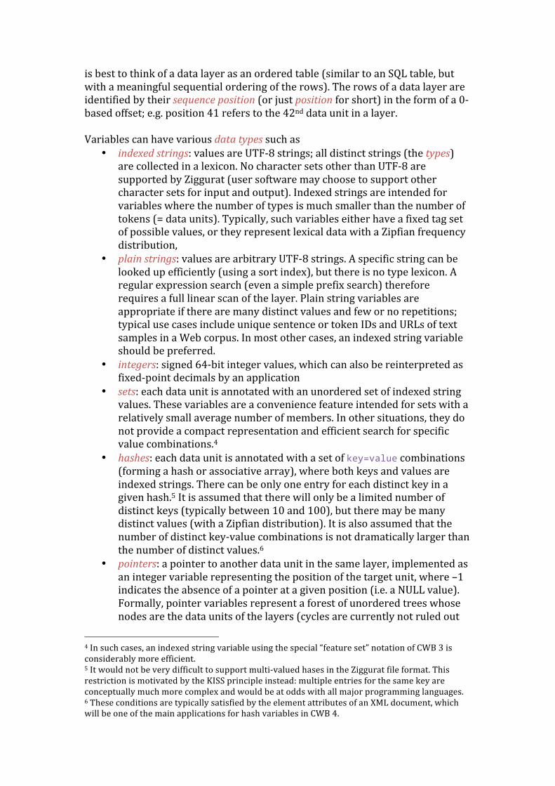
is best to think of a data layer as an ordered table (similar to an SQL table, but with a meaningful sequential ordering of the rows). The rows of a data layer are identified by their sequence position (or just position for short) in the form of a 0-‐based offset; e.g. position 41 refers to the 42nd data unit in a layer. Variables can have various data types such as
• indexed strings: values are UTF-‐8 strings; all distinct strings (the types) are collected in a lexicon. No character sets other than UTF-‐8 are supported by Ziggurat (user software may choose to support other character sets for input and output). Indexed strings are intended for variables where the number of types is much smaller than the number of tokens (= data units). Typically, such variables either have a fixed tag set of possible values, or they represent lexical data with a Zipfian frequency distribution,
• plain strings: values are arbitrary UTF-‐8 strings. A specific string can be looked up efficiently (using a sort index), but there is no type lexicon. A regular expression search (even a simple prefix search) therefore requires a full linear scan of the layer. Plain string variables are appropriate if there are many distinct values and few or no repetitions; typical use cases include unique sentence or token IDs and URLs of text samples in a Web corpus. In most other cases, an indexed string variable should be preferred.
• integers: signed 64-‐bit integer values, which can also be reinterpreted as fixed-‐point decimals by an application
• sets: each data unit is annotated with an unordered set of indexed string values. These variables are a convenience feature intended for sets with a relatively small average number of members. In other situations, they do not provide a compact representation and efficient search for specific value combinations.4
• hashes: each data unit is annotated with a set of key=value combinations (forming a hash or associative array), where both keys and values are indexed strings. There can be only one entry for each distinct key in a given hash.5 It is assumed that there will only be a limited number of distinct keys (typically between 10 and 100), but there may be many distinct values (with a Zipfian distribution). It is also assumed that the number of distinct key-‐value combinations is not dramatically larger than the number of distinct values.6
• pointers: a pointer to another data unit in the same layer, implemented as an integer variable representing the position of the target unit, where –1 indicates the absence of a pointer at a given position (i.e. a NULL value). Formally, pointer variables represent a forest of unordered trees whose nodes are the data units of the layers (cycles are currently not ruled out
4 In such cases, an indexed string variable using the special “feature set” notation of CWB 3 is considerably more efficient. 5 It would not be very difficult to support multi-‐valued hases in the Ziggurat file format. This restriction is motivated by the KISS principle instead: multiple entries for the same key are conceptually much more complex and would be at odds with all major programming languages. 6 These conditions are typically satisfied by the element attributes of an XML document, which will be one of the main applications for hash variables in CWB 4.
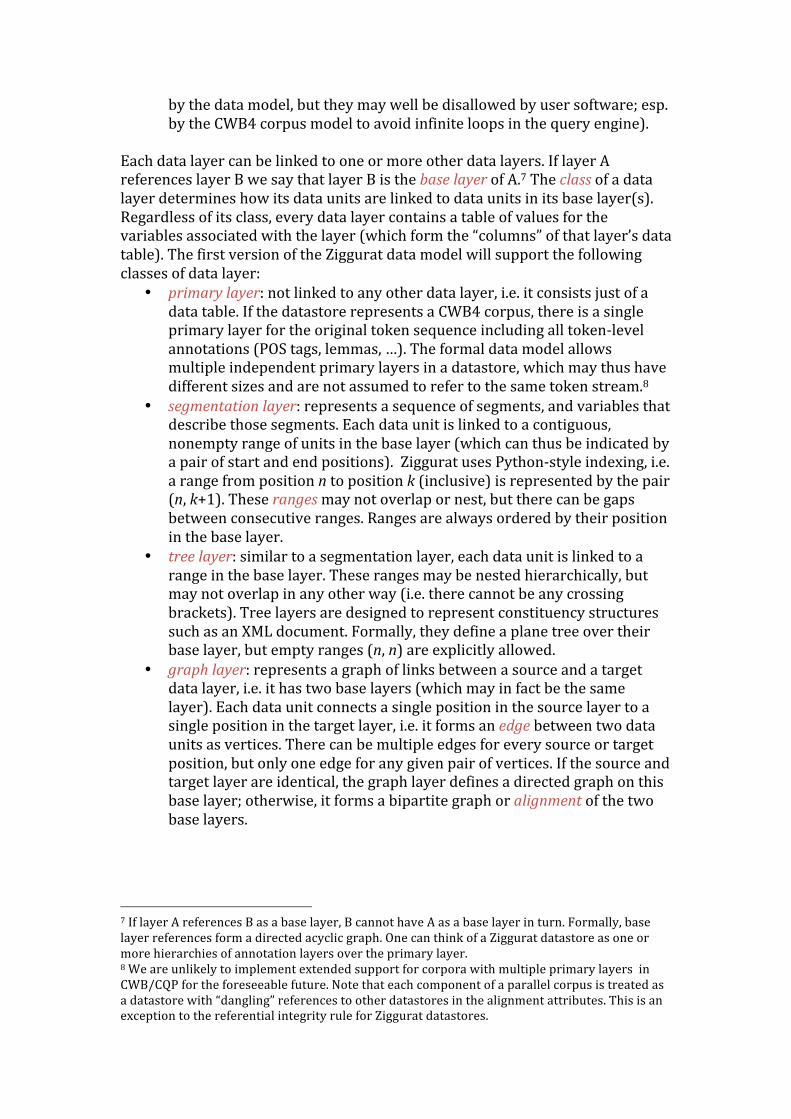
by the data model, but they may well be disallowed by user software; esp. by the CWB4 corpus model to avoid infinite loops in the query engine).
Each data layer can be linked to one or more other data layers. If layer A references layer B we say that layer B is the base layer of A.7 The class of a data layer determines how its data units are linked to data units in its base layer(s). Regardless of its class, every data layer contains a table of values for the variables associated with the layer (which form the “columns” of that layer’s data table). The first version of the Ziggurat data model will support the following classes of data layer:
• primary layer: not linked to any other data layer, i.e. it consists just of a data table. If the datastore represents a CWB4 corpus, there is a single primary layer for the original token sequence including all token-‐level annotations (POS tags, lemmas, …). The formal data model allows multiple independent primary layers in a datastore, which may thus have different sizes and are not assumed to refer to the same token stream.8
• segmentation layer: represents a sequence of segments, and variables that describe those segments. Each data unit is linked to a contiguous, nonempty range of units in the base layer (which can thus be indicated by a pair of start and end positions). Ziggurat uses Python-‐style indexing, i.e. a range from position n to position k (inclusive) is represented by the pair (n, k+1). These ranges may not overlap or nest, but there can be gaps between consecutive ranges. Ranges are always ordered by their position in the base layer.
• tree layer: similar to a segmentation layer, each data unit is linked to a range in the base layer. These ranges may be nested hierarchically, but may not overlap in any other way (i.e. there cannot be any crossing brackets). Tree layers are designed to represent constituency structures such as an XML document. Formally, they define a plane tree over their base layer, but empty ranges (n, n) are explicitly allowed.
• graph layer: represents a graph of links between a source and a target data layer, i.e. it has two base layers (which may in fact be the same layer). Each data unit connects a single position in the source layer to a single position in the target layer, i.e. it forms an edge between two data units as vertices. There can be multiple edges for every source or target position, but only one edge for any given pair of vertices. If the source and target layer are identical, the graph layer defines a directed graph on this base layer; otherwise, it forms a bipartite graph or alignment of the two base layers.
7 If layer A references B as a base layer, B cannot have A as a base layer in turn. Formally, base layer references form a directed acyclic graph. One can think of a Ziggurat datastore as one or more hierarchies of annotation layers over the primary layer. 8 We are unlikely to implement extended support for corpora with multiple primary layers in CWB/CQP for the foreseeable future. Note that each component of a parallel corpus is treated as a datastore with “dangling” references to other datastores in the alignment attributes. This is an exception to the referential integrity rule for Ziggurat datastores.
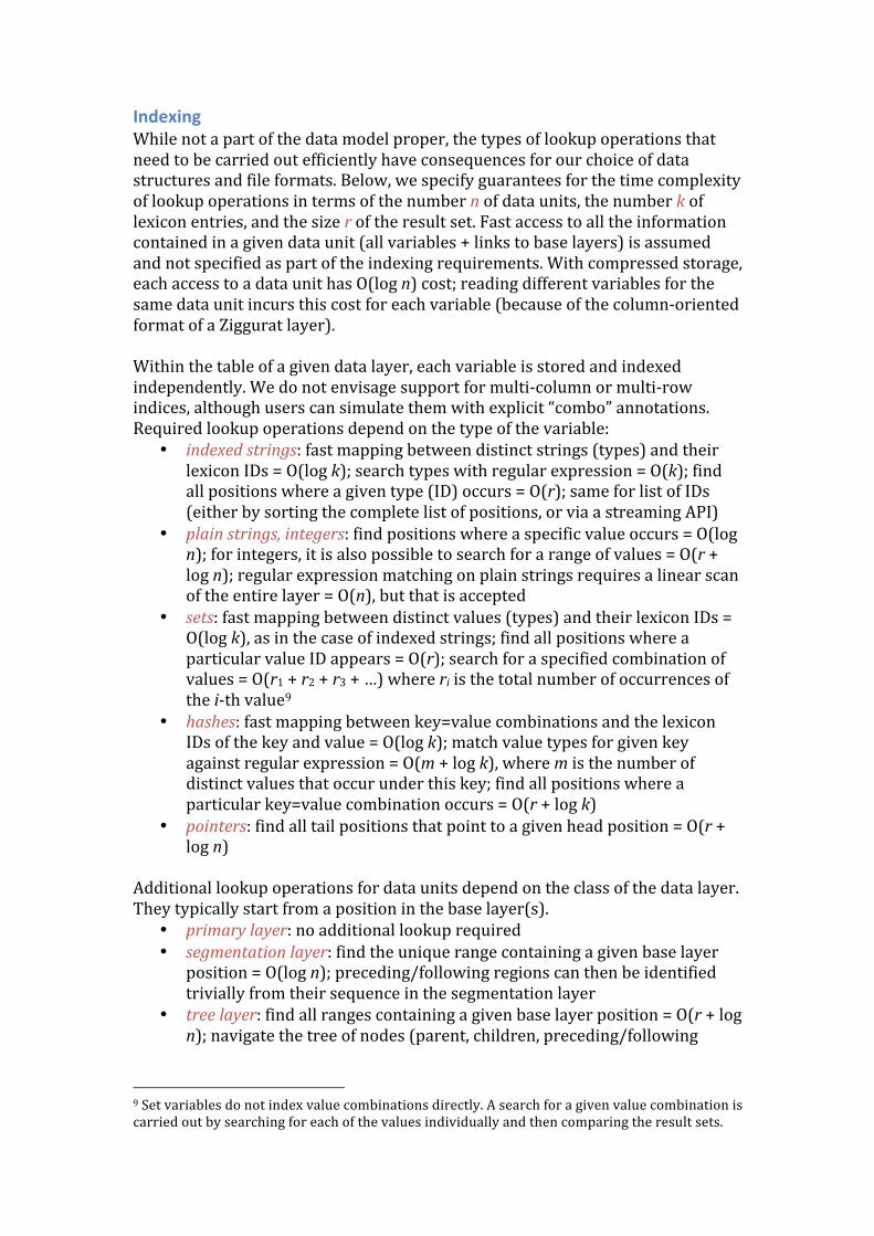
Indexing While not a part of the data model proper, the types of lookup operations that need to be carried out efficiently have consequences for our choice of data structures and file formats. Below, we specify guarantees for the time complexity of lookup operations in terms of the number n of data units, the number k of lexicon entries, and the size r of the result set. Fast access to all the information contained in a given data unit (all variables + links to base layers) is assumed and not specified as part of the indexing requirements. With compressed storage, each access to a data unit has O(log n) cost; reading different variables for the same data unit incurs this cost for each variable (because of the column-‐oriented format of a Ziggurat layer). Within the table of a given data layer, each variable is stored and indexed independently. We do not envisage support for multi-‐column or multi-‐row indices, although users can simulate them with explicit “combo” annotations. Required lookup operations depend on the type of the variable:
• indexed strings: fast mapping between distinct strings (types) and their lexicon IDs = O(log k); search types with regular expression = O(k); find all positions where a given type (ID) occurs = O(r); same for list of IDs (either by sorting the complete list of positions, or via a streaming API)
• plain strings, integers: find positions where a specific value occurs = O(log n); for integers, it is also possible to search for a range of values = O(r + log n); regular expression matching on plain strings requires a linear scan of the entire layer = O(n), but that is accepted
• sets: fast mapping between distinct values (types) and their lexicon IDs = O(log k), as in the case of indexed strings; find all positions where a particular value ID appears = O(r); search for a specified combination of values = O(r1 + r2 + r3 + …) where ri is the total number of occurrences of the i-‐th value9
• hashes: fast mapping between key=value combinations and the lexicon IDs of the key and value = O(log k); match value types for given key against regular expression = O(m + log k), where m is the number of distinct values that occur under this key; find all positions where a particular key=value combination occurs = O(r + log k)
• pointers: find all tail positions that point to a given head position = O(r + log n)
Additional lookup operations for data units depend on the class of the data layer. They typically start from a position in the base layer(s).
• primary layer: no additional lookup required • segmentation layer: find the unique range containing a given base layer
position = O(log n); preceding/following regions can then be identified trivially from their sequence in the segmentation layer
• tree layer: find all ranges containing a given base layer position = O(r + log n); navigate the tree of nodes (parent, children, preceding/following
9 Set variables do not index value combinations directly. A search for a given value combination is carried out by searching for each of the values individually and then comparing the result sets.
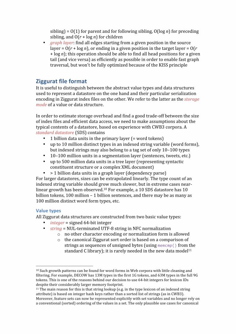
sibling) = O(1) for parent and for following sibling, O(log n) for preceding sibling, and O(r + log n) for children
• graph layer: find all edges starting from a given position in the source layer = O(r + log n), or ending in a given position in the target layer = O(r + log n); this operation should be able to find all head positions for a given tail (and vice versa) as efficiently as possible in order to enable fast graph traversal, but won't be fully optimized because of the KISS principle
Ziggurat file format It is useful to distinguish between the abstract value types and data structures used to represent a datastore on the one hand and their particular serialization encoding in Ziggurat index files on the other. We refer to the latter as the storage mode of a value or data structure. In order to estimate storage overhead and find a good trade-‐off between the size of index files and efficient data access, we need to make assumptions about the typical contents of a datastore, based on experience with CWB3 corpora. A standard datastore (SDS) contains
• 1 billion data units in the primary layer (= word tokens) • up to 10 million distinct types in an indexed string variable (word forms),
but indexed strings may also belong to a tag set of only 10–100 types • 10–100 million units in a segmentation layer (sentences, tweets, etc.) • up to 500 million data units in a tree layer (representing syntactic
constituent structure or a complex XML document) • > 1 billion data units in a graph layer (dependency parse)
For larger datastores, sizes can be extrapolated linearly. The type count of an indexed string variable should grow much slower, but in extreme cases near-‐linear growth has been observed.10 For example, a 10 SDS datastore has 10 billion tokens, 100 million – 1 billion sentences, and there may be as many as 100 million distinct word form types, etc.
Value types All Ziggurat data structures are constructed from two basic value types:
• integer = signed 64-‐bit integer • string = NUL-‐terminated UTF-‐8 string in NFC normalization
o no other character encoding or normalization form is allowed o the canonical Ziggurat sort order is based on a comparison of
strings as sequences of unsigned bytes (using memcmp() from the standard C library); it is rarely needed in the new data model11
10 Such growth patterns can be found for word forms in Web corpora with little cleaning and filtering. For example, DECOW has 13M types in the first 1G tokens, and 63M types in the full 9G tokens. This is one of the reasons behind our decision to use 64-‐bit integers for lexicon IDs despite their considerably larger memory footprint. 11 The main reason for this is that string lookup (e.g. in the type lexicon of an indexed string attribute) is based on integer hash keys rather than a sorted list of strings (as in CWB3). Moreover, feature sets can now be represented explicitly with set variables and no longer rely on a conventional (sorted) ordering of the values in a set. The only plausible use cases for canonical
o the canonical hashing algorithm for strings is a modified 64-‐bit version of the hash function used in CWB 3.5, which is itself a modification of DJB2a; the precise details of the algorithm are to be specified
Other hash functions should be explored based on experiments with realistic data sets in order to measure speed of computation and uniform distribution of the hash values.12 Following the KISS principle, we should stick with a simple algorithm that processes one byte at a time unless there are very good reasons to use a more complex method.
The low-‐level datastore API and implementation should only use variables of these two types (as well as structures and vectors composed from such variables), with few exceptions (e.g. bit vectors could be used as an in-‐memory representation for a set of lexicon IDs matching/not matching a given regular expression, as the CWB3 does). Storage modes for basic value types:
• Int: signed 64-‐bit integer in little-‐endian byte order13; must be aligned on an 8-‐byte boundary within the disk file
• VarInt: variable-‐length encoding of a signed 64-‐bit integer, using a modified version of the SQLite varint format. This modification is as follows: If the 2nd bit of the first byte is set, the binary complement of the encoded value is computed, so that small negative values also have a compact encoding (in the original format, negative values always require 9 bytes of storage).14 A VarInt is between 1 and 9 bytes long; it does not have to start on a particular boundary.15
• String: NUL-‐terminated UTF-‐8 string in NFC normalization. Consecutive strings can be packed without padding since no alignment is required.
sorting in Ziggurat are out-‐of-‐core (i.e. on-‐disk) merge sorts and the combination of data tables from different sources. 12 See http://programmers.stackexchange.com/questions/49550/which-‐hashing-‐algorithm-‐is-‐best-‐for-‐uniqueness-‐and-‐speed for a list of hash functions with benchmarks & collision counts. 13 This is intended to reduce overhead from endianness conversion, since the dominant CPU architecture for the forseeable future (x86_64) uses a little-‐endian byte order. It clashes with the widespread use of big-‐endian byte order for platform-‐independent file formats (in particular IP, hence also known as “network order”) and means that the (presumably efficient) POSIX macros nothl() and htonl() cannot be used for the conversion. The low-‐level API will need to define its own conversion macros, which are no-‐ops on little-‐endian platforms. Note that gcc has intrinsic macros __builtin_bswap32 and __builtin_bswap64, which are efficient on major CPUs. 14 In particular, values between –64 and +63 can be encoded in a single byte, values between –8192 and +8191 in two bytes, and values between –1048576 and +1048575 in three bytes. 15 If integer values are known to be non-‐negative – typical examples are lexicon IDs or an increasing sequence with δ-‐compression – it would be slightly more size-‐efficient to use the original SQLite varint format without a sign bit (which we call the UVarInt storage mode). A UVarInt can store values up to +127 in a single byte, and up to +16383 in two bytes, but would require 9 bytes to encode any negative value. Mixed use of VarInt and UVarInt storage modes seems error-‐prone (because the same bit patterns are valid in both modes but encode different numbers), and we decided that the additional overhead is justified by the easier implementation. See also the note in the introduction about the KISS principle!
Generic data structures All layers and variables in a Ziggurat datastore are constructed from only five generic data structures:
• a blob of arbitrary binary data (usually unpadded Strings); • a vector of fixed-‐sized elements (i.e. tuples of integers); • a vector of variable-‐length items (i.e. lists of integers); • a sort index with integer sort keys; and • an. inverse index, which enumerates the occurrences of each one of a set
of types. In this section, we describe the abstract data structures at a conceptual level, work out storage modes for their serialization in index files, and list the main access patterns afforded by the data structures. In the following section, the components making up different layer and variable types are defined in terms of the generic data structures. Most data structures offer an uncompressed and a compressed storage mode. For each layer/variable component the specification mandates either compressed or uncompressed storage, depending on the expected data size and access patterns. The general recommendation is to use uncompressed storage for O(k) data size (i.e. data structures over types), and compressed storage for O(n) data size (i.e. data structures over tokens or annotation elements).
Additional, more specialized data structures might achieve better performance for certain access patterns, but have been rejected in favour of the KISS principle. We might want to reconsider this decision when a first implementation is available for benchmarks.
A blob is a block of arbitrary binary data that is interpreted by the application. Blobs are most commonly used to hold unpadded String values.
• The only supported access pattern is to read a specified number of bytes or a NUL-‐terminated string from a given offset in the blob.
A vector is a sequence of fixed-‐size items (i.e. integers or tuples of integers, which are the only fixed-‐size values in Ziggurat) accessed by their position in the sequence (enumerated starting from 0).
• The main access pattern is to read the item at a given position. Sequential reads of consecutive positions (either ascending or descending) should be particularly efficient.
• In uncompressed storage mode, a vector of length n over d-‐tuples of integers is serialized as a sequence of n × d Int values. Reading an item requires a single memory access at the computed location, with O(1) cost.
• In compressed storage mode, the vector is split into synchronization blocks (called blocks for short). Values within a block use interleaved δ-‐compression with variable-‐length encoding (explained below). Since each block has to be decoded sequentially, access to a single item incurs the overhead of a full block decode. Block size is thus a crucial parameter determining the trade-‐off between disk size and CPU overhead.
o In CWB3 huff-‐coded token streams, the block size is SYNCHRONIZATION = 128.
o For Ziggurat, a much smaller block size of 16 or 32 units is recommended (corresponding to a synchronization overhead of 0.5 or 0.25 bytes per unit).
o As it is not obvious in advance what the best value would be, and as parameterizing block size introduces only minimal additional complexity, we will make the block size variable. For any vector, the block size that it uses will be recorded within the file. Only a small number of pre-‐defined values will be allowed, e.g. 8, 16, 32, 64 and 128.
o With smaller synchronization blocks and byte code instead of bit streams, access to compressed vectors should be up to 4x faster in Ziggurat compared to CWB 3.
• In order to simplify the synchronization, each block contains the same number of items. As a result, storage size varies across blocks (unlike in typical database formats, where block storage size = page size).
• An additional synchronization vector of Ints stores the byte offset of each block, resulting in an overhead of 8 bytes / block. Since compressed blocks use byte-‐codes for all values, no padding is required between adjacent blocks.
• The data in each synchronization block are compressed by interleaved δ-‐coding using VarInts. Given a list of integer tuples x11 x12 x13 x21 x22 x23 x31 x32 x33 x41 x42 x43 … … … the synchronization block stores the values x11, x12, x13, x21–x11, x22–x12, x23–x13, x31–x21, x32–x22, … in VarInt encoding.
If the vector stores independent values (e.g. lexicon IDs in the token stream of an indexed variable), compression would be more efficient and easier to decode without δ-‐coding. We might reconsider to parameterize this option so vectors can be serialized in either form. The actual effect on storage size should be tested empirically first.
• Linear forward/backward scans are efficient, provided that the implementation keeps a cached copy of the current synchronization block in expanded form.
o CWB3 caches the last decoded block. Extending the cache to the 2 or more blocks might improve performance in certain cases. It is easy to implement a LRU (“least recently used”) caching scheme for this purpose. Overhead of cache checks should be negligible compared to a full block decode.
A set vector is a sequence of variable-‐length items, each item consisting of a list of integers. Unlike ordinary vectors, set vectors only offer a compressed storage mode (because we would not be able to compute the offset of a given position directly in uncompressed storage).
• The set vector is split into synchronization blocks of a specified length. Each block stores the same number of items, regardless of the total
number of values in those items. The same block sizes are supported as for vectors, but smaller blocks (8 items) may be appropriate in typical use (were the relative overhead of the synchronization vector is smaller).
• The synchronization vector is identical to the one for ordinary vectors. • The file format encodes a list of l integers x1, x2, …, xl (i.e. one item of the
vector) by a VarInt specifying the list size l, followed by the individual values in δ-‐compressed form, i.e. the sequence l, x1, x2 – x1, …, xl – xl-‐1 where each value is stored as a VarInt.
• The items within a synchronization block are simply concatenated without any padding. Access to any value within the block requires a full block decode.
o An efficient implementation of this data structure should cache one or more decoded blocks in a LRU scheme. Because of the variable sizes of individual items, this cache will have a more complex structure (list of lists) than for an ordinary vector.
A sort index over a vector enables fast lookup of a particular value or range of values. It is implemented as a sorted list of (value, position) pairs linking values in the indexed vector and the positions at which they occur; the pairs are sorted by value first, then position.16 More generally, the sort index associates each item of a vector with a (not necessarily unique) integer key computed from the item and stores a list of (key, position) pairs sorted numerically by key value, then position.17
• A sort index is used to locate all items with a given key or range of adjacent keys (in numerical sort order) in O(r + log n) time. This is true for both uncompressed and compressed storage mode, but there is additional O(1) overhead for a block decode in the compressed form.
• If possible, the implementation should provide cursors to iterate through consecutive entries in O(1) time. Backward iteration does not seem to be feasible in compressed storage mode.
• A sort index can be stored in uncompressed or compressed form. An uncompressed sort index is simply a vector of integer (key, position) pairs in the specified sort order.
• The first entry with a specific key is found by binary search in O(log n) time. All further entries with the same key are then simply read from the sort vector. Uncompressed storage is normally used for sort indexes over types.
• The compressed storage mode of a sort index is similar to that of a vector, with two important differences:
o All entries with the same key value must be combined in a single synchronization block, for which we thus cannot enforce a fixed number of entries. Instead, we specify a target block size
16 The first item in each pair corresponds to a value in the indexed vector, and the second item in that pair is the position at which that value occurred. If the indexed vector contains duplicate values (or values that map to the same sort key), these are represented by multiple pairs in the sort index in order of vector position. 17 In the case of an integer vector, the key is simply the stored value itself. In other cases, it corresponds to part of the value (e.g. the start position of a range represented as a (start, end) pair) or is derived in some way from the original value (e.g. a hash key for a string value).
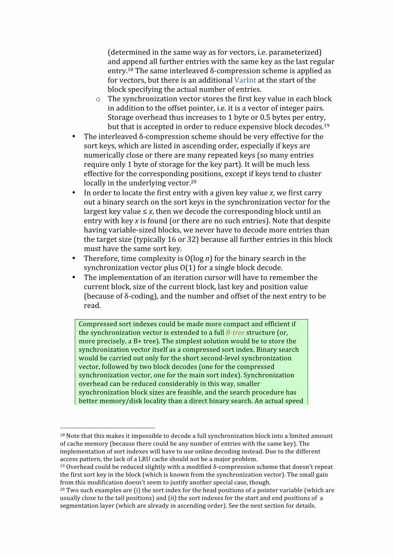
(determined in the same way as for vectors, i.e. parameterized) and append all further entries with the same key as the last regular entry.18 The same interleaved δ-‐compression scheme is applied as for vectors, but there is an additional VarInt at the start of the block specifying the actual number of entries.
o The synchronization vector stores the first key value in each block in addition to the offset pointer, i.e. it is a vector of integer pairs. Storage overhead thus increases to 1 byte or 0.5 bytes per entry, but that is accepted in order to reduce expensive block decodes.19
• The interleaved δ-‐compression scheme should be very effective for the sort keys, which are listed in ascending order, especially if keys are numerically close or there are many repeated keys (so many entries require only 1 byte of storage for the key part). It will be much less effective for the corresponding positions, except if keys tend to cluster locally in the underlying vector.20
• In order to locate the first entry with a given key value x, we first carry out a binary search on the sort keys in the synchronization vector for the largest key value ≤ x, then we decode the corresponding block until an entry with key x is found (or there are no such entries). Note that despite having variable-‐sized blocks, we never have to decode more entries than the target size (typically 16 or 32) because all further entries in this block must have the same sort key.
• Therefore, time complexity is O(log n) for the binary search in the synchronization vector plus O(1) for a single block decode.
• The implementation of an iteration cursor will have to remember the current block, size of the current block, last key and position value (because of δ-‐coding), and the number and offset of the next entry to be read.
Compressed sort indexes could be made more compact and efficient if the synchronization vector is extended to a full B-‐tree structure (or, more precisely, a B+ tree). The simplest solution would be to store the synchronization vector itself as a compressed sort index. Binary search would be carried out only for the short second-‐level synchronization vector, followed by two block decodes (one for the compressed synchronization vector, one for the main sort index). Synchronization overhead can be reduced considerably in this way, smaller synchronization block sizes are feasible, and the search procedure has better memory/disk locality than a direct binary search. An actual speed
18 Note that this makes it impossible to decode a full synchronization block into a limited amount of cache memory (because there could be any number of entries with the same key). The implementation of sort indexes will have to use online decoding instead. Due to the different access pattern, the lack of a LRU cache should not be a major problem. 19 Overhead could be reduced slightly with a modified δ-‐compression scheme that doesn't repeat the first sort key in the block (which is known from the synchronization vector). The small gain from this modification doesn't seem to justify another special case, though. 20 Two such examples are (i) the sort index for the head positions of a pointer variable (which are usually close to the tail positions) and (ii) the sort indexes for the start and end positions of a segmentation layer (which are already in ascending order). See the next section for details.

benefit will have to be demonstrated before we abandon the KISS principle, though.
An inverted index collects the positions of occurrences for each one of a set of types. Usually types are the entries of a given lexicon and positions refer to an underlying data vector, but other applications are also possible. The data structure consists of one sorted list of positions for each type, called a postings list.
• The main access pattern for an inverted index is to obtain all occurrences of a given type, sorted by position, with a cost of O(r). Stream access should be possible in order to avoid large memory buffers for frequent types.
• The implementation should provide similar access to the occurrences of a set of types, sorted into a single list. This is considerably more complex because multiple position streams have to be decoded in parallel and combined by a merge sort. It is difficult to estimate the additional time complexity incurred, though.
• Like a set vector, an inverted index can only be stored in compressed form (because with typical access patterns there are no advantages to uncompressed storage).
• For each type, the postings list is stored as a δ-‐compressed sequence of VarInts (which, by the way, is identical to the special case d=1 of the interleaved δ-‐compression scheme) indicating sequence positions in numerically sorted order.
• If the type is very frequent, an optional jump table can be provided in order to find occurrences within a particular range of positions (e.g. a relatively small subcorpus). The jump table consists of integer (position, offset) pairs, where offset is the byte offset of the VarInt for the next δ increment after position in the main postings list. It is stored in the standard interleaved δ-‐compression scheme for sort index synchronization blocks, starting with a VarInt specifying the number of entries in the table.
• Finally, there is an uncompressed offset table of 3 × k Ints (where k is the number of types), which provides pointers to the main postings lists. Each integer triple describes one type and is interpreted as follows:
o If the type has f ≤ 3, the three integers specify its occurrence positions directly. Empty fields (for f < 3) are padded with –1.
o Otherwise, the first integer holds the value –f, i.e. the negative frequency of the type (negative to distinguish it from a sequence position). The second integer holds the byte offset to the start of the δ-‐compressed postings list for the type. The third integer holds the byte offset to the start of the optional jump table; it is set to –1 if no jump table is present.
• To determine the frequency of a type: o Locate the appropriate entry in the offset table. o If the first integer is negative, flip its sign to obtain the frequency. o Otherwise, compare following integers with –1 to determine
whether frequency is f=1, f=2 or f=3. • To obtain the postings list of a single type:
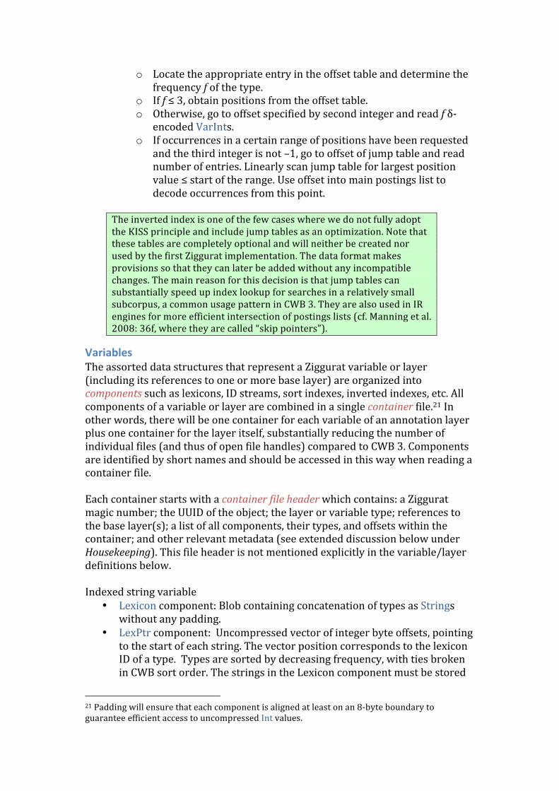
o Locate the appropriate entry in the offset table and determine the frequency f of the type.
o If f ≤ 3, obtain positions from the offset table. o Otherwise, go to offset specified by second integer and read f δ-‐
encoded VarInts. o If occurrences in a certain range of positions have been requested
and the third integer is not –1, go to offset of jump table and read number of entries. Linearly scan jump table for largest position value ≤ start of the range. Use offset into main postings list to decode occurrences from this point.
The inverted index is one of the few cases where we do not fully adopt the KISS principle and include jump tables as an optimization. Note that these tables are completely optional and will neither be created nor used by the first Ziggurat implementation. The data format makes provisions so that they can later be added without any incompatible changes. The main reason for this decision is that jump tables can substantially speed up index lookup for searches in a relatively small subcorpus, a common usage pattern in CWB 3. They are also used in IR engines for more efficient intersection of postings lists (cf. Manning et al. 2008: 36f, where they are called “skip pointers”).
Variables The assorted data structures that represent a Ziggurat variable or layer (including its references to one or more base layer) are organized into components such as lexicons, ID streams, sort indexes, inverted indexes, etc. All components of a variable or layer are combined in a single container file.21 In other words, there will be one container for each variable of an annotation layer plus one container for the layer itself, substantially reducing the number of individual files (and thus of open file handles) compared to CWB 3. Components are identified by short names and should be accessed in this way when reading a container file. Each container starts with a container file header which contains: a Ziggurat magic number; the UUID of the object; the layer or variable type; references to the base layer(s); a list of all components, their types, and offsets within the container; and other relevant metadata (see extended discussion below under Housekeeping). This file header is not mentioned explicitly in the variable/layer definitions below. Indexed string variable
• Lexicon component: Blob containing concatenation of types as Strings without any padding.
• LexPtr component: Uncompressed vector of integer byte offsets, pointing to the start of each string. The vector position corresponds to the lexicon ID of a type. Types are sorted by decreasing frequency, with ties broken in CWB sort order. The strings in the Lexicon component must be stored
21 Padding will ensure that each component is aligned at least on an 8-‐byte boundary to guarantee efficient access to uncompressed Int values.
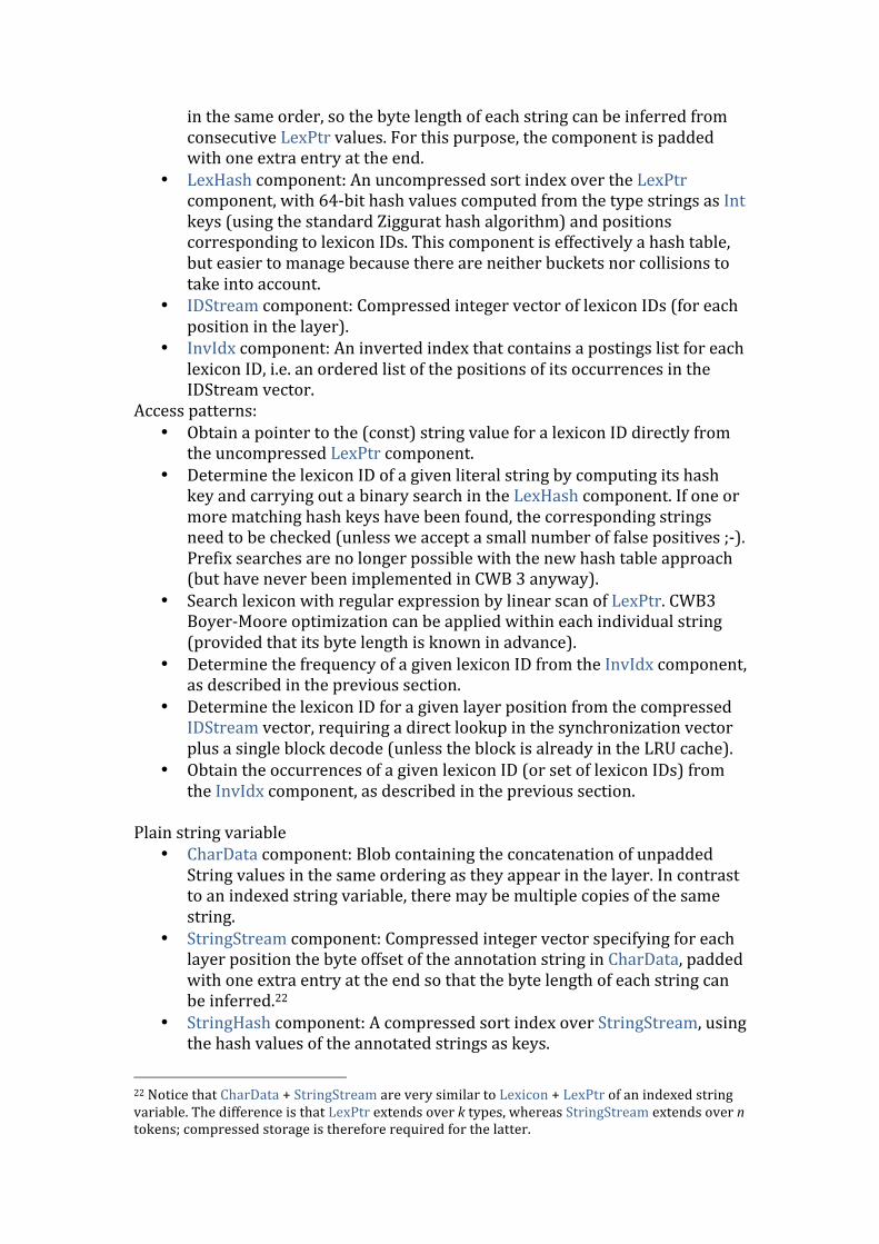
in the same order, so the byte length of each string can be inferred from consecutive LexPtr values. For this purpose, the component is padded with one extra entry at the end.
• LexHash component: An uncompressed sort index over the LexPtr component, with 64-‐bit hash values computed from the type strings as Int keys (using the standard Ziggurat hash algorithm) and positions corresponding to lexicon IDs. This component is effectively a hash table, but easier to manage because there are neither buckets nor collisions to take into account.
• IDStream component: Compressed integer vector of lexicon IDs (for each position in the layer).
• InvIdx component: An inverted index that contains a postings list for each lexicon ID, i.e. an ordered list of the positions of its occurrences in the IDStream vector.
Access patterns: • Obtain a pointer to the (const) string value for a lexicon ID directly from
the uncompressed LexPtr component. • Determine the lexicon ID of a given literal string by computing its hash
key and carrying out a binary search in the LexHash component. If one or more matching hash keys have been found, the corresponding strings need to be checked (unless we accept a small number of false positives ;-‐). Prefix searches are no longer possible with the new hash table approach (but have never been implemented in CWB 3 anyway).
• Search lexicon with regular expression by linear scan of LexPtr. CWB3 Boyer-‐Moore optimization can be applied within each individual string (provided that its byte length is known in advance).
• Determine the frequency of a given lexicon ID from the InvIdx component, as described in the previous section.
• Determine the lexicon ID for a given layer position from the compressed IDStream vector, requiring a direct lookup in the synchronization vector plus a single block decode (unless the block is already in the LRU cache).
• Obtain the occurrences of a given lexicon ID (or set of lexicon IDs) from the InvIdx component, as described in the previous section.
Plain string variable
• CharData component: Blob containing the concatenation of unpadded String values in the same ordering as they appear in the layer. In contrast to an indexed string variable, there may be multiple copies of the same string.
• StringStream component: Compressed integer vector specifying for each layer position the byte offset of the annotation string in CharData, padded with one extra entry at the end so that the byte length of each string can be inferred.22
• StringHash component: A compressed sort index over StringStream, using the hash values of the annotated strings as keys.
22 Notice that CharData + StringStream are very similar to Lexicon + LexPtr of an indexed string variable. The difference is that LexPtr extends over k types, whereas StringStream extends over n tokens; compressed storage is therefore required for the latter.
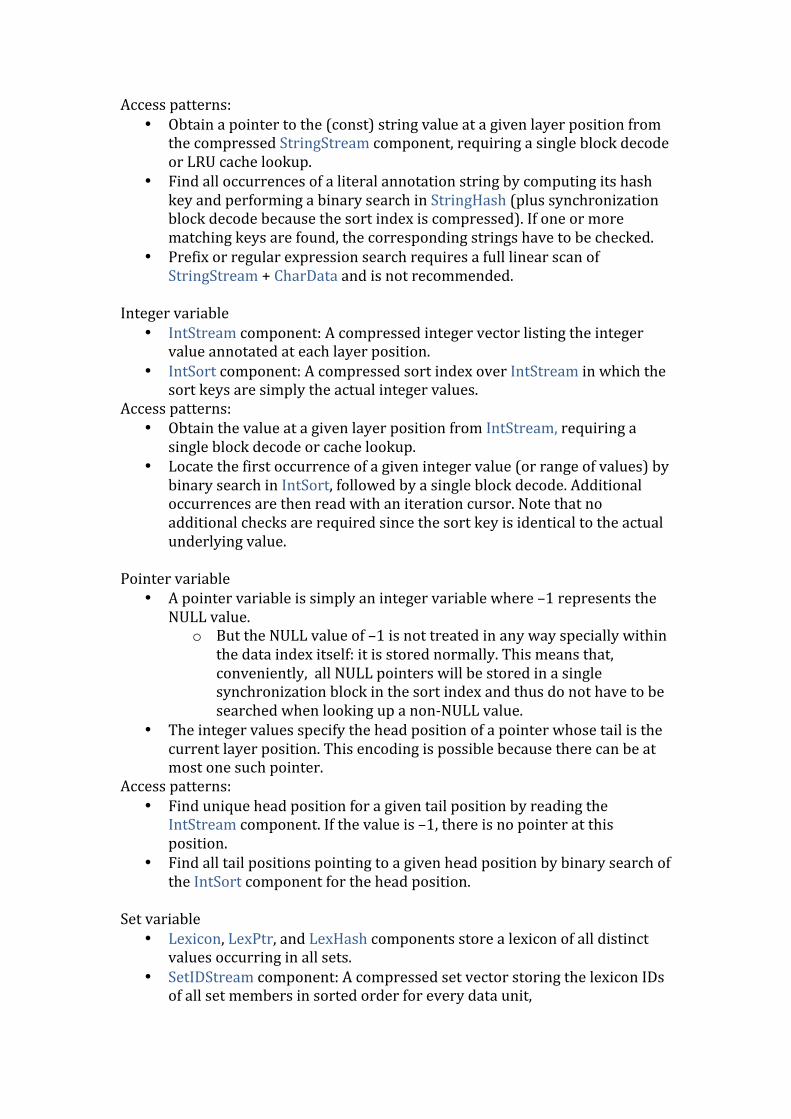
Access patterns: • Obtain a pointer to the (const) string value at a given layer position from
the compressed StringStream component, requiring a single block decode or LRU cache lookup.
• Find all occurrences of a literal annotation string by computing its hash key and performing a binary search in StringHash (plus synchronization block decode because the sort index is compressed). If one or more matching keys are found, the corresponding strings have to be checked.
• Prefix or regular expression search requires a full linear scan of StringStream + CharData and is not recommended.
Integer variable
• IntStream component: A compressed integer vector listing the integer value annotated at each layer position.
• IntSort component: A compressed sort index over IntStream in which the sort keys are simply the actual integer values.
Access patterns: • Obtain the value at a given layer position from IntStream, requiring a
single block decode or cache lookup. • Locate the first occurrence of a given integer value (or range of values) by
binary search in IntSort, followed by a single block decode. Additional occurrences are then read with an iteration cursor. Note that no additional checks are required since the sort key is identical to the actual underlying value.
Pointer variable
• A pointer variable is simply an integer variable where –1 represents the NULL value.
o But the NULL value of –1 is not treated in any way specially within the data index itself: it is stored normally. This means that, conveniently, all NULL pointers will be stored in a single synchronization block in the sort index and thus do not have to be searched when looking up a non-‐NULL value.
• The integer values specify the head position of a pointer whose tail is the current layer position. This encoding is possible because there can be at most one such pointer.
Access patterns: • Find unique head position for a given tail position by reading the
IntStream component. If the value is –1, there is no pointer at this position.
• Find all tail positions pointing to a given head position by binary search of the IntSort component for the head position.
Set variable
• Lexicon, LexPtr, and LexHash components store a lexicon of all distinct values occurring in all sets.
• SetIDStream component: A compressed set vector storing the lexicon IDs of all set members in sorted order for every data unit,
• InvIdx component: An inverted index that contains a postings list for each lexicon ID, i.e. a sorted list of all positions where the corresponding value occurs as a set member. Note that the same position may occur multiple times in the inverted index, once for each member of the set annotated at the position.
Access patterns: • To read the set annotated at a given position, decode the relevant
synchronization block in the SetIDStream, determine the size of the set and the list of lexicon IDs, and obtain (const) pointers to the string values from the LexPtr component.
• Lexicon search (for a specific string or with a regular expression) is carried out in the same way as for an indexed string variable.
• The frequency of a given lexicon ID and its full postings list are obtained from the InvIdx component, in the same way as for an indexed string variable.
• To locate sets containing a given combination of lexicon IDs (i.e. a subset search), a separate postings list for each ID is obtained from InvIdx, then their intersection is computed. A good implementation does not need to materialize the individual lists, but iterates over them in parallel (possibly using jump tables for further optimization). It is also possible to support exclusion constraints (e.g. find all sets that contain A, but not B or C) with the same search strategy.
• It is not possible to know the frequency of a combination of values in advance, as InvIdx only contains frequency information for single IDs.
If sets often contain a relatively large number of members (> 5) but there is only a limited number of distinct sets, the file format of set variables is much less compact and efficient than the CWB3 approach of using and indexed string variable with special set notation. It would be better in these cases to store a list of all distinct sets (in the form of a compressed set vector + inverted index), assigning a unique set ID to each item. The main position stream + inverted index would then just store a single set ID at each position. This complicates the Ziggurat implementation, however, and leads to unnecessary overhead in other situations (with very many distinct sets). If such an extension is defined, it should be optional, i.e. a parameter of the variable. The extension is probably not useful for typical use cases of hash variables. A better solution might be to provide support functions for CWB3-‐like feature set notation, so users can fall back on this approach if a set variable turns out to be too inefficient.
Hash variable
• Keys, KeyPtr, and KeyHash components: a lexicon of all distinct keys. • Values, ValuePtr, and ValueHash components: a lexicon of all distinct
values. • Pairs component: An uncompressed (integer, integer) vector listing all
distinct key-‐value combinations as (key ID, value ID) pairs. Entries are sorted by decreasing frequency of the key-‐value combination (to ensure compact storage in PairsIDStream), with ties broken by key ID, then value ID. The position of a key-‐value combination in this vector is its pair ID.
• PairKeyIdx component: A compressed sort index over the Pairs vector, using the key ID of each pair as a sort key.
• PairValueIdx component: A compressed sort index over the Pairs vector, using the value ID of each pair as a sort key.
• PairIDStream component: A compressed set vector that stores, for each position, the pair IDs of all key-‐value pairs present at this position.
• PairInvIdx component: An inverted index that contains a postings list for each pair ID, i.e. a sorted list of all positions where the corresponding key-‐value combination occurs. Keep in mind that the same position may occur multiple times in the inverted index, once for each key-‐value combination stored in the hash that is annotated at this position.
Access patterns: • The PairIDStream and PairInvIdx components can be understood as a set
variable over key-‐value pairs. Therefore, access patterns are the same as for set variables, with the additional step of determining a pair ID from separate key and value IDs (or vice versa).
• Uncompressed storage of the Pairs component is based on the assumption that the number of distinct key-‐value pairs is not much larger than the size of the values lexicon. It enables fast lookup of the key and value part of a given pair ID. The string representation of a key-‐value pair can be recovered with one direct lookup each in Pairs, KeyPtr and ValuePtr.
• In order to find the pair ID corresponding to a given combination of key ID and value ID, look up the value ID in PairValueIdx and then iterate over all matching pairs until the specified key ID is found. This strategy is based on the assumption that the number of distinct keys is much smaller than the number of distinct values, and that most values will occur only under one or a few keys.
• In order to carry out a regular expression search on the values stored under a particular key, look up the key ID in PairKeyIdx, iterate over all matching pairs in the Pairs vector and apply the regular expression to the corresponding value strings. This strategy is very efficient for keys that take a small set of distinct values because only these values need to be matched against the regular expression. Occurrences of the resulting list of pair IDs are then determined by computing the union of their respective postings lists.
• As for set variables, it is not possible to know the “joint” frequency of a given combination of key-‐value pairs without computing the intersection of their position lists. The frequency of their union – which arises e.g. in the case of a regular expression search under a particular key described in the previous item – can easily be determined if the key-‐value pairs are known to be mutually exclusive (in particular, if each key may appear at most once per hash).
Layers Primary layer
• Does not require base-‐layer reference data, so there are no additional data structures after the container file header.
• A primary layer simply provides a virtual sequence of positions (data units) to which variables can refer.
Segmentation layer
• Ranges component: A compressed (integer, integer) vector representing ranges in the base layer as pairs of (start, end+1) positions, i.e. using the Python indexing scheme.23 Ranges are sorted by increasing start position They must not overlap or nest, and cannot be empty in a segmentation layer.
• StartIdx component: A compressed sort index over the Ranges vector with the start position of each range as integer key.
• EndIdx component: A compressed sort index over the Ranges vector with the end+1 position of each range as integer key.
Access patterns: • Obtain start and end position of the i-‐th range from Ranges component.
Find unique range enclosing a given position p in the base layer by binary search of the StartIdx component for the last range starting before p; then check whether this range in fact contains p.
• The StartIdx and EndIdx components are used to check quickly, i.e. in O(log n) time, if a given base layer position is the start or end of a region, which is frequently needed in CQP 3. Binary search on the compressed Ranges vector would be extremely inefficient.
Tree layer:
• Ranges component similar to segmentation layer. Ranges may be nested hierarchically and empty ranges are expressly allowed, but there must not be any crossing brackets. Ranges are ordered according to their start tags in an XML serialization, which corresponds to a pre-‐order traversal of the tree.24
• StartIdx component as in segmentation layer. • EndIdx component as in segmentation layer. • In addition, every tree layer has two special pointer variables, which are
referred to as _parent and _next in this document.25 For each element of the tree (i.e. data unit in the tree layer), they point to the parent element (_parent) and the following sibling (_next), respectively.
Access patterns: • Obtain start and end position of the i-‐th range from Ranges component. • Finding the lowest element in the tree that encloses a given position x in
the base layer is quite tricky. First, use StartIdx to find the last element e 23 Python indexing is used for two reasons: (i) it simplifies some computations, such as the length of a range or splitting ranges in a binary search; (ii) the encoding of empty ranges as (i, i) seems more natural than (i, i–1) according to the CWB3 indexing scheme. 24 An earlier version of this document specified that ranges should be ordered by increasing start position, then decreasing end position. This is equivalent to the new ordering by start tags unless there are (i) empty ranges or (ii) multiple ranges with the same start and end position. 25 Of course, they don't really have names but are rather identified by UUID, so there is no risk of a collision with user-‐defined variables.
with start position ≤ x; this element must be a descendant of all elements that contain x. If e contains x, it is the desired element. Otherwise, follow the _parent pointers until an element containing x is found or no such element exists.
• Navigating the element tree is easy by forward and backward traversal of the _parent and _next pointers. Note that the ordering rules for sort indexes ensure that backward traversal of _parent returns children in their corpus order (by start tag).
• All start tags at a given base layer position can easily be found through the StartIdx sort index. They are already listed in the correct order in the Ranges component.
• All end tags at a given base layer position can be found through the EndIdx sort index. For non-‐empty elements, they are returned in reverse order, i.e. the last end tag (corresponding to the earliest start tag) is returned first. The precise position of empty elements can only be determined by traversing the tree structure. For example, the sort order doesn't distinguish between <a/><b/> and <a><b/></a>.
• Reconstructing the original XML tags is fairly tricky and will require many special cases for correct positioning of empty elements. This is left as an exercise to the poor sod implementing the Ziggurat library.
Graph layer:
• Edges component: A compressed integer vector of (tail, head) pairs, where tail is the position of the edge in the source base layer and head its position in the target base layer. Data units are ordered by increasing tail position first, then increasing head position.
• TailIdx component: A compressed sort index over the Edges vector using tail position as integer key.
• HeadIdx component: A compressed sort index over the Edges vector using head position as integer key.
Access patterns: • The tail and head position of a given edge are obtained from Edges. • Find all edges starting from a given tail position in the source base layer
through binary search of the TailIdx sort index. The corresponding head positions then have to be read from Edges. If there are multiple edges, they are adjacent in the Edges component and can be accessed without much overhead.
• Find all edges ending in a given head position in the target base layer through binary search of the HeadIdx sort index. The corresponding tail positions then have to be read from the Edges component, where they will usually not be adjacent.
The current design of graph layers leaves much room for optimization. For graphs with many edges, the duplication of head and tail positions in HeadIdx and TailIdx may be wasteful. Traversing the graph is expensive because each step requires a O(log n) binary search in TailIdx or HeadIdx, followed by a lookup of the corresponding head or tail position in the Edges component (which may result in an additional block decode). Checking relation labels requires yet another access to a

compressed vector in the corresponding indexed string variable. Graph layers are thus a primary candidate for more specialized data structures.
Housekeeping Container files have to include a header listing
• their random UUID, • the layer or variable type, • a bill of materials (see definition below) for each component, • and perhaps further information.
Ziggurat containers should be self-‐describing, i.e. they should contain a complete bill of materials (BOM), listing for each component
• the component name (NUL-‐terminated string); • the type of the component and its parameters if applicable (e.g. the
number d of integers in each element of a vector, the size of synchronization blocks, etc.);
• the byte offset and length of the component. Such a BOM opens the possibility of user-‐defined container types, which don't need to be declared specially. Applications can simply check whether the expected components are present and have appropriate types; they can use low-‐level functions in the Ziggurat library to access the individual components (as described above). User-‐defined containers would not complicate the implementation of Ziggurat and CWB 4 in any way. The normal API functions only accept standard containers (i.e. those declared with a standard type). The BOM provides additional safety since (a) components are accessed by name rather than an implicitly defined ordering and (b) component types can be verified.