Predictability of Interest Rates and Interest-Rate Portfolios∗

TURAN BALI †

Zicklin School of Business, Baruch College

MASSED HEIDARI‡

Caspian Capital Management, LLC

L IUREN WU§

Zicklin School of Business, Baruch College

First draft: June 21, 2003

This version: June 14, 2006

∗We thank Yacine Aıt-Sahalia, David Backus, Peter Carr, Silverio Foresi, Gregory Klein, Karl Kolderup, Bill Lu, and seminarparticipants at Baruch College, the City University of HongKong, Goldman Sachs, and the 2004 China International Confer-ence in Finance for helpful suggestions and discussions. Wewelcome comments, including references to related papers we haveinadvertently overlooked.

†One Bernard Baruch Way, Box B10-225, New York, NY 10010; tel:(646) 312-3506; fax: (646) 312-3451;Turan Bali@baruch.cuny.edu.

‡745 Fifth Avenue, 28th floor, New York, NY 10151; tel: (212) 703-0333; fax: (212) 703-0380;Massoud.Heidari@caspiancapital.com.

§One Bernard Baruch Way, Box B10-225, New York, NY 10010; tel:(646) 312-3509; fax: (646) 312-3451;Liuren Wu@baruch.cuny.edu; http://faculty.baruch.cuny.edu/lwu/.

Predictability of Interest Rates and Interest-Rate Portfolios

ABSTRACT

Due to the near unit-root behavior of interest rates, the movements of individual interest-rate series

are inherently difficult to forecast. In this paper, we propose an innovative way of applying dynamic

term structure models to forecast interest-rate movements. Instead of directly forecasting the movements

based on the estimated factor dynamics, we use the dynamic term structure model as a decomposition

tool and decompose each interest-rate series into two components: a persistent component captured

by the dynamic factors, and a strongly mean-reverting component given by the pricing residuals of

the model. With this decomposition, we form interest-rate portfolios that are first-order neutral to the

persistent dynamic factors, but are fully exposed to the strongly mean-reverting residuals. We show that

the predictability of these interest-rate portfolios is significant both statistically and economically, both

in sample and out of sample.

JEL Classification:E43; G11; G12; C51.

Keywords:Term structure; Predictability; Interest rates; Factors;Pricing errors; Expectation hypotheses.

Predictability of Interest Rates and Interest-Rate Portfolios

Forecasting interest-rate movements attracts great attention from both academics and practitioners. A central

theme underlying the traditional literature is to exploit the information content in the current term structure to

forecast the future movement of interest rates. These studies formulate forecasting relations based on various

forms of the expectation hypothesis.1 More recently, several researchers apply the theory of dynamic term

structure models in further understanding the links between the cross-sectional behavior (term structure)

of interest rates and their time-series dynamics. They propose and test model specifications that can best

explain the empirical evidence on the expectation hypothesis and the properties of excess bond returns.2 In

this paper, we propose a new way of applying multivariate dynamic term structure models in forecasting

interest-rate movements.

Modern dynamic term structure models accommodate multipledynamic factors in governing the interest-

rate movements. Several empirical studies also identify nonlinearity in the interest-rate dynamics.3 Thus,

if the focus is on forecasting, a better formulation should be in a multivariate framework, and potentially

in nonlinear forms, rather than in the form of simple linear regressions designed to verify the expectation

hypothesis and the behavior of market risk premium. Furthermore, if interest rates are composed of multiple

factors, do these factors exhibit the same predictability?If not, can we separately identify these factors

from the interest-rate series and forecast only the more predictable components while hedging away the less

predictable ones?

We address these questions based on weekly data on 12 eurodollar LIBOR and swap rate series from

May 11, 1994 to December 10, 2003 at maturities from one monthto 30 years. We perform our analysis

within the framework of three-factor affine dynamic term structure models. We apply the unscented Kalman

filter to estimate the term structure models and to extract the interest-rate factors and the pricing errors.

Similar to earlier findings in the literature, we observe that the estimated three interest-rate factors are

1Prominent examples include Roll (1970), Fama (1984), Fama and Bliss (1987), Mishkin (1988), Fama and French (1989, 1993),Campbell and Shiller (1991), Evans and Lewis (1994), Hardouvelis (1994), Campbell (1995), Bekaert, Hodrick, and Marshall(1997, 2001), Longstaff (2000), Bekaert and Hodrick (2001), and Cochrane and Piazzesi (2005).

2See, for example, Backus, Foresi, Mozumdar, and Wu (2001), Dai and Singleton (2002), Duffee (2002), and Roberds andWhiteman (1999).

3Examples include Aıt-Sahalia (1996a,b), Stanton (1997),Chapman and Pearson (2000), Jones (2003), and Hong and Li (2005).

1

highly persistent. When we try to forecast four-week ahead interest-rate changes based on the estimated

factor dynamics, the performance is no better than the basicassumption of random walk.

In pricing 12 interest rate series with three factors, we will observe pricing errors. The unscented Kalman

filter estimation technique accommodates these pricing errors in the form of measurement errors. Thus, the

estimation procedure decomposes each interest-rate series into two components: the model-implied fair

value as a function of the three factors, and the pricing error that captures the idiosyncratic movement of

each interest-rate series. We can think of the pricing errors as the higher dimensional dynamics that are not

captured by the three factors. Compared to the highly persistent interest-rate factors, we find that the pricing

errors on the interest-rate series are strongly mean reverting.

Based on this observation, we propose a new way of applying the dynamic term structure models in fore-

casting interest-rate movements. Instead of using the estimated dynamic factors to forecast the movements

of each individual interest-rate series, we use the model asa decomposition tool. We form interest-rate

portfolios that are first-order neutral to the persistent interest-rate factors, but are fully exposed to the more

mean-reverting idiosyncratic components. To illustrate the idea, we use swap rates at two-, five-, ten-, and

30-year maturities to form such a portfolio. We find that, in contrast to the low predictability of the indi-

vidual swap rate series, the portfolio shows strong predictability. For example, in forecasting interest-rate

changes over a four-week horizon based on an AR(1) specification, we obtain R-squares less than 2% for all

12 individual interest-rate series. In contrast, the forecasting regression on the swap-rate portfolio generates

an R-square of 14%.

To generalize, we use the 12 interest-rate series to form 495different combinations of four-instrument

interest-rate portfolios that are hedged with respect to the three persistent interest-rate factors. We find

that all these 495 portfolios show strong predictability. The R-squares from the AR(1) forecasting regres-

sion range from 7.84% to 55.72%, with an average of 19.32%, illustrating the robustness of the portfolio-

construction strategy in enhancing the predictability of the portfolio return.

We use the same idea to form two-instrument interest-rate portfolios to hedge away the most persistent

interest-rate factor, and three-instrument interest rateportfolios to hedge away the first two factors. We find

that the predictability of most of the two- and three-instrument portfolios remains weak, indicating that we

must hedge away all the first three factors to generate portfolios with strong predictability.

2

To investigate the economic significance of the predictability of the four-instrument interest-rate portfo-

lios, we follow the practice of Kandel and Stambaugh (1996) and devise a simple mean-variance investment

strategy on the four-instrument portfolios over a four-week horizon that exploits the portfolios’ strong pre-

dictability. During our sample period, the investment exercise generates high premiums with low standard

deviation. The annualized information ratio estimates range from 0.36 to 0.94, with an average of 0.7, illus-

trating the strong economic significance of the predictability of the four-instrument portfolios. Furthermore,

the excess returns from the investment exercise show positive skewness, and the average positive premi-

ums cannot be fully explained by systematic factors in the stock, corporate bond, and interest-rate options

markets.4 Given their independence of systematic market factors, we hypothesize that the average positive

excess returns are premiums to bearing short-term liquidity shocks to individual interest-rate swap contracts.

We construct measures that proxy the absolute magnitudes ofcontract-specific liquidity shocks in the swap

market and find that larger liquidity shocks at a given date often lead to more positive excess returns ex post

for investments put on that day.

The literature has linked the three persistent interest-rate factors to systematic movements in macroeco-

nomic variables such as the long-run expected inflation rate, the output gap, and the short-run Fed policy

shocks. Within a short investment horizon, e.g., four weeks, these systematic movements are difficult to

predict. The four-instrument interest-rate portfolios that we have constructed in this paper are relatively

immune to these persistent and systematic movements, but are exposed to more transient shocks due to tem-

porary supply-demand variations. Trading against these shocks amounts to providing short-term liquidity

to the market and hence bearing a transient liquidity risk. Our analysis shows that historically the swap

market has assigned a relatively high average premium to theliquidity risk, potentially due to high barriers

to entry, limits of arbitrage, and compensation for intellectual capital (Duarte, Longstaff, and Yu (2005)).

Our subsample analysis further shows that the risk premium has declined over the past few years, a sign

of increasing liquidity and efficiency in the interest-rateswap market. Nevertheless, the predictability of

our four-instrument interest-rate portfolios remains much stronger than that of individual interest-rate series

4The high information ratios and positive skewness are also observed in excess returns on popular fixed income arbitragestrategies (Duarte, Longstaff, and Yu (2005)). In contrast, excess returns from other high-information-ratio investment strate-gies reported in the literature often exhibit negatively skewed distributions, e.g., selling out-of-the-money put options (Coval andShumway (2001), Goetzmann, Ingersoll, Spiegel, and Welch (2002)), shorting variance swap contracts (Carr and Wu (2004)), andmerger arbitrage (Mitchell and Pulvino (2001)).

3

across different sample periods, both in sample and out of sample. Furthermore, our results are robust to

different model specifications within the three-factor affine class.

Our new application of the dynamic term structure models sheds new insights for future interest-rate

modeling. The statistical and economic significance of the predictability of the interest-rate portfolios point

to a dimension of deficiency in three-factor dynamic term structure models. These models capture the

persistent movements in interest rates, but discard the transient interest-rate movements. Yet, not only

can these transient movements be exploited in investment decisions to generate economically significant

premiums, as we have shown in this paper, but they can also play important roles in valuing interest-rate

options (Collin-Dufresne and Goldstein (2002) and Heidariand Wu (2002, 2003)) and in generating the

observed low correlations between non-overlapping forward interest rates (Dai and Singleton (2003)).

The remainder of this paper is structured as follows. Section 1 describes the specification and estimation

of the three-factor affine dynamic term structure models that underlie our analysis. We also describe the data

and estimation methodology, and summarize the estimation relevant results in this section. Section 2 inves-

tigates the statistical significance of the predictabilityof interest rates and interest-rate portfolios. Section 3

studies the economic significance of the interest-rate portfolios from an asset-allocation perspective. Sec-

tion 4 performs robustness analysis by examining the predictability variation across different subsamples, in

sample and out of sample, and under different model specifications. Section 5 concludes.

1. Specification and Estimation of Affine Dynamic Term Structure Models

We perform our analysis based on affine dynamic term structure models (Duffie and Kan (1996) and Duffie,

Pan, and Singleton (2000)). The specification and estimation of affine term structure models have been

studied extensively in the literature, e.g., Backus, Foresi, Mozumdar, and Wu (2001), Dai and Singleton

(2000, 2002), Duffee (2002), and Duffee and Stanton (2000).We follow these works in specifying and

estimating a series of standard three-factor models in thissection. However, our proposed applications of

the estimated models in the subsequent sections are completely different from the previous studies.

4

1.1. Model specification

To fix notation, we consider a filtered complete probability spaceΩ,F ,P,(F t)0≤t≤T that satisfies the

usual technical conditions withT being some finite, fixed time. We useX ∈ Rn to denote ann-dimensional

vector Markov process that represents the systematic stateof the economy. We assume that for any time

t ∈ [0,T ] and maturing dateT ∈ [t,T ], the fair value at timet of a zero-coupon bond with time-to-maturity

τ = T − t is fully characterized byP(Xt,τ) and that the instantaneous interest rater is defined by continuity:

r (Xt) ≡ limτ↓0

− lnP(Xt,τ)τ

. (1)

We further assume that there exists a risk-neutral measureP∗ such that the fair values of the zero-coupon

bonds and future instantaneous interest rates are linked asfollows,

P(Xt ,τ) = E∗t

[

exp

(

−Z t+τ

tr(Xs)ds

)]

, (2)

whereE∗t [·] denotes the expectation operator under measureP

∗ conditional on the filtrationF t .

Under the affine class, the instantaneous interest rate is anaffine function of the state vector,

r(Xt) = ar +b⊤r Xt , (3)

and the state vector follows affine dynamics under the risk-neutral measureP∗,

dXt = κ∗ (θ∗−Xt)dt+√

StdW∗t , (4)

whereSt is a diagonal matrix with itsith element given by

[St ]ii = αi + β⊤i Xt, (5)

5

with αi being a scalar andβi an n-dimensional vector. Under these specifications, the fair-values of the

zero-coupon bonds are exponential affine in the state vectorXt ,

P(Xt ,τ) = exp(

−a(τ)−b(τ)⊤Xt

)

, (6)

where the coefficients can be solved from a set of ordinary differential equations (Duffie and Kan (1996)).

Dai and Singleton (2000) classify the affine models into a canonicalAm(n) structure such that

[St ]ii =

Xt,i i = 1, · · · ,m;

1+ β⊤i Xt, i = m+1, · · · ,n,

(7)

βi = [βi1, · · · ,βim,0, · · · ,0]⊤ . (8)

The normalization amounts to settingαi = 0 andβi = 1i for i ≤ m, where 1i denotes a vector with itsith

element being one and other elements being zero. In essence,the firstm factors follow square-root dynamics.

To derive the state dynamics under the physical measureP, Dai and Singleton (2000) assume that the

market price of risk is proportional to√

St , γ(Xt) =√

Stλ1, whereλ1 is ann×1 vector of constants. Duffee

(2002) proposes a more general specification,

γ(Xt) =√

Stλ1 +

√

S−t λ2Xt , (9)

whereλ2 is ann×n matrix of constants andS−t is a diagonal matrix with itsith diagonal element given by

[S−t ]ii =

0, i = 1, · · · ,m;(

1+ β⊤i Xt

)−1, i = m+1, · · · ,n.

(10)

Under the general market price of risk specification in (9), theP-dynamics of the state vector remains affine,

dXt = κ(θ−Xt)dt+√

StdWt , (11)

6

with

[κθ]i = [κ∗θ∗]i +

0, i = 1, · · · ,m;

λ1,i i = m+1, · · · ,n,(12)

κi,· = κ∗i,·−

λ1,i1⊤i , i = 1, · · · ,m;(

λ1,iβ⊤i + λ2,i

)

i = m+1, · · · ,n,(13)

whereκi,· andλ2,i denote theith row ofκ andλ2, respectively, andλ1,i denotes theith element of the vector.

Since the firstm rows ofλ2 do not enter the dynamics ofX, we normalizeλ2,i = 0 for i = 1, · · · ,m.

For our analysis, we follow the common practice in the literature in focusing on three-factor models. We

estimate four genericAm(3) models withm= 0,1,2,3 and with the general market price of risk specification

in equation (9). In the case ofm = 0, St and S−t become identity matrices. The three factors follow a

multivariate Ornstein-Uhlenbeck process,

dXt = −κXtdt+dWt , (14)

where we normalize the long-run meanθ = 0. For identification purpose, we restrict theκ matrix to be lower

triangular. In this case, the essentially affine market price of risk specification in equation (9) becomes

γ(Xt) = λ1 + λ2Xt , (15)

so that the risk-neutral state dynamics becomes

dXt = κ∗ (θ∗−Xt)dt+dW∗t , κ∗θ∗ = −λ1, κ∗ = κ+ λ2. (16)

We also confineλ2 and henceκ∗ to be lower triangular. ForAm(3) models withm= 1,2,3, we normalize

θ∗i = 0 for i = m+1,c. . . ,n. We also normalizeκ∗ andκ to be lower triangular matrices.

7

1.2. Data and estimation

We estimate the four affine dynamic term structure models andanalyze the predictability of interest rates

based on five eurodollar LIBOR and seven swap rate series. TheLIBOR rates have maturities at one, two,

three, six and 12 months, and the swap rates have maturities at two, three, five, seven, ten, 15, and 30 years.

For each rate, the Bloomberg system computes a composite quote based on quotes from several broker

dealers. We use the mid quotes of the Bloomberg composite formodel estimation. The data are sampled

weekly (every Wednesday) from May 11, 1994 to December 10, 2003, 501 observations for each series.

LIBOR rates are simply compounded interest rates, relatingto the values of the zero-coupon bonds by,

LIBOR(Xt,τ) =100

τ

(

1P(Xt,τ)

−1

)

, (17)

where the time-to-maturityτ is computed based on actual over 360 convention, starting two business days

forward. The swap rates relate to the zero-coupon bond prices by,

SWAP(Xt ,τ) = 100h× 1−P(Xt,τ)∑hτ

i=1P(Xt , i/h), (18)

whereτ denotes the maturity of the swap andh denotes the number of payments in each year. For the

eurodollar swap rates that we use, the number of payments is twice per year,h = 2, and the day counting

convention is 30/360.

Table 1 reports the summary statistics of the 12 LIBOR and swap rates. The average interest rates

have an upward sloping term structure. The standard deviation of the interest rates shows a hump-shaped

term structure that reaches its plateau at one-year maturity. All interest-rate series show small estimates for

skewness and excess kurtosis.

The interest rates are highly persistent. The first-order weekly autocorrelation ranges from 0.985 to

0.995, with an average of 0.991. An AR(1) dynamics approximates well the autocorrelation function at

higher orders. If we assume an AR(1) dynamics for interest rates, an average weekly autocorrelation esti-

mate of 0.991 implies a half life of 78 weeks.5 Therefore, if we make forecasting and investment decisions

5We define the half life as the number of weeks for the weekly autocorrelation (φ) to decay to half of its first-order value:Half-life (in weeks) = ln(φ/2)/ ln(φ).

8

based on the mean-reverting properties of interest rates, we need a very long investment horizon for the

mean reversion to actually materialize.

We cast the four dynamic term structure models into state-space forms and estimate the model parame-

ters using the quasi-maximum likelihood method based on observations on the 12 interest-rate series. Under

this estimation technique, we regard the three interest-rate factors as unobservable states and the LIBOR and

swap rates as observations. The state propagation equationfollows a discrete-time version of equation (11),

Xt+1 = A+ ΦXt +√

Q tεt+1, (19)

whereε ∼ IIN (0, I), Φ = exp(−κ∆t) with ∆t = 1/52 as the discrete-time (weekly) interval,A = θ(I −Φ),

andQt = St∆t.

We define the measurement equation using the 12 LIBOR and swaprates, assuming additive and

normally-distributed measurement errors,

yt =

LIBOR(Xt, i)

SWAP(Xt , j)

+et , cov(et ) = R ,i = 1,2,3,6,12 months

j = 2,3,5,7,10,15,30 years.(20)

For the estimation, we assume that the measurement errors oneach series are independent but with distinct

variance:R ii = σ2i andR i j = 0 for i 6= j.

When both the state propagation equation and the measurement equations are Gaussian and linear, the

Kalman (1960) filter generates efficient forecasts and updates on the conditional mean and covariance of

the state vector and the measurement series. In our application, the state propagation equation in (19) is

Gaussian and linear, but the measurement equation in (20) isnonlinear. We use the unscented Kalman

filter (Wan and van der Merwe (2001)) to handle the nonlinearity. The unscented Kalman filter directly

approximates the posterior state density using a set of deterministically chosen sample points (sigma points).

These sample points completely capture the true mean and covariance of the Gaussian state variables, and

when propagated through the nonlinear functions of LIBOR and swap rates, capture the posterior mean and

covariance accurately to the second order for any nonlinearity.

9

Let yt+1 andAt+1 denote the time-t ex ante forecasts of time-(t + 1) values of the measurement series

and the covariance of the measurement series obtained from the unscented Kalman filter, we construct the

log-likelihood value assuming normally distributed forecasting errors,

lt+1(Θ) = −12

log∣

∣At

∣

∣− 12

(

(yt+1−yt+1)⊤ (

At+1)−1

(yt+1−yt+1))

. (21)

The model parameters are chosen to maximize the log likelihood of the data series,

Θ ≡ argmaxΘL (Θ,ytN

t=1), with L (Θ,ytNt=1) =

N−1

∑t=0

lt+1(Θ), (22)

whereN = 501 denotes the number of weeks in our sample of estimation.

1.3. The dynamics of interest-rate factors and pricing errors

The model specifications and estimations are relatively standard, and our results are also similar to those

reported in the literature. Since all four models generate similar performance, our conclusions are not

particularly sensitive to the exact model choice. For expositional clarity, we henceforth focus our discussions

on theA0(3) model, and address the similarities and differences of the other three models,Am(3),m= 1,2,3,

in a separate section. From the estimated models, we analyzethe dynamics of the interest-rate factors and the

behavior of the pricing errors, both of which are important for our subsequent analysis on the predictability

of interest rates and interest-rate portfolios.

1.3.1. Factor dynamics

Table 2 reports the parameter estimates and the absolute magnitudes of thet-values for theA0(3) model.

The parameter estimates onκ control the mean-reverting feature of the time-series dynamics of the three

Gaussian factors. For the factor dynamics to be stationary,the real parts of the eigenvalues of theκ matrix

must be positive. Under the lower triangular matrix assumption, the eigenvalues of theκ matrix coincide

with the diagonal elements of the matrix.

10

The estimate for the first diagonal element is very small at 0.002. Itst-value is also very small, implying

that the estimate is not statistically different from zero.Hence, the first factor is close to being nonstationary.

The estimate for the second eigenvalue is 0.48, with at-value of 1.19, and hence not significantly different

from zero. The estimate for the third eigenvalue of theκ matrix is significantly different from zero, but

the magnitude remains small at 0.586, indicating that all three factors are highly persistent. The largest

eigenvalue of 0.586 corresponds to a weekly autocorrelation of 0.989, and a half life of 62 weeks.

Theκ∗ matrix represents the counterpart ofκ under the risk-neutral measure. The estimates forκ∗ are

close to the corresponding estimates forκ, indicating that the three interest-rate factors also showhigh per-

sistence under the risk-neutral measure. Compared to theκ matrix, which controls the time-series dynamics

of the interest rates, the risk-neutral counterpartκ∗ controls the cross-sectional behavior (term structure) of

interest rates. Thet-values forκ∗ are much larger than thet-values for the corresponding elements ofκ.

Thus, by estimating the dynamic term structure model on the interest-rate data, we can identify the risk-

neutral dynamics and hence capture the term structure behavior of interest rates much more accurately than

capturing the time-series dynamics.

The difference int-values betweenκ andκ∗ also implies that from the perspective of a dynamic term

structure model, forecasting future interest-rate movements is more difficult than fitting the observed term

structure of interest rates. This difficulty is closely linked to the near unit-root behavior of interest rates. The

difficulty in forecasting persists even if we perform the estimation on the panel data of interest rates across

different maturities and hence exploit the full information content of the term structure.

1.3.2. Properties of pricing errors

In using a three-factor model to fit the term structure of 12 interest rates, we will see discrepancies between

the observed interest rates and the model-implied values. In the language of the state-space model, the

differences between the two are called measurement errors.They can also be regarded as the model pricing

errors. The unscented Kalman filter minimizes the pricing errors in a least square sense.

Table 3 reports the sample properties of the pricing errors.The sample mean shows the average bias be-

tween the observed rates and the model-implied rates. The largest biases come from the six- and 12-month

11

LIBOR rates, potentially due to margin differences and quoting non-synchronousness between LIBOR and

swap rates (James and Webber (2000)). The root mean squared pricing error (rmse) measures the relative

goodness-of-fit on each series. The largest root mean squared error comes from the 12-month LIBOR rate

at 14.145 basis points. The maximum absolute pricing error is 60.495 basis points on the one-month LI-

BOR rate. The skewness and excess kurtosis estimates are much larger than the corresponding estimates

on the original interest rates, especially for the short-term LIBOR rates, reflecting the occasionally large

mismatches between the model and the market at the short end of the yield curve (Heidari and Wu (2003b)).

Overall, the model captures the main features of the term structure well. The last column reports the ex-

plained percentage variation (VR) on each series, defined asone minus the ratio of pricing error variance to

the variance of the original interest-rate series, in percentage points. The estimates suggest that the model

can explain over 99% of the variation for 11 of the 12 interest-rate series.

We also report the weekly autocorrelation for the pricing errors. The autocorrelation is smaller for the

better-fitted series. The average weekly autocorrelation for the pricing errors is at 0.69, much smaller than

the average of 0.991 for the original interest-rate series.Based on an AR(1) structure, a weekly autocorrela-

tion of 0.69 corresponds to a half life of less than three weeks, much shorter than the average half life for the

original series. Thus, if we can make an investment on the pricing errors instead of on the original interest-

rate series, our ability to forecast will become much stronger and convergence through mean-reversion will

become much faster.

2. Predictability of Interest-Rate Portfolios

Given the estimated dynamic term structure models, a traditional approach is to directly predict future

interest-rate movements based on the estimated factor dynamics, e.g., Duffee (2002) and Duffee and Stanton

(2000). We start this section by repeating a similar exercise as a benchmark for comparison. We then propose

a new, innovative application of the estimated dynamic termstructure models to enhance the predictability.

In this new application, we do not use the estimated factor dynamics to directly predict interest-rate move-

ments, but use the model as a decomposition tool and form interest-rate portfolios that are significantly more

predictable than are the individual interest-rate series.

12

2.1. Forecasting interest rates based on estimated factor dynamics: A benchmark

As a benchmark for our subsequent analysis, we forecast eachLIBOR and swap rate series using the esti-

matedA0(3) model via the following procedure. At each date, based on theupdates on the three factors,

we forecast the values of the three factors four weeks ahead according to the state propagation equation in

(19) and with the time horizon∆t = 4/52. The choice of a four-week forecasting horizon is a compromise

between the weekly data used for model estimation and a reasonably long horizon for forecasting. Given

the high persistence in interest rates, the investment horizon is usually one month or longer.

Using the forecasts on the three factors, we compute the forecasted values of zero-coupon bond prices

according to equation (6) and the forecasted LIBOR and swap rates according to equations (17) and (18).

Then, we compute the forecasting error as the difference in basis points between the realized LIBOR and

swap rates four weeks later and the forecasted values.

We compare the forecasting performance of theA0(3) model with two alternative strategies: the random

walk hypothesis (RW), under which the four-week ahead forecast of the LIBOR and swap rate is the same

as the current rate, and a first-order autoregressive regression (OLS) on the LIBOR or swap rate over a

four-week horizon.

Table 4 reports the sample properties of the four-week aheadforecasting error from the three forecasting

strategies. By design, the in-sample forecasting error from the regression is always smaller in the least

square sense than that from the random walk hypothesis. However, due to the high persistence of interest

rates, the differences between the sample properties of theforecasting errors from RW and OLS are very

small. The root mean squared forecasting errors on each series from the two strategies are less than half a

basis point apart. In the last column in each panel, we reportthe explained percentage variation, defined as

one minus the variance of the forecasting errors over the variance of the four-week changes in the interest

rate series. By definition, the random walk strategy has zeroexplanatory power on the changes in LIBOR

and swap rates. The OLS strategy generates positive results, but the outperformance is very small, with

the highest percentage being 1.528% for the 30-year swap rates. Hence, for short-term investment over a

horizon of four weeks, the gain from exploiting the mean-reverting property of individual interest-rate series

is negligible, even for in-sample analysis.

13

The last panel reports the properties of the forecasting errors from theA0(3) dynamic term structure

model. The model’s forecasting performance is not significantly better than the simple random walk hy-

pothesis. In fact, the root mean squared error from the modelis larger than the mean absolute forecasting

error from the random walk hypothesis for seven of the 12 series, and the explained variation estimates

are negative for eight of the 12 series. Therefore, the dynamic term structure model delivers poor forecast-

ing performance. Duffee (2002) and Duffee and Stanton (2000) observe similar performance comparisons

for a number of different dynamic term structure models, reflecting the inherent difficulty in forecasting

interest-rate movements using multi-factor dynamic term structure models.

2.2. Forming interest-rate portfolios that are strongly predictable

Given the near unit-root behavior of interest rates, neither dynamic term structure models nor autoregressive

regressions can do much better than a simple random walk assumption in predicting future changes in the

individual interest-rate series. However, the pricing errors from the dynamic term structure models show

much smaller persistence than both the interest-rate factors and the original interest-rate series. As a result,

an autoregressive regression can predict future changes inthe pricing errors much better than does the

random walk hypothesis. Therefore, the predictable component in the interest-rate movements is not in the

estimated dynamic factors, but in the pricing errors. Basedon this observation, we propose a new way of

applying the term structure model in forecasting interest rates.

Instead of using the term structure model to directly forecast movements in the individual interest-rate

series, we use the model as a decomposition tool, which decomposes each interest-rate series into two com-

ponents, a very persistent component as a function of the three interest-rate factors, and a relatively transient

component that constitutes the pricing error of the model. We think of the pricing errors as reflecting higher

dimensional dynamics of the interest rates that are not captured by the three factors.

With this decomposition, we can use the model to form interest-rate portfolios that have minimal expo-

sure to the three persistent factors, and hence magnified exposure to the more transient pricing errors. We

expect that future movements in these interest-rate portfolios are more predictable than movements in each

individual interest-rate series, given the portfolios’ magnified exposure to the more predictable component

in interest rates.

14

In principle, when dealing with a portfolio of bonds, we can use two different interest-rate series to hedge

away its first-order dependence on one factor, and three series to hedge away its first-order dependence on

two factors. To hedge away a portfolio’s first-order dependence on three factors, we need four interest-rate

series in the portfolio. To illustrate the idea, we use an example of four swap rates at maturities of two,

five, ten, and 30 years to form such a portfolio. Formally, we let H ∈ R3×4 denote the matrix formed by the

partial derivatives of the four swap rates with respect to the three interest-rate factors,

H(Xt) ≡[

∂SWAP(Xt ,τ)∂Xt

]

, τ = 2,5,10,30. (23)

We usem = [m(τ)], with τ = 2,5,10,30, to denote the(4×1) portfolio weight vector on the four swap rates.

To minimize the sensitivity of the portfolio to the three factors, we require that

Hm = 0, (24)

which is a system of three linear equations that set the linear dependence of the portfolio on the three factors

to zero, respectively.

The three equations in (24) determine the relative proportion of the four swap rates. We need one more

condition to determine the size or scale of the portfolio. There are many ways to perform this relatively

arbitrary normalization. For this specific example, we set the portfolio weight on the ten-year swap rate

to one. We can interpret this normalization as being long oneunit of the ten-year swap contract, and then

using (fractional units of) the other three swap contracts (two-, five-, and 30-year swaps) to hedge away its

dependence on the three factors.

Based on the parameter estimates in Table 2, we first evaluatethe partial derivative matrixH at the

sample mean ofXt and solve for the portfolio weight as,

m =[

0.0277, −0.4276, 1.0000, −0.6388]⊤

. (25)

In theory, the partial derivative matrixH depends on the value of the state vectorXt , but under the affine

models, the relation between swap rates and the state vectoris well approximated by a linear relation. Hence,

the derivative is close to a constant. Our experiments also indicate that within a reasonable range, the partial

15

derivative matrix is not sensitive to the choice of the levelof the factorsXt. Thus, we evaluate the partial

derivative at the sample mean and hold the portfolio weightsfixed over time.

Figure 1 plots the time series of this swap-rate portfolio inthe left panel. The solid line denotes the

market value based on the observed swap rates and the dashed line denotes the model-implied fair value as

a function of the three interest-rate factors. We observe a very flat dashed line in the left panel of Figure 1,

indicating that the fixed-weight portfolio is not sensitiveto changes in the interest-rate factors over the

whole sample period. The flatness of this dashed line also confirms that the partial derivative matrix in

equation (23) is relatively invariant to changes in the interest-rate factors.

[Figure 1 about here.]

The market value (solid line) of the portfolio shows significant variation and strong mean reversion

around the model-implied value (dashed line). The weekly autocorrelation of this four-swap rate portfolio

is 0.816, corresponding to a half life of about a month. For comparison, we also plot the time series of the

unhedged ten-year swap rate series in the right panel, whichshows much less mean reversion than the hedged

swap rate portfolio. The weekly autocorrelation estimate for the ten-year swap rate is 0.987, corresponding

to a half life of about one year, in contrast to a half life of one month for the hedged swap-rate portfolio.

In the right panel, we also plot the model-implied value of the unhedged ten-year swap rate in dashed

line, but the differences between the market quotes (solid line) and the model values (dashed line) are so

small that we cannot visually distinguish the two lines. Therefore, from the perspective of fitting individual

interest-rate series, theA0(3) model performs very well and the pricing errors from the model are very small.

However, by forming a four-instrument portfolio in the leftpanel, we magnify the significance of the pricing

errors by hedging away the variation in the three interest-rate factors.

To investigate the predictability of this interest-rate portfolio, we employ the OLS forecasting strategy

on this portfolio. The AR(1) regression generates the following result:

∆Rt+1 = −0.0849 − 0.2754Rt + et+1, R2 = 14%

(0.0096) (0.0306)(26)

16

whereRt denotes the portfolio of the four swap rates and∆Rt+1 denotes the changes in the portfolio value

over a four-week horizon. We estimate the regression parameters by using the generalized methods of

moments (GMM) with overlapping data. We compute the standard errors (in parentheses) of the estimates

following Newey and West (1987) with eight lags.

The explained variation (VR) in the second panel of Table 4 corresponds to the R-squares of a similar

AR(1) regression on individual LIBOR and swap rate series. The VR estimate on the unhedged ten-year

swap rate is 1.068%. In contrast, by hedging away its dependence on the three persistent factors, the hedged

ten-year swap rate has an R-square of 14%, a dramatic increase in predictability.

Equation (26) reflects the predictability of the swap rate portfolio based on the OLS strategy. However,

we construct the portfolio based on the estimates of theA0(3) dynamic term structure model. Therefore,

the strong predictability in equation (26) represents the combined power of the dynamic term structure

model and the AR(1) regression. In this application, we do not use the dynamic term structure model

to directly forecast future interest-rate movements, but rather use it to form an interest-rate portfolio that

is more predictable. The portfolio weights are a function ofthe partial derivatives matrixH(Xt), which

is determined by the risk-neutral dynamics of the interest-rate factors and the short-rate function, both of

which we can estimate accurately.

When a time series is close to a random walk, forecasting becomes difficult irrespective of the forecasting

methodology. Individual interest-rate series provide such an example. Table 4 shows that using the estimated

factor dynamics generates forecasting results no better than the random walk assumption. Nevertheless, we

show that the dynamic term structure model can still be useful. The model captures the cross-sectional (term

structure) properties of the interest rates well. We use this strength of the dynamic term structure model to

form an interest-rate portfolio that minimizes its dependence on the persistent interest-rate factors. As a

result, the portfolio’s exposure to the more transient interest-rate movements is magnified. The portfolio

becomes more predictable, even when the prediction is basedon a simple AR(1) regression.

The idea of using four interest-rate series to form the portfolio is to achieve first-order neutrality to the

three persistent factors. In principle, any four interest-rate series should be able to achieve this neutrality.

With 12 interest-rate series, we can construct 495 distinctfour-instrument portfolios. To investigate the

sensitivity of the predictability to the choice of the specific interest-rate series, we exhaust the 495 combi-

17

nations of portfolios and run the AR(1) regression in equation (26) on each portfolio. For each portfolio, we

normalize the holding on the interest-rate series by setting the largest portfolio weight to one.

Table 5 reports in the first panel the summary statistics on the parameter estimates,t-statistics, and the

R-squares from the 495 regressions on the four-instrument portfolios. The slope estimates are all statistically

significant, with the minimum absolutet-statistic at 6.504. The minimum R-square is 7.844%, the maximum

is 55.724%, and the median is 15.68%. Even in the worst case, the predictability of the four-instrument

portfolio is much stronger than the predictability of the individual interest-rate series.

In principle, we can use any four distinct interest-rate series to neutralize the impact of the three persis-

tent factors, but practical considerations could favor oneportfolio over another. First, when the maturities

of the interest rates in the portfolio are too close to one another, the derivative matrixH could approach

singularity, and the portfolio weights could become unstable. Second, we see from Table 3 that the pricing

errors from the better fitted interest rates series show smaller serial dependence. Thus, a portfolio composed

of better-fitted interest-rate series should show strongerpredictability. These considerations lead to sam-

ple variation in the R-squares for different portfolios. However, the fact that the predictability of even the

worst-performing portfolio is better than that of the best-performing individual interest-rate series shows the

robustness of our portfolio construction strategy.

So far, we have been using four interest-rate series to neutralize the effect of all three interest-rate factors.

However, the idea is not limited to forming four-instrumentportfolios. For example, we can use two interest-

rate series to form a portfolio that is immune to the first, andalso the most persistent, factor. We can also

form three-instrument portfolios to neutralize the impactof the first two factors. Finally, we can estimate an

even higher dimensional model, and form portfolios with even more interest-rate series.

Based on the 12 interest-rate series, we form 66 two-instrument portfolios that have minimal exposures

to the first factor. We also form 220 three-instrument portfolios that have minimal exposures to the first

two interest-rate factors. For each portfolio, we run the AR(1) regression as in equation (26). The second

and third panels in Table 5 report the summary statistics of these regressions on two- and three-instrument

portfolios, respectively. The predictability of the two-instrument portfolios is not much different from the

predictability of the individual interest rate series. Theaverage R-square for the two-instrument portfolios

is merely 0.42%, not much better than the random walk hypothesis. The maximum R-square is only 5.47%.

18

Therefore, hedging away the first factor is not enough to improve interest-rate predictability significantly

over a four-week horizon.

By hedging away the first two persistent factors, some of the three-instrument portfolios show markedly

higher predictability. The maximum R-square is as high as 27.42%. Furthermore, about 10% of the

three-instrument portfolios generate R-squares greater than 5%. Nevertheless, the median R-square is only

0.242%, and the R-square at the 75-percentile remains below1%. Thus, improved predictability only hap-

pens on a selective number of three-instrument portfolios.We need to hedge away the first three factors to

obtain universally strong predictability over a four-weekhorizon.

3. The Economic Significance of Portfolio Predictability

The predictability of a time series does not always lead to economic gains. In this section, we investigate

the economic significance of the predictability of the four-instrument portfolios from an asset-allocation

perspective, an approach popularized by Kandel and Stambaugh (1996). We then analyze the risk and

return characteristics of the excess returns from the asset-allocation exercise, and discuss the economic and

theoretical implications of our results.

3.1. A simple buy and hold strategy based on AR(1) forecasts

We assume that an investor exploits the mean-reverting property of the interest-rate portfolios and makes

capital allocation decisions based on the current deviation of the portfolio from its model-implied mean

value. Since floating rate loans underlying the LIBOR rates have low interest-rate sensitivities, we focus our

investment decisions on swap contracts of different maturities.

Following industry practice, we regard each swap contract as a par bond with the coupon rate equal to

the swap rate. We regard the floating leg of the swap contract (three-month LIBOR) as short-term financing

for the par bond. Hence, forecasting the swap rates amounts to forecasting the coupon rates of the portfolio

of par bonds. When the current portfolio of swap rates is higher than the model value, the mean-reverting

property of the portfolio predicts that the portfolio of swap rates will decline in the future and move toward

19

the model value. Then, it can be beneficial to go long the portfolio and receive the current fixed swap

rates as coupon payments. However, as time goes by, the maturities of the invested portfolios also decline.

Thus, only when the maturity effect is small compared to the forecasted movements of the fixed-maturity

swap rates, does the investment lead to economic gains. The shortest maturity of the swap contracts under

consideration is two years. An investment horizon of four weeks is short relative to the swap maturity.

Hence, strong predictability on the swap rates can potentially lead to economic gains for investing in swap

contracts.

At each timet, we determine the allocation weight to a portfolio based on amean-variance criterion:

wt =ERt

Var(ER)(27)

whereER denotes the deviation of the portfolio from its model-implied fair value. The termVar(ER)

denotes its sample variance estimate and serves as a scalingfactor in our application.

We consider a four-week investment horizon for a simple buy and hold strategy based on the above

mean-variance criterion. At the end of the investment horizon, we close our position and compute the profit

and loss based on the market value of each coupon bond. Since we only observe LIBOR and swap rates

at fixed maturities, not the whole spot-rate curve, we linearly interpolate the swap rate curve and bootstrap

the spot-rate curve. We then compute the monthly excess capital gains based on the market value of the

investment portfolio at the end of the four-week horizon andthe financing cost of the initial investment. We

compute the financing cost based on the floating leg rate, which is the three-month LIBOR. Since the initial

investment is a very small number, we report the excess capital gain, which we regard as excess returns over

the ten-year par bond. First, we use the portfolio composed of two-, five-, ten-, and 30-year swap rates as an

illustrative example. Then, we report the summary results on other four-instrument portfolios.

Based on the decision rule in equation (27), the allocation weight on this specific portfolio (wt) is be-

tween−0.5578 and 0.7283 during our sample period. The portfolio weightm sums to a very small number

−0.0388. If we buy $1,000 par notional value of the ten-year par bond and form the corresponding hedged

portfolio, we will have a small net sales revenue of $38.8. Weuse this $1,000 par notional value on the

ten-year par bond as a base position and multiply this position bywt at each datet. The excess capital gains

20

from this investment can be regarded as excess returns on a $1000 investment in the ten-year par bond,

hedged to be factor-neutral using two-, five-, and 30-year par bonds.

The left panel of Figure 2 plots the time-series of the excessreturns for each weekly investment. The

right panel plots the cumulative wealth. To make full use of the weekly sample, we make investments every

week. We hold each investment for a four-week horizon to compute the excess returns.

[Figure 2 about here.]

The excess returns during each investment period are predominantly positive. The right panel shows

a fast cumulation of wealth from this exercise. The average excess return over the four-week investment

horizon is 0.2494, and the standard deviation is 1.2831, resulting in an annualized information ratio of 0.701,

defined as the ratio of the mean to the standard deviation, multiplied by√

52/4. An annualized information

ratio of 0.701 is comparable to that from popular fixed incomearbitrage strategies (Duarte, Longstaff, and

Yu (2005)). Thus, the predictability of the swap portfolio formed according to the dynamic term structure

model is not only statistically strong and significant basedon AR(1) regressions, but also economically

pronounced from the perspective of a simple mean-variance investor. Furthermore, the skewness estimate

for the excess return is strongly positive at 5.4293, addinga second layer of attraction in addition to the

high information ratio. Over our sample period, the maximumloss for the investments is $2.8293, but the

maximum gain $17.3718.

To investigate how the profitability varies with different choices of swap rates in the portfolio formula-

tion, we use the seven swap rates to form 35 four-instrument portfolios. We then perform the same invest-

ment exercise on the 35 portfolios. The left panel of Figure 3plots the cumulative gains from investing in

each of the swap portfolios. Investing in different portfolios accumulates wealth at different rates, but the

sample-path variations are small for all portfolios and we make profits on all portfolios. The right panel

of Figure 3 plots the histogram of the annualized information ratios from investing in each of the 35 swap

portfolios. The predictability is economically significant for most four-instrument portfolios.

[Figure 3 about here.]

21

Table 6 reports more detailed summary statistics of the excess returns on investing in each of the 35

swap portfolios. All investments generate positive mean and median excess returns. For all investments,

the maximum losses are smaller than the maximum gains, and the excess return distribution shows large

kurtosis and positive skewness. The returns on non-overlapping sample periods show little autocorrelation.

The information ratio estimates range from 0.366 to 0.941, with an average of 0.696. Duarte, Longstaff,

and Yu (2005) observe similar high information ratios and positive skewness from several popular fixed

income arbitrage strategies. In contrast, other high-information-ratio investment strategies reported in the

literature often generate excess returns with negatively skewed distributions. Examples include selling out-

of-the-money put options (Coval and Shumway (2001), Goetzmann, Ingersoll, Spiegel, and Welch (2002)),

shorting variance swap contracts (Carr and Wu (2004)), and merger arbitrage (Mitchell and Pulvino (2001)).

3.2. Risk and return characteristics for the swap portfolioinvestment

By design, the four-instrument swap portfolios are orthogonal to the three interest-rate factors identified

from the dynamic term structure model. Hence, the excess returns from investing in the four-instrument

portfolios are not due to their exposures to the three interest-rate factors. However, if the residual risks are

correlated with other market factors, the positive averageexcess returns shown in Table 6 may represent

compensation for the investment’s exposure to these marketfactors.

To better understand the risk and return characteristics ofthe swap portfolio investments, we regress the

excess returns from each investment on systematic factors in the stock market, the corporate bond market,

and the interest-rate options market:

• Stock market: We follow Fama and French (1993) and Carhart (1997) and use the excess returns on

the market portfolio (Rm−Rf ), the small-minus-big size portfolio (SMB), the high-minus-low book-

to-market equity portfolio (HML), and the up-minus-down momentum portfolio (UMD). All these

excess returns series are available on Ken French’s online data library. To match the excess returns

on the swap portfolios, we first download the daily excess returns and then cumulate the excess return

over the past four weeks at each Wednesday to generate a weekly series of overlapping four-week

returns.

22

• Corporate bond market: We download the corporate bond yields from the Federal Reserve Sta-

tistical Release at the Aaa and Baa rating groups. Then, we construct a weekly series of four-week

changes over the same sample period on the credit spreads between the two credit rating groups (CS).

We use this series to proxy the excess returns for the credit risk exposure.

• Interest-rate options market: We obtain from Bloomberg at-the-money cap implied volatility quotes

during the same sample period. From these quotes, we computethe excess returns from investing in

a five-year straddle and holding it for four weeks. We use thisexcess return series as a proxy for

the compensation to interest-rate volatility risk exposure. If our estimated dynamic term structure

models could price both the yield curve and the options well,the interest-rate volatility risk would

also be spanned by the three interest-rate factors. Nevertheless, there is evidence that the interest-rate

volatility risks observed from the interest-rate caps and swaptions market are not spanned by the risk

factors identified from the yield curve (Collin-Dufresne and Goldstein (2002) and Heidari and Wu

(2003a)). Hence, we include this excess return series to investigate whether the excess returns to the

swap portfolios is due to their exposures to the unspanned volatility risk (USV).

Formally, for excess returns on each swap portfolio investment, we run the following regression,

Rt = α+ β1(Rm,t −Rf ,t)+ β2SMBt + β3HMLt + β4UMDt + β5CSt + β6USVt +et . (28)

We estimate the relation using generalized methods of moments, with the weighting matrix constructed

according to Newey and West (1987) using eight lags. The intercept estimateα represents the excess

return to the swap portfolio investment after accounting for its risk exposures to the stock market, the

corporate credit market, and the unspanned interest-rate volatility. We scale each excess return series

by√

52/4/std(Rt) so that theα estimate is comparable to the annualized information ratioestimates

(IR=√

52/4mean(Rt)/std(Rt)) reported in Table 6 before we adjust for these risk exposures. Table 7 reports

the intercept estimates, thet-statistics for all parameter estimates, and the R-squaresof the regressions for

each of the 35 portfolio series. The last column reports the skewness estimates for the risk-adjusted excess

return (et ).

After accounting for the risk exposures, the average excessreturns (α) range from 0.03 to 0.93, with

an average of 0.66, which is not much smaller than the raw information ratios without adjusting for these

23

risk exposures. Thet-statistics indicate that 23 out of the 35 intercepts are statistically significant at 95%

confidence level. Thet-statistics on the loading coefficients of the market factors show that the excess

returns may have some exposure on the SMB risk factor, with 14of the 35 estimates significantly negative

at 95% confidence level. The loading estimates on other market factors are mostly insignificant, and the

R-squares of the regressions are low, ranging from 0.23% to 3.49%. The last column shows that the risk-

adjusted excess returns remain positively skewed. Thus, the positive excess returns and positive skewness

from investing in the four-instrument swap portfolios cannot be fully explained by the systematic factors in

the stock, corporate bond, interest-rate, and interest-rate options markets.

3.3. Economic interpretations and theoretical implications

The literature regards three-factor dynamic term structure models as sufficient in capturing the interest-rate

movements. This conclusion holds from the perspective of fitting individual interest-rate series since three

factors explain over 99% of the variation in the interest-rate movements (Table 3). However, by forming

four-instrument portfolios that are relatively immune to the variation of the three interest-rate factors, we ex-

pose the deficiency of a three-factor model. We show that the pricing errors can be economically significant

for short-term investments, although they are small relative to the main variation of interest rates.

A large body of the literature assigns statistical and economic interpretations to the first three interest-

rate factors. Based on the statistical factor analysis, Litterman and Scheinkman (1991) label the first three

interest-rate factors as the level, the slope, and the curvature factors. A series of recent papers (e.g., Ang and

Piazzesi (2003), Lu and Wu (2004), and Wu (2005)) link the first three factors to macroeconomic variables

such as the long-run inflation rate, the output gap, and shocks to the short-term central bank policy. By

contrast, we can think of the higher-order dynamics captured by the pricing errors of a three-factor model

as mainly due to short-term supply and demand shocks to the specific interest-rate swap contracts. To

investigate whether the excess returns from our investmentexercise are correlated with contract-specific

liquidity shocks, we construct three measures that proxy the absolute magnitude of liquidity shocks in the

interest-rate swap market:

• L1: We define the first liquidity measure based on the absolute daily swap rate changes during the

past week. First, we measure the absolute daily changes on each swap rate series. Second, we take

24

the sample average of the absolute changes over the past week(from the current Wednesday to the

last Thursday) on each series. Then, we defineL1 as the median value of the estimates on the seven

swap rate series. This measure is similar to Amihud (2002)’silliquidity measure for the stock market,

except that Amihud normalizes the absolute price changes bythe trading volume. We do not perform

the normalization as we do not have the trading volume data available. The measure captures the

average median variation of the swap rates, which can be caused by either aggregate liquidity or

economic shocks to the swap market.

• L2: We define the second liquidity measureL2 as the difference between the largest positive daily

move and the largest negative daily move among the seven swaprate series. For example, if the largest

upward movement is 12 basis points on the five-year swap rate and the largest downward movement is

seven basis points on the 30-year swap rate, thenL2 = 12−(−7) = 19 basis points. It is a measure of

maximum nonparallel “twist” of the swap rate curve. If we regard parallel interest-rate shifts as due to

aggregate economic shocks, the “twists” of the swap rate curve can be caused by liquidity shocks on

a specific swap contract. Hence,L2 is a better measure thanL1 for contract-specific liquidity shocks.

Nevertheless, it is important to realize that slope and curvature changes on the yield curve that are

due to systematic economic shocks (such as real output gap and Fed policy shocks) can also induce a

large estimate forL2.

• L3: To obtain a cleaner measure of contract-specific liquidityshock that does not respond to sys-

tematic slope and curvature changes, we define the third liquidity measureL3 based on the pricing

errors, defined as the difference between the market quotes and the values computed from the esti-

matedA0(3) model. Analogous toL2, we defineL3 as the difference between the largest positive

pricing error and the largest negative pricing error. Underthis measure, an interest-rate movement is

not classified as a liquidity shock as long as the three dynamic factors can account for it.

The three panels in Figure 4 plot the cross-correlation estimates at different leads and lags between

the average excess returns from investing in the 35 swap portfolios and the three liquidity measures, with

each panel representing the correlation with one liquiditymeasure. The two dash-dotted lines in each panel

denote the 95% confidence bands. The first liquidity measureL1, which is based on the average median

absolute daily changes, does not show a significant correlation with the average excess returns. In contrast,

both L2 and L3 show strongly positive correlations with the excess returns at the four-week lag point.

25

Since the excess returns are from investments put on four weeks ago, the positive correlations indicate that

investments made on days with large liquidity shocks captured byL2 andL3 are more likely to generate

large and positive ex post returns. Therefore, although theexcess returns from our investment exercise are

not highly correlated with the average absolute daily changes in swap rates (L1), nor are highly correlated

with the cap implied volatilities and other stock and corporate bond market systematic factors (Table 7),

they show strongly positive correlation withL2 andL3, which measure the non-systematic part of the swap

rate movements that we deem as caused by liquidity shocks.

[Figure 4 about here.]

Our investment analysis shows that bearing the risk from theliquidity shocks can lead to a substantially

positive average risk premium. We attribute this high premium to several facets of market frictions. First, the

liquidity shock induces less than 1% of the variation in eachinterest-rate series. Therefore, only institutions

with large amounts of capital and small costs of funds can exploit the high premium of the liquidity risk.

Second, to hedge against the first three factors and to exposethe liquidity risk, an investor needs to form

four-instrument portfolios that involve both long and short positions. Many large institutions such as mutual

funds cannot initiate short positions. Thus, even if they meet the capital requirement, institutional constraints

on their investment styles prevent them from exploiting theprofits. Third, the four-instrument portfolios are

formed according to a three-factor dynamic term structure model. The specification and estimation of three-

factor dynamic term structure models are only recent endeavors in the academia. Hence, implementing such

a strategy requires significant investment in intellectualcapital.

In a recent working paper, Duarte, Longstaff, and Yu (2005) analyze the risk and return characteristics of

several popular fixed income arbitrage strategies. They findthat the annualized information ratios for these

strategies range from 0.3 to 0.9, similar to that from our simple investment exercise. Furthermore, they find

that after controlling for market factors, the mean excess returns on simple strategies become insignificant,

but the mean excess returns on strategies that require more intellectual capital remain significant.

Our analysis also has important implications for future interest-rate modeling. The analysis reveals the

key reasons behind the poor forecasting performance of traditional dynamic term structure models. By

capturing only the most persistent movement in interest rates, a three-factor dynamic term structure model

26

misses the most predictable component in interest rates. Therefore, to improve the model performance in

forecasting, it is important to account for the higher-order dynamics, or the liquidity risk, in the interest-rate

movements.

In a survey analysis, Dai and Singleton (2003) identify two important features of the interest rate data

that the existing dynamic term structure models fail to capture. First, although dynamic term structure

models can explain over 99% of the variation in interest rates, they perform very poorly in explaining the

variation in interest-rate option implied volatilities (Collin-Dufresne and Goldstein (2002) and Heidari and

Wu (2003a)). Second, non-overlapping forward interest rates show very low, and sometimes negative, cross-

correlations, but almost all existing estimated dynamic term structure models generate strongly positive

cross-correlations. Accounting for the small pricing errors in the interest rates from a dynamic term structure

model can go a long way in explaining both puzzles. Although persistent factors dominate the movements of

the interest-rate series, the higher-order dynamics revealed in the pricing errors can have strongly significant

impact on the variation of interest-rate options (Heidari and Wu (2003c)). Furthermore, it is well known in

the dynamic control literature that a small “wavy noise” candramatically alter the correlation pattern of two

persistent series. Therefore, for future research, successfully modeling and identifying these higher-order

interest-rate dynamics could prove fruitful in improving the model’s performance in forecasting, derivative

pricing, and in capturing the co-variation of different interest-rate series.

4. Robustness Analysis

In this section, we analyze the robustness of the interest-rate portfolio predictability by comparing the port-

folio behaviors across different subsamples, between in-sample and out-of-sample, and across different

dynamic term structure model specifications.

4.1. Subsample analysis

To study the time-variation of the swap portfolio predictability, we divide the whole sample period into two

subsamples, with the first subsample spanning the first four years from May 11, 1994 to May 6, 1998, and

the second subsample spanning the remaining sample from May13, 1998 to December 10, 2003.

27

First, we investigate whether the statistical predictability of the interest-rate portfolios varies across the

two subsample periods. For this purpose, we run the AR(1) regression on the four-instrument portfolios

for the two subsample periods separately. The left panel of Figure 5 plots the histogram of the explained

percentage variation estimates from the regressions, withthe dark blue bar denoting the first subsample and

the light yellow bar denoting the second subsample. We observe that the explained variations for the two

subsample periods stay in the same range. The minimum and maximum explained variations during the

first subsample are 7.3% and 28.1%, respectively. The minimum and maximum for the second subsample

are 8.5% and 56.9%, respectively. Thus, the predictabilityof the interest-rate portfolios is strong in both

subsamples as well as in the whole sample. The difference between the two subsamples only lies in the

distribution of the explained variation estimates. Due to the distributional differences, the sample mean of

the explained variation estimates during the first subsample is 28.1%, higher than the average during the

second subsample at 19%.

[Figure 5 about here.]

Second, we study how the economic significance of the predictability varies across the two subsample

periods. For each portfolio investment exercise, we compute the sample mean and standard deviation of

the excess returns separately for the two subsample periods. The sample average of the mean excess return

is 0.4335 for the first subsample, but lower at 0.1427 for the second subsample. The sample averages of

the standard deviation estimates for the first and second subsamples are 1.5988 and 1.0755, respectively,

showing that the risk also declines in the second subsample.

The right panel of Figure 5 plots the histogram of the annualized information ratios for the two subsam-

ple periods, again with the dark blue bar denoting the first subsample and the light yellow bar denoting the

second subsample. It is evident that the informational ratio is higher during the first subsample than during

the second subsample. During the first subsample, the minimum information ratio is 0.6957, the maximum

is 1.3094, with a mean of 1.1069. During the second subsample, the minimum information ratio is 0.1357,

the maximum is 0.9906, with a mean of 0.4881, less than half ofthe mean information ratio in the first

subsample. Therefore, although the statistical significance of predictability remains high over the whole

sample period, the economic significance has declined over time.

28

We have argued that the positive average premiums to the four-instrument portfolio investments are

compensation for bearing short-term liquidity risks and for investing in intellectual capital. Thus, we expect

the premium to be higher when the interest-rate swap market is more susceptible to supply and demand

shocks. The interest-rate swap market started active trading in the early 1990s. The market has expanded

tremendously since then. According to surveys at the International Swaps and Derivatives Association, Inc

(ISDA) and the Bank for International Settlements (BIS), the notional amount of outstanding interest-rate

swaps at the end of 1994 was 8.82 trillion US dollars. The notional amount increased to 111.21 trillion

by the end of 2003. We expect that such tremendous growth has made the interest-rate swap market more

liquid and deep and less likely to be significantly moved by small supply and demand shocks. Furthermore,

given the rapid progress in theory and estimation of dynamicterm structure models during the past decade,

we also expect the risk premiums to decline over time as the human capital investment needed to implement

dynamic term structure models declines.

4.2. Out-of-sample analysis

All the above results are based on in-sample analysis. The model estimation, the portfolio construction, the

forecasting regression, and the investment decision are all based on the common sample period from May

11, 1994 to December 10, 2003. To investigate how robust the results are out of sample, we re-estimate the

model using the first four years of data from May 11, 1994 to May6, 1998. Then we perform out-of-sample

analysis on the remaining sample from May 13, 1998 to December 10, 2003.

First, the robustness of the predictability depends on the stability of the portfolio weights, which in turn

depends on the stability of the (risk-neutral) parameter estimates of the dynamic term structure models. In

Table 8, we report the parameter estimates of theA0(3) model using the two subsamples. Compared to

the full-sample estimates in Table 2, thet-statistics forκ become smaller. Other than that, the parameter

estimates are relatively stable over the two subsamples andalso not substantially different from the full-

sample estimates in Table 2.

Second, we use the parameter estimates from the first subsample to price the LIBOR and swap rates in

the second subsample. Table 9 reports the summary statistics of the out-of-sample pricing errors. Comparing

to the in-sample pricing errors in Table 3, we observe a slight decline in the average explained percentage

29

variance from 99.71% in sample to 99.53% out of sample. The average autocorrelation is also higher at

0.77 (as compared to 0.69 for the full sample). Nevertheless, 0.77 corresponds to a half life of less than four

weeks, still much shorter than the half life of the raw interest-rate series.

Third, we compute the portfolio weights based on the model parameter estimates from the first subsam-

ple. We then analyze the out-of-sample predictability of the four-instrument portfolios during the second

subsample. The left panel of Figure 6 plots the histogram of the R-squares from the AR(1) regression over

four-week horizons on the out-of-sample four-instrument portfolios. The R-squares range from 6.79% to

55.58%, similar to those obtained from in-sample regressions in Figure 5. Therefore, the strong predictabil-

ity remains out of sample.

[Figure 6 about here.]

Finally, we perform the investment exercise for this out-of-sample period, using the same procedure as

described in the previous subsection. To remain truly out ofsample, we computeVar(ER) based on the first

subsample in determining the allocation weightwt according to equation (27). The right panel of Figure 6

plots the histogram of the annualized information ratios ofthe investment strategies. Comparing to the in-

sample case during the same sample period (yellow bar in the right panel of Figure 5), the histogram for

the out-of-sample information ratios shows slightly larger variation across different portfolios. The sample

mean of the information ratios is 0.4723, close to the in-sample mean of 0.4881 over the same sample

period. Overall, the out-of-sample analysis shows that ourestimation strategy is robust and the estimated

factor dynamics are stable over time.

4.3. Robustness with respect to model specifications

So far, the analysis has been based solely on theA0(3) model. We also estimateAm(3) models withm=

1,2,3, respectively. Table 10 summarizes the estimation results on these three models. To save space, we

only report the parameter estimates andt-statistics onκ and κ∗, which control the factor drift dynamics

under the two measures, respectively. For the properties ofthe pricing errors, we report the sample average

of the weekly autocorrelation (Auto) of the pricing errors and the explained percentage variation (VR). The

last column reports the maximized log likelihood value (L ).

30

Under all three models, theκ andκ∗ estimates indicate high persistence for the interest-ratefactors. The

minimum eigenvalue is close to zero. The largest eigenvalueestimate is 1.269 forκ under theA3(3) model.

Even this largest estimate corresponds to a weekly autocorrelation of 0.976 and half life of 29 weeks. In

contrast, the average weekly autocorrelations for the pricing errors range from 0.69 under theA0(3) model

to 0.77 under theA1(3) model. In all cases, the implied half life for the pricing errors averages below four

weeks, considerably shorter than the half lives of the raw interest-rate series or the interest-rate factors.

Comparing the average explained percentage variations andthe maximized log likelihood values of the

four three-factor affine models, we find that the performancedifferences between the four models are very

small. All four models explain over 99% of the variation in the interest rates. The log likelihood values from

different models only differ slightly. The likelihood value estimate is the highest at 12,966 for theA0(3)

model and the lowest at 12,034 for theA1(3) model. Bikbov and Chernov (2004) find that different three-

factor affine specifications all perform well in capturing the term structure behavior of eurodollar futures.

Our estimation and investment exercise suggest the same forthe U.S. dollar LIBOR and swap market.

Given the similar fitting performance from four models, we expect to obtain similar predictability for

interest-rate portfolios formed based on these four models. To save space, we only report the histograms of

the R-squares from the AR(1) forecasting regressions on four-instrument portfolios formed using different

models. Figure 7 reports the four histograms from the four models estimated using the full sample period.

We observe some mild variations in predictability from portfolios formed using the four models. In particu-

lar, we observe a larger proportion of low R-squares from theA1(3) model than from the other three models.

Recall that theA1(3) model also has the lowest log likelihood value. Thus, when a dynamic term structure

model fits the dynamics and the term structure of interest rates better, the model can also be used to form

interest-rate portfolios that show higher predictability.

[Figure 7 about here.]

31

5. Conclusion

Due to the near unit-root behavior of interest rates, it is well-known that the movements of individual

interest-rate series are inherently difficult to forecast,even under a multivariate dynamic term structure

framework. In this paper, we explore an innovative way of applying multivariate dynamic term structure

models to forecast interest-rate movements. Instead of directly forecasting interest-rate movements based

on the estimated factor dynamics, we use the dynamic term structure model as a decomposition tool. We

decompose each interest-rate series into two components: apersistent component captured by the dynamic

factors, and a strongly mean-reverting component given by the pricing residuals of the model. Given this

decomposition, we form interest-rate portfolios that are first-order neutral to the persistent factor dynamics,

but are fully exposed to the strongly mean-reverting movements. We show that the predictability of these

interest-rate portfolios is significant both statistically and economically, both in sample and out of sample.

Our new application of the dynamic term structure models hasimportant implications for future interest-

rate modeling. The statistical and economic significance ofthe interest-rate portfolios reveal an important

reason behind the limited success of finite-dimensional dynamic term structure models in pricing interest-

rate options. The finite-dimensional dynamic term structure models capture the persistent factors well, but

often discard the transient interest-rate movements. Yet,not only can these transient components be ex-

ploited in investment decisions, as we have shown in this paper, but they can also have potentially important

impacts on the valuation of interest-rate options. An important line for future research is to theoretically

model and econometrically identify the dynamics of these transient components and to investigate the im-

pact of these dynamics on different aspects of interest rates and interest-rate options behavior.

32

References

Aıt-Sahalia, Y., 1996, “Nonparametric Pricing of Interest Rate Derivatives,”Econometrica, 64(3), 527–560.

Aıt-Sahalia, Y., 1996, “Testing Continuous-Time Models of the Spot Interest Rate,”Review of Financial

Studies, 9(2), 385–426.

Amihud, Y., 2002, “Illiquidity and Stock Returns,”Journal of Financial Markets, 5(1), 31–56.

Ang, A., and M. Piazzesi, 2003, “A No-Arbitrage Vector Autoregression of Term Structure Dynamics with

Macroeconomic and Latent Variables,”Journal of Monetary Economics, 50(4), 745–787.

Backus, D., S. Foresi, A. Mozumdar, and L. Wu, 2001, “Predictable Changes in Yields and Forward Rates,”

Journal of Financial Economics, 59(3), 281–311.

Bekaert, G., R. Hodrick, and D. Marshall, 2001, “Peso Problem Explanations for Term Structure Anoma-

lies,” Journal of Monetary Economics, 48(2), 241–270.

Bekaert, G., and R. J. Hodrick, 2001, “Expectations Hypothesis Tests,”Journal of Finance, 56(4), 1356–

1394.

Bekaert, G., R. J. Hodrick, and D. A. Marshall, 1997, “On Biases in Tests of the Expectations Hypothesis

of the Term Structure of Interest Rates,”Journal of Financial Economics, 44(3), 309–348.

Bikbov, R., and M. Chernov, 2004, “Term Structure and Volatility: Lessons from the Eurodollar Markets,”

working paper, Columbia University.

Campbell, J., 1995, “Some Lessons from the Yield Curve,”Journal of Economic Perspectives, 9(3), 129–

152.

Campbell, J., and R. Shiller, 1991, “Yield Spreads and Interest Rate Movements: A Bird’s Eye View,”

Review of Economic Studies, 58(3), 495–514.

Carhart, M. M., 1997, “On Persistence in Mutual Fund Performance,”Journal of Finance, 52(1), 57–82.

Carr, P., and L. Wu, 2004, “Variance Risk Premia,” working paper, Bloomberg and Baruch College.

Chapman, D. A., and N. D. Pearson, 2000, “Is the Short Rate Drift Actually Nonlinear?,”Journal of Finance,

55(1), 355–388.

Cochrane, J. H., and M. Piazzesi, 2005, “Bond Risk Premia,”American Economic Review, 95(1), 138–160.

33

Collin-Dufresne, P., and R. S. Goldstein, 2002, “Do Bonds Span the Fixed Income Markets? Theory and

Evidence for Unspanned Stochastic Volatility,”Journal of Finance, 57(4), 1685–1730.

Coval, J. D., and T. Shumway, 2001, “Expected Option Returns,” Journal of Finance, 56(3), 983–1009.

Dai, Q., and K. Singleton, 2000, “Specification Analysis of Affine Term Structure Models,”Journal of

Finance, 55(5), 1943–1978.

Dai, Q., and K. Singleton, 2002, “Expectation Puzzles, Time-Varying Risk Premia, and Affine Models of

the Term Structure,”Journal of Financial Economics, 63(3), 415–441.

Dai, Q., and K. Singleton, 2003, “Term Structure Dynamics inTheory and Reality,”Review of Financial

Studies, 16(3), 631–678.

Duarte, J., F. A. Longstaff, and F. Yu, 2005, “Risk and Returnin Fixed Income Arbitrage: Nickels in Front

of a Streamroller,” working paper, University of Washington, UCLA, and UC Irvine.

Duffee, G., and R. Stanton, 2000, “Estimation of Dynamic Term Structure Models,” Working paper, UC

Berkley.

Duffee, G. R., 2002, “Term Premia and Interest Rate Forecasts in Affine Models,”Journal of Finance, 57(1),

405–443.

Duffie, D., and R. Kan, 1996, “A Yield-Factor Model of Interest Rates,”Mathematical Finance, 6(4), 379–

406.

Duffie, D., J. Pan, and K. Singleton, 2000, “Transform Analysis and Asset Pricing for Affine Jump Diffu-

sions,”Econometrica, 68(6), 1343–1376.

Evans, M., and K. Lewis, 1994, “Do Stationary Risk Premia Explain It All? Evidence from The Term

Structure,”Journal of Monetary Economics, 33(2), 285–318.

Fama, E. F., 1984, “The Information in the Term Structure,”Journal of Financial Economics, 13, 509–528.

Fama, E. F., and R. Bliss, 1987, “The Information in Long-Maturity Forward Rates,”American Economic

Review, 77(4), 680–692.

Fama, E. F., and K. R. French, 1989, “Business Conditions andExpected Returns on Stocks and Bonds,”

Journal of Financial Economics, 25, 23–49.

34

Fama, E. F., and K. R. French, 1993, “Common Risk Factors in the Returns on Stocks and Bonds,”Journal

of Financial Economics, 33, 3–56.

Goetzmann, W. N., J. E. Ingersoll, M. I. Spiegel, and I. Welch, 2002, “Sharpening Sharpe Ratios,” ICF

working paper 02-08, Yale.

Hardouvelis, G., 1994, “The Term Structure Spread and Future Changes in Long and Short Rates in the G-7

Countries,”Journal of Monetary Economics, 33(2), 255–283.

Heidari, M., and L. Wu, 2003a, “Are Interest Rate Derivatives Spanned by the Term Structure of Interest

Rates?,”Journal of Fixed Income, 13(1), 75–86.

Heidari, M., and L. Wu, 2003b, “Market Anticipation of Federal Reserve Policy Changes and the Term

Structure of Interest Rates,” working paper, Baruch College.

Heidari, M., and L. Wu, 2003c, “Term Structure of Interest Rates, Yield Curve Residuals, and the Consistent

Pricing of Interest-Rate Derivatives,” working paper, Baruch College, New York.

Hong, Y., and H. Li, 2005, “Nonparametric Specification Testing for Continuous-Time Models with Appli-

cations to Spot Interest Rates,”Review of Financial Studies, 18(1), 37–84.

James, J., and N. Webber, 2000,Interest Rate Modeling. John Wiley & Sons, Ltd, Chichester.

Jones, C. S., 2003, “Nonlinear Mean Reversion in the Short-Term Interest Rate,”Review of Financial Stud-

ies, 16, 793–843.

Kalman, R. E., 1960, “A New Approach to Linear Filtering and Prediction Problems,”Transactions of the

ASME–Journal of Basic Engineering, 82(Series D), 35–45.

Kandel, S., and R. F. Stambaugh, 1996, “On the Predictability of Stock Returns: An Asset-Allocation

Perspective,”Journal of Finance, 51(2), 385–424.

Litterman, R., and J. Scheinkman, 1991, “Common Factors Affecting Bond Returns,”Journal of Fixed

Income, 1(1), 54–61.

Longstaff, F. A., 2000, “The Term Structure of Very Short-Term Rates: New Evidence for the Expectation

Hypothesis,”Journal of Financial Economics, 58(3), 397–415.

Lu, B., and L. Wu, 2004, “Systematic Macroeconomic Movements and the Term Structure of Interest Rates,”

working paper, Baruch College.

35

Mishkin, F., 1988, “The Information in the Term Structure: Some Further Results,”Journal of Applied

Econometrics, 3, 307–314.

Mitchell, M., and T. Pulvino, 2001, “Characteristics of Risk and Return in Risk Arbitrage,”Journal of

Finance, 56(6), 2135–2175.

Newey, W. K., and K. D. West, 1987, “A Simple, Positive Semi-Definite, Heteroskedasticity and Autocor-

relation Consistent Covariance Matrix,”Econometrica, 55(3), 703–708.

Roberds, W., and C. Whiteman, 1999, “Endogenous Term Premiaand Anomalies in the Term Structure of

Interest Rates: Explaining the Predictability Smile,”Journal of Monetary Economics, 44(3), 555–580.

Roll, R., 1970,The Behavior of Interest Rates. Basic Books, New York.

Stanton, R., 1997, “A Nonparametric Model of Term StructureDynamics and the Market Price of Interest

Rate Risk,”Journal of Finance, 52(5), 1973–2002.

Wan, E. A., and R. van der Merwe, 2001, “The Unscented Kalman Filter,” in Kalman Filtering and Neural

Networks, ed. by S. Haykin. Wiley & Sons Publishing, New York.

Wu, T., 2005, “Macro Factors and the Affine Term Structure of Interest Rates,”Journal of Money, Credit,

and Banking, forthcoming.

36

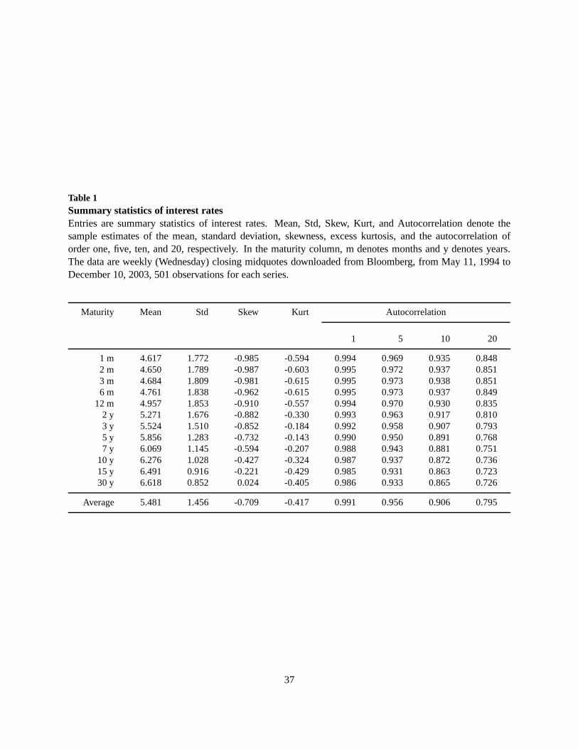
Table 1Summary statistics of interest ratesEntries are summary statistics of interest rates. Mean, Std, Skew, Kurt, and Autocorrelation denote thesample estimates of the mean, standard deviation, skewness, excess kurtosis, and the autocorrelation oforder one, five, ten, and 20, respectively. In the maturity column, m denotes months and y denotes years.The data are weekly (Wednesday) closing midquotes downloaded from Bloomberg, from May 11, 1994 toDecember 10, 2003, 501 observations for each series.

Maturity Mean Std Skew Kurt Autocorrelation

1 5 10 20

1 m 4.617 1.772 -0.985 -0.594 0.994 0.969 0.935 0.8482 m 4.650 1.789 -0.987 -0.603 0.995 0.972 0.937 0.8513 m 4.684 1.809 -0.981 -0.615 0.995 0.973 0.938 0.8516 m 4.761 1.838 -0.962 -0.615 0.995 0.973 0.937 0.849

12 m 4.957 1.853 -0.910 -0.557 0.994 0.970 0.930 0.8352 y 5.271 1.676 -0.882 -0.330 0.993 0.963 0.917 0.8103 y 5.524 1.510 -0.852 -0.184 0.992 0.958 0.907 0.7935 y 5.856 1.283 -0.732 -0.143 0.990 0.950 0.891 0.7687 y 6.069 1.145 -0.594 -0.207 0.988 0.943 0.881 0.751

10 y 6.276 1.028 -0.427 -0.324 0.987 0.937 0.872 0.73615 y 6.491 0.916 -0.221 -0.429 0.985 0.931 0.863 0.72330 y 6.618 0.852 0.024 -0.405 0.986 0.933 0.865 0.726

Average 5.481 1.456 -0.709 -0.417 0.991 0.956 0.906 0.795

37

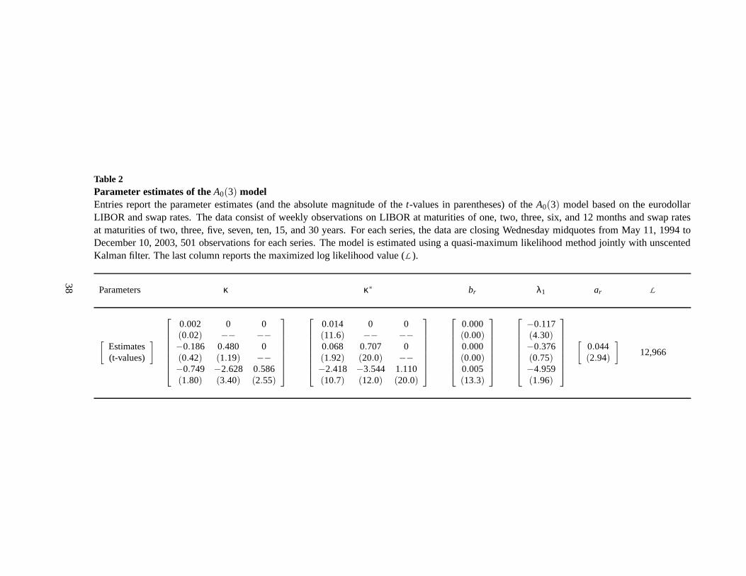
Table 2Parameter estimates of theA0(3) modelEntries report the parameter estimates (and the absolute magnitude of thet-values in parentheses) of theA0(3) model based on the eurodollarLIBOR and swap rates. The data consist of weekly observations on LIBOR at maturities of one, two, three, six, and 12 monthsand swap ratesat maturities of two, three, five, seven, ten, 15, and 30 years. For each series, the data are closing Wednesday midquotes from May 11, 1994 toDecember 10, 2003, 501 observations for each series. The model is estimated using a quasi-maximum likelihood method jointly with unscentedKalman filter. The last column reports the maximized log likelihood value (L ).

Parameters κ κ∗ br λ1 ar L

[

Estimates(t-values)

]

0.002 0 0(0.02) −− −−−0.186 0.480 0(0.42) (1.19) −−−0.749 −2.628 0.586(1.80) (3.40) (2.55)

0.014 0 0(11.6) −− −−0.068 0.707 0(1.92) (20.0) −−−2.418 −3.544 1.110(10.7) (12.0) (20.0)

0.000(0.00)0.000(0.00)0.005(13.3)

−0.117(4.30)−0.376(0.75)−4.959(1.96)

[

0.044(2.94)

]

12,966

38

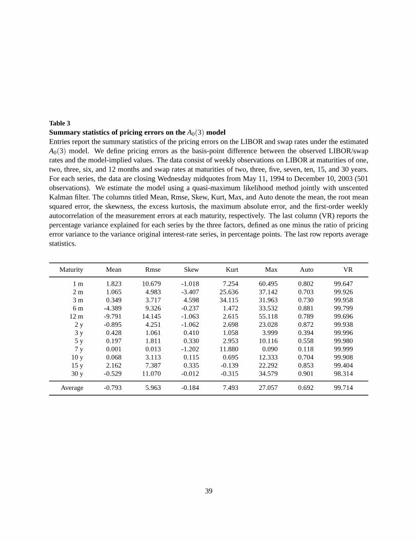
Table 3Summary statistics of pricing errors on theA0(3) modelEntries report the summary statistics of the pricing errorson the LIBOR and swap rates under the estimatedA0(3) model. We define pricing errors as the basis-point difference between the observed LIBOR/swaprates and the model-implied values. The data consist of weekly observations on LIBOR at maturities of one,two, three, six, and 12 months and swap rates at maturities oftwo, three, five, seven, ten, 15, and 30 years.For each series, the data are closing Wednesday midquotes from May 11, 1994 to December 10, 2003 (501observations). We estimate the model using a quasi-maximumlikelihood method jointly with unscentedKalman filter. The columns titled Mean, Rmse, Skew, Kurt, Max, and Auto denote the mean, the root meansquared error, the skewness, the excess kurtosis, the maximum absolute error, and the first-order weeklyautocorrelation of the measurement errors at each maturity, respectively. The last column (VR) reports thepercentage variance explained for each series by the three factors, defined as one minus the ratio of pricingerror variance to the variance original interest-rate series, in percentage points. The last row reports averagestatistics.

Maturity Mean Rmse Skew Kurt Max Auto VR

1 m 1.823 10.679 -1.018 7.254 60.495 0.802 99.6472 m 1.065 4.983 -3.407 25.636 37.142 0.703 99.9263 m 0.349 3.717 4.598 34.115 31.963 0.730 99.9586 m -4.389 9.326 -0.237 1.472 33.532 0.881 99.799

12 m -9.791 14.145 -1.063 2.615 55.118 0.789 99.6962 y -0.895 4.251 -1.062 2.698 23.028 0.872 99.9383 y 0.428 1.061 0.410 1.058 3.999 0.394 99.9965 y 0.197 1.811 0.330 2.953 10.116 0.558 99.9807 y 0.001 0.013 -1.202 11.880 0.090 0.118 99.999

10 y 0.068 3.113 0.115 0.695 12.333 0.704 99.90815 y 2.162 7.387 0.335 -0.139 22.292 0.853 99.40430 y -0.529 11.070 -0.012 -0.315 34.579 0.901 98.314

Average -0.793 5.963 -0.184 7.493 27.057 0.692 99.714

39

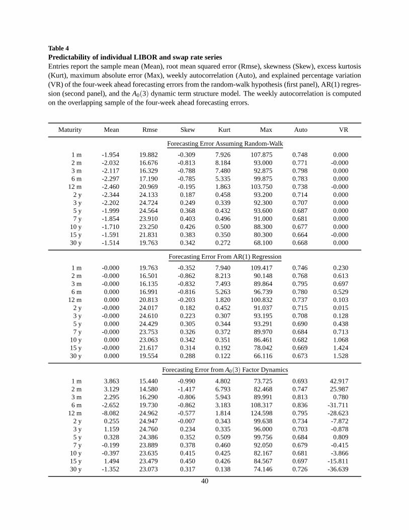
Table 4Predictability of individual LIBOR and swap rate seriesEntries report the sample mean (Mean), root mean squared error (Rmse), skewness (Skew), excess kurtosis(Kurt), maximum absolute error (Max), weekly autocorrelation (Auto), and explained percentage variation(VR) of the four-week ahead forecasting errors from the random-walk hypothesis (first panel), AR(1) regres-sion (second panel), and theA0(3) dynamic term structure model. The weekly autocorrelation is computedon the overlapping sample of the four-week ahead forecasting errors.

Maturity Mean Rmse Skew Kurt Max Auto VR

Forecasting Error Assuming Random-Walk

1 m -1.954 19.882 -0.309 7.926 107.875 0.748 0.0002 m -2.032 16.676 -0.813 8.184 93.000 0.771 -0.0003 m -2.117 16.329 -0.788 7.480 92.875 0.798 0.0006 m -2.297 17.190 -0.785 5.335 99.875 0.783 0.000

12 m -2.460 20.969 -0.195 1.863 103.750 0.738 -0.0002 y -2.344 24.133 0.187 0.458 93.200 0.714 0.0003 y -2.202 24.724 0.249 0.339 92.300 0.707 0.0005 y -1.999 24.564 0.368 0.432 93.600 0.687 0.0007 y -1.854 23.910 0.403 0.496 91.000 0.681 0.000

10 y -1.710 23.250 0.426 0.500 88.300 0.677 0.00015 y -1.591 21.831 0.383 0.350 80.300 0.664 -0.00030 y -1.514 19.763 0.342 0.272 68.100 0.668 0.000

Forecasting Error From AR(1) Regression

1 m -0.000 19.763 -0.352 7.940 109.417 0.746 0.2302 m -0.000 16.501 -0.862 8.213 90.148 0.768 0.6133 m -0.000 16.135 -0.832 7.493 89.864 0.795 0.6976 m 0.000 16.991 -0.816 5.263 96.739 0.780 0.529

12 m 0.000 20.813 -0.203 1.820 100.832 0.737 0.1032 y -0.000 24.017 0.182 0.452 91.037 0.715 0.0153 y -0.000 24.610 0.223 0.307 93.195 0.708 0.1285 y 0.000 24.429 0.305 0.344 93.291 0.690 0.4387 y -0.000 23.753 0.326 0.372 89.970 0.684 0.713

10 y 0.000 23.063 0.342 0.351 86.461 0.682 1.06815 y -0.000 21.617 0.314 0.192 78.042 0.669 1.42430 y 0.000 19.554 0.288 0.122 66.116 0.673 1.528

Forecasting Error fromA0(3) Factor Dynamics

1 m 3.863 15.440 -0.990 4.802 73.725 0.693 42.9172 m 3.129 14.580 -1.417 6.793 82.468 0.747 25.9873 m 2.295 16.290 -0.806 5.943 89.991 0.813 0.7806 m -2.652 19.730 -0.862 3.183 108.317 0.836 -31.711

12 m -8.082 24.962 -0.577 1.814 124.598 0.795 -28.6232 y 0.255 24.947 -0.007 0.343 99.638 0.734 -7.8723 y 1.159 24.760 0.234 0.335 96.000 0.703 -0.8785 y 0.328 24.386 0.352 0.509 99.756 0.684 0.8097 y -0.199 23.889 0.378 0.460 92.050 0.679 -0.415

10 y -0.397 23.635 0.415 0.425 82.167 0.681 -3.86615 y 1.494 23.479 0.450 0.426 84.567 0.697 -15.81130 y -1.352 23.073 0.317 0.138 74.146 0.726 -36.639

40

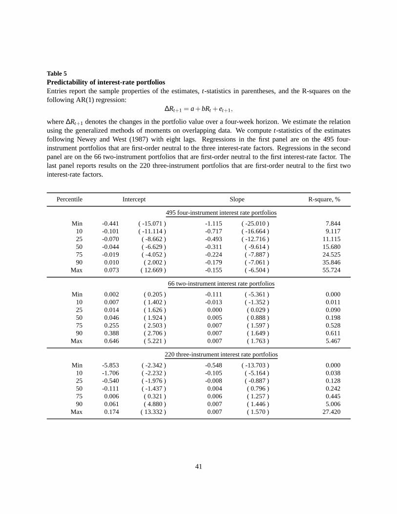
Table 5Predictability of interest-rate portfoliosEntries report the sample properties of the estimates,t-statistics in parentheses, and the R-squares on thefollowing AR(1) regression:

∆Rt+1 = a+bRt +et+1,

where∆Rt+1 denotes the changes in the portfolio value over a four-week horizon. We estimate the relationusing the generalized methods of moments on overlapping data. We computet-statistics of the estimatesfollowing Newey and West (1987) with eight lags. Regressions in the first panel are on the 495 four-instrument portfolios that are first-order neutral to the three interest-rate factors. Regressions in the secondpanel are on the 66 two-instrument portfolios that are first-order neutral to the first interest-rate factor. Thelast panel reports results on the 220 three-instrument portfolios that are first-order neutral to the first twointerest-rate factors.

Percentile Intercept Slope R-square, %

495 four-instrument interest rate portfolios

Min -0.441 ( -15.071 ) -1.115 ( -25.010 ) 7.84410 -0.101 ( -11.114 ) -0.717 ( -16.664 ) 9.11725 -0.070 ( -8.662 ) -0.493 ( -12.716 ) 11.11550 -0.044 ( -6.629 ) -0.311 ( -9.614 ) 15.68075 -0.019 ( -4.052 ) -0.224 ( -7.887 ) 24.52590 0.010 ( 2.002 ) -0.179 ( -7.061 ) 35.846

Max 0.073 ( 12.669 ) -0.155 ( -6.504 ) 55.724

66 two-instrument interest rate portfolios

Min 0.002 ( 0.205 ) -0.111 ( -5.361 ) 0.00010 0.007 ( 1.402 ) -0.013 ( -1.352 ) 0.01125 0.014 ( 1.626 ) 0.000 ( 0.029 ) 0.09050 0.046 ( 1.924 ) 0.005 ( 0.888 ) 0.19875 0.255 ( 2.503 ) 0.007 ( 1.597 ) 0.52890 0.388 ( 2.706 ) 0.007 ( 1.649 ) 0.611

Max 0.646 ( 5.221 ) 0.007 ( 1.763 ) 5.467

220 three-instrument interest rate portfolios

Min -5.853 ( -2.342 ) -0.548 ( -13.703 ) 0.00010 -1.706 ( -2.232 ) -0.105 ( -5.164 ) 0.03825 -0.540 ( -1.976 ) -0.008 ( -0.887 ) 0.12850 -0.111 ( -1.437 ) 0.004 ( 0.796 ) 0.24275 0.006 ( 0.321 ) 0.006 ( 1.257 ) 0.44590 0.061 ( 4.880 ) 0.007 ( 1.446 ) 5.006

Max 0.174 ( 13.332 ) 0.007 ( 1.570 ) 27.420

41

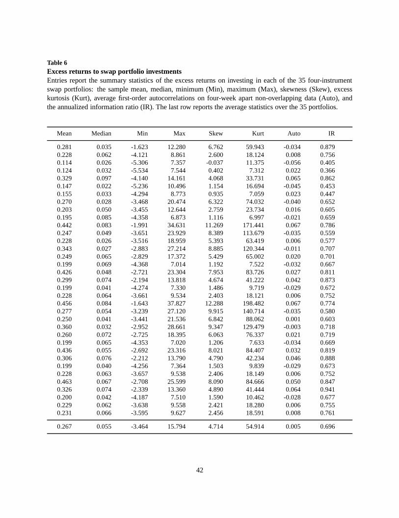
Table 6Excess returns to swap portfolio investmentsEntries report the summary statistics of the excess returnson investing in each of the 35 four-instrumentswap portfolios: the sample mean, median, minimum (Min), maximum (Max), skewness (Skew), excesskurtosis (Kurt), average first-order autocorrelations on four-week apart non-overlapping data (Auto), andthe annualized information ratio (IR). The last row reportsthe average statistics over the 35 portfolios.

Mean Median Min Max Skew Kurt Auto IR

0.281 0.035 -1.623 12.280 6.762 59.943 -0.034 0.8790.228 0.062 -4.121 8.861 2.600 18.124 0.008 0.7560.114 0.026 -5.306 7.357 -0.037 11.375 -0.056 0.4050.124 0.032 -5.534 7.544 0.402 7.312 0.022 0.3660.329 0.097 -4.140 14.161 4.068 33.731 0.065 0.8620.147 0.022 -5.236 10.496 1.154 16.694 -0.045 0.4530.155 0.033 -4.294 8.773 0.935 7.059 0.023 0.4470.270 0.028 -3.468 20.474 6.322 74.032 -0.040 0.6520.203 0.050 -3.455 12.644 2.759 23.734 0.016 0.6050.195 0.085 -4.358 6.873 1.116 6.997 -0.021 0.6590.442 0.083 -1.991 34.631 11.269 171.441 0.067 0.7860.247 0.049 -3.651 23.929 8.389 113.679 -0.035 0.5590.228 0.026 -3.516 18.959 5.393 63.419 0.006 0.5770.343 0.027 -2.883 27.214 8.885 120.344 -0.011 0.7070.249 0.065 -2.829 17.372 5.429 65.002 0.020 0.7010.199 0.069 -4.368 7.014 1.192 7.522 -0.032 0.6670.426 0.048 -2.721 23.304 7.953 83.726 0.027 0.8110.299 0.074 -2.194 13.818 4.674 41.222 0.042 0.8730.199 0.041 -4.274 7.330 1.486 9.719 -0.029 0.6720.228 0.064 -3.661 9.534 2.403 18.121 0.006 0.7520.456 0.084 -1.643 37.827 12.288 198.482 0.067 0.7740.277 0.054 -3.239 27.120 9.915 140.714 -0.035 0.5800.250 0.041 -3.441 21.536 6.842 88.062 0.001 0.6030.360 0.032 -2.952 28.661 9.347 129.479 -0.003 0.7180.260 0.072 -2.725 18.395 6.063 76.337 0.021 0.7190.199 0.065 -4.353 7.020 1.206 7.633 -0.034 0.6690.436 0.055 -2.692 23.316 8.021 84.407 0.032 0.8190.306 0.076 -2.212 13.790 4.790 42.234 0.046 0.8880.199 0.040 -4.256 7.364 1.503 9.839 -0.029 0.6730.228 0.063 -3.657 9.538 2.406 18.149 0.006 0.7520.463 0.067 -2.708 25.599 8.090 84.666 0.050 0.8470.326 0.074 -2.339 13.360 4.890 41.444 0.064 0.9410.200 0.042 -4.187 7.510 1.590 10.462 -0.028 0.6770.229 0.062 -3.638 9.558 2.421 18.280 0.006 0.7550.231 0.066 -3.595 9.627 2.456 18.591 0.008 0.761

0.267 0.055 -3.464 15.794 4.714 54.914 0.005 0.696

42

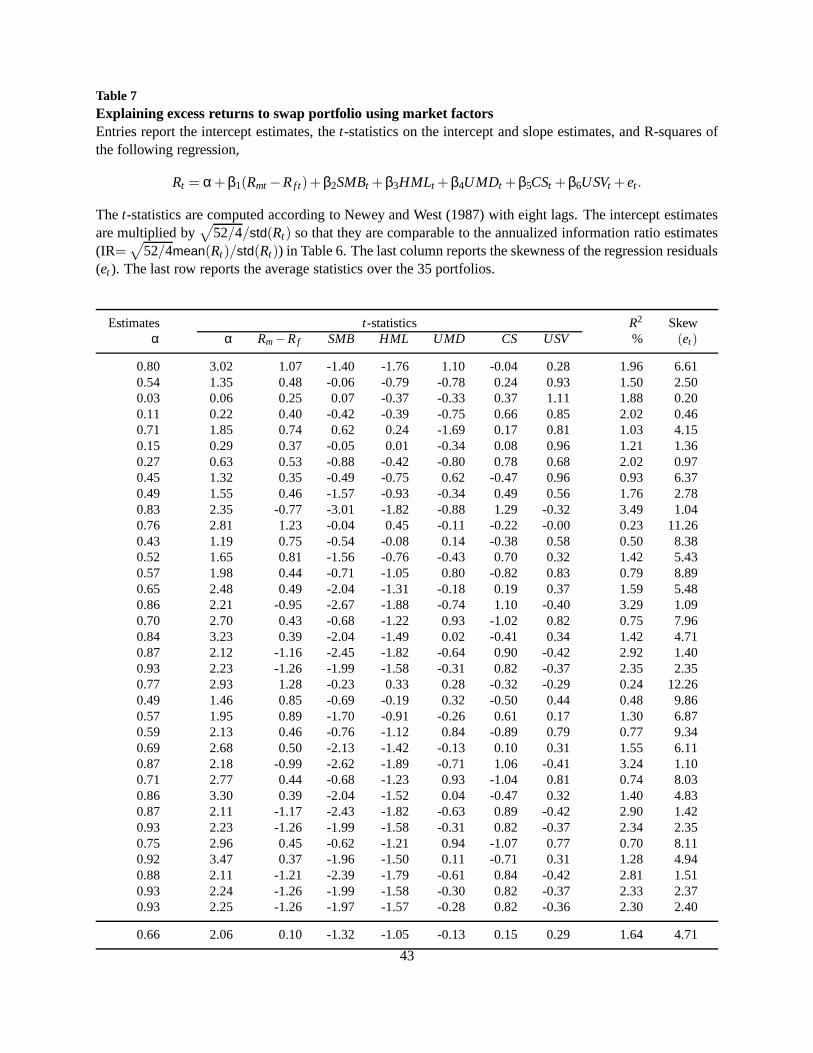
Table 7Explaining excess returns to swap portfolio using market factorsEntries report the intercept estimates, thet-statistics on the intercept and slope estimates, and R-squares ofthe following regression,

Rt = α+ β1(Rmt−Rf t)+ β2SMBt + β3HMLt + β4UMDt + β5CSt + β6USVt +et .

Thet-statistics are computed according to Newey and West (1987)with eight lags. The intercept estimatesare multiplied by

√

52/4/std(Rt) so that they are comparable to the annualized information ratio estimates(IR=

√

52/4mean(Rt)/std(Rt)) in Table 6. The last column reports the skewness of the regression residuals(et ). The last row reports the average statistics over the 35 portfolios.

Estimates t-statistics R2 Skewα α Rm−Rf SMB HML UMD CS USV % (et)

0.80 3.02 1.07 -1.40 -1.76 1.10 -0.04 0.28 1.96 6.610.54 1.35 0.48 -0.06 -0.79 -0.78 0.24 0.93 1.50 2.500.03 0.06 0.25 0.07 -0.37 -0.33 0.37 1.11 1.88 0.200.11 0.22 0.40 -0.42 -0.39 -0.75 0.66 0.85 2.02 0.460.71 1.85 0.74 0.62 0.24 -1.69 0.17 0.81 1.03 4.150.15 0.29 0.37 -0.05 0.01 -0.34 0.08 0.96 1.21 1.360.27 0.63 0.53 -0.88 -0.42 -0.80 0.78 0.68 2.02 0.970.45 1.32 0.35 -0.49 -0.75 0.62 -0.47 0.96 0.93 6.370.49 1.55 0.46 -1.57 -0.93 -0.34 0.49 0.56 1.76 2.780.83 2.35 -0.77 -3.01 -1.82 -0.88 1.29 -0.32 3.49 1.040.76 2.81 1.23 -0.04 0.45 -0.11 -0.22 -0.00 0.23 11.260.43 1.19 0.75 -0.54 -0.08 0.14 -0.38 0.58 0.50 8.380.52 1.65 0.81 -1.56 -0.76 -0.43 0.70 0.32 1.42 5.430.57 1.98 0.44 -0.71 -1.05 0.80 -0.82 0.83 0.79 8.890.65 2.48 0.49 -2.04 -1.31 -0.18 0.19 0.37 1.59 5.480.86 2.21 -0.95 -2.67 -1.88 -0.74 1.10 -0.40 3.29 1.090.70 2.70 0.43 -0.68 -1.22 0.93 -1.02 0.82 0.75 7.960.84 3.23 0.39 -2.04 -1.49 0.02 -0.41 0.34 1.42 4.710.87 2.12 -1.16 -2.45 -1.82 -0.64 0.90 -0.42 2.92 1.400.93 2.23 -1.26 -1.99 -1.58 -0.31 0.82 -0.37 2.35 2.350.77 2.93 1.28 -0.23 0.33 0.28 -0.32 -0.29 0.24 12.260.49 1.46 0.85 -0.69 -0.19 0.32 -0.50 0.44 0.48 9.860.57 1.95 0.89 -1.70 -0.91 -0.26 0.61 0.17 1.30 6.870.59 2.13 0.46 -0.76 -1.12 0.84 -0.89 0.79 0.77 9.340.69 2.68 0.50 -2.13 -1.42 -0.13 0.10 0.31 1.55 6.110.87 2.18 -0.99 -2.62 -1.89 -0.71 1.06 -0.41 3.24 1.100.71 2.77 0.44 -0.68 -1.23 0.93 -1.04 0.81 0.74 8.030.86 3.30 0.39 -2.04 -1.52 0.04 -0.47 0.32 1.40 4.830.87 2.11 -1.17 -2.43 -1.82 -0.63 0.89 -0.42 2.90 1.420.93 2.23 -1.26 -1.99 -1.58 -0.31 0.82 -0.37 2.34 2.350.75 2.96 0.45 -0.62 -1.21 0.94 -1.07 0.77 0.70 8.110.92 3.47 0.37 -1.96 -1.50 0.11 -0.71 0.31 1.28 4.940.88 2.11 -1.21 -2.39 -1.79 -0.61 0.84 -0.42 2.81 1.510.93 2.24 -1.26 -1.99 -1.58 -0.30 0.82 -0.37 2.33 2.370.93 2.25 -1.26 -1.97 -1.57 -0.28 0.82 -0.36 2.30 2.40

0.66 2.06 0.10 -1.32 -1.05 -0.13 0.15 0.29 1.64 4.71

43

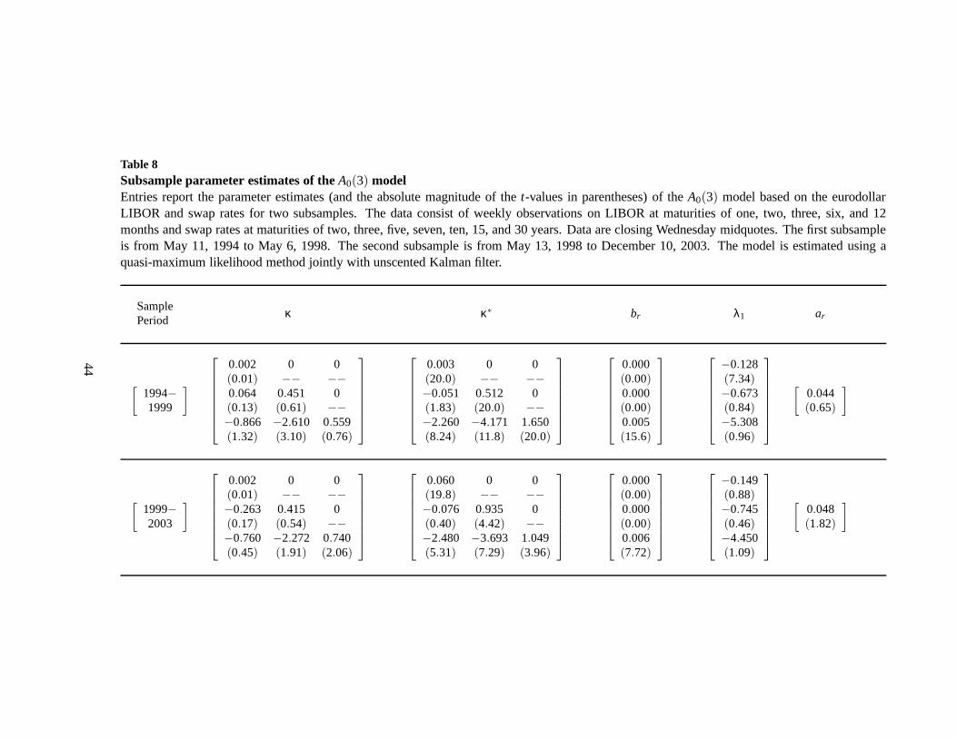
Table 8Subsample parameter estimates of theA0(3) modelEntries report the parameter estimates (and the absolute magnitude of thet-values in parentheses) of theA0(3) model based on the eurodollarLIBOR and swap rates for two subsamples. The data consist of weekly observations on LIBOR at maturities of one, two, three, six, and 12months and swap rates at maturities of two, three, five, seven, ten, 15, and 30 years. Data are closing Wednesday midquotes. The first subsampleis from May 11, 1994 to May 6, 1998. The second subsample is from May 13, 1998 to December 10, 2003. The model is estimated using aquasi-maximum likelihood method jointly with unscented Kalman filter.

SamplePeriod

κ κ∗ br λ1 ar

[

1994−1999

]

0.002 0 0(0.01) −− −−0.064 0.451 0(0.13) (0.61) −−−0.866 −2.610 0.559(1.32) (3.10) (0.76)

0.003 0 0(20.0) −− −−−0.051 0.512 0(1.83) (20.0) −−−2.260 −4.171 1.650(8.24) (11.8) (20.0)

0.000(0.00)0.000(0.00)0.005(15.6)

−0.128(7.34)−0.673(0.84)−5.308(0.96)

[

0.044(0.65)

]

[

1999−2003

]

0.002 0 0(0.01) −− −−−0.263 0.415 0(0.17) (0.54) −−−0.760 −2.272 0.740(0.45) (1.91) (2.06)

0.060 0 0(19.8) −− −−−0.076 0.935 0(0.40) (4.42) −−−2.480 −3.693 1.049(5.31) (7.29) (3.96)

0.000(0.00)0.000(0.00)0.006(7.72)

−0.149(0.88)−0.745(0.46)−4.450(1.09)

[

0.048(1.82)

]

44

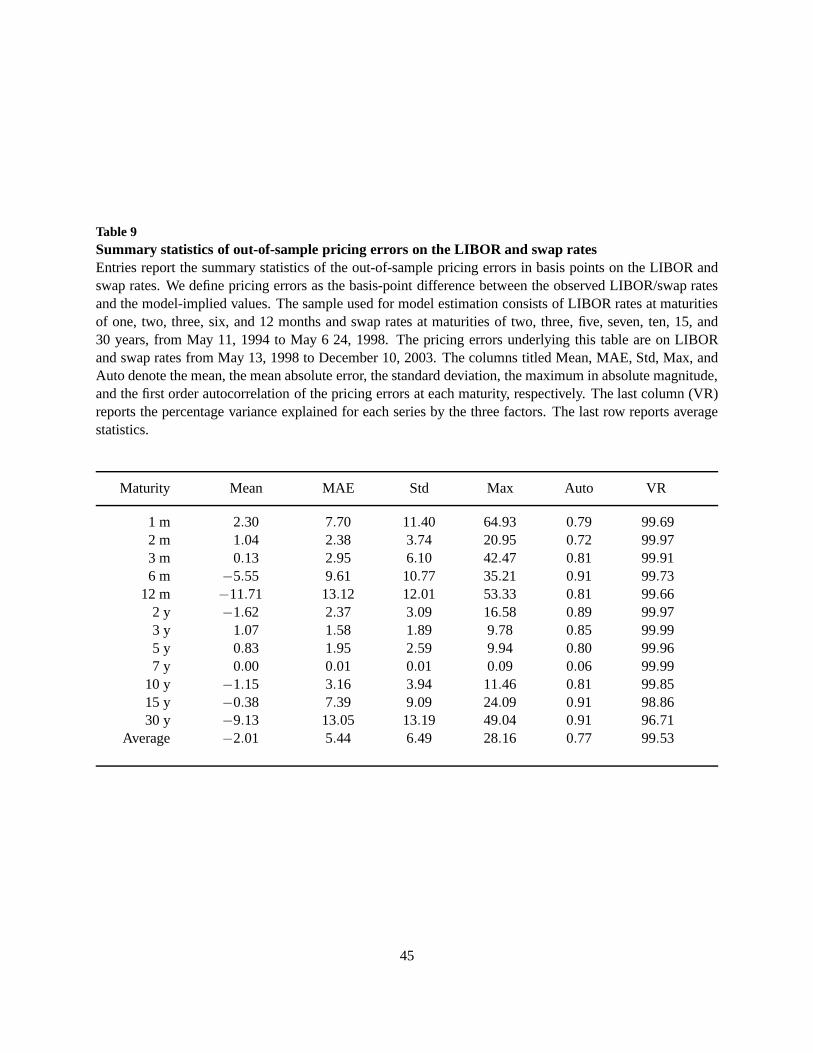
Table 9Summary statistics of out-of-sample pricing errors on the LIBOR and swap ratesEntries report the summary statistics of the out-of-samplepricing errors in basis points on the LIBOR andswap rates. We define pricing errors as the basis-point difference between the observed LIBOR/swap ratesand the model-implied values. The sample used for model estimation consists of LIBOR rates at maturitiesof one, two, three, six, and 12 months and swap rates at maturities of two, three, five, seven, ten, 15, and30 years, from May 11, 1994 to May 6 24, 1998. The pricing errors underlying this table are on LIBORand swap rates from May 13, 1998 to December 10, 2003. The columns titled Mean, MAE, Std, Max, andAuto denote the mean, the mean absolute error, the standard deviation, the maximum in absolute magnitude,and the first order autocorrelation of the pricing errors at each maturity, respectively. The last column (VR)reports the percentage variance explained for each series by the three factors. The last row reports averagestatistics.

Maturity Mean MAE Std Max Auto VR

1 m 2.30 7.70 11.40 64.93 0.79 99.692 m 1.04 2.38 3.74 20.95 0.72 99.973 m 0.13 2.95 6.10 42.47 0.81 99.916 m −5.55 9.61 10.77 35.21 0.91 99.73

12 m −11.71 13.12 12.01 53.33 0.81 99.662 y −1.62 2.37 3.09 16.58 0.89 99.973 y 1.07 1.58 1.89 9.78 0.85 99.995 y 0.83 1.95 2.59 9.94 0.80 99.967 y 0.00 0.01 0.01 0.09 0.06 99.99

10 y −1.15 3.16 3.94 11.46 0.81 99.8515 y −0.38 7.39 9.09 24.09 0.91 98.8630 y −9.13 13.05 13.19 49.04 0.91 96.71

Average −2.01 5.44 6.49 28.16 0.77 99.53

45

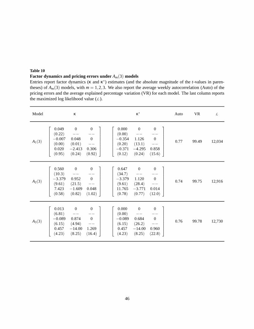
Table 10Factor dynamics and pricing errors under Am(3) modelsEntries report factor dynamics (κ andκ∗) estimates (and the absolute magnitude of thet-values in paren-theses) ofAm(3) models, withm= 1,2,3. We also report the average weekly autocorrelation (Auto)of thepricing errors and the average explained percentage variation (VR) for each model. The last column reportsthe maximized log likelihood value (L ).

Model κ κ∗ Auto VR L

A1(3)

0.049 0 0(0.22) −− −−−0.007 0.048 0(0.00) (0.01) −−0.020 −2.413 0.306(0.95) (0.24) (0.92)

0.000 0 0(0.00) −− −−−0.354 1.126 0(0.20) (13.1) −−−0.371 −4.295 0.858(0.12) (0.24) (15.6)

0.77 99.49 12,034

A2(3)

0.560 0 0(10.3) −− −−−3.379 0.952 0(9.61) (21.5) −−7.423 −1.609 0.048(0.58) (0.82) (1.02)

0.647 0 0(34.7) −− −−−3.379 1.120 0(9.61) (28.4) −−11.765 −3.771 0.014(0.78) (0.77) (12.0)

0.74 99.75 12,916

A3(3)

0.013 0 0(6.81) −− −−−0.089 0.874 0(6.15) (4.94) −−0.457 −14.00 1.269(4.23) (8.25) (16.4)

0.000 0 0(0.00) −− −−−0.089 0.684 0(6.15) (26.2) −−0.457 −14.00 0.960(4.23) (8.25) (22.8)

0.76 99.78 12,730

46

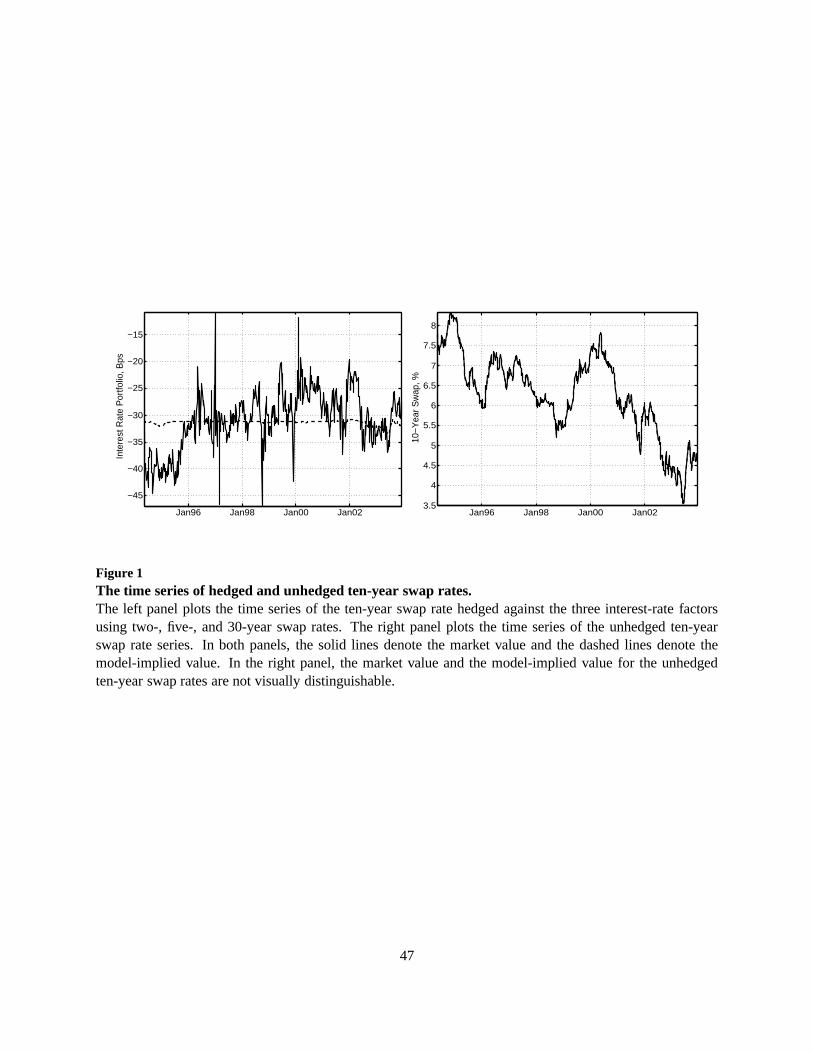
Jan96 Jan98 Jan00 Jan02

−45

−40

−35

−30

−25

−20

−15

Inte

rest

Rat

e P

ortfo

lio, B

ps

Jan96 Jan98 Jan00 Jan023.5

4

4.5

5

5.5

6

6.5

7

7.5

8

10−Y

ear

Sw

ap, %

Figure 1The time series of hedged and unhedged ten-year swap rates.The left panel plots the time series of the ten-year swap ratehedged against the three interest-rate factorsusing two-, five-, and 30-year swap rates. The right panel plots the time series of the unhedged ten-yearswap rate series. In both panels, the solid lines denote the market value and the dashed lines denote themodel-implied value. In the right panel, the market value and the model-implied value for the unhedgedten-year swap rates are not visually distinguishable.

47

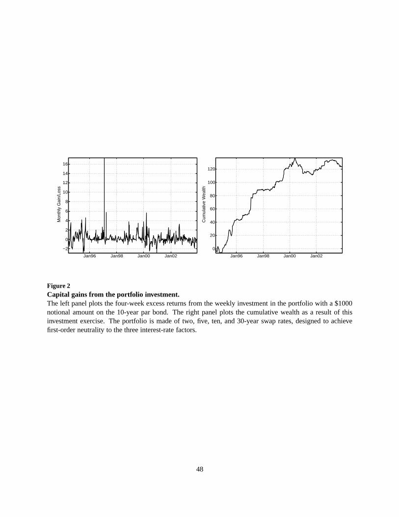
Jan96 Jan98 Jan00 Jan02

−2

0

2

4

6

8

10

12

14

16

Mon

thly

Gai

n/Lo

ss

Jan96 Jan98 Jan00 Jan02

0

20

40

60

80

100

120

Cum

ulat

ive

Wea

lth

Figure 2Capital gains from the portfolio investment.The left panel plots the four-week excess returns from the weekly investment in the portfolio with a $1000notional amount on the 10-year par bond. The right panel plots the cumulative wealth as a result of thisinvestment exercise. The portfolio is made of two, five, ten,and 30-year swap rates, designed to achievefirst-order neutrality to the three interest-rate factors.

48

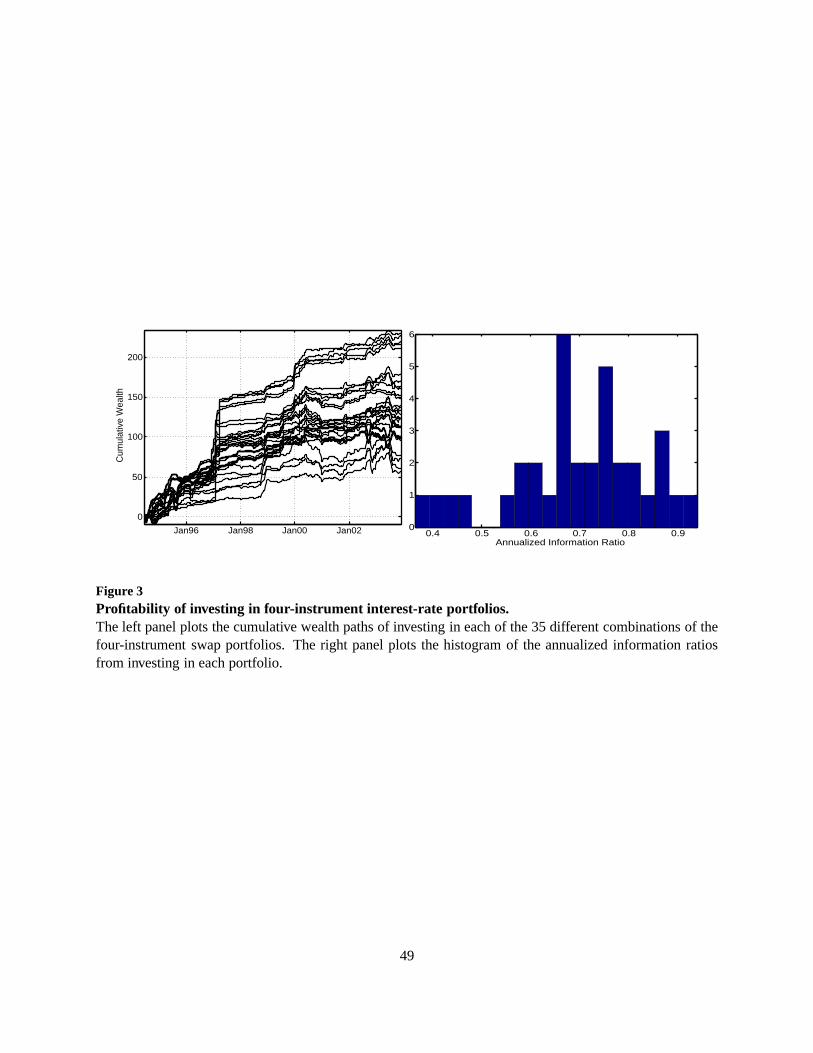
Jan96 Jan98 Jan00 Jan02

0

50

100

150

200

Cum

ulat

ive

Wea

lth

0.4 0.5 0.6 0.7 0.8 0.90

1

2

3

4

5

6

Annualized Information Ratio

Figure 3Profitability of investing in four-instrument interest-ra te portfolios.The left panel plots the cumulative wealth paths of investing in each of the 35 different combinations of thefour-instrument swap portfolios. The right panel plots thehistogram of the annualized information ratiosfrom investing in each portfolio.

49

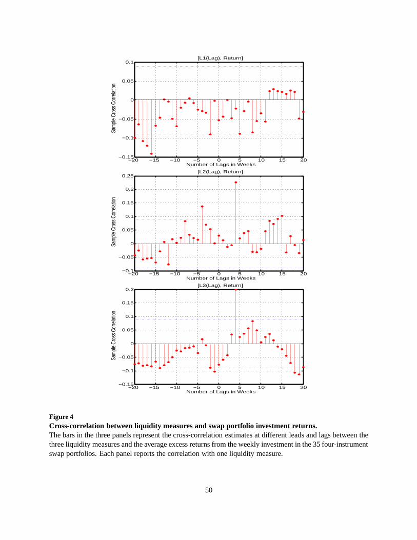
−20 −15 −10 −5 0 5 10 15 20−0.15

−0.1

−0.05

0

0.05

0.1

Number of Lags in Weeks

Sam

ple C

ross

Cor

relat

ion

[L1(Lag), Return]

−20 −15 −10 −5 0 5 10 15 20−0.1

−0.05

0

0.05

0.1

0.15

0.2

0.25

Number of Lags in Weeks

Sam

ple C

ross

Cor

relat

ion

[L2(Lag), Return]

−20 −15 −10 −5 0 5 10 15 20−0.15

−0.1

−0.05

0

0.05

0.1

0.15

0.2

Number of Lags in Weeks

Sam

ple C

ross

Cor

relat

ion

[L3(Lag), Return]

Figure 4Cross-correlation between liquidity measures and swap portfolio investment returns.The bars in the three panels represent the cross-correlation estimates at different leads and lags between thethree liquidity measures and the average excess returns from the weekly investment in the 35 four-instrumentswap portfolios. Each panel reports the correlation with one liquidity measure.

50

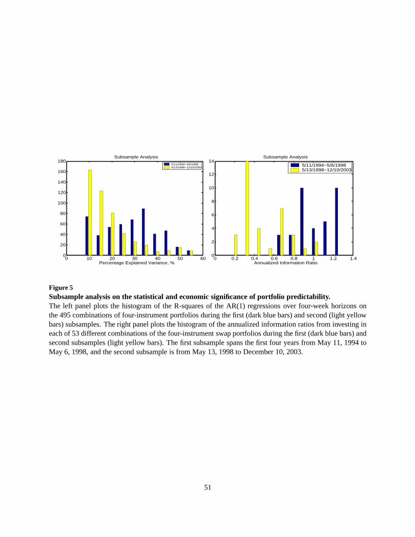
0 10 20 30 40 50 600

20

40

60

80

100

120

140

160

180

Percentage Explained Variance, %

Subsample Analysis

5/11/1994−5/6/19985/13/1998−12/10/2003

0 0.2 0.4 0.6 0.8 1 1.2 1.40

2

4

6

8

10

12

14

Annualized Information Ratio

Subsample Analysis

5/11/1994−5/6/19985/13/1998−12/10/2003

Figure 5Subsample analysis on the statistical and economic significance of portfolio predictability.The left panel plots the histogram of the R-squares of the AR(1) regressions over four-week horizons onthe 495 combinations of four-instrument portfolios duringthe first (dark blue bars) and second (light yellowbars) subsamples. The right panel plots the histogram of theannualized information ratios from investing ineach of 53 different combinations of the four-instrument swap portfolios during the first (dark blue bars) andsecond subsamples (light yellow bars). The first subsample spans the first four years from May 11, 1994 toMay 6, 1998, and the second subsample is from May 13, 1998 to December 10, 2003.

51

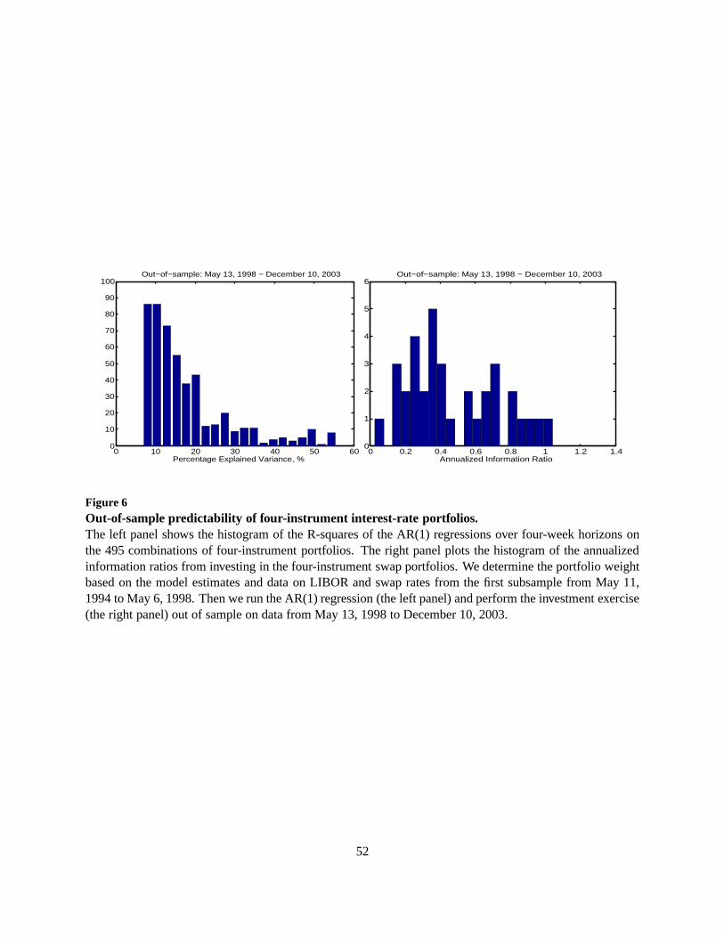
0 10 20 30 40 50 600

10

20

30

40

50

60

70

80

90

100

Percentage Explained Variance, %

Out−of−sample: May 13, 1998 − December 10, 2003

0 0.2 0.4 0.6 0.8 1 1.2 1.40

1

2

3

4

5

6

Annualized Information Ratio

Out−of−sample: May 13, 1998 − December 10, 2003

Figure 6Out-of-sample predictability of four-instrument interest-rate portfolios.The left panel shows the histogram of the R-squares of the AR(1) regressions over four-week horizons onthe 495 combinations of four-instrument portfolios. The right panel plots the histogram of the annualizedinformation ratios from investing in the four-instrument swap portfolios. We determine the portfolio weightbased on the model estimates and data on LIBOR and swap rates from the first subsample from May 11,1994 to May 6, 1998. Then we run the AR(1) regression (the leftpanel) and perform the investment exercise(the right panel) out of sample on data from May 13, 1998 to December 10, 2003.

52

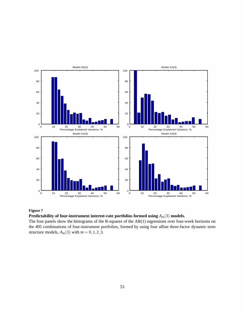
0 10 20 30 40 50 600

20

40

60

80

100

Percentage Explained Variance, %

Model A0(3)

0 10 20 30 40 50 600

20

40

60

80

100

Percentage Explained Variance, %

Model A1(3)

0 10 20 30 40 50 600

20

40

60

80

100

Percentage Explained Variance, %

Model A2(3)

0 10 20 30 40 50 600

20

40

60

80

100

Percentage Explained Variance, %

Model A3(3)

Figure 7Predictability of four-instrument interest-rate portfol ios formed usingAm(3) models.The four panels show the histograms of the R-squares of the AR(1) regressions over four-week horizons onthe 495 combinations of four-instrument portfolios, formed by using four affine three-factor dynamic termstructure models,Am(3) with m= 0,1,2,3.

53