YV - Query Processing and Optimization 369 Κεφάλαιο 9 Επεξεργασία και Βελτιστοποίηση Ερωτήσεων σε Σχεσιακές Βάσεις Δεδομένων

YV - Query Processing and Optimization 1

Κεφάλαιο 9

Επεξεργασία και Βελτιστοποίηση Ερωτήσεων σε Σχεσιακές Βάσεις

Δεδομένων


Query Processing and Optimization

Architecture of the Query Processor in a DBMS Query Processing Implementation of Relational Operators (join,

select, project, aggregates, etc.)– Use of Indices– Buffering

Query Optimization– Plans– Nested Queries


Architecture of the QUERY PROCESSOR

TERMINAL MONITOR

QUERY LANGUAGE COMPILER

QUERY OPTIMIZER

CODE GENERATOR / INTERPRETER

ACCESS METHOD

FILE SYSTEM

Query Language

Internal Form (e.g., Relational Algebra)

Internal Form (e.g., Relational Algebra)

Record-at-a-time callsembedded in a program

Page-at-a-time accessto files

Select e.namefrom empl e, dept dwhere e.dno = d.dno and d.floor=3

ÐName ( (e d)

(plans)

manipulate records

manipulat pages

floor=3

ÐName ( e ( d)

floor=3


Query Processing in a DBMS

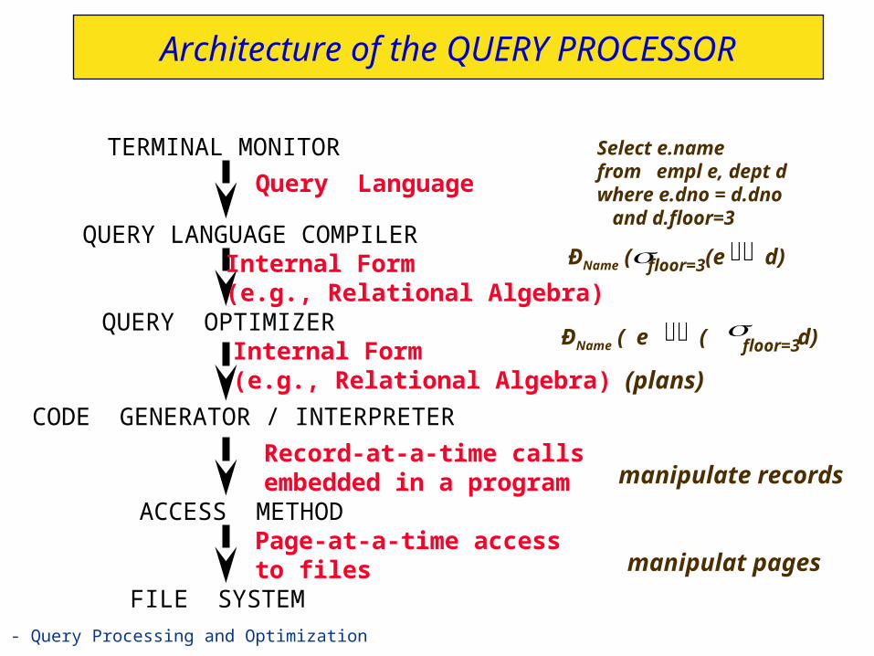
The Query Language Compiler translates the query into an internal form, usually a relational algebra expression

The Query Optimizer examines all the equivalent algebraic expressions (plans) and chooses the one that is estimated as cheapest– Uses estimates of sizes, usage and contents of the

relations (kept in catalogs and updated dynamically)– Uses the knowledge of the Cost for relational database

operations (how the joins are implemented, etc.)


Query Processing in a DBMS -- (b)

The Code Generator implements the access plan generated by the Optimizer

The Access Methods support commands to access records of a file (one at a time). FUNCTIONS of an access method are:– Record Layout on Pages– Field Layout in Records– Data Compression– Indexing Records by Field Values


Query Processing in a DBMS -- (c)

The File System supports page-at-a-time access to files

FUNCTIONS of the File System are:– Partitioning of the file into disks– Managing Free Space on Disk– Issuing Hardware I/O commands– Managing Main Memory Buffers


Relational Operations -- Implementation

We will consider how to implement:– Selection ( ) Selects a subset of rows from relation.– Projection ( ) Deletes unwanted columns from

relation.– Join ( ) Allows us to combine two relations.– Set-difference ( ) Tuples in reln. 1, but not in reln. 2.– Union ( ) Tuples in reln. 1 and in reln. 2.– Aggregation (SUM, MIN, etc.) and GROUP BY

Since each op returns a relation, ops can be composed! After we cover the operations, we will discuss how to optimize queries formed by composing them.


Schema for Examples

Similar to old schema; rname added for variations.

Reserves:– Each tuple is 40 bytes long, 100 tuples per page,

1000 pages. Sailors:

– Each tuple is 50 bytes long, 80 tuples per page, 500 pages.

Sailors (sid: integer, sname: string, rating: integer, age: real)Reserves (sid: integer, bid: integer, day: dates, rname: string)


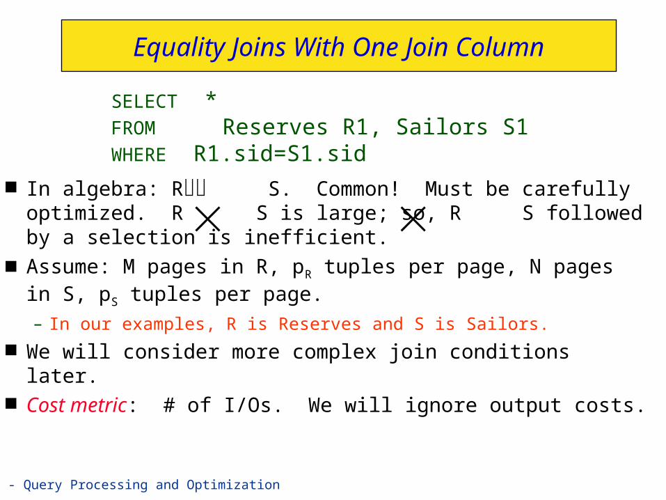
Equality Joins With One Join Column

In algebra: R S. Common! Must be carefully optimized. R S is large; so, R S followed by a selection is inefficient.

Assume: M pages in R, pR tuples per page, N pages in S, pS tuples per page.– In our examples, R is Reserves and S is Sailors.

We will consider more complex join conditions later. Cost metric: # of I/Os. We will ignore output costs.

SELECT *FROM Reserves R1, Sailors S1WHERE R1.sid=S1.sid


Simple Nested Loops Join

For each tuple in the outer relation R, we scan the entire inner relation S. – Cost: M + pR * M * N = 1000 + 100*1000*500 I/Os.

Page-oriented Nested Loops join: For each page of R, get each page of S, and write out matching pairs of tuples <r, s>, where r is in R-page and S is in S-page.– Cost: M + M*N = 1000 + 1000*500– If smaller relation (S) is outer, cost = 500 + 500*1000

foreach tuple r in R doforeach tuple s in S do

if ri == sj then add <r, s> to result


Index Nested Loops Join

If there is an index on the join column of one relation (say S), can make it the inner and exploit the index.– Cost: M + ( (M*pR) * cost of finding matching S tuples)

For each R tuple, cost of probing S index is about 1.2 for hash index, 2-4 for B+ tree. Cost of then finding S tuples (assuming Alt. (2) or (3) for data entries) depends on clustering.– Clustered index: 1 I/O (typical), unclustered: upto 1 I/O

per matching S tuple.

foreach tuple r in R doforeach tuple s in S where ri == sj do

add <r, s> to result


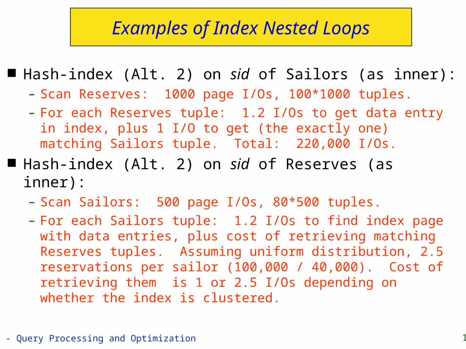
Examples of Index Nested Loops

Hash-index (Alt. 2) on sid of Sailors (as inner):– Scan Reserves: 1000 page I/Os, 100*1000 tuples.– For each Reserves tuple: 1.2 I/Os to get data entry in

index, plus 1 I/O to get (the exactly one) matching Sailors tuple. Total: 220,000 I/Os.

Hash-index (Alt. 2) on sid of Reserves (as inner):– Scan Sailors: 500 page I/Os, 80*500 tuples.– For each Sailors tuple: 1.2 I/Os to find index page with

data entries, plus cost of retrieving matching Reserves tuples. Assuming uniform distribution, 2.5 reservations per sailor (100,000 / 40,000). Cost of retrieving them is 1 or 2.5 I/Os depending on whether the index is clustered.


Block Nested Loops Join

Use one page as an input buffer for scanning the inner S, one page as the output buffer, and use all remaining pages to hold ``block’’ of outer R.– For each matching tuple r in R-block, s in S-page, add

<r, s> to result. Then read next R-block, scan S, etc.

. . .

. . .

R & SHash table for block of R

(k < B-1 pages)

Input buffer for S Output buffer

. . .

Join Result


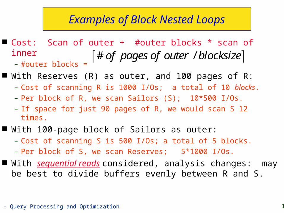
Examples of Block Nested Loops

Cost: Scan of outer + #outer blocks * scan of inner– #outer blocks =

With Reserves (R) as outer, and 100 pages of R:– Cost of scanning R is 1000 I/Os; a total of 10 blocks.– Per block of R, we scan Sailors (S); 10*500 I/Os.– If space for just 90 pages of R, we would scan S 12 times.

With 100-page block of Sailors as outer:– Cost of scanning S is 500 I/Os; a total of 5 blocks.– Per block of S, we scan Reserves; 5*1000 I/Os.

With sequential reads considered, analysis changes: may be best to divide buffers evenly between R and S.

# /of pages of outer blocksize


Sort-Merge Join (R S)

Sort R and S on the join column, then scan them to do a ``merge’’ (on join col.), and output result tuples.– Advance scan of R until current R-tuple >= current S

tuple, then advance scan of S until current S-tuple >= current R tuple; do this until current R tuple = current S tuple.

– At this point, all R tuples with same value in Ri (current R group) and all S tuples with same value in Sj (current S group) match; output <r, s> for all pairs of such tuples.

– Then resume scanning R and S. R is scanned once; each S group is scanned once per

matching R tuple. (Multiple scans of an S group are likely to find needed pages in buffer.)

i=j


Example of Sort-Merge Join

Cost: M log M + N log N + (M+N)– The cost of scanning, M+N, could be M*N (very unlikely!)

With 35, 100 or 300 buffer pages, both Reserves and Sailors can be sorted in 2 passes; total join cost: 7500.

sid sname rating age22 dustin 7 45.028 yuppy 9 35.031 lubber 8 55.544 guppy 5 35.058 rusty 10 35.0

sid bid day rname

28 103 12/4/96 guppy28 103 11/3/96 yuppy31 101 10/10/96 dustin31 102 10/12/96 lubber31 101 10/11/96 lubber58 103 11/12/96 dustin

(BNL cost: 2500 to 15000 I/Os)


Refinement of Sort-Merge Join

We can combine the merging phases in the sorting of R and S with the merging required for the join.– With B > , where L is the size of the larger relation,

using the sorting refinement that produces runs of length 2B in Pass 0, #runs of each relation is < B/2.

– Allocate 1 page per run of each relation, and `merge’ while checking the join condition.

– Cost: read+write each relation in Pass 0 + read each relation in (only) merging pass (+ writing of result tuples).

– In example, cost goes down from 7500 to 4500 I/Os. In practice, cost of sort-merge join, like the cost of

external sorting, is linear.

L


Hash-Join

Partition both relations using hash fn h: R tuples in partition i will only match S tuples in partition i.

Read in a partition of R, hash it using h2 (<> h!). Scan matching partition of S, search for matches.

Partitionsof R & S

Input bufferfor Si

Hash table for partitionRi (k < B-1 pages)

B main memory buffersDisk

Output buffer

Disk

Join Result

hashfnh2

h2

B main memory buffers DiskDisk

Original Relation OUTPUT

2INPUT

1

hashfunction

h B-1

Partitions

1

2

B-1

. . .


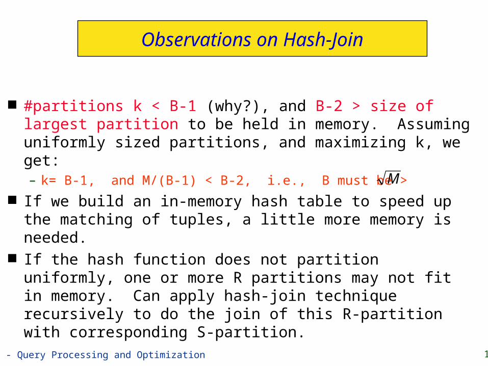
Observations on Hash-Join

#partitions k < B-1 (why?), and B-2 > size of largest partition to be held in memory. Assuming uniformly sized partitions, and maximizing k, we get:– k= B-1, and M/(B-1) < B-2, i.e., B must be >

If we build an in-memory hash table to speed up the matching of tuples, a little more memory is needed.

If the hash function does not partition uniformly, one or more R partitions may not fit in memory. Can apply hash-join technique recursively to do the join of this R-partition with corresponding S-partition.

M


Cost of Hash-Join

In partitioning phase, read+write both relns; 2(M+N). In matching phase, read both relns; M+N I/Os.

In our running example, this is a total of 4500 I/Os. Sort-Merge Join vs. Hash Join:

– Given a minimum amount of memory (what is this, for each?) both have a cost of 3(M+N) I/Os. Hash Join superior on this count if relation sizes differ greatly. Also, Hash Join shown to be highly parallelizable.

– Sort-Merge less sensitive to data skew; result is sorted.


General Join Conditions

Equalities over several attributes (e.g., R.sid=S.sid AND R.rname=S.sname):– For Index NL, build index on <sid, sname> (if S is inner);

or use existing indexes on sid or sname.– For Sort-Merge and Hash Join, sort/partition on

combination of the two join columns. Inequality conditions (e.g., R.rname < S.sname):

– For Index NL, need (clustered!) B+ tree index. Range probes on inner; # matches likely to be much higher than

for equality joins.

– Hash Join, Sort Merge Join not applicable.– Block NL quite likely to be the best join method here.


Simple Selections

Of the form Size of result approximated as size of R *

reduction factor; we will consider how to estimate reduction factors later.

With no index, unsorted: Must essentially scan the whole relation; cost is M (#pages in R).

With an index on selection attribute: Use index to find qualifying data entries, then retrieve corresponding data records. (Hash index useful only for equality selections.)

SELECT *FROM Reserves RWHERE R.rname < ‘C%’

R attr valueop R. ( )


Using an Index for Selections

Cost depends on #qualifying tuples, and clustering.– Cost of finding qualifying data entries (typically small) plus

cost of retrieving records (could be large w/o clustering).– In example, assuming uniform distribution of names, about

10% of tuples qualify (100 pages, 10000 tuples). With a clustered index, cost is little more than 100 I/Os; if unclustered, upto 10000 I/Os!

Important refinement for unclustered indexes: 1. Find qualifying data entries.2. Sort the rid’s of the data records to be retrieved.3. Fetch rids in order. This ensures that each data page is

looked at just once (though # of such pages likely to be higher than with clustering).


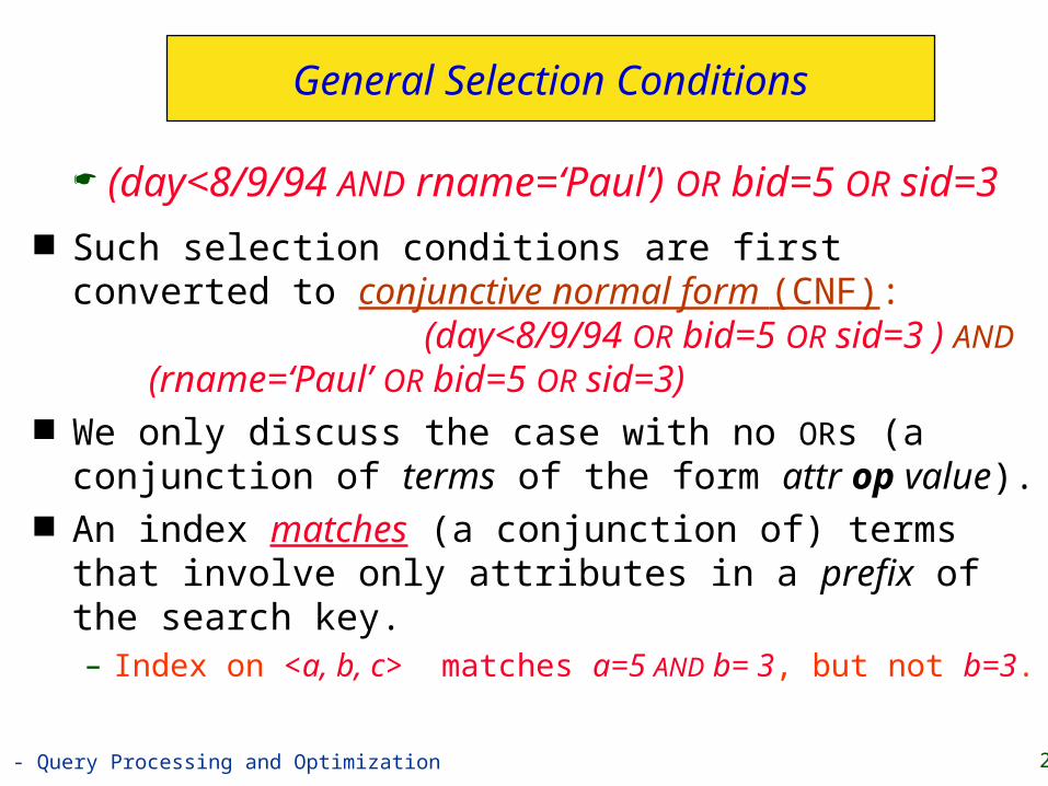
General Selection Conditions

Such selection conditions are first converted to conjunctive normal form (CNF): (day<8/9/94 OR bid=5 OR sid=3 ) AND (rname=‘Paul’ OR bid=5 OR sid=3)

We only discuss the case with no ORs (a conjunction of terms of the form attr op value).

An index matches (a conjunction of) terms that involve only attributes in a prefix of the search key.– Index on <a, b, c> matches a=5 AND b= 3, but not b=3.

(day<8/9/94 AND rname=‘Paul’) OR bid=5 OR sid=3


Two Approaches to General Selections

First approach: Find the most selective access path, retrieve tuples using it, and apply any remaining terms that don’t match the index:– Most selective access path: An index or file scan that we

estimate will require the fewest page I/Os.– Terms that match this index reduce the number of tuples

retrieved; other terms are used to discard some retrieved tuples, but do not affect number of tuples/pages fetched.

– Consider day<8/9/94 AND bid=5 AND sid=3. A B+ tree index on day can be used; then, bid=5 and sid=3 must be checked for each retrieved tuple. Similarly, a hash index on <bid, sid> could be used; day<8/9/94 must then be checked.


Intersection of Rids

Second approach (if we have 2 or more matching indexes that use Alternatives (2) or (3) for data entries):– Get sets of rids of data records using each matching index.– Then intersect these sets of rids (we’ll discuss intersection

soon!)– Retrieve the records and apply any remaining terms.– Consider day<8/9/94 AND bid=5 AND sid=3. If we have a

B+ tree index on day and an index on sid, both using Alternative (2), we can retrieve rids of records satisfying day<8/9/94 using the first, rids of recs satisfying sid=3 using the second, intersect, retrieve records and check bid=5.


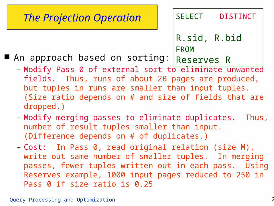
The Projection Operation

An approach based on sorting:– Modify Pass 0 of external sort to eliminate unwanted

fields. Thus, runs of about 2B pages are produced, but tuples in runs are smaller than input tuples. (Size ratio depends on # and size of fields that are dropped.)

– Modify merging passes to eliminate duplicates. Thus, number of result tuples smaller than input. (Difference depends on # of duplicates.)

– Cost: In Pass 0, read original relation (size M), write out same number of smaller tuples. In merging passes, fewer tuples written out in each pass. Using Reserves example, 1000 input pages reduced to 250 in Pass 0 if size ratio is 0.25

SELECT DISTINCT R.sid, R.bidFROM Reserves R


Projection Based on Hashing

Partitioning phase: Read R using one input buffer. For each tuple, discard unwanted fields, apply hash function h1 to choose one of B-1 output buffers.– Result is B-1 partitions (of tuples with no unwanted fields).

2 tuples from different partitions guaranteed to be distinct. Duplicate elimination phase: For each partition, read

it and build an in-memory hash table, using hash fn h2 (<> h1) on all fields, while discarding duplicates.– If partition does not fit in memory, can apply hash-based

projection algorithm recursively to this partition. Cost: For partitioning, read R, write out each tuple,

but with fewer fields. This is read in next phase.


Discussion of Projection

Sort-based approach is the standard; better handling of skew and result is sorted.

If an index on the relation contains all wanted attributes in its search key, can do index-only scan.– Apply projection techniques to data entries (much

smaller!) If an ordered (i.e., tree) index contains all wanted

attributes as prefix of search key, can do even better:– Retrieve data entries in order (index-only scan), discard

unwanted fields, compare adjacent tuples to check for duplicates.


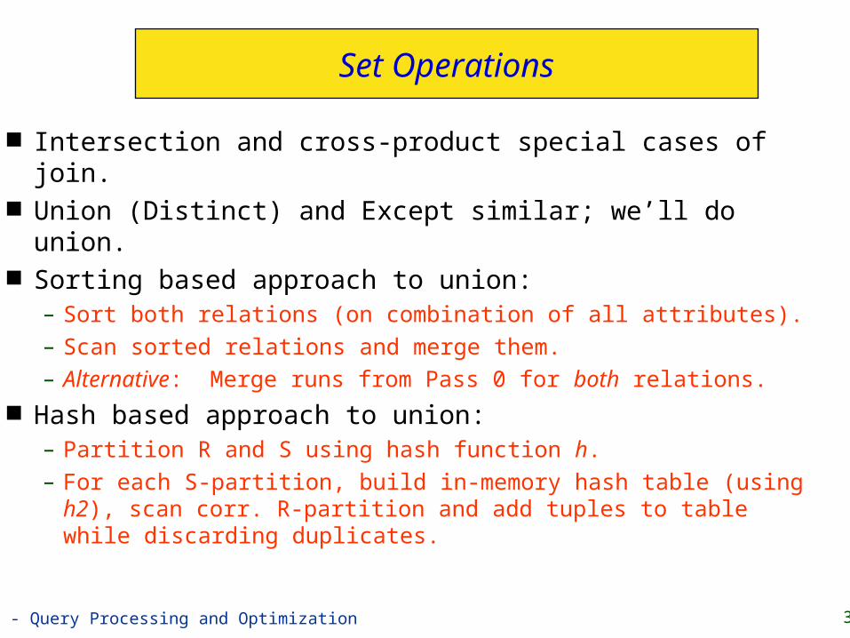
Set Operations

Intersection and cross-product special cases of join. Union (Distinct) and Except similar; we’ll do union. Sorting based approach to union:

– Sort both relations (on combination of all attributes).– Scan sorted relations and merge them.– Alternative: Merge runs from Pass 0 for both relations.

Hash based approach to union:– Partition R and S using hash function h.– For each S-partition, build in-memory hash table (using

h2), scan corr. R-partition and add tuples to table while discarding duplicates.


Aggregate Operations (AVG, MIN, etc.)

Without grouping:– In general, requires scanning the relation.– Given index whose search key includes all attributes in

the SELECT or WHERE clauses, can do index-only scan. With grouping:

– Sort on group-by attributes, then scan relation and compute aggregate for each group. (Can improve upon this by combining sorting and aggregate computation.)

– Given tree index whose search key includes all attributes in SELECT, WHERE and GROUP BY clauses, can do index-only scan; if group-by attributes form prefix of search key, can retrieve data entries/tuples in group-by order.


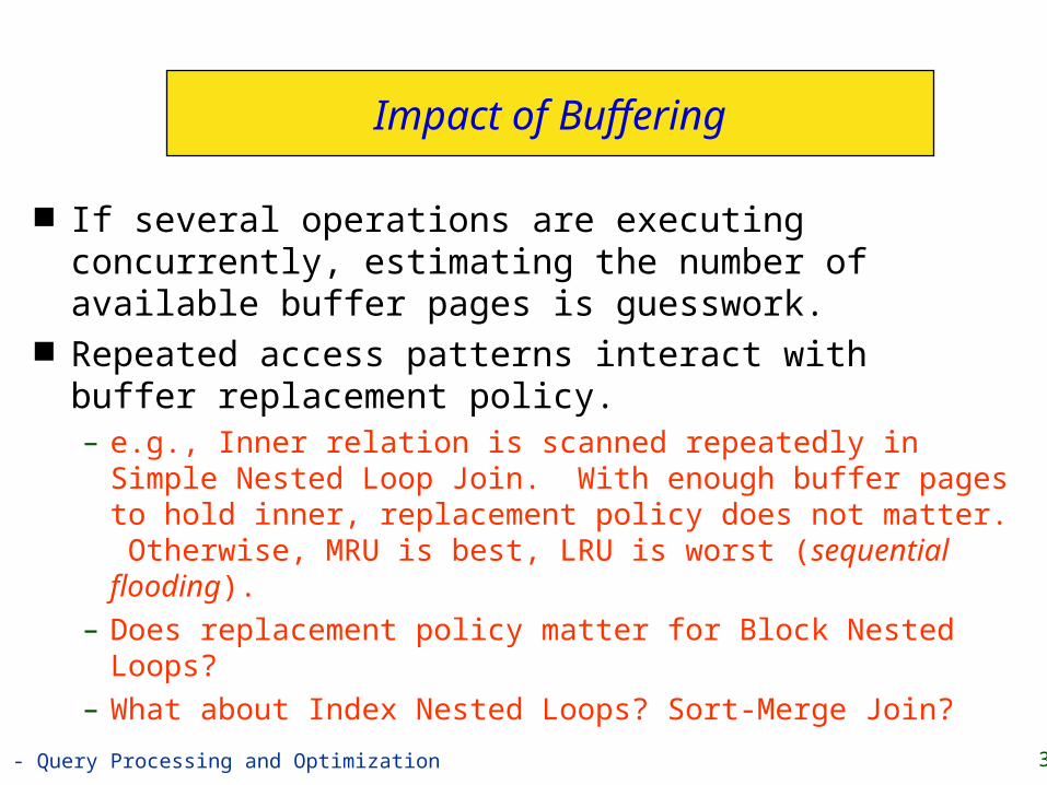
Impact of Buffering

If several operations are executing concurrently, estimating the number of available buffer pages is guesswork.

Repeated access patterns interact with buffer replacement policy.– e.g., Inner relation is scanned repeatedly in Simple

Nested Loop Join. With enough buffer pages to hold inner, replacement policy does not matter. Otherwise, MRU is best, LRU is worst (sequential flooding).

– Does replacement policy matter for Block Nested Loops?

– What about Index Nested Loops? Sort-Merge Join?


Summary for Relational Operators Implementation

A virtue of relational DBMSs: queries are composed of a few basic operators; the implementation of these operators can be carefully tuned (and it is important to do this!).

Many alternative implementation techniques for each operator; no universally superior technique for most operators.

Must consider available alternatives for each operation in a query and choose best one based on system statistics, etc. This is part of the broader task of optimizing a query composed of several ops.


Overview of Query Optimization

Plan: Tree of R.A. ops, with choice of alg for each op.– Each operator typically implemented using a `pull’

interface: when an operator is `pulled’ for the next output tuples, it `pulls’ on its inputs and computes them.

Two main issues:– For a given query, what plans are considered?

Algorithm to search plan space for cheapest (estimated) plan.

– How is the cost of a plan estimated? Ideally: Want to find best plan. Practically: Avoid

worst plans! We will study the System R approach.


Highlights of System R Optimizer

Impact:– Most widely usedcurrently; works well for < 10 joins.

Cost estimation: Approximate art at best.– Statistics, maintained in system catalogs, used to

estimate cost of operations and result sizes.– Considers combination of CPU and I/O costs.

Plan Space: Too large, must be pruned.– Only the space of left-deep plans is considered.

Left-deep plans allow output of each operator to be pipelined into the next operator without storing it in a temporary relation.

– Cartesian products avoided.


Schema for Examples

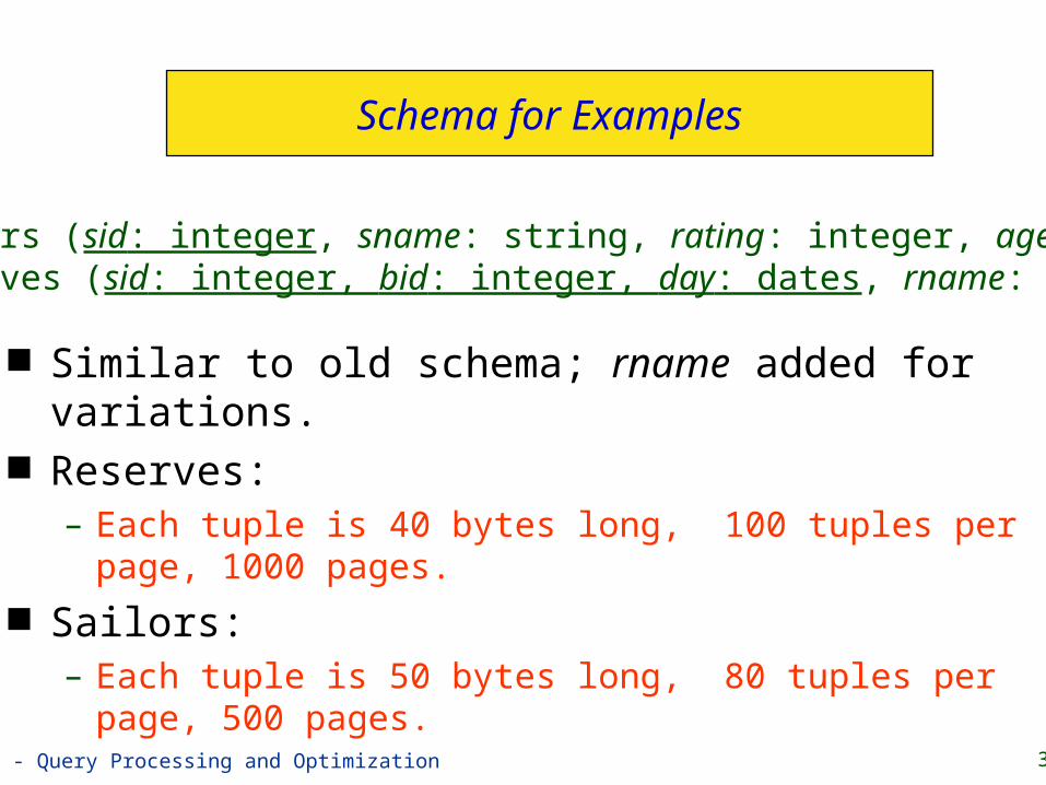
Similar to old schema; rname added for variations.

Reserves:– Each tuple is 40 bytes long, 100 tuples per page,

1000 pages. Sailors:

– Each tuple is 50 bytes long, 80 tuples per page, 500 pages.

Sailors (sid: integer, sname: string, rating: integer, age: real)Reserves (sid: integer, bid: integer, day: dates, rname: string)


Motivating Example

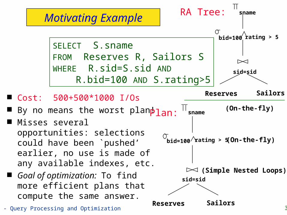
Cost: 500+500*1000 I/Os By no means the worst plan! Misses several opportunities:

selections could have been `pushed’ earlier, no use is made of any available indexes, etc.

Goal of optimization: To find more efficient plans that compute the same answer.

SELECT S.snameFROM Reserves R, Sailors SWHERE R.sid=S.sid AND R.bid=100 AND S.rating>5

Reserves Sailors

sid=sid

bid=100 rating > 5

sname

Reserves Sailors

sid=sid

bid=100 rating > 5

sname

(Simple Nested Loops)

(On-the-fly)

(On-the-fly)

RA Tree:

Plan:


Alternative Plans 1 (No Indexes)

Main difference: push selects. With 5 buffers, cost of plan:

– Scan Reserves (1000) + write temp T1 (10 pages, if we have 100 boats, uniform distribution).

– Scan Sailors (500) + write temp T2 (250 pages, if we have 10 ratings).– Sort T1 (2*2*10), sort T2 (2*3*250), merge (10+250)– Total: 3560 page I/Os.

If we used BNL join, join cost = 10+4*250, total cost = 2770. If we `push’ projections, T1 has only sid, T2 only sid and

sname:– T1 fits in 3 pages, cost of BNL drops to under 250 pages, total < 2000.

Reserves Sailors

sid=sid

bid=100

sname(On-the-fly)

rating > 5(Scan;write to temp T1)

(Scan;write totemp T2)

(Sort-Merge Join)


Alternative Plans 2With Indexes

With clustered index on bid of Reserves, we get 100,000/100 = 1000 tuples on 1000/100 = 10 pages.

INL with pipelining (outer is not materialized).

Decision not to push rating>5 before the join is based on availability of sid index on Sailors. Cost: Selection of Reserves tuples (10 I/Os); for each, must get matching Sailors tuple (1000*1.2); total 1210 I/Os.

Join column sid is a key for Sailors.–At most one matching tuple, unclustered index on sid OK.

–Projecting out unnecessary fields from outer doesn’t help.

Reserves

Sailors

sid=sid

bid=100

sname(On-the-fly)

rating > 5

(Use hashindex; donot writeresult to temp)

(Index Nested Loops,with pipelining )

(On-the-fly)


Query Blocks: Units of Optimization

An SQL query is parsed into a collection of query blocks, and these are optimized one block at a time.

Nested blocks are usually treated as calls to a subroutine, made once per outer tuple. (This is an over-simplification, but serves for now.)

SELECT S.snameFROM Sailors SWHERE S.age IN (SELECT MAX (S2.age) FROM Sailors S2 GROUP BY S2.rating)

Nested blockOuter block For each block, the plans considered are:

– All available access methods, for each reln in FROM clause.– All left-deep join trees (i.e., all ways to join the relations one-at-a-time, with the inner reln in the FROM clause, considering all reln permutations and join methods.)


Cost Estimation

For each plan considered, must estimate cost:– Must estimate cost of each operation in plan tree.

Depends on input cardinalities. We’ve already discussed how to estimate the cost of

operations (sequential scan, index scan, joins, etc.)

– Must estimate size of result for each operation in tree! Use information about the input relations. For selections and joins, assume independence of predicates.

We’ll discuss the System R cost estimation approach.– Very inexact, but works ok in practice.– More sophisticated techniques known now.


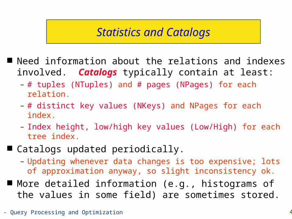
Statistics and Catalogs

Need information about the relations and indexes involved. Catalogs typically contain at least:– # tuples (NTuples) and # pages (NPages) for each

relation.– # distinct key values (NKeys) and NPages for each index.– Index height, low/high key values (Low/High) for each

tree index. Catalogs updated periodically.

– Updating whenever data changes is too expensive; lots of approximation anyway, so slight inconsistency ok.

More detailed information (e.g., histograms of the values in some field) are sometimes stored.


Size Estimation and Reduction Factors

Consider a query block: Maximum # tuples in result is the product of the

cardinalities of relations in the FROM clause. Reduction factor (RF) associated with each term

reflects the impact of the term in reducing result size. Result cardinality = Max # tuples * product of all RF’s.– Implicit assumption that terms are independent!– Term col=value has RF 1/NKeys(I), given index I on col– Term col1=col2 has RF 1/MAX(NKeys(I1), NKeys(I2))– Term col>value has RF (High(I)-value)/(High(I)-Low(I))

SELECT attribute listFROM relation listWHERE term1 AND ... AND termk


Relational Algebra Equivalences

Allow us to choose different join orders and to `push’ selections and projections ahead of joins.

Selections: (Cascade)

c cn c cnR R1 1 ... . . .

c c c cR R1 2 2 1 (Commute)

Projections: a a anR R1 1 . . . (Cascade)

Joins: R (S T) (R S) T (Associative)

(R S) (S R) (Commute)

R (S T) (T R) S Show that:


More Equivalences

A projection commutes with a selection that only uses attributes retained by the projection.

Selection between attributes of the two arguments of a cross-product converts cross-product to a join.

A selection on just attributes of R commutes with R S. (i.e., (R S) (R) S )

Similarly, if a projection follows a join R S, we can `push’ it by retaining only attributes of R (and S) that are needed for the join or are kept by the projection.


Enumeration of Alternative Plans

There are two main cases:– Single-relation plans– Multiple-relation plans

For queries over a single relation, queries consist of a combination of selects, projects, and aggregate ops:– Each available access path (file scan / index) is considered,

and the one with the least estimated cost is chosen.– The different operations are essentially carried out

together (e.g., if an index is used for a selection, projection is done for each retrieved tuple, and the resulting tuples are pipelined into the aggregate computation).


Cost Estimates for Single-Relation Plans

Index I on primary key matches selection:– Cost is Height(I)+1 for a B+ tree, about 1.2 for hash index.

Clustered index I matching one or more selects:– (NPages(I)+NPages(R)) * product of RF’s of matching selects.

Non-clustered index I matching one or more selects:– (NPages(I)+NTuples(R)) * product of RF’s of matching selects.

Sequential scan of file:– NPages(R).

Note: Typically, no duplicate elimination on projections! (Exception: Done on answers if user says DISTINCT.)


Example

If we have an index on rating:– (1/NKeys(I)) * NTuples(R) = (1/10) * 40000 tuples retrieved.– Clustered index: (1/NKeys(I)) * (NPages(I)+NPages(R)) =

(1/10) * (50+500) pages are retrieved. (This is the cost.)– Unclustered index: (1/NKeys(I)) * (NPages(I)+NTuples(R)) =

(1/10) * (50+40000) pages are retrieved. If we have an index on sid:

– Would have to retrieve all tuples/pages. With a clustered index, the cost is 50+500, with unclustered index, 50+40000.

Doing a file scan:– We retrieve all file pages (500).

SELECT S.sidFROM Sailors SWHERE S.rating=8


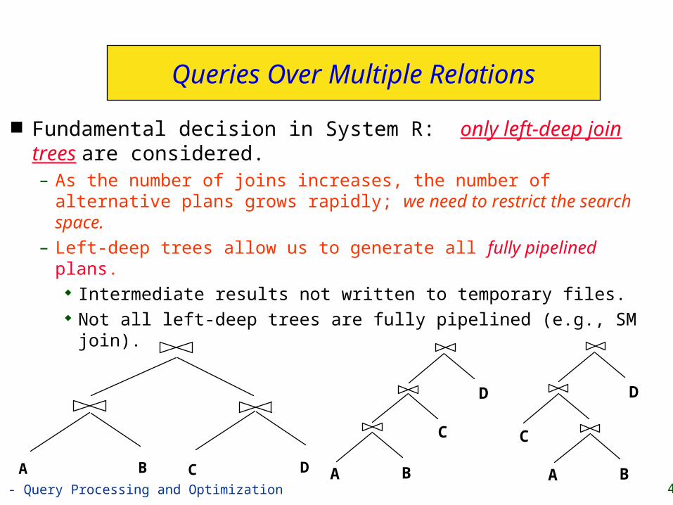
Queries Over Multiple Relations

Fundamental decision in System R: only left-deep join trees are considered.– As the number of joins increases, the number of alternative

plans grows rapidly; we need to restrict the search space.– Left-deep trees allow us to generate all fully pipelined

plans. Intermediate results not written to temporary files. Not all left-deep trees are fully pipelined (e.g., SM join).

BA

C

D

BA

C

D

C DBA


Enumeration of Left-Deep Plans

Left-deep plans differ only in the order of relations, the access method for each relation, and the join method for each join.

Enumerated using N passes (if N relations joined):– Pass 1: Find best 1-relation plan for each relation.– Pass 2: Find best way to join result of each 1-relation plan

(as outer) to another relation. (All 2-relation plans.) – Pass N: Find best way to join result of a (N-1)-relation plan

(as outer) to the N’th relation. (All N-relation plans.) For each subset of relations, retain only:

– Cheapest plan overall, plus– Cheapest plan for each interesting order of the tuples.


Enumeration of Plans (Contd.)

ORDER BY, GROUP BY, aggregates etc. handled as a final step, using either an `interestingly ordered’ plan or an addional sorting operator.

An N-1 way plan is not combined with an additional relation unless there is a join condition between them, unless all predicates in WHERE have been used up.– i.e., avoid Cartesian products if possible.

In spite of pruning plan space, this approach is still exponential in the # of tables.


Example

Pass1:– Sailors: B+ tree matches rating>5,

and is probably cheapest. However, if this selection is expected to retrieve a lot of tuples, and index is unclustered, file scan may be cheaper.

Still, B+ tree plan kept (because tuples are in rating order).

– Reserves: B+ tree on bid matches bid=500; cheapest.

Sailors: B+ tree on rating Hash on sidReserves: B+ tree on bid

Pass 2:– We consider each plan retained from Pass 1 as the outer, and consider how to join it with the (only) other relation.

e.g., Reserves as outer: Hash index can be used to get Sailors tuples that satisfy sid = outer tuple’s sid value.

Reserves Sailors

sid=sid

bid=100 rating > 5

sname


Nested Queries

Nested block is optimized independently, with the outer tuple considered as providing a selection condition.

Outer block is optimized with the cost of `calling’ nested block computation taken into account.

Implicit ordering of these blocks means that some good strategies are not considered. The non-nested version of the query is typically optimized better.

SELECT S.snameFROM Sailors SWHERE EXISTS (SELECT * FROM Reserves R WHERE R.bid=103 AND R.sid=S.sid)

Nested block to optimize: SELECT * FROM Reserves R WHERE R.bid=103 AND S.sid= outer valueEquivalent non-nested query:

SELECT S.snameFROM Sailors S, Reserves RWHERE S.sid=R.sid AND R.bid=103


Summary for Query Optimization

Query optimization is an important task in a relational DBMS.

Must understand optimization in order to understand the performance impact of a given database design (relations, indexes) on a workload (set of queries).

Two parts to optimizing a query:– Consider a set of alternative plans.

Must prune search space; typically, left-deep plans only.

– Must estimate cost of each plan that is considered. Must estimate size of result and cost for each plan node. Key issues: Statistics, indexes, operator implementations.


Summary (Contd.)

Single-relation queries:– All access paths considered, cheapest is chosen.– Issues: Selections that match index, whether index key has

all needed fields and/or provides tuples in a desired order. Multiple-relation queries:

– All single-relation plans are first enumerated. Selections/projections considered as early as possible.

– Next, for each 1-relation plan, all ways of joining another relation (as inner) are considered.

– Next, for each 2-relation plan that is `retained’, all ways of joining another relation (as inner) are considered, etc.

– At each level, for each subset of relations, only best plan for each interesting order of tuples is `retained’.

Documents

YV - Query Processing and Optimization 369 Κεφάλαιο 9 Επεξεργασία και Βελτιστοποίηση Ερωτήσεων σε Σχεσιακές Βάσεις Δεδομένων